Projective Symmetry and Coherence Regimes in the Eady Model of Baroclinic Instability

Abstract

Baroclinic instability is a fundamental mechanism of midlatitude atmospheric variability, and the Eady model remains one of its most useful idealized representations. In this work, we revisit the Eady configuration from the viewpoint of solution-space geometry rather than the classical normal-mode/growth-rate analysis. Starting from the reduced Eady vertical-structure equation, we show that the ratio of two independent solutions satisfies a Schwarzian-type relation that is invariant under homographic transformations, which naturally leads to an SL(2R) projective symmetry of the solution family. On this basis, we introduce a complex amplitude representation and reformulate coherence in terms of phase–amplitude synchronization constrained by projective invariants. Using Riccati-type constructions along geodesic parametrizations, the reduced dynamics are connected to a Stoler-type transform. Numerical exploration of the reduced model shows a systematic dependence on the control parameter $\omega$: small $\omega$ is associated with simple oscillatory or burst-like behavior, intermediate $\omega$ with period-doubling-like behavior, and large $\omega$ with strongly modulated dynamics and more intricate reconstructed attractors. These results should be interpreted as properties of the reduced symmetry-based model, and they suggest that projective invariants may provide a useful framework for classifying organization regimes in Eady-type disturbances, complementary to classical growth-rate analyses.

1. Introduction

Baroclinic instability is a fundamental mechanism of midlatitude atmospheric variability, and the Eady model remains one of its most important idealized formulations because it isolates the combined roles of rotation, stratification, and vertical shear in a mathematically transparent setting. For this reason, the Eady problem has long served as a benchmark for understanding the growth of synoptic-scale disturbances and for interpreting the preferred scales and structures of developing baroclinic waves [1,2].

In the classical literature, the Eady model is usually analyzed in terms of normal modes, growth rates, phase speeds, and the coupling of boundary-trapped disturbances. These aspects are well established, and they explain why the model has retained its value as both a pedagogical and a theoretical reference. In the present work, however, our aim is not to revisit those classical results in detail, but to consider a different question: whether the reduced Eady vertical problem also contains a useful geometric structure at the level of the solution space itself.

This is the point at which the use of SL(2R) becomes natural. Once the reduced Eady equation is written as a second-order linear ordinary differential equation, the ratio of two linearly independent solutions is defined only up to homographic (Möbius) transformations. The relevant invariance class is therefore projective, and its natural symmetry group is SL(2R). In this sense, SL(2R) is not introduced here as an external analogy borrowed from other areas of physics or mathematics, but as a structure already implied by the solution family of the reduced Eady equation. This observation motivates our use of projective invariants and Riccati-type constructions as tools for describing disturbance organization.

The purpose of this paper is therefore narrower than a full physical reformulation of baroclinic instability. We use the Eady setting as a mathematically controlled prototype in which the projective structure of the reduced equation can be examined explicitly, and we explore whether this structure supports a coherence-based classification of model dynamics. The results should accordingly be read as a proof-of-concept reduced-order framework for Eady-type disturbances, rather than as a direct predictive model of real cyclone evolution.

In addition to the classical Eady formulation, baroclinic instability has also been studied through several related mathematical frameworks, including Charney-type quasi-geostrophic models with meridional potential-vorticity gradients [3,4], Phillips-type layered models [5], Green-type extensions of baroclinic stability, and more physically complete frontogenesis, life-cycle, or moist-baroclinic formulations [5,6,7,8,9,10]. These approaches are typically interpreted through modal growth rates, phase speeds, energetics, or wave–mean-flow interaction. By contrast, the present study does not seek a more complete physical closure than those models. Its purpose is different: to examine whether the reduced Eady vertical equation possesses an intrinsic projective structure that can be used to classify disturbance organization in terms of phase–amplitude coherence. In this sense, the framework proposed here should be regarded as a complementary reduced-order geometric description, rather than as a substitute for standard quasi-geostrophic or fully nonlinear atmospheric models.

2. Mathematical Model

Let us consider the Eady model in the form

$${\psi }^{″}+\left[{\displaystyle \frac{N^2{k}^2}{f_0^2\left(\omega -kU\right)}}-k^2\right]\psi =0$$

(1)

where $\psi$ is a geostrophic current function of the perturbation, $U$ is the median flow, $\omega$ is the perturbation frequency, $k$ is a wave number, $f_0$ is the Coriolis factor, and $N$ is the Brunt–Väisälä frequency [11,12,13].

In the present reduced formulation, the disturbance field is represented through a complex amplitude whose modulus and phase provide a compact description of the organization of the solution. The term “structural units” is used here only in the reduced-model sense to denote interacting components of this complex representation, and should not be interpreted as discrete physical atmospheric entities. Our objective is to characterize how this reduced representation changes under the symmetries of the governing equation and how those changes are reflected in the coherence properties of the model dynamics.

In the following, we will focus on the case for which $k_0^2=\mathrm{c}\mathrm{o}\mathrm{n}\mathrm{s}\mathrm{t}.$, $k_0^2>0$, and

$$k_0^2\equiv {\displaystyle \frac{N^2{k}^2}{f_0^2\left(\omega -kU\right)}}-k^2$$

(2)

Then, Equation (1) takes the form

$${\displaystyle \frac{d^2\Psi }{d{x}^2}}+k_0^2\Psi =0$$

(3)

The solution of Equation (3) can be written as

$$\Psi \left(x\right)=h{e}^{i\left(k_{0}x+\theta \right)}+\acute{h}{e}^{-i\left(k_{0}x+\theta \right)}$$

(4)

where $h$ is the complex amplitude, $\acute{h}$ is the complex conjugate of $h$, and $\theta$ is a phase. Consequently, $h$, $\acute{h}$ and $\theta$ designate each atmospheric structural unit that possesses the identical fundamental attribute $k_0$.

Equation (3) exhibits a “hidden” symmetry through a homographic group. The ratio $\epsilon$ of two independent linear solutions of Equation (3) constitutes a solution of Schwartz’s differential equation [14]:

$$\left\{\epsilon ,x\right\}={\displaystyle \frac{d}{dx}}\left({\displaystyle \frac{\ddot{\epsilon }}{\dot{\epsilon }}}\right)-{\displaystyle \frac{1}{2}}{\left({\displaystyle \frac{\ddot{\epsilon }}{\dot{\epsilon }}}\right)}^2=2k_0^2$$

(5)

$$\dot{\epsilon }={\displaystyle \frac{d\epsilon }{dx}},\ddot{\epsilon }={\displaystyle \frac{d^2\epsilon }{d{x}^2}}$$

(6)

The left side of Equation (5) is invariant with respect to the homographic transformations:

$$\epsilon \leftrightarrow {\epsilon }^{\prime }={\displaystyle \frac{a\epsilon +b}{c\epsilon +d}}$$

(7)

with $a$, $b$, $c$ and $d$ being real parameters. Equation (7), encompassing all potential values of these parameters, delineates the SL(2R) group [15].

At this stage, it is useful to stress why the SL(2R) structure is relevant in the present context. The reduced Eady vertical equation is a second-order linear equation, and the ratio of two independent solutions is therefore only defined up to homographic transformations. The emergence of SL(2R) is thus not imposed from outside the problem; it follows from the intrinsic projective freedom of the solution family. Our use of this symmetry is intended to organize the admissible reduced dynamics and to examine whether the quantities preserved under these transformations can serve as descriptors of coherence in the model.

We will now reexamine Equation (7), which represents the homographic action of the generic matrix:

$$\widehat{M}=\left(\begin{array}{cc}\alpha & \beta \\ \gamma & \delta \end{array}\right)$$

(8)

In this regard, let us concentrate on the subsequent points: a relationship must be established among the set of matrices $\widehat{M}$ and the ensemble of values corresponding to $\epsilon$, for which ${\epsilon }^{\prime }$ remains constant.

From a geometric perspective, this involves determining the collection of points $\left(\alpha ,\beta ,\gamma ,\delta \right)$, univocally corresponding to the values of the parameter $\epsilon$. By using Equation (7), along with the methods from [16,17,18] (i.e., Riccati-type gauge), we obtain

$$d\epsilon +{\omega }_1{\epsilon }^2+{\omega }_2\epsilon +{\omega }_3=0$$

(9)

where the following notations are used [17,19]:

$$\begin{array}{c}{\omega }_1={\displaystyle \frac{\gamma d\alpha -\alpha d\gamma }{\alpha \delta -\beta \gamma }}, {\omega }_2={\displaystyle \frac{\delta d\alpha -\alpha d\delta +\gamma d\beta -\beta d\gamma }{\alpha \delta -\beta \gamma }},\\ {\omega }_3={\displaystyle \frac{\delta d\beta -\beta d\delta }{\alpha \delta -\beta \gamma }}\end{array}$$

(10)

It is evident that the metric

$$d{s}^2={\displaystyle \frac{{\left(\alpha d\delta +\delta d\alpha -\beta d\gamma -\gamma d\beta \right)}^2}{4{\left(\alpha \delta -\beta \gamma \right)}^2}}-{\displaystyle \frac{d\alpha d\delta -d\beta d\gamma }{\alpha \delta -\beta \gamma }}$$

(11)

is in a direct relation with the discriminant of the quadratic polynomial from Equation (9):

$$d{s}^2={\displaystyle \frac{1}{4}}\left({{\omega }_2}^2-4{\omega }_1{\omega }_2\right)$$

(12)

It is imperative to highlight that, for a particular case of 1-forms ${\omega }_1,{\omega }_2,{\omega }_3$ [17,19], the metric (12) also admits the SL(2R) invariance.

The three differential forms from Equation (10) can provide a coframe [17,19] in any point of the absolute space. This enables the transformation of the geometric properties of absolute space into algebraic attributes linked to differential Equation (9).

In this case, the 1-forms ${\omega }_1,{\omega }_2,{\omega }_3$ are differentiated exactly in the same parameter $\tau$ of the geodesic. Along these geodesics, Equation (9) can be transformed into a Riccati-type differential equation:

$${\displaystyle \frac{d\epsilon }{d\tau }}=P\left(\epsilon \right), P\left(\epsilon \right)=c_1{\epsilon }^2+2c_2\epsilon +c_3$$

(13)

The constants $c_1$, $c_2$, $c_3$ characterize a specific geodesic of the family. In this case, by employing the method from [19,20], Equation (13) highlights the dynamics correlated by a Stoler transform [21]:

$$z=-{\displaystyle \frac{c_2}{c_1}}+{\displaystyle \frac{\omega }{c_1}}\left[{\displaystyle \frac{2r\sin \left[2\omega \left(\tau -{\tau }_0\right)\right]}{1+r^2+2r\cos \left[2\omega \left(\tau -{\tau }_0\right)\right]}}+i{\displaystyle \frac{1-r^2}{1+r^2+2r\cos \left[2\omega \left(\tau -{\tau }_0\right)\right]}}\right]$$

(14)

where $r$ and ${\tau }_0$ are two real constants specific to the solution.

3. Results

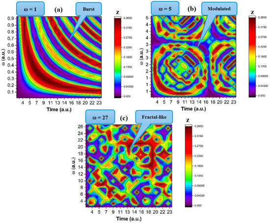
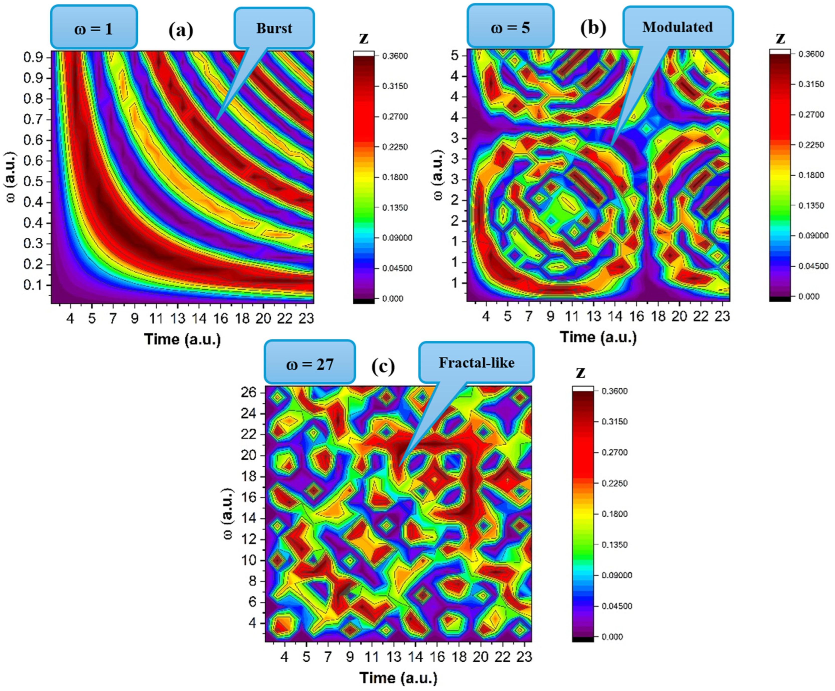
Within the present reduced formulation, the phase–amplitude synchronization modes associated with the complex representation suggest an SL(2R)-type invariance of the solution organization. The numerical behavior of the model depends systematically on the control parameter $\omega$. Figure 1a–c shows two-dimensional maps of the modulus of the complex amplitude for three representative values of $\omega$. For small $\omega$ (Figure 1a), the dynamics display burst-like or relatively simple oscillatory behavior; for intermediate $\omega$ (Figure 1b), the modulation becomes more pronounced; and for large $\omega$ (Figure 1c), the amplitude field develops a markedly more intricate texture. These changes are interpreted here as regime transitions of the reduced symmetry-based model. At the present stage, they should not be read as sharp interval boundaries in ω, but as illustrative points showing the transition toward increasingly complex organization.

Figure 1. Two-dimensional maps of the modulus of the complex amplitude for three representative values of the control parameter $\omega$: $\omega$ = 1 (a), corresponding to burst-like or relatively simple oscillatory behavior; $\omega$ = 5 (b), corresponding to a more strongly modulated regime; and $\omega$ = 27 (c), corresponding to a markedly more intricate amplitude texture. These panels illustrate representative organization regimes of the reduced model.

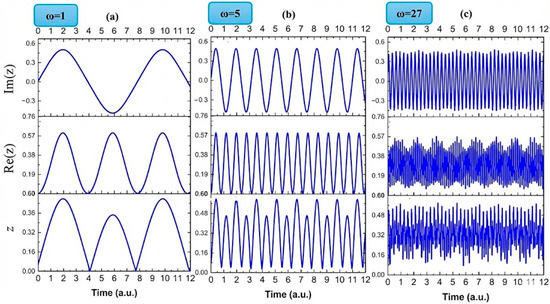
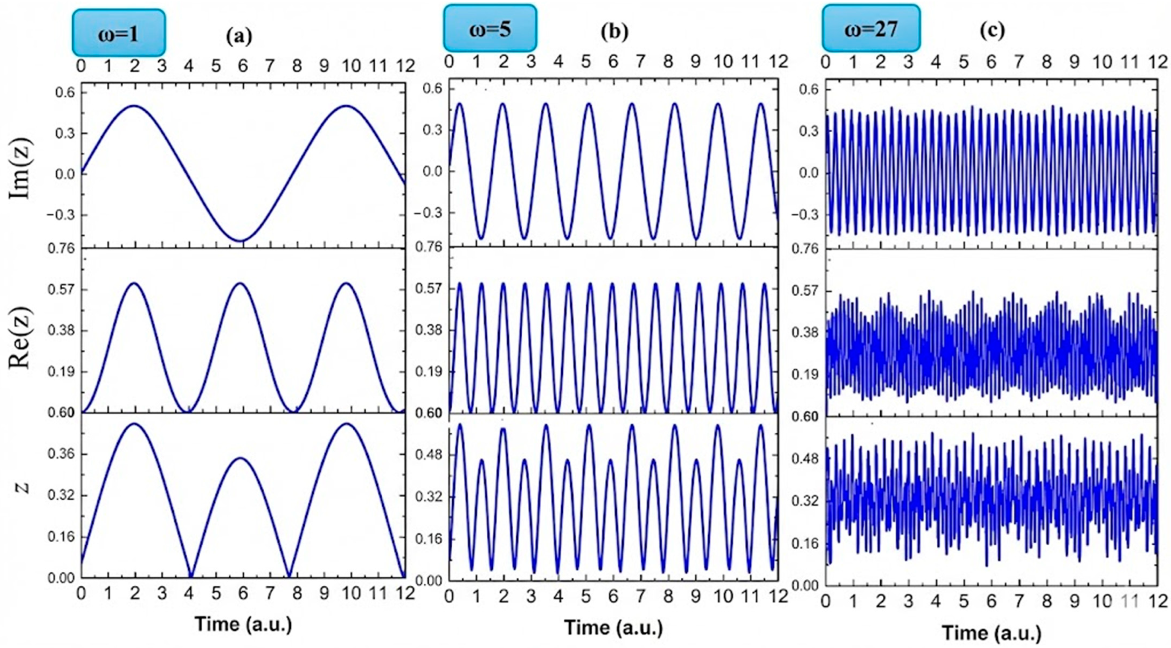
To clarify these regime changes, we extract the temporal traces of z, Im(z) and Re(z) from the corresponding two-dimensional maps. The resulting time series, shown in Figure 2a–c, indicates a progression from relatively simple oscillatory behavior at low $\omega$ (Figure 2a) to a period-doubling-like regime at intermediate $\omega$ (Figure 2b) and to strongly modulated oscillations at higher $\omega$ (Figure 2c). We therefore interpret ω as an internal control parameter of the reduced model, governing the transition from simple to increasingly complex temporal organization.

Figure 2. Time series of the oscillatory behavior for the z, Im(z) and Re(z) for various values of $\omega$, 1 (a), 5 (b), 27 (c), showing the transition from normal oscillations to modulated ones.

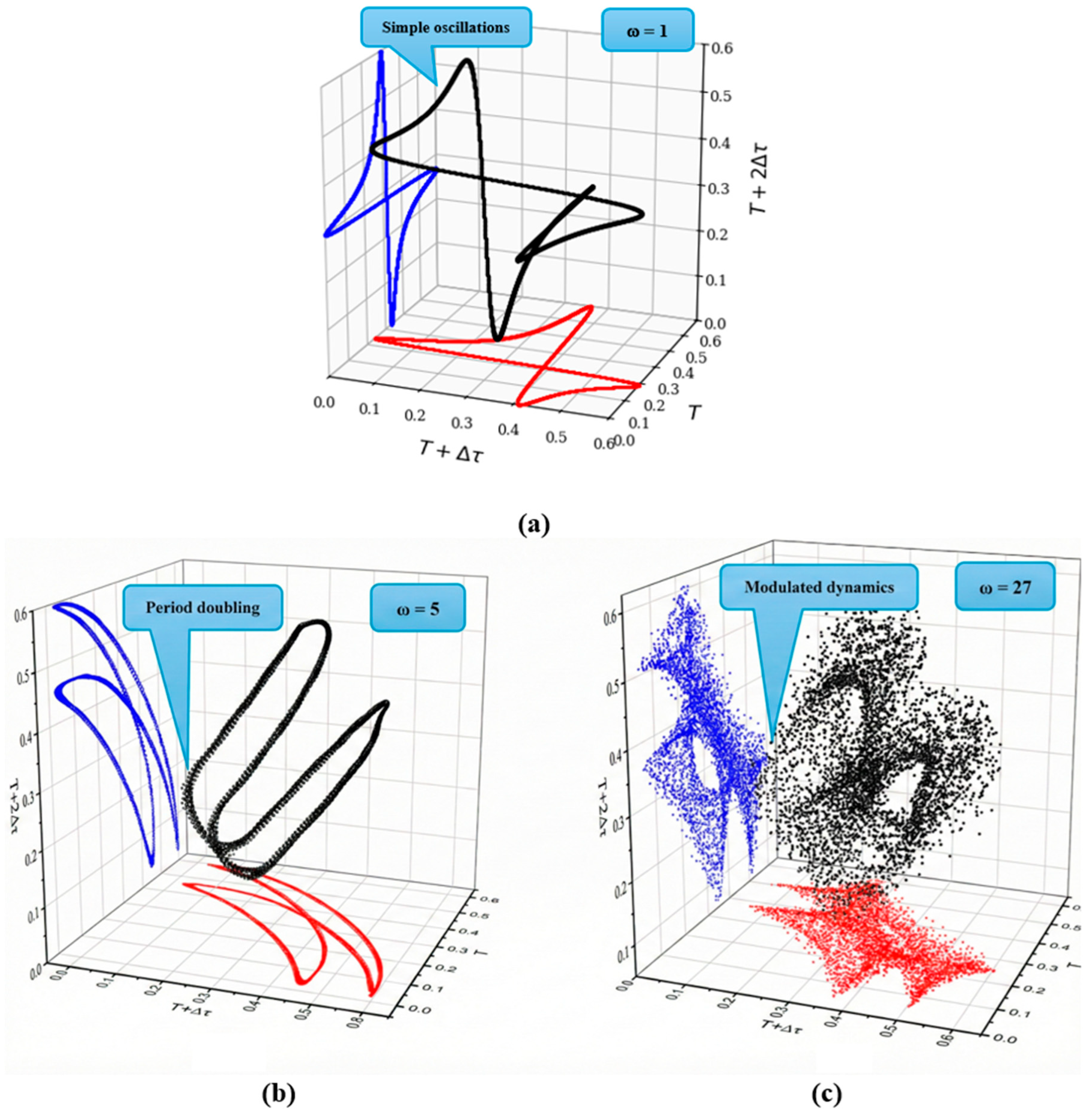
To further characterize the transition identified in the time series, we reconstruct the corresponding phase-space trajectories from the model dynamics. Figure 3 compares a representative attractor from the period-doubling-like regime with one from the strongly modulated regime. The comparison shows that increasing $\omega$ is associated not only with changes in waveform morphology, but also with a visibly more intricate phase-space organization. At the present stage, these attractors are used as qualitative signatures of regime change within the reduced model.

Figure 3. Reconstructed attractors for three representative regimes of the reduced model, $\omega$ = 1 (a), $\omega$ = 5 (b), and $\omega$ = 27 (c), showing the progression from simple oscillatory dynamics to period-doubling-like behavior and then to strongly modulated dynamics.

The parameter $\omega$ should therefore be interpreted here as a control parameter internal to the reduced symmetry-based formulation. Although it is natural to expect that $\omega$ is related to physical measures of interaction strength or scale selection, a quantitative mapping to standard Eady or quasi-geostrophic nondimensional parameters is not established in the present study. For this reason, the reported transitions are interpreted as properties of the reduced model rather than as direct predictions for observed atmospheric disturbances.

4. Discussion

The present work revisits the Eady problem from a perspective that differs from the classical normal-mode analysis. Instead of only emphasizing growth rates and phase speeds, we consider the geometry of the reduced solution space and examine the extent to which this geometry is constrained by projective invariants. In this framework, the role of the Eady model is not to provide a complete atmospheric description, but to supply a controlled setting in which the projective structure of a second-order linear problem can be analyzed explicitly.

From this viewpoint, the use of SL(2R) acquires a specific rationale. Because the ratio of two independent solutions is defined up to homographic transformations, the reduced Eady equation naturally carries a projective symmetry. The interest of this symmetry is that it allows one to ask whether organization properties of the model dynamics can be described in a way that is not visible in standard eigenvalue-based summaries. The coherence concept introduced here should therefore be understood as a property of the reduced representation, expressed in phase–amplitude variables and constrained by projective invariance.

The numerical results indicate that the reduced model exhibits distinct regimes as $\omega$ is varied. Small $\omega$ is associated with simple or burst-like oscillatory behavior, intermediate ω with a period-doubling-like structure, and large $\omega$ with strongly modulated dynamics and more intricate phase-space trajectories. At the present stage, these patterns are best interpreted as evidence that the reduced symmetry-based formulation supports multiple organization regimes, rather than as evidence for a quantitatively established atmospheric classification.

This distinction is important for the physical interpretation of this study. In principle, the framework may suggest a complementary viewpoint to classical Eady analysis by separating instability potential from organization regime. However, such an interpretation requires further calibration. In particular, the physical meaning of $\omega$ remains to be specified more precisely, and the relationship between the reduced variables used here and standard baroclinic diagnostics must be established before stronger atmospheric conclusions can be drawn.

The main value of the present study is therefore methodological. It shows that the reduced Eady equation admits a projective symmetry interpretation that can be developed into a coherence-based description of model dynamics. A natural next step would be to connect ω to conventional baroclinic control parameters and then test whether the same organization regimes persist in more physically complete settings, such as β-plane quasi-geostrophic models or idealized baroclinic life-cycle experiments.

5. Conclusions

This work proposes a symmetry-oriented reading of the reduced Eady vertical problem in which the solution manifold, rather than only the classical normal-mode spectrum, is treated as the main object of analysis. By considering the ratio of two independent solutions, we show that the reduced equation admits a natural projective structure and that the associated invariance class is governed by SL(2R). This provides a mathematically consistent basis for describing families of admissible reduced solutions through homographic transformations and related projective invariants.

Within this framework, we introduce a complex amplitude representation in which coherence is expressed in terms of phase–amplitude organization. The numerical results show that the reduced model exhibits distinct regimes as the control parameter $\omega$ is varied, including simple oscillatory behavior, period-doubling-like behavior, and strongly modulated dynamics with more intricate reconstructed attractors. These findings demonstrate that the symmetry-based reduced formulation is rich enough to support multiple organization regimes.

At the same time, the present results should be interpreted with appropriate caution. This study does not establish a direct quantitative mapping between ω and standard atmospheric baroclinic parameters, nor does it claim direct predictive applicability to real cyclone evolution. Its main contribution is to show that the reduced Eady problem can be reformulated in a projective symmetry language that may support future reduced-order classifications of Eady-type disturbance organization. Further work should focus on parameter calibration and on testing this framework in more physically complete dynamical settings.

Compared with classical Eady-, Charney-, Green-, or Phillips-type baroclinic-instability models, which are commonly interpreted through growth rates, phase speeds, energetics, or potential-vorticity-based diagnostics, the present formulation is organized around the projective geometry of the reduced solution space and the coherence properties of a complex amplitude representation. In this respect, the model is less physically complete than moist-baroclinic, frontogenesis, or nonlinear quasi-geostrophic frameworks since it does not yet provide a direct quantitative mapping between ω and standard atmospheric control parameters. Its contribution is therefore complementary rather than substitutive: it offers a reduced-order symmetry-based framework for identifying the organization regimes of Eady-type disturbances, which may later be calibrated against more standard baroclinic diagnostics and tested in physically richer models.

References

- Eady, E.T. Long waves and cyclone waves. Tellus 1949, 1, 33–52. [Google Scholar] [CrossRef] [Scilit]
- Charney, J.G. The dynamics of long waves in a baroclinic westerly current. J. Meteorol. 1947, 4, 135–162. [Google Scholar] [CrossRef] [Scilit]
- Charney, J.G.; Eliassen, A. A numerical method for predicting the perturbations of the middle latitude westerlies. Tellus 1949, 1, 38–54. [Google Scholar] [CrossRef] [Scilit]
- Charney, J.G.; Phillips, N.A. Numerical integration of the quasi-geostrophic equations for barotropic and simple baroclinic flows. J. Atmos. Sci. 1953, 10, 71–99. [Google Scholar] [CrossRef] [Scilit]
- Phillips, N.A. Energy transformations and meridional circulations associated with simple baroclinic waves in a two-level, quasi-geostrophic model. Tellus 1954, 6, 273–286. [Google Scholar] [CrossRef] [Scilit]
- Green, J.S.A. A problem in baroclinic stability. Q. J. R. Meteorol. Soc. 1960, 86, 237–251. [Google Scholar] [CrossRef] [Scilit]
- Bretherton, F.P. Critical layer instability in baroclinic flows. Q. J. R. Meteorol. Soc. 1966, 92, 325–334. [Google Scholar] [CrossRef] [Scilit]
- Simmons, A.J.; Hoskins, B.J. The life cycles of some nonlinear baroclinic waves. J. Atmos. Sci. 1978, 35, 414–432. [Google Scholar] [CrossRef] [Scilit]
- Hoskins, B.J.; Bretherton, F.P. Atmospheric frontogenesis models: Mathematical formulation and solution. J. Atmos. Sci. 1972, 29, 11–37. [Google Scholar] [CrossRef] [Scilit]
- Emanuel, K.A.; Fantini, M.; Thorpe, A.J. Baroclinic instability in an environment of small stability to slantwise moist convection. J. Atmos. Sci. 1987, 44, 1559–1573. [Google Scholar] [CrossRef] [Scilit]
- Eliassen, A. Numerical solutions of the perturbation equation for linear flow. Tellus 1954, 6, 183–191. [Google Scholar] [CrossRef] [Scilit]
- Stone, P.H. On non-geostrophic baroclinic stability. J. Atmos. Sci. 1966, 23, 390–400. [Google Scholar] [CrossRef] [Scilit]
- Lindzen, R.S.; Farrell, B.F. A simple approximate result for the maximum growth rate of baroclinic instabilities. J. Atmos. Sci. 1980, 37, 1648–1654. [Google Scholar] [CrossRef] [Scilit]
- Orlov, Y. Schwartz′ distributions in nonlinear setting: Applications to differential equations, filtering and optimal control. Math. Probl. Eng. 2002, 8, 367–387. [Google Scholar] [CrossRef] [Scilit]
- Biswas, D.; Dutta, S. Möbius action of SL (2; R) on different homogeneous spaces. Proc. Natl. Acad. Sci. India Sect. A Phys. Sci. 2022, 92, 23–29. [Google Scholar] [CrossRef] [Scilit]
- Ghizdovat, V.; Mirila, D.C.; Nedeff, F.; Rusu, D.I.; Rusu, O.; Agop, M.; Vasincu, D. Synchronizations in Complex Systems Dynamics Through a Multifractal Procedure. Entropy 2025, 27, 647. [Google Scholar] [CrossRef] [Scilit] [PubMed]
- Ghizdovat, V.; Nazaretian, E.; Dumitras, C.G.; Agop, M.; Placinta, C.; Buzea, C.; Borsos, Z. Correlative Dynamics of Complex Systems: A Multifractal Perspective of Motion Based on SL (2R) Symmetry. Symmetry 2024, 17, 27. [Google Scholar] [CrossRef] [Scilit]
- Carinena, J.F.; Ramos, A. Integrability of the Riccati equation from a group-theoretical viewpoint. Int. J. Mod. Phys. A 1999, 14, 1935–1951. [Google Scholar] [CrossRef] [Scilit]
- Agop, M.; Irimiciuc, S.A. Multifractal Theory of Motion: From Small to Large Scales; Springer: Berlin/Heidelberg, Germany, 2024. [Google Scholar]
- Merches, I.; Agop, M. Differentiability and Fractality in Dynamics of Physical Systems; World Scientific: Singapore, 2015. [Google Scholar]
- Stoler, D. Generalized coherent states. Phys. Rev. D 1971, 4, 2309. [Google Scholar] [CrossRef] [Scilit]
Disclaimer/Publisher’s Note: The statements, opinions and data contained in all publications are solely those of the individual author(s) and contributor(s) and not of MDPI and/or the editor(s). MDPI and/or the editor(s) disclaim responsibility for any injury to people or property resulting from any ideas, methods, instructions or products referred to in the content. |
© 2026 by the authors. Licensee MDPI, Basel, Switzerland. This article is an open access article distributed under the terms and conditions of the Creative Commons Attribution (CC BY) license.