


Abstract
Accurately predicting the peak height of the F2 layer (hmF2) is crucial for radio communications, satellite navigation, and space weather studies, yet traditional empirical models often lack precision. To address this, we developed a global hmF2 prediction model using a Multilayer Perceptron (MLP) neural network, based on COSMIC radio occultation observations from 2007 to 2023. Evaluated on independent test sets from 2014 and 2019, the MLP model achieved correlation coefficients of 0.877 and 0.853 with root mean square errors of 22.3 km and 19.1 km, respectively, significantly outperforming the machine learning approaches like XGBoost and Transformer. The model also demonstrated strong generalization on an independent validation set constructed from 2014 and 2019 GIRO data, with a correlation of 0.785 and RMSE of 26.1 km, surpassing NPHM, and XGBoost. SHAP interpretability analysis identified geographic latitude, cosine of latitude, solar F10.7 index, and annual/daily harmonic terms as the most influential physical features. Error analysis showed a mean prediction error of −3.2 km and a standard deviation of 21.8 km, with stable performance during quiet periods and larger errors primarily during disturbed conditions. This study provides a reliable tool for high-accuracy hmF2 prediction and enhances the understanding of the physical mechanisms controlling its variability.
1. Introduction
The ionosphere, a region of Earth’s upper atmosphere, plays a critical role in modern technological systems by influencing the propagation of radio waves. Accurate prediction of its key parameters, such as the F2 layer peak height (hmF2), is therefore vital for ensuring the reliability of satellite navigation, high-frequency communications, and over-the-horizon radar [1,2]. Traditionally, empirical models like the International Reference Ionosphere (IRI) have provided a foundational framework for ionospheric specification. However, their performance often degrades during geomagnetically disturbed conditions and exhibits regional biases, highlighting a need for more accurate and robust forecasting tools [3,4,5].
In recent years, data-driven approaches, particularly machine learning (ML) and deep learning (DL), have revolutionized ionospheric modeling by effectively capturing complex nonlinear relationships from large datasets. Initial studies demonstrated the superiority of ML algorithms like Random Forests and Backpropagation Neural Networks over empirical models for predicting parameters such as foF2 and TEC in specific regions [6,7]. The field has since evolved towards more sophisticated hybrid architectures (e.g., CNN–BiLSTM–Attention) to better model spatiotemporal patterns [8]. Concurrently, international research has actively explored artificial neural network (ANN)-based empirical models for hmF2, with several studies demonstrating that ANNs outperform traditional empirical models in prediction accuracy [9,10]. Notably, even fundamental architectures like the MLP have proven effective and efficient for specific prediction tasks, suggesting their enduring value within a optimized framework [11,12].
Despite significant progress, key challenges persist. Predictive models frequently exhibit reduced accuracy during extreme space weather events (e.g., geomagnetic storms). Furthermore, the “black-box” nature of many complex DL models limits physical interpretability. There is also a recognized need to better harness feature engineering by deriving physically meaningful parameters to enhance model generalization. This context has renewed interest in revisiting well-structured foundational models, which, when combined with meticulous feature selection and optimization, can offer a compelling balance of performance, stability, and computational efficiency.
To address the need for a robust and globally applicable hmF2 prediction model, this study returns to a refined foundational approach. The main aim of this work is to develop a high-precision global hmF2 forecasting model based on an improved Multilayer Perceptron (MLP) architecture. By employing advanced interpretability analysis, we further seek to elucidate the core geophysical drivers controlling hmF2 variability. Our principal conclusions confirm that the proposed MLP model achieves superior accuracy compared to established empirical and ML benchmarks, while the interpretability framework successfully quantifies the influence of key features such as solar activity, geographic coordinates, and periodic cycles.
2. Data Set Construction
2.1. hmF2 Data Extraction
The radio occultation (RO) data used in this study are primarily sourced from the COSMIC-1 and COSMIC-2 missions (Taiwan Space Agency & University Corporation for Atmospheric Research, Boulder, CO, USA) The COSMIC-1 mission provided approximately 2500 electron density profiles per day, which decreased to between 1000 and 1500 profiles daily after 2011. To date, the accumulated dataset spans a complete solar cycle, comprising over 4.5 million electron density profiles in total. With its global coverage across high, middle, and low latitudes and high vertical resolution, this dataset offers an excellent foundation for investigating long-term ionospheric variations and developing high-precision models.
Data from the Global Ionosphere Radio Observatory (GIRO) network with GIRO Ionosonde (Lowell Center for Space Science and Technology, Lowell, MA, USA) serve as a crucial independent source for validation. Although providing single-station measurements, the long-term and continuous monitoring by GIRO has amassed extensive records, enabling the precise derivation of key parameters such as hmF2. Its data, covering multiple solar cycles, provide indispensable support for studies of F2 layer morphology and dynamics. Characterized by high accuracy, consistency, and reliability, the GIRO data form a solid basis for model validation and in-depth exploration of ionospheric physics.
The data were obtained from the following sources: COSMIC RO data were downloaded from the COSPDAAC data platform (https://data.cosmic.ucar.edu/gnss-ro (accessed from 1 January 2007 to 31 December 2023)). GIRO data were acquired in bulk from the Lowell GIRO Data Center (https://lgdc.uml.edu (accessed from 1 January 2007 to 31 December 2023)). The hmF2 values were extracted directly from the automatically scaled GIRO data and, after cleaning and processing, constituted the final dataset used for model training and validation.
It is important to note that the accuracy of electron density profiles retrieved from RO measurements can be affected by various factors, including solar activity and plasma irregularities. These factors can introduce sharp fluctuations in the retrieved profiles or obscure a well-defined peak, leading to deviations from the true electron density. Consequently, stringent quality control is essential prior to further analysis and application to filter out invalid electron density profiles. In this study, valid hmF2 values were obtained through the following four-step screening procedure.
(1) Define it as electron density gradient and set the range as follows:
where is the electron density gradient with the unit of el/(cm3/km); and are the lowest and highest altitudes, expressed in km; and and are the corresponding electron densities at the lowest and highest altitudes, given in el/cm3.
(2) The following definitions are used to screen the acquired COSMIC occultation observation ionospheric data:
Among them, is the original electron density, is the electron density after the original electron density is sliding averaged over 9 windows, and is the number of electron density data points in the sliding window:
(3) At the same time, the selection of the Ne profile is constrained during the processing so that the horizontal difference is within 5° to eliminate the influence of the horizontal difference on the results. The formula is set as follows:
where is the horizontal distance in km and is the electron density change at adjacent heights in el/cm3. Equation (3) is used to constrain the horizontal variation in electron density profiles, with the arctan function normalizing the ratio of horizontal distance to electron density change to the range [0, π/2]. This normalization ensures consistent weighting of horizontal variation constraints across different latitudinal and longitudinal regions, avoiding bias from dimensional differences. The physical essence is to quantify the spatial smoothness of electron density profiles, filtering out profiles with abrupt horizontal changes that may be caused by measurement noise.
(4) The peak height of the F2 layer in the COSMIC occultation ionospheric data is defined as a valid electron density profile within the following range:
Among them, is the height corresponding to the peak electron density of the F2 layer of the ionosphere, that is, the peak height.
2.2. Acquisition of Solar and Geomagnetic Activity Indices
In addition to the radio occultation and ionosonde data, the acquisition of corresponding solar and geomagnetic activity indices is essential for establishing the relationship between hmF2 and space environmental conditions from 2007 to 2023. The indices used in this study were obtained from multiple authoritative data providers, covering the entire observation period. Key parameters include the 3 h geomagnetic activity index (Kp) and its derived daily average geomagnetic activity index (Ap), the solar radio flux index (F10.7), the geomagnetic storm index (Dst), the solar wind speed (Vsw), and the sunspot number (SSN). These data were sourced from NASA’s OMNI data service (https://omniweb.gsfc.nasa.gov/form/dx1.html (accessed from 1 January 2007 to 1 January 2023)).
To ensure data quality, it is necessary to address outliers and missing values in the raw datasets. For outlier detection, the Isolation Isolation Forest algorithm in scikit-learn (v1.3.0, https://scikit-learn.org/, accessed 12 March 2026) was employed [12]. This algorithm effectively isolates anomalous data points and offers several advantages, including high computational efficiency, scalability, no assumption regarding data distribution, capability in handling high-dimensional data, and strong robustness. In this work, the contamination parameter (proportion of outliers) was set to 0.0001 to prevent an excessive replacement of data points, which could otherwise compromise the training effectiveness. For handling missing values, invalid entries (e.g., fill values of 9999) were first flagged as NaN. Subsequently, linear interpolation was applied to complete the dataset. This approach was chosen to address the limitations of simple moving-window interpolation (window sizes 5–9 tested), which fails to fill gaps adequately with insufficient valid data points in the window, thus ensuring the completeness and usability of the final dataset.
2.3. Dataset Construction
All data preprocessing was completed on a high-performance computing workstation (Dell Inc., Round Rock, TX, USA).
The features and data formats of the final compiled dataset following data quality control are presented in Table 1.
Table 1.
Main training parameters of the dataset and their corresponding meanings.
In this modeling work, we elaborately constructed a series of coupled features with clear physical meanings, aiming to enhance the model’s ability to predict and understand the key ionospheric parameter hmF2 from the in-depth dimension of spatiotemporal coupling and multi-physical field interaction. Firstly, we introduced the long-term periodic features of solar activity and characterized the quasi-periodic variation law of solar radiation intensity by performing periodic phase conversion on the year. Secondly, we calculated the Magnetic Local Time (MLT), combining geographic longitude with Local Time to more accurately describe the diurnal spatial modulation effect of the ionosphere caused by the Earth’s rotation.
It should be noted that LT, UT and Lon are not redundant input parameters, and their combination with constructed interaction terms can fully excavate the spatiotemporal coupling characteristics of the global ionosphere without severe multicollinearity, which has been verified by SHAP feature importance evaluation. To further capture the nonlinear synergetic effect between solar activity and geomagnetic activity, we constructed the product term of the solar radiation index and geomagnetic activity index. This feature can effectively characterize the response intensity of the geomagnetic field driven by intense solar events, and is particularly important for modeling ionospheric disturbances under extreme space weather conditions. Meanwhile, we considered the geometric attenuation effect in the latitudinal direction and introduced the cosine of latitude term to reflect the fundamental impact of the Earth’s spherical geometry on the distribution of ionospheric parameters.
In terms of constructing core spatiotemporal coupling features, we designed two sets of key interaction terms. LT, UT and Lon carry distinct physical information for ionospheric modeling: LT characterizes the local diurnal variation in the ionosphere driven by solar irradiation, UT reflects the global ionospheric response to space environmental disturbances at a unified time scale, and Lon represents the inherent geospatial differences in ionospheric morphology across longitudes. On this basis, the product feature of Universal Time and longitude (UT × Lon) is constructed to capture the longitudinal modulation effect caused by the Earth’s rotation, which characterizes the synchronous differences in ionospheric states across different longitudinal regions at the same absolute time on a global scale. This feature effectively helps the model analyze the phase changes and wave propagation characteristics of the ionosphere in the longitudinal direction, and thus enhances the model’s fitting ability for the global spatial distribution of hmF2. The product feature of geomagnetic disturbance index and latitude is used to represent the response gradient of geomagnetic activity disturbances in different latitudinal zones. Since the impact of geomagnetic disturbances on the ionosphere exhibits significant latitudinal dependence—especially distinct physical mechanisms in polar and equatorial regions—this feature enables the model to capture this important spatially heterogeneous response pattern.
In addition, during model training, we introduced the sine and cosine harmonic components of annual and diurnal cycles, converting cyclic time variables into continuous periodic features. This allows the model to more delicately learn the variation patterns of hmF2 with seasonal and diurnal alternations. The square term of the day of year is used to characterize the nonlinear trend component in the annual periodic variation. These physically designed feature combinations collectively enhance the model’s ability to resolve the complex spatiotemporal variation laws of the ionosphere, enabling it to more comprehensively integrate multi-dimensional information such as solar activity, geomagnetic activity, geographic coordinates, and temporal evolution, thereby improving the physical consistency and generalization performance of predictions.
We adopted a year-based dataset partitioning strategy to evaluate the model’s generalization ability across different phases of solar activity. The specific partitioning method is as follows: 2014 was selected as representative of a high-solar-activity year, corresponding to the peak phase of the 24th solar cycle, and 2019 as representative of a low-solar-activity year, corresponding to the minimum phase of the 24th solar cycle; data from the remaining 15 years (2007–2013, 2015–2018, 2020–2023) were merged into the training set. This time span fully covers the ascending phase, descending phase, and transition stages of the 24th solar cycle and includes multiple periods of moderate solar activity intensity within this cycle. This ensures that the model can learn the systematic impact of solar activity cycle variations on the ionosphere.
In the data preprocessing stage, all feature variables and the target variable hmF2 were normalized, linearly scaled to the interval [0, 1]. This standardization operation not only accelerates the convergence of model training but also avoids the unbalanced impact of different features on model weights due to dimensional differences. It is particularly noteworthy that the target value hmF2 was first subjected to logarithmic transformation to mitigate the skewness of its distribution, followed by normalization. This two-step preprocessing strategy further improves the model’s sensitivity to ionospheric height changes.
The aforementioned dataset partitioning and preprocessing methods have clear physical meanings: using years with extreme solar activity as the test set enables strict verification of the model’s extrapolation prediction ability under conditions of drastic space weather changes; and training with data from years of moderate solar activity ensures the model captures the basic variation laws of ionospheric parameters under typical solar activity levels. Normalization optimizes the training process from the perspective of numerical computation, laying a solid data foundation for subsequent machine learning modeling.
The feature design of this study is entirely based on the ionospheric physical mechanism. For the gradient feature ablation experiments on the 2014 and 2019 test sets, see Section 5.2 for details verifying the non-redundancy of the features: all included features play a complementary or core role with no substantial redundancy, and the design is scientific and reasonable.
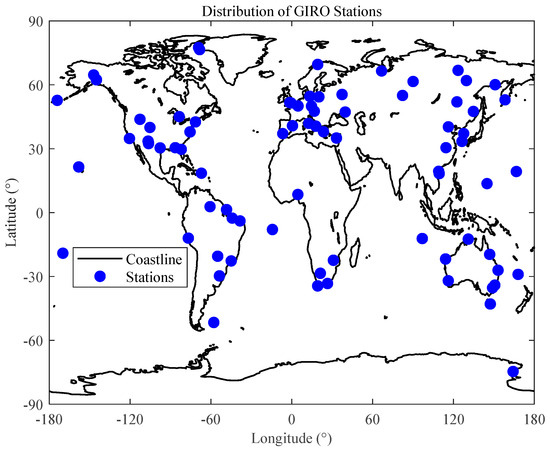
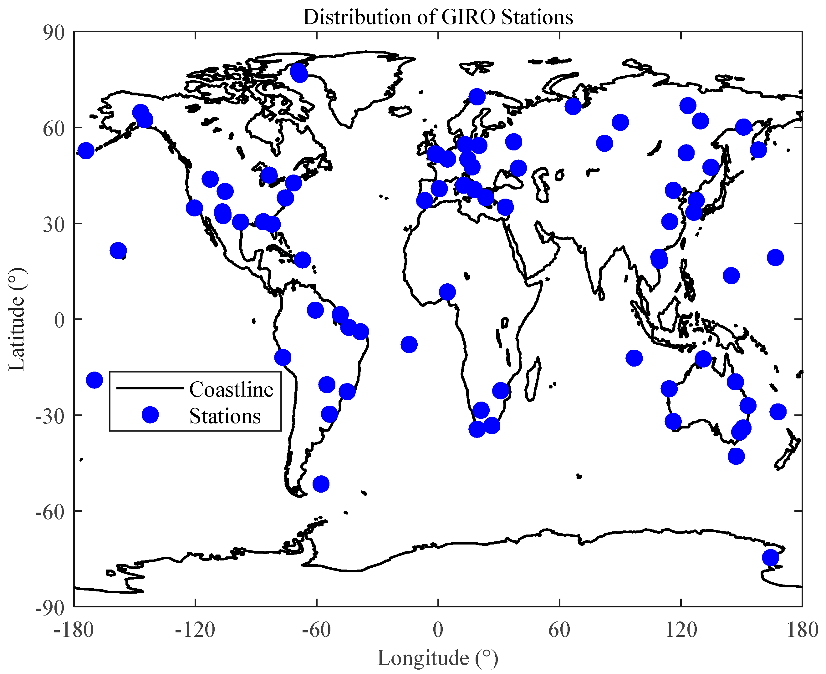
To evaluate the generalization ability of the MLP model, this study takes the observation data collected by GIRO (Global Ionospheric Radio Observatory) ionosondes at 81 stations in 2014 and 2019 as the benchmark, with the distribution of data stations shown in Figure 1. The prediction results of the model at these stations during the corresponding time periods are compared with the benchmark values to calculate the deviations. The above data form a validation dataset, containing a total of 50,000 valid samples. The detailed information of the datasets used in this study is presented in Table 2.
Figure 1.
Distribution map of GIRO stations.
Table 2.
Detailed information of datasets.
3. Modeling and Model Interpretability Analysis
Modeling Algorithm and Parameter Tuning Method Selection
All machine learning models were implemented in Python (v2023.2.1, Python Software Foundation, Wilmington, DE, USA) with relevant scientific computing libraries and MATLAB (v2022b, The MathWorks Inc., Natick, MA, USA) for data visualization and numerical simulation.
XGBoost (v1.7.6, https://xgboost.readthedocs.io/, accessed 12 March 2026), short for eXtreme Gradient Boosting, is an extended version of Gradient Boosting Decision Trees (GBDT). It optimizes the loss function by training a series of weak learners [13]. The core idea of XGBoost is to train a new weak learner in each iteration to correct the errors of the previous model. Eventually, the combination of all weak learners forms a powerful predictive model.
XGBoost uses a second-order Taylor expansion, and its loss function for the predicted value can be expressed as a second-order Taylor expansion [13]:
Among them, is the gradient of the loss function with respect to the predicted value, and is the second-order derivative of the loss function, that is, the Hessian matrix.
The attention mechanism has become an indispensable part of constructing high-performance sequence modeling and transformation models for various tasks. It enables the modeling of dependencies regardless of their distance in the input or output sequence [14,15]. Self-attention allows parallel computation, accelerating training speed while enhancing global context understanding. Transformers use self-attention to weight the importance of each token relative to others, enabling the model to dynamically focus on relevant parts of the input [16], and its mathematical implementation is shown in Equation (6).
Here, , and denote the query, key and value matrices respectively, with dk representing the dimension of the key matrix.
Multilayer Perceptrons (MLPs) are trained by means of the backpropagation algorithm to optimize network weights [17]. Studies have confirmed that as universal function approximators, MLPs can model complex nonlinear relationships [18]. Starting from the input layer, data undergo linear weighted summation layer by layer, followed by transformation through a nonlinear activation function, and finally yield the prediction result at the output layer. The computation of each layer can be expressed as
Herein, denotes the output of the l-th layer, and represent the weight matrix and bias vector of this layer, respectively, and is the nonlinear activation function. It is precisely such multi-layer nonlinear transformations that endow MLPs with powerful fitting capabilities.
Among the evaluated algorithms, the MLP achieved the highest prediction accuracy for hmF2 in 2014 and 2019, with a correlation coefficient of 0.877 and a MAE of 15.87 km, outperforming all other comparative models. Its concise architecture and superior computational efficiency further support its selection as the final model for hmF2 prediction in this study.
Considering the complexity of ionospheric data, model training efficiency, and generalization ability, the parameter settings of this study follow the following core principles, and the final determined parameter configuration is shown in Table 3.
Table 3.
MLP model training parameter configuration study.
In this study, a practical phased tuning strategy based on validation set performance monitoring was adopted instead of relying on automatic parameter search, mainly based on the following considerations and methods: The AdamW optimizer was selected, which decouples the weight decay mechanism on the basis of the Adam optimizer, enabling more efficient regularization. It is widely applied in deep learning tasks and demonstrates stable performance [19]. The cosine annealing scheduling was adopted for learning rate adjustment, a strategy that makes the learning rate gradually decrease from the initial value to the minimum value along a cosine curve, helping the model converge more accurately to the optimal solution in the later stage of training [20]. Compared with fixed learning rates or simple step decay strategies, this method generally achieves better generalization performance. To suppress overfitting of the deep neural network, a Dropout layer was introduced after each hidden layer to randomly deactivate some neurons and break feature dependencies. A Batch Normalization layer was added before the activation function of each hidden layer, which can accelerate model training, support the use of higher learning rates, and exert a certain regularization effect. The Huber loss function was chosen, as it is less sensitive to outliers than the mean squared error (MSE) [21], which can enhance the training robustness of the model on ionospheric data. To further prevent overfitting and save computational resources, an early stopping mechanism was introduced: if the validation set loss stops decreasing within a continuously set number of patience epochs, the model performance is deemed to have no room for improvement, and training is terminated immediately.
SHAP regards each feature as a participating variable in the process of model prediction. The SHAP value of a single feature reflects its contribution degree to the prediction result under different feature combinations. By eliminating the impact of feature input order through weighted averaging, the resulting SHAP values conform to the Shapley value axioms of fair allocation [22], and their mathematical expression is shown in Equation (8) [23]. The sum of the SHAP values of all features is exactly equal to the difference between the model prediction value and the baseline value, as shown in Equation (9).
- : SHAP value of the i-th feature;
- : The set of all features, totaling n;
- : The subset that does not contain feature i;
- : Model output value for subset S;
- : Model output value after including feature i;
- Weight item : Assign weights based on subset size to ensure fairness.
4. Model Evaluation
4.1. Analysis of Model Prediction Results
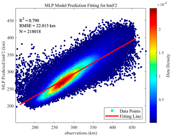
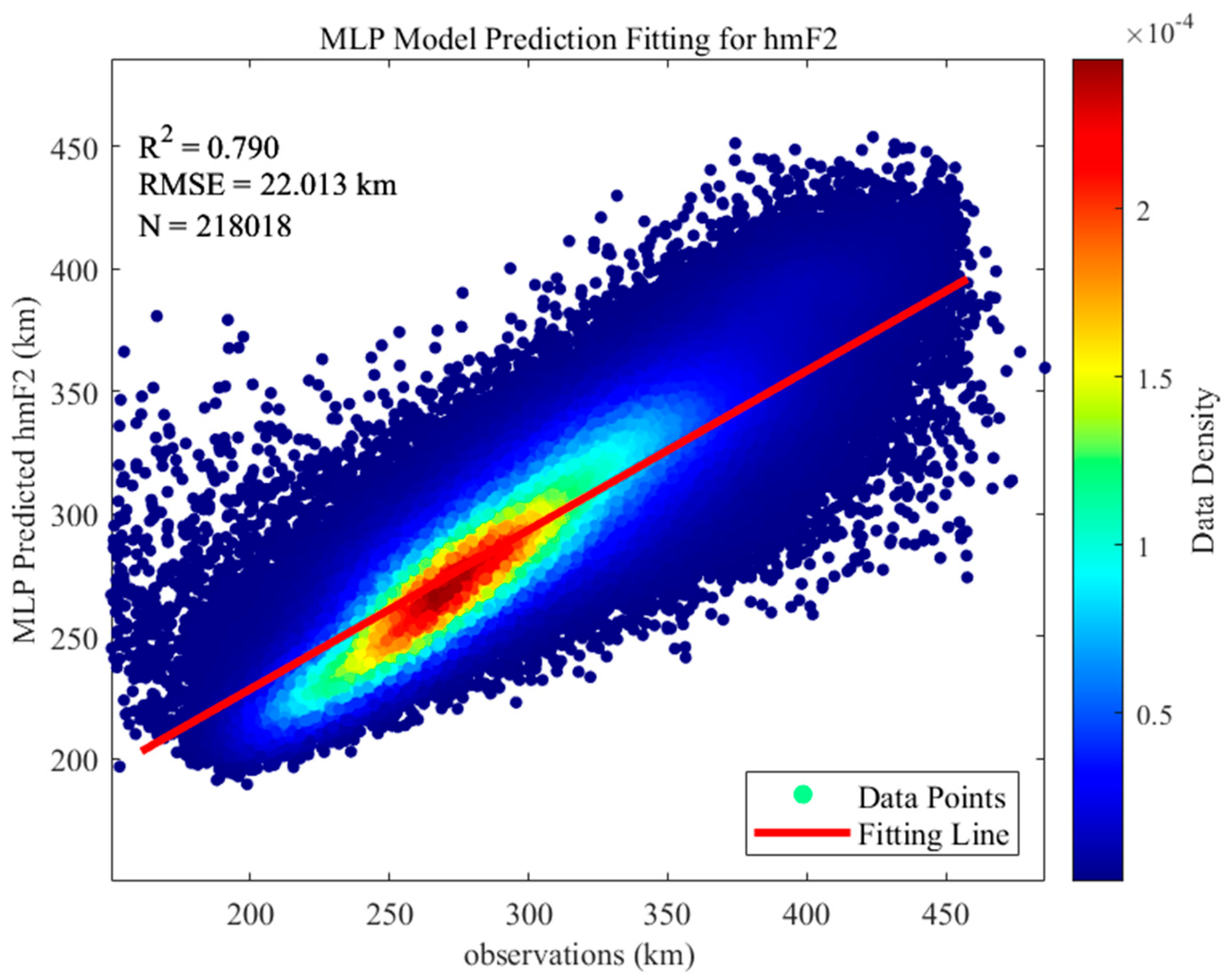
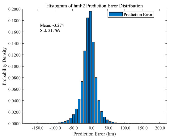
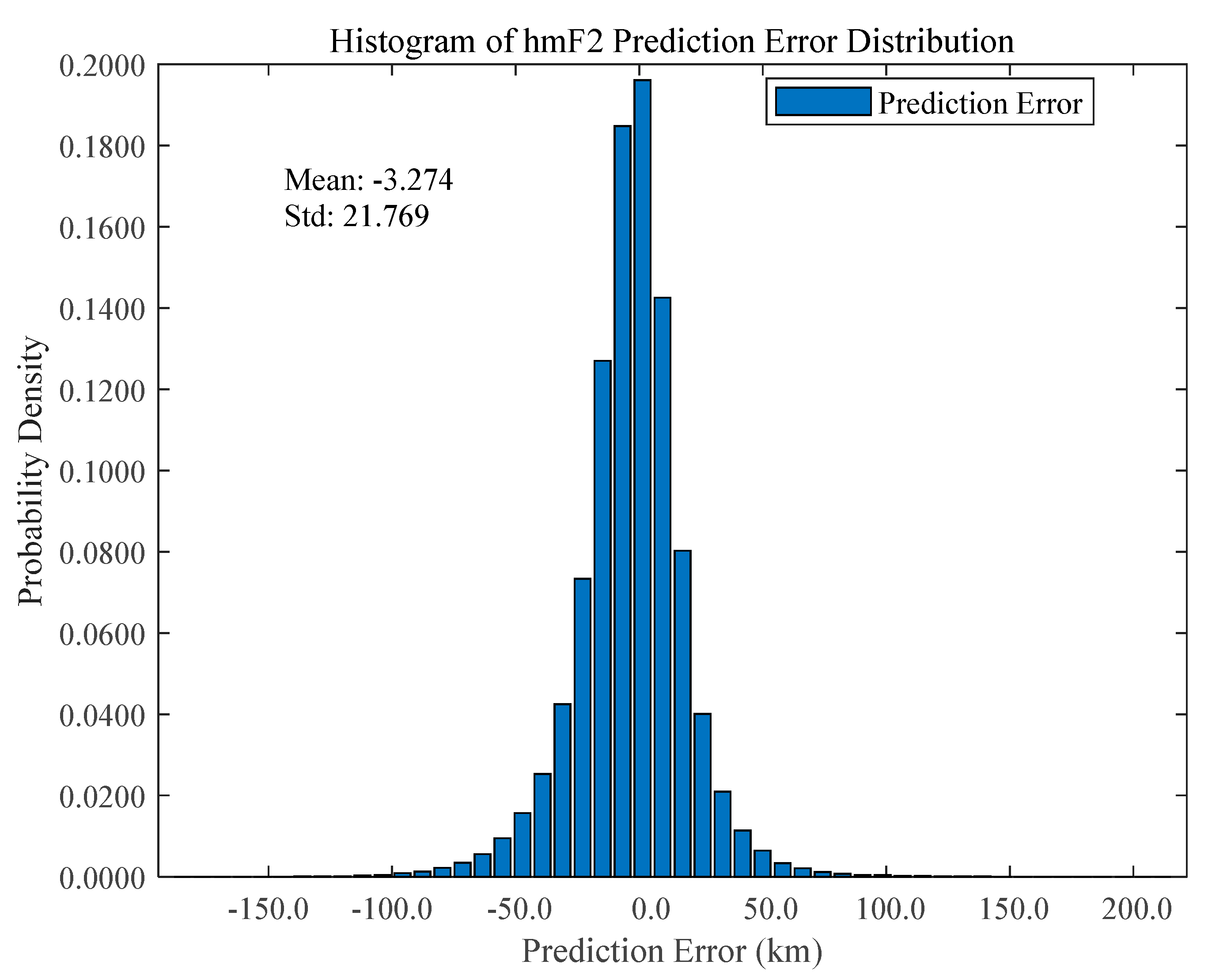
To quantitatively evaluate the prediction accuracy of the MLP model for the hmF2 parameter, this study conducted statistical analysis on the prediction errors of the COSMIC satellite test sets in 2014 and 2019. Figure 2 shows the scatter plot of MLP model predictions versus observations. The prediction errors were calculated based on Equation (10), and the histogram of the prediction error distribution was plotted as shown in Figure 3. The mean error is −3.3 km, with a standard deviation of 21.8 km. RMSE is the root mean square error between the predicted and observed values. Both are error evaluation indicators, and the RMSE takes into account both the magnitude and dispersion of errors, clarifying their physical correlation. A negative mean error indicates a slight systematic underestimation in the model’s predicted values, while a relatively large standard deviation reflects significant dispersion of the predicted values around the mean. To quantitatively characterize the actual distribution characteristics of prediction errors, this study calculated the quantile interval, skewness, and kurtosis of the error sequence. Based on the actual error distribution of the COSMIC satellite test sets in 2014 and 2019, approximately 68% of the prediction errors fall within the practical interval of [−20.7, 14.2] km. The skewness of the error distribution is −0.15, and the slightly negative skewness indicates that the error distribution is generally symmetric with a mild left-skewed tendency, which is consistent with the previous conclusion that the model occasionally underestimates hmF2 during extreme ionospheric disturbances. The raw kurtosis is 10.07 (Fisher kurtosis: 7.07), which is much larger than 3, indicating a significantly leptokurtic distribution of the error. This means that the errors of the vast majority of samples are highly concentrated near the mean, verifying the high prediction accuracy of the model under quiet ionospheric conditions. Compared with the typical dynamic range of the hmF2 parameter itself, this practical error interval demonstrates that the model can effectively capture its variation trends in most cases.
Figure 2.
MLP model prediction scatter plot of hmF2.
Figure 3.
Histogram of MLP model prediction error distribution for hmF2.
Further analysis of the error distribution histogram shows that its overall profile is basically consistent with the theoretical normal distribution curve. However, in the central region where errors are close to zero, the observed error frequency is significantly higher than the theoretical expectation, forming a prominent “peak” feature. This phenomenon indicates that the errors of the vast majority of prediction samples are extremely small, highly concentrated near zero, and the degree of concentration even exceeds the “conventional” random error range defined by the mean and standard deviation, intuitively confirming the model’s high prediction accuracy in most scenarios.
The two tails of the error distribution exhibit asymmetric deviation: negative errors extend further toward lower values, with the minimum error reaching below −60 km, which is much lower than the theoretical lower limit of the normal distribution; and positive errors are relatively sparse. This left-skewed distribution suggests that when the true hmF2 value rises sharply or sudden ionospheric disturbances occur, the model’s prediction capability is insufficient, tending to underestimate the actual height. This is also the core reason for the systematic negative deviation and the extension of the left tail of the error.
Despite the aforementioned limitations, overall, the core error of the model is within an acceptable range. Compared with the magnitude and variation range of the hmF2 parameter itself, the model’s systematic deviation is small, and it performs stably under normal ionospheric conditions. Future research can enhance the model’s prediction capability for extreme events by introducing real-time indices characterizing sudden ionospheric activities or training with a loss function more robust to outliers, thereby further compressing the left tail of the error distribution and improving overall prediction accuracy.
In summary, the “peaked and left-skewed” pattern of the error distribution reveals the core performance characteristics of the prediction model: it can achieve accurate and stable prediction for calm or normal ionospheric conditions, with strong practicality; while the prediction deviation for severe disturbance events constitutes the main source of the model’s errors.
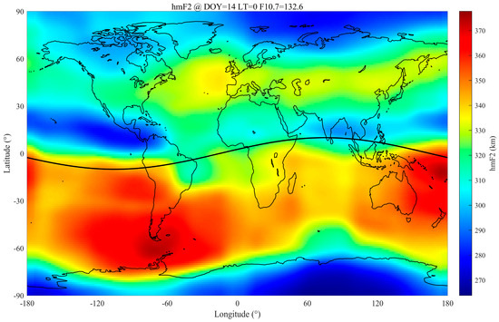
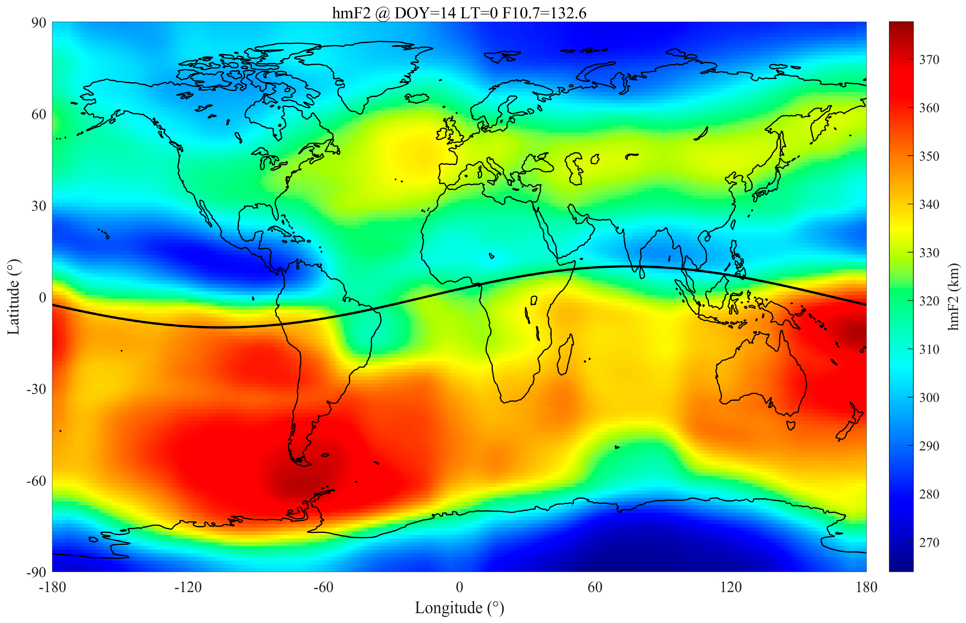
Figure 4 presents the global hmF2 distribution predicted by the model at Day of Year (DOY) = 14 and Local Time (LT) = 0. Its core characteristics can be summarized as follows: a significant hemispheric asymmetry; i.e., the overall hmF2 values in the Northern Hemisphere are lower than those in the Southern Hemisphere. In terms of latitudinal distribution, hmF2 values in the 30–60° region of the Northern Hemisphere are relatively higher than those in low and high latitudes; here is a high hmF2 region in the mid-low latitudes of the Southern Hemisphere (e.g., 0° to −70°). In addition, the Southern Hemisphere mid-low latitudes high-value region is more prominent while the magnetic equator high-value belt is a secondary feature.
Figure 4.
Global hmF2 map predicted by the MLP model.
The above distribution characteristics are a direct reflection of the coupling effects of multiple physical processes in the thermosphere–ionosphere system under specific seasonal and Local Time conditions. The core driving factors of hemispheric asymmetry are thermospheric circulation and cross-equatorial neutral winds. DOY = 14 corresponds to midsummer in the Southern Hemisphere, where intense solar ultraviolet radiation heating causes expansion and pressure increase in the thermosphere in the Southern Hemisphere, driving neutral winds to flow from the high-pressure summer hemisphere to the low-pressure winter hemisphere. The neutral winds drag ionized particles to move along inclined magnetic field lines, resulting in the uplift of hmF2 in the Southern Hemisphere (the windward side) and the depression of hmF2 in the Northern Hemisphere (the leeward side) [24]. This is consistent with the conclusions of recent observational studies based on COSMIC data, which indicate that the seasonal variation amplitude of ionospheric parameters in the Southern Hemisphere is generally larger than that in the Northern Hemisphere [25].
After midnight, the vertical electric drift in the equatorial region is usually weak or downward. In the mid-latitudes of the Northern Hemisphere winter, the field-aligned diffusion of plasma from the equator to high latitudes along magnetic field lines, combined with residual circulation effects, may serve as the dominant mechanism maintaining the relative height of hmF2 in this region. This makes hmF2 here higher than that in low latitudes dominated by rapid recombination processes and in high latitudes directly affected by energetic particle precipitation [24].
The high-value region in the mid–low latitudes of the Southern Hemisphere may be the midnight extension of the Weddell Sea Anomaly or its analogous summer anomaly [26]. A typical feature of this anomaly is the abnormal enhancement of electron density and hmF2 in specific geographical regions from dusk to the first half of the night during the Southern Hemisphere summer. This is usually closely related to the plasma transport from the dayside ionosphere to the nightside through conjugate magnetic field lines and the modulation of the neutral wind field.
The high-value belt distributed along the magnetic equator directly confirms the regulatory role of the geomagnetic field. Around midnight, there may be weak vertical electric drift in the equatorial ionosphere or residual effects of pre-reversal enhancement events, leading to slight uplift of plasma [27]. Meanwhile, the electric field associated with the equatorial electrojet and the residual impact of the equatorial fountain effect driven by it play a key regulatory role in the distribution of hmF2 in the magnetic equatorial region [28]. The high-value belt predicted by the model strictly follows the magnetic equator, demonstrating that it has successfully captured this core physical regulatory factor.
The model successfully reproduces the above global distribution structure dominated by complex physical mechanisms, indicating that it is not a mere data fitting but implicitly learns key physical processes such as thermospheric circulation, geomagnetic field geometry, equatorial electrodynamics, and interhemispheric coupling. The consistency between the prediction results and known physical laws [24] as well as recent statistical characteristics [25] verifies the physical rationality and generalization ability of the model. Particularly noteworthy is that under the specific scenario of midnight in the Northern Hemisphere winter, the model accurately predicts the overall pattern of “lower in the north and higher in the south” and the detailed feature of relative mid-latitude bulge. This performance surpasses simple symmetry or smoothness assumptions, highlighting the unique advantage of data-driven models in revealing fine spatiotemporal structures.
4.2. Comparative Analysis of Accuracy Between MLP and Other Prediction Models
The Neustrelitz Peak Height Model (NPHM) is a nonlinear empirical model for the peak height of the global ionospheric F2 layer. Based on 13 polynomial coefficients and several empirical fixed parameters, this model is constructed by fitting GNSS radio occultation data from CHAMP, GRACE, COSMIC and global ionosonde data via the nonlinear least squares method [29].
The core formula for calculating hmF2 using NPHM is as follows:
- : diurnal variation;
- : annual and semiannual variations;
- : geomagnetic latitude variation;
- : solar activity dependence.
Different from empirical models, this study employs a Transformer model based on the self-attention mechanism to directly establish the mapping relationship between multi-source features and hmF2. This model can process various features in the input sequence in parallel and dynamically capture the global dependencies among features through the multi-head attention mechanism.
The core of the Transformer model lies in the self-attention mechanism, whose calculation process is shown in Equation (6). In this study, this mechanism is used to weighted integrate different input features to generate hmF2 prediction results. The simplified Transformer model adopted consists of two encoder layers, with four attention heads configured for each layer. The input feature sequence is first projected into a 64-dimensional hidden space through a linear layer and then added with learnable positional encoding before being fed into the Transformer encoder for processing. Finally, the hmF2 prediction value is output through global average pooling and a three-layer fully connected network. The model accepts 13-dimensional feature inputs, including time, location, and space environment indices, and directly outputs hmF2 predictions through forward propagation after standardization preprocessing. The Huber loss function and AdamW optimizer are used in the training process, and the early stopping strategy based on the validation set is adopted to avoid model overfitting.
Compared with the calculation method of traditional empirical models based on fixed formulas, the Transformer model mines the complex nonlinear relationships between features and hmF2 directly from data through end-to-end learning, without relying on prior physical assumptions.
This study also constructs an hmF2 prediction model using the XGBoost algorithm, with 17-dimensional input features including time information, geographical location, space environment parameters, feature interaction terms, and foF2 parameters. The Optuna (v3.4.0, https://optuna.org/, accessed 12 March 2026) framework is used for hyperparameter optimization of XGBoost, and the search space covers key parameters such as the maximum tree depth, learning rate, and number of trees. A five-fold cross-validation is adopted to evaluate model performance, and the parameter combination with the minimum mean squared error on the validation set is finally selected as the optimal configuration. After normalization preprocessing, the feature data are input into the trained XGBoost model for prediction. The model outputs hmF2 prediction values through the integrated decision-making of multiple decision trees, and then restores the actual magnitude through denormalization.
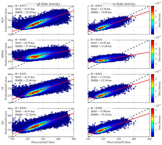
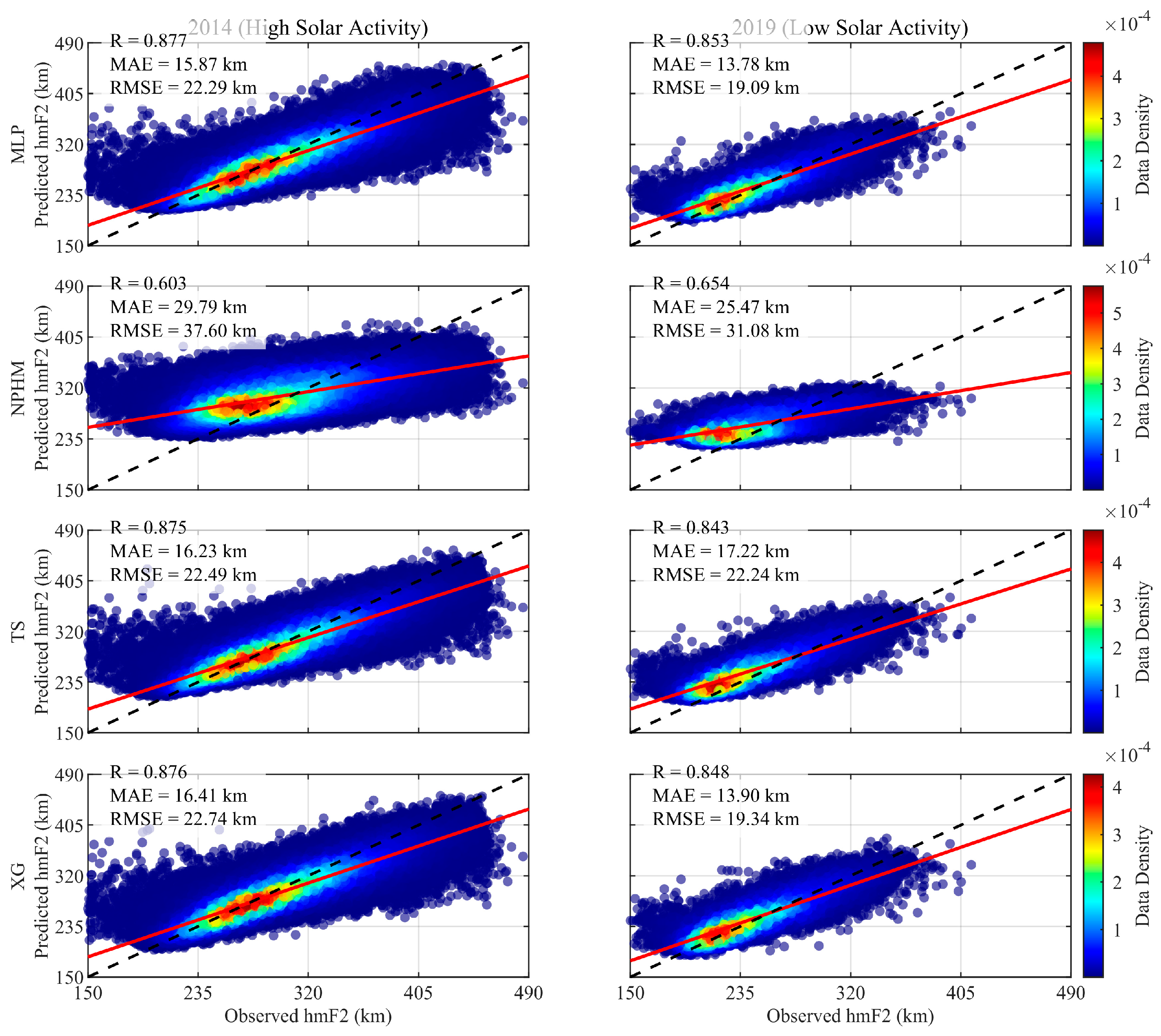
To compare the performance of each model, the hmF2 prediction results of the above models and the MLP model on the test set are analyzed together: with observed values as the horizontal axis and model-predicted values as the vertical axis, comparative scatter plots for the high-solar-activity year (2014) and low-solar-activity year (2019) are plotted (see Figure 5). The correlation coefficient (R), mean absolute error (MAE), and root mean squared error (RMSE) are selected as evaluation metrics to quantitatively assess the prediction accuracy of the five models, and the results are shown in Table 4.
Figure 5.
Density scatter plots of predictions from MLP, NPHM, Transformer and XGBoost.
Table 4.
Evaluation parameters of prediction accuracy for the four models (MLP, NPHM, TS, XG) based on hmF2 measurements from the COSMIC satellite in 2014 and 2019.
According to the evaluation results of the four models shown in Table 4, the prediction accuracy remains consistent overall, except that the correlation coefficient of the NPHM in 2019 is slightly higher than that in 2014. Specifically, the MLP model constructed in this study maintains the highest prediction accuracy in both years, with its correlation coefficient (R) reaching 0.877 and 0.853 respectively. Meanwhile, its mean absolute error (MAE) and root mean squared error (RMSE) are the lowest among all models—15.87 km and 22.29 km in 2014, and 13.78 km and 19.09 km in 2019. This indicates that the MLP model possesses stable and excellent regression prediction capabilities under different solar activity conditions.
From further analysis of the distribution characteristics of predicted values, when the observed hmF2 values in 2014 fall within the interval [200, 345] km, the scatter plot of the MLP model presents a narrow, highly extensible high-density belt distributed along the diagonal. This reflects that the model can maintain high prediction consistency and stability over a wide numerical range. In contrast, the high-density belts of the NPHM have significantly lower slopes, with shorter and broader distributions. This indicates that both models generally have a tendency to overestimate hmF2 in predictions, and the prediction deviation is more pronounced, especially in the high-value interval. This visual comparison further confirms the advantages of the MLP model in maintaining prediction accuracy and stability.
Compared with the Transformer (TS) model and XGBoost (XG) model, which also adopt machine learning methods, there is no significant difference in the overall morphology of the scatter plots between the MLP model and the two models—all three show concentrated diagonal distribution characteristics. However, in terms of quantitative evaluation indicators, the MLP model is slightly superior to the TS and XG models in terms of correlation coefficient, MAE, and RMSE. This indicates that while maintaining consistent overall prediction trends, the MLP model still has minor advantages in error control and prediction consistency. Overall, the MLP model not only achieves significant performance improvement compared with traditional empirical models but also demonstrates comparable or even better comprehensive prediction performance when compared with currently commonly used complex machine learning models. This verifies the effectiveness and robustness of the MLP model for high-precision hmF2 prediction under the feature and data conditions selected in this study.
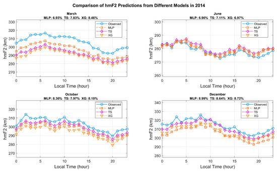
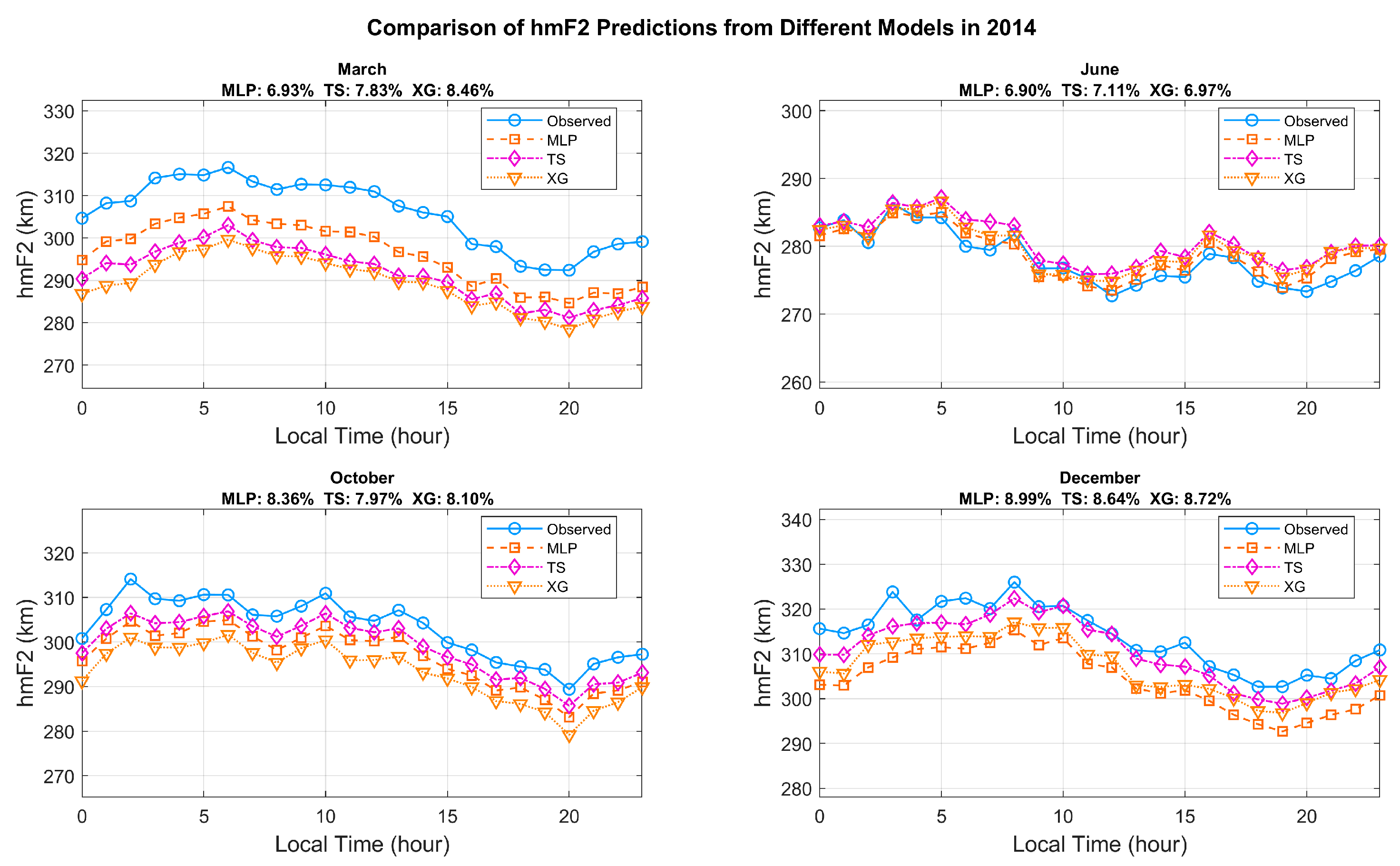
According to the variation relationship between predicted hmF2 values and Local Time (LT) in March, June, October, and December 2019 shown in Figure 6, the diurnal variation in hmF2 exhibits significant seasonal differences and diurnal periodicity under the background of low solar activity. The MLP model achieves the lowest Relative Root Mean Squared Error (RRMSE) across all selected months, with values of 7.31%, 6.42%, 7.09%, and 6.46%, respectively. These values are significantly lower than those of the comparative Transformer (TS) and XGBoost (XG) models.
Figure 6.
Schematic variation curves of prediction errors vs. Local Time (LT) for MLP, TS and XG models in March, June, October and December 2019.
While the TS and XG models demonstrate favorable prediction performance, their RRMSE values are generally higher than those of the MLP model. Notably, the TS model exhibits relatively higher RRMSE values of 8.87% in spring (March) and 8.46% in autumn (October). This indicates that its seasonal prediction stability is slightly inferior to that of the MLP model. In terms of the fitting degree between prediction curves and observed values, the MLP model’s predicted values closely align with the observed sequence throughout all time periods. This allows the MLP model to more accurately capture the diurnal variation patterns of hmF2.
Overall, the MLP model outperforms both the TS and XG models in predicting diurnal and seasonal hmF2 variations, as reflected by its consistently lower RRMSE. Moreover, it exhibits superior capability in capturing variation trends and maintaining prediction stability across different seasons. This further verifies the effectiveness and reliability of the MLP model in characterizing the complex spatiotemporal variations in ionospheric peak height. Compared with other machine learning approaches, the MLP model demonstrates stronger environmental adaptability and prediction robustness under challenging conditions such as low solar activity.
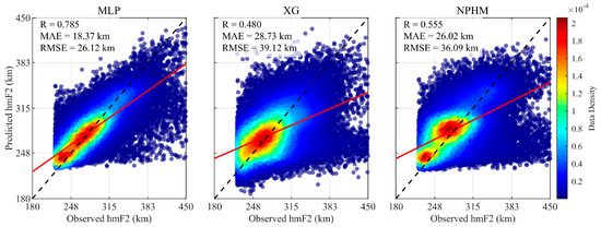
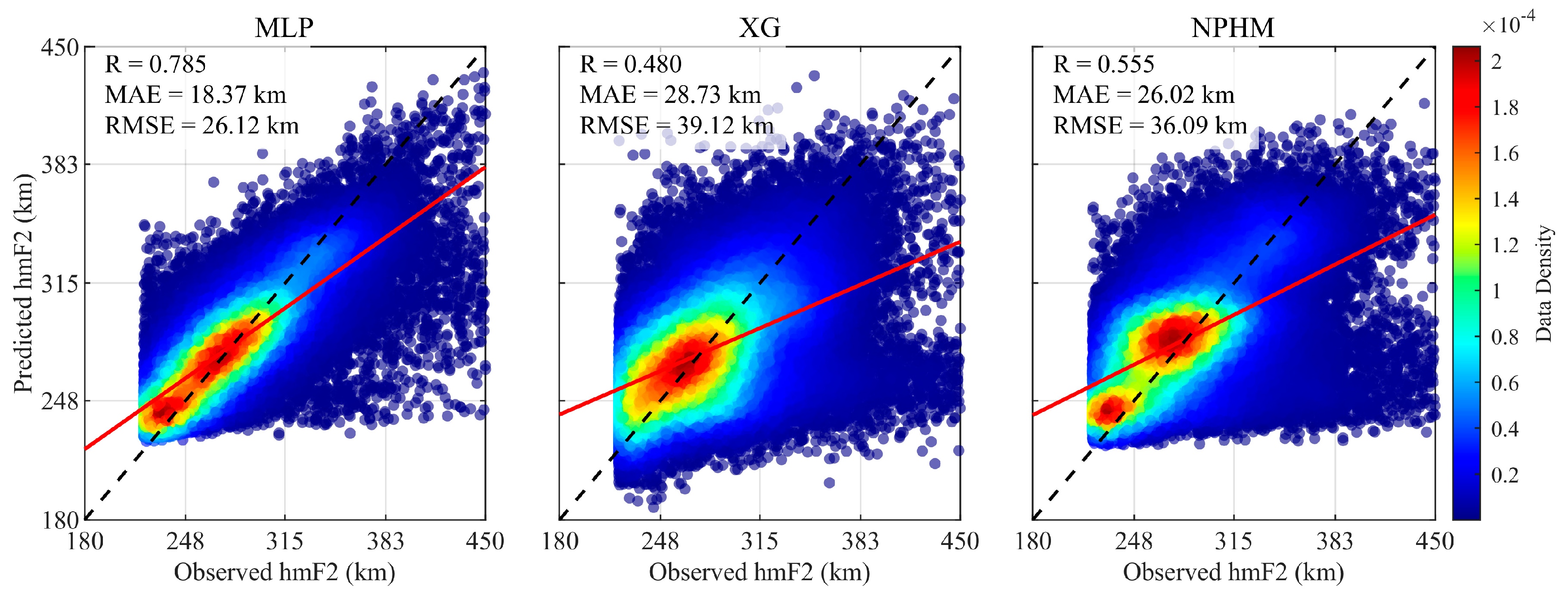
To verify the generalization performance of the model, this study constructed an independent validation set using a total of 50,000 observation data from the Global Ionospheric Radio Observatory (GIRO) network in 2014 and 2019. It should be emphasized that the training and evaluation of the MLP model are entirely based on COSMIC satellite radio occultation data, which covers high, middle, and low latitudes globally without regional bias. Therefore, the uneven geographical distribution of ground-based ionosonde stations (GIRO) does not affect the model’s global prediction accuracy. The independent test sets constructed from 2014 and 2019 COSMIC data provide an objective and unbiased assessment of the model’s global performance. Although the GIRO validation set has uneven spatial distribution, it is only used to verify the cross-data-source generalization ability of the model, rather than to evaluate the global prediction accuracy. This design ensures that the assessment of global hmF2 prediction accuracy is not affected by the limitation of ground-based station distribution. The MLP, XG, and NPHMs were employed to predict hmF2 under corresponding spatiotemporal conditions. Density scatter plots were drawn with GIRO observed values as the horizontal axis and model-predicted values as the vertical axis (see Figure 7), and the prediction accuracy evaluation indicators are presented in Table 5.
Figure 7.
Density scatter plots of predictions from MLP, XG, and NPHM.
Table 5.
Prediction accuracy evaluation parameters of the three models (MLP, XG, NPHM) for hmF2 measurements from GIRO in 2014 and 2019.
According to the prediction accuracy evaluation parameters of the four models for hmF2 observations from GIRO stations in 2014 and 2019 listed in Table 5, the MLP model exhibits significant advantages in all indicators: its correlation coefficient (R) reaches 0.785, with a mean absolute error (MAE) of 18.37 km and a root mean squared error (RMSE) of 26.12 km, which are significantly superior to those of the XG model and NPHM. This result indicates that in the prediction task based on ground station data, the MLP model can more accurately capture the variation trends of hmF2 with the minimum overall prediction error.
Further analysis of the morphology of the prediction density scatter plots shown in Figure 7 reveals that the high-density belt of the MLP model presents a narrow and extended shape, distributed along the diagonal. This reflects that the model can maintain high prediction consistency and stability over a wide numerical range. In contrast, the high-density belts of the XG model and NPHMs all show an obviously thick and short distribution. Specifically, the NPHM even has two separated high-density centers, suggesting the existence of certain systematic deviations or modal splitting in its predictions. In addition, the overall slope of the MLP scatter plot is closer to 1, indicating a better linear correspondence between its predicted values and observed values, which further confirms its superiority in trend restoration.
Based on the above quantitative indicators and visual analysis results, the MLP model not only has lower statistical errors than other comparative models but also demonstrates significant advantages in prediction stability, consistency, and trend restoration effect. This further verifies the strong adaptability and reliability of the MLP model in ionospheric peak height modeling, especially in the application scenario of ground station data, providing an effective machine learning solution for high-precision hmF2 prediction.
5. Model Interpretability Analysis
5.1. Interpretability Analysis of the Prediction Model
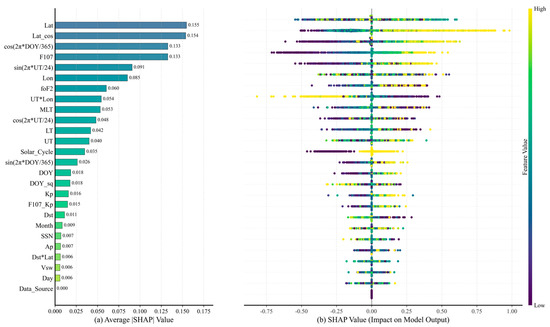
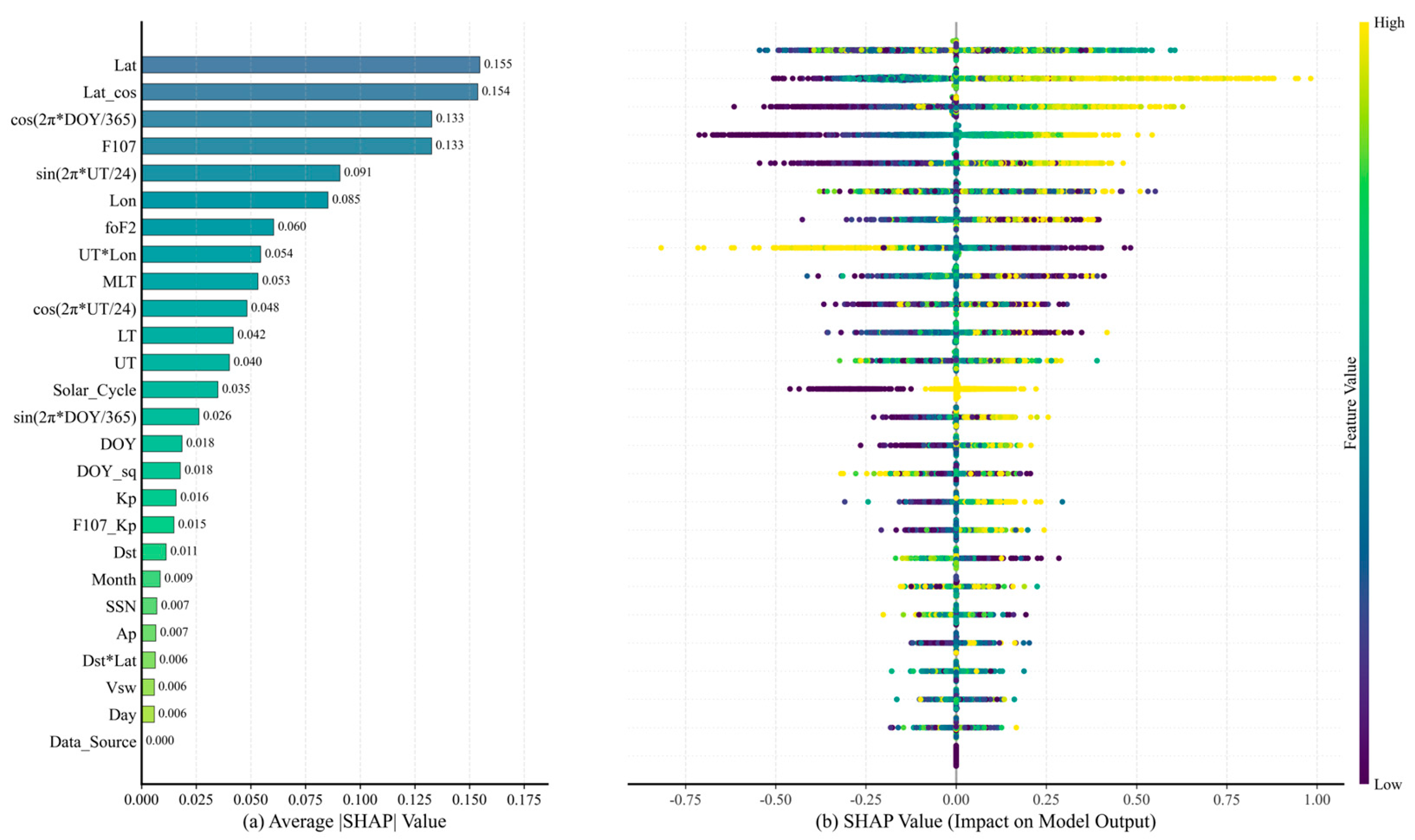
Figure 8a is the feature importance ranking plot, and Figure 8b is the swarm plot. In Figure 8a, the horizontal axis represents the mean absolute SHAP values. In Figure 8b, the horizontal axis denotes the SHAP values, the vertical axis represents the global feature importance ranking, and the color mapping reflects the magnitude of feature values—blue indicates low values and yellow indicates high values.
Figure 8.
Feature importance analysis (a) bar chart on the left: average absolute SHAP value of features and their relative contribution percentages; (b) beeswarm plot on the right: SHAP value distribution, with the color of the dots indicating the feature value. Features are sorted in descending order of importance.
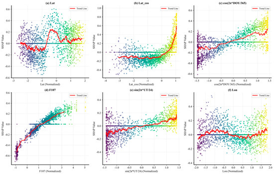
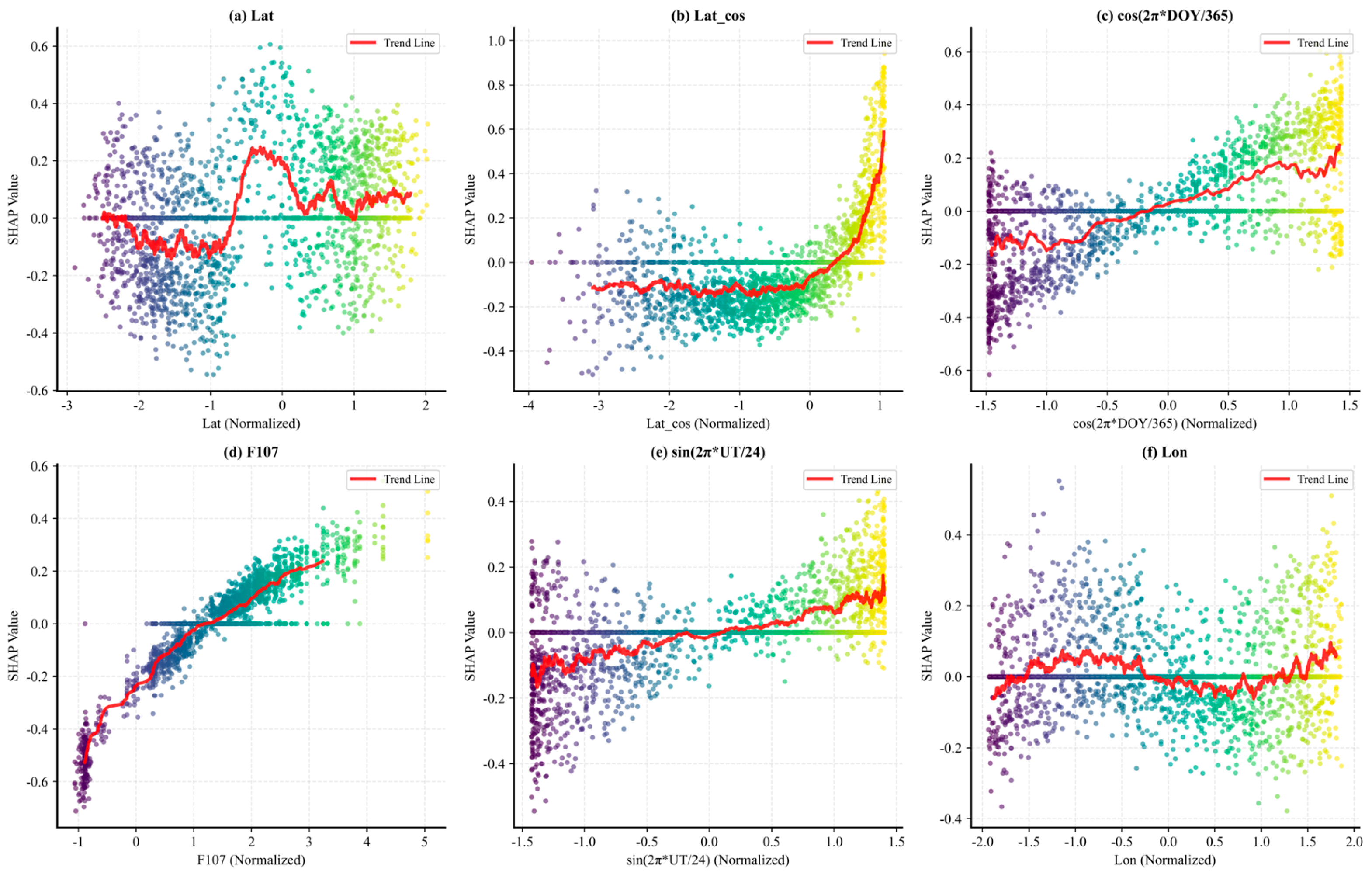
Feature importance analysis based on the SHAP (v0.42.1, https://shap.readthedocs.io/, accessed 12 March 2026) (SHapley Additive exPlanations) method provides an interpretable perspective for deciphering the decision-making mechanism of the MLP model in hmF2 prediction. As shown in Figure 8 and Figure 9, this study systematically evaluated the contribution and influence pattern of each input feature on the model’s prediction results by calculating the SHAP values of test set samples. The analysis results indicate that the model’s predictions are mainly co-driven by spatial position parameters and solar activity indices.
Figure 9.
Feature dependence plots of standardized values and SHAP values for the top 6 features by mean absolute SHAP values.
The feature importance ranking reveals that latitude and its cosine transformation are the core factors affecting hmF2 prediction, with their mean absolute SHAP values reaching 0.155 and 0.154, respectively, which are significantly higher than those of other features. This highlights the typical distribution characteristics of hmF2 varying with geographic latitude, embodying the core laws of ionospheric morphology. Followed by the annual periodic term and F10.7 solar radio flux index, both with a mean absolute SHAP value of 0.133, indicating that changes in solar radiation intensity and seasonal effects caused by Earth’s revolution exert nearly equally important regulatory effects on hmF2. The diurnal periodic term and longitude also rank among the top six important features, confirming the diurnal variation law of hmF2 and its potential geographic longitude dependence. The non-negligible importance of UT × Lon, with a mean absolute SHAP value of 0.060, further verifies that the longitudinal modulation effect caused by Earth’s rotation is a key spatiotemporal feature regulating the global distribution of hmF2, which also proves the rationality of introducing LT, UT and Lon as independent input parameters.
Further insights into the influence of feature value magnitude on prediction direction can be gained from the SHAP swarm plot (Figure 8b). For the core feature of latitude, its high values are mainly distributed in the positive SHAP value region, while low values are concentrated in the negative SHAP value region. This means the model determines that lower latitudes tend to increase the predicted hmF2 value, while higher latitudes tend to decrease it, which is consistent with the physical characteristics of the ionospheric equatorial anomaly hump region. The latitude cosine and F10.7 index exhibit a similar pattern: high feature values are strongly correlated with positive SHAP values and low values with negative SHAP values. Moreover, the amplitude of positive SHAP values is generally larger than that of negative ones, indicating that these features in high-value states contribute more significantly to improving prediction results.
In-depth analysis of the SHAP dependence plots of key features can reveal the specific functional form of their impact on predictions. The dependence plot of latitude and SHAP values presents an approximate pulse-like distribution: SHAP values of samples in the Southern Hemisphere are mainly negative, those in the Northern Hemisphere are mainly positive, and a peak appears near the equator. This clearly quantifies the hemispheric asymmetry in the formation mechanism of hmF2. The dependence plot of latitude cosine shows that when its standardized value is less than 0.5, the SHAP value is basically negative; when it exceeds 0.5, the SHAP value turns positive with a steep change curve, reaffirming the positive dominant role of low-latitude regions in hmF2. The dependence relationship of the F10.7 index exhibits segmental characteristics: when the standardized F10.7 value is less than 0 (period of extremely weak solar activity), the SHAP value is stably distributed in the interval [−0.6, −0.4], and its absolute value is significantly higher than that in periods of higher solar activity. The trend line at this stage is nearly parallel to the vertical axis, indicating that during extremely weak solar activity, minor changes in the F10.7 index have a relatively constant negative inhibitory effect on hmF2 prediction. After entering the period of higher solar activity, the SHAP value increases approximately linearly with the growth of the F10.7 index, rising from about −0.2 to around 0.5, revealing that the dominant role of enhanced solar radiation in lifting the ionospheric peak height becomes significantly prominent. This transition characteristic indicates that the model captures the nonlinear threshold characteristic of hmF2’s response to solar activity—only when solar activity exceeds a specific level does its enhancement exert a strong positive driving effect on hmF2.
In summary, SHAP analysis not only quantifies the relative importance of each feature to the MLP model’s hmF2 prediction from a global perspective (the top six features contribute more than 70% of the influence) but also depicts the complex nonlinear relationships between key features and prediction results through dependence plots. These findings are highly consistent with ionospheric physical cognition, which not only improves the credibility and interpretability of the constructed machine learning model but also verifies from a data-driven perspective that latitude, solar activity, and periodic changes are the primary factors regulating the spatiotemporal evolution of hmF2.
5.2. Feature Ablation Experiment
To verify the scientificity and non-redundancy of the feature design, this study conducted feature ablation experiments on the 2014 and 2019 COSMIC test sets. The feature zeroing method was used to mask the questioned features in gradient. RMSE, MAE and Pearson correlation coefficient R were used to quantify the performance, so as to verify the actual contribution of each feature group to the model.
5.2.1. Experimental Design
The experiment included one full-feature baseline experiment and five gradient masking experiments, with data strictly limited to the 2014 and 2019 COSMIC test sets. The specific settings were as follows: (1) baseline: using all constructed features; (2) masking solar activity feature SSN; (3) masking geomagnetic activity feature Ap; (4) masking time features month/day/UT; (5) masking composite interaction features F107_Kp/UT × Lon/Dst × Lat; and (5) fully masking all questioned redundant or composite features.
5.2.2. Experimental Results and Analysis
Table 5 shows the performance comparison results of the six groups of experiments. ΔRMSE and ΔR are the change values relative to the baseline, and positive values indicate increased error or decreased correlation.
5.2.3. Result Analysis
The experimental results presented in Table 6 quantitatively demonstrate the non-redundancy and necessity of the proposed feature set. Different types of feature masking lead to distinct degrees of model performance degradation, which fully verifies the rationality of the physics-guided feature engineering strategy.
Table 6.
Performance comparison of feature ablation experiments on 2014 and 2019 test set data.
Specifically, masking the temporal features (month, day, UT) results in a significant performance drop: RMSE increases from 22.0 km to 34.1 km and the correlation coefficient R decreases from 0.889 to 0.703. This indicates that the temporal information encoded by month, day, and UT is crucial for capturing the diurnal and seasonal variation patterns of hmF2 and cannot be replaced by other features alone.
Furthermore, removing the composite interaction features (F107_Kp, UT × Lon, Dst × Lat) leads to an RMSE increase of 31.7% and an R decrease of 10.8%. This validates that these composite terms effectively capture the nonlinear physical coupling effects in the ionosphere, which are critical for improving the model’s ability to simulate complex ionospheric disturbances.
Notably, masking individual features such as SSN or Ap has no significant impact on model performance, indicating that these features provide redundant information under the current feature set, and their roles can be compensated by other core features (e.g., F10.7 index). However, fully masking all questioned redundant and composite features causes catastrophic performance degradation: RMSE surges by 95.1% and R drops by 44.5%, which further confirms that the majority of the constructed features are non-redundant and indispensable for high-precision hmF2 prediction.
6. Conclusions
In this study, a global prediction model for the peak height of the ionospheric F2 layer (hmF2) was constructed based on the Multilayer Perceptron (MLP). Systematic training, evaluation, and comparative analysis of the model were performed by comprehensively utilizing COSMIC occultation data and GIRO ground-based observation data. The results demonstrate that the model exhibits excellent predictive capability and stability: on the test sets of 2014 and 2019, the correlation coefficients (R) between the predicted values and observed values reached 0.877 and 0.853, respectively, with root mean square errors (RMSE) of 22.29 km and 19.09 km. The key findings of this study are summarized as follows:
(1) The distribution characteristics of prediction errors reflect the model’s performance under different ionospheric states. The mean value of the prediction errors shows a negative bias, and the standard deviation indicates a certain degree of error dispersion. The error distribution presents a leptokurtic and left-skewed pattern, which suggests that the model can achieve accurate and stable predictions for quiet or normal ionospheric states, while predictions of severe disturbance events constitute the primary source of errors. In addition, the model successfully reproduces the global hmF2 distribution pattern dominated by physical mechanisms such as thermospheric circulation and equatorial electrodynamics. The consistency between the prediction results and well-established physical laws further verifies the model’s physical rationality and generalization capability.
(2) The MLP model demonstrates comprehensive and stable accuracy advantages across multiple core evaluation metrics. In the comparative tests of high- and low-solar-activity years, the MLP model consistently outperforms other comparative models in three indicators, namely correlation coefficient (R), mean absolute error (MAE), and root mean square error (RMSE). Particularly in the generalization test on the independent GIRO validation set, the density scatter plot of the MLP model’s predictions presents a narrow distribution extending along the diagonal, which intuitively reflects its small prediction bias and high consistency. In contrast, the scatter distributions of other models are relatively broad and dispersed, and some even exhibit multi-center separation characteristics.
(3) The model exhibits excellent generalization capability and cross-data-source adaptability. The model trained on COSMIC satellite data maintains high prediction accuracy on GIRO ground-based observation data that were not involved in training, with a correlation coefficient (R) of 0.785, an RMSE of 26.1 km, and an MAE of 18.4 km. This performance is significantly superior to that of the NPHM and the XGBoost model. This indicates that the model can be effectively transferred to data scenarios from different observation platforms and possesses robust predictive capability independent of specific data sources.
(4) The interpretability analysis based on SHAP (SHapley Additive exPlanations) quantitatively reveals the core physical features driving hmF2 prediction and their action mechanisms. The analysis results show that latitude and its cosine transformation, the F10.7 solar radio flux index, and harmonic terms representing annual and diurnal cycles are the top five key factors affecting model predictions, with their mean absolute SHAP values of 0.155, 0.154, 0.133, 0.133, and 0.091, respectively. Further dependence analysis indicates that the impact of latitude on hmF2 presents a significant north–south hemispheric asymmetry; in contrast, the impact of the F10.7 index exhibits an obvious nonlinear threshold effect—it exerts a stable inhibitory effect on hmF2 during low-solar-activity periods, and shifts to a significant linear lifting effect in high-solar-activity periods.
In summary, the MLP-hmF2 prediction model constructed in this study demonstrates significant advantages in prediction accuracy, cross-data-source robustness, physical interpretability, and computational efficiency. For the 5256 global prediction samples in Figure 4, the pure inference time of the model is only 0.054 s, providing an efficient solution for rapid global hmF2 prediction. This model not only provides a high-precision and reliable technical tool for the nowcasting and forecasting of ionospheric space weather and radio communication applications, but also offers new quantitative evidence for deepening the understanding of the spatiotemporal evolution law of ionospheric peak height through the key features and impact mechanisms revealed by SHAP analysis. In addition, the model’s stable performance across both high- and low-solar-activity years particularly improves the reliability of ionospheric parameter prediction under low-solar-activity conditions, indicating considerable potential for operational applications.
Feature ablation experiments further consolidated the foundation of the model. The results highlighted the critical role of global spatiotemporal parameters (UT, Lon) and physics-based composite features in improving prediction accuracy
Despite the satisfactory performance of the proposed MLP model, we acknowledge certain limitations in the current feature selection strategy that warrant further investigation. First, the simultaneous inclusion of F10.7 and sunspot number (SSN) may introduce multicollinearity, as both are closely correlated proxies of solar activity. Although SHAP analysis suggested that they contribute complementary information in the current setting, future work will incorporate formal multicollinearity diagnostics (e.g., variance inflation factor) and systematic feature selection techniques to construct a more robust and non-redundant input set. Second, the deterministic linear relationship among Universal Time (UT), Local Time (LT), and longitude (Lon) implies that only two of these three variables are mathematically independent. While each parameter carries distinct physical relevance—UT as a global time reference, LT representing local solar time, and Lon capturing longitudinal variations—their interdependence suggests that including all three may lead to redundancy. Subsequent studies will explore the use of independent variable combinations (e.g., UT + Lon or LT + Lon) to ensure a theoretically sound and parsimonious feature space. Addressing these methodological aspects will further enhance the reliability, interpretability, and generalizability of hmF2 prediction models.
Author Contributions
Conceptualization, M.O.; methodology, F.W.; software, F.W.; validation, Q.Z. and J.L.; formal analysis, L.C.; investigation, X.C.; resources, Y.Z.; data curation, F.W.; writing—original draft preparation, F.W.; writing—review and editing, M.O.; visualization, B.Z.; supervision, M.O.; project administration, Q.Z.; funding acquisition, M.O. All authors have read and agreed to the published version of the manuscript.
Funding
This research was funded by the National Key R&D Program of China (Grant No. 2022YFF0503900) and the Stable Support Project for National Field Observation Stations (Grant No. A250106150). The latter supported the revision of this manuscript.
Institutional Review Board Statement
Not applicable.
Informed Consent Statement
Not applicable.
Data Availability Statement
COSMIC and GRACE data can primarily be obtained from CDAAC (https://data.cosmic.ucar.edu/gnss-ro (accessed from 1 January 2007 to 31 December 2023)). GIRO data is available for bulk download at https://lgdc.uml.edu (accessed from 1 January 2007 to 31 December 2023). Solar activity and geomagnetic activity data can be accessed through the following link: https://omniweb.gsfc.nasa.gov/form/dx1.html (accessed from 1 January 2007 to 31 December 2023).
Acknowledgments
We sincerely acknowledge the valuable guidance from our supervisors and helpful discussions with laboratory colleagues during the research. We also thank the providers of COSMIC and GIRO datasets for laying the foundation of this study. During the preparation of this manuscript, the authors used DeepSeek (https://www.deepseek.com/, accessed 12 March 2026) and Doubao (https://www.doubao.com/, accessed 12 March 2026) for Chinese manuscript polishing and English translation; the authors have reviewed and edited the output and take full responsibility for the content of this publication.
Conflicts of Interest
The funders had no role in the design of the study; in the collection, analyses, or interpretation of data; in the writing of the manuscript; or in the decision to publish the results.
Abbreviations
The following abbreviations are used in this manuscript:
| IRI | International Reference Ionosphere |
| XG | eXtreme Gradient Boosting |
| SHAP | SHapley Additive exPlanation |
| NPHM | Neustrelitz Peak Height Model |
| TS | Transformer |
References
- Lin, Z.Y.; Chen, L.J.; Jin, R.M.; Ou, M.; Yang, H.; Ji, G.; Cui, X.; Gu, M. Ionospheric foF2 Prediction Model over China and Surrounding Regions Based on Random Forest Algorithm. Glob. Position. Syst. 2024, 49, 88–96. [Google Scholar]
- Song, B.H. Accuracy Evaluation of Ionospheric Forecasting Based on BP Neural Network Model. Glob. Position. Syst. 2023, 48, 79–82, 102. [Google Scholar]
- Zhu, J.H.; Yan, W.L.; Jin, Y.F.; Yan, T.; Wang, J. Comparative Analysis of Four Neural Network Methods for TEC Modeling During Ionospheric Magnetic Storm Periods. Chin. J. Space Sci. 2025, 45, 1230–1242. [Google Scholar] [CrossRef] [Scilit]
- Pan, L.; Wu, X. Precipitation Nowcasting Model Based on Bidirectional Transformer. Appl. Res. Comput. 2024, 41, 2455–2460. [Google Scholar]
- Sun, F.F.; Luo, J. Performance Evaluation of the hmF2 Parameter in the Ionospheric Model IRI-2016. J. Geomat. 2019, 44, 82–86. [Google Scholar]
- Moses, M.; Bilitza, D.; Panda, S.K.; Ochonugor, B.J. Assessment of IRI-2016 hmF2 Model Predictions with COSMIC Observations over the African Region. Adv. Space Res. 2021, 68, 2115–2123. [Google Scholar] [CrossRef] [Scilit]
- Wang, J.; Yu, Q.; Shi, Y. Comparison of Observed hmF2 and the IRI-2020 Model for Six Stations in East Asia During the Declining Phase of Solar Cycle 24. Adv. Space Res. 2024, 73, 2418–2432. [Google Scholar] [CrossRef] [Scilit]
- Sai Gowtam, V.; Tulasi Ram, S. An Artificial Neural Network-Based Ionospheric Model to Predict NmF2 and hmF2 Using Long-Term Data Set of FORMOSAT-3/COSMIC Radio Occultation Observations: Preliminary Results. J. Geophys. Res. Space Phys. 2017, 122, 11743–11755. [Google Scholar] [CrossRef] [Scilit]
- Mushi, E.P.; Sulungu, E.D.; Pamain, A. Prediction of F2-Layer Height of the Peak Electron Density (hmF2) Over the Southern Africa Region Using Artificial Neural Network. East Afr. J. Sci. Technol. Innov. 2024, 6. [Google Scholar] [CrossRef] [Scilit]
- Akhoondzadeh, M. A MLP Neural Network as an Investigator of TEC Time Series to Detect Seismo-Ionospheric Anomalies. Adv. Space Res. 2013, 51, 2048–2057. [Google Scholar] [CrossRef] [Scilit]
- Wang, J.; Yu, Q.; Shi, Y.; Yang, C. A Prediction Method of Ionospheric hmF2 Based on Machine Learning. Remote Sens. 2023, 15, 3154. [Google Scholar] [CrossRef] [Scilit]
- Liu, F.T.; Ting, K.M.; Zhou, Z.H. Isolation Forest. In Proceedings of the 8th IEEE International Conference on Data Mining; IEEE: Piscataway, NJ, USA, 2008; pp. 413–422. [Google Scholar]
- Chen, T.; He, T.; Benesty, M.; Khotilovich, V.; Tang, Y.; Cho, H.; Chen, K.; Mitchell, R.; Cano, I.; Zhou, T.; et al. Xgboost: Extreme Gradient Boost, R Package Version 0.4-2; Distributed (Deep) Machine Learning Community: Washington, DC, USA, 2015.
- Bahdanau, D.; Cho, K.; Bengio, Y. Neural Machine Translation by Jointly Learning to Align and Translate. arXiv 2014, arXiv:1409.0473. [Google Scholar] [CrossRef] [Scilit]
- Yoon, K.; Dyer, C.; Luong, H.; Rush, A.M. Structured Attention Networks. In Proceedings of the International Conference on Learning Representations, Toulon, France, 24–26 April 2017. [Google Scholar]
- Vaswani, A.; Shazeer, N.; Parmar, N.; Uszkoreit, J.; Jones, L.; Gomez, A.; Kaiser, Ł.; Polosukhin, I. Attention Is All You Need. arXiv 2017, arXiv:1706.03762. [Google Scholar] [CrossRef] [Scilit]
- Rumelhart, D.E.; Hinton, G.E.; Williams, R.J. Learning Representations by Back-Propagating Errors. Nature 1986, 323, 533–536. [Google Scholar] [CrossRef] [Scilit]
- Hornik, K.; Stinchcombe, M.; White, H. Multilayer Feedforward Networks Are Universal Approximators. Neural Netw. 1989, 2, 359–366. [Google Scholar] [CrossRef] [Scilit]
- Narayanan, R.; Ganesh, N. A Comprehensive Review of Metaheuristics for Hyperparameter Optimization in Machine Learning. In Metaheuristics for Machine Learning: Algorithms and Applications; Wiley: Hoboken, NJ, USA, 2024; pp. 37–72. [Google Scholar]
- Smith, L.N. Cyclical Learning Rates for Training Neural Networks. In Proceedings of the 2017 IEEE Winter Conference on Applications of Computer Vision; IEEE: Piscataway, NJ, USA, 2017; pp. 464–472. [Google Scholar]
- Huber, P.J. Robust Estimation of a Location Parameter. In Breakthroughs in Statistics: Methodology and Distribution; Springer: New York, NY, USA, 1992; pp. 492–518. [Google Scholar]
- Lundberg, S.M.; Nair, B.; Vavilala, M.S.; Horibe, M.; Eisses, M.J.; Adams, T.; Liston, D.E.; Low, D.K.-W.; Newman, S.-F.; Kim, J.; et al. Explainable Machine-Learning Predictions for the Prevention of Hypoxaemia During Surgery. Nat. Biomed. Eng. 2018, 2, 749–760. [Google Scholar] [CrossRef] [Scilit] [PubMed]
- Lundberg, S.M.; Lee, S.I. A Unified Approach to Interpreting Model Predictions. arXiv 2017, arXiv:1705.07874. [Google Scholar] [CrossRef] [Scilit]
- Karpachev, A.T.; Gasilov, N.A. Variations of the Vertical Plasma Drift with Longitude in the Midlatitude Nighttime Summer Ionosphere Deduced from Measurements of hmF2. Geomagn. Aeron. 1998, 38, 617. [Google Scholar]
- Li, B.; Cui, R.F.; Weng, L.B. Seasonal Variations of Global Ionospheric Peak Parameters. Chin. J. Space Sci. 2024, 44, 60–70. [Google Scholar] [CrossRef] [Scilit]
- Burns, A.G.; Solomon, S.C.; Wang, W.; Jee, G.; Lin, C.H.; Rocken, C.; Kuo, Y.H. The Summer Evening Anomaly and Conjugate Effects. J. Geophys. Res. Space Phys. 2011, 116. [Google Scholar] [CrossRef] [Scilit]
- Oyekola, O.S. Evening and Nighttime Features of Equatorial Ionospheric F2 Layer. In Proceedings of the 41st COSPAR Scientific Assembly, Istanbul, Turkey, 30 July–7 August 2016; pp. 1–54. [Google Scholar]
- Yu, T.; Wan, W.X.; Liu, L.B.; Mao, T.; Wang, Y.G.; Wang, J.S. Annual and Semiannual Variations of Peak Parameters in the Ionospheric F2 Layer at Mid-Low Latitudes and Simulation of Electric Field Effects. Sci. Technol. Rev. 2008, 26, 25–30. [Google Scholar]
- Hoque, M.M.; Jakowski, N. A New Global Model for the Ionospheric F2 Peak Height for Radio Wave Propagation. Ann. Geophys. 2012, 30, 797–809. [Google Scholar] [CrossRef] [Scilit]

Disclaimer/Publisher’s Note: The statements, opinions and data contained in all publications are solely those of the individual author(s) and contributor(s) and not of MDPI and/or the editor(s). MDPI and/or the editor(s) disclaim responsibility for any injury to people or property resulting from any ideas, methods, instructions or products referred to in the content. |
© 2026 by the authors. Licensee MDPI, Basel, Switzerland. This article is an open access article distributed under the terms and conditions of the Creative Commons Attribution (CC BY) license.