Article

A System-Based Assessment of Methane Sources in an Eastern European Urban Environment (Cluj-Napoca, Romania)


Faculty of Environmental Science and Engineering, Babeș-Bolyai University, 400294 Cluj-Napoca, Romania
*
Author to whom correspondence should be addressed.
Atmosphere 2026, 17(4), 351; https://doi.org/10.3390/atmos17040351
Submission received: 27 February 2026 / Revised: 25 March 2026 / Accepted: 28 March 2026 / Published: 31 March 2026
(This article belongs to the Section Air Quality)

Abstract

Methane (CH4) emissions in urban areas remain a major source of uncertainty in greenhouse gas inventories, particularly in Eastern European cities, where observational studies are limited. This study presents a comprehensive, system-based assessment of CH4 sources in Cluj-Napoca, Romania, based on high-resolution in situ measurements across five representative urban systems: aquatic environments (AQs), natural gas distribution end-use points (NG), sewer infrastructure (SE), building basements (BSs), and traffic emissions (TEs). Elevated CH4 concentrations were consistently detected across all investigated systems, confirming the coexistence of both diffuse and point sources within the urban environment. Dissolved methane (dCH4) in aquatic systems showed strong and persistent oversaturation relative to atmospheric equilibrium, reaching up to 3 × 10⁵% of air–water equilibrium, indicating active microbial methanogenesis enhanced by urban inputs of organic matter and nutrients. Measurements at natural gas end-use points revealed highly localized leaks with concentrations up to 482 ppmv. Sewer infrastructure exhibited extreme variability (up to 1222 ppmv), likely controlled by a combination of microbial production, hydraulic conditions, and potential interactions with adjacent gas distribution networks. Basement environments showed CH4 accumulation up to 12 ppmv, reflecting the combined effects of gas leakage and limited ventilation. Measurements at vehicle exhausts identified transient CH4 peaks reaching 162 ppmv during vehicle engine acceleration, with distinct ethane-to-methane ratios, indicative of pyrogenic sources. Overall, these results demonstrate that urban CH4 emissions are spatially heterogeneous, temporally variable, and derived from multiple coexisting sources. The urban area should, therefore, be understood as a hybrid environment, with natural and anthropogenic CH4 contributions.

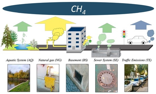
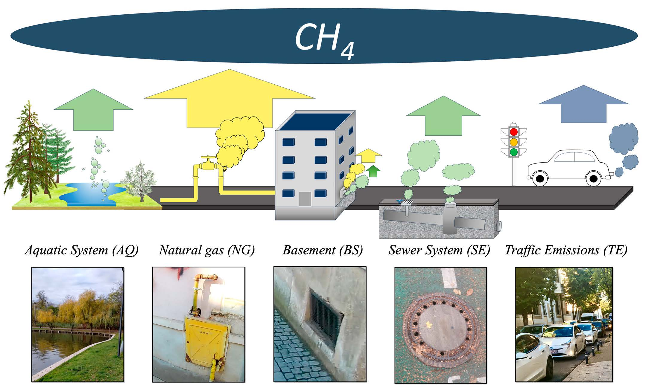
Graphical Abstract

1. Introduction

Climate change, driven by increasing concentrations of greenhouse gases (GHGs), has raised the global mean land–ocean surface temperature by 0.65–1.06 °C between 1880 and 2012, and the temperature modification is expected to exceed 2 °C by the end of the 21st century [1]. International frameworks such as the United Nations Framework Convention on Climate Change (UNFCCC), the Kyoto Protocol, and the Paris Agreement have established coordinated strategies for reducing GHG emissions and enhancing transparency in emission reporting [2]. Within the European Union (EU), policy instruments, including the European Green Deal and the European Climate Law, commit member states to reducing GHG emissions by at least 55% by 2030 and to achieving carbon neutrality by 2050 [3]. These commitments emphasize the need for robust GHG inventories and accurate quantification of emissions from all sectors, including those that remain poorly constrained.
Methane (CH4), the second most significant greenhouse gas (GHG) after carbon dioxide (CO2), is increasingly recognized as a priority mitigation target due to its short atmospheric lifetime (~12 years) and strong radiative efficiency, as its global warming potential is 86 times that of CO2 over a 20-year horizon and 28 times over a 100-year horizon [2,4].
The global mean methane concentration has risen from ~722 ppbv in 1750 [5] to ~1940 ppbv in 2025 [6]. Methane reduction can yield rapid climate benefits—a 45% cut by 2030 could reduce near-term warming by ~0.3 °C [7]. Thus, CH4 mitigation represents one of the most effective near-term levers for achieving global temperature stabilization.
Atmospheric methane originates from three primary production pathways—biogenic, thermogenic, and pyrogenic—and from both natural and anthropogenic processes [2,4]. Biogenic CH4 is generated through methanogenesis under anaerobic conditions in wetlands, aquatic sediments, and the digestive system of ruminants. Thermogenic CH4 forms via the thermal decomposition of organic matter in fossil reservoirs, which may reach the atmosphere through natural seeps or anthropogenic extraction and distribution of fossil fuels. Pyrogenic CH4 results from the incomplete combustion of biomass and biofuels.
Natural sources include wetlands (~40% of overall CH4 emissions), inland waters, termites, oceans, and thawing permafrost [2,4]. Anthropogenic activities account for roughly 60% of global CH4 emissions, mainly from fossil fuel extraction and distribution, agriculture, and waste management [4]. The major atmospheric sink is oxidation by hydroxyl radicals (OH) in the troposphere (~90% of the global CH4 loss), complemented by stratospheric oxidation and microbial uptake in soils [2,4]. However, land-use changes and urbanization can disrupt soil physiochemical properties and microbial communities, suppressing methanotrophic activity and thus weakening the terrestrial CH4 sink [8,9].
Although urban areas occupy only ~2% of the Earth’s surface, they host more than half of the global population [10,11] and contribute disproportionately to global GHG emissions. Rapid urban expansion intensifies energy consumption, infrastructure development and transportation—all of which can raise the CH4 emissions. Yet, the spatial and temporal complexity of urban systems, coupled with limited direct observations, introduces large uncertainties in quantifying urban CH4 budgets [1,11]. Persistent discrepancies between bottom-up (inventory-based) and top-down (atmospheric) estimates highlight systematic underestimation of fugitive emissions, particularly from natural gas networks [12,13,14].
Urban-based studies, including high-frequency in situ sensors, mobile surveys, and isotopic or co-emitted tracers, have stated that methane emissions in urban areas originate from diverse sources, both anthropogenic and natural, including: agricultural and biomass burning activities [15,16,17]; urban aquatic systems such as rivers, ponds, and lakes [18,19,20,21,22,23]; landfills and waste management sites [24,25,26,27]; natural gas distribution networks [13,28,29,30]; oil and gas production [31,32,33]; sewage systems and wastewater treatment plants [27,33,34,35,36,37,38,39]; and vehicle exhausts and traffic emissions, particularly from NG-powered vehicles [40,41,42,43].
However, despite numerous urban-based studies in North America [26,29,30,33,44,45,46,47,48,49,50,51] and Western Europe [13,16,17,52,53,54,55,56,57,58], there is still a gap in Eastern Europe, particularly in Romania, where urban CH4 research is limited primarily to Bucharest [13,59]. In Cluj-Napoca, some early studies have investigated CH4 emissions from municipal landfills [60,61].
Understanding urban methane budgets requires resolving emission dynamics across multiple spatial and temporal scales. In Cluj-Napoca, a three-phase observational framework has been implemented to bridge CH4 atmospheric signals with their underlying point-source environments. First, an eight-month continuous stationary atmospheric monitoring campaign, combined with isotopic analyses (δ13C-CH4 and δ2H-CH4), provided integrated city-scale CH4 signals, published by van Es et al. [62]. By incorporating wind speed, wind direction, and diurnal variability, this approach identified dominant source sectors and revealed the intersecting influence of thermogenic and biogenic emissions on the urban atmosphere. The isotopic signature enabled methane source classification and highlighted the complexity of overlapping urban signatures. Second, a street-level walking approach (Hmoudah & Baciu, under review) mapped localized CH4 enhancements along the urban road network. This mobile approach facilitated the detection of fugitive emissions from the natural gas distribution network. While these approaches effectively characterized atmospheric patterns and identified concentration anomalies, they did not directly resolve the specific urban systems contributing to the urban methane budget.
To address this gap, the present study applies a systematic, direct, high-resolution point-source investigation to differentiate CH4 concentration variability and source distribution across five major urban systems: (i) urban aquatic systems (AQs), (ii) natural gas distribution grid and end-use points (NG), (iii) sewer infrastructure (SE), (iv) building basements (BSs), and (v) traffic-related emissions (TEs). These systems represent the principal anthropogenic and biogenic components shaping the urban methane dynamics.
Although flux quantification is beyond the scope of this study, the focus on direct CH4 detection and spatial leak identification provides mechanistic insight to better understand emission heterogeneity and source attribution within a complex urban setting.
By integrating field-based direct observations with previous atmospheric and street-level investigations, this study achieves a multi-scale methane assessment framework for Cluj-Napoca. The findings improve understanding of urban CH4 emission in underrepresented Eastern European contexts, and therefore, they are expected to guide further investigations, support national emission inventory refinement, and inform mitigation strategies aligned with international climate initiatives such as the Paris Agreement and the EU Green Deal.

2. Materials and Methods

2.1. Study Area

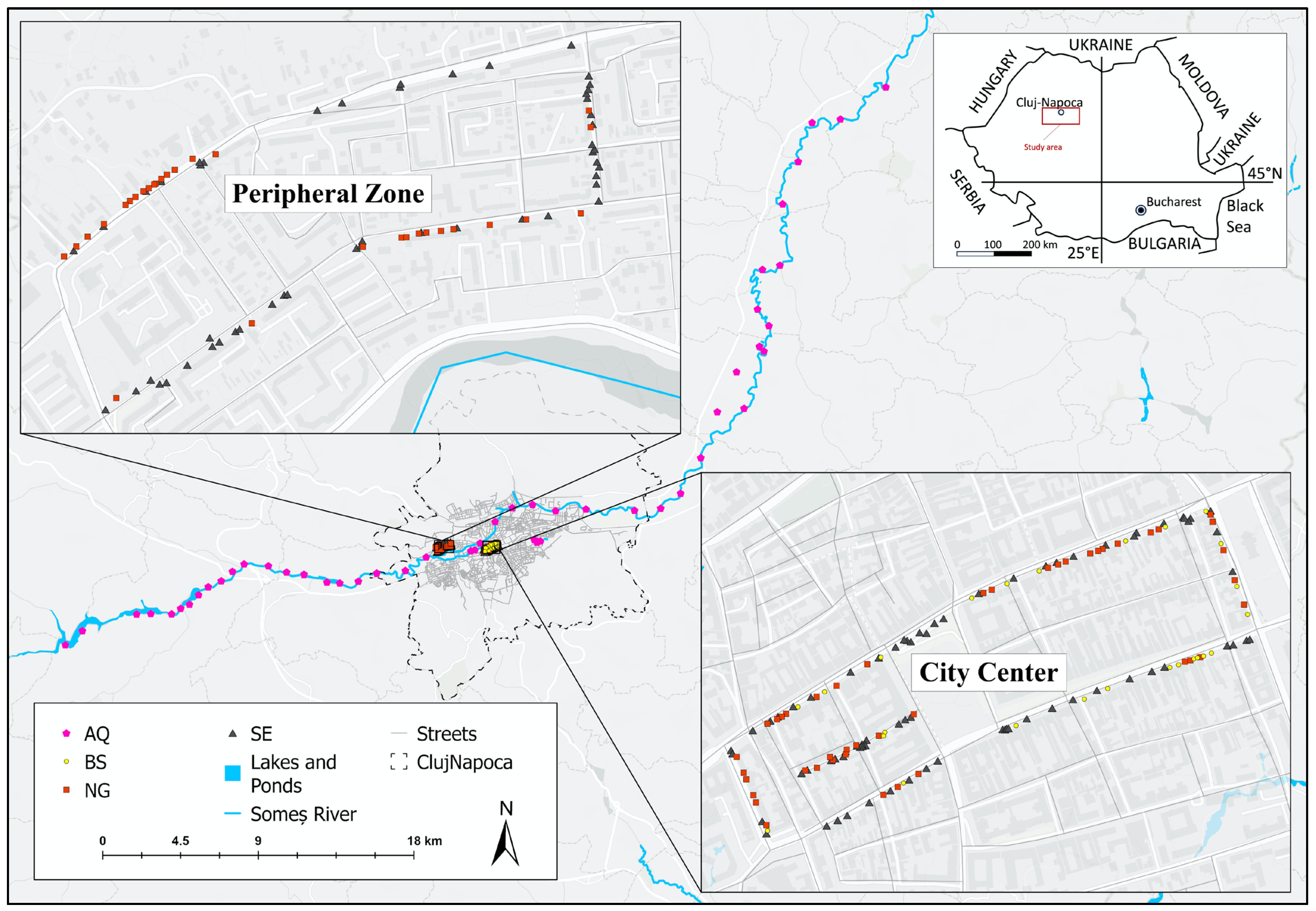
Cluj-Napoca (46°46′ N; 23°35′ E) is a major urban center in northwestern Romania, on the western side of the Transylvanian Depression (Figure 1). The city is the country’s second-largest urban and economic center, with a population of 286,598 inhabitants in 2021 and a total area of 179.2 km2 [63]. It is characterized by mixed residential, commercial, and industrial zones.
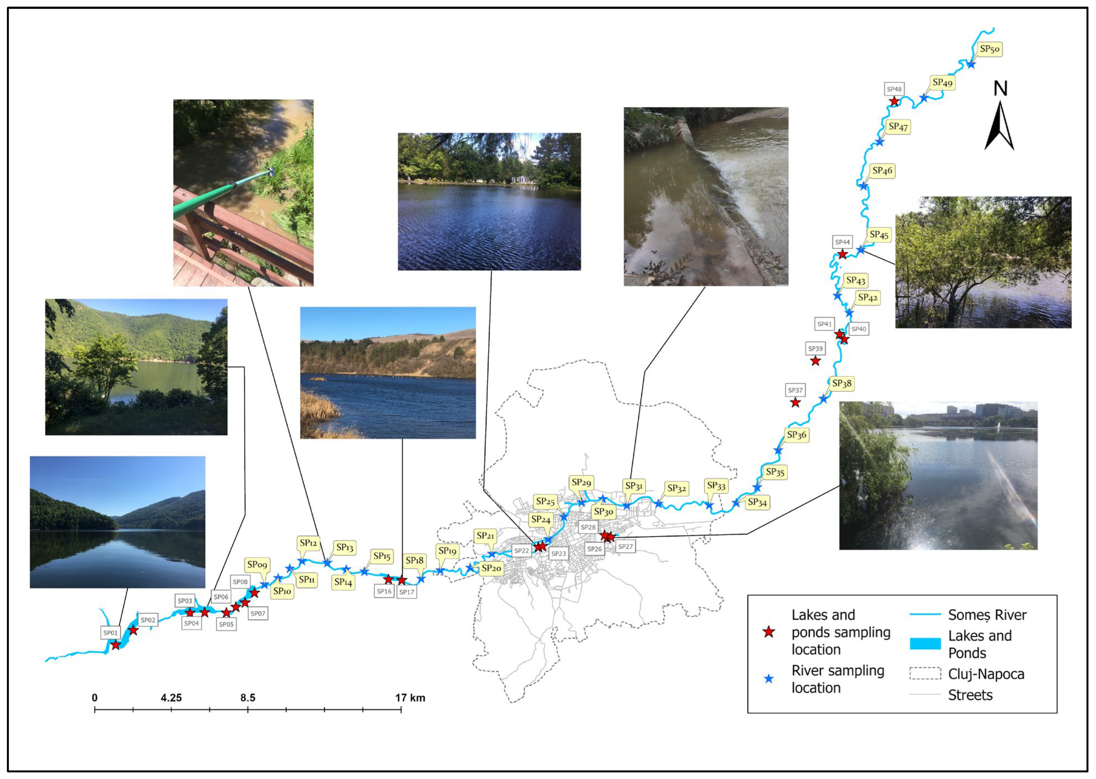
The urban aquatic system (AQ) consists of the Someșul Mic River, which flows west–east through the city, and several urban aquatic features, including two artificial lakes within the metropolitan area—Iulius Mall Lake and Central Park Lake—and Tarnița reservoir, an accumulation lake located upstream of the city (Figure 2). These inland water bodies represent potential sources of methane emissions through biogenic production in sediments and diffusive release at the water–air interface.
Cluj-Napoca provides a representative model for mid-sized Eastern European cities for its diverse energy infrastructure, extensive sewer network, high vehicle density, and variable topography, in addition to ongoing rapid urbanization, all of which contribute to a heterogeneous CH4 emissions landscape.

2.2. Instruments

Two high-sensitivity instruments were employed for trace gas detection:
(i)
The WestSystem package (West Systems SRL, Pontedera, Italy), containing a portable laser spectrometer (Gazomat, Illkirch-Graffenstaden, France) based on Tunable Diode Laser Absorption Spectroscopy (TDLAS), for CH4 detection, with a detection limit of 0.1 ppmv, precision and resolution of 0.1 ppmv, and dynamic range up to 100%, operating at 1 Hz sampling frequency [64].
(ii)
Mira Pico-AERIS (Hayward, CA, USA), based on Mid-Infrared Laser Absorption Spectroscopy (MILAS), for simultaneous detection of CH4 and C2H6. The system measures CH4 over a dynamic range of 10 ppbv to 10,000 ppmv with 1 ppbv precision, and C2H6 over 1 ppbv to 1000 ppmv with 0.5 ppbv precision, both at 1 Hz sampling frequency [65].
The dual-gas detection capability enables the determination of the C2H6/CH4 ratio—a useful diagnostic for differentiating thermogenic from biogenic CH4 sources.

2.3. Instrument Calibration and Quality Assurance/Quality Control (QA/QC)

Calibration and quality assurance/quality control (QA/QC) were applied to ensure the stability, reliability and accuracy of CH4 measurements obtained via TDLAS- and MILAS-based analyzers.
The TDLAS instrument was routinely checked to verify the linearity and response stability under field conditions using a certified reference gas (cylinder code: W_GAS_164_S; 1% CH4 balanced in N2). Periodic checks were performed during measurements to detect potential drift. When performance deviations exceeded acceptable limits, field measurements were suspended, and the instrument was returned to the manufacturer (West Systems SRL, Pontedera, Italy) for factory recalibration.
The MILAS analyzer was similarly evaluated by using a certified reference gas to ensure measurement accuracy. A target gas (CH4: 2487 ppbv) was used to verify the instrument stability during operation. When required, the instrument was returned to the manufacturer (AERIS Technologies, Hayward, CA, USA) for recalibration.
Data quality control procedures included the identification and removal of isolated measurement spikes lacking temporal consistency, which were considered artifacts. This filtering approach was applied particularly to short-duration measurements. A minimum 1 min measuring interval was applied to individual samples to ensure a robust representation of CH4 concentrations.

2.4. Point-Source Measurements

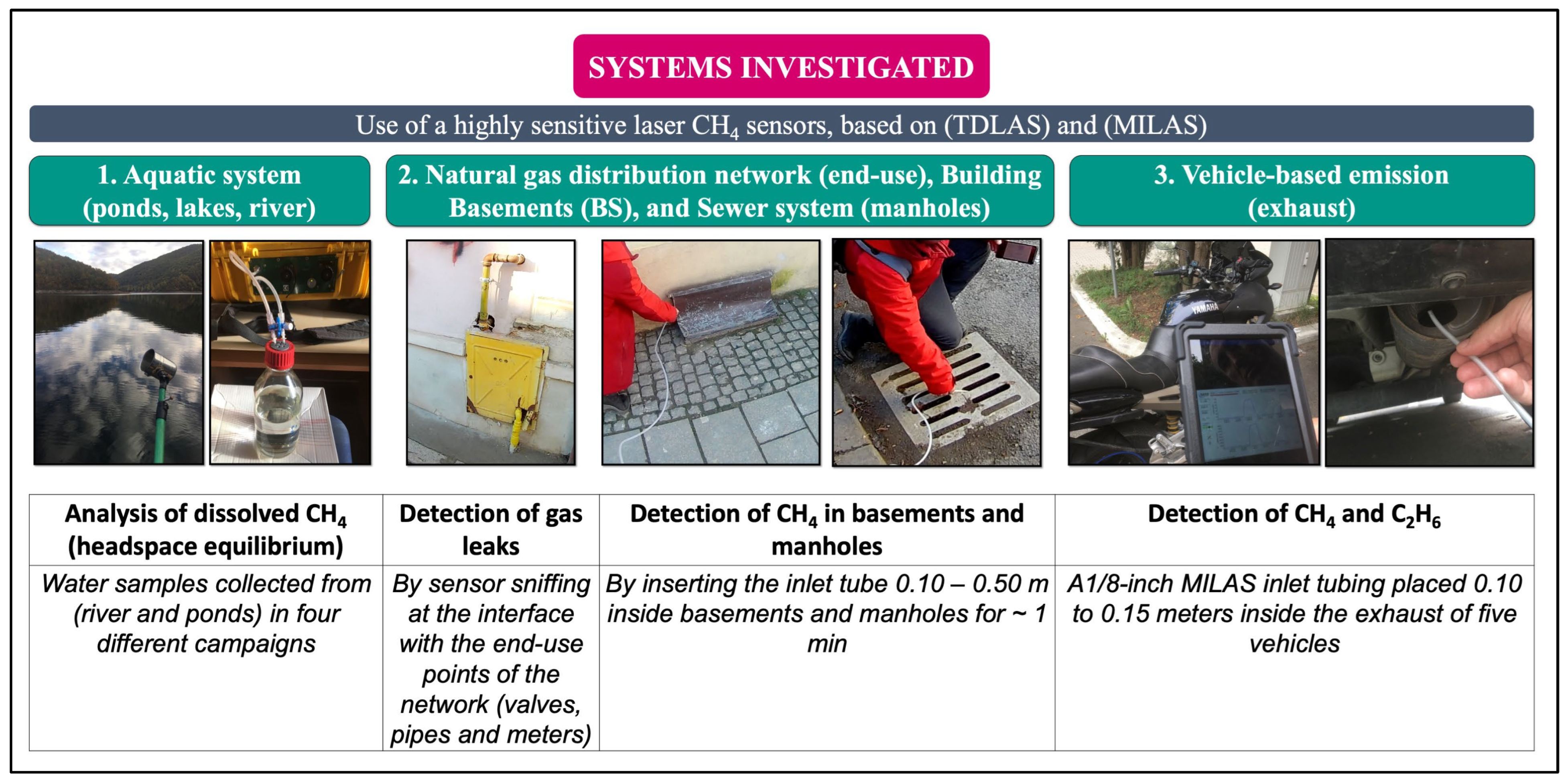
To characterize urban CH4 emissions, point-source measurements were organized into three main investigation levels according to emission environment and sampling strategy (Figure 2):
  • Aquatic System (AQ): Dissolved methane (dCH4) sampling across the river, lakes, and ponds;
  • Urban infrastructure (NG, SE, BSs): Natural gas end-use points, sewer manholes, and building basements, measured in two urban zones differing in land-use intensity;
  • Traffic-based emissions (TEs): CH4 and C2H6 measurements from vehicle exhausts and near-road environments with varying traffic density.
This classification allowed for systematic comparison across diverse urban functions and micro-environments, integrating multiple CH4 sources within a unified observational framework. The background CH4 concentration was determined on previous continuous stationary measurements conducted in Cluj-Napoca, which reported an average value of 2.03 ppmv [62]. In addition, four measurements of CH4 concentrations were performed at street levels outside the urban area in four directions, yielding an average of 2.1 ppmv. Due to the complexity of the urban environments, where multiple overlapping CH4 sources influence atmospheric concentrations, background levels within the city were observed to vary between 2.0 and 2.1 ppmv using the TDLAS analyzer. Based on these observations, the leak indication threshold (LI > 2.2 ppmv; approximately 0.1 ppmv above the observed urban background variability) was adopted to distinguish close-to-source methane enhancements from ambient urban background concentrations.

2.4.1. The Aquatic System (AQ)

Sampling Design
Methane concentration in the dissolved phase (dCH4) from Cluj-Napoca’s urban aquatic system, encompassing the Someșul Mic River (SMR) and several artificial lakes and ponds, was measured (Figure 3). The SMR traverses the city over ~22 km (east–west) and is formed by the confluence of the Someșul Rece River (49 km long) and Someșul Cald River (70 km long) near Gilău.
Two major artificial ponds within the city—Central Park Lake (~12,000 m2) and Iulius Mall Lake (~53,000 m2)—were sampled. To assess potential urban influences, the sampling campaign was extended both upstream and downstream of the city. Four upstream reservoirs formed by damming the river were also investigated:
  • Tarnița Reservoir (~1,280,000 m2);
  • Someșul Cald Reservoir (~930,000 m2);
  • Gilău Reservoir (~550,000 m2);
  • Florești Reservoir (~240,000 m2).
Downstream sites included the SMR reach east of the city and several artificial ponds. Surface areas of all lakes were estimated using Google Earth imagery (Google, Mountain View, CA, USA, 2025).
In total, 50 sampling points (SPs) were distributed along 77 km transects (Figure 3). To capture seasonal variability, four sampling campaigns were conducted during cold and warm seasons (Table 1), yielding 196 water samples in total. Due to logistical constraints related to field and laboratory work, seasonal samples were collected across different years; therefore, interannual variability may influence the observed patterns.
At each site, a 1 L water sample was collected under calm, non-rainy conditions to minimize surface gas disturbance. The equilibration headspace method [66,67] was applied to determine dCH4.
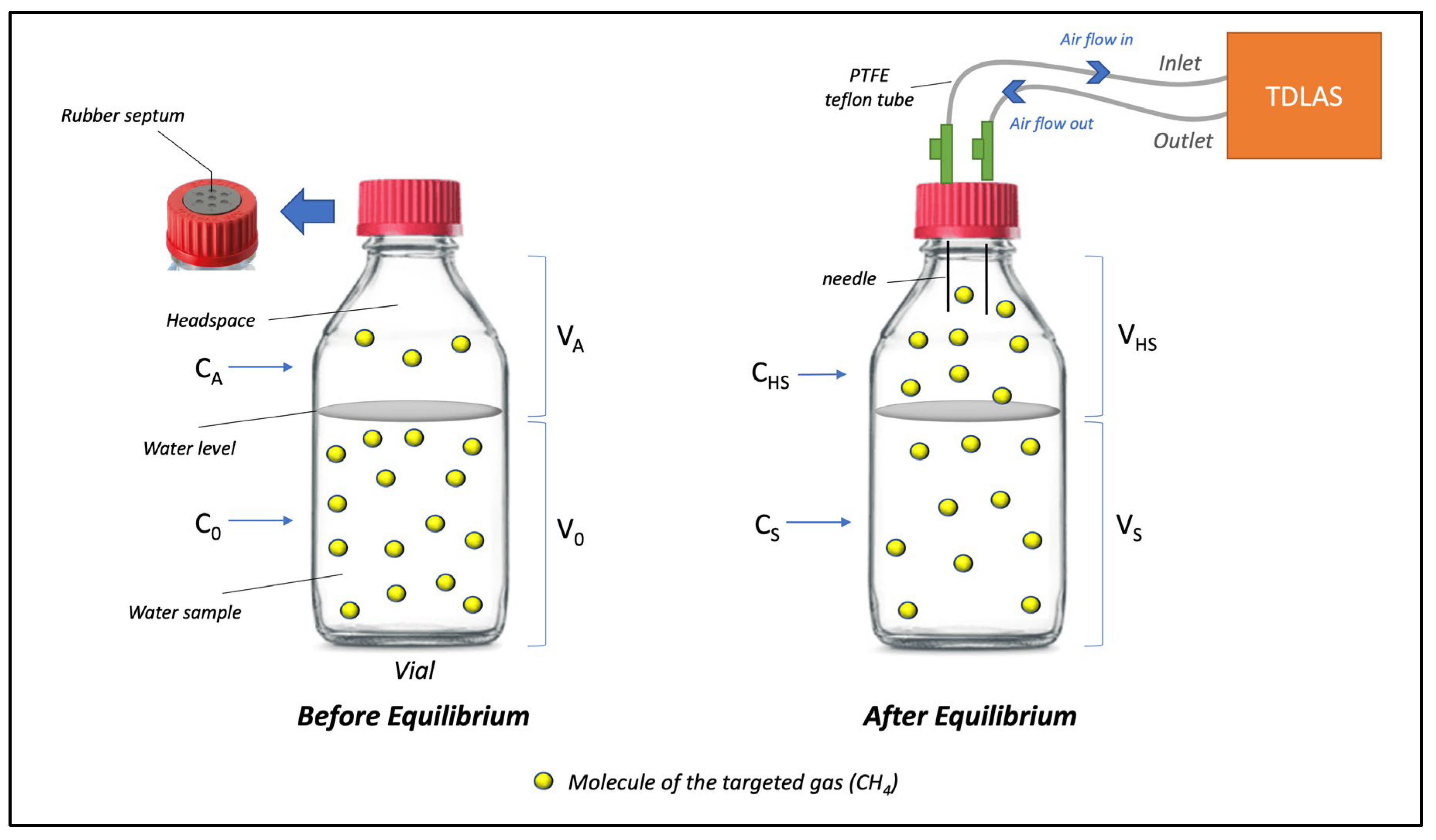
A 700 mL aliquot of the sample was transferred to a 1060 mL DURAN® glass bottle, leaving 360 mL of headspace (headspace-to-liquid ratio ≈ 1:3), optimized for rapid gas equilibration [68]. The bottle was vigorously shaken for 2 min to achieve equilibrium between the liquid and gaseous CH4.
The headspace CH4 concentration was immediately measured using the TDLAS sensor (Gazomat, Illkirch-Graffenstaden, France). Two 1/8-inch Teflon tubes connected to the TDLAS inlet and outlet were inserted through the rubber septum, as illustrated in Figure 4. After each measurement, the instrument was flushed with ambient air until background CH4 levels were re-established, and laboratory ventilation was maintained to prevent gas accumulation.
Calculation of Dissolved CH4
The dissolved CH4 concentrations (C0) were calculated using the Bunsen solubility coefficient [66,69] according to Equation (1):
C 0   =   β · C HS + V H S V s   ( C HS C A )
where: C0 = CH4 concentration in the initial sample before equilibrium; β = Bunsen coefficient, which is 0.035 Lg/Ls for CH4 at 1 atm, 18 °C, salinity 0–10 [66,70]; VHS = headspace volume; VS = sample volume, CHS = measured CH4 concentration in the headspace (ppmv); CA = atmospheric CH4 concentration (ppmv).

2.4.2. Urban Infrastructure Systems

Measurements were conducted in two representative urban zones (Figure 1):
  • City center (CC)—characterized by dense traffic, older buildings, and mixed residential-commercial land use;
  • Peripheral zone (PZ)—dominated by newer infrastructure and lower human activity.
Weather conditions during all surveys (January 2023) were cloudy with temperatures between 2 and 7 °C and wind speeds of 7–11 km h−1 (SW) (meteostat.net). The number of measurement points differed between the CC and PZ for the investigated urban infrastructure systems due to variations in site accessibility and infrastructure density. The CC is characterized by a denser and generally older natural gas distribution network and sewer system, thus providing a higher number of accessible points. In contrast, the PZ is dominated by newer infrastructure with longer distances between manholes of the sewer system and fewer exposed natural gas end-use points. Additionally, several potential measurement points were excluded due to accessibility limitations and safety considerations (e.g., manholes located in the middle of high-traffic streets or restricted access to infrastructure). The measurement approach prioritized spatial representativeness rather than equality in sample size. Consequently, statistical comparisons between the CC and PZ were performed following non-parametric methods such as the Mann–Whitney U-test [71,72].
Natural Gas (NG) End-Use Points
The local natural gas (NG) distribution system supplies residential and commercial consumers through pipelines transporting gas primarily extracted from the Transylvanian Basin, with predominantly microbial origin [73]. Isotopic analysis of a grid sample reported by van Es et al. [62] confirmed the microbial signature of gas (δ13C-CH4 = −64‰, δ2H-CH4 = −180‰).
Measurements targeted accessible end-use components (valves, pipes, and meters) prone to leakage due to corrosion, aging, or mechanical stress. Each point was measured for 60 s at 1 Hz using TDLAS (Figure 2), and coordinates were recorded via Google Maps (Google, Mountain View, CA, USA, 2023).
Sewer System Manholes (SE)
Methane concentrations were measured at 126 manholes distributed between the CC and PZ areas. The number of samples was constrained by accessibility and surface safety conditions. A 1 m long, 1/8-inch Teflon inlet tube was inserted 0.1–0.5 m inside each manhole, and CH4 concentrations were determined in accumulated air for 1 min at 1 Hz (Figure 2).
Building Basement (BS)
Basements were included as a potential yet under-characterized CH4 source. Previous studies by Defratyka et al. [52] reported NG leaks and boiler emissions within basement spaces. In Cluj-Napoca, many old basements are humid, partially buried, and ventilated through street-level windows, providing conditions favorable for methanogenesis and CH4 accumulation.
Measurements were performed at 25 accessible basements (mostly in the CC area) by inserting a 1 m long, 1/8-inch Teflon tube through the window, and the CH4 concentration was measured for 1 min using TDLAS (Figure 2). These measurements were carried out simultaneously with NG and SE surveys.

2.4.3. Traffic-Based Emissions (TEs)

Methane concentrations were measured in two complementary ways:
  • Street-level ambient monitoring with contrasting traffic densities;
  • Direct vehicle exhaust sampling to assess fuel-specific CH4 emissions.
Street-Level Monitoring
Two traffic points were selected:
  • Point 1 (low density-one way road): ~2–3 vehicles min−1;
  • Point 2 (high-density three-street intersection): >30 vehicles min−1.
At both sites, the TDLAS inlet was positioned 1.5 m above ground, facing the roadway to capture vehicle plumes. Video recording was used to document traffic flow and composition, enabling CH4 variability attribution. Weather conditions: 2–7 °C; wind ≈ 9 km hr−1 SW (meteostat.net).
Direct Vehicle Exhaust Sampling
Direct exhaust sampling was performed using the MILAS (Mira Pico) instrument equipped with a 1/8-inch inlet and a ¼-inch inline Zemoner™ filter to prevent soot interference. The inlet was inserted 0.10–0.15 m inside the tailpipe, and CH4 and C2H6 concentrations were recorded at 1 Hz during idling and acceleration phases (Figure 2).
Five in-use vehicles representative of the local traffic fleet were tested, including two diesel-powered passenger vehicles (1.6–2.0 L engines) and three gasoline-powered vehicles, comprising two passenger cars (1.0–1.2 L engines) and one 0.9 L motorcycle. Model years ranged from 2013 to 2024. All vehicles were operated under typical urban driving conditions.
Similar experimental approaches have been employed in previous studies [74,75,76]. Additionally, two exhaust samples were collected for isotopic analysis, as described by van Es et al. [62].

2.5. Statistical Analysis

Statistical analyses were performed to evaluate differences in CH4 concentrations between the CC and PZ. Because the methane concentration data exhibited unequal sample sizes between groups and non-normal distributions (many data points are skewed), non-parametric statistical methods were applied. Differences between the two urban zones were assessed using the Mann–Whitney U-test [71,72]. The Kruskal–Wallis test was used for comparison among multiple categories, followed by Dunn’s post hoc test when significant differences were observed, to identify pairwise differences between groups [77,78]. Statistical analyses were conducted using the scipy.stats library in Python 3.0, and statistical significance was evaluated at a threshold of p < 0.05.

3. Results

Methane concentrations across urban systems in Cluj-Napoca revealed strong spatial and temporal variability. The results are presented in three main categories corresponding to the investigated urban subsystems:
  • The urban aquatic system, focusing on spatial and seasonal patterns of dissolved CH4 (dCH4);
  • Urban infrastructure components, including the natural gas distribution network (NG), the sewer system (SE), and building basements (BSs);
  • Traffic-based emissions (TEs), encompassing both near-road atmospheric CH4 variation and direct exhaust measurements.
This structure allows for systematic comparison among contrasting CH4 source environments, from biogenic aquatic production and sewer methanogenesis to natural gas leaks and thermogenic combustion-derived emissions. The following sections present detailed results for each system, emphasizing spatial heterogeneity, seasonal behavior, and indicative relationships with environmental or infrastructural drivers.

3.1. Urban Aquatic System (AQ)

3.1.1. Seasonal and Spatial Distribution of Dissolved Methane (dCH4)

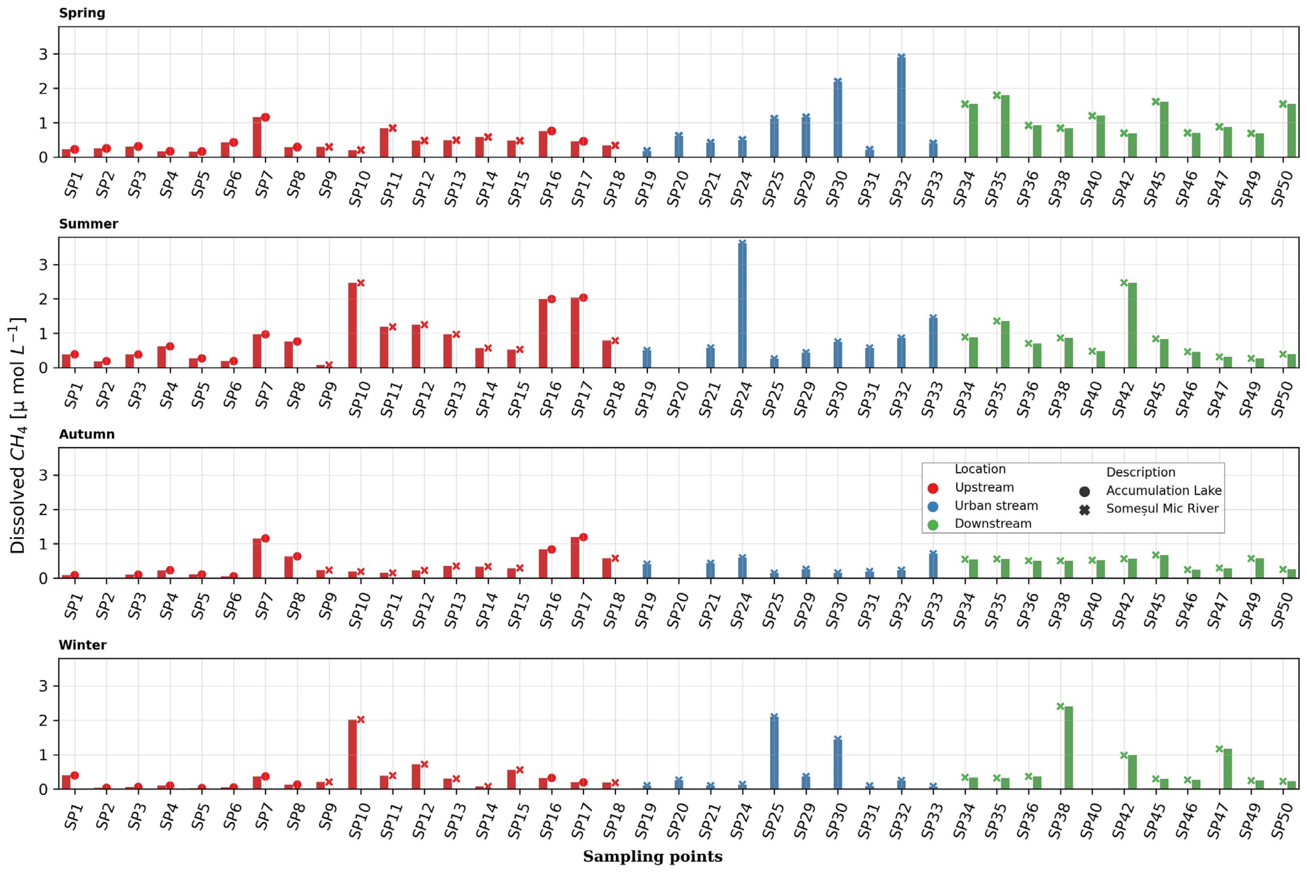
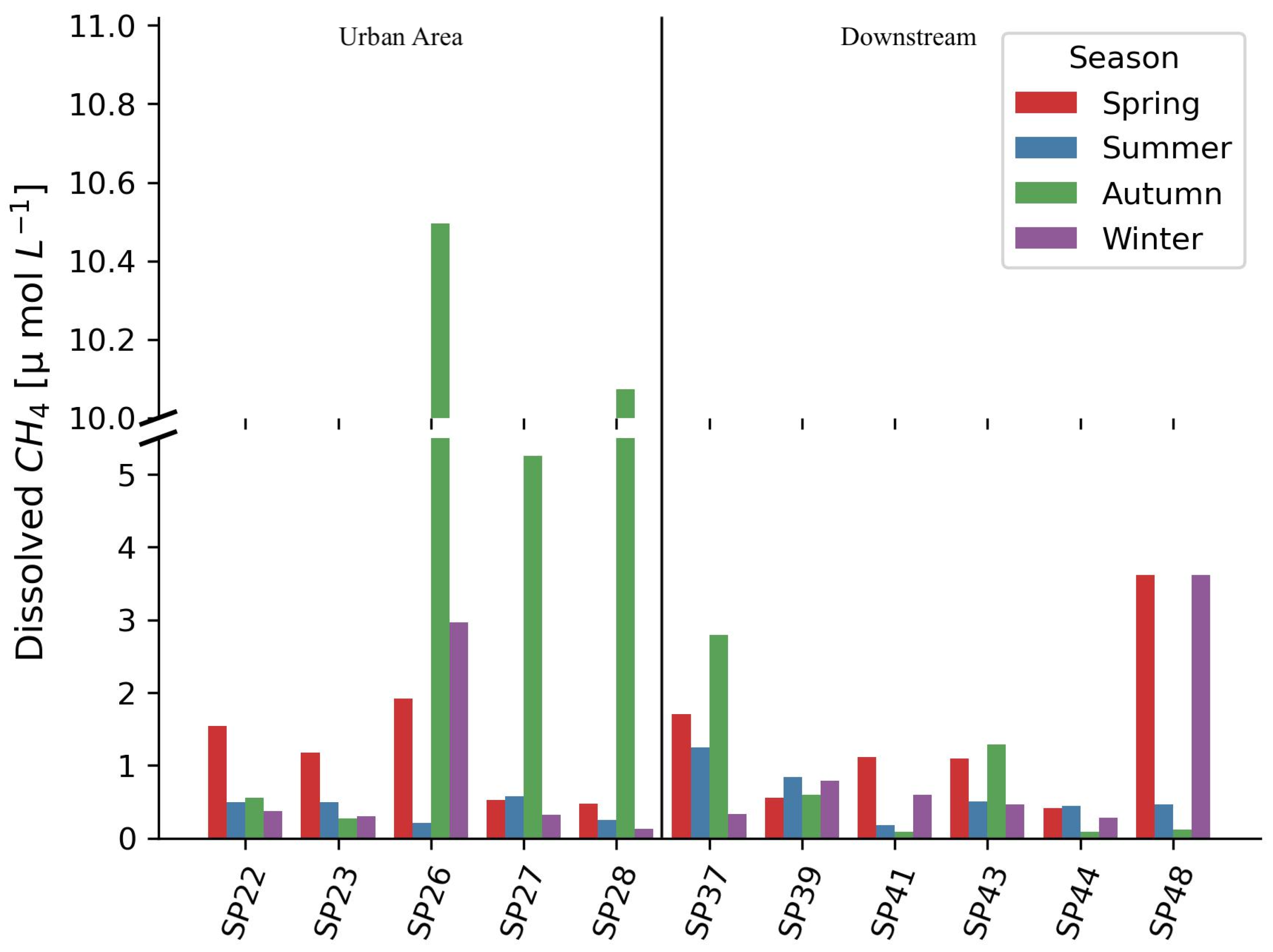
Dissolved methane (dCH4) concentrations displayed a pronounced spatial and temporal variability across the 50 sampling locations spanning Cluj-Napoca’s aquatic system, encompassing accumulation lakes, the river stream, and artificial ponds (Figure 5).
For analytical clarity, the system was divided into two components:
  • The hydrologically connected accumulation lakes and river stream;
  • The isolated artificial ponds.
Across all locations and seasons, dCH4 concentrations were consistently oversaturated relative to atmospheric equilibrium (air-saturated water, ASW = 0.003 µmol L−1), ranging from 0.028 µmol L−1 to 10.495 µmol L−1 (900–300,000% saturation). This pervasive oversaturation indicates persistent in situ CH4 production throughout the aquatic system.
Accumulation Lakes and River
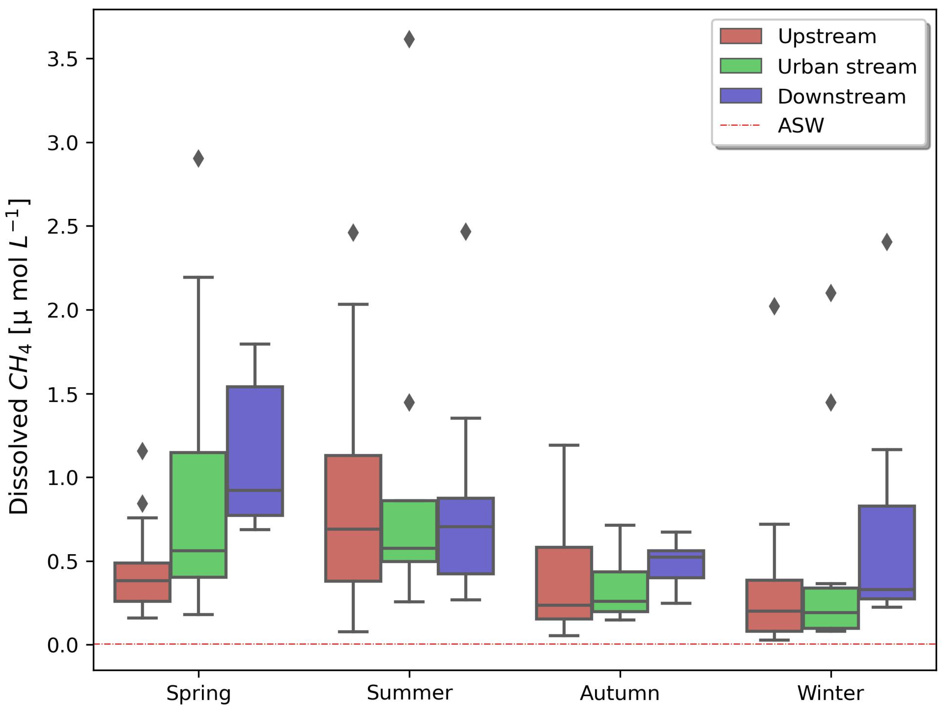
Seasonal patterns of dCH4 (Supplementary Materials, Figure S1) revealed values from 0.028 to 3.615 µmol L−1 (≈900–120,000% saturation), with pronounced elevation during the warmer months. Median dCH4 concentrations were 0.580 µmol L−1 in spring and 0.660 µmol L−1 in summer, decreasing to 0.337 and 0.264 µmol L−1 in autumn and winter, respectively (Table 2, Figure 5). These variations corresponded to a mean seasonal temperature range of −6 to 30 °C (Table 2).
Statistical analysis confirmed significant seasonal differences (Kruskal–Wallis H = 26.359, p < 0.001), with Dunn’s post hoc test showing summer and spring concentrations substantially higher than those in winter and autumn. The strong correlation between dCH4 and temperature supports temperature-dependent microbial methanogenesis during warm periods.
Artificial Ponds
Artificial ponds exhibited a broader concentration range (0.090–10.495 µmol L−1; Table 3), with marked variability between sites and seasons (Figure 6). Median concentration peaks in spring (0.839 µmol L−1) and declines during winter (0.288 µmol L−1), while the highest single dCH4 value (10.495 µmol L−1) occurred in autumn, reflecting localized methane accumulation hotspots.
Despite these trends, seasonal variability was not statistically significant (H = 5.215, p = 0.157), suggesting that site-specific factors, such as organic matter input or sediment oxygen demand, may dominate temperature in controlling CH4 production in these stagnant systems.

3.1.2. Upstream–Urban Stream–Downstream Gradients

Within the connected system, dCH4 concentrations increased progressively from upstream to downstream (Figure 7). The Kruskal–Wallis test confirmed significant spatial variation (H = 14.169, p = 0.0008), with Dunn’s post hoc analysis showing significantly higher downstream concentrations compared to upstream (p < 0.05). No significant differences were observed between urban reach and the other two zones, likely reflecting short-term temporal variability. In artificial ponds, downstream sites also tended to show higher dCH4 than urban ponds but with no statistical significance.
Collectively, these results point to enhanced CH4 accumulation along the hydrological flow, consistent with the integration of both upstream biogenic inputs and local urban contribution. More spatial variations are explained in the land-use influence.

3.1.3. Land-Use Influence on dCH4 Variability

To explore potential land-use drivers, sampling sites were categorized as urban, vegetated, or agricultural, based on CORINE Land Cover data (2018). In the accumulation lakes and river subsystems, dCH4 concentration differed significantly among land-use types (Kruskal–Wallis, H = 7.403, p < 0.05), with urban-adjacent sites exhibiting higher values than vegetated ones (Dunn’s post hoc, p < 0.05). This pattern implies that the urban environment promotes CH4 enrichment, possibly through enhanced organic inputs or reduced oxidation potential.
In the case of artificial ponds, no significant differences have been observed between urban and extra-urban environments (Kruskal–Wallis, H = 1.95, p = 0.38), indicating that the organic matter input and internal biogeochemical conditions may override land-use effects in these more isolated systems.
In summary, across all four seasonal campaigns, the entire aquatic system remained highly supersaturated in dissolved methane, with measured concentrations between 0.028 and 10.495 µmol L−1. Over 85% of samples exceeded 1000% saturation, confirming continuous and spatially heterogeneous CH4 production and transition.
Artificial ponds exhibited the highest absolute concentrations, while accumulation lakes and the river stream displayed clear seasonal and downstream gradients. The positive correlation between dCH4 and temperature, and the elevated concentrations near urban land cover, indicate that urbanization exerts a measurable influence on aquatic CH4 dynamics.
These findings demonstrate that the investigated aquatic system functions as a persistent, spatially structured, and seasonally dynamic CH4 source, reflecting the interplay between natural microbial processes and urban landscape pressures.

3.2. Urban Infrastructure Systems (NG, SE, BSs)

3.2.1. Natural Gas End-Use Points (NG)

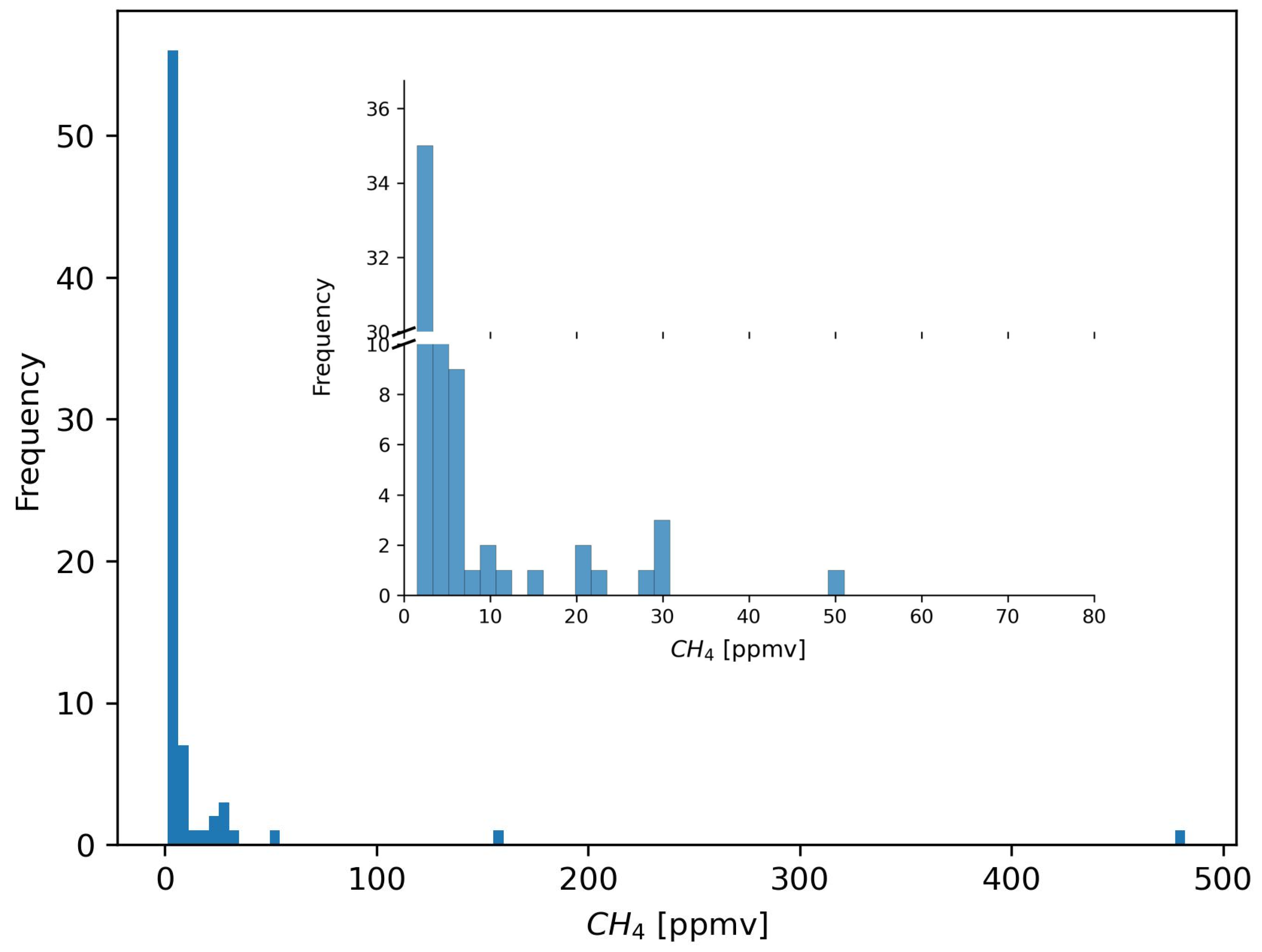
Methane concentrations at 74 natural gas end-use interfaces—valves, joints, and meters—were measured across two urban zones: the city center (CC, n = 44) and the peripheral zone (PZ; n = 30). Concentrations ranged from 1.5 to 482.0 ppmv (mean ± SD = 15.4 ± 60.5 ppmv), showing a highly right-skewed distribution (Figure 8, Table 3).
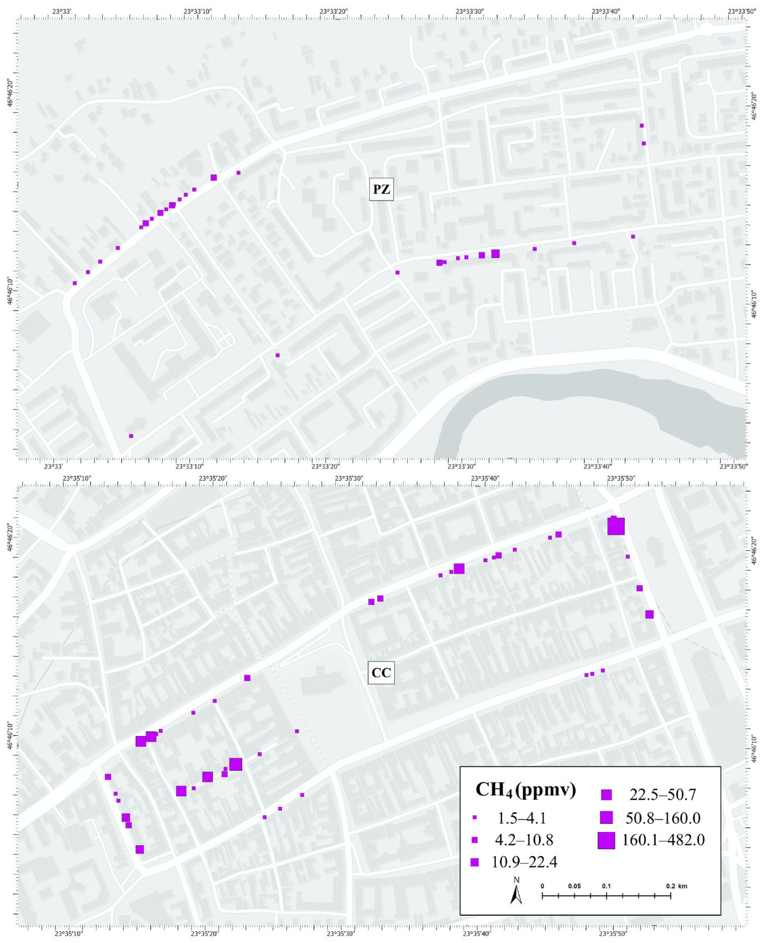
Most observations (≈66%) fell between 1.5 and 2.8 ppmv, within or slightly above average ambient background levels (≈2.2 ppmv). About 24% of measurements ranged between 2.9 and 20.4 ppmv, while 10% exceeded 20.4 ppmv, including several extreme values >400 ppmv. These outliers, largely confined to the CC, disproportionately elevated the mean and indicate localized leakage “hotspots” within the aging central gas distribution network.
Spatial comparison revealed a clear contrast between various urban zones (Mann–Whitney U-test, U = 838.5, p < 0.05), with high CH4 concentrations in the CC (1.5–482.0 ppmv) and low, stable concentrations in the PZ (1.8–15.2 ppmv), reflecting newer infrastructure and fewer leak-prone connections (Figure 9).
From the 74 measured end-use points of the NG distribution network in the city center (CC) and periphery zone (PZ), 60 leak indications (LIs) were identified, accounting for 81% of the total measurement sites. These leaks, characterized by CH4 concentrations exceeding the identified atmospheric background (>2.2 ppmv), are predominantly located in the CC (62%) and PZ (38%). This detection rate is relatively high compared to other urban studies, denoting that the NG network may represent a substantial CH4 emission source.
The right-skewed histogram emphasizes the dominance of low background values punctuated by rare, high-intensity emission events. Such a distribution is characteristic of leak-driven systems, where few sources contribute disproportionately to overall emissions, known as “small-emitters”.

3.2.2. Sewer System (SE) Manholes

Methane concentrations in 126 sewer manholes (CC: n = 75; PZ: n = 51) exhibited a wide range from 1.5 to 1222.0 ppmv, with a mean ± SD of 16.4 ± 109.1 ppmv (Supplementary Materials—Figure S2, Table 3). Zone-specific analysis highlighted marked contrast (Mann–Whitney U-test, U = 2279.5, p < 0.05) for CC [range 1.5–1222.0 ppmv; mean = 25.1 ± 141.1 ppmv; median = 2.2 ppmv] and PZ [range 1.7–35.1 ppmv; mean = 3.7 ± 5.4 ppmv, median = 1.9 ppmv]. The spatial clustering of the elevated values in the CC aligns with denser infrastructure and older sewer systems, which facilitate microbial CH4 emission. In some places, these amounts may be complemented by gas leaking from adjacent pipes of the NG system, confirming the observations of van Es et al. [62].
Of the 126 manholes sampled, 60 showed methane emissions (>2.2 ppmv), with the highest frequency and concentration observed in the city center (CC) compared to the periphery zone (PZ). The mean concentration in the CC (54.6 ppmv) was significantly higher than in the PZ (7.7 ppmv), indicating that certain SE characteristics, such as low slope and higher residence time in the SE system, likely promote greater CH4 accumulation.

3.2.3. Building Basements (BSs)

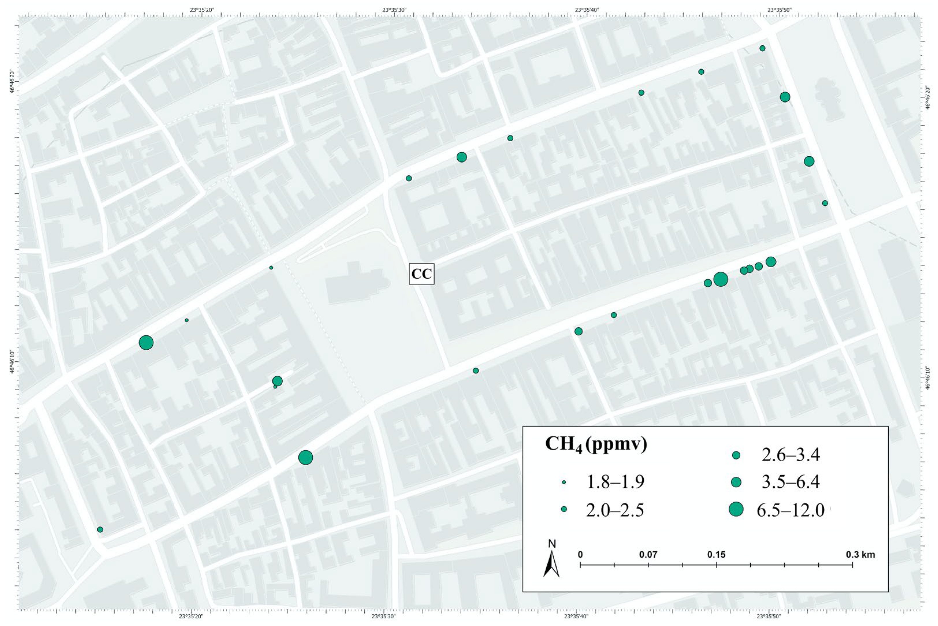
Measurements in 25 building basements across the CC revealed CH4 concentrations from 1.8 to 12.0 ppmv, averaging 3.9 ± 2.7 ppmv (Figure 10, Table 3). Approximately 68% of basements exhibited near-background levels (1.8–4.0 ppmv), while 32% showed elevated methane, up to 12.0 ppmv. Elevated concentrations were mostly observed in abandoned or poorly ventilated basements of older buildings. These confined, humid environments, often containing organic matter, provide good conditions for microbial methanogenesis and potential accumulation zones for diffused NG leaks.
Although data variability limits firm attribution, the observed concentrations and environmental context indicate that basements act as CH4 accumulation micro-environments, representing an under-recognized component of the urban CH4 budget.

3.3. Traffic-Based Emissions (TEs)

3.3.1. Ambient Street-Level Concentrations

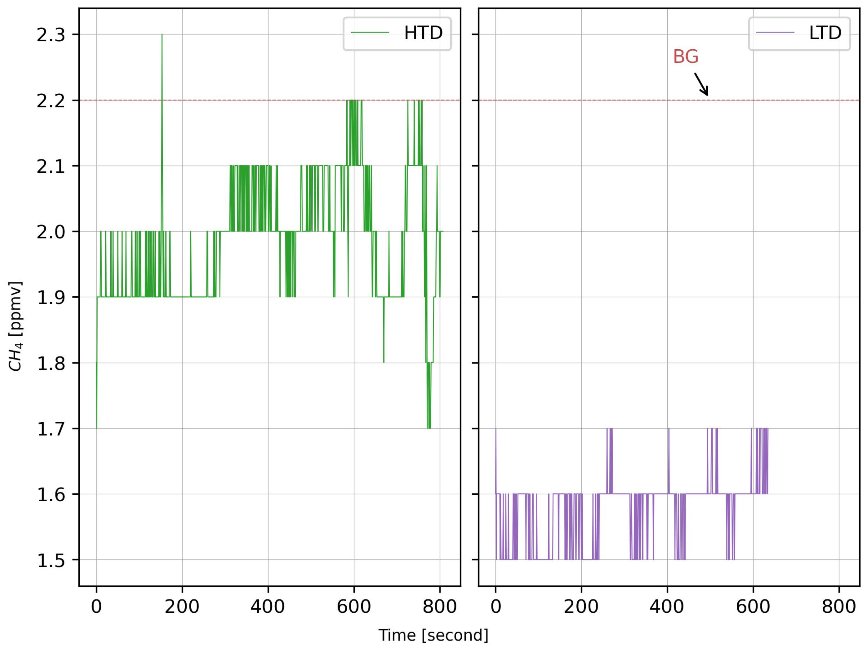
Atmospheric CH4 concentrations measured at two roadside sites in the peripheral zone (PZ) revealed values close to background levels. The high-traffic density (HTD) site averaged 2.0 ± 0.2 ppmv (1.7–2.2 ppmv), whereas the low-traffic density (LTD) site averaged 1.6 ± 0.1 ppmv (1.5–1.7 ppmv) (Figure 11).
Transient CH4 enhancements above baseline coincided with the passage of heavy vehicles (trucks, buses) at the HTD site, as verified by time-synchronized video records. These short-lived peaks were absent at the LTD site, confirming a link between traffic intensity and street-level CH4 fluctuations.
However, due to the absence of isotopic or ethane co-measurements, the attribution of these CH4 plumes specifically to vehicular exhaust remains uncertain, as nearby leaks or wind-driven plumes could also intervene.

3.3.2. Direct Vehicle Exhaust Measurements

Direct exhaust sampling revealed substantial CH4 and C2H6 enrichment relative to ambient air. Across five vehicles of different types, CH4 concentrations reached 162.2 ppmv (mean ± SD = 28.5 ± 37.8 ppmv), as illustrated in Table 3, while C2H6 concentrations peaked at 23,250 ppbv (mean ± SD = 2563 ± 5597 ppbv).
All vehicles exhibited higher emissions during engine acceleration compared to idling, with CH4 and C2H6 increasing simultaneously (Supplementary Materials—Figure S3). The resulting ethane-to-methane C2:C1 ratios ranged between 0.003 and 0.228, reflecting pyrogenic (combustion-related) origins.
One gasoline vehicle (1.2 L engine, 2024 model year) exhibited the highest CH4 (162.2 ppmv) and C2H6 (23,184 ppbv) emissions, followed by the 1 L gasoline-powered vehicle (2018) and 0.9 L motorcycle (2022). Diesel vehicles emitted substantially lower amounts of gas (Figure S3, Table 3).
Vehicle exhaust sampling confirmed that on-road combustion processes emit measurable CH4 with emission intensity modulated by engine characteristics and operation mode. The C2:C1 ratio provides a practical diagnostic for distinguishing vehicle pyrogenic emissions from biogenic or leak-derived CH4 sources in urban atmospheres.

4. Discussion

4.1. Urban Aquatic System (AQ)

4.1.1. Oversaturation and Spatial Patterns

The dissolved methane (dCH4) concentrations in all sampled water bodies were substantially above the air–water saturation level (0.003 μmol L−1), with saturation ranging from 900% to over 3 × 10⁵%. Such oversaturation values have been reported in other urban aquatic systems worldwide, including 6 × 10⁶% in the tropical Krishna River [20], 9 × 10⁵% in the Xiaoyue River in Beijing [79], and 5.6 × 10⁵% in urban ponds in Brussels [18]. Oversaturation of 9.2 × 10⁴% was observed in the Cauvery River (CR), India [80], and in the River Clyde, Scotland [19], and up to 1.8 × 10⁵% in the Yangtze River [81], further confirming that CH4 supersaturation is a pervasive feature of urban aquatic systems globally.
Spatially, rivers exhibited lower dCH4 levels than accumulation lakes, with downstream samples generally enriched compared to upstream sites (Dunn’s post hoc test, p < 0.05), suggesting that downstream segments experience organic loading and local methanogenetic activity, whereas upstream water experiences fast outgassing due to water movement, consistent with the results reported by Leng et al. [81]. In contrast, artificial ponds showed higher concentrations and more limited spatial variability, suggesting persistent CH4 production associated with longer residence time and reduced aquatic turbulence.

4.1.2. Seasonal Dynamics and Temperature

Oversaturation occurred throughout all seasons but peaked in summer, followed by autumn, spring and winter. The positive correlation between dCH4 and temperature indicates that warmer conditions promote microbial activity.
Mean and median dCH4 concentrations during summer and spring were approximately twice those in autumn and winter, consistent with seasonal patterns reported by Wang et al. [82], Tang et al. [83] and Bauduin [18] (Table 4). Elevated summer concentrations are likely promoted by low stream flow, reduced rainfall, and thermal stratification, all of which enhance anaerobic conditions favorable for CH4 production [19].
In colder months, CH4 values persist due to stored gas released from sediments during mechanical disturbance. This suggests that while temperature exerts primary control, diffusion and organic matter availability sustain persistence of oversaturation.

4.1.3. Environmental Drivers and Land-Use Influence

Surrounding land cover had a substantial influence on dCH4 dynamics. Urban areas contributed more efficiently to CH4 oversaturation than vegetated zones, with concentrations reaching up to 120,000% saturation of air–water equilibrium. In contrast, agricultural land showed no significant influence during the four sampling campaigns. This urban effect likely results from runoff carrying organic matter and untreated sewage drained into the water bodies, especially following heavy rainfall events. Patel et al. [20] reported elevated dCH4 concentrations in both treated and untreated sewage, with mean values of 91.82 ± 26.05 μmol L−1 and 37.29 ± 29.52 μmol L−1 respectively, supporting the conclusion that sewage discharge remains a major CH4 source in densely populated urban areas (Table 4).
Similar processes have been observed in other urban areas. Dupuis et al. [84] documented rainfall-driven enrichment in urban lakes in Kalamazoo, MI, USA, while Aguirrezabala-Cámpano et al. [85] reported high CH4 production in Mexico’s La Mancha lagoon in Veracruz, linked to sediment loading and urban runoff.
Multiple environmental drivers may contribute to the observed oversaturation. In colder seasons, CH4 stored in sediment pores may be released slowly through wave-induced disturbance even at reduced temperatures, and fallen autumn leaves represent an input of organic substrates that sustain methanogenesis.

4.1.4. Biochemical Influences

Key biochemical variables—dissolved oxygen (DO), pH, dissolved organic carbon (DOC), and temperature—govern both CH4 production and oxidation. The methanotrophic oxidation in our case may fail to offset rapid CH4 generation under low-DO conditions common in urban waters. However, even if methanotrophs are active, continuous organic inflow and stable stratification sustain CH4 production that exceeds oxidation potentials [20,23,80].

4.1.5. Accumulation Lakes (Hydroelectric Reservoir Influence)

Accumulation lakes, particularly during summer and autumn, showed locally elevated concentrations of dCH4 near the shore (e.g., SP1–SP8, SP16 and SP17). Methane production in accumulation lakes occurs primarily in anoxic bottom sediments, characterized by increased depth and residence time [86,87]. Reis et al. [87] reported methanotrophic removal (<40%) in reservoir mixed layers, implying that vertical stratification controls the balance between production and oxidation, hence highlighting the importance of profiling and sediment sampling in future analyses for fully characterizing CH4 cycling in such systems.

4.1.6. Urban Aquatic System as Methane Hotspots

Collectively, the observed oversaturation, in addition to isotopic signals (δ13C-CH4 = −53.6 to −66.4 ‰; van Es et al. [62]), confirms that Cluj-Napoca’s rivers and ponds act as CH4 hotspots, with emissions dominated by sedimentary biogenic processes, principally acetoclastic methanogenesis. These findings are consistent with global reports that urban aquatic environments represent disproportionally large contributors to atmospheric CH4 relative to their surface area.
Despite clear oversaturation patterns, the quantification of CH4 fluxes and water chemistry is required to provide full insight into emission pathways. Future research on aquatic systems should integrate these data with vertical concentration profiling, isotopic partitioning, and sediment characterization to better constrain the CH4 budget and to identify production and oxidation zones. Additionally, long-term, high-resolution monitoring can also advance our understanding of how hydrological events influence (e.g., floods and droughts) aquatic CH4 dynamics. Such efforts would support integrated mitigation in line with urban climate policies.

4.2. Urban Infrastructure Systems (NG, SE, and BSs)

4.2.1. Natural Gas (NG) End-Use Points

The number of NG measuring points, elevated in the city center (65%) compared to the periphery zone (38%), suggests that NG distribution end-use infrastructure represents a substantial CH4 emission source in the city. This methodological precision ensures robust detection even for small-scale leaks that may be overridden in atmospheric or mobile-based approaches.
Our measurements were conducted directly at potential end-use points (pipes, valves, and meters). This proximity enhances the accuracy of leak identification and effectively reduces uncertainties caused by atmospheric dispersion and dilution, which often affect street-level or mobile measurements (e.g., Lamb et al. [88]). While some uncertainty comes from the absence of definitive source attribution, the closeness and the high concentrations detected can support the robustness of the direct detection approach. Similarly, Xu et al. [89] demonstrated that direct measurements during installation of gas meters at over 1400 NG end-use points in China (residential and commercial units) revealed emissions of 0.008–0.192 kg CH4 per unit, values that could be easily overlooked by atmospheric sampling approaches. Thus, our direct sampling framework provides a strong, quantitative foundation for identifying urban-scale NG leaks. In the USA, Lamb et al. [88] identified substantial emissions from 13 cities, totaling 393 Gg yr−1—far exceeding inventory estimates. Similar trends were observed in Montreal, where Williams et al. [26] reported 451 tons CH4 yr−1, and in multiple Chinese cities, where emission rates scaled with population density [89].
Indirect, mobile-based surveys often underestimate NG-derived CH4 due to atmospheric dilution and source mixing [29,49,90]. Comparatively, European cities show low NG leak frequencies, determined by mobile surveys, in Utrecht and Hamburg [55], in Paris [52], and in Bucharest [59], reflecting improved maintenance and detection practices. These identified leaks in Cluj-Napoca underscore both the vulnerability of old infrastructure and the need for systematic monitoring in rapidly urbanizing regions. Studies combining mobile, aircraft, and stationary approaches, for instance, Lamb et al. [47], have shown that NG leaks account for up to 90% of total urban fluxes, yet these emissions remain systematically underreported in national inventories. The present results confirm that small, distributed leaks at end-use points can collectively constitute a major unaccounted source.
Although detected concentrations in this study remained below the lower explosive limits (LEL; 0.5% CH4), the highest record value of 482 ppmv indicates the potential for localized negative effects, especially in confined or poorly ventilated areas. Hendrick et al. [28] reported that ~15% of urban pipeline leaks in Boston exceeded the LEL, demonstrating that even small leaks can evolve into safety hazards under specific conditions. From a climate perspective, “super-emitter” leaking points may contribute substantially to the total urban CH4 budget, e.g., over 50% [88], implying that targeted detection prioritizing older, high-density urban zones, such as the CC, would substantially achieve both climate and safety co-benefits.

4.2.2. Sewer System (SE) Manholes

The spatial disparity of methane concentrations in the CC compared to PZ reflects the influence of infrastructure density, sewer geometry, and flow dynamics, factors known to regulate anaerobic microenvironments conducive to methanogenesis [91,92,93]. Low slopes and complex network design in the CC likely promote longer hydraulic retention time (HRT) and larger biofilm surface areas, both of which favor microbial CH4 production, with such dynamics mirroring those described for Kolkata [94].
Methane measurements in the sewer system manholes were performed during winter, a period typically associated with reduced microbial activity. Nevertheless, measurable CH4 levels persist, likely sustained by elevated sewage temperatures due to domestic warmwater discharge and by persistent anaerobic biofilms that continue CH4 production under low-flow conditions.
Fries et al. [95] determined 2.1 to 68.8 ppmv across 104 manholes in Cincinnati, Ohio (USA), building on the work of Gallagher et al. [96], who detected approximately 60 ppmv attributed to NG leaks across different U.S. states (Table 4), while Joo et al. [38] reported total SE emissions of 573 tons CH4 yr−1 in Seoul, dominated by microbial processes (C2H6:CH4 < 0.0005). Atmospheric studies in Paris and Bucharest identified sewer-related CH4 contributions of 33% and 63% respectively [52,59], though those lacked direct in situ verifications. Our direct manhole sampling, therefore, provides valuable validation, offering stronger source attribution and confirming that SE systems constitute a significant and underrepresented CH4 source within urban inventories.
Future work should employ long-term, continuous monitoring to capture temporal dynamics, alongside sediment and biofilm analyses to characterize microbial communities and substrate pathways. Incorporating these parameters into predictive models would improve urban CH4 budgets and help identify priority zones for emission reduction.

4.2.3. Building Basements (BSs)

Elevated CH4 levels were predominantly detected in older, poorly ventilated basements. These environments, characterized by high humidity, low oxygen, and organic debris input, provide favorable conditions for both gas accumulation and microbial CH4 production. Isotopic analysis [62] suggested a dual origin for basement CH4, reflecting potential contributions from either NG leaks or biogenic sources, though source attributions remain uncertain.
The contribution of BSs in the urban CH4 budget is not clear, as building basements are still poorly studied sources of CH4 in urban areas. However, while microbial CH4 emissions may decline over time due to ongoing infrastructural and architectural rehabilitation in the CC, including improved sealing at street-level, ventilation and effective drainage of rainwater, the persistent NG leaks remain a major concern. Therefore, further spatial and isotopic investigations are required to reliably distinguish CH4 sources and to apply appropriate mitigation strategies.
Measurements within BSs were limited to 25 samples and were conducted exclusively in the CC due to availability and accessibility constraints. Expanding future surveys to include a larger number of basements across different urban districts would allow for robust assessments of spatial variability and allow for comparisons between old buildings in the CC and newer infrastructure in other parts of the city. Such efforts could help better evaluate the role of building basements and their different environmental conditions, such as ventilation, or proximity to potential NG leaks that might accumulate within the BS environment.
Moreover, the point-source measurements conducted across the three urban infrastructure systems were performed during the winter period, which limits the assessment of the potential temporal variability. Therefore, future direct measurements should incorporate seasonal observations in order to characterize the temporal dynamics of urban CH4 sources.

4.3. Traffic-Based Emissions (TEs)

The short-lived CH4 enhancements observed during the passage of trucks and buses were absent at the low-traffic site, implying a direct influence from vehicle emissions. This was confirmed by direct exhaust concentration measurements at exhaust tailpipes.
Higher C2:C1 ratios during engine acceleration compared to reduced ratios during idling were observed across all vehicles, suggesting that incomplete oxidation during transient engine loads increases both CH4 and C2H6 emissions. Diesel vehicles exhibited relatively low ratios and smaller concentration amplitudes, consistent with more complete combustion and lower unburned hydrocarbons release. In contrast, gasoline vehicles displayed pronounced C2H6-CH4 ratios, indicating less efficient hydrocarbon oxidation.
Several studies have reported contributions of traffic to urban CH4 emissions. For instance, Nakagawa et al. [76] stated that high traffic densities may contribute up to 30% of CH4 urban budget in Nagoya, Japan. Similarly, Venturi et al. [97] attributed up to 14% of Florence’s CH4 to a mix of traffic and domestic heating, while in Bucharest, Fernandez et al. [59] reported 5% of urban atmospheric CH4 originating from pyrogenic sources using a mobile-based approach.
Bezyk et al. [98] referred to the transportation sector as a significant emitter of CH4 via combustion of petroleum products. Chu et al. [75], using sidewalk CH4 measurements coupled with video recording to attribute vehicle types, observed higher CH4 emissions from minibuses but did not identify trucks as major contributors. By contrast, our observations suggest that large vehicles (e.g., trucks) may also be potential contributors. Conversely, Popa et al. [43], using isotopic signature and highway tunnel sampling in Islisberg, Switzerland, reported that traffic is not a significant CH4 contributor.
Isotopic analyses from Cluj-Napoca further support traffic-related CH4 contributions. Air samples collected near traffic areas showed enriched δ13C-CH4 and δ2H signatures (δ13C = −11 ± 4.9‰ and δ2H = −144 ± 5.1 ‰) [62], particularly during winter months, aligning with the findings of Chanton et al. [74] and Nakagawa et al. [76], who attributed δ13CH4-enriched signals (average = −15.4 ± 4.1 ‰; ranging from −3.9 to −22.9‰) to more complete combustion in catalyst-equipped vehicles (Table 4).
In terms of hydrocarbon ratios, our C2:C1 values (0.003–0.228) fall within the typical ranges commonly associated with fossil-fuel-related methane sources. Previous studies have reported similar thresholds for thermogenic or pyrogenic methane, including ratios > 0.01 (Lamb et al. [47]; Fernandez et al. [59]), values between 0.02 and 0.8 (Yacovitch et al. [99]), and ratios exceeding 0.05 (Lowry et al. [16]; Rella et al. [100]). These comparisons support the interpretation that the measured methane enhancements are consistent with fossil-fuel-related CH4 emissions. Furthermore, gasoline-powered vehicles were observed to produce more CH4 and C2H6 than diesel vehicles, corroborating earlier findings by Nam et al. [42] and Chanton et al. [74]. However, lower C2:C1 ratios (~0.003) occasionally occurred during engine idling conditions (Figure S3), indicating variability in combustion efficiency and exhaust composition under different operating modes.
The number of tested vehicles was relatively limited (n = 5), selected to represent commonly used vehicle types in the city, based on engine size and fuel type. Although this subset allowed for an initial assessment of the potential contribution of traffic in urban CH4 emissions, the limited sample size may constrain the representativeness of the results for the entire city vehicle fleet. Consequently, future investigations should include a larger and more diverse set of vehicles, with a broader range of engine technologies, vehicle models, fuel types, and vehicle ages, in order to better characterize methane traffic-related emissions.

4.3.1. Engine Cold Start

The short-term tailpipe measurements were limited to a short duration (<3 min), primarily captured cold-start emissions, and may overrepresent average driving conditions. This also confirms that cold starts produce substantial CH4 spikes. This is consistent with the findings of [101], who observed that the first 3 km of driving after ignition can account for up to 90% of total CH4 emissions. Similar results were reported by Chanton et al. [74], Nam et al. [42] and Nakagawa et al. [76], highlighting how emissions are markedly higher in older vehicles or those lacking catalytic converters.
Consistent with the previous literature, our results showed that gasoline vehicles consistently emitted higher CH4 concentrations than diesel counterparts, with differences exceeding 40 ppmv. This highlights how engine type, fuel composition, and combustion efficiency all influence short-term emission peaks.
Although cold-start events typically occur over a short duration, their contribution to urban CH4 emissions from the transportation sector can be disproportionately large due to inefficient oxidation before the catalytic converter reaches its optimal operating temperature. Urban environments are characterized by frequent short-distance and repeated engine-starting events, such as daily commuting, delivery activities, parking lots, taxi services, and traffic-congested hours. These conditions can generate repeated CH4 spikes.

4.3.2. Broader Implications

These findings indicate that in urban environments like Cluj-Napoca, traffic, especially during cold starts, can represent a non-negligible contributor to elevated CH4 concentrations. Mitigation strategies targeting traffic-related CH4 emissions may include improving catalytic converter efficiency to reduce combustion-related emissions, alongside promoting behavioral and structural changes such as increased cycling, expanded use of public transportation, and the development of walkable urban infrastructure. In this context, local initiatives such as the Park & Ride program and the Green Friday free public transportation campaign implemented by Cluj-Napoca city council represent promising steps toward promoting sustainable mobility and reducing transportation emissions.
As the EU advances its “fit for 55” initiative and targets climate neutrality by 2050 [3,102], reducing traffic CH4 emissions becomes increasingly important. Electrification combined with catalytic installations could significantly reduce cold-start CH4 spikes. Electric vehicle (EV) adoption is already rising, representing 24% of the new vehicle registrations across the EU in 2023 and 90% in Norway [103].
These trends suggest strong potential for long-term CH4 reduction in the transport sector. To support this transition, future studies should integrate extensive temporal measurements and real-time isotopic analysis to better understand the traffic role in urban CH4 inventories. Furthermore, incorporating such findings into city-scale CH4 management strategies may enhance mitigation planning and guide cleaner transportation policies.
Table 4. Summary of reported CH4 concentration ranges (in ppmv) across different urban systems, including urban aquatic system (AQ), natural gas distribution end-use points (NG), sewer system manholes (SE), building basements (BSs), and traffic-related emissions (TEs) from vehicle exhausts.
AQ (µmol L−1)NGSEBSTELocationReference
0.03–185.34Tropical Krishna River Basin (India)Patel et al. [20]
0.39–16.74Two urban ponds in Brussels (Belgium)Bauduin et al. [18]
0.05–12.08Polluted rivers, Chongqing (China)Wang et al. [82]
Up to 27.9Up to 86.1Up to 41.7Paris (France)Defratyka et al. [52]
2.2–10.22.1–13.6Cincinnati, Ohio (USA)Fries et al. [95]
Up to 88.6Washington, DC (USA)Gallagher et al. [96]
Up to 28.6Boston, MA (USA)
Up to 60.0Manhattan, NY (USA)
Up to 54.3Cincinnati, Ohio (USA)
Up to 33.1Durham, NC (USA)
18.0–1068.0Nakagawa et al. [76]
40–100Chanton et al. [74]
0.03–10.501.5–482.01.5–1222.01.8–12.02.1–162.2Cluj-Napoca (Romania)This study
As flux quantification was beyond the scope of the present study, the results do not allow direct estimation of the relative contribution of the investigated urban systems to the overall city-scale CH4 budget. Nevertheless, the concentration measurements provide important insights into the presence and the spatial distribution of potential methane sources within the urban environment. The observed CH4 enhancements across multiple systems highlight the complexity of the urban CH4 emissions and emphasize the importance of system-based investigations for identifying localized emission hotspots. Future studies should therefore focus on quantifying methane fluxes from these urban systems in order to assess their contribution to the total urban methane budget and to support effective mitigation strategies aligned with regional and international climate targets.

5. Conclusions

This study provides the first comprehensive, direct assessment of urban methane (CH4) sources in Cluj-Napoca, Romania, integrating high-resolution field observations across five key urban systems: aquatic system environments (AQs), natural gas distribution end-use points (NG), sewer infrastructure (SE), building basements (BSs), and traffic-based emissions (TEs). The dataset captures spatial heterogeneity and system-specific emission dynamics within a rapidly urbanizing Eastern European context, where systematic CH4 observations remain limited.
A summary overview of the observed methane concentrations highlights the variability across the investigated urban systems. Dissolved CH4 in the AQ showed strong oversaturation relative to the atmospheric equilibrium threshold (2.2 ppmv; equivalent air-saturated water ASW = 0.003 µmol L−1), with measured concentrations ranging from 0.028 to 3.615 µmol L−1. In the urban infrastructure, concentrations determined at NG varied from 1.5 to 482.0 ppmv, while SE measurements showed a wider range between 1.5 and 1222.0 ppmv. Methane concentrations detected in BSs were between 1.8 and 12.0 ppmv, whereas vehicle exhaust measurements reached up to 162.2 ppmv.
Elevated CH4 concentrations were consistently detected across all systems with leak indication threshold (LI > 2.2 ppmv), confirming the widespread presence of both diffuse and localized emission sources. Urban aquatic environments showed strong dissolved CH4 oversaturation—up to 3 × 10⁵% of air–water equilibrium—primarily driven by microbial methanogenesis enhanced by seasonal temperature variability and organic inputs from urban runoff. These findings reinforce the role of inland waters as significant CH4 hotspots in urban landscapes, a component often overlooked in bottom-up emission inventories.
The direct point-source approach has proved to be highly effective for detecting localized NG leaks, reducing uncertainties associated with atmospheric dilution and improving source attribution compared to mobile-only surveys. Similarly, elevated CH4 concentrations in sewer manholes, particularly within the city center, reflected the influence of structural and hydraulic characteristics as key drivers for CH4 variability, highlighting the need to include sewer-related emissions into urban CH4 budgets. Methane accumulation in building basements revealed the possibility of a dual-source contribution—leakage from NG pipelines and in situ microbial production under low-ventilated, moisture-rich conditions—emphasizing an overlooked environmental and safety concern, though source attribution remains uncertain. However, future close-to-source measurements combining CH4 concentrations with isotopic analyses and C2:C1 ratios would help strengthen source attribution and differentiate between thermogenic and microbial methane sources, particularly within the sewer system and basement environments.
Vehicle-related measurements identified short-lived yet distinct CH4 enhancements, with C2:C1 ratios ranging from 0.003 to 0.228, values typically associated with fossil-fuel-related emissions. These concentrations increased markedly during engine acceleration, particularly under “cold-start” conditions, demonstrating that pyrogenic emissions from vehicles can contribute to localized atmospheric CH4 variability in traffic-intense corridors.
Collectively, these findings demonstrate that urban environments function as hybrid methane systems, shaped by anthropogenic and biogenic processes across multiple spatial scales. Integrating direct source measurements with atmospheric inverse modeling offers a powerful framework for refining emission estimates, improving bottom-up inventories, and identifying priority hotspots for mitigation. Embedding such observational evidence into national inventories will enhance emission budgets and support alignment with the EU Green Deal and the Paris Agreement objectives.
Building on previous work in Cluj-Napoca, this study represents a further step in the development of a multi-scale framework for urban methane assessment. Earlier stationary measurements with isotopic analyses provided an integrated city-scale signal and enabled the identification of dominant source sectors, while the street-level walking survey resolved spatial CH4 enhancements and localized hotspots (van Es et al. [62]; Hmoudah & Baciu—under review). The present study complements these approaches through the direct investigation of major urban systems. Together, these three observational scales, stationary, mobile, and point source, provide a coherent and comprehensive characterization of urban methane dynamics, linking atmospheric signals to their emission sources. This integrated framework offers a robust basis for improving urban CH4 inventories and enhances the development of targeted mitigation strategies in complex urban environments.

Supplementary Materials

The following supporting information can be downloaded at https://www.mdpi.com/article/10.3390/atmos17040351/s1: Figure S1: Seasonal distribution of dissolved methane (dCH4) in the urban aquatic system. Figure S2: Methane concentrations (ppmv) measured inside the sewer system in the city center (CC) and periphery zone (PZ) using TDLAS. Figure S3: CH4 and C2H6 concentrations measured in the exhaust of five vehicles (two diesel-powered engines and three gasoline-powered engines).

Author Contributions

M.H., conceptualization, writing—original draft, writing—review and editing, investigation, validation, methodology, software, visualization; C.B., conceptualization, writing—review and editing, supervision, funding acquisition. All authors have read and agreed to the published version of the manuscript.

Funding

This work was supported by the project “Building research and know-how on ENvironmental GAs GEochemistry in Romania (ENGAGE)” funded by the European Union—NextGenerationEU and the Romanian Government, under the National Recovery and Resilience Plan for Romania, contract no. 760039/23 May 2023, code PNRR-C9-I8-CF 14/11 November 2022, through the Romanian Ministry of Research, Innovation and Digitalization, within Component 9, Investment I8.

Institutional Review Board Statement

Not applicable.

Informed Consent Statement

Not applicable.

Data Availability Statement

The data will be made available upon reasonable request.

Acknowledgments

The authors are grateful to the editor and to three anonymous reviewers for their constructive comments and suggestions, which significantly improved the manuscript.

Conflicts of Interest

The authors declare no conflicts of interest.

References

  1. IPCC. Climate Change 2014: Synthesis Report; Contribution of Working Groups I, II and III to the Fifth Assessment Report of the Intergovernmental Panel on Climate Change; Core Writing Team, Pachauri, R.K., Meyer, L.A., Eds.; IPCC: Geneva, Switzerland, 2014. [Google Scholar]
  2. IPCC. Synthesis Report on the IPCC Sixth Assessment Report (AR6); Longer Report; IPCC: Geneva, Switzerland, 2023. [Google Scholar]
  3. European Commission. Joint Research Centre. In GHG Emissions of All World Countries: 2023; European Commission: Luxembourg, 2023. [Google Scholar]
  4. Saunois, M.; Martinez, A.; Poulter, B.; Zhang, Z.; Raymond, P.A.; Regnier, P.; Canadell, J.G.; Jackson, R.B.; Patra, P.K.; Bousquet, P.; et al. Global Methane Budget 2000–2020. Earth Syst. Sci. Data 2025, 17, 1873–1958. [Google Scholar] [CrossRef]
  5. IPCC. Observations: Atmosphere and Surface. In Climate Change 2013: The Physical Science Basis; Contribution of Working Group I to the Fifth Assessment Report of the Intergovernmental Panel on Climate Change; Cambridge University Press: Cambridge, UK; New York, NY, USA, 2013. [Google Scholar]
  6. NOAA. Global Monitoring Laboratory, Carbon Cycle Greenhouse Gases, Trends in CO2, CH4, N2O, SF6; NOAA: Silver Spring, Maryland, 2026.
  7. UNEP; CCAC. Global Methane Emissions: Benefits and Costs of Mitigating Methane Emissions; UNEP: Nairobi, Kenya; CCAC: Paris, France, 2021. [Google Scholar]
  8. Tate, K.R. Soil Methane Oxidation and Land-Use Change–from Process to Mitigation. Soil Biol. Biochem. 2015, 80, 260–272. [Google Scholar] [CrossRef]
  9. Tate, K.R.; Ross, D.J.; Saggar, S.; Hedley, C.B.; Dando, J.; Singh, B.K.; Lambie, S.M. Methane Uptake in Soils from Pinus Radiata Plantations, a Reverting Shrubland and Adjacent Pastures: Effects of Land-Use Change, and Soil Texture, Water and Mineral Nitrogen. Soil. Biol. Biochem. 2007, 39, 1437–1449. [Google Scholar] [CrossRef]
  10. Crippa, M.; Guizzardi, D.; Pisoni, E.; Solazzo, E.; Guion, A.; Muntean, M.; Florczyk, A.; Schiavina, M.; Melchiorri, M.; Hutfilter, A.F. Global Anthropogenic Emissions in Urban Areas: Patterns, Trends, and Challenges. Environ. Res. Lett. 2021, 16, 074033. [Google Scholar] [CrossRef]
  11. UN. DESA World Urbanization Prospects: The 2018 Revision; UN: New York, NY, USA, 2019; ISBN 978-92-1-004314-4. [Google Scholar]
  12. Liu, Y.; Paris, J.-D.; Vrekoussis, M.; Quéhé, P.-Y.; Desservettaz, M.; Kushta, J.; Dubart, F.; Demetriou, D.; Bousquet, P.; Sciare, J. Reconciling a National Methane Emission Inventory with In-Situ Measurements. Sci. Total Environ. 2023, 901, 165896. [Google Scholar] [CrossRef]
  13. Vogel, F.; Ars, S.; Wunch, D.; Lavoie, J.; Gillespie, L.; Maazallahi, H.; Röckmann, T.; Nęcki, J.; Bartyzel, J.; Jagoda, P.; et al. Ground-Based Mobile Measurements to Track Urban Methane Emissions from Natural Gas in 12 Cities across Eight Countries. Environ. Sci. Technol. 2024, 58, 2271–2281. [Google Scholar] [CrossRef]
  14. Zazzeri, G.; Graven, H.; Xu, X.; Saboya, E.; Blyth, L.; Manning, A.J.; Chawner, H.; Wu, D.; Hammer, S. Radiocarbon Measurements Reveal Underestimated Fossil CH4 and CO2 Emissions in London. Geophys. Res. Lett. 2023, 50, e2023GL103834. [Google Scholar] [CrossRef]
  15. Liang, L.; Lal, R.; Du, Z.; Wu, W.; Meng, F. Estimation of Nitrous Oxide and Methane Emission from Livestock of Urban Agriculture in Beijing. Agric. Ecosyst. Environ. 2013, 170, 28–35. [Google Scholar] [CrossRef]
  16. Lowry, D.; Fisher, R.E.; France, J.L.; Coleman, M.; Lanoisellé, M.; Zazzeri, G.; Nisbet, E.G.; Shaw, J.T.; Allen, G.; Pitt, J.; et al. Environmental Baseline Monitoring for Shale Gas Development in the UK: Identification and Geochemical Characterisation of Local Source Emissions of Methane to Atmosphere. Sci. Total Environ. 2020, 708, 134600. [Google Scholar] [CrossRef]
  17. Röckmann, T.; Eyer, S.; Van Der Veen, C.; Popa, M.E.; Tuzson, B.; Monteil, G.; Houweling, S.; Harris, E.; Brunner, D.; Fischer, H.; et al. In Situ Observations of the Isotopic Composition of Methane at the Cabauwtall Tower Site. Atmos. Chem. Phys. 2016, 16, 10469–10487. [Google Scholar] [CrossRef]
  18. Bauduin, T.; Gypens, N.; Borges, A.V. Sub-Daily Variability of Carbon Dioxide, Methane, and Nitrous Oxide Emissions from Two Urban Ponds in Brussels (Belgium). J. Environ. Manag. 2025, 373, 123627. [Google Scholar] [CrossRef] [PubMed]
  19. Brown, A.M.; Bass, A.M.; Skiba, U.; MacDonald, J.M.; Pickard, A.E. Urban Landscapes and Legacy Industry Provide Hotspots for Riverine Greenhouse Gases: A Source-to-Sea Study of the River Clyde. Water Res. 2023, 236, 119969. [Google Scholar] [CrossRef]
  20. Patel, L.; Singh, R.; Thottathil, S.D. Land Use Drivers of Riverine Methane Dynamics in a Tropical River Basin, India. Water Res. 2023, 228, 119380. [Google Scholar] [CrossRef]
  21. Qing, X.; Qi, B.; Lin, Y.; Chen, Y.; Zang, K.; Liu, S.; Ma, Q.; Qiu, S.; Jiang, K.; Xiong, H.; et al. Characteristics of the Methane (CH4) Mole Fraction in a Typical City and Suburban Site in the Yangtze River Delta, China. Atmos. Pollut. Res. 2022, 13, 101498. [Google Scholar] [CrossRef]
  22. Zhang, W.; Li, H.; Xiao, Q.; Li, X. Urban Rivers Are Hotspots of Riverine Greenhouse Gas (N2O, CH4, CO2) Emissions in the Mixed-Landscape Chaohu Lake Basin. Water Res. 2021, 189, 116624. [Google Scholar] [CrossRef] [PubMed]
  23. Zhao, G.; Wang, D.; Sun, T.; Ding, Y.; Chen, S.; Li, Y.; Sun, H.; Wu, C.; Yu, Z.; Chen, Z. Emission of Greenhouse Gas from Urban Polluted River during Different Rainfall Events: Typhoon and Storm Will Promote Stronger Evasions. J. Hydrol. 2023, 625, 130166. [Google Scholar] [CrossRef]
  24. Duren, R.M.; Thorpe, A.K.; Foster, K.T.; Rafiq, T.; Hopkins, F.M.; Yadav, V.; Bue, B.D.; Thompson, D.R.; Conley, S.; Colombi, N.K.; et al. California’s Methane Super-Emitters. Nature 2019, 575, 180–184. [Google Scholar] [CrossRef]
  25. García, M.Á.; Sánchez, M.L.; Pérez, I.A.; Ozores, M.I.; Pardo, N. Influence of Atmospheric Stability and Transport on CH4 Concentrations in Northern Spain. Sci. Total Environ. 2016, 550, 157–166. [Google Scholar] [CrossRef]
  26. Williams, J.P.; Ars, S.; Vogel, F.; Regehr, A.; Kang, M. Differentiating and Mitigating Methane Emissions from Fugitive Leaks from Natural Gas Distribution, Historic Landfills, and Manholes in Montréal, Canada. Environ. Sci. Technol. 2022, 56, 16686–16694. [Google Scholar] [CrossRef]
  27. Xueref-Remy, I.; Zazzeri, G.; Bréon, F.M.; Vogel, F.; Ciais, P.; Lowry, D.; Nisbet, E.G. Anthropogenic Methane Plume Detection from Point Sources in the Paris Megacity Area and Characterization of Their δ13C Signature. Atmos. Environ. 2020, 222, 117055. [Google Scholar] [CrossRef]
  28. Hendrick, M.F.; Ackley, R.; Sanaie-Movahed, B.; Tang, X.; Phillips, N.G. Fugitive Methane Emissions from Leak-Prone Natural Gas Distribution Infrastructure in Urban Environments. Environ. Pollut. 2016, 213, 710–716. [Google Scholar] [CrossRef]
  29. Jackson, R.B.; Down, A.; Phillips, N.G.; Ackley, R.C.; Cook, C.W.; Plata, D.L.; Zhao, K. Natural Gas Pipeline Leaks Across Washington, DC. Environ. Sci. Technol. 2014, 48, 2051–2058. [Google Scholar] [CrossRef] [PubMed]
  30. McKain, K.; Down, A.; Raciti, S.M.; Budney, J.; Hutyra, L.R.; Floerchinger, C.; Herndon, S.C.; Nehrkorn, T.; Zahniser, M.S.; Jackson, R.B.; et al. Methane Emissions from Natural Gas Infrastructure and Use in the Urban Region of Boston, Massachusetts. Proc. Natl. Acad. Sci. USA 2015, 112, 1941–1946. [Google Scholar] [CrossRef] [PubMed]
  31. Foster, C.S.; Crosman, E.T.; Holland, L.; Mallia, D.V.; Fasoli, B.; Bares, R.; Horel, J.; Lin, J.C. Confirmation of Elevated Methane Emissions in Utah’s Uintah Basin With Ground-Based Observations and a High-Resolution Transport Model. J. Geophys. Res. Atmos. 2017, 122, 13026–13044. [Google Scholar] [CrossRef]
  32. Heimburger, A.M.F.; Harvey, R.M.; Shepson, P.B.; Stirm, B.H.; Gore, C.; Turnbull, J.; Cambaliza, M.O.L.; Salmon, O.E.; Kerlo, A.-E.M.; Lavoie, T.N.; et al. Assessing the Optimized Precision of the Aircraft Mass Balance Method for Measurement of Urban Greenhouse Gas Emission Rates through Averaging. Elem. Sci. Anthr. 2017, 5, 26. [Google Scholar] [CrossRef]
  33. Yang, S.; Lan, X.; Talbot, R.; Liu, L. Characterizing Anthropogenic Methane Sources in the Houston and Barnett Shale Areas of Texas Using the Isotopic Signature δ13C in CH4. Sci. Total Environ. 2019, 696, 133856. [Google Scholar] [CrossRef]
  34. Chen, H.; Ye, J.; Zhou, Y.; Wang, Z.; Jia, Q.; Nie, Y.; Li, L.; Liu, H.; Benoit, G. Variations in CH4 and CO2 Productions and Emissions Driven by Pollution Sources in Municipal Sewers: An Assessment of the Role of Dissolved Organic Matter Components and Microbiota. Environ. Pollut. 2020, 263, 114489. [Google Scholar] [CrossRef]
  35. Chen, Y.; Wu, J.; Zhao, J.; Yang, H.; Attaran Dovom, H.; Sivakumar, M.; Jiang, G. A Critical Review of Sulfide and Methane Control in Urban Sewer Systems Using Nitrogen Compounds. Water Res. 2025, 277, 123314. [Google Scholar] [CrossRef]
  36. Daelman, M.R.J.; van Voorthuizen, E.M.; van Dongen, U.G.J.M.; Volcke, E.I.P.; van Loosdrecht, M.C.M. Methane Emission during Municipal Wastewater Treatment. Water Res. 2012, 46, 3657–3670. [Google Scholar] [CrossRef]
  37. Eijo-Río, E.; Petit-Boix, A.; Villalba, G.; Suárez-Ojeda, M.E.; Marin, D.; Amores, M.J.; Aldea, X.; Rieradevall, J.; Gabarrell, X. Municipal Sewer Networks as Sources of Nitrous Oxide, Methane and Hydrogen Sulphide Emissions: A Review and Case Studies. J. Environ. Chem. Eng. 2015, 3, 2084–2094. [Google Scholar] [CrossRef]
  38. Joo, J.; Jeong, S.; Shin, J.; Chang, D.Y. Missing Methane Emissions from Urban Sewer Networks. Environ. Pollut. 2023, 342, 123101. [Google Scholar] [CrossRef] [PubMed]
  39. Zhao, X.; Jin, X.K.; Guo, W.; Zhang, C.; Shan, Y.L.; Du, M.X.; Tillotson, M.R.; Yang, H.; Liao, X.W.; Li, Y.P. China’s Urban Methane Emissions from Municipal Wastewater Treatment Plant. Earth’s Future 2019, 7, 480–490. [Google Scholar] [CrossRef]
  40. Pan, D.; Tao, L.; Sun, K.; Golston, L.M.; Miller, D.J.; Zhu, T.; Qin, Y.; Zhang, Y.; Mauzerall, D.L.; Zondlo, M.A. Methane Emissions from Natural Gas Vehicles in China. Nat. Commun. 2020, 11, 4588. [Google Scholar] [CrossRef] [PubMed]
  41. Hu, N.; Liu, S.; Gao, Y.; Xu, J.; Zhang, X.; Zhang, Z.; Lee, X. Large Methane Emissions from Natural Gas Vehicles in Chinese Cities. Atmos. Environ. 2018, 187, 374–380. [Google Scholar] [CrossRef]
  42. Nam, E.K.; Jensen, T.E.; Wallington, T.J. Methane Emissions from Vehicles. Environ. Sci. Technol. 2004, 38, 2005–2010. [Google Scholar] [CrossRef] [PubMed]
  43. Popa, M.E.; Vollmer, M.K.; Jordan, A.; Brand, W.A.; Pathirana, S.L.; Rothe, M.; Röckmann, T. Vehicle Emissions of Greenhouse Gases and Related Tracers from a Tunnel Study: CO:CO2, N2O:CO2, CH4:CO2, O2:CO2 Ratios, and the Stable Isotopes 13C and 18O in CO2 and CO. Atmos. Chem. Phys. 2014, 14, 2105–2123. [Google Scholar] [CrossRef]
  44. Atherton, E.; Risk, D.; Fougère, C.; Lavoie, M.; Marshall, A.; Werring, J.; Williams, J.P.; Minions, C. Mobile Measurement of Methane Emissions from Natural Gas Developments in Northeastern British Columbia, Canada. Atmos. Chem. Phys. 2017, 17, 12405–12420. [Google Scholar] [CrossRef]
  45. Cambaliza, M.O.L.; Shepson, P.B.; Bogner, J.; Caulton, D.R.; Stirm, B.; Sweeney, C.; Montzka, S.A.; Gurney, K.R.; Spokas, K.; Salmon, O.E.; et al. Quantification and Source Apportionment of the Methane Emission Flux from the City of Indianapolis. Elem. Sci. Anthr. 2015, 3, 000037. [Google Scholar] [CrossRef]
  46. Hugenholtz, C.H.; Vollrath, C.; Gough, T.; Wearmouth, C.; Fox, T.; Barchyn, T.; Billinghurst, C. Methane Emissions from Above-Ground Natural Gas Distribution Facilities in the Urban Environment: A Fence Line Methodology and Case Study in Calgary, Alberta, Canada. J. Air Waste Manag. Assoc. 2021, 71, 1319–1332. [Google Scholar] [CrossRef]
  47. Lamb, B.K.; Cambaliza, M.O.L.; Davis, K.J.; Edburg, S.L.; Ferrara, T.W.; Floerchinger, C.; Heimburger, A.M.F.; Herndon, S.; Lauvaux, T.; Lavoie, T.; et al. Direct and Indirect Measurements and Modeling of Methane Emissions in Indianapolis, Indiana. Environ. Sci. Technol. 2016, 50, 8910–8917. [Google Scholar] [CrossRef]
  48. Mays, K.L.; Shepson, P.B.; Stirm, B.H.; Karion, A.; Sweeney, C.; Gurney, K.R. Aircraft-Based Measurements of the Carbon Footprint of Indianapolis. Environ. Sci. Technol. 2009, 43, 7816–7823. [Google Scholar] [CrossRef] [PubMed]
  49. Phillips, N.G.; Ackley, R.; Crosson, E.R.; Down, A.; Hutyra, L.R.; Brondfield, M.; Karr, J.D.; Zhao, K.; Jackson, R.B. Mapping Urban Pipeline Leaks: Methane Leaks across Boston. Environ. Pollut. 2013, 173, 1–4. [Google Scholar] [CrossRef]
  50. Pitt, J.R.; Lopez-Coto, I.; Karion, A.; Hajny, K.D.; Tomlin, J.; Kaeser, R.; Jayarathne, T.; Stirm, B.H.; Floerchinger, C.R.; Loughner, C.P.; et al. Underestimation of Thermogenic Methane Emissions in New York City. Environ. Sci. Technol. 2024, 58, 9147–9157. [Google Scholar] [CrossRef]
  51. Weichenthal, S.; Van Rijswijk, D.; Kulka, R.; You, H.; Van Ryswyk, K.; Willey, J.; Dugandzic, R.; Sutcliffe, R.; Moulton, J.; Baike, M.; et al. The Impact of a Landfill Fire on Ambient Air Quality in the North: A Case Study in Iqaluit, Canada. Environ. Res. 2015, 142, 46–50. [Google Scholar] [CrossRef]
  52. Defratyka, S.M.; Paris, J.-D.; Yver-Kwok, C.; Fernandez, J.M.; Korben, P.; Bousquet, P. Mapping Urban Methane Sources in Paris, France. Environ. Sci. Technol. 2021, 55, 8583–8591. [Google Scholar] [CrossRef]
  53. Gioli, B.; Toscano, P.; Lugato, E.; Matese, A.; Miglietta, F.; Zaldei, A.; Vaccari, F.P. Methane and Carbon Dioxide Fluxes and Source Partitioning in Urban Areas: The Case Study of Florence, Italy. Environ. Pollut. 2012, 164, 125–131. [Google Scholar] [CrossRef] [PubMed]
  54. Helfter, C.; Tremper, A.H.; Halios, C.H.; Kotthaus, S.; Bjorkegren, A.; Grimmond, C.S.B.; Barlow, J.F.; Nemitz, E. Spatial and Temporal Variability of Urban Fluxes of Methane, Carbon Monoxideand Carbon Dioxide above London, UK. Atmos. Chem. Phys. 2016, 16, 10543–10557. [Google Scholar] [CrossRef]
  55. Maazallahi, H.; Fernandez, J.M.; Menoud, M.; Zavala-Araiza, D.; Weller, Z.D.; Schwietzke, S.; von Fischer, J.C.; Denier van der Gon, H.; Röckmann, T. Methane Mapping, Emission Quantification, and Attribution in Two European Cities: Utrecht (NL) and Hamburg (DE). Atmos. Chem. Phys. 2020, 20, 14717–14740. [Google Scholar] [CrossRef]
  56. Ricci, A.; Cremonini, S.; Severi, P.; Tassi, F.; Vaselli, O.; Rizzo, A.L.; Caracausi, A.; Grassa, F.; Fiebig, J.; Capaccioni, B. Sources and Migration Pathways of Methane and Light Hydrocarbons in the Subsurface of the Southern Po River Basin (Northern Italy). Mar. Pet. Geol. 2023, 147, 105981. [Google Scholar] [CrossRef]
  57. Shorter, J.H.; Mcmanus, J.B.; Kolb, C.E.; Allwine, E.J.; Lamb, B.K.; Mosher, B.W.; Harriss, R.C.; Partchatka, U.; Fischer, H.; Harris, G.W.; et al. Methane Emission Measurements in Urban Areas in Eastern Germany. J. Atmos. Chem. 1996, 24, 121–140. [Google Scholar] [CrossRef]
  58. Wietzel, J.B.; Schmidt, M. Methane Emission Mapping and Quantification in Two Medium-Sized Cities in Germany: Heidelberg and Schwetzingen. Atmos. Environ. X 2023, 20, 100228. [Google Scholar] [CrossRef]
  59. Fernandez, J.M.; Maazallahi, H.; France, J.L.; Menoud, M.; Corbu, M.; Ardelean, M.; Calcan, A.; Townsend-Small, A.; van der Veen, C.; Fisher, R.E.; et al. Street-Level Methane Emissions of Bucharest, Romania and the Dominance of Urban Wastewater. Atmos. Environ. X 2022, 13, 100153. [Google Scholar] [CrossRef]
  60. Popiţa, G.-E.; Frunzeti, N.; Ionescu, A.; Lazăr, A.-L.; Baciu, C.; Popovic, A.; Pop, C.; Faur, V.-C.; Proorocu, M. Evaluation Of Carbon Dioxide And Methane Emission From Cluj-Napoca Municipal Landfill, Romania. Environ. Eng. Manag. J. 2015, 14, 1389–1398. [Google Scholar] [CrossRef]
  61. Soporan, V.F.; Nascutiu, L.; Soporan, B.; Pavai, C. Case Studies of Methane Dispersion Patterns and Odor Strength in Vicinity of Municipal Solid Waste Landfill of Cluj–Napoca, Romania, Using Numerical Modeling. Atmos. Pollut. Res. 2015, 6, 312–321. [Google Scholar] [CrossRef]
  62. Van Es, J.; Van Der Veen, C.; Baciu, C.; Hmoudah, M.; Menoud, M.; Henne, S.; Röckmann, T. Methane Sources in Cluj-Napoca, Romania: Insights From Isotopic Analysis. JGR Atmos. 2025, 130, e2024JD043015. [Google Scholar] [CrossRef]
  63. INS. Recensământul Populației Și Locuințelor, Runda 2021—Date Provizorii În Profil Teritorial; National Institute of Statistics (INS): Kigali, Rwanda, 2023.
  64. Westsystem High Resolution CH4 and CO2 Portable Fluxmeter 2016. Available online: https://www.westgroupnews.com/wp-content/uploads/2016/02/12_Portable_fluxmeter.pdf (accessed on 3 February 2024).
  65. AERIS Technologies. (USA) Locate Natural Gas Leaks with Unmatched Sensitivity, Ease-of-Use, and Thermogenic vs. Biogenic Discrimination 2024; AERIS Technologies: Hayward, CA, USA, 2024. [Google Scholar]
  66. Capasso, G.; Inguaggiato, S. A Simple Method for the Determination of Dissolved Gases in Natural Waters. Appl. Therm. Waters Vulcano Island. Appl. Geochem. 1998, 13, 631–642. [Google Scholar] [CrossRef]
  67. Jahangir, M.M.R.; Johnston, P.; Khalil, M.I.; Grant, J.; Somers, C.; Richards, K.G. Evaluation of Headspace Equilibration Methods for Quantifying Greenhouse Gases in Groundwater. J. Environ. Manag. 2012, 111, 208–212. [Google Scholar] [CrossRef]
  68. Kampbell, D.H.; Wilson, J.T.; Vandegrift, S.A. Dissolved Oxygen and Methane in Water by a GC Headspace Equilibration Technique. Int. J. Environ. Anal. Chem. 1989, 36, 249–257. [Google Scholar] [CrossRef]
  69. Weiss, R.F. The Solubility of Nitrogen, Oxygen and Argon in Water and Seawater. Deep. Sea Res. Oceanogr. Abstr. 1970, 17, 721–735. [Google Scholar] [CrossRef]
  70. Donval, J.P.; Guyader, V. Analysis of Hydrogen and Methane in Seawater by “Headspace” Method: Determination at Trace Level with an Automatic Headspace Sampler. Talanta 2017, 162, 408–414. [Google Scholar] [CrossRef][Green Version]
  71. Mann, H.B.; Whitney, D.R. On a Test of Whether One of Two Random Variables Is Stochastically Larger than the Other. Ann. Math. Statist. 1947, 18, 50–60. [Google Scholar] [CrossRef]
  72. McKnight, P.E.; Najab, J. Mann-Whitney U Test. In The Corsini Encyclopedia of Psychology; Weiner, I.B., Craighead, W.E., Eds.; Wiley: Hoboken, NJ, USA, 2010; ISBN 978-0-470-17024-3. [Google Scholar]
  73. Filipescu, M.; Huma, I. Geochemistry of Natural Gases; Academiei Publ. House: Bucharest, Romania, 1979. (In Romanian) [Google Scholar]
  74. Chanton, J.P.; Rutkowski, C.M.; Schwartz, C.C.; Ward, D.E.; Boring, L. Factors Influencing the Stable Carbon Isotopic Signature of Methane from Combustion and Biomass Burning. J. Geophys. Res. 2000, 105, 1867–1877. [Google Scholar] [CrossRef]
  75. Chu, M.; Brimblecombe, P.; Gali, N.K.; Ghadikolaei, M.A.; Wei, P.; Li, X.; Yang, S.; Wei, Y.; Ning, Z. Roadside Measurement of N2O and CH4 Emissions from Vehicles in Hong Kong. Sci. Total Environ. 2024, 956, 177241. [Google Scholar] [CrossRef]
  76. Nakagawa, F.; Tsunogai, U.; Komatsu, D.D.; Yamada, K.; Yoshida, N.; Moriizumi, J.; Nagamine, K.; Iida, T.; Ikebe, Y. Automobile Exhaust as a Source of 13C- and D-Enriched Atmospheric Methane in Urban Areas. Org. Geochem. 2005, 36, 727–738. [Google Scholar] [CrossRef]
  77. Kruskal, W.H.; Wallis, W.A. Use of Ranks in One-Criterion Variance Analysis. J. Am. Stat. Assoc. 1952, 47, 583–621. [Google Scholar] [CrossRef]
  78. Dunn, O.J. Multiple Comparisons Using Rank Sums. Technometrics 1964, 6, 241–252. [Google Scholar] [CrossRef]
  79. Wang, R.; Zhang, H.; Zhang, W.; Zheng, X.; Butterbach-Bahl, K.; Li, S.; Han, S. An Urban Polluted River as a Significant Hotspot for Water–Atmosphere Exchange of CH4 and N2O. Environ. Pollut. 2020, 264, 114770. [Google Scholar] [CrossRef]
  80. Premke, K.; Dharanivasan, G.; Steger, K.; Nitzsche, K.N.; Jayavignesh, V.; Nambi, I.M.; Seshadri, S. Anthropogenic Impact on Tropical Perennial River in South India: Snapshot of Carbon Dynamics and Bacterial Community Composition. Water 2020, 12, 1354. [Google Scholar] [CrossRef]
  81. Leng, P.; Li, Z.; Zhang, Q.; Koschorreck, M.; Li, F.; Qiao, Y.; Xia, J. Deciphering Large-Scale Spatial Pattern and Modulators of Dissolved Greenhouse Gases (CO2, CH4, and N2O) along the Yangtze River, China. J. Hydrol. 2023, 623, 129710. [Google Scholar] [CrossRef]
  82. Wang, X.; He, Y.; Chen, H.; Yuan, X.; Peng, C.; Yue, J.; Zhang, Q.; Zhou, L. CH4 Concentrations and Fluxes in a Subtropical Metropolitan River Network: Watershed Urbanization Impacts and Environmental Controls. Sci. Total Environ. 2018, 622–623, 1079–1089. [Google Scholar] [CrossRef]
  83. Tang, W.; Xu, Y.J.; Ni, M.; Li, S. Land Use and Hydrological Factors Control Concentrations and Diffusive Fluxes of Riverine Dissolved Carbon Dioxide and Methane in Low-Order Streams. Water Res. 2023, 231, 119615. [Google Scholar] [CrossRef]
  84. Dupuis, D.; Sprague, E.; Docherty, K.M.; Koretsky, C.M. The Influence of Road Salt on Seasonal Mixing, Redox Stratification and Methane Concentrations in Urban Kettle Lakes. Sci. Total Environ. 2019, 661, 514–521. [Google Scholar] [CrossRef]
  85. Aguirrezabala-Cámpano, T.; Gonzalez-Valencia, R.; García-Pérez, V.; Torres-Alvarado, R.; Pangala, S.R.; Thalasso, F. Spatial and Seasonal Dynamics of the Methane Cycle in a Tropical Coastal Lagoon and Its Tributary River. Sci. Total Environ. 2022, 825, 154074. [Google Scholar] [CrossRef] [PubMed]
  86. Demarty, M.; Bastien, J. GHG Emissions from Hydroelectric Reservoirs in Tropical and Equatorial Regions: Review of 20 Years of CH4 Emission Measurements. Energy Policy 2011, 39, 4197–4206. [Google Scholar] [CrossRef]
  87. Reis, P.C.J.; Ruiz-González, C.; Crevecoeur, S.; Soued, C.; Prairie, Y.T. Rapid Shifts in Methanotrophic Bacterial Communities Mitigate Methane Emissions from a Tropical Hydropower Reservoir and Its Downstream River. Sci. Total Environ. 2020, 748, 141374. [Google Scholar] [CrossRef]
  88. Lamb, B.K.; Edburg, S.L.; Ferrara, T.W.; Howard, T.; Harrison, M.R.; Kolb, C.E.; Townsend-Small, A.; Dyck, W.; Possolo, A.; Whetstone, J.R. Direct Measurements Show Decreasing Methane Emissions from Natural Gas Local Distribution Systems in the United States. Environ. Sci. Technol. 2015, 49, 5161–5169. [Google Scholar] [CrossRef] [PubMed]
  89. Xu, X.; Zhong, X.; Dong, J.; Xie, D.; Lu, W. Measuring Methane Emissions during the Installation of Residential and Commercial Natural Gas Meters in China. Sci. Total Environ. 2023, 904, 166629. [Google Scholar] [CrossRef]
  90. Plant, G.; Kort, E.A.; Floerchinger, C.; Gvakharia, A.; Vimont, I.; Sweeney, C. Large Fugitive Methane Emissions From Urban Centers Along the U.S. East Coast. Geophys. Res. Lett. 2019, 46, 8500–8507. [Google Scholar] [CrossRef]
  91. Foley, J.; Yuan, Z.; Lant, P. Dissolved Methane in Rising Main Sewer Systems: Field Measurements and Simple Model Development for Estimating Greenhouse Gas Emissions. Water Sci. Technol. 2009, 60, 2963–2971. [Google Scholar] [CrossRef]
  92. Guisasola, A.; de Haas, D.; Keller, J.; Yuan, Z. Methane Formation in Sewer Systems. Water Res. 2008, 42, 1421–1430. [Google Scholar] [CrossRef]
  93. Guisasola, A.; Sharma, K.R.; Keller, J.; Yuan, Z. Development of a Model for Assessing Methane Formation in Rising Main Sewers. Water Res. 2009, 43, 2874–2884. [Google Scholar] [CrossRef] [PubMed]
  94. Majumdar, D.; Ray, R.; Biswas, B.; Bhatia, A. Urban Sewage Canal Sediment in Kolkata Metropolis (India) Is a Potent Producer of Greenhouse Gases. Urban Clim. 2023, 51, 101688. [Google Scholar] [CrossRef]
  95. Fries, A.E.; Schifman, L.A.; Shuster, W.D.; Townsend-Small, A. Street-Level Emissions of Methane and Nitrous Oxide from the Wastewater Collection System in Cincinnati, Ohio. Environ. Pollut. 2018, 236, 247–256. [Google Scholar] [CrossRef]
  96. Gallagher, M.E.; Down, A.; Ackley, R.C.; Zhao, K.; Phillips, N.; Jackson, R.B. Natural Gas Pipeline Replacement Programs Reduce Methane Leaks and Improve Consumer Safety. Environ. Sci. Technol. Lett. 2015, 2, 286–291. [Google Scholar] [CrossRef]
  97. Venturi, S.; Cabassi, J.; Tassi, F.; Maioli, G.; Randazzo, A.; Capecchiacci, F.; Vaselli, O. Near-Surface Atmospheric Concentrations of Greenhouse Gases (CO2 and CH4) in Florence Urban Area: Inferring Emitting Sources through Carbon Isotopic Analysis. Urban Clim. 2021, 39, 100968. [Google Scholar] [CrossRef]
  98. Bezyk, Y.; Górka, M.; Sówka, I.; Nęcki, J.; Strąpoć, D. Temporal Dynamics and Controlling Factors of CO2 and CH4 Variability in the Urban Atmosphere of Wroclaw, Poland. Sci. Total Environ. 2023, 893, 164771. [Google Scholar] [CrossRef]
  99. Yacovitch, T.; Herndon, S.; Floerchinger, C.; Zahniser, M.; McGovern, R.; Kolfer, J.; Petron, G. Ground Measurements of Ethane to Methane Ratios in the Dallas/Fort-Worth Area 2026.
  100. Rella, C.W.; Hoffnagle, J.; He, Y.; Tajima, S. Local- and Regional-Scale Measurements of CH4, δ13 CH4, and C2 H6 in the Uintah Basin Using a Mobile Stable Isotope Analyzer. Atmos. Meas. Tech. 2015, 8, 4539–4559. [Google Scholar] [CrossRef]
  101. Heeb, N.V.; Forss, A.-M.; Saxer, C.J.; Wilhelm, P. Methane, Benzene and Alkyl Benzene Cold Start Emission Data of Gasoline-Driven Passenger Cars Representing the Vehicle Technology of the Last Two Decades. Atmos. Environ. 2003, 37, 5185–5195. [Google Scholar] [CrossRef]
  102. World Bank Country Climate and Development Report—Romania 2023. Available online: https://www.worldbank.org/en/country/romania/publication/country-climate-and-development-report-for-romania (accessed on 2 November 2023).
  103. EEA. Electric Vehicles. Available online: https://www.eea.europa.eu/en/topics/in-depth/electric-vehicles?activeTab=fa515f0c-9ab0-493c-b4cd-58a32dfaae0a (accessed on 22 June 2025).
Figure 1. Study area of Cluj-Napoca, northwestern Romania, showing the spatial distribution of sampling locations. Aquatic system (AQ) sampling sites are indicated along the river, accumulation lakes, and artificial ponds. Measuring locations for the natural gas end-use locations (NG), sewer system (SE), and building basements (BSs) are displayed within both the city center (CC) and peripheral zone (PZ).
Atmosphere 17 00351 g001
Figure 2. Overview of methane system-based approach conducted in this study, including sampling within the urban aquatic system (AQ), systematic measurements at natural gas end-use points (NG), building basements (BS), and the sewer system (SE), as well as methane and ethane (C2H6) from vehicle exhaust detection.
Atmosphere 17 00351 g002
Figure 3. The water sampling sites’ spatial distribution: upstream sampling points (all points west of Cluj-Napoca from SP1 to SP18), urban AQ (points inside the city from SP19 to SP33), and downstream sampling points (points from SP34 to SP50).
Atmosphere 17 00351 g003
Figure 4. The headspace method showing gas molecules in the vial glass before and after obtaining equilibrium (after shaking the vial for 2 min), where CA is the concentration of CH4 (similar to its value in the atmosphere) before the equilibrium, C0 is the dissolved CH4 in the targeted sample before equilibrium, and VA and V0 are the initial volumes of the headspace and the sample, respectively. After the equilibrium is reached, CHS is the headspace CH4 concentration measured via TDLAS, CS is the dissolved CH4, VHS is the headspace volume, and VS is the sample volume, which remain the same before and after the equilibrium. However, it is supposed that C0 > CA.
Atmosphere 17 00351 g004
Figure 5. Seasonal variations of dissolved methane (dCH4) concentrations in individual samples from accumulation lakes and river sections of the urban aquatic system.
Atmosphere 17 00351 g005
Figure 6. Seasonal variations in dissolved CH4 concentrations in artificial ponds within the urban area and downstream.
Atmosphere 17 00351 g006
Figure 7. Attribution of seasonal dissolved CH4 (dCH4) concentrations in accumulation lakes and river streams by location. Boxes represent interquartile range (Q1–Q3), and horizontal lines indicate median values. Diamond points represent outliers in the data set, while the red dotted line indicates the air-saturated water (ASW) concentrations obtained at equilibrium status.
Atmosphere 17 00351 g007
Figure 8. Frequency distribution of CH4 concentrations measured at the NG end-use points.
Atmosphere 17 00351 g008
Figure 9. Methane concentrations (ppmv) at the interface between ambient air and valves/pipes of the natural gas distribution end-use points.
Atmosphere 17 00351 g009
Figure 10. Methane concentration (in ppmv) measured in the air inside building basements (BSs) in the city center (CC).
Atmosphere 17 00351 g010
Figure 11. Temporal variation in CH4 concentration measurement at two fixed street-level locations in the peripheral zone (PZ), representing high-traffic-density (HTD) and low-traffic-density (LTD) conditions.
Atmosphere 17 00351 g011
Table 1. Seasonal campaigns of urban aquatic systems sampling and the meteorological characteristics.
SeasonTimeTemperatureWindSky
SpringMay 20227 to 18 °C8 km/h (Southwest)Cloudy
SummerAugust 202425 to 30 °C7.7 km/h (Southwest)Clear and sunny
AutumnOctober 20235 to 15 °C7 km/h (South)Foggy and cloudy
WinterDecember 2022−6 to 3 °C6.2 km/h (Southeast)Cloudy
Table 2. Statistical summary of dissolved methane (dCH4 in µmol L−1) in accumulation lakes and the river, based on seasonal campaigns.
SeasonMeanSDMedianMinMax
Spring0.7690.6110.5800.1562.903
Summer0.8840.7510.6600.0763.615
Autumn0.4090.2740.3370.0541.191
Winter0.4640.5940.2640.0282.404
Table 3. Statistical summary of methane concentrations across investigated urban systems in Cluj-Napoca. Dissolved methane (dCH4 in µmol L−1) was measured in the aquatic system (AQ), while atmospheric CH4 concentrations (ppmv) were determined at natural gas end-use points (NG), sewer manholes (SE), building basements (BSs), and traffic-related emissions at vehicle exhausts (TEs).
SystemMeanSDMedianMinMax
AQ0.8071.2290.4760.02810.495
NG15.460.53.41.5482.0
SE16.4109.12.11.51222.0
BS3.92.72.91.812.0
VE28.537.85.82.1162.2
Disclaimer/Publisher’s Note: The statements, opinions and data contained in all publications are solely those of the individual author(s) and contributor(s) and not of MDPI and/or the editor(s). MDPI and/or the editor(s) disclaim responsibility for any injury to people or property resulting from any ideas, methods, instructions or products referred to in the content.