


Abstract
In order to improve the robustness and internal consistency of evapotranspiration estimation in arid regions and to reveal the characteristics of water consumption structure within a river basin, this study focused on the Aksu River Basin. Multiple data sources, including the Penman–Monteith model, MODIS remote sensing products, GRACE terrestrial water storage change data, and the GLDAS–Noah model, were integrated to establish a Bayesian Model Averaging (BMA)-based framework for fusing actual evapotranspiration (ETa) estimates. The results indicate that the BMA integration effectively mitigated model-dependent biases and improved the consistency and robustness of basin-scale ETa estimates. During the period 2000–2020, ETa in the basin exhibited an overall increasing trend (approximately 4.04 mm/a), with a spatial distribution pattern characterized by higher values in the northwest and lower values in the southeast. In terms of water consumption effectiveness, low-effectiveness water consumption predominated in the basin (accounting for 61.24%), while high-effectiveness water consumption accounted for a relatively smaller proportion (26.01%). These results suggest that the current water consumption structure remains dominated by low-effectiveness components, indicating potential room for optimization in balancing irrigation activities and ecosystem water use. The multi-source data fusion and water consumption effectiveness evaluation framework proposed in this study provides a scientific basis for water resource management and ecological water security assessment in arid river basins.
1. Introduction
Evapotranspiration (ET) is a key process linking the atmosphere, hydrology, and terrestrial ecosystems, directly influencing regional water cycling and surface energy balance. It is therefore a critical variable for evaluating ecosystem functioning and water resource management capacity. According to the water supply conditions of the underlying surface, ET can be classified into potential evapotranspiration (PET) and actual evapotranspiration (ETa), of which ETa more realistically represents the combined effects of vegetation transpiration and soil evaporation under natural water and energy constraints [1]. At the basin scale, ETa is governed by a complex interplay between climatic variability and human activities, including agricultural irrigation and land use/cover change [2]. With increasing pressure on water resources driven by global environmental change and socio-economic development, accurately characterizing watershed-scale water cycles and ensuring water and ecological security have become central issues in hydrological research [3,4]. Consequently, reliable estimation of ETa and an improved understanding of its spatiotemporal dynamics are of great importance for sustainable watershed water management [5].
Traditional ET estimation approaches based on meteorological observations [6] or hydrological modeling [7] are often constrained by sparse station networks, scale mismatches, and uncertainty in model parameterization, particularly in arid regions characterized by strong surface heterogeneity [8]. Advances in remote sensing have substantially improved the capability to estimate ET at regional and basin scales by providing spatially continuous observations, especially in data-scarce environments [9]. Nevertheless, remote sensing-based ET products remain affected by sensor limitations, model assumptions, parameter uncertainty, and temporal resolution constraints, resulting in non-negligible biases [10,11,12]. Previous ETa integration studies have attempted to alleviate these issues mainly through simple averaging, empirical weighting, or inter-comparison of multiple products; however, such approaches often rely on subjective weighting schemes and rarely provide a probabilistic characterization of model uncertainty.
In this context, multi-source data fusion and multi-model integration have emerged as promising strategies for improving the robustness of ETa estimation. Bayesian Model Averaging (BMA) offers a probabilistic framework that integrates information from multiple models by weighting each contribution according to its posterior probability, thereby reducing systematic bias associated with any single model or product [13]. Unlike conventional ETa integration approaches, BMA explicitly accounts for model uncertainty and avoids subjective weighting, yet its application to basin-scale ETa estimation remains limited, particularly in arid inland river basins where climatic forcing and human regulation jointly control water consumption processes.
The Aksu River Basin, the largest tributary system supplying the mainstream of the Tarim River, contributes more than 70% of total runoff [14] and plays a crucial role in oasis agriculture, water allocation, and regional ecological security in southern Xinjiang. In recent decades, the basin’s water cycle has undergone pronounced nonlinear changes driven by climate warming, irrigation expansion, and land use transformation. Consequently, changes in evapotranspiration patterns and water consumption efficiency have become key constraints on sustainable regional water use [15]. While many studies have examined the spatiotemporal variability in ETa, far less attention has been given to water consumption effectiveness. This concept reflects how water use is functionally distributed among land cover types and how it influences ecosystem services and management decisions [16].
Therefore, this study takes the Aksu River Basin as the study area and integrates meteorological observations, MODIS remote sensing products, GRACE gravity satellite data, GLDAS reanalysis data, and land use/cover information within a Bayesian Model Averaging framework to estimate ETa. The proposed framework enables spatiotemporally continuous simulations of ETa at monthly, seasonal, and annual scales from 2000 to 2020. Rather than introducing a new algorithm, this study explicitly advances prior ETa integration research by applying a probabilistic multi-source fusion approach and further linking the fused ETa estimates to a water consumption effectiveness assessment that is directly relevant to arid region ecohydrological management. The objectives of this study are to: (1) construct a multi-source ETa fusion framework applicable to arid regions; (2) characterize the spatiotemporal evolution of ETa in the Aksu River Basin; (3) quantify regional differences in water consumption effectiveness and assess water use efficiency; and (4) provide scientific guidance for the rational allocation and sustainable utilization of water resources in arid inland river basins.
2. Study Area and Data Sources
2.1. Overview of the Study Area
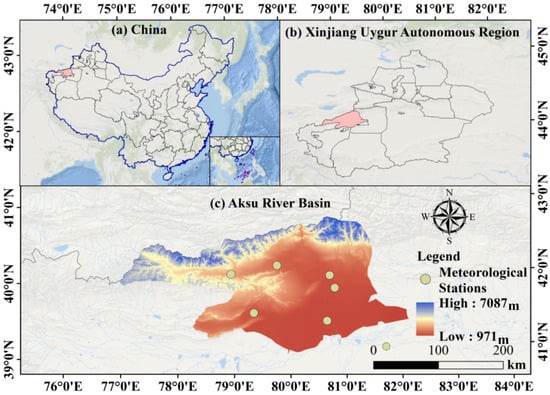
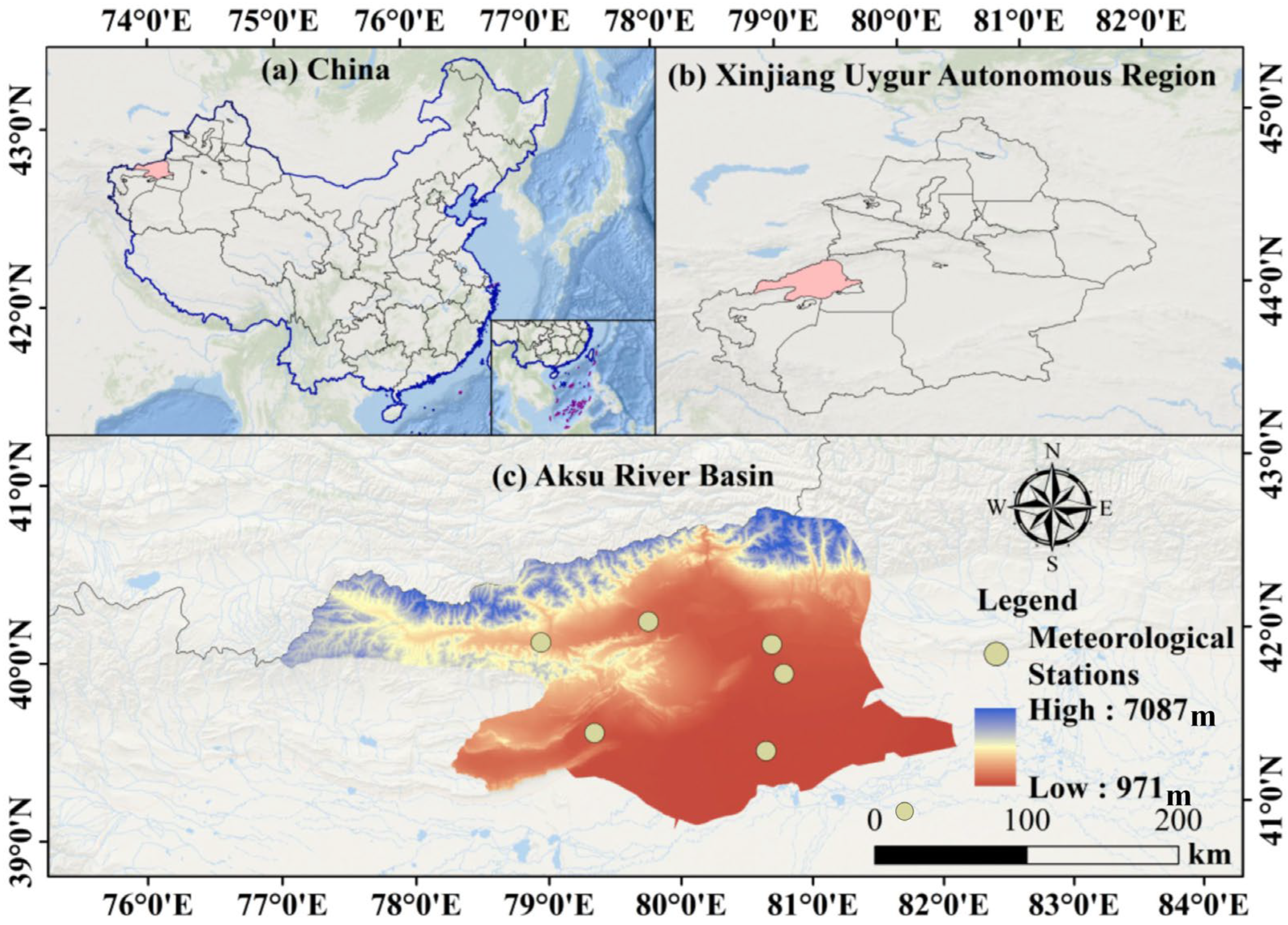
The Aksu River Basin is situated on the northwestern margin of the Tarim Basin, on the southern slopes of the middle Tianshan Mountains in its western part. The terrain within the basin is predominantly characterized by mountains and plains, with an average elevation ranging from 1030 to 1060 m. The topography gradually descends from north to south and from west to east. The total area of the basin is approximately 4.8 × 10⁴ km2 (Figure 1). The Aksu River Basin has a warm temperate arid climate [17], with scarce precipitation and high evaporation. The multi-year average temperature is around 10 °C, and the multi-year average precipitation is 137.7 mm. The Aksu River is a typical mid-latitude high mountain transboundary river, originating in Kyrgyzstan, located between 75°35′ E~82°00′ E and 40°00′ N~42°27′ N. The multi-year average runoff of the main stream of the Aksu River is 63.11 × 10⁸ m3, and the average annual inflow to the basin is 83.08 × 10⁸ m3. The Aksu River supplies 70%~80% of the inflow to the main stream of the Tarim River, making it the largest tributary of the Tarim River [18].
Figure 1.
Location of the study area.
2.2. Data Sources
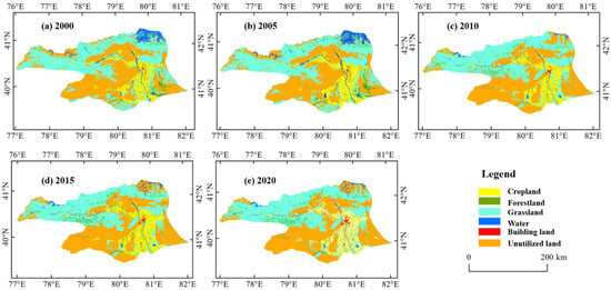
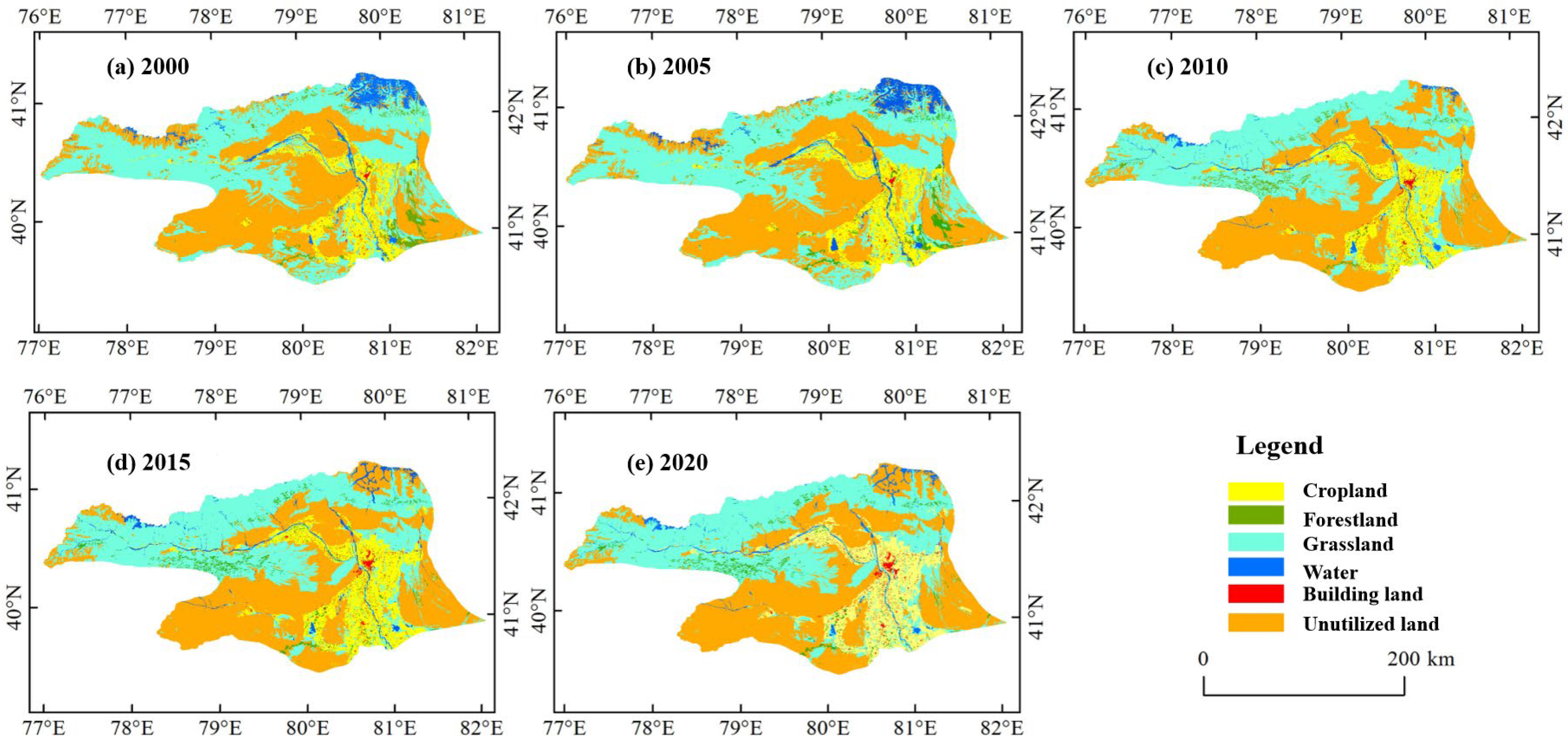
To achieve a comprehensive analysis of evapotranspiration and water consumption characteristics in the Aksu River Basin, this study utilizes multi-source data, including remote sensing products, reanalysis data, ground-based meteorological observations, and land use data. The temporal coverage, spatial resolution, and sources of each dataset are detailed in Table 1. Figure 2 was generated using multitemporal remote sensing-based land use datasets. The original land use data were obtained from publicly available land cover products and were preprocessed through reprojection, spatial clipping to the Aksu River Basin boundary, and class harmonization. The land use classes were then reclassified into six major categories (cropland, forestland, grassland, water, building land, and unutilized land) to ensure consistency across different years. These maps illustrate the spatial distribution and temporal evolution of land use patterns in the Aksu River Basin.
Table 1.
Main data types and sources.
Figure 2.
Distribution of land use types in the Aksu River Basin.
3. Method
3.1. Evapotranspiration Estimation
3.1.1. Penman–Monteith-Based ET0 and ETa Estimation
The Penman–Monteith (P−M) equation is the reference evapotranspiration calculation method recommended by the FAO and is widely applied in hydrological and agrometeorological studies [19]. The FAO Penman–Monteith framework assumes a hypothetical reference surface consisting of a well-watered, uniform grass canopy with a fixed height of 0.12 m, an albedo of 0.23, and a surface resistance of 70 s·m−1. Under these standard boundary conditions, evapotranspiration is controlled by surface energy balance and aerodynamic transport processes. Reference evapotranspiration (ET0) is calculated as:
where T is the mean daily air temperature at 2 m height (°C), Δ is the slope of the saturation vapor pressure curve (kPa·(°C−1), Swnet is the net shortwave radiation flux (MJ·m−2·d−1, Rs is derived from ERA5 reanalysis data), is the net longwave radiation flux (MJ·m−2·d−1), = 0.23, G is the soil heat flux (MJ·m−2·d−1), γ is the psychrometric constant (kPa·(°C−1), is the mean wind speed at 2 m height (m·s−1), is the saturation vapor pressure (kPa), and is the actual vapor pressure (kPa).
Actual evapotranspiration (ETa) was derived from ET0 by incorporating land surface characteristics through land use-dependent coefficients, which account for differences in vegetation type and underlying surface conditions. Specifically, ETa was calculated by multiplying ET0 by surface-specific coefficients corresponding to cropland, grassland, forest, water bodies, and unused land, thereby converting reference evapotranspiration under standard conditions to actual evapotranspiration under real environmental conditions. All meteorological inputs required by the Penman–Monteith equation were obtained from station observations and spatially interpolated to the basin scale prior to calculation.
3.1.2. Remote Sensing-Based ET Estimation
(1) Actual Evapotranspiration Estimation Based on MODIS Product Data
We used the MODIS evapotranspiration product MOD16A2 (Version 6) for the period 2000–2020, which provides day-weighted aggregation of 8-day actual evapotranspiration (ET) estimates at a spatial resolution of 500 m. The MOD16A2 product is based on an improved Penman–Monteith framework, in which actual evapotranspiration is computed as the sum of canopy transpiration, soil evaporation, and wet canopy evaporation [20]. Surface resistance is parameterized using MODIS-derived vegetation variables, including leaf area index (LAI), fraction of photosynthetically active radiation (FPAR), and biome-specific parameters, while meteorological forcing variables (air temperature, humidity, radiation, and wind speed) are obtained from global reanalysis datasets, allowing ET to be estimated under actual land surface conditions rather than as reference evapotranspiration [21]. Following the official product specification, MOD16A2 ET values were converted using the scale factor of 0.1 and filtered using quality control (QC) flags to exclude low-quality or invalid pixels (e.g., cloud contamination or retrieval failure). The 8-day ET data were aggregated to monthly ET using a day-weighted summation, whereby all 8-day composites intersecting a given month were weighted by their effective day counts; annual ET was obtained by summing monthly totals. All MOD16A2 tiles were reprojected to WGS-84, clipped to the Aksu River Basin boundary, and spatially resampled only for grid alignment across datasets, without introducing additional physical spatial detail. Previous studies have demonstrated that MOD16 can reasonably capture the spatiotemporal variability in evapotranspiration in arid and semi-arid regions, although uncertainties may increase over sparsely vegetated surfaces [22,23].
(2) Inversion of Actual Evapotranspiration Based on GRACE Gravity Satellite Data
The inversion of actual evapotranspiration based on GRACE gravity satellite data was conducted using a basin-scale water balance approach. Monthly terrestrial water storage changes (ΔS) were derived from the CSR GRACE mascon solution, which has been widely applied in hydrological studies due to its reduced signal leakage and improved spatial localization compared with spherical harmonic solutions. The CSR mascon monthly product integrates GRACE and GRACE-FO observations under a unified processing framework and provides a temporally consistent TWSA record across the mission transition period. Therefore, no additional interpolation or gap-filling procedure was applied in this study. Precipitation (P) was obtained from gridded gauge-based meteorological datasets, and runoff (R) was derived from hydrological observations and model-based estimates aggregated at the basin scale. Actual evapotranspiration was then reconstructed as ET = P – R − ΔS, where the residual term represents combined measurement and processing uncertainties. It should be noted that uncertainties in precipitation inputs, runoff regulation (including reservoir operations and irrigation return flows), boundary flux assumptions, and GRACE storage retrieval errors inevitably propagate into the residual ET estimate. However, these uncertainty sources exhibit heterogeneous error structures and limited covariance information at the basin scale, making formal component-wise uncertainty propagation difficult to implement without introducing pseudo-precision. In this study, water balance ET derived from GRACE is therefore interpreted as a large-scale integrated constraint rather than a fully resolved monthly closure estimate. Although uncertainties in precipitation, runoff, and GRACE storage changes inevitably propagate into water balance ET estimates, these effects primarily influence short-term variability and are reduced when analyzing seasonal and inter-annual basin-scale signals. Considering that the area of the Aksu River Basin is smaller than the effective GRACE footprint, GRACE-based ET in this study is used to characterize integrated basin-scale water balance constraints rather than local spatial heterogeneity. Within the probabilistic BMA framework, the component-specific variance term associated with GRACE-based ET is explicitly estimated through the likelihood function. Ensemble members exhibiting larger discrepancies or higher uncertainty are assigned lower effective weights, and their uncertainty contributions are reflected in the predictive variance of the integrated ETa estimate. In this sense, GRACE-related uncertainty is statistically accommodated within the ensemble fusion rather than ignored. Within the multi-source framework of this study, GRACE-based ET serves as an independent constraint and is further integrated with other ET estimates using Bayesian Model Averaging, which effectively reduces sensitivity to uncertainties associated with individual water balance components [24,25,26]:
where ETa is reconstructed actual evapotranspiration, mm; P is precipitation, mm; R is runoff depth, mm; ∆S is the variation in monthly terrestrial water storage, mm; and represents residual errors arising from measurement uncertainty, leakage correction, unaccounted boundary fluxes, and human regulation. In this study, is not explicitly quantified; therefore, GRACE-based ET is interpreted as a basin-scale water balance residual primarily constraining seasonal and inter-annual variability rather than exact monthly ET magnitude.
(3) Estimation of Actual Evapotranspiration Based on the GLDAS–Noah Model
This study utilizes monthly actual evapotranspiration (ETa) data from the GLDAS-2.1–Noah land surface model for the period 2000–2020, with a native spatial resolution of 0.25° × 0.25°. GLDAS–Noah is a physically based land surface model that simulates evapotranspiration through surface energy and water balance processes driven by meteorological forcing, rather than a remote sensing-based product. The GLDAS-2.1–Noah dataset used in this study does not incorporate data assimilation and represents model-simulated land surface fluxes forced by observation-based atmospheric inputs. Using the “Multidimensional Tools” in ArcGIS 10.6, monthly GLDAS data were batch-converted to raster format and resampled to 500 m using cubic convolution interpolation solely for spatial alignment and visualization purposes. For intercomparison and BMA fusion, GLDAS ETa was used at its native 0.25° resolution or at basin-aggregated temporal scales, and any 500 m resampling was applied only for grid alignment and visualization, without introducing additional physical spatial detail. This resampling did not introduce new spatial information and was not intended as physical downscaling; all analyses involving GLDAS–Noah ETa were conducted at basin or aggregated scales. The data were then clipped to the Aksu River Basin to extract monthly ETa values for subsequent analysis. It should be noted that GLDAS–Noah ETa shares meteorological forcing inputs with other ET reconstructions (e.g., precipitation), which may introduce statistical dependence when multi-source products are jointly integrated.
3.1.3. Multi-Model Integration Based on Bayesian Model Averaging (BMA)
Bayesian Model Averaging (BMA) is a probabilistic ensemble framework widely used to integrate predictions from multiple models while explicitly accounting for inter-model variability and uncertainty. Rather than aiming to improve prediction accuracy, BMA is designed to provide a statistically consistent representation of model agreement and uncertainty across ensemble members [27]. In the absence of direct basin-scale observations of actual evapotranspiration (ETa) in the study region, BMA was employed to generate an ensemble-consistent ETa estimate by integrating multiple ETa products relative to a reference time series, rather than to calibrate or improve absolute prediction accuracy. The BMA predictive distribution of ETa can be expressed as:
where y represents the multi-model integration result; represents the simulated values of the K models; yT denotes a reference ETa time series used for relative consistency evaluation rather than true observations, due to the lack of direct basin-scale ETa measurements in the study region; represents the posterior probability of the simulated values of the kth model, i.e., the model weight; and denotes the conditional probability density function associated with the simulated results of an individual model. The expectation and variance in the BMA multi-model integration are respectively given by:
where denotes a normal distribution with mean and variance .
In this study, a Gaussian likelihood function was adopted for each model component, and the BMA weights and variances were estimated using maximum likelihood estimation implemented via the expectation–maximization (EM) algorithm. However, potential dependence among ensemble members and bias in GRACE-based ET require careful consideration. We acknowledge that some ETa products are not strictly independent because they may share common forcing datasets or auxiliary components (e.g., precipitation, runoff, or model-based storage terms). In particular, GRACE-based water balance ET and GLDAS–Noah ET may exhibit statistical dependence through shared hydrometeorological inputs, which can violate the strict conditional independence assumption of classical BMA and potentially lead to the overweighting of correlated information. To mitigate this risk, BMA was implemented at the basin scale with seasonal–annual aggregation, and the model weights were estimated as global and temporally invariant rather than calibrated at the pixel/monthly level. This design reduces the influence of shared short-term forcing noise and limits the dominance of any single correlated component in the fused estimate. Accordingly, the BMA-derived ETa was interpreted as an ensemble-consistent estimate of product agreement under uncertainty, rather than a calibrated improvement against independent “truth”. It should be emphasized that the reference series adopted in the BMA formulation was not treated as a surrogate for “true” evapotranspiration. Instead, it served solely as a statistical consistency benchmark in the absence of basin-scale ETa observations. The estimated BMA weights, therefore, quantify the relative statistical agreement of ensemble members rather than their physical credibility.
In addition, the BMA weights were estimated at the basin scale and assumed to be temporally invariant after seasonal–annual aggregation. This structurally constrained and low-dimensional implementation limits model flexibility and reduces potential sensitivity to short-term variability or individual-member bias. Under this formulation, the BMA result represents a stabilized ensemble representation rather than a reference-driven calibration.
GRACE-based water balance ET is inherently sensitive to uncertainties in precipitation and runoff forcing, GRACE solution errors (e.g., leakage and spatial smoothing), and assumptions involved in storage change estimation. As a result, it may exhibit systematic deviations and occasional nonphysical fluctuations at the monthly scale. Within the probabilistic BMA framework, such deviations are accommodated through the likelihood estimation and component variance terms: models with larger discrepancies or higher uncertainty are assigned lower effective weights and contribute proportionally to the predictive uncertainty of the integrated ETa estimate. In this sense, GRACE is used primarily as a large-scale water balance consistency constraint rather than as a definitive reference for ET magnitude. To avoid overfitting and to ensure physical interpretability under data-sparse conditions, the BMA weights were assumed to be spatially aggregated at the basin scale and temporally invariant over the study period, rather than estimated at individual grid cells or stations.
Because the ETa datasets integrated within the BMA framework have substantially different native spatial resolutions (GRACE at >1°, GLDAS at 0.25°, and MODIS at 500 m), model fusion was conducted at the basin scale and seasonal–annual temporal scales rather than at the native pixel level. This strategy minimizes double-counting of spatial information and prevents artificial dominance of higher-resolution products. Within the BMA framework, GRACE and GLDAS primarily constrain large-scale water balance consistency, whereas MODIS provides complementary information on land surface heterogeneity, which is incorporated through basin-scale and seasonal–annual aggregation rather than pixel-level fusion. BMA was adopted because it provides a transparent probabilistic framework for integrating multiple ETa products while explicitly representing model uncertainty and relative agreement among ensemble members [28]. Unlike GLUE-based methods that rely on subjective likelihood definitions [29], or machine learning fusion approaches that require large training datasets and may lack physical interpretability [30], BMA determines model weights statistically and remains physically consistent and data-efficient. These characteristics make BMA particularly suitable for ETa fusion in arid inland river basins with sparse observations and strong surface heterogeneity [31]. Importantly, the BMA-derived ETa in this study is interpreted as an ensemble-consistent estimate rather than a calibrated improvement against true measured evapotranspiration.
3.2. Theil–Sen Median Trend Analysis
The Theil–Sen Median trend analysis method performs trend analysis using the median of time series data points. It is primarily applied for trend analysis of evapotranspiration time series data at the pixel scale [32]. The calculation formula is as follows:
where Sj and Si represent the data corresponding to the i-th and j-th years in the study period. ( ) denotes the median value. A trend coefficient result of β > 0 indicates an increasing trend in the time series data, while β < 0 indicates a decreasing trend.
3.3. Mann–Kendall Test
The Mann–Kendall test is a nonparametric test used for trend analysis in time series data. The formula is as follows [33]:
where Z is the standardized test statistic, S is the test statistic, xi and xj are the evapotranspiration values for the i-th and j-th years, respectively, and n is the length of the time series data (in this study, n = 21).
Under a given significance level, a two-tailed trend test is conducted by referring to the critical value Z1−α/2 from the standard normal distribution table. When |Z| ≤ Z1−α/2, the null hypothesis is accepted, indicating that the trend is not significant. If |Z| > Z1−α/2, the null hypothesis is rejected, implying that the trend is considered significant. This study selected significance levels of α = 0.05 and α = 0.10 for significance testing, with corresponding Z1−α/2 values of ±1.96 and ±1.65. By integrating the β and Z values, the trends in ETa were classified into five categories: significant increase, slight increase, no change, slight decrease, and significant decrease. Because the trend test was applied to the annual ETa series, the influence of serial correlation was reduced; therefore, no prewhitening was applied [34,35].
Although the primary analyses were conducted at the basin-wide scale, preliminary sub-regional checks based on major physiographic units (upper/middle/lower reaches and mountain–oasis–desert patterns) indicated consistent temporal trends, supporting the use of cumulative basin-scale analysis in this study. Basin-wide aggregation was therefore adopted to ensure statistical robustness and comparability across time.
3.4. Evaluation of Water Consumption Effectiveness
Based on the ecosystem water use efficiency model [36], evapotranspiration is categorized as follows: high-efficiency water consumption (significantly contributing to ecological restoration/vegetation growth); medium-efficiency water consumption (mixed vegetation–ground water consumption); and low-efficiency water consumption (evaporation from barren desert lands, with minimal ecological contribution). This classification is based on the functional contribution of evapotranspiration to ecosystem services and land surface processes, rather than on fixed numerical thresholds, and reflects differences in water use effectiveness among underlying surface types. The calculation formula is as follows:
where Wi is the water consumption of the i-th underlying surface type, ETai is the evapotranspiration per unit area, and Ai is the land use area.
Evaluation Indicators of Water Consumption Effectiveness Structure:
Ultimately, the dual-scale evaluation of water consumption structure at both the watershed and irrigation district levels is achieved.
All ETa values are reported in mm (monthly) and mm/a (annual), where ETa is in mm and A is area in m2, yielding W in m3; the results are also expressed in 108 m3 for readability.
4. Analysis
4.1. Multi-Source Actual Evapotranspiration Estimation Results and Model Accuracy Validation
4.1.1. Actual Evapotranspiration in the Aksu River Basin (2000–2020)
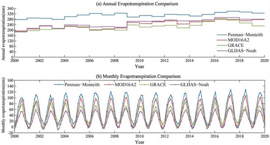
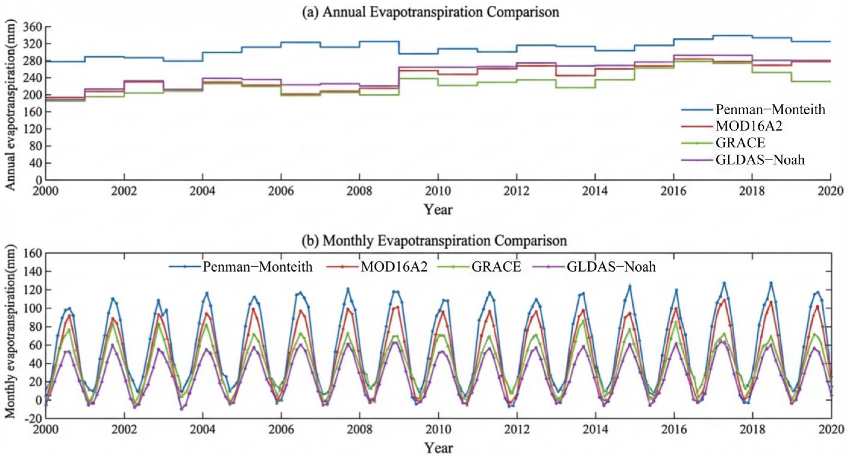
Based on the Penman–Monteith (P-M) method and multiple remote sensing/reanalysis datasets, the actual evapotranspiration (ETa) in the Aksu River Basin from 2000 to 2020 was estimated, and the results are shown in Figure 3. According to the P-M results (Figure 3), the multi-year average ETa in the Aksu River Basin was 311.22 mm. Inter-annually, ETa generally exhibited an increasing trend, with a growth rate of 2.27 mm/a. The maximum and minimum annual ETa values occurred in 2018 and 2000, respectively. The maximum value reached 341.61 mm, which was 30.39 mm higher than the multi-year average (a relative increase of 9.76%), whereas the minimum value was 279.00 mm, 32.22 mm lower than the multi-year average (a relative decrease of 10.35%). On the intra-annual scale, ETa exhibited a significant unimodal seasonal pattern (Figure 3). ETa increased continuously from January to July, reaching its peak in July or August, and then gradually decreased thereafter. The minimum values typically occurred in January and December. In addition to the P-M estimates, ETa was also derived from MOD16A2, GRACE gravity satellite data, and the GLDAS–Noah model (Figure 3). The results indicate significant differences among data sources in terms of numerical magnitude, inter-annual variability, and seasonal distribution characteristics. The multi-year average ETa estimated from MOD16A2 was 162.54 mm, notably lower than those derived from other methods, but it exhibited a sustained upward trend with an annual growth rate of 3.68 mm/a. At the intra-annual scale, MOD16A2 ETa also showed a pronounced unimodal distribution, increasing from January to July, peaking in July–August, and gradually declining thereafter. Summer (June–July) accounted for approximately 40% of the annual total. However, relatively lower estimates were observed during the high-evapotranspiration period from April to October, while varying degrees of overestimation occurred from November to March of the following year. The multi-year average ETa reconstructed from GRACE was 255.77 mm, exhibiting substantial inter-annual variability. Monthly variations followed a similar unimodal pattern, although apparent negative values occurred in some months, reflecting uncertainties associated with gravity inversion and water balance assumptions in arid regions. The GLDAS–Noah model produced a multi-year average ETa of 244.43 mm, which lies between the MOD16A2 and GRACE estimates. It exhibited a significant increasing trend at a rate of 3.34 mm/a, with the highest annual value occurring in 2016 (309.67 mm) and the lowest in 2000 (191.52 mm), indicating pronounced inter-annual variability. Seasonal variations were also unimodal, with summer evapotranspiration being the strongest (approximately 130 mm on average), followed by spring and autumn, and winter being the weakest. As shown in Figure 3, although the absolute magnitudes differ among datasets, all products consistently capture the dominant seasonal cycle and the overall increasing trend in basin-scale ETa. The differences primarily reflect variations in model structure and physical constraints. Energy balance-driven approaches (P-M and MOD16A2) respond more directly to meteorological forcing, whereas GRACE-based estimates are sensitive to monthly terrestrial water storage changes and signal leakage/smoothing effects, which may shift extrema and amplify inter-annual variability. In contrast, GLDAS–Noah integrates meteorological forcing with land surface processes, resulting in intermediate magnitude and variability characteristics.
Figure 3.
Spatiotemporal patterns of actual evapotranspiration (ETa) in the Aksu River Basin (2000–2020) from multiple data sources.
4.1.2. Model Accuracy Verification
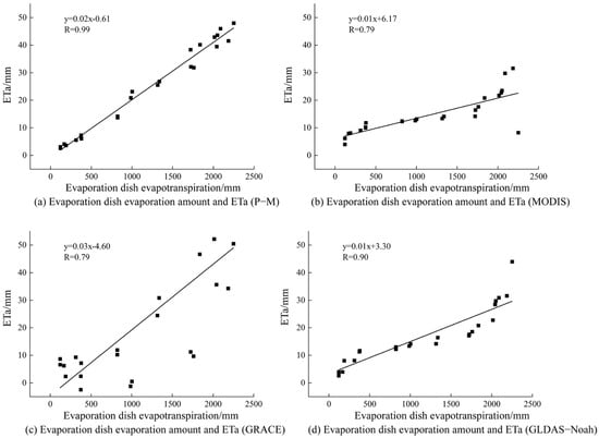
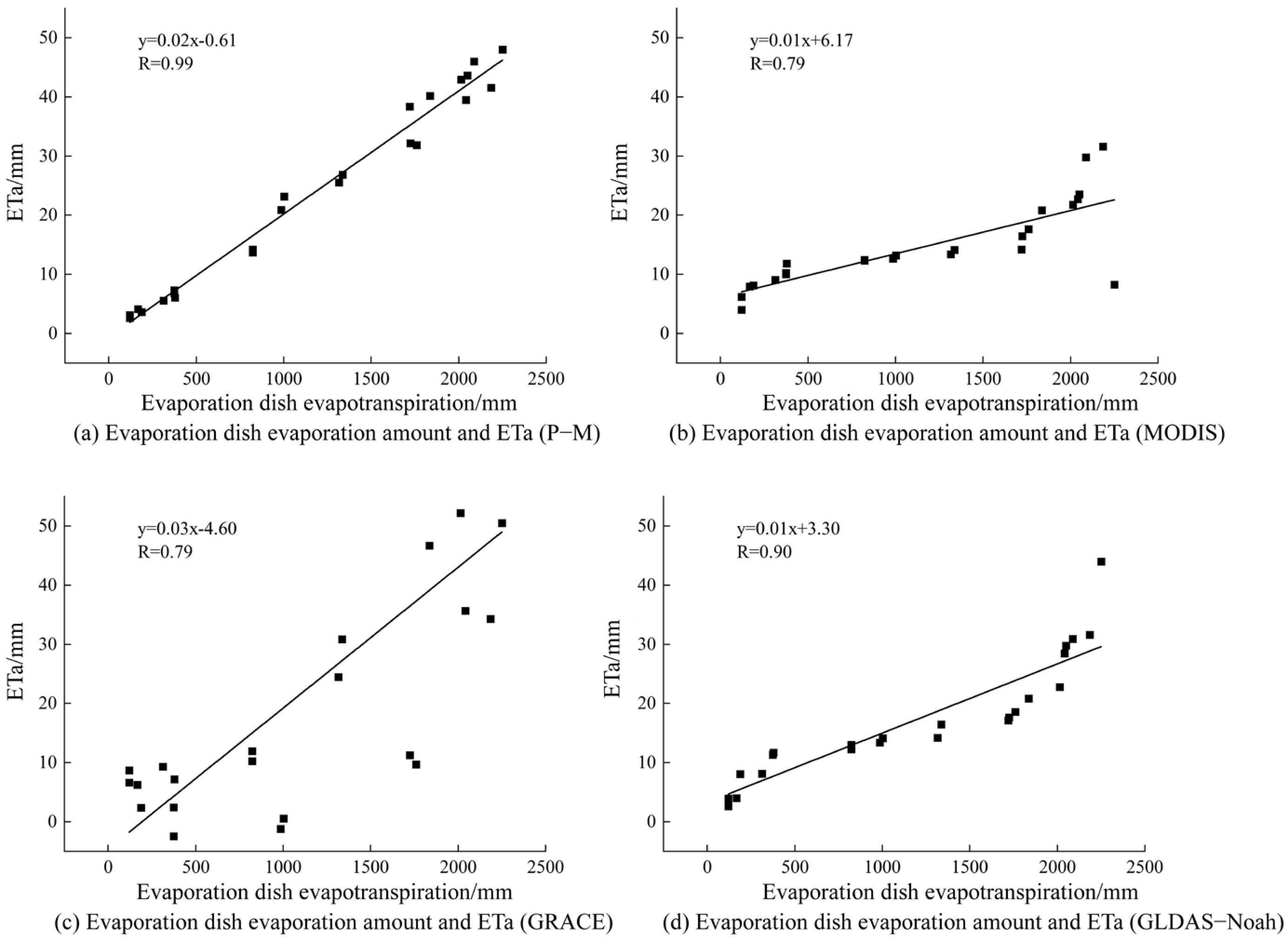
This study selected evapotranspiration data from E601 large-scale evaporation pans at seven meteorological stations within the Aksu River Basin to evaluate the performance of different ETa products (Figure 4). It should be noted that pan evaporation represents atmospheric evaporative demand and generally exceeds actual evapotranspiration because surface resistance and vegetation regulation are not explicitly considered. As a result, pan evaporation and land surface ETa are not physically equivalent, especially in irrigated and vegetated areas typical of arid inland river basins. Therefore, E601 pan data were used as an independent reference to assess temporal consistency and relative model performance rather than as a direct proxy for ETa magnitude. Pan evaporation was used to evaluate temporal consistency and relative variability, not ETa magnitude or absolute accuracy. Accordingly, correlation analysis was employed to evaluate temporal coherence between modeled ETa and pan evaporation. Metrics such as the Nash–Sutcliffe Efficiency (NSE) or Kling–Gupta Efficiency (KGE) were not applied, as they assume direct comparability in magnitude and variance between simulated and observed variables, which is not physically satisfied when using pan evaporation as a reference for ETa. Under such scale mismatch and systematic magnitude differences, the application of amplitude-based error metrics (e.g., RMSE, MBE, NSE, or KGE) may produce misleading interpretations by penalizing structural differences arising from physical non-equivalence rather than model deficiency. Therefore, the evaluation framework adopted here emphasizes temporal coherence, inter-annual variability, and seasonal phase consistency as physically defensible criteria for comparison. In addition to correlation analysis, a diagnostic comparison of seasonal mean anomalies was conducted to examine whether the relative seasonal variability in different ETa products is consistent with that of pan evaporation. Monthly ETa and pan evaporation series were aggregated into seasonal means, and the relative differences in seasonal amplitude and phase were inspected. Because pan evaporation does not represent land surface ETa, these differences are not interpreted as quantitative bias or accuracy errors, and, therefore, RMSE or MBE metrics were not reported. Instead, this diagnostic check serves as a complementary evaluation of relative variability and temporal coherence beyond correlation alone. The comparison results show that the Penman–Monteith model exhibits the highest correlation with pan observations (R ≈ 0.99), followed by GLDAS–Noah (R ≈ 0.90), while MODIS- and GRACE-derived ETa show correlation coefficients of approximately 0.79. These results indicate that all ETa products capture the dominant temporal variability in evaporative processes in the region, despite potential differences in absolute magnitude. The consistency in inter-annual trend direction and seasonal phase across products further supports the interpretation that the integrated ETa series captures large-scale atmospheric forcing signals rather than attempting to reproduce exact magnitude equivalence. However, no individual ETa product alone is sufficient to fully characterize evapotranspiration dynamics under complex surface conditions in arid environments. Because true basin-scale ETa observations are unavailable, the subsequent BMA-derived ETa should be interpreted as an ensemble-consistent estimate rather than a calibrated product against measured truth. Consequently, Bayesian Model Averaging (BMA) was applied to integrate multi-source ETa estimates, thereby reducing systematic model-specific biases and improving the robustness of subsequent spatiotemporal analysis and water consumption assessment.
Figure 4.
Relationship between evapotranspiration from evaporimeters at weather stations and ETa. (a) P−M, (b) MODIS, (c) GRACE, and (d) GLDAS−Noah. Black dots represent observed values, and the solid line indicates the linear regression fit. The regression equation and correlation coefficient (R) are shown in each panel.
4.2. Spatiotemporal Variation Characteristics of Actual Evapotranspiration
4.2.1. Characteristics of Time Scale Variations
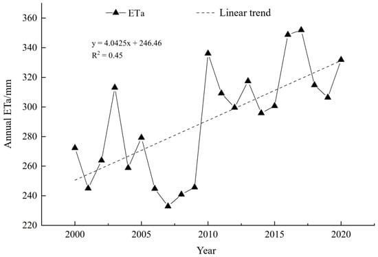
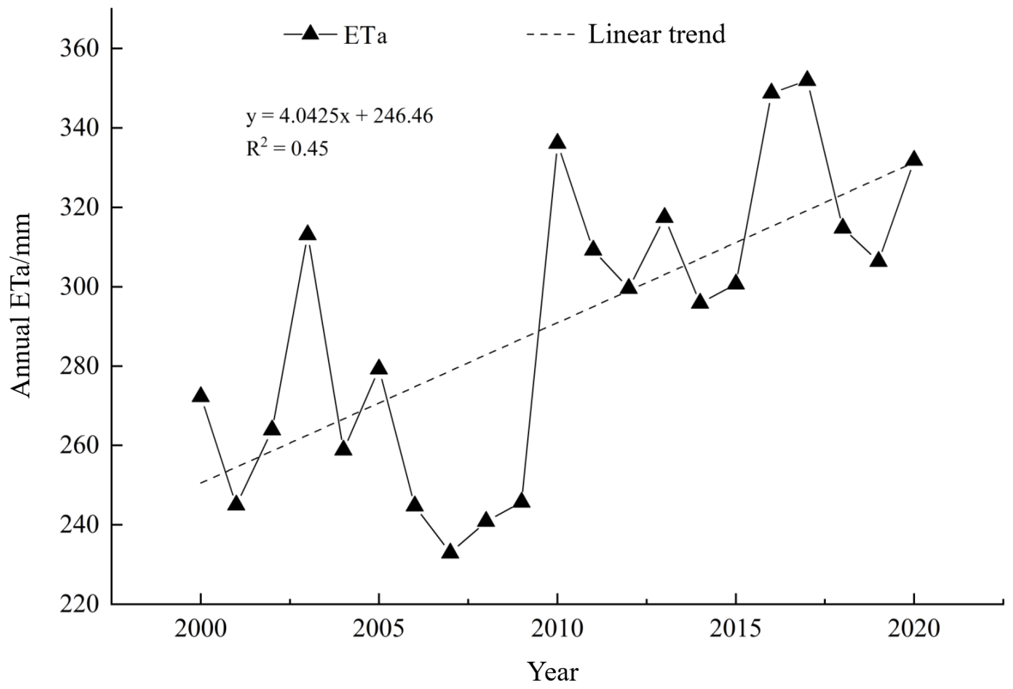
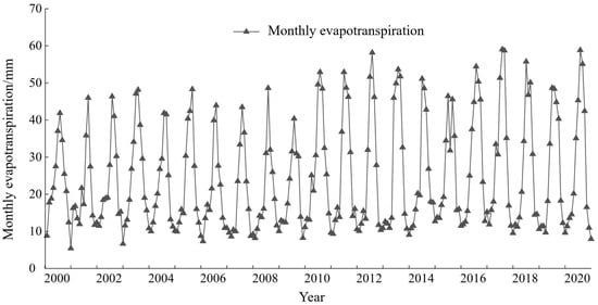
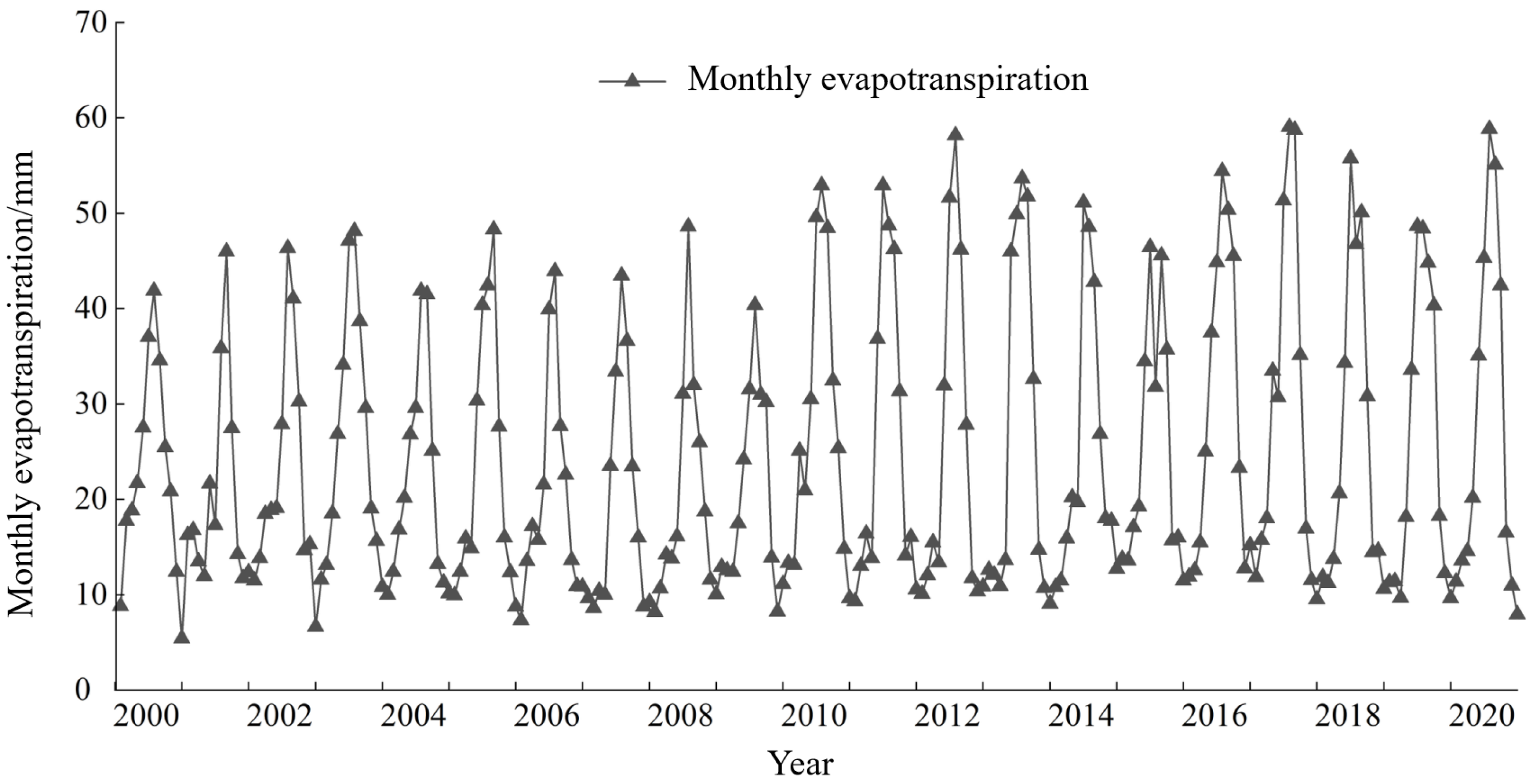
Based on data from seven meteorological stations in the Aksu River Basin from 2000 to 2020, the actual evapotranspiration (ETa) of the basin was calculated using the integrated BMAMN model. As shown in Figure 5 and Figure 6, the results indicate that from 2000 to 2020, the ETa in the Aksu River Basin exhibited a significant overall upward trend, with a multi-year average of 290.93 mm and a growth rate of 4.04 mm/a. Since all individual ET products exhibit a consistent positive inter-annual trend over the study period, and the BMA fusion is mathematically a convex combination of ensemble members, the long-term trend direction of the fused series is structurally stable. In terms of intra-annual variation, ETa displayed a distinct unimodal distribution pattern. Approximately 79.54% of the annual evapotranspiration was concentrated from April to October, with the peak period occurring in July–August. This aligns closely with the period of highest regional temperatures, peak vegetation growth, and the most intensive irrigation water use.
Figure 5.
Annual variation in average actual evapotranspiration in the Aksu River Basin from 2000 to 2020.
Figure 6.
Monthly variations in actual evapotranspiration in the Aksu River Basin, 2000–2020.
4.2.2. Characteristics of Spatial-Scale Variation
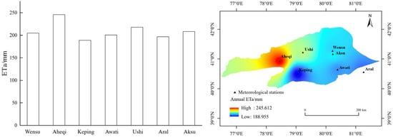
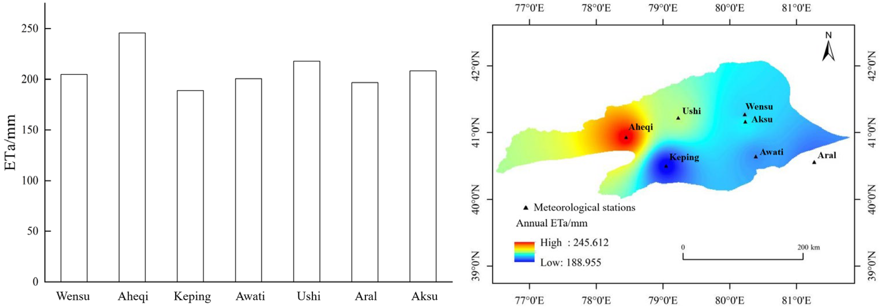
Based on the results of multi-year average actual evapotranspiration (ETa) calculated using the BMAMN model for seven meteorological stations in the Aksu River Basin (Figure 7), significant spatial differences in ETa across the basin are evident. Among the stations, Aheqi County recorded the highest ETa at 245.61 mm/a, while Kalpin County recorded the lowest at 188.95 mm/a. The ETa values for the remaining stations are as follows: Wushi County at 217.95 mm/a, Aksu City at 208.34 mm/a, Wensu County at 204.82 mm/a, Awat County at 200.60 mm/a, and Aral City at 196.87 mm/a. Spatial interpolation using the inverse distance weighting (IDW) method based on the station ETa data revealed that the overall spatial distribution of ETa in the Aksu River Basin exhibits a clear pattern of “higher in the northwest and lower in the southeast”, with a gradient characteristic where average evapotranspiration decreases from upstream to midstream and further to downstream.
Figure 7.
Spatial distribution of multi-year average ETa in the Aksu River Basin.
The inverse distance weighting (IDW) method was selected for spatial interpolation because of the limited number of meteorological stations available in the Aksu River Basin and the primary objective of illustrating basin-scale spatial gradients rather than precise local prediction. IDW does not require assumptions regarding spatial stationarity or variogram structure, which are difficult to robustly estimate under sparse observation conditions. Given the sparse and uneven station distribution, the interpolated surface should be interpreted as a descriptive visualization of large-scale spatial tendencies rather than as a high-precision predictive product. The interpolation results are not used as independent inputs in subsequent modeling, statistical inference, or ensemble fusion procedures. Instead, they serve to illustrate basin-scale upstream–downstream contrasts and to support qualitative interpretation of spatial differentiation patterns. The identified northwest–southeast gradient is therefore interpreted as a basin-scale feature that corresponds to climatic conditions, topography, and land surface characteristics, while the influence of the specific interpolation method on the overall spatial pattern is limited. High ETa values are predominantly concentrated in the northwestern regions of Aheqi County and Wushi County, while low ETa values are mainly distributed in Kalpin County and the surrounding areas of Aral City. Because the principal conclusions of this study are derived from temporal trend analysis and multi-source ETa fusion rather than from interpolated surfaces, potential interpolation uncertainty is unlikely to affect the basin-scale gradient structure emphasized here.
This spatial ETa gradient is consistent with the combined effects of topography, climate, vegetation distribution, and irrigation intensity across the basin. The northwestern upstream regions are characterized by higher elevations and are influenced by orographic precipitation and snowmelt supply from the Tianshan Mountains, providing relatively sufficient water availability for evapotranspiration. These areas also exhibit denser natural vegetation and more intensive oasis irrigation, both of which may be associated with higher ETa. In contrast, the southeastern downstream regions are dominated by low-lying desert landscapes with limited precipitation, sparse vegetation cover, and weaker irrigation influence, resulting in lower ETa values. Therefore, the observed “northwest high–southeast low” pattern represents a basin-scale spatial differentiation that corresponds with natural climatic gradients and human water use activities within the Aksu River Basin.
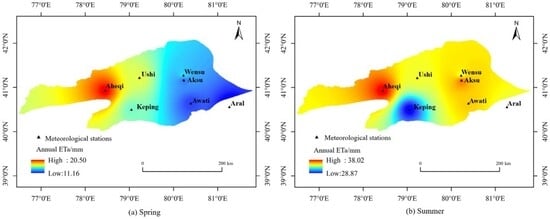
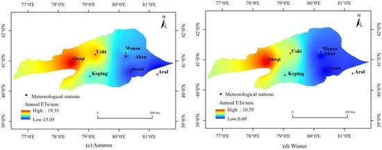
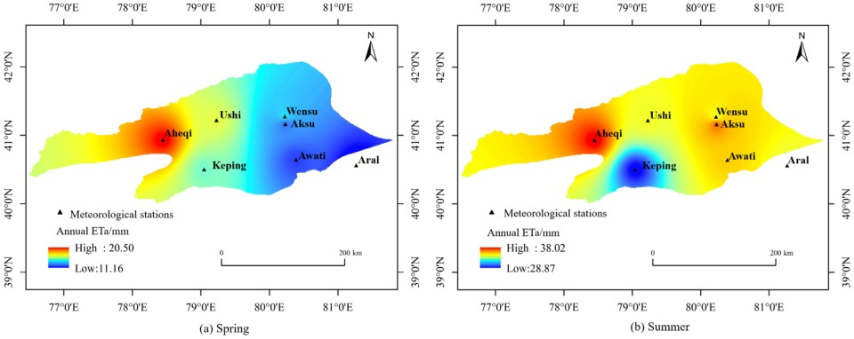
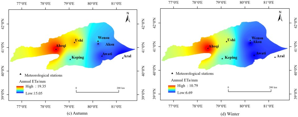
The spatial distribution of actual evapotranspiration (ETa) across the Aksu River basin throughout the four seasons is shown in Figure 8. Its overall spatial pattern largely aligns with the characteristics of the multi-year average ETa distribution, exhibiting a spatial gradient where upstream areas show higher values than midstream, and midstream areas show higher values than downstream. On a seasonal scale, spring ETa remains generally low, though upstream regions already display relatively high evapotranspiration values. Summer ETa reaches its annual peak across the entire basin, with significantly expanded high-value zones. Autumn ETa decreases markedly from summer levels yet maintains consistent spatial distribution patterns. Winter ETa remains at its annual minimum across all regions, with relatively diminished spatial variation. Overall, ETa in the Aksu River Basin exhibits pronounced seasonal variations throughout the year, while its spatial distribution demonstrates strong consistency across different seasons.
Figure 8.
Spatial distribution of multi-year quarterly ETa averages in the Aksu River Basin.
4.2.3. Spatial Change Trends
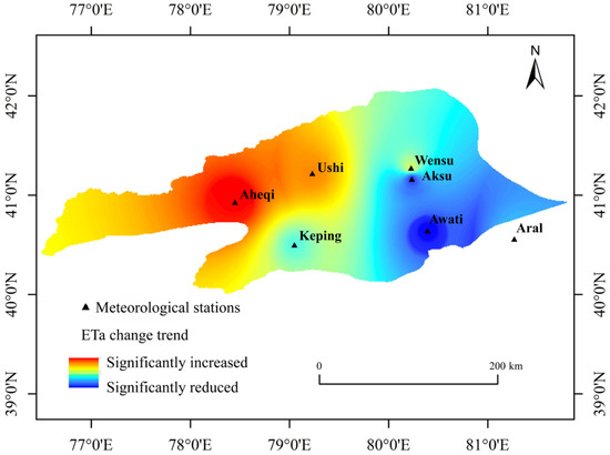
Based on annual actual evapotranspiration (ETa) data from seven meteorological stations in the Aksu River basin, the Theil–Sen slope estimation and Mann–Kendall (M-K) trend tests were applied. Combined with inverse distance weighting (IDW) for spatial visualization of basin-scale trend patterns, the spatial distribution characteristics of ETa trends in the basin from 2000 to 2020 were obtained (Table 2, Figure 9). The results indicate that ETa exhibited an overall increasing tendency during the study period. Areas with increasing ETa covered 43.22% of the basin, with significantly increasing areas accounting for 20.44%. These were primarily concentrated in Aheqi County and Ush County in the basin’s northwest, displaying a continuous zonal spatial distribution pattern. Areas with decreasing ETa accounted for 40.08%, with significantly decreasing areas covering 21.41% and primarily distributed in Aksu City and Awati County in the southeastern part of the basin. The remaining 16.70% of the area showed no significant change in ETa, mostly concentrated in the northern, southern, and eastern parts of the basin. Overall, the spatial variation in ETa in the Aksu River basin demonstrates a west-to-east differentiation in trend magnitude, with relatively stronger increasing tendencies in the western region, limited changes in parts of the central area, and localized decreasing tendencies in some eastern areas.
Table 2.
Statistical analysis of ETa trends in the study area from 2000 to 2020.
Figure 9.
Spatial analysis of ETa trends in the Aksu River Basin from 2000 to 2020.
4.3. Water Consumption Characteristics and Effectiveness Evaluation
4.3.1. Actual Evapotranspiration Characteristics of Various Land Use Types
Actual evapotranspiration (ETa) derived from the integrated BMAMN model was statistically analyzed for different land use types in 2000, 2005, 2010, 2015, and 2020 (Table 3). Clear and persistent differences were observed among land use categories. Grassland exhibited the highest multi-year average ETa (245.86 mm/a), followed by cropland (236.94 mm/a) and forest land (221.30 mm/a), whereas unutilized land showed the lowest value (143.05 mm/a). The ranking of ETa magnitude remained stable across benchmark years: grassland > cropland > forest land > unutilized land. Given that grassland accounts for 40.35% of the basin area, it contributes the largest share to total basin evapotranspiration. In contrast, unutilized land consistently exhibits lower ETa, reflecting sparse vegetation cover and limited surface water use. Overall, ETa in the Aksu River Basin demonstrates a clear and structurally stable gradient differentiation across land use types. In this study, land use-specific ETa contrasts provide the basis for a structural classification of water consumption efficiency at the basin scale. This classification represents relative differentiation in evapotranspiration intensity among surface types rather than a direct quantification of ecohydrological efficiency, transpiration fraction, or water productivity. The objective is to characterize basin-scale structural contrasts in water consumption patterns under heterogeneous land cover and irrigation conditions. Land use ETa patterns primarily reflect spatial variability captured by MODIS-based retrievals, while GLDAS and GRACE constrain large-scale temporal consistency. Vegetation activity proxies such as NDVI are implicitly incorporated within the MODIS ET algorithm and provide ecological context consistent with the observed ranking: land use types with denser canopy cover and longer growing seasons generally exhibit higher ETa, whereas sparsely vegetated surfaces maintain persistently lower values. To quantify inter-annual variability, the mean ± standard deviation across benchmark years was calculated as follows: cropland: 236.94 ± 12.47 mm/a, forest land: 221.30 ± 20.81 mm/a, grassland: 245.86 ± 21.13 mm/a, and unutilized land: 143.05 ± 10.65 mm/a. Between-class contrasts in ETa magnitude exceed within-class inter-annual fluctuations, further supporting the robustness of structural differentiation at the basin scale.
Table 3.
Annual average ETa of land use types in the Aksu River Basin from 2000 to 2020. Unit: mm/a.
4.3.2. Water Consumption Characteristics of Different Land Use Types
Based on land use-specific ETa and corresponding surface areas, total water consumption was calculated for each land use category (Table 4). The results indicate clear structural differences in basin-scale water consumption. Grassland contributes the largest share of total water consumption (48.91% on average), followed by unutilized land (30.24%) and cropland (14.59%), whereas forest land accounts for the smallest proportion (2.69%). Although unutilized land exhibits relatively low per-unit ETa intensity, its extensive spatial coverage results in a substantial contribution to total basin water consumption. In contrast, cropland and forest land show higher ETa intensity per unit area but contribute a smaller proportion to total water consumption due to their comparatively limited spatial extent. These findings indicate that basin-scale water consumption structure is closely associated with both evapotranspiration intensity and land use distribution. Across the five benchmark years, the proportional contribution of each land use category remains generally stable, indicating persistent structural characteristics in water consumption patterns. The dominance of grassland and unutilized land in total water consumption underscores the structural importance of surface-type composition in shaping basin-scale evapotranspiration patterns.
Table 4.
Water consumption calculation results for land use types in the Aksu River Basin.
4.3.3. Water Use Efficiency Evaluation
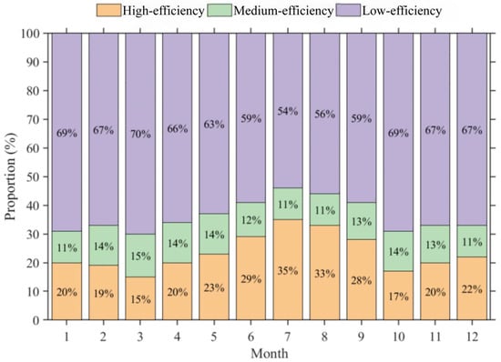
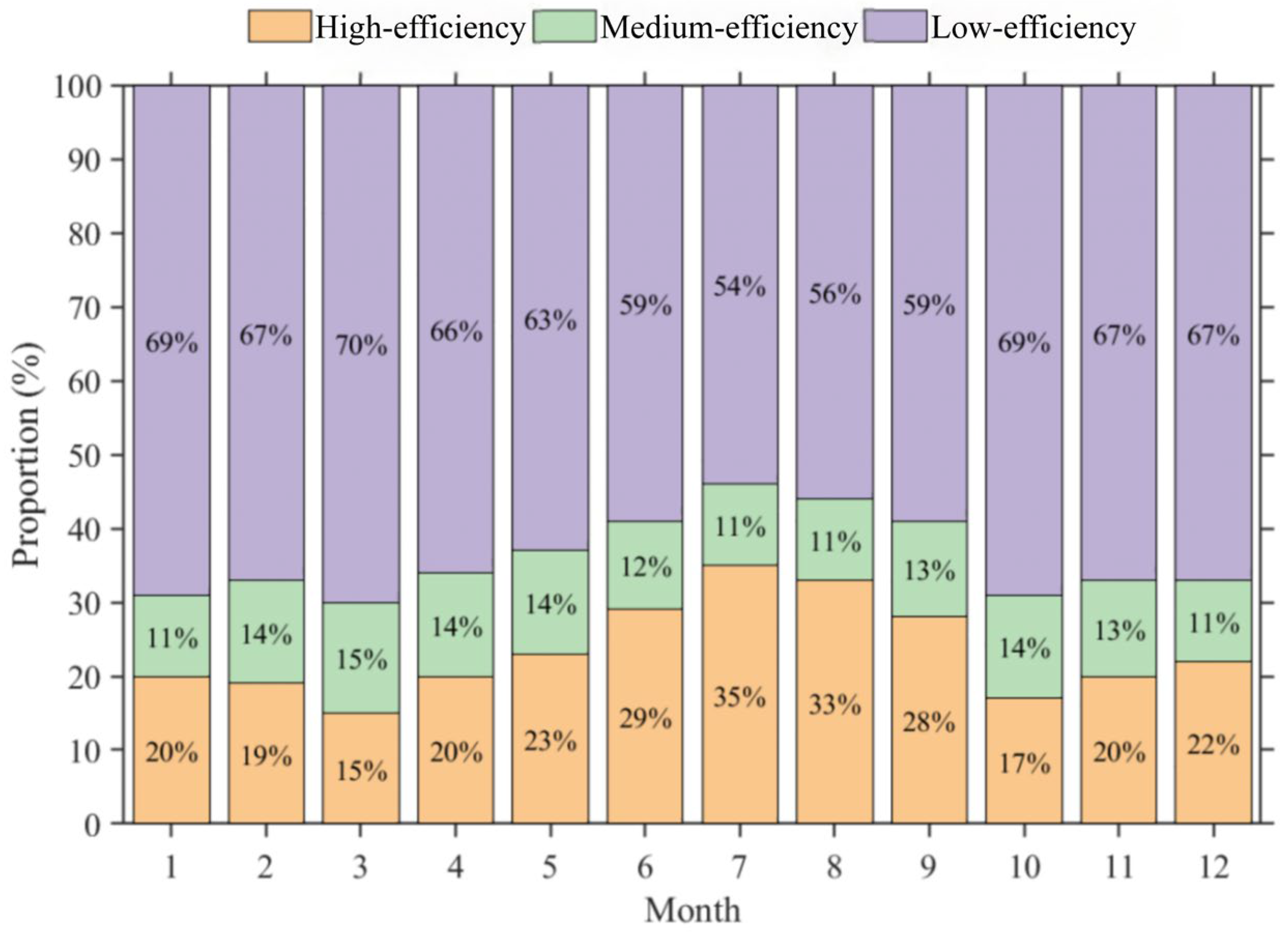
In this study, water use efficiency is defined as a structural classification of evapotranspiration-based water consumption among land use types at the basin scale, rather than as a ratio-based ecohydrological efficiency metric or a direct process-based partitioning between transpiration and evaporation. Forestland and grassland are classified as high-efficiency water use due to stable vegetation cover and relatively higher vegetation-associated water consumption at the basin scale, without implying explicit quantification of transpiration dominance. Cropland is categorized as medium-efficiency water use, reflecting mixed vegetation and surface evaporation characteristics under managed conditions. Unutilized land is classified as low-efficiency water use, where ETa is primarily associated with bare soil and sparsely vegetated surface processes and exhibits comparatively lower vegetation-related water use intensity at the basin scale. This classification follows commonly adopted land use-based ecohydrological frameworks in arid regions and represents relative structural differentiation in water consumption patterns rather than absolute ecological or productivity-based efficiency. The evaluation results (Table 5) show that the multi-year average total water consumption in the Aksu River Basin from 2000 to 2020 was 9.332 billion m3, dominated by low-efficiency water use (5.715 billion m3, 61.24%). High- and medium-efficiency water consumption accounted for 2.427 billion m3 (26.01%) and 1.189 billion m3 (12.75%), respectively. Inter-annual variations indicate that low- and medium-efficiency water use closely track changes in total basin water consumption, whereas high-efficiency water use shows comparatively weaker correspondence. In 2020 (Figure 10), high-efficiency water use exhibited a unimodal seasonal pattern, peaking during the growing season (15.16–34.78%), while low-efficiency water consumption was higher in the non-growing season (53.74–68.92%) and showed a single-valley pattern. Medium-efficiency water use displayed a distinct double-peak seasonal pattern (11.06–15.33%). Overall, the water consumption structure of the Aksu River Basin has long been dominated by low-efficiency water use, with stable and pronounced seasonal differentiation. It should be emphasized that the identified water use efficiency patterns are derived from basin-scale ETa integration rather than fine-scale process partitioning. Large-scale temporal consistency is mainly constrained by GLDAS and GRACE, while seasonal variability and land surface heterogeneity are primarily informed by MODIS-based spatial information. Accordingly, the efficiency categories do not directly quantify transpiration fractions, biomass production, or water productivity. Instead, they represent relative differences in the structural role of water consumption among land use types under current data constraints. Therefore, the interpretation remains structural and comparative rather than mechanistic and does not imply direct quantification of ecosystem efficiency, physiological water use processes, or productivity outcomes.
Table 5.
Statistical results of water consumption efficiency evaluation in the Aksu River Basin from 2000 to 2020.
Figure 10.
Monthly proportion of water consumption by different categories in the Aksu River Basin.
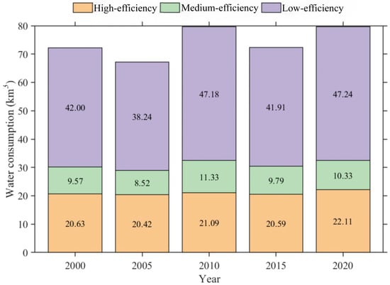
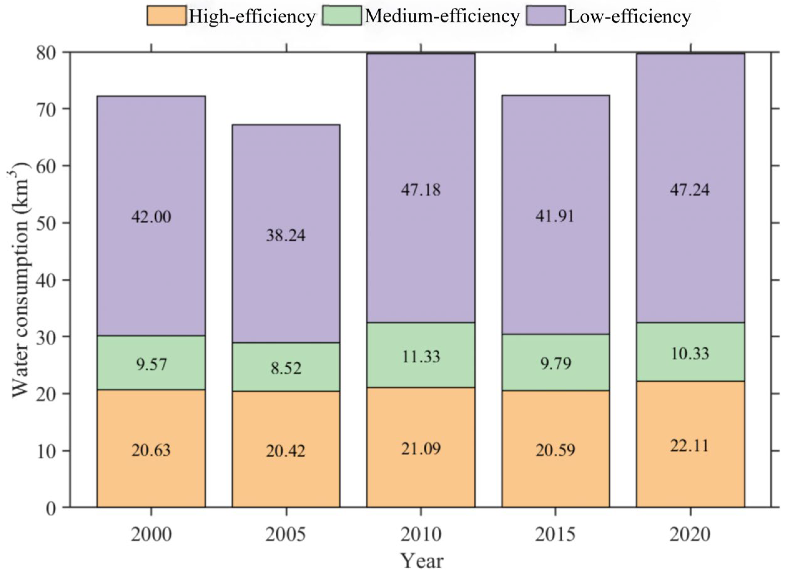
From 2000 to 2020, evapotranspiration water consumption in the Aksu River Basin irrigation districts showed a sustained upward trend (Table 6). Annual evapotranspiration increased at a rate of 2.83 mm/a, corresponding to an evapotranspiration water consumption growth rate of 0.33 × 10⁸ m3/a. Significant variations exist in the multi-year average evapotranspiration water consumption across different irrigation districts: Kuhe Irrigation District: 3.50 × 10⁸ m3 with an annual growth rate of 0.049 × 10⁸ m3/a; Tohu Wensu Irrigation District: 1.52 × 10⁸ m3 with an annual growth rate of 0.030 × 10⁸ m3/a. The Tarim River Irrigation District has a volume of 1.46 × 10⁸ m3 with an annual growth rate of 0.018 × 10⁸ m3/a. Evaluation results on irrigation water use efficiency indicate that the multi-year average total water consumption across the Aksu River Basin irrigation districts is 7.419 billion m3 (Figure 11), comprising inefficient water use (4.331 billion m3), efficient water use (2.097 billion m3), and moderately efficient water use (0.991 billion m3), accounting for 58.38%, 28.26%, and 13.36%, respectively. The inter-annual trends for all three water consumption categories align with the overall water consumption trend in the irrigation district, exhibiting annual growth rates of 0.28 billion m3/a, 0.06 billion m3/a, and 0.05 billion m3/a, respectively. Overall, inefficient water consumption dominates the water consumption structure in the Aksu River Basin irrigation district, with its inter-annual growth rate being the most pronounced among all efficiency categories.
Table 6.
Multi-year average water consumption of the five major irrigation districts in the Aksu River Basin.
Figure 11.
Evaluation results of water use efficiency in the Aksu River Basin irrigation district.
5. Discussion
Analyses of water consumption characteristics and water use efficiency in arid inland river basins critically depend on reliable and internally consistent estimates of actual evapotranspiration (ETa), which links regional water cycling with surface energy exchange. In this study, water use efficiency refers to a land use-based structural differentiation of water consumption at the basin scale rather than a ratio-based ecohydrological efficiency metric or a process-level partitioning between transpiration and evaporation. Uncertainty in ETa directly affects the interpretation of water consumption structures and the assessment of water use efficiency [37]. In arid and semi-arid regions, where precipitation is limited and evapotranspiration dominates the water balance, even modest ETa uncertainty may propagate through subsequent hydrological analyses [5,38]. Moreover, heterogeneous land surface conditions and strong human disturbances further complicate the representation of actual water consumption processes by any single model, particularly in inland river basins [39].
From a methodological perspective, Penman–Monteith (P–M)-based physical models exhibit strong theoretical consistency at point scales and are widely recommended by the FAO [40]. However, their sensitivity to meteorological inputs and surface parameters may limit robustness when extrapolated to basin scales. Remote sensing-based approaches enable spatially explicit regional analysis [41,42] but remain affected by model assumptions, parameter uncertainty, cloud contamination, and resolution constraints, which may introduce systematic biases in arid environments [43]. Water balance and complementary methods effectively capture long-term basin-scale variability but are less capable of resolving monthly dynamics and spatial heterogeneity [44,45]. Collectively, these studies indicate that ETa estimates vary across methods, with uncertainty conditioned by model structure and spatial scale.
Against this background, multi-source data integration and multi-model fusion have emerged as practical strategies for reducing model-dependent uncertainty and enhancing robustness. Previous research shows that ensemble-based approaches can mitigate systematic biases associated with individual models and improve the stability of spatiotemporal ETa series [8,13,46]. Building on these efforts, this study applies Bayesian Model Averaging (BMA) to integrate ETa estimates from diverse sources. By weighting model contributions using posterior probabilities, BMA avoids subjective weighting schemes and statistically exploits complementary information from physical models, remote sensing products, and reanalysis datasets, consistent with advances in hydrological ensemble modeling [3,47].
For the Aksu River Basin, where evapotranspiration dominates water consumption processes, the integrated ETa results exhibit improved spatiotemporal continuity and basin-scale consistency while maintaining physical plausibility. The magnitude and increasing trend of basin-scale ETa indicate sustained intensification during the study period. This increase is statistically consistent with regional climatic variability and documented expansion of irrigated agriculture; however, the present study does not conduct formal attribution analysis to quantify the relative contributions of climatic and anthropogenic drivers. These factors are therefore discussed as plausible contextual explanations rather than as confirmed causal mechanisms.
Regional warming may enhance atmospheric evaporative demand, while agricultural expansion and intensified irrigation practices are likely associated with increased land surface water consumption within managed oasis systems. Compared with climate-dominated ETa increases reported for less-managed arid basins, the relatively higher growth rate observed here may be associated with combined land use change and irrigation development in oasis-dominated environments. Nevertheless, these interpretations remain associative rather than causal.
Relative to previous single-source ETa estimates for the Aksu and broader Tarim River Basin, the present study reveals generally consistent spatial patterns but slightly higher basin-average ETa values. These differences are likely associated with explicit representation of irrigation-driven evapotranspiration and the multi-source fusion framework, which reduces systematic underestimation inherent in individual datasets [14,48]. Inter-annual variability in land use-specific ETa (Table 3) demonstrates that the relative ranking among land use types remains stable across benchmark years, indicating that the observed contrasts primarily reflect persistent surface characteristics rather than isolated annual anomalies.
Several limitations should be acknowledged. Because true basin-scale ETa observations are unavailable, the BMA-derived ETa should be interpreted as an ensemble-consistent estimate rather than a calibration against measured truth. The limited number of meteorological stations constrains the representation of fine-scale climatic heterogeneity, and spatial interpolation introduces uncertainty in local ETa patterns. However, because interpolation is used solely for descriptive visualization and does not serve as input for subsequent modeling or inference, residual interpolation uncertainty is unlikely to alter basin-scale gradients or long-term contrasts emphasized in this study.
Additional uncertainty arises from scale mismatch among MODIS, GLDAS, and GRACE datasets, which primarily affects local variability rather than basin-scale means or long-term trends. At monthly timescales, GRACE-based water balance ET may contain residual noise due to signal smoothing, leakage correction, unresolved boundary fluxes, and anthropogenic regulation; thus, GRACE-derived ET serves as a large-scale water balance constraint rather than an exact monthly estimate [49,50]. Validation, therefore, emphasizes temporal coherence, seasonal structure, and trend consistency rather than strict magnitude agreement under scale-mismatch conditions. Because BMA represents a convex combination of ensemble members and all ET products exhibit consistent inter-annual trend directions, moderate variation in weight magnitude would not alter long-term trend signs or dominant spatial contrasts. The ensemble fusion is therefore structurally stable with respect to the reference specification.
Despite these limitations, the main conclusions are supported by consistent long-term trends and spatial contrasts across independent ETa products, as well as their correspondence with regional climate conditions, topography, land use patterns, and irrigation gradients. Because the analysis focuses on statistical consistency and multi-source integration rather than process-based driver quantification, explicit attribution of ETa changes to specific climatic or anthropogenic factors remains beyond the scope of this study. Future research integrating ETa trends with temperature trajectories, precipitation variability, irrigation statistics, and vegetation dynamics would enable more rigorous attribution analysis. Under current data availability, the adopted framework provides a practical and scientifically defensible basis for evaluating evapotranspiration dynamics and water use efficiency in arid inland river basins.
6. Conclusions
Overall, the conclusions of this study are supported by multi-source evapotranspiration estimates and associated spatiotemporal and land use analyses, addressing the central research question concerning evapotranspiration dynamics and basin-scale water consumption structure in the Aksu River Basin.
This study developed an integrated framework for estimating actual evapotranspiration (ETa) at the basin scale using multi-source datasets and Bayesian Model Averaging (BMA). The framework provides spatiotemporally continuous ETa estimates at monthly, seasonal, and annual scales across the basin. The results indicate that the multi-year mean ETa during 2000–2020 was 290.93 mm, with pronounced inter-annual variability and a significant increasing trend of 4.04 mm/a. Intra-annual ETa exhibited a unimodal seasonal pattern, peaking in July–August and reaching minima in January and December. Spatially, ETa displayed a distinct “higher in the northwest and lower in the southeast” pattern, with higher values concentrated in forested mountainous areas and cultivated plains with greater vegetation cover, and lower values primarily distributed in desert foothills and oasis–desert transition zones.
Evaluation of water use efficiency based on land use-specific ETa differentiation indicated that ETa followed the order: grassland > cropland > forest land > unutilized land. The basin-wide multi-year average total water consumption reached 9.33 × 10⁹ m3, with low-efficiency water use accounting for 61.24%, exceeding the proportions of high-efficiency (26.01%) and medium-efficiency (12.75%) components. These results demonstrate that basin-scale water consumption is structurally dominated by land use types associated with lower vegetation-related water use intensity.
Overall, the Aksu River Basin is characterized by increasing evapotranspiration and a stable water consumption structure with pronounced land use differentiation. The findings highlight the importance of considering land use configuration and basin-scale water consumption structure in regional water resource planning. Under the current analytical framework, the results provide a structural and statistically consistent basis for evaluating evapotranspiration dynamics and water use efficiency in arid inland river basins.
Author Contributions
M.Y. performed the data analyses and wrote the manuscript; G.W. and S.Y. contributed to the conception of the study and the acquisition of funds; X.Y. helped perform the analyses via constructive discussions. All authors have read and agreed to the published version of the manuscript.
Funding
This research was supported by the National Scientific Foundation of China (NSFC) (no. U2003204, no. 52579015), the State’s Key Project of Research and Development Plan (2023YFC3206804), and the Scientific Research Project of the Tarim River Basin Management Bureau (TGJGLJJG-2024KYXM0003).
Data Availability Statement
The data supporting the findings of this study were derived from publicly available datasets. The sources and access details are as follows: MODIS data were obtained from the National Aeronautics and Space Administration (NASA) Earthdata portal (https://search.earthdata.nasa.gov/). GRACE terrestrial water storage data were acquired from NASA’s GRACE mission website (http://grace.jpl.nasa.gov). GLDAS evapotranspiration data were provided by NASA’s Global Land Data Assimilation System (https://ldas.gsfc.nasa.gov/gldas/). Digital Elevation Model (DEM) data were sourced from the Geospatial Data Cloud (GDC), China (http://www.gscloud.cn/). Meteorological data (temperature and precipitation) were obtained from the China Meteorological Science Data Center (http://data.cma.cn). Land use data were provided by the Resources and Environmental Science Data Center (RESDC), Chinese Academy of Sciences (http://www.resdc.cn/). The ERA5 reanalysis dataset was provided by the European Centre for Medium-Range Weather Forecasts (ECMWF) (https://cds.climate.copernicus.eu/datasets, accessed on 23 February 2026).
Acknowledgments
We thank the editors and anonymous reviewers for their useful suggestions and comments for improving this article.
Conflicts of Interest
The authors declare no conflict of interest.
References
- Liu, Y.; Yue, Q.; Wang, Q.; Yu, J.; Zheng, Y.; Yao, X.; Xu, S. A framework for actual evapotranspiration assessment and projection based on meteorological, vegetation and hydrological remote sensing products. Remote Sens. 2021, 13, 3643. [Google Scholar] [CrossRef] [Scilit]
- Wang, X.; Yao, Y.; Ren, S.; Shi, X. A Coupled FLUS and Markov approach to simulate the spatial pattern of land use in rapidly developing cities. J. Geo-Inf. Sci. 2022, 24, 100–113. [Google Scholar] [CrossRef]
- Wang, W.; Li, J.; Wei, J.; Shao, Q.; Deng, C.; Yu, Z. Runoff simulation by hydrological model based on the assimilated evapotranspiration. Adv. Water Sci. 2018, 29, 159–168. [Google Scholar] [CrossRef]
- Ye, L.; Lu, H.; Qin, S.; Zhang, L.; Xiong, L.; Liu, P.; Xia, J.; Cheng, L. Changes in pan evaporation and actual evapotranspiration of the Yangtze River basin during 1960–2019. Adv. Water Sci. 2022, 33, 718–729. [Google Scholar] [CrossRef]
- Pan, S.; Pan, N.; Tian, H.; Friedlingstein, P.; Sitch, S.; Shi, H.; Arora, V.K.; Haverd, V.; Jain, A.K.; Kato, E.; et al. Evaluation of global terrestrial evapotranspiration using state-of-the-art approaches in remote sensing, machine learning and land surface modeling. Hydrol. Earth Syst. Sci. 2020, 24, 1485–1509. [Google Scholar] [CrossRef] [Scilit]
- Yao, J.; Chen, Q.H.; Li, Q.F.; Cui, G.; Zhang, L.J. Spatial and temporal variability of evapotranspiration and influencing factors in the Ili River-Balkhash Lake Basin. Arid Zone Res. 2022, 39, 1564–1575. [Google Scholar] [CrossRef]
- Deng, H.; Lu, Y.; Wang, Y.; Chen, X.; Liu, Q. Assessment of actual evapotranspiration in the Minjiang River Basin Based on the GLDAS-Noah model. J. Geogr. Sci. 2022, 42, 548–556. [Google Scholar] [CrossRef]
- Wei, L.; Duan, K.; Liu, X.; Lin, Y.; Chen, X.; Wang, X. Assessing human-induced evapotranspiration change based on multi-source data and Bayesian model averaging at the basin scale. Shuili Xuebao 2022, 53, 433–444. [Google Scholar]
- Liang, W.; Yin, H.; Han, Z. Temporal and spatial variation analysis of evapotranspiration in Tabu river basin based on remote sensing. J. Inn. Mong. Agric. Univ. (Nat. Sci. Ed.) 2021, 42, 1–11. [Google Scholar]
- Bhattarai, N.; Wagle, P. Recent Advances in Remote Sensing of Evapotranspiration. Remote Sens. 2021, 13, 4260. [Google Scholar] [CrossRef] [Scilit]
- Zhang, Y.; Jia, Z.Z.; Liu, S.M.; Xu, Z.W.; Xu, T.R.; Yao, Y.J.; Ma, Y.F.; Song, L.S.; Li, X.; Hu, X.; et al. Advances in validation of remotely sensed land surface evapotranspiration. J. Remote Sens. 2020, 24, 975–999. [Google Scholar] [CrossRef] [Scilit]
- Zhang, W.F.; Su, T.; Lei, B.; Wang, L.; Sun, H.R.; Xu, Y.Y. Analysis of actual evapotranspiration during crop growth period in Chahanaoer watershed of Inner Mongolia based on multi-source data. Water Sav. Irrig./Jieshui Guan’gai 2021, 1–6. [Google Scholar]
- Yin, J.; Guo, S.; Wang, J.; Zhu, Q.; Zeng, Q.; Liu, H. Blending multi-source data in hydrological simulations based on BMA method. J. Hydraul. Eng. 2020, 51, 1335–1346. [Google Scholar] [CrossRef]
- Wang, Z.; Jiang, J.; Fang, G.; Chen, Z.; Cai, M.; Li, W. Analysis on the suitable scale of the Aksu Oasis under the limit of water resources. J. Glaciol. Geocryol. 2019, 41, 986–992. [Google Scholar] [CrossRef]
- Yao, X.; Gao, F.; Hang, F.; He, B. Land use intensity change and its influence on evapotranspiration in Aksu River Basin from 2000 to 2020. Arid Zone Res. 2024, 41, 951–963. [Google Scholar] [CrossRef]
- Bejagam, V.; Singh, A.; Sharma, A. Spatiotemporal variability and controlling factors of ecosystem water use efficiency in India. Theor. Appl. Climatol. 2023, 152, 813–827. [Google Scholar] [CrossRef] [Scilit]
- Bai, L.; Chen, Z.; Wang, C. Multi-scale response of runoff to climate change in the Aksu River Basin in Arid Area of the Northwestern China. Sci. Geogr. Sin. 2017, 37, 799–806. [Google Scholar] [CrossRef]
- Han, F.; Gao, F.; Wang, H.; He, B.; Liu, K. Effectiveness evaluation of water system connectivity of ecological water network in Aksu River basin based on graph theory. South-North Water Transf. Water Sci. Technol. 2025, 23, 1090–1099. [Google Scholar] [CrossRef]
- Penman, H.L. Natural Evaporation From Open Water, Bare Soil and Grass. Proc. R. Soc. Lond. Ser. A Math. Phys. Sci. 1948, 193, 120–145. [Google Scholar] [CrossRef] [Scilit]
- Li, S.; Feng, C.; Yang, L. Spatiotemporal patterns of evapotranspiration in the Xiangjiang River Basin from 2000 to 2020. Hydrol. Res. 2023, 54, 924–944. [Google Scholar] [CrossRef] [Scilit]
- Mu, Q.; Zhao, M.; Running, S.W. Improvements to a MODIS global terrestrial evapotranspiration algorithm. Remote Sens. Environ. 2011, 115, 1781–1800. [Google Scholar] [CrossRef] [Scilit]
- Yuan, L.; Chen, X.; Ma, Y.; Han, C.; Wang, B.; Ma, W. Long-term monthly 0.05° terrestrial evapotranspiration dataset (1982–2018) for the Tibetan Plateau. Earth Syst. Sci. Data 2024, 16, 775–801. [Google Scholar] [CrossRef] [Scilit]
- Liu, H.; Song, D.; Kong, J.; Mu, Z.; Zhang, Q.; Wang, X. Spatiotemporal Variation in Actual Evapotranspiration and the Influencing Factors in Ningxia from 2001 to 2020. Int. J. Environ. Res. Public Health 2022, 19, 12693. [Google Scholar] [CrossRef] [Scilit]
- Saxe, S.; Farmer, W.; Driscoll, J.; Hogue, T.S. Implications of model selection: A comparison of publicly available, conterminous US-extent hydrologic component estimates. Hydrol. Earth Syst. Sci. 2021, 25, 1529–1568. [Google Scholar] [CrossRef] [Scilit]
- Akl, M.; Thomas, B.F. Challenges in applying water budget framework for estimating groundwater storage changes from GRACE observations. J. Hydrol. 2024, 639, 131600. [Google Scholar] [CrossRef] [Scilit]
- Scanlon, B.R.; Zhang, Z.; Save, H.; Wiese, D.N.; Landerer, F.W.; Long, D.; Longuevergne, L.; Chen, J. Global evaluation of new GRACE mascon products for hydrologic applications. Water Resour. Res. 2016, 52, 9412–9429. [Google Scholar] [CrossRef] [Scilit]
- Huo, W.; Li, Z.; Li, Q. Hydrological models comparison and ensemble forecasting in semi-humid watersheds. J. Lake Sci. 2017, 29, 1491–1501. [Google Scholar] [CrossRef] [Scilit]
- Paradiso, S.; McGee, G.; Percival, W.J. Evaluating extensions to LCDM: An application of Bayesian model averaging and selection. J. Cosmol. Astropart. Phys. 2024, 2024, 021. [Google Scholar] [CrossRef] [Scilit]
- Seong, Y.; Choi, C.K.; Jung, Y. Assessment of uncertainty in grid-based rainfall-runoff model based on formal and informal likelihood measures. Water 2022, 14, 2210. [Google Scholar] [CrossRef] [Scilit]
- Mohyuddin, G.; Khan, M.A.; Haseeb, A.; Mahpara, S.; Waseem, M.; Saleh, A.M. Evaluation of machine learning approaches for precision farming in smart agriculture system: A comprehensive review. IEEE Access 2024, 12, 60155–60184. [Google Scholar] [CrossRef] [Scilit]
- Zhou, T.; Wen, X.; Feng, Q.; Yu, H.; Xi, H. Bayesian model averaging ensemble approach for multi-time-ahead groundwater level prediction combining the GRACE, GLEAM, and GLDAS data in arid areas. Remote Sens. 2022, 15, 188. [Google Scholar] [CrossRef] [Scilit]
- Sen, P.K. Estimates of the regression coefficient based on Kendall’s tau. J. Am. Stat. Assoc. 1968, 63, 1379–1389. [Google Scholar] [CrossRef]
- Li, C.; Yang, Z.; Wang, X. Trends of annual natural runoff in the Yellow River basin. Water Int. 2004, 29, 447–454. [Google Scholar] [CrossRef] [Scilit]
- Akl, M.; Thomas, B.F.; Clarke, P.J. A multi-objective comparative framework for Enhanced GRACE-Groundwater comparative analysis. J. Hydrol. 2025, 664, 134403. [Google Scholar] [CrossRef] [Scilit]
- Hirsch, R.M.; Slack, J.R.; Smith, R.A. Techniques of trend analysis for monthly water quality data. Water Resour. Res. 1982, 18, 107–121. [Google Scholar] [CrossRef] [Scilit]
- Wang, H.; Yang, G.; Jia, Y.W.; Qin, D.Y. Study on consumption efficiency of soil water resources in the Yellow River Basin based on regional ET structure. Sci. China Ser. D-Earth Sci. 2008, 51, 456–468. [Google Scholar] [CrossRef] [Scilit]
- Tran, B.N.; Van Der Kwast, J.; Seyoum, S.; Uijlenhoet, R.; Jewitt, G.; Mul, M. Uncertainty assessment of satellite remote-sensing-based evapotranspiration estimates: A systematic review of methods and gaps. Hydrol. Earth Syst. Sci. 2023, 27, 4505–4528. [Google Scholar] [CrossRef] [Scilit]
- Fisher, J.B.; Melton, F.; Middleton, E.; Hain, C.; Anderson, M.; Allen, R.; McCabe, M.F.; Hook, F.; Baldocchi, D.; Townsend, P.A.; et al. The future of evapotranspiration: Global requirements for ecosystem functioning, carbon and climate feedbacks, agricultural management, and water resources. Water Resour. Res. 2017, 53, 2618–2626. [Google Scholar] [CrossRef] [Scilit]
- Li, X.; Yu, D. Progress on evapotranspiration estimation methods and driving forces in arid and semiarid regions. Arid Zone Res. 2020, 37, 26–36. [Google Scholar]
- Allen, R.G.; Tasumi, M.; Trezza, R. Satellite-based energy balance for mapping evapotranspiration with internalized calibration (METRIC)—Model. J. Irrig. Drain. Eng. 2007, 133, 380–394. [Google Scholar] [CrossRef] [Scilit]
- Zhou, J.; Cheng, G.; Li, X. Application of remote sensing technology to estimate river basin evapotranspiration. J. Hydraul. Eng. 2009, 40, 679–687. [Google Scholar]
- Tang, R.; Wang, S.; Jiang, Y. A review of retrieval of land surface evapotranspiration based on remotely sensed surface temperature versus vegetation index triangular/trapezoidal characteristic space. Natl. Remote Sens. Bull. 2021, 25, 65–82. [Google Scholar] [CrossRef] [Scilit]
- Sun, S.K.; Li, C.; Wang, Y.B.; Zhao, X.N.; Wu, P.T. Evaluation of the mechanisms and performances of major satellite-based evapotranspiration models in Northwest China. Agric. For. Meteorol. 2020, 291, 108056. [Google Scholar] [CrossRef] [Scilit]
- Jian, D.; Li, X.; Tao, H.; Huang, J.; Su, B. Spatio-temporal variation of actual evapotranspiration and its influence factors in the Tarim River basin based on the complementary relationship approach. J. Glaciol. Geocryol. 2016, 38, 750–760. [Google Scholar]
- Jiang, X.M.; Wang, G.Q.; Xue, B.L.; Yao, J.P. Spatiotemporal variations and driving forces of actual evapotranspiration in Hunhe River basin based on Budyko theory and complementary model. Chin. J. Ecol. 2022, 41, 1361. [Google Scholar] [CrossRef]
- Ezenne, G.I.; Eyibio, N.U.; Tanner, J.L.; Asoiro, F.U.; Obalum, S.E. An overview of uncertainties in evapotranspiration estimation techniques. J. Agrometeorol. 2023, 25, 173–182. [Google Scholar] [CrossRef] [Scilit]
- Moriasi, N.D.; Arnold, G.J.; Van Liew, M.W.; Bingner, R.L.; Harmel, R.D.; Veith, T.L. Model Evaluation Guidelines for Systematic Quantification of Accuracy in Watershed Simulations. Trans. ASABE 2007, 50, 885–900. [Google Scholar] [CrossRef] [Scilit]
- Yang, P.; Xia, J.; Zhan, C.; Mo, X.; Chen, X.; Hu, S.; Chen, J. Estimation of Water Consumption for Ecosystems Based on Vegetation Interfaces Processes Model: A Case Study of the Aksu River Basin, Northwest China. Sci. Total Environ. 2018, 1, 185–195. [Google Scholar] [CrossRef] [Scilit]
- Vinukollu, R.K.; Meynadier, R.; Sheffield, J.; Wood, E.F. Multi-model, multi-sensor estimates of global evapotranspiration: Climatology, uncertainties and trends. Hydrol. Process. 2011, 25, 3993–4010. [Google Scholar] [CrossRef] [Scilit]
- Kim, D.; Lim, Y.; Kang, M.; Choi, M. Land response to atmosphere at different resolutions in the common land model over East Asia. Adv. Atmos. Sci. 2016, 33, 391–408. [Google Scholar] [CrossRef] [Scilit]

Disclaimer/Publisher’s Note: The statements, opinions and data contained in all publications are solely those of the individual author(s) and contributor(s) and not of MDPI and/or the editor(s). MDPI and/or the editor(s) disclaim responsibility for any injury to people or property resulting from any ideas, methods, instructions or products referred to in the content. |
© 2026 by the authors. Licensee MDPI, Basel, Switzerland. This article is an open access article distributed under the terms and conditions of the Creative Commons Attribution (CC BY) license.