


Abstract
While global decarbonization and low-temperature engines curb nitrogen oxides, they risk significant N2O emissions, which is also one of the greenhouse gases. This review evaluates N2O monitoring strategies across maritime and industrial combustion environments. Furthermore, this paper provides a rigorous comparative assessment of analytical monitoring methodologies. We evaluate the adaptability of established agricultural techniques. In parallel, advanced spectroscopic and non-spectroscopic sensor technologies (DAS, NDIR, TDLAS, PAS, CRDS, CEAS, FTIR, GC, and electrochemical/chemiresistive sensors) are critically analyzed regarding their sensitivity, response time, cross-interference vulnerabilities, and suitability for harsh industrial stacks and maritime settings. Finally, the levels of N2O above background from individual sources are estimated using wind-tunnel modeling studies. Emissions from ships, truck lines, and industrial turbines typically cause urban ambient concentrations ranging from hundreds down to tens of ppb, whereas individual trucks and rural ship levels are significantly lower, from below 1 ppb up to about 70 ppb depending on engine optimization. For industrial and combustion sources, real-time N2O analysis can be performed using FTIR, which allows for multi-gas mixture measurement, or TDLAS for targeted N2O detection. For distributed screening and monitoring around industrial plants, NDIR is a technically viable option under specific conditions. For mobile sources, TDLAS, FTIR, and highly sensitive cavity-enhanced methods (CRDS, CEAS) are suitable, provided they are optimized for harsh conditions. NDIR is applicable here only in dense urban areas. In all scenarios, gas chromatography can be used, though it requires physical sample collection and does not offer real-time analysis. As we will show, electrochemical and chemiresistive sensors cannot currently be used. Similarly, PAS is unsuitable for ambient enhancement detection, despite its applicability to stack sampling.
1. Introduction
Nitrous oxide (N2O) represents a less conspicuous, yet extremely dangerous greenhouse gas in the context of the current climate crisis. Its globally averaged atmospheric concentration was 339.9 ppb in June 2026 (NOAA global monthly mean), with an annual growth rate of 1.0–1.3 ppb per year in 2020–2025 according to the same source [1]; this long-term rise is driven mainly by anthropogenic emissions [2]. While global political and scientific efforts are currently focused primarily on reducing carbon dioxide (CO2) as the main culprit behind global warming, the specific properties of nitrous oxide often remain in the background of interest. However, in terms of its ability to trap heat in the atmosphere, N2O is a greenhouse gas with a 100-year global warming potential (GWP100) of 273 relative to CO2 [3], which makes it a critical threat to climate stability [2,4]. Paradoxically, the risk of its massive release into the atmosphere increases as humanity attempts to transition to so-called carbon-free fuels.
1.1. Background and Problem Statement
One of the main pillars of this decarbonization is intended to be ammonia (NH3), considered an alternative fuel for energy and heavy transport [5,6,7]. However, if power plants or large cargo vessels in maritime transport were to switch to ammonia combustion, we encounter a fundamental technological limit: the process of incomplete combustion. During this process, nitrous oxide is produced as an undesirable byproduct [8,9]. If there is a failure to optimize combustion processes on such a massive scale, there is a risk that we will merely replace CO2 emissions with a gas that is carbon-free but climatically much more destructive.
The automotive industry is dealing with a similar technological contradiction. In an effort to meet strict limits for toxic nitrogen oxides (NOx), low-temperature combustion has begun to be used in modern engines [10,11]. Although this method successfully reduces the concentration of health-harmful NOx in exhaust gases, lower temperatures in the reaction zone create ideal conditions for the unwanted synthesis of stable nitrous oxide. This problem could deepen dramatically in the future, as there is consideration of introducing ammonia combustion for trucks as well [12]. Finding a balance between eliminating local toxicity (NOx) and the global ecological footprint (N2O) is thus becoming one of the greatest challenges for contemporary engine engineering.
1.2. Objective of the Review
The primary objective of this paper is to conduct a comprehensive review of the current technological landscape regarding nitrous oxide monitoring, while specifically addressing the critical gap between existing sensor reviews and real-world industrial and maritime requirements. While general overviews of gas-sensing technologies or agricultural N2O measurements are widely available in the literature, this study distinctly moves beyond purely instrumental descriptions by directly linking analytical capabilities with specific emission scenarios anticipated in the transition toward carbon-free fuels—particularly ammonia combustion in maritime shipping, industry, and heavy-duty transport. By integrating atmospheric dispersion modeling, this paper bridges the gap between source emission rates and ground-level ambient concentrations, providing a practical framework for identifying localized emission ‘hotspots’ that necessitate targeted ground-based monitoring solutions. Consequently, satellite-based remote sensing falls outside the scope of this work, as our focus remains strictly on localized, actionable compliance and emission control.
1.3. Review Methodology
The study adopts a semi-systematic review approach. The review is based on peer-reviewed scientific studies and data indexed in major international academic databases:
- Scopus and Web of Science (for comprehensive multidisciplinary coverage of peer-reviewed journals).
- Google Scholar (for tracking the grey literature, conference proceedings, and broader academic outputs).
The search strategy relied on specific combinations of measurement techniques, emission sources, and target gases to capture relevant data. The literature was carefully chosen to directly connect the analytical performance of sensors—such as detection limits, response time, and cross-interference—with real-world emission scenarios. The selected sources range from foundational historical milestones to cutting-edge contemporary studies and official reports published up to 2026.
(Note: Throughout this review, ppm and ppb denote mole fractions (µmol mol−1 and nmol mol−1, respectively); values reported as ppmv or ppbv in the cited studies are equivalent and are given here as ppm or ppb.)
The remainder of the paper is structured as follows: Section 2 provides information about N2O formation and combustion hotspots. Section 3 contains a critical overview of current methods employed in agricultural contexts. Section 4 presents an analysis of available sensor technologies suitable for N2O detection. Subsequently, the discussion contains a comparative assessment of sensor technologies, then evaluates characteristic emission levels in various scenarios and identifies the most promising monitoring strategies tailored to the identified industrial needs. Finally, the concluding section synthesizes our main findings and offers perspectives on future research directions in this critical area.
2. N2O Formation, Climate-Relevant Thresholds, and Source-Term Implications for Ammonia Combustion Hotspots
Nitrous oxide formation during ammonia combustion is governed primarily by the homogeneous gas-phase reaction NH + NO ↔ N2O + H, whereas its destruction proceeds mainly through N2O + H ↔ N2 + OH and the third-body dissociation pathway N2O(+M) ↔ N2 + O(+M) [13,14,15,16]. However, numerical analysis of the oxidation of ammonia and methane mixtures in an idealized (plug-flow) reactor shows that at relatively low temperatures below 1300 K, N2O is produced mainly through the reaction of NH2 with NO2, as represented by NH2 + NO2 ↔ N2O + H2O [16,17,18,19].
Mechanistic chemical kinetic studies (usually assuming idealized reactors and laminar flames) are indispensable because they identify the dominant chemistry and confirm that N2O is favored in cooler, ammonia-rich regions, while hotter zones promote its decomposition [18,19]. However, these studies can underrepresent practical emissions because real combustors contain turbulent recirculation, cold-wall effects, local quenching, and nonuniform mixing. This is consistent with experimental swirl-burner data, where N2O remained modest at lower ammonia shares but rose sharply above about 80 vol.% NH3, reaching hundreds to thousands of ppm [18], whereas a pure NH3 flame could still produce around 240 ppm N2O with a global warming effect comparable to the CO2 from an equivalent methane flame [20].
Across nitrogen-containing fuels including ammonia, the highest N2O formation is generally associated with intermediate temperatures (800–1200 K), while above roughly 1200 K thermal decomposition becomes dominant [15]; this makes post-flame cooling, wall heat loss, and residence time central control variables for ammonia systems [21,22].
Bertagni et al. [23], whose study serves as the key reference for the thresholds used in this review, estimated that the ammonia economy would have the same climate impact as the fossil-fuel energy system (the “climate-parity threshold”) in the case of a 0.4% nitrogen conversion from NH3 to N2O when considering only emissions from the combustion devices themselves, without considering all upstream emissions related to ammonia production. Their estimate is based on GWP-100 = 265 and an NH3 lower heating value (LHV) of 19 GJ/t.
The literature becomes ambiguous as soon as such a threshold is translated into engineering units, because authors alternate among %N-to-N2O conversion, ppm, g/kg fuel, g/kWh (of fuel energy or of output), g/MJ, and, in some cases, indirect nitrogen-to-N2O conversion in the environment rather than direct combustion emissions. A second ambiguity is methodological: older and newer studies do not use the same 100-year GWP for N2O, with values of 298, 265 (used by Bertagni et al. [23]), and 273, all appearing in current practice depending on whether AR4, AR5, or AR6 conventions are followed.
To avoid these ambiguities, this review uses the AR6 values GWP-100 = 273 ± 130 and LHV = 18.6 MJ/kg, which were calculated from the Active Thermochemical Tables (ATcT). This changes the parity threshold of Bertagni et al. by only about 5% (to 0.38%), well within the uncertainty of GWP-100 (a range of ≈ 0.3–0.8%); it is therefore retained as the original value, i.e., 0.4%, for the sake of simplicity and consistency. A similar value was obtained independently by Wolfram et al. for the shipping sector (about 1 g N2O per kWh of NH3 fuel energy, with GWP-100 = 298 and LHV = 18.8 MJ/kg). In energy-based units, 0.4% corresponds to 0.28 g N2O per MJ of NH3 fuel energy (1.0 g/kWh of fuel energy), i.e., about 1.7 g/kWh of output at 60% (electrical conversion) and about 2.5 g/kWh at 40% (engine-like) efficiency, respectively (Table 1).
Table 1.
Conversion of the N2O climate-parity threshold to engineering units: GWP version, NH3 lower heating value, and efficiency assumed for each value.
A further caveat is physical rather than accounting-based, because laminar or low-dimensional kinetic studies isolate chemistry, whereas turbulent combustors introduce wall quenching, mixing inhomogeneity, and broader residence-time distributions that can strongly amplify device-scale N2O relative to idealized flames.
In addition to the direct N2O released at the point of combustion itself, ammonia use as a fuel carries a second, indirect emission pathway: unburnt NH3 and NOx that escape the combustor are deposited on land and in water, where soil and aquatic microorganisms responsible for the natural nitrogen cycle convert part of this deposited reactive nitrogen into secondary N2O, distinct from and additive to what is measured directly at the stack or exhaust. For ammonia combustion systems, this cascade effect means that monitoring and regulating only tailpipe/stack N2O captures only part of the true climate and ozone-depletion footprint of the fuel’s nitrogen chemistry. This matters because other authors express the same underlying concern in different terms: Esquivel-Elizondo et al. [25] report that combustion emissions above 0.28 g/MJ, equivalent to about 1 g/kWh of fuel energy, would by themselves nearly match the well-to-wake greenhouse-gas intensity of conventional marine fuels. The same value has been considered in the specific analysis of shipping emissions [24].
It is worth noting that beyond its greenhouse effect, once N2O reaches the stratosphere, it is broken down by ultraviolet radiation, forming NOx as byproducts that catalytically deplete stratospheric ozone. Global N2O emissions are now considered the most significant remaining ozone-depleting emission source overall [23].
The gap appears in engines, where the literature consistently links higher ammonia energy share, partial-load operation, and delayed or incomplete combustion to higher N2O. A marine case summarized for IMO/MEPC (https://www.imo.org) reported 297 ppm N2O at 83% NH3 share, 75% load, and 1200 rpm, equivalent to roughly 1.5 g N2O per kg NH3 consumed. For ammonia–diesel dual-fuel engines, a recent review [26] reports N2O emissions of 0.1–3 g/kWh for low-pressure port injection (LPDF) and 0.5–10 g/kWh for high-pressure direct injection (HPDF) (Table 2). Optimized HPDF operation at an ammonia energy ratio (AER) of up to about 60% yields ≤ 0.1 g/kWh, far below the parity threshold of about 2.5 g/kWh (Table 1), and most data at intermediate AER lie between 0.4 and 1.5 g/kWh. At AER of 80–95%, however, the worst cases reach about 3–10 g/kWh, which exceeds the parity threshold by up to about fourfold, and the 1% high-loss case (≈6.3 g/kWh) by up to about 1.6-fold. For the same fuel pair, the best and worst operating points thus differ by more than two orders of magnitude. This confirms the key mechanistic pattern: N2O forms primarily in local low-temperature zones during incomplete combustion and flame quenching, rather than during stable, fully burned-out operation, and its control depends on injection strategy, airflow organization, and combustion-chamber design rather than on the choice of LPDF or HPDF [26]. This is a key finding for monitoring purposes, as it shows that N2O emissions are not a fixed property of “the NH3 engine” but depend strongly on the specific operating point—load, AER, and injection timing—which requires continuous, rather than one-off, monitoring under real-world operation to capture excursions into high-risk regimes.
Table 2.
Representative ranges of N2O emissions of ammonia–diesel dual-fuel engines for optimized and worst-case operation, compiled from [26] (values read from Figure 21 of [26], rounded), compared with the thresholds in Table 1 (η = 40%). The bounding cases are based on the primary studies of Nyongesa et al. [27] and Guo et al. [28] (optimized operation) and of Dong et al. [29], Cui et al. [30] and Zuo et al. [31] (worst case).
Regulatory benchmarks add a further layer to this picture, since the newly adopted Euro 7 standard introduces the first gravimetric N2O limit for heavy-duty vehicles, set at 0.200 g/kWh ~ (Regulation (EU) 2024/1257, Table 2) [34]. By contrast, Euro VI, in force until 2028, contained no N2O limit at all and regulated only NOx at 0.40 g/kWh, so the new ceiling is a direct response to the growing use of low-temperature combustion strategies and, prospectively, ammonia as a heavy-duty fuel, both of which generate N2O through the same NH + NO ↔ N2O + H pathway seen in marine and stationary combustion. When ammonia–diesel dual-fuel engines are evaluated against this benchmark rather than against conventional diesel baselines, a clear regime-dependent pattern emerges (Table 2): only the best HPDF cases (≤0.1 g/kWh) are comparable to conventional Euro V/VI diesel and CNG heavy-duty engines (about 0.045–0.15 g/kWh), whereas typical operation at intermediate AER (about 0.4–1.5 g/kWh) exceeds the Euro 7 limit severalfold while remaining below the parity threshold. At AER ≥ 80%, the worst cases exceed the Euro 7 limit by a factor of 15–50 and the parity threshold by a factor of 1.2–4. Yet this comparison also exposes a striking asymmetry: if heavy-duty NH3 trucks become subject to a 0.20 g N2O/kWh ceiling, marine engines, gas turbines, and industrial boilers burning NH3 currently face no comparable stack-level N2O limit or measurement requirement, even though these are exactly the sectors expected to carry the largest future volumes of ammonia fuel demand. For shipping, N2O is covered in the well-to-wake greenhouse-gas intensity of FuelEU Maritime [35] and the IMO 2024 LCA Guidelines [36], but through default emission factors and CO2-equivalent accounting rather than through measured emissions. As a result, the sectors with the greatest absolute N2O source-term potential remain the least regulated in terms of measured N2O emissions, which should directly shape how monitoring resources are prioritized across the ammonia value chain.
3. Ambient Methods and Flux
N2O was discovered in 1772, but its role as a greenhouse gas and its measurement in agricultural soils only became a major research focus in recent decades, as fertilizer use and climate concerns grew [37]. Initial methods covered simple soil chambers, which have been used since the 1970s. Since the 1990s, micrometeorology (flux-gradient, eddy covariance) methods have started to be used [38,39]. The measurements evolved using advanced lasers, FTIR, high-precision chambers or isotope techniques [40,41,42].
In this chapter, the common methods used in agriculture for N2O measurements are introduced. Moreover, we show if and how these methods could be used for N2O measurements coming from combustion processes. Special sensors (e.g., NDIR sensors, FTIR) as part of advanced measurement systems are discussed in the next separate chapter.
3.1. Chamber Methods
Traditionally, the low-cost solution for agricultural measurements is a static chamber method. This method allows for the increase of the small N2O signal for in situ measurements. The principle lies in enclosing a known surface area, typically a low metal cylinder enclosed with a cover. The sample is then taken by injection, and this sample is analyzed in a laboratory, e.g., by chromatography. The alternative is to connect the chamber to a photoacoustic analyzer; the air is recirculated between the analyzer and the instrument, and the increase in N2O concentration is measured once a defined time [43].
Static chambers, however, are unsuitable for combustion processes because the high flow rates and exhaust pressure would cause a dangerous pressure buildup or stifle the engine. They might be used to measure emissions at component levels (e.g., vents, leakages in tubes or specific small infrastructures). In this method, the static chamber is placed over a leaking component to create a seal. Such a method is described for methane measurements in [44].
3.2. Diffusion Tubes
The alternative could be diffusion tubes. They are, however, currently used for nitrogen dioxide, not nitrous oxide. They look like small tubes with a cap, under which is a steel mesh disc that is coated, e.g., with triethanolamine (TEA), a chemical that absorbs nitrogen dioxide. The tubes are placed in ambient air. They operate on the principle of molecular diffusion and do not require a pump; they are left on-site for several days to weeks, after which the average concentration of pollutants is analyzed in a laboratory [45]. Diffusion tubes are nowadays not used for nitrous oxide. This methodological gap could possibly be bridged in the future using materials and methods that are tested e.g., in indoor environments. For example, [46] developed a passive sampling method for the quantitative measurement of exposure to nitrous oxide for occupational exposure assessment. The passive sampler consists of a small glass tube filled with molecular sieve 5A. Nitrous oxide naturally diffuses into it from the surrounding air. After sampling, the tube is sealed in a vial and heated to 100 °C to achieve solid-gas equilibrium. The headspace air is subsequently analyzed using a gas chromatograph with an electron capture detector.
In contrast to static chambers, this method could be used for analyzing combustion processes. Researchers often employ a method where samplers are placed upwind of the farm to determine background levels and downwind to capture the emission plume; the difference in concentrations then indicates the total emissions contributed by the farm to the atmosphere. Hence, similarly, the tube might be placed in front of the factory in the prevailing wind direction or near the harbor and behind the factory/ in the harbor. The difference in N2O measurements between these two tubes would be the estimated N2O produced by the factory or ships in the harbor.
The disadvantage of this method lies in the measurement of only mean values over a chosen time. One cannot see peaks of emissions during the day. In the combustion problems, the harbor would not be able to distinguish whether the emissions of N2O from ships are more or less similar across all ships or whether a ship or a type of ship would be the origin of the majority of the seen pollution. Only a method enabling such a separation would enable harbor management to have the possibility, eventually, not to let in a ship with unsuitable emission parameters to their location.
An alternative would be to place the diffusion tubes on the individual ships themselves and have mandatory records of emissions from their voyage. The experiments with diffusion tubes on ships were up to date done with polyurethane foam passive samplers to measure PAHs in indoor occupational air for seafarers, before and after fuel changes, not for stack emissions [47]. Diffusion tubes give time-averaged concentrations at a point, with known biases near strong, fluctuating sources and in windy conditions. Translating such point concentrations into mass emissions from a moving source would require additional modeling [48,49,50]. Such methodology, however, always brings another uncertainty that could, in extreme cases, lead to unreliable results.
3.3. Eddy Covariance and Relaxed Eddy Accumulation Method
The Eddy Covariance method is based on the measurement of wind velocity and gas concentrations on a mast at various heights above the ground. This method needs fast-response laser instruments, tunable diode lasers–usually quantum cascade lasers—which have high sensitivity. Hence, this method is not low-cost. In contrast, the relaxed eddy covariance method does not use a fast-response analyzer. It collects air from up-drafts and down-drafts into separate reservoirs over a specified duration. The reservoirs are analysed by a slow response analyser enabling to estimate average fluxes [51].
This method belongs to the micrometeorological methods requiring homogeneous terrain, such as expansive open fields. It faces significant limitations in industrial or port environments. Because the method relies on high-frequency measurements (10–20 Hz) of vertical wind fluctuations, the mechanical turbulence and wake effects caused by buildings and cranes violate the fundamental physical assumptions of the method, leading to highly unreliable data in such complex terrains. However, corrections are used to be able to break these assumptions. At a coastal site influenced by ship emissions, the eddy covariance method was used to derive fluxes and fuel sulfur content, after correcting for flow distortion and wave effects [52]. Moreover, for large industrial or urban areas, tall-tower eddy covariance or the relaxed eddy covariance method can be used to capture aggregated emissions from multiple factories within the footprint [53,54,55].
3.4. Aerodynamic Gradient Method
The aerodynamic gradient method is based on measurements of vertical profiles of concentrations, wind and temperature. The wind and temperature measurements are used for the calculation of the eddy exchange coefficient obtained with the use of similarity theory. The flux is then obtained by multiplying the eddy exchange coefficient by the vertical concentration gradient.
This method also belongs to the micrometeorological type, requiring situations where air has passed over a homogeneous exchange surface for a sufficient distance, so profiles are in equilibrium with local exchange. It was used on a coastal mast in the Baltic Sea by a ship route to measure fluxes of various gases (but not N2O) and nanoparticle number, with ship traffic clearly affecting the measured fluxes and allowing evaluation of ship impacts, provided flow distortion by obstacles and waves is corrected (e.g., using mathematical modeling) [52]. So, in principle, this method can be applied near harbors or factories for N2O, but reliability depends on meeting micrometeorological assumptions (homogeneous, stationary flow) or correcting for disturbed wind fields and obstacles. Given these conditions, the method is applicable for industrial purposes only in special cases.
3.5. Micrometeorological Mass Balance Method
The principle of the micrometeorological mass balance method lies in concentration measurements at several heights on upwind and downwind boundaries, multiplied by horizontal wind to get horizontal flux profiles. Then the upwind–downwind differences are integrated to obtain the emission rate [55,56,57].
The method requires sufficient wind speed and relatively steady wind direction. Complex urban or building-induced flows can distort gradients. For the vertical measurements, towers, drones or aircraft are needed. The method is already used to measure N2O and CH4 emissions from defined area sources such as landfills or manure storage [55,58,59]. With suitable geometry, wind characterization, and instrumentation, the same principles could be applied to harbors and industrial facilities. However, applying this method to complex industrial areas or harbors introduces severe challenges due to dense infrastructure, multi-directional building-induced turbulence, and overlapping emission sources. Consequently, isolating a specific facility’s contribution in a dynamic industrial environment remains highly uncertain and technically demanding.
3.6. Plume Method
The plume method uses measurements and mathematical modeling in combination. The method requires knowledge of wind speed and direction as well as turbulent parameters. The concentrations are measured by sensors–e.g., opto-acoustic or gas chromatography (GC). The data are used as input parameters for a mathematical model. Traditionally, one can use a Gaussian model. The advantage of this method is its simplicity, the need for a relatively small amount of meteorological data, and that different operators get the same results. Its disadvantages are that it very often overestimates concentrations and assumes stationarity. The method does not work well in complex terrain, and the plume from the source is straight according to the prevailing wind direction. It cannot see obstacles and does not work well for positions very close to the gas source. A modern alternative is to use a backward Lagrangian model. This method, however, requires an expert, much more meteorological data as input, and different people can obtain different results. Hence, without standardization, such a method cannot be used for legislative purposes.
Plume methods—especially Gaussian plume models—are routinely used to estimate concentrations and emissions from factories and ships, including in harbors. They can, in principle, be applied to N2O just as they are to NOx, SO2, CO2 and other gases. Except for a straightforward usage of the method, some advanced approaches can be found in the literature. An improved Gaussian plume line-source model plus genetic algorithms was used to invert measured concentrations and estimate ship emission source intensity and even fuel sulfur content, with approx. 85% accuracy in identifying non-compliant vessels [60]. Long-path differential optical absorption spectroscopy (DOAS) measurements across a shipping lane, combined with a Gaussian plume model, enabled derivation of NOx and SO2 emission rates for individual ships without needing fuel-consumption data [61]. Reviews of port air-quality modeling highlight Gaussian plume/puff models as standard tools for assessing port emissions and supporting decision-making [62].
A special method is plume-intercept measurement. The method is used to measure real-world emissions from moving vehicles, ships, or aircraft without attaching equipment directly to their exhaust. A mobile station, drone, or roadside sensor passes through the exhaust plume to measure the ratio between a specific pollutant and CO2. Based on the known carbon content of the fuel, it calculates the exact emission factor (e.g., g/kg fuel or g/kWh) while operating under normal conditions [63].
4. N2O Sensors Technologies
4.1. Spectroscopy Techniques
4.1.1. Spectroscopic Fingerprints of N2O
N2O is a linear asymmetric molecule, which gives rise to a rich ro-vibrational spectrum. Nitrous oxide has many infrared absorption bands from near-IR to mid-IR. For gas sensing, most laser systems use strong mid-IR bands. However, other N2O bands also exist (Figure 1).
Figure 1.
N2O spectrum in the entire IR region. Redrawn based on data from the NIST Standard Reference Database 69 (NIST Chemistry WebBook, Source: NIST Standard Reference Database). (https://webbook.nist.gov/cgi/cbook.cgi?ID=C10024972&Type=IR-SPEC&Index=1#IR-SPEC (accessed on 6 November 2026)).
In the near-IR spectrum, N2O detection relies on weaker overtone and combination bands. The spectrum is characterized by a few windows, mostly within the region 1.74 to 0.83 µm [64,65,66]. Two notable spectral windows for these measurements include the 7250–7653 cm−1 (1.307–1.379 µm; [67]) and 8325–8622 cm−1 (1.16–1.20 µm; [66]) ranges. Bertin et al. [65] measured near 1.74 µm, Liu et al. [68] 1.56 µm, and Karlovets et al. [66] 1.18 µm. Due to the lower line intensities in these bands compared to the fundamental transitions, standard absorption spectroscopy lacks the necessary detection limits for trace-gas analysis. However, this limitation is effectively overcome by employing high-sensitivity methods such as Cavity Ring-Down Spectroscopy (CRDS; [69]). The primary driver for utilizing the near-IR region despite its weaker absorption features is technological: it aligns perfectly with the mature, highly stable, and cost-effective laser diodes and fiber-optic components developed for the telecommunications industry. This synergy enables the development of robust, field-deployable, and relatively inexpensive instruments capable of reaching parts-per-billion (ppb) sensitivity [70].
In the mid-IR spectrum, N2O can be detected in a few regions:
The 4.4–4.6 µm region (2180–2295 cm−1) is widely considered the gold standard for high-sensitivity, high-precision N2O monitoring. Because line intensities here are orders of magnitude higher than in the near-IR, this window is extensively targeted by sensors utilizing Quantum Cascade Lasers (QCLs) and Interband Cascade Lasers (ICLs) to achieve sub-ppb (parts-per-billion) detection limits (Shao et al. [71]—4.54 µm; Yang et al. [72]—4.56 µm). Furthermore, this region provides sufficient spectral resolution and line separation to distinguish between different N2O isotopologues (e.g.,14N15N16O, 15N14N16O, and 14N14N18O), which is vital for tracing agricultural and atmospheric source fingerprints [73].
The 3.9 and 4.5 µm are Lidar Windows [74,75]. For remote sensing and open-path atmospheric profiling, the focus shifts toward optimizing laser propagation through the atmosphere. Simulation and modeling studies have identified specific “lidar bands” around 4.5 µm and 3.9 µm (secondary option with tighter stability requirements) as optimal candidates for airborne Differential Absorption Lidar (DIAL) systems. These windows balance the requirement for strong N2O absorption features with the necessity of minimizing attenuation from background atmospheric gases, allowing for long-range vertical profiling of greenhouse gas distributions.
The 7.3–8.9 µm region [76] serves as a powerful fingerprint region for N2O. Prominent doublets located at 7.69 µm and 7.88 µm are frequently exploited. Beyond conventional absorption spectroscopy, this highly distinct spectral structure has recently found utility in advanced quantum optics, serving as a primary target in quantum interferometric spectroscopy and non-linear optical frequency conversion techniques.
Far infrared-Long-wave infrared spectrum is at the 17 µm region [77]. While technically more challenging due to detector cooling requirements and background thermal noise, this region features exceptionally narrow, well-isolated ro-vibrational lines. Consequently, rather than being used for standard environmental trace gas sensing, these transitions are primarily utilized as highly precise frequency references and calibration standards for laboratory spectroscopy.
4.1.2. Typical Sensor Architecture
Mostly absorption sensor for N2O follows the Beer–Lambert architecture (Figure 2): light from a source passes through a gas region (with various optical geometries used), and a detector measures the transmitted intensity to infer concentration [78,79,80]. The main architectural changes are in the source type, the wavelength-selection method, and the cell design rather than in the basic source–cell–detector logic [81,82,83].
Figure 2.
Typical sensor architecture. (Note: The authors declare that AI tools (ChatGPT) were used to assist in the generation and layout of this figure, in accordance with the journal’s AI policy.).
This architecture is different for the FTIR technique, in which an interferometer and Fourier transformation are used (see below).
4.1.3. Source Types
Two types of sensors–incoherent and coherent are used. Laser sources, which are coherent, dominate high-sensitivity N2O sensing, while LED and broadband thermal-style sources, the incoherent sources, are emerging for lower-cost, simpler, but generally less sensitive devices.
Incoherent Sources
- LED source
A mid-infrared LED source is a broadband, incoherent emitter in the spectral region where N2O has strong fundamental absorption bands, especially around 4.0–4.6 µm [84]. For N2O sensing, LEDs are studied because they can enable compact, low-power, and lower-cost optical sensors compared with laser-based systems [85,86].
- 2.
- Broadband thermal-style source
Broadband thermal emitters are used in mid-IR gas sensing because they provide broad blackbody-like emission across molecular absorption bands, especially in MEMS microheater and incandescent-style designs [87,88,89]. Broadband thermal sources are attractive because they are simple, low-cost, and broadband, but conventional bulb sources are bulky, fragile, and inefficient beyond about 5 μm [87].
Coherent Sources (Lasers)
The most commonly used are semiconductor lasers: QWDL (Quantum Well Diode Laser), QCL (Quantum Cascade Laser), and ICL (Interband Cascade Laser). These lasers differ in the way they generate light.
- Quantum Well Diode Laser (QWDL)
QWDL is a conventional diode laser. Light is generated when an electron jumps from the conduction band to the valence band (an interband transition) and emits a photon through recombination. In the Mid-IR range, it hits physical limits (efficiency drops sharply with increasing wavelength due to so-called Auger recombination). Therefore, it is better suited for lower power outputs and shorter Mid-IR wavelengths (strongest performance ≲ 3 μm; 3–3.5 μm already challenging) [90,91,92,93,94,95,96,97].
- 2.
- Quantum Cascade Laser (QCL)
Instead of jumping between two bands, the QCL is based on the movement of an electron through a series of specially designed steps (quantum wells), utilizing intersubband transitions within a multiple-quantum-well conduction-band structure. As the electron falls down these steps, each step emits a photon. A single electron thus generates several to several tens of photons per electron in a cascade. It features huge power output, a massive wavelength range (roughly 3–24 µm demonstrated, and 3–12 µm widely used), and excellent tunability (e.g., 6.1–9.2 μm from a single chip [98], 7.7–9.15 μm external-cavity at 8.9 μm [99]). On the other hand, it tends to have relatively high power consumption [100,101,102,103,104,105,106].
- 3.
- Interband Cascade Laser (ICL)
The ICL is a hybrid between the previous two. It utilizes the cascade principle (like the QCL), so an electron generates photons across multiple steps in a row. However, the actual generation of the photon occurs via a jump between the conduction and valence bands (an interband transition, like in the QWDL). It is ideal for wavelengths of 3–6 µm (with a sweet spot around 3–4 µm). It features extremely low power consumption and can operate in continuous wave mode at room temperature. Ideal for portable sensors [107,108,109,110,111,112,113].
4.1.4. Optical Geometries
In the typical sensor architecture, the light beam passes through various optical geometries: single-pass cells, long path lengths using multipass cells or open-path geometries and cavity techniques.
Singlepass Cells
Singlepass cells are an optical configuration in which the light beam traverses the sample only once before reaching the detector.
Multipass Cells
Multipass cells (White, Herriott, astigmatic, circular) are optical cavities that force a laser beam to reflect many times inside a small volume, making the effective optical path much longer than the physical length. The set of reflection spots on the mirrors forms a characteristic pattern (circle, ellipse, Lissajous, star polygon, matrix, etc.) that determines path length and mirror utilization. It longer the path from a few-tens-cm into tens–hundreds of meters, greatly amplifying absorption while keeping sample volume small and responsive [114,115,116,117,118].
Open-Path Geometries
In open-path geometries, a laser beam is sent from the instrument through open air to a retroreflector (a special mirror that sends light back along the incoming path) placed tens to hundreds of meters away. The beam travels out and back, so the effective path length is twice the physical distance. This allows measurements in the field, over agricultural fields, industrial sites, or urban areas, without sampling lines or pumps. These path-integrated measurements, often combined with wind data and beam scanning, are then used to estimate surface fluxes and to map and locate N2O plumes and emission sources [119,120,121,122,123,124,125].
Cavity Techniques
In the cavity techniques, the laser light is trapped inside a high-finesse optical cavity—a chamber with two highly reflective mirrors (usually >99.99% reflective). Instead of passing through the gas once, the light bounces back and forth thousands of times, effectively turning a 20 cm cell into a multi-kilometer path length [126,127,128,129,130,131,132,133,134,135].
4.1.5. Detectors
The detector depends on the sensing method that is described below. Photoacoustic and photothermal systems usually use quartz tuning forks, microphones or cantilevers, while direct absorption and NDIR systems use infrared photodetectors such as InAsSb, pyroelectric elements, thermopiles, bolometers, or photodiodes [22,85,136].
4.1.6. Overview of Mostly Used Spectroscopic Detection Methodologies
Direct Absorption Spectroscopy (DAS)
Direct absorption (DAS) is the “plain” way of doing laser absorption spectroscopy: directly measure and fit the absorption line to get calibration-free concentrations.
On its own, it is accurate but noise-sensitive. Conventional DAS can struggle with baseline determination when there is photoelectric drift or no clean non-absorbing region, motivating baseline-free inverse-fitting DAS approaches [137]. Overlapped or incomplete absorbance profiles can also distort concentration retrieval in conventional DAS, although tailored reconstruction methods reduced relative errors from 25.55% to 2.64% in a study [138]. Sensitivity is another reason to move beyond plain DAS. In a direct N2O comparison, WMS-2f achieved a 20-foldenhancement over DAS and a 15 ppbv detection limit in under 10 s [139].
Modulation-based variants (WM-DAS, TDM DAS + WMS, DAS-calibrated WMS) and optimized DAS (ODAS), often combined with long multipass cells, advanced filtering, and better frequency control, greatly improve sensitivity, dynamic range, and robustness, enabling ppb-level and multi-order-of-magnitude gas sensing [140,141].
DAS is frequently implemented as QCLAS, which utilizes quantum cascade lasers. Savage et al. [142] integrated an existing automated chamber system for CO2 measurements with a new QCLAS, which allows for real-time, high-frequency (1 Hz) measurements of N2O and CH4 concentrations. This system achieves much lower minimum detectable fluxes than the traditional manual static chamber method. The method was tested in two distinct environments: a forested wetland in Maine and an agricultural field in North Dakota.
Cowan et al. [41] evaluate the use of the eddy covariance method for measuring nitrous oxide (N2O) fluxes from agricultural land, utilizing a continuous wave QCLAS to achieve high-frequency, near-continuous field-scale measurements. By combining this laser instrumentation with a 3-axis ultrasonic anemometer, the researchers were able to quantify N2O emissions through the covariance of vertical wind speed and gas concentration.
Harris et al. [118] focus on the characterization and intercomparison of three commercial laser spectrometers, specifically the OA-ICOS model N2OIA-30e-EP from ABB–Los Gatos Research Inc., the CRDS model G5131-i from Picarro Inc., and QCLAS systems including the modified TREX-mini QCLAS from Aerodyne Research Inc. The primary goal of this study was to assess the performance of these instruments in measuring the isotopic composition of nitrous oxide in relation to changes in gas concentration, matrix effects, and the presence of interfering trace gases. The results show that for long-term measurements at atmospheric concentrations, CRDS instruments exhibit the best stability. In contrast, QCLAS instruments excel in high short-term precision and significant flexibility in setting experimental parameters, making them ideal for measurements at higher concentrations, despite the observed susceptibility to instrumental drift. For all tested instruments, the authors developed a specific calibration workflow and correction functions that allow for high accuracy even in more demanding environments. In conclusion, the choice of the most suitable instrument depends on the specific application, with the TREX-QCLAS system representing a top-tier tool for isotopic measurements, provided that proper data correction and calibration are ensured.
Non-Dispersive Infra-Red Sensors (NDIR)
The term “non-dispersive” denotes the use of fixed optical filters or narrowband sources and detectors to select specific wavelength bands, rather than splitting the light into a spectrum. A typical NDIR assembly comprises an IR source, a sample gas cell, wavelength-selective filters, and an IR detector. Most conventional NDIR systems use a broadband thermal source; newer designs increasingly use MEMS IR emitters or mid-IR LEDs to reduce power and size. Conventional NDIR often uses a broadband, unfiltered source and relies on filters at the detector side.
The advantage is usually a relatively low price. The primary limitations of non-dispersive infrared (NDIR) sensors stem from spectral interference and cross-talk, particularly caused by water vapor and overlapping gas absorption bands, alongside an inherent trade-off between selectivity and sensitivity in fixed bandpass filters. To overcome these challenges, recent research explores the integration of multi-peak emitters, tunable filters, nanoantenna detectors, and advanced signal processing or machine learning algorithms, aiming to enable precise, compact, and low-cost multi-gas NDIR detection [136,143].
Bandara et al. [144] aimed to create a robust and cost-effective instrument with a MEMS-based infrared emitter (Micro-Hybrid JSIR 350-4) suitable for field monitoring. The device is capable of monitoring a range of 1–2000 ppm for laboratory tests and 1–300 ppm for agricultural field evaluations (detection limit: 1 ppm). The study confirms that the device is well-suited for soil gas monitoring, as it maintains high precision and accuracy (R2 > 0.9995) even across fluctuating humidity levels.
Bevers et al. [145] focus on the development of a 3D-printed, subsurface soil sensing probe designed to monitor nitrogen oxide gases (N2O and NOx) produced by microbial processes in agricultural soil. The device consists of a probe inserted into the soil and an above-ground housing containing the sensor electronics. The device has a soda lime filter to scrub CO2 before the gas reaches the sensor. Under the tested conditions, the detection limit was 5–10 ppm. The study validated the probe through laboratory experiments using soil cores, where sensor performance was compared against a high-precision commercial Gasmet FTIR analyzer. The results showed that the probe successfully tracked gas concentration changes following fertilizer application and irrigation events.
Wastine et al. [146] introduce the K96 sensor that integrates three independent NDIR channels with different optical path lengths into a single optical cell (White cell configuration) with simultaneous detection of up to three gases. It uses a conventional incandescent light source for multi-gas detection. The device features an integrated BME280 sensor (Bosch) for measuring pressure, temperature, and humidity, which is used for measurement compensation. The sensor achieves a resolution of <0.1 ppm N2O for integration time 1 s and 0.01 s for the integration time 900 s and the range 0–1000 ppm. The system also implements a calibration model to compensate for cross-sensitivity between the individual NDIR channels (e.g., the influence of CO2, H2O).
Hummelgård et al. [147] report on the development of a low-cost, mass-producible NDIR sensor platform with White cell capable of sub-ppm gas detection. Regarding the specific detection of dinitrogen oxide, the platform achieves a detection limit of 0.02 ppm. This level of sensitivity is reached with an integration time of less than five minutes. Furthermore, the sensor is designed to maintain full accuracy for measurements within a concentration range from its detection limit of 0.02 ppm up to 1000 ppm.
Li et al. [148] used a NDIR detector on a dairy farm with a 0–500 ppm N2O range. It detects the greenhouse gases CH4, CO2, and N2O. It has a four-channel thermopile detector (one channel for each gas plus a reference channel). Because different gases can have overlapping absorption bands, the system uses the least-squares method to mathematically correct the cross-interference between the three gas channels. The researchers conducted tests directly at the Luoyang Shengsheng Ranch (Luoyang, China). During this field testing, they compared the performance of their new device with a PTM600 portable gas analyzer (manufactured by Eranntex, Shenzhen, China) to verify accuracy and functionality under real-world conditions.
N2O is also not typically the target gas for the commercial sector of NDIR sensors. However, a few companies offer NDIR sensors for N2O measurements, but typically with not much information about the product. Fresenius Instruments offers a NDIR N2O sensor for monitoring, emissions control, and quality assurance. The resolution is reported to be 0.5 ppm, and the range is up to 6000 ppm [149]. RKI Instruments offers model GD-70D for wall mount with a measuring range of 0–500 ppm and a lower detection limit of 50 ppm [150]. Euro-gasman offers FLOW MODEL–Infrared N2O Nitrous Oxide GasSense NDIR sensor with integrated digital and analog output transmitter with a range of 0–100 ppm, 0–1000 ppm, 0–10,000 ppm, 0–20,000 ppm or 0–100,000 ppm (10%) N2O or 0–100% with 1 ppm resolution [151]. Viasensor G200-00L G200-Nitrous Oxide Monitor has a range of 0–1000 ppm and 1 ppm resolution [152].
TDLAS
In the TDLAS method, a narrow-line diode laser is tuned (by current/temperature) so its wavelength sweeps across a gas absorption line. The gas along an optical path absorbs part of the light; a detector measures the remaining intensity, which is related to concentration via the Beer–Lambert law [153,154,155,156].
TDLAS is generally widely adopted for continuous emission monitoring due to its compatibility with high temperatures/pressures/dust levels and its ability to provide real-time data with low maintenance, e.g., in industry [157]. The disadvantage is its relatively high price.
For ships, TDLAS is already mature for NOx exhaust monitoring, using multi-laser, in situ or cross-plume setups [158,159]. Recently, a N2O spectrometer has been developed for maritime emission monitoring during and after combustion. Operating at 4.55 µm, this TDLAS-based system measures absolute mole fractions directly from fundamental physics, eliminating the need for routine calibration [160].
TDLAS was used as a compact field system with an interband cascade laser at 4.52 µm and achieved ppb-level precision. It measured N2O fluxes from fertilized cropland, detecting fluxes of 2.9–5.3 µLm−2min−1 directly after fertilization and tracking their decline over time [161].
A room-temperature mid-IR external-cavity QCL sensor targeting N2O and CH4 near 8 µm provided real-time, in situ measurements of emissions from horses in a stable, with N2O up to 1.5× ambient background [162].
Harris et al. [163] applied QCLAS with TDLAS for online monitoring of N2O emissions in a partial nitritation-anammox wastewater reactor. Beyond total concentration tracking, the high selectivity of the laser spectrometer allowed for real-time differentiation between distinct microbial N2O production pathways under varying operational conditions and underscored the potential of TDLAS-based sensors for real-time process control to mitigate greenhouse gas emissions.
Shen et al. [164] used a continuous-wave external-cavity quantum cascade laser (EC-QCL) with the TDLAS principle for the real-time monitoring of industrial catalytic processes. The setup was connected to a fixed-bed flow reactor to track real-time N2O emissions during the catalytic reduction of NO by CO over a Pt/SiO2 catalyst (50–500 °C). Using the absorption line at 1261 cm−1 and a 50 m effective path length (Herriott cell), the detection limit was 32.3 ppbv within 12 s. The study also demonstrated the capability of TDLAS systems to provide instantaneous feedback required for optimizing industrial chemical reactions and minimizing greenhouse gas emissions.
Photoacoustic Spectroscopy (PAS)
In PAS, a modulated laser light is absorbed by target gas molecules and converted into localized heat through molecular collisions. This periodic heating causes rapid expansion and contraction of the gas, generating acoustic waves (sound) whose intensity is directly proportional to the gas concentration. To detect these faint sound waves, various configurations are used. Standard PAS and multi-resonant cells utilize ultra-sensitive microphones or resonant acoustic chambers. CEPAS uses a cantilever to measure the acoustic pressure. QEPAS uses a tiny quartz tuning fork that converts the acoustic vibrations directly into an electrical signal via the piezoelectric effect. Cavity-enhanced PAS traps the laser light between highly reflective mirrors to multiply the acoustic signal generation. PAS dual-comb employs two frequency-comb lasers to enable rapid, simultaneous, and broadband detection of multiple gas species [165].
Photoacoustic spectroscopy is often highly sensitive and can detect trace amounts of gases, including parts-per-trillion performance in enhanced systems. It has low background or zero-background detection in many gas-sensing applications, which improves trace detection. It does not depend on long optical path lengths [166,167]. The disadvantage is its sensitivity to the environment (temperature, pressure, vibrations, and acoustic losses; [165]). Moreover, PAS cannot improve detection by increasing optical path length.
More recent QEPAS and laser-PAS systems reach lower N2O limits than older broadband agricultural analyzers; however, they are typically not used in situ. Examples include 5 ppb for dual-gas CH4/N2O QEPAS at a lock-in integration time of 100 ms, 12 ppbv for simultaneous CH4/N2O/H2O monitoring with with a 1 s integration time., less than 60 ppb with a broadband QCL-array QEPAS sensor and 10 s lock-in integration time, 1 ppb with a multiresonator PAS sensor with 300 s integration time, and 0.7 ppt for N2O over the 200 s averaging time in a doubly resonant PAS system [168,169,170,171,172]. These limits look promising; however, QEPAS systems are very sensitive to, e.g., vibrations. This could limit their broader usage in real conditions and not only in the laboratory.
In agriculture, photoacoustic spectroscopy is used mainly with chambers and laser/IR sources to monitor N2O fluxes from soils, compost, and livestock facilities, often alongside CO2 and CH4 [173,174].
Klein et al. [175] measured in fields using static chambers and a PAS and concluded that the PAS system measured 33% lower N2O emissions compared to the reference instrument, Continuous Flow Isotope Ratio Mass Spectrometry. The authors discovered that the sensitivity of the PAS instrument changed significantly over time (drift). Unless the instrument was calibrated very frequently, the measured values progressively deviated from reality.
The commercial device INNOVA 1412 is often used in situ by authors due to its relatively low price in comparison with more advanced PAS methods. Instead of expensive laser light sources, the INNOVA 1412 analyzer utilizes a cost-effective broadband infrared light source (an infrared lamp), where specific wavelengths for individual gases are selected mechanically using a rotating wheel with narrowband interference filters. The acoustic waves generated by the periodic heating of the gas are then detected inside the measurement chamber by classical sensitive condenser microphones. This specific combination of components ensures lower purchase and maintenance costs compared to laser-based systems.
The INNOVA measurements were compared by the authors with gas chromatography (GC). Nicoloso et al. [173] and Tirol-Padre et al. [176] measured in situ using static chambers, where gases can accumulate, finding good agreement with GC results. Nicoloso et al. [173] reported that the results were affected by air humidity, leading to an overestimation of N2O concentrations and fluxes by 13.6% compared to GC.
In contrast to enclosed chambers, Schmithausen et al. [177] and Akdeniz et al. [178] used the INNOVA 1412 PAS analyzer in a naturally ventilated dairy barn. They concluded that the INNOVA is not optimal for such measurements. Schmithausen et al. [177] found that only 25% of measurements of N2O were similar to those measured by GC due to a too-high detection limit (0.4 ppm) and the concentrations in the range 0.16–0.39 ppm (in contrast with that of Nicoloso et al. [173] with the measurement range 0.30–2.0 ppm).
Cavity Ring-Down Spectroscopy (CRDS)
Cavity Ring-Down Spectroscopy (CRDS) works by trapping laser light inside a chamber with two highly reflective mirrors and then suddenly turning the laser off. The light bounces back and forth, slowly leaking out to a detector. If a target gas is present inside the chamber, it absorbs the light and makes it disappear much faster. By measuring how quickly the light fades away (the “ring-down time”), the exact gas concentration can be calculated [127,179].
CRDS is favored because it combines high sensitivity with real-time measurement and avoids time-consuming sample preparation typical of chromatography [180]. Calibration-free, intensity-insensitive absorption is a core advantage because CRDS measures decay rate rather than transmitted intensity, making it intrinsically less sensitive to laser power fluctuations and not dependent on knowing path length or mirror reflectivity [130]. The disadvantage is its price. Moreover, CRDS accuracy is not always as strong as its precision; line intensities can differ by several percent between spectrometers because ring-down signals are hard to measure without distortion. Precision can be below 0.01‰, but the accuracy is often worse than 5‰ due to inaccuracies in light intensity measurements [181]. CRDS needs detectors with high linearity, broad bandwidth, and low noise [130]. Aquatic isotopic CRDS measurements require corrections for O2, CH4, CO2, and CO interference, and chemical traps are needed for some gases [182].
In applications, authors usually use a commercial Picarro system for N2O measurements. Grinfelde et al. [183] used it for soil N2O flux experiments in laboratory conditions with recirculating chambers. With Picarro G2508, 36 samples were measured for 10 min each with 1 s recording, and analysis suggested a minimum measurement time of at least 250 s for reliable N2O emission estimates [183].
Brown et al. [184] detail the development of an automated system designed for high-precision, high-frequency in situ measurements of dissolved N2O and CH4 in surface seawater. The authors interfaced a commercial Picarro G2508 with a custom-built equilibration unit, which allows for the continuous analysis of ship-based underway water samples.
Courtois et al. [185] measured in situ soil fluxes of N2O in a tropical rainforest over a 4-month period using a combination of an LI-8100A automated soil flux chamber system and a Picarro G2308 gas analyzer. The study highlights that selecting an appropriate chamber closure time is critical for the accuracy of measurements, as this gas typically exhibits much lower flux rates than CO2 or CH4 in this ecosystem. While a short 2 min closure time was sufficient for capturing rare, high-magnitude peak events, it was generally inadequate for reliable quantification of baseline emissions. Consequently, the researchers determined that a significantly longer closure time of 25 min was required to ensure that the majority of measured fluxes consistently exceeded the minimum detectable flux.
Eberwein et al. [186] used CRDS in desert soil measurements. Cavity-enhanced laser absorption spectroscopy with a tunable diode laser-model 908-0014, Los Gatos Research, Inc.-was used. The study investigated whether changes in the microbial community and increased atmospheric nitrogen (N) deposition influence the emissions of the gases NOx and N2O at two sites differing in the rate of N deposition. Surprisingly, both gas emissions were lower at the site with high N deposition. This may be attributed to factors such as higher plant N uptake, lower soil pH, or more efficient transfer of reactive intermediates among nitrifying microbes. These emissions represent a significant pathway for ecosystem N loss, which may contribute to sustained N limitation in dryland ecosystems.
Cavity-Enhanced Absorption Spectroscopy (CEAS)
Cavity-Enhanced Absorption Spectroscopy (CEAS) measures light intensity. In this method, the laser is kept turned on continuously, injecting light into a high-finesse optical cavity until a steady-state equilibrium is reached between the input power and the light leaking through the mirrors. The highly reflective mirrors force the trapped light to bounce back and forth thousands of times, creating a virtual path length of several kilometers. When a target gas is present, it absorbs a portion of the circulating light, lowering the intra-cavity energy level and causing the continuous intensity exiting the cavity to drop. The gas concentration is then determined by measuring this attenuation of light intensity [126,134,135,187,188,189,190,191,192].
Different enhancements of these methods exist. Older on-axis methods required the laser to be aimed absolutely perfectly through the center of the mirrors. Any minor shock, temperature change, or vibration would instantly misalign the instrument and create optical noise (cavity-mode noise) in the measurement. The new method’s off-axis geometry means that the laser does not enter the cavity straight through the center, but intentionally at a slight angle. These include Off-Axis Cavity Enhanced Absorption Spectroscopy (OA-CEAS) and Off-Axis Integrated Cavity Output Spectroscopy (OA-ICOS). This enables suppression of cavity-mode noise and simplifies alignment, making them robust for field and harsh-environment measurements.
CEAS spectroscopy’s main advantage is its very high sensitivity. A practical advantage of CEAS is that it measures transmitted intensity rather than ring-down time, so it can use slower, cheaper detectors and more conventional absorption-style hardware [193]. A central limitation is that CEAS often needs calibration of mirror reflectivity or effective path length to obtain absolute absorption, unlike idealized calibration-free approaches [190].
Wojtas et al. [191] utilizes CEAS with a QCL operating at a wavelength of 4.53 µm to target the absorption maximum of the gas, achieving a detection limit of 45 ppb for N2O. The detection module for this gas is equipped with MCT photodetectors and transimpedance preamplifiers to register leakage radiation from an optical cavity built with mirrors possessing a reflectivity greater than 0.995.
Yang et al. [192] integrated mid-infrared OA-CEAS with wavelength-modulation spectroscopy (WMS) enabling real-time measurements. They validated this new technology through extensive laboratory experiments and ambient air measurements to demonstrate its performance. The system achieves detection limits of 0.255 ppb, 2.94 ppt and 2.32 ppt at a 100 s integration time for different isotopes.
Fourier-Transform Infrared Spectroscopy (FTIR)
FTIR (Fourier-Transform Infrared) spectroscopy utilizes a Michelson interferometer to modulate a broadband infrared beam. By collecting an interferogram of all wavelengths simultaneously and applying a Fourier transform, FTIR yields a comprehensive absorption spectrum.
Fourier-transform infrared (FTIR) spectroscopy offers significant analytical advantages, including rapid acquisition times, generally non-destructive testing, minimal solvent requirements, and broad applicability with excellent specificity for chemical functional groups. However, the technique faces notable constraints, such as a localized sampling area and surface-limited penetration depth when utilizing attenuated total reflection (ATR). Additionally, resolving complex mixtures can be hindered by spectral overlap, necessitating robust reference databases and sophisticated data preprocessing [194,195,196,197]. For direct emissions measurements, the main limitations are not whether FTIR sees N2O, but how retrievals handle interference and sampling conditions. Water vapor caused about a 1–2 ppm offset in one FTIR-vs-QCL vehicle comparison and produced roughly 15% N2O differences, while wet calibration gas was recommended to reduce bias [83]. In open-path settings, water vapor, temperature mismatch, path length, and low wind can all increase N2O uncertainty [198].
FTIR is used for agricultural N2O measurement in two main ways: open-path field monitoring over soils and pastures, and closed-cell or chamber-linked systems for plot-scale or isotopologue work [199,200,201].
Field-crop studies paired scanning or slant-path OP-FTIR with flux-gradient and backward Lagrangian stochastic dispersion models to compare fertilizer treatments and tillage systems across paddock or hectare scales [202,203,204]. One multi-field maize study reported a minimum detection limit of ±1.2 μg m−2 s−1 for multi-source flux measurements, but uncertainty roughly doubled when adjacent fields contaminated the upwind background [203].
Open-path FTIR has been used to measure field-scale N2O from maize soils, but requires multivariate chemometric models to correct for humidity and temperature effects and showed biases of a few percent [201].
Wiacek et al. [205]’s study present the first application of the mobile OP-FTIR (Open-Path Fourier Transform Infrared) spectrometry technique for real-time measurements of trace gas concentrations directly near marine emissions in a port. The instrument was located on the shore, and a passive retroreflector was placed on a nearby island, creating a 455 m-long open-path measurement path over the water surface. The authors report that the OP-FTIR technique has typical detection limits in the range of 1–10 ppbv, with the specific value depending on the length of the measurement path and the data collection time. Most of the summer measurements were conducted with a 10 s sampling interval, which, however, reduced the SNR. For an optical path length of 913.7 m, the detection limit for N2O is set at 0.3 ppb. A related ocean deployment used OP-FTIR over the sea surface at two heights and derived gas concentrations for flux-gradient calculations, showing that marine FTIR geometry is technically workable beyond ports [206].
Industrial evidence of N2O measurements with FTIR is limited. Cement flue gas was measured in situ with FTIR, recording N2O every minute across full plants and was compared against parallel NDIR measurements [207]. In the cement study by Mosca et al. [207], FTIR and NDIR agreed well for CO and CO2 but not for N2O, which suggests the disagreement was specific to N2O quantification rather than general analyzer failure. A likely reason is that conventional NDIR methods around the 4.5 µm N2O band are vulnerable to overlap from water vapor, CO2, and CO, and grab-sample handling can even create artifactual N2O in the presence of NO, SO2, and condensed water. That makes in situ FTIR attractive in industrial stacks because it avoids some sampling artifacts while measuring several interferents at the same time.
NH3/H2 jet-stirred reactor study by Zhang et al. [208] quantified N2O by FTIR, with heated transfer lines and gas cells, and reported experimental uncertainties within 10% for NH3, H2O, NO, and N2O.
LIDAR
Lidar/DIAL (differential absorption lidar) operates by simultaneously or sequentially emitting at least two closely spaced laser wavelengths into the atmosphere to achieve high-resolution, range-resolved gas profiling. The “on-line” wavelength is precisely tuned to a prominent absorption feature of the target gas molecule, while the adjacent “off-line” wavelength is selected to experience negligible molecular absorption. As both pulses propagate through the atmosphere, they undergo Mie and Rayleigh backscattering by aerosols and air molecules. By analyzing the differential attenuation between the returned on-line and off-line backscattered signals as a function of time, and applying them within the foundational DIAL equation, the spatial distribution and concentration of the target trace gas can be precisely mapped along the laser path without requiring physical sampling [209].
The main practical constraints likely to matter for N2O: aerosol-induced bias, wind dependence for flux inversion, sensitivity limits for distributed area sources, and the difficulty of operating in harsh industrial environments [210,211,212].
Kiemle et al. [75] present a design and a theoretical feasibility analysis of an airborne differential absorption lidar (IPDA lidar) intended for measuring nitrous oxide concentrations in the atmosphere. The objective of this instrument is to monitor and quantify N2O emissions originating primarily from agriculture, industrial production, and combustion processes, with the system design anticipating operation from an aircraft at an altitude of approximately 5 km and a horizontal resolution of 500 m. In their work, the authors focus on the selection of optimal spectral lines in the infrared region, identifying the 3.9 µm and 4.5 µm bands as the most suitable candidates. To achieve the required 0.5% precision, they favor the use of a so-called “trough” position in the 4.5 µm band, which increases measurement sensitivity near the Earth’s surface and reduces the frequency stability requirements for the laser.
4.2. Non-Spectroscopic Techniques
4.2.1. Gas Chromatography (GC)
Gas chromatography is an analytical method utilized for the separation and quantification of volatile and semi-volatile organic compounds using a gas that carries them through a coated tube. The technique achieves separation by partitioning vaporized analytes between an inert gaseous mobile phase (e.g., He, H2, or N2) and a column stationary phase, governed by analyte volatility and polarity-matching interactions. While packed columns offer robustness against matrix impurities, capillary columns deliver enhanced efficiency and resolution, which are further optimized through oven temperature programming. Eluted components are monitored via detectors like the flame ionization detector (FID) or thermal conductivity detector (TCD). Ultimately, the hyphenation of GC with mass spectrometry (GC-MS) delivers simultaneous separation and structural elucidation, establishing it as the gold standard for complex mixture analysis and environmental trace detection [213].
Gas chromatography is still a standard method for in situ agricultural N2O work when gas is collected in chambers and analyzed later, because it is inexpensive and widely used, but its main trade-off is poor temporal and spatial resolution compared with laser-based systems [214,215]. Chamber footprints are usually less than 1 m2, so spatial heterogeneity is often under-sampled [214,216]. For soil N2O, GC usually means chamber sampling plus laboratory or automated GC-ECD analysis rather than a sensor measuring continuously in the field, and the evidence consistently frames it as useful for treatment comparisons but limited for capturing short-lived peaks and field-scale variability [214,215,216]. GC systems for N2O typically inject a 0.25–1 mL sample loop into a carrier gas stream and use an electron capture detector; analyses take about 2–10 min per sample [215]. Samples can be collected by syringe, stored in vials for weeks, and even shipped elsewhere for analysis, which makes GC practical for distributed field campaigns [215].
Zuas et al. [217] detail the validation of an analytical method for measuring N2O concentrations within a nitrogen N2 matrix, utilizing gas chromatography equipped with a micro-electron capture detector (GC-µECD). The method was found to be accurate and stable under minor changes to experimental conditions. A limit of detection was determined to be 0.10 ppm and a limit of quantitation of 0.34 ppm (given that 1 µmol mol−1 is equivalent to 1 ppm).
Hedley et al. [218] detail an automated gas chromatography method designed to measure CH4, CO2, and N2O fluxes from soil surfaces. The analytical procedure utilizes a 10-port gas-sampling valve, a pre-column, and an analytical column, with nitrogen as the carrier gas. N2O is detected using an electron capture detector (ECD). The method detection limit for N2O is 7.4 ppb.
Weiss et al. [219] report the results of long-term monitoring of CO2 and N2O concentrations in both marine air and surface seawater during 41 expeditions spanning from 1977 to 1990 across the Atlantic, Pacific, Indian, and Southern Oceans, as well as the Mediterranean and Red Seas. The investigation utilized automated gas chromatography equipment installed directly on board the research vessels. CO2 was analyzed using a flame ionization detector following reduction to methane, while N2O was measured using an electron capture detector. These were considered in situ, shipboard measurements, as the analysis took place in real time during the expeditions. To facilitate this, surface seawater was continuously pumped from a depth of approximately 3 m into an equilibrator, where the gas in the system reached equilibrium with the water before being analyzed.
Hulgaard and Dam-Johansen [220] examine N2O emissions across various combustion systems and evaluate the performance of different sampling and analytical procedures. The researchers compared grab sampling followed by gas chromatography with continuous infrared analysis. A significant finding of the study is the sampling artifact, where N2O can form within sample containers during storage if NO, SO2, and water vapor are simultaneously present in the sample. To ensure accurate results, the authors emphasize the necessity of removing SO2 and H2O prior to collection. The investigation revealed that N2O emissions are generally 0–5 ppm in pulverized coal combustion, gas turbines, and domestic oil combustors. In contrast, emissions from circulating fluidized bed combustion are higher and tend to increase as combustion temperature decreases and excess air levels increase. Furthermore, the study analyzed the selective non-catalytic reduction of NOx, finding that the injection of urea results in a substantial increase in N2O emissions, whereas the injection of ammonia causes only a minimal increase. Moreover, the authors observed that bubbling a gas containing high concentrations of NO and SO2 through an acidic solution can lead to significant N2O formation, a phenomenon that should be considered in industrial emission control setups. Wang et al. [221] (2010) suggest managing CO2 interference in GC-ECD because pure N2 carrier gas can bias N2O response.
Cornell et al. [222] studied ammonia kinetics and, hence, jet-stirred reactor experiments were conducted on NH3/N2O/N2 mixtures over an intermediate temperature range of 850–1180 K. The mole fractions of NH3, N2O, and NO were quantified through a multi-diagnostic approach, integrating gas chromatography, chemiluminescence, electrochemical detection, and infrared absorption. The high reliability of these measurements is confirmed by the consistency across different diagnostic techniques, with agreement within 3% for N2O and 7% for NO.
All in all, for industrial combustion, good GC practice means validated calibration gases, interference control, and minimal storage delay [223,224].
4.2.2. Electrochemical Sensors (EC)
Electrochemical sensors are analytical devices that directly transduce chemical interactions into quantifiable electrical signals, including voltage, current, impedance, or conductance. They comprise a specialized recognition layer—either chemical or biological—coupled with an electrode assembly that serves as the transduction element. Depending on the operational mode, these devices are classified into three primary categories—potentiometric, amperometric/voltametric and conductometric/impedimetric sensors.
Potentiometric sensors measure the electrical potential at near-zero current across wide concentration gradients.
Amperometric or voltammetric sensors monitor the current generated by the oxidation or reduction of a target analyte, offering enhanced resolution, albeit over a narrower linear range.
Conductometric or impedimetric sensors track alterations in the conductance or electrical impedance at the electrode-solution interface.
The advantages of the electrochemical sensors are their operational simplicity, cost-effectiveness, and relatively high sensitivity; however, detection limits vary widely by sensor design. Disadvantages are selectivity challenges and matrix interferences in complex real-world samples. The fabrication process can be tedious, particularly when modifying electrode surfaces with advanced nanomaterials or biological layers. Additionally, long-term stability remains an issue, with device lifetimes frequently constrained by signal drift, surface biofouling, and degradation of the reference electrode. The main practical constraints are environmental. Temperature and humidity alter baseline and capacitance in electrochemical gas sensors, and compensation remains necessary even in recent low-cost platforms [225,226,227,228,229]. Stability and accuracy in real-world conditions were tested by Schuldt et al. [230]. They used Zeppelin NT and 6 different gas sensors (not for N2O). The research showed that although electrochemical sensors are suitable for indicative measurements, their accuracy is strongly influenced by ambient conditions, particularly temperature, humidity, and airflow dynamics during flight.
A mediated electron-transfer carbon-felt electrode detected N2O from 1 to 16 ppm at room temperature and remained stable for more than 30 days [231].
An enzyme-based sensor using oxygen-insensitive nitrous oxide reductase showed N2O-specific electrochemical response even under air, suggesting a route to higher selectivity [232].
Revsbech et al. [233] developed a silver cathode electrochemical sensor with a detection limit of 1 micromol/L.
Kanazawa et al. [234] detail the development of a stabilized zirconia-based electrochemical device designed for monitoring N2O in the air. They demonstrated a linear relationship between the electromotive force and the logarithm of N2O concentration within a range of 35–200 ppm. The operating temperature was 475 °C.
Damgaard et al. [235] present the development and field testing of a new type of amperometric electrochemical sensor designed to monitor environmental N2O concentrations in the nanomolar range. The sensor was successfully tested in situ by measuring a vertical N2O profile in the oxygen minimum zone of the Eastern Tropical North Pacific off the coast of Mexico, reaching depths of up to 120 m. Regarding sensitivity, the detection limit for newly constructed sensors was determined to be 2 nanomol/L.
A jet-stirred NH3/N2O/N2 combustion study measured N2O using electrochemical detection alongside gas chromatography, chemiluminescence, and infrared absorption, with agreement within 3% for N2O across methods [222].
Kim et al. [236] used commercial microsensors N2O-100 and OX-100 by Unisense A/S. They assessed the performance of electrochemical microsensors in monitoring the temporal dynamics of N2O production and oxygen depletion in the immediate vicinity of plant residues incorporated into a soil matrix (N2O-100 and OX-100, Unisense A/S, Aarhus, Denmark). The research confirms that electrochemical microsensors are effective tools for in situ, micro-scale monitoring, capable of measuring both dissolved and gaseous N2O with a detection limit of <0.5 µmol/L.
4.2.3. Chemiresistive Sensors
Chemiresistive sensors are gas sensors whose readout is the resistance change of a material when gas molecules adsorb or react at its surface. They can be built from metal oxides, conducting polymers, carbon/2D materials, and porous frameworks, in thick-film, thin-film, or flexible forms, and used either as single devices or arrays (“electronic noses”) for multi-gas discrimination [237].
Metal oxide semiconductor (MOS/SMO) sensors are very often used. They are characterized by a high degree of ionic bonding between metal and oxygen and tunable electronic properties via size, composition, and defects. They are commonly classified as n-type (oxygen vacancies act as electron donors; e.g., SnO2, ZnO, In2O3) and p-type (metal ions act as electron acceptors; e.g., NiO, CuO, Co3O4).
MOS sensors are among the most widely used gas sensors because they are simple, low-cost, and very sensitive. Poor selectivity remains a central limitation, especially in mixed-gas agricultural air [79,238,239]. Many MOS sensors still require high operating temperatures, raising power demand [240,241,242]. Humidity and environmental variation can shift baseline resistance and reduce sensitivity [243,244,245]. Long-term stability and calibration in real field conditions remain weaker than lab demonstrations [244,245,246].
A room-temperature Au-decorated MoS2 N2O sensor reached a 0.5 ppm detection limit with a dynamic range of 10–100 ppm, with improved selectivity and 30-day stability, as reported by Rahman et al. [247].
Rout et al. [248] developed sensors based on In2O3 and WO3 nanowires. When tested for N2O, the devices exhibited high sensitivity across a concentration range of 0.1 to 100 ppm, maintaining performance even at the 0.1 ppm detection limit. Furthermore, the sensors are unaffected by humidity levels up to 90% relative humidity (RH), confirming their suitability for stable operation in real-world conditions.
A comprehensive overview of the MOS sensors for N2O with detection limits and operating temperature is shown in [249].
5. Discussion
5.1. Comparative Assessment of Sensing Technologies
A comprehensive evaluation of commercial instruments (Table 3, based on manufacturer specifications and on the independent analyzer intercomparison of Lebegue et al. [250]) and broader sensing technologies (Table 4) highlights a fundamental trade-off between analytical performance, environmental robustness, and operational complexity for N2O detection. High-precision optical techniques, such as CRDS and TDLAS/QCLAS, offer superior sensitivity (sub-ppb levels) and rapid response times (<1 min), making them ideal for high-accuracy continuous monitoring despite higher capital costs and sample conditioning demands. In contrast, lower-cost sensors (e.g., NDIR and MOS) provide viable alternatives for routine process screening and safety applications, though their susceptibility to cross-interferences and limited sensitivity preclude their use for trace-level measurements. While reference methods like GC-ECD maintain high accuracy, their discrete sampling nature and high maintenance requirements further emphasize the advantage of mature, field-ready optical systems (TRL 6–9) for real-time monitoring across diverse operational settings.
Table 3.
Traceable performance and operational characteristics of representative commercial and field-demonstrated N2O analyzers.
Table 4.
Semi-quantitative comparison of gas-phase N2O sensing methods for ammonia combustion-related applications.
5.2. Scenario Matching
The following discussion elaborates on the individual types of contaminant sources that might use ammonia in the future. These sources are enhancements above atmospheric background. We discuss both emissions and ambient concentrations. Emissions refer to concentrations measured right at the outlet of the source. Ambient concentrations are the concentrations measured further from the source, where the gas is dispersed (with respect to initial and boundary conditions). Ambient concentrations can be estimated using source emission rates and dispersion studies. We used published wind-tunnel dispersion studies based on similarity theory [253,254,255,256,257,258,259] for the estimation of the ambient concentrations of N2O. The specifications of the wind-tunnel used, the modeled boundary layers, as well as the equipment, and uncertainty and other specifications can be found in the previous references. For the first approximation, we assume that mass transfer is predominantly governed by advection and turbulent mixing rather than gravitational settling or molecular diffusion. Under these forced flow conditions, the physical flow pattern measured using, e.g., ethane as the tracer gas directly reflects the transport behavior of N2O, making the scaling fully representative within an acceptable margin of uncertainty.
It should be noted that these are specific model scenarios intended to provide an initial estimate of concentration levels, rather than precise, universal values.
- (1)
- Transportation sources
The transportation sources comprise mainly ships and trucks.
- Emissions
Emission levels of ammonia-fuelled marine and dual-fuel engines, including the marine case reported to IMO/MEPC, are summarized in Section 2 (Table 2).
- Ambient concentrations
- (a)
- Marine case
Ships at the harbor are typically surrounded by one of two types of terrain: very rough, corresponding to an urban environment, or moderately rough, corresponding to a rural environment. Hence, we used these two terrain types along with the lower and upper estimated limits for ship emissions (0.9 and 5.6 kg N2O/h for a 5 MW marine engine [21]) to estimate the orders of magnitude of N2O.
* Urban: For the urban case and the upper ship emission limit, N2O concentrations at a distance of approximately 50 m from the source are in the lower hundreds of ppb. For the lower emission limit, the same ambient concentrations are in the tens of ppb (estimated at 50 ppb and below).
* Rural: For the rural case and the upper ship emission limit, ambient concentrations are in the tens of ppb (70 ppb and below). For the lower emission limit, immissions are in single-digit ppb or can exceed 10 ppb.
- (b)
- Truck case
Trucks can be evaluated individually, as well as in a scenario where multiple trucks on a street constitute a line source of pollution.
* Individual truck: For the worst case (emission of 1.05 kg/h, i.e., about 4–7 g/kWh at an engine output of 150–250 kW, corresponding to the worst-case operation of ammonia–diesel dual-fuel engines at an AER of 80–95%, Table 2 [26]), such N2O pollution can be as high as approximately 50 ppb, whereas for the best case (0.015 kg/h [260]), it is less than 1 ppb. For less rough terrain, the concentrations can be even lower—approximately 10 ppb for the highest emissions, and ranging from the order of hundredths of a ppb (0.01 ppb) to tenths of a ppb (0.1 ppb) for the lowest estimated emissions. These source terms refer to ammonia–diesel dual-fuel engines, not to conventional diesel engines, for which about 0.045–0.15 g/kWh is typical (Table 2).
* Trucks in the street: For a non-optimized truck engine, street-level immissions can be estimated from the lower hundreds of ppb down to tens of ppb. For an optimized engine and its best estimate, the N2O ambient concentrations range only from small single-digit ppb down to tenths of a ppb.
- (2)
- Industrial stack
Plants featuring a 10 MW gas turbine can be estimated to emit between 1.9 and 11.6 kg/h [18,261,262,263].
- Emissions
Mashruk et al. [18] studied ammonia–hydrogen–air swirling flames under lean conditions, which are representative of the Dry Low NO approach in traditional stationary gas turbines. As the thermal power and Reynolds numbers increase—scaling up toward a 10 MW plant—the formation of relevant radicals like NH, OH, and NH2 is intensified, making emission trends more extreme. Consequently, for a 10 MW gas turbine operating on ammonia–hydrogen blends (ranging from 50% to 90% ammonia), the raw N2O emissions at the burner and initial exhaust stage prior to stack dilution are estimated to fall squarely within a range of 50 ppm to 200 ppm, likely clustering toward the higher end of this window (100 to 200 ppm) due to the higher thermal power.
- Ambient concentrations
The industrial plant case differs from the ones mentioned above. The highest concentrations do not occur at pedestrian level, but rather at the height of the stack. Directly beneath the stack, concentrations are normally low because the smoke plume touches down on the ground only at some distance from the stack (typically within hundreds of meters from the plant), depending primarily on its height. Depending on engine optimization, concentrations can range from the lower hundreds of ppb down to tens of ppb.
- Types of sensors usable for the individual sources
- Transportation sources
- Marine case
The ship ambient concentrations can be measured by NDIR, TDLAS, PAS, CRDS, CEAS, FTIR or GC.
TDLAS as well as cavity techniques (CRDS, CEAS) can be used in all scenarios of the marine case. FTIR is also applicable both to the portable version and the lab version, with the necessity of in situ sampling and ex situ analysis. In contrast, NDIR and GC could have problems in rural areas but would probably be sensitive enough to measure in harbors with high-density housing development areas. It should be noted that advanced research configurations of NDIR (approaching 20 ppb LOD) can be deployed, provided that baseline drift is actively compensated. PAS older systems that are robust for in situ measurements have a high detection limit and noise (approx. 400 ppb). The newer systems (e.g., QEPAS) are very sensitive to harsh environment conditions (e.g., vibrations). Hence, they are only very difficult to be used in-situ and will not be considered in the further text, as they are currently only at the stage of laboratory use.
- Truck case
The individual truck could be detected only by cavity techniques. For the city case, FTIR could also be used. Some other techniques (NDIR, TDLAS, GC) could be partly applicable for non-optimized versions and rougher terrain.
Taking into account the street with more trucks, only cavity techniques and FTIR could be applied for all possible scenarios. The non-optimized version could also be detected using NDIR, TDLAS and GC.
- 2.
- Industrial stacks
For the industrial plants, NDIR, TDLAS, cavity techniques (CRDS, CEAS), FTIR and GC are applicable. NDIR has advantage over the rest of the methods that is relatively cheap and a net of the sensors could be placed in the vicinity of the plant to be able to involve all prevailing wind directions during the year seasons. In contrast, cavity techniques would enable to measure the biggest sensing area around the stack.
5.3. Recommendation
- Establish Standardized Sample-Drying Protocols: Mandatory use of heated sample lines combined with high-efficiency gas dryers to stop ammonium salt precipitation before gas reaches the analyzer, particularly for stack measurements where N2O concentrations reach 50–200 ppm.
- Implement Automated Zero/Span Auto-Calibration: Integrate automated daily zero and span calibration cycles into field-deployed analyzers to automatically offset thermal and mechanical baseline drift.
- Mandate Spectral Cross-Interference Corrections: Enforce software-based, real-time algorithms in NDIR and optical sensors to strip out overlapping absorption signals from CO2, H2O, and CO.
- Develop Ruggedized Anti-Vibration Sensor Enclosures: Design dedicated vibration-isolated, temperature-stabilized housing units for optical sensors deployed on ship engines and heavy equipment.
- Define Unified Global Protocols for Ambient N2O Sampling: Standardize continuous ambient measuring heights, sampling duration (ranging from 1–10 s for roadside vehicle plumes to 1–10 min for harbor ambient and 10–30 min for stacks and street lines), and meteorology-based correction models for ports and industrial plants.
Standardized methods for N2O in stack gas already exist. EN ISO 21258 [264] specifies an NDIR reference method, including sampling and sample conditioning, for periodic measurements and for the calibration of automated measuring systems (AMS) permanently installed on stacks; it was tested on a sewage sludge incinerator with N2O concentrations of up to about 200 mg m−3. EN 15267-3 [265] sets the performance criteria and test procedures for the certification of AMS, and EN 14181 [266] sets the quality assurance requirements for installed AMS. US EPA Method 320 [267] describes extractive FTIR measurement of gaseous emissions, which can include N2O. None of these procedures has, to our knowledge, been validated for the flue gas of ammonia-fuelled plants, whose matrix differs from that of conventional combustion by a high water-vapor content, residual NH3 that can form ammonium salts in sampling lines and interfere with the measurement, and the possible formation of N2O in sampling lines and sample containers in the presence of NO, SO2 and condensed water. Validation of these methods for ammonia combustion, including interference tests with NH3 and wet flue gas, is therefore a prerequisite for regulatory N2O monitoring of ammonia-fuelled engines, boilers and gas turbines.
5.4. Gaps
The detection limit or the short-term noise reported for a sensor does not by itself indicate whether it can resolve a small N2O enhancement on top of a large and variable atmospheric background. What matters is the stability of the instrument over the time scale of the measurement, which is conventionally characterized by the Allan–Werle deviation [268]: it shows how the noise decreases with averaging, the optimum averaging time at which the precision is best, and the onset of drift beyond which further averaging no longer improves, and may even degrade, the result. This information is routinely reported for laser spectrometers, but it is largely missing for the NDIR and electrochemical (EC) sensors discussed in this review, whose characteristics are usually limited to a resolution or detection limit at a single integration time, often under laboratory conditions. For these low-cost sensors, drift, temperature and humidity dependence, and cross-sensitivity can dominate over noise, so the published detection limits may overestimate their ability to detect small changes against the background. To assess the applicability of developed NDIR and EC sensors for N2O sensing, their characterization should therefore be complemented by Allan deviation plots (noise parameters and the effect of averaging), measured under realistic conditions, together with the drift and the required calibration or baseline-correction interval.
Moreover, attribution of N2O to individual sources and its separation from the atmospheric background is a challenging task, which could be supported by tracer-based approaches, but their applicability is limited. The CO2-normalized plume-ratio (sniffer) method relates the pollutant enhancement above background to the simultaneous CO2 enhancement in the plume, which compensates for dilution and allows emission factors per unit of fuel to be derived for individual vessels. However, since ammonia contains no carbon, CO2 is a weak tracer for N2O from ammonia combustion, and the method is meaningful only for co-firing with carbon-containing fuels (e.g., diesel, methane) or with a carbon-containing pilot fuel. Isotopic analysis of N2O could in principle distinguish combustion-derived N2O from the background through its source signature, independently of the fuel carbon content, but it places far higher demands on measurability, since the isotopocule enhancements are much smaller than those of total N2O and require very high precision and drift control over the plume-passage time. Moreover, isotopic signatures of N2O from ammonia combustion have, to our knowledge, not yet been reported. Both approaches therefore remain directions for further research.
6. Conclusions
This review demonstrates that no single monitoring technology is capable of addressing all challenges associated with combustion-related N2O emissions. Instead, the optimal monitoring strategy depends on the measurement objective, the spatial scale, and the required temporal resolution.
In combustion applications, the reliability of N2O data depends not only on the analyzer but also on the sample path and on the quality-assurance (QA) framework. Extractive systems require heated, inert sampling lines kept above the dew point of water and acid condensates, because N2O can be formed or lost in condensate and on surfaces in the presence of NO, NO2, SO3 and, in ammonia-combustion systems, residual NH4. In situ approaches, such as TDLAS across the duct, avoid these artifacts but require correction for gas temperature, pressure and optical path length. Calibration with certified reference gas mixtures, regular zero/span and leak checks, and correction for cross-interference (e.g., by H2O, CO2 and CO) are common to all techniques discussed within this review. For regulated pollutants, such QA procedures are formalized in EN 14181 [266], whereas an equivalent standardized procedure for N2O from marine engines, boilers and gas turbines is not yet available.
Methods originally developed for agricultural applications provide valuable concepts for industrial monitoring, but their applicability varies considerably. While low-cost options like chamber methods and passive diffusion tubes lack applicability to high-flow exhausts or real-time attribution, micrometeorological and plume-based approaches enable facility-scale detection without direct stack access. Nevertheless, the successful deployment of advanced plume-based methods remains heavily dependent on reliable meteorological data and model accuracy in complex industrial environments.
The analysis of spectroscopic and non-spectroscopic sensors for monitoring nitrous oxide emissions encompasses various types of emission sources, notably transportation sectors—such as marine vessels and heavy-duty trucks—and industrial stacks.
For the reliable detection and monitoring of N2O across diverse applications, the choice of an appropriate analytical method depends primarily on the source type, required sensitivity, and temporal resolution.
For real-time analysis of industrial and combustion emissions, advanced spectroscopic techniques are recommended. These include Fourier-transform infrared (FTIR) spectroscopy, which offers the advantage of simultaneous multi-gas mixture analysis, and tunable diode laser absorption spectroscopy (TDLAS), which provides targeted detection of N2O molecules. When distributed screening and broad-area monitoring around industrial sites are required, the use of non-dispersive infrared (NDIR) sensors proves to be a technically viable option for broad-area monitoring only when baseline drift is actively compensated.
For mobile source monitoring, TDLAS and FTIR can likewise be employed, as well as highly sensitive cavity-enhanced spectroscopic techniques such as cavity ring-down spectroscopy (CRDS) and cavity-enhanced absorption spectroscopy (CEAS). However, the latter require structural optimization to withstand harsh operating conditions, such as mechanical vibrations or contamination risks. In the context of mobile sources, NDIR sensors can only be effectively utilized in areas with high emission accumulation, such as dense urban agglomerations.
Gas chromatography (GC) remains a universally applicable technology across all aforementioned scenarios. Its principal limitation, however, is the requirement for manual discrete sampling, which precludes real-time continuous analysis. Conversely, electrochemical and chemiresistive sensors currently lack sufficient sensitivity and adequately low limits of detection, rendering them unsuitable for industrial, mobile source, or ambient screening applications.
In summary, selecting the appropriate N2O monitoring technique requires balancing high analytical precision against operational durability and economic viability. While advanced spectroscopic systems provide the gold standard for continuous, real-time measurements in demanding combustion and mobile applications, emerging low-cost and plume-based methods offer complementary value for broad-area screening. Ultimately, bridging the gap between high-frequency sampling and long-term field stability- supported by standardization framework updates (such as expanding EN 14181 equivalents)-will be pivotal to advancing regulatory compliance and effective mitigation of nitrous oxide emissions across all sectors.
Author Contributions
Conceptualization, V.N., H.C. and J.W.; writing—original draft preparation, H.C. and V.N.; writing—review and editing, H.C., V.N., J.W., M.M., J.S., V.K. and M.D.; visualization, H.C. and V.N.; project administration, H.C., V.N. and J.S.; funding acquisition, H.C., V.N. and J.S. All authors have read and agreed to the published version of the manuscript.
Funding
This work was funded by the Ministry of Education, Youth and Sports of the Czech Republic under the Inter-Excellence (Inter-Cost) program, project no. LUC25008. The authors are grateful to the Working Group 4 of the COST Action CA22105 for the collaborative opportunity within the BeSafeBeeHoney framework. The authors would also like to thank for the support from the Institute of Thermomechanics of the Czech Academy of Sciences for its long-term conceptual development (RVO: 61388998). This work was supported by the REFRESH Project–Research Excellence For REgion Sustainability and High-tech Industries, No. CZ.10.03.01/00/22_003/0000048, which is co-financed by the European Union from the Operational Program Just Transition. Additional support was provided by the VSB-Technical University of Ostrava (Faculty of Safety Engineering) via student project No. SP2025/082.
Institutional Review Board Statement
Not applicable.
Informed Consent Statement
Not applicable.
Data Availability Statement
Data sharing is not applicable due to no new data were created or analyzed in this study.
Acknowledgments
During the preparation of this manuscript, the authors used ChatGPT (OpenAI; [GPT-6]) for the generation and layout of Figure 2. The authors have reviewed and edited the output and take full responsibility for the content of this publication.
Conflicts of Interest
The authors declare no conflict of interest.
References
- Lan, X.; Thoning, K.W.; Dlugokencky, E.J. Trends in Globally-Averaged CH4, N2O, and SF6 Determined from NOAA Global Monitoring Laboratory Measurements. Version 2026-10. 2022. Available online: https://gml.noaa.gov/ccgg/trends_doi.html (accessed on 6 November 2026).
- Tian, H.; Pan, N.; Thompson, R.L.; Canadell, J.G.; Suntharalingam, P.; Regnier, P.; Davidson, E.A.; Prather, M.; Ciais, P.; Muntean, M.; et al. Global Nitrous Oxide Budget (1980–2020). Earth Syst. Sci. Data 2024, 16, 2543–2604. [Google Scholar] [CrossRef] [Scilit]
- Forster, P.; Storelvmo, T.; Armour, K.; Collins, W.; Dufresne, J.-L.; Frame, D.; Lunt, D.J.; Mauritsen, T.; Palmer, M.D.; Watanabe, M.; et al. 2021: The Earth’s Energy Budget, Climate Feedbacks, and Climate Sensitivity. In Climate Change 2021: The Physical Science Basis. Contribution of Working Group I to the Sixth Assessment Report of the Intergovernmental Panel on Climate Change; Masson-Delmotte, V., Zhai, P., Pirani, A., Connors, S.L., Péan, C., Berger, S., Caud, N., Chen, Y., Goldfarb, L., Gomis, M.I., et al., Eds.; Cambridge University Press: Cambridge, UK; New York, NY, USA, 2021; pp. 923–1054. [Google Scholar] [CrossRef] [Scilit]
- Intergovernmental Panel on Climate Change (IPCC). Climate Change 2021—The Physical Science Basis: Working Group I Contribution to the Sixth Assessment Report of the Intergovernmental Panel on Climate Change, 1st ed.; Cambridge University Press: Cambridge, UK, 2023; ISBN 978-1-009-15789-6. [Google Scholar]
- MacFarlane, D.R.; Cherepanov, P.V.; Choi, J.; Suryanto, B.H.R.; Hodgetts, R.Y.; Bakker, J.M.; Ferrero Vallana, F.M.; Simonov, A.N. A Roadmap to the Ammonia Economy. Joule 2020, 4, 1186–1205. [Google Scholar] [CrossRef] [Scilit]
- El-Shafie, M.; Kambara, S. Recent Advances in Ammonia Synthesis Technologies: Toward Future Zero Carbon Emissions. Int. J. Hydrogen Energy 2023, 48, 11237–11273. [Google Scholar] [CrossRef] [Scilit]
- Sun, Y.; Yin, H.; Wang, W.; Shan, C.; Liu, C. Ground-Based Remote Sensing of Nitrous Oxide (N2O) over Hefei, Eastern China from High-Resolution Solar Spectra. Geo-Spat. Inf. Sci. 2024, 27, 1931–1942. [Google Scholar] [CrossRef] [Scilit]
- Colorado, A.; McDonell, V.; Samuelsen, S. Direct Emissions of Nitrous Oxide from Combustion of Gaseous Fuels. Int. J. Hydrogen Energy 2017, 42, 711–719. [Google Scholar] [CrossRef] [Scilit]
- Hayakawa, A.; Hayashi, M.; Kovaleva, M.; Gotama, G.J.; Okafor, E.C.; Colson, S.; Mashruk, S.; Valera-Medina, A.; Kudo, T.; Kobayashi, H. Experimental and Numerical Study of Product Gas and N2O Emission Characteristics of Ammonia/Hydrogen/Air Premixed Laminar Flames Stabilized in a Stagnation Flow. Proc. Combust. Inst. 2023, 39, 1625–1633. [Google Scholar] [CrossRef] [Scilit]
- Agarwal, A.K.; Singh, A.P.; Maurya, R.K. Evolution, Challenges and Path Forward for Low Temperature Combustion Engines. Prog. Energy Combust. Sci. 2017, 61, 1–56. [Google Scholar] [CrossRef] [Scilit]
- Sandhu, N.; Yu, X.; Zheng, M. Catalytic NOx Aftertreatment—Towards Ultra-Low NOx Mobility. IJAMM 2024, 3, 4. [Google Scholar] [CrossRef] [Scilit]
- Mielcarzewicz, D. Technical Indicators of Ammonia Heavy Duty Engines. Rail Veh. Pojazdy Szyn. 2025, 3–4, 54–63. [Google Scholar] [CrossRef] [Scilit]
- Pedersen, K.A.; Lewandowski, M.T.; Schulze-Netzer, C.; Pasternak, M.; Løvås, T. Ammonia in Dual-Fueled Internal Combustion Engines: Impact on NOx, N2O, and Soot Formation. Energy Fuels 2023, 37, 17585–17604. [Google Scholar] [CrossRef] [Scilit]
- Kobayashi, H.; Hayakawa, A.; Somarathne, K.D.K.A.; Okafor, E.C. Science and Technology of Ammonia Combustion. Proc. Combust. Inst. 2019, 37, 109–133. [Google Scholar] [CrossRef] [Scilit]
- Harada, T.; Murakami, Y.; Tamaoki, K.; Kanayama, K.; Tezuka, T.; Izumi, M.; Nakamura, H. N2O Consumption by Thermal Decomposition and Reduction with CH4, C2H6 and NH3. Combust. Sci. Technol. 2025, 197, 1655–1671. [Google Scholar] [CrossRef] [Scilit]
- Glarborg, P. The NH3/NO2/O2 System: Constraining Key Steps in Ammonia Ignition and N2O Formation. Combust. Flame 2023, 257, 112311. [Google Scholar] [CrossRef] [Scilit]
- Alzueta, M.U.; Mercader, V.; Cuoci, A.; Gersen, S.; Hashemi, H.; Glarborg, P. Flow Reactor Oxidation of Ammonia–Hydrogen Fuel Mixtures. Energy Fuels 2024, 38, 3369–3381. [Google Scholar] [CrossRef] [Scilit]
- Mashruk, S.; Okafor, E.C.; Kovaleva, M.; Alnasif, A.; Pugh, D.; Hayakawa, A.; Valera-Medina, A. Evolution of N2O Production at Lean Combustion Condition in NH3/H2/Air Premixed Swirling Flames. Combust. Flame 2022, 244, 112299. [Google Scholar] [CrossRef] [Scilit]
- Okafor, E.C.; Tsukamoto, M.; Hayakawa, A.; Somarathne, K.D.K.A.; Kudo, T.; Tsujimura, T.; Kobayashi, H. Influence of Wall Heat Loss on the Emission Characteristics of Premixed Ammonia-Air Swirling Flames Interacting with the Combustor Wall. Proc. Combust. Inst. 2021, 38, 5139–5146. [Google Scholar] [CrossRef] [Scilit]
- Khateeb, A.A.; Guiberti, T.F.; Wang, G.; Boyette, W.R.; Younes, M.; Jamal, A.; Roberts, W.L. Stability Limits and NO Emissions of Premixed Swirl Ammonia-Air Flames Enriched with Hydrogen or Methane at Elevated Pressures. Int. J. Hydrogen Energy 2021, 46, 11969–11981. [Google Scholar] [CrossRef] [Scilit]
- Zhou, X.; Li, T.; Chen, R.; Wei, Y.; Wang, X.; Wang, N.; Li, S.; Kuang, M.; Yang, W. Ammonia Marine Engine Design for Enhanced Efficiency and Reduced Greenhouse Gas Emissions. Nat. Commun. 2024, 15, 2110. [Google Scholar] [CrossRef] [Scilit] [PubMed]
- Liu, C.; Gong, W.; Wang, Z.; Wang, S.; Wei, Y.; Zhai, R.; Yang, C.; Hou, Y.; Han, Y. Mid-Infrared QCL-Based Detection System for in-Situ Monitoring of Nitrous Oxide. In Proceedings of the 2025 23rd International Conference on Optical Communications and Networks (ICOCN), Zhangjiajie, China, 28 July 2025; pp. 1–3. [Google Scholar]
- Bertagni, M.B.; Socolow, R.H.; Martirez, J.M.P.; Carter, E.A.; Greig, C.; Ju, Y.; Lieuwen, T.; Mueller, M.E.; Sundaresan, S.; Wang, R.; et al. Minimizing the Impacts of the Ammonia Economy on the Nitrogen Cycle and Climate. Proc. Natl. Acad. Sci. USA 2023, 120, e2311728120. [Google Scholar] [CrossRef] [Scilit] [PubMed]
- Wolfram, P.; Kyle, P.; Zhang, X.; Gkantonas, S.; Smith, S. Using Ammonia as a Shipping Fuel Could Disturb the Nitrogen Cycle. Nat. Energy 2022, 7, 1112–1114. [Google Scholar] [CrossRef] [Scilit]
- Esquivel-Elizondo, S.; Walkowiak, B.; Sartzetakis, S.S.; Buma, B. Climate Impact of Direct and Indirect N2O Emissions from the Ammonia Marine Fuel Value Chain. Environ. Sci. Technol. 2025, 59, 9037–9048. [Google Scholar] [CrossRef] [Scilit] [PubMed]
- Yang, K.; Gao, Z.; Guo, H.; Jin, Y.; Qi, H.; Zhang, Y.; Guo, G.; He, Z. A Review of Combustion, Emission and Optimized Control of Ammonia/Diesel Dual-Fuel Engines. Int. Commun. Heat Mass Transf. 2026, 178, 111666. [Google Scholar] [CrossRef] [Scilit]
- Nyongesa, A.J.; Kim, J.K.; Lee, W.-J. Investigation on the Combustion of Ammonia Using Direct High/Medium-Pressure-Otto Injection Approach in a Diesel Two-Stroke Marine Slow Speed Engine. J. Energy Inst. 2024, 114, 101641. [Google Scholar] [CrossRef] [Scilit]
- Guo, L.; Zhu, J.; Fu, L.; Li, Z.; Liu, F.; Wang, Z.; Liu, X.; Dong, Q. Effects of Pre-Injection Strategy on Combustion Characteristics of Ammonia/Diesel Dual-Fuel Compression Ignition Mode. Energies 2023, 16, 7687. [Google Scholar] [CrossRef] [Scilit]
- Dong, P.; Chen, S.; Zhang, L.; Zhang, Z.; Long, W.; Wang, Q.; Chen, W. Ammonia Diffusion Combustion and Emission Formation Characteristics in a Single Cylinder Two Stroke Engine. Energy 2024, 311, 133432. [Google Scholar] [CrossRef] [Scilit]
- Cui, J.; Chen, W.; Long, W.; Tian, H.; Liu, S.; Zhang, Z. Coupling Study on the Effects of Ammonia Energy Ratios and Injector Relative Positions on the Performance of an Ammonia/Diesel Dual-Direct-Injection Two-Stroke Engine. Fuel 2026, 404, 136393. [Google Scholar] [CrossRef] [Scilit]
- Zuo, Q.; Chen, L.; Chen, W.; Zhu, G.; Wang, Z.; Ma, Y.; Shen, Z.; Lu, C. Performance Analysis of Ammonia Energy Ratio on an Ammonia-Diesel Engine in Different Fuel Supply Modes. Fuel 2025, 384, 134038. [Google Scholar] [CrossRef] [Scilit]
- Gioria, R.; Selleri, T.; Giechaskiel, B.; Franzetti, J.; Ferrarese, C.; Melas, A.; Forloni, F.; Suarez-Bertoa, R.; Perujo, A. Regulated and Unregulated Emissions from Euro VI Diesel and CNG Heavy-Duty Vehicles. Transp. Res. Part D Transp. Environ. 2024, 134, 104349. [Google Scholar] [CrossRef] [Scilit] [PubMed]
- Suarez-Bertoa, R.; Mendoza-Villafuerte, P.; Bonnel, P.; Lilova, V.; Hill, L.; Perujo, A.; Astorga, C. On-Road Measurement of NH3 and N2O Emissions from a Euro V Heavy-Duty Vehicle. Atmos. Environ. 2016, 139, 167–175. [Google Scholar] [CrossRef] [Scilit]
- European Union. Regulation (EU) 2024/1257 on Type-Approval of Motor Vehicles and Engines and of Systems, Components and Separate Technical Units Intended for Such Vehicles, with Respect to Their Emissions and Battery Durability (Euro 7); European Union: Brussels, Belgium, 2024. [Google Scholar]
- European Union. Regulation (EU) 2023/1805 on the Use of Renewable and Low-Carbon Fuels in Maritime Transport, and Amending Directive 2009/16/EC; European Union: Brussels, Belgium, 2023. [Google Scholar]
- International Maritime Organization IMO. 2024 Guidelines on Life Cycle GHG Intensity of Marine Fuels (2024 LCA Guidelines); Resolution MEPC.391(81); IMO: London, UK, 2024. [Google Scholar]
- Uprety, D.C.; Saxena, P. Nitrous Oxide. In Technologies for Green House Gas Assessment in Crop Studies; Springer: Singapore, 2021; pp. 77–89. ISBN 978-981-16-0203-0. [Google Scholar]
- Mosier, A.R.; Duxbury, J.M.; Freney, J.R.; Heinemeyer, O.; Minami, K. Nitrous Oxide Emissions from Agricultural Fields: Assessment, Measurement and Mitigation. Plant Soil 1996, 181, 95–108. [Google Scholar] [CrossRef] [Scilit]
- Hargreaves, K.J.; Wienhold, F.G.; Klemedtsson, L.; Arah, J.R.M.; Beverland, I.J.; Fowler, D.; Galle, B.; Griffith, D.W.T.; Skiba, U.; Smith, K.A.; et al. Measurement of Nitrous Oxide Emission from Agricultural Land Using Micrometeorological Methods. Atmos. Environ. 1996, 30, 1563–1571. [Google Scholar] [CrossRef] [Scilit]
- Friedl, J.; Cardenas, L.M.; Clough, T.J.; Dannenmann, M.; Hu, C.; Scheer, C. Measuring Denitrification and the N2O:(N2O + N2) Emission Ratio from Terrestrial Soils. Curr. Opin. Environ. Sustain. 2020, 47, 61–71. [Google Scholar] [CrossRef] [Scilit]
- Cowan, N.J.; Famulari, D.; Levy, P.E.; Anderson, M.; Reay, D.S.; Skiba, U.M. Investigating Uptake of N2O in Agricultural Soils Using a High-Precision Dynamic Chamber Method. Atmos. Meas. Tech. 2014, 7, 4455–4462. [Google Scholar] [CrossRef] [Scilit]
- Ostrom, P.H.; DeCamp, S.; Gandhi, H.; Haslun, J.; Ostrom, N.E. The Influence of Tillage and Fertilizer on the Flux and Source of Nitrous Oxide with Reference to Atmospheric Variation Using Laser Spectroscopy. Biogeochemistry 2021, 152, 143–159. [Google Scholar] [CrossRef] [Scilit]
- Clough, T.J.; Rochette, P.; Thomas, S.M.; Pihlatie, M.; Christiansen, J.R.; Thorman, R.E. Global Research Alliance N2O Chamber Methodology Guidelines: Design Considerations. J. Env. Qual. 2020, 49, 1081–1091. [Google Scholar] [CrossRef] [Scilit] [PubMed]
- Williams, J.P.; El Hachem, K.; Kang, M. Controlled-Release Testing of the Static Chamber Methodology for Direct Measurements of Methane Emissions. Atmos. Meas. Tech. 2023, 16, 3421–3435. [Google Scholar] [CrossRef] [Scilit]
- Aulakh, M.S.; Doran, J.W.; Mosier, A.R. Field Evaluation of Four Methods for Measuring Denitrification. Soil Sci. Soc. Amer J. 1991, 55, 1332–1338. [Google Scholar] [CrossRef] [Scilit]
- Kumagai, S.; Koda, S. Passive Sampling and Head Space Analysis for Quantitative Determination of Nitrous Oxide Exposure. Am. Ind. Hyg. Assoc. J. 1999, 60, 458–462. [Google Scholar] [CrossRef] [Scilit] [PubMed]
- Strandberg, B.; Österman, C.; Koca Akdeva, H.; Moldanová, J.; Langer, S. The Use of Polyurethane Foam (PUF) Passive Air Samplers in Exposure Studies to PAHs in Swedish Seafarers. Polycycl. Aromat. Compd. 2022, 42, 448–459. [Google Scholar] [CrossRef] [Scilit]
- Cape, J.N. The Use of Passive Diffusion Tubes for Measuring Concentrations of Nitrogen Dioxide in Air. Crit. Rev. Anal. Chem. 2009, 39, 289–310. [Google Scholar] [CrossRef] [Scilit]
- Tang, Y.S.; Cape, J.N.; Sutton, M.A. Development and Types of Passive Samplers for Monitoring Atmospheric NO2 and NH3 Concentrations. Sci. World J. 2001, 1, 513–529. [Google Scholar] [CrossRef] [Scilit] [PubMed]
- Vardoulakis, S.; Lumbreras, J.; Solazzo, E. Comparative Evaluation of Nitrogen Oxides and Ozone Passive Diffusion Tubes for Exposure Studies. Atmos. Environ. 2009, 43, 2509–2517. [Google Scholar] [CrossRef] [Scilit]
- Jones, S.K.; Famulari, D.; Di Marco, C.F.; Nemitz, E.; Skiba, U.M.; Rees, R.M.; Sutton, M.A. Nitrous Oxide Emissions from Managed Grassland: A Comparison of Eddy Covariance and Static Chamber Measurements. Atmos. Meas. Tech. 2011, 4, 2179–2194. [Google Scholar] [CrossRef] [Scilit]
- Walden, J.; Pirjola, L.; Laurila, T.; Hatakka, J.; Pettersson, H.; Walden, T.; Jalkanen, J.-P.; Nordlund, H.; Truuts, T.; Meretoja, M.; et al. Measurement Report: Characterization of Uncertainties in Fluxes and Fuel Sulfur Content from Ship Emissions in the Baltic Sea. Atmos. Chem. Phys. 2021, 21, 18175–18194. [Google Scholar] [CrossRef] [Scilit]
- Famulari, D.; Nemitz, E.; Di Marco, C.; Phillips, G.J.; Thomas, R.; House, E.; Fowler, D. Eddy-Covariance Measurements of Nitrous Oxide Fluxes above a City. Agric. For. Meteorol. 2010, 150, 786–793. [Google Scholar] [CrossRef] [Scilit]
- Hilland, R.; Hashemi, J.; Stagakis, S.; Brunner, D.; Constantin, L.; Kljun, N.; Kunz, A.-K.; Molinier, B.; Hammer, S.; Emmenegger, L.; et al. Sectoral Attribution of Greenhouse Gas and Pollutant Emissions Using Multi-Species Eddy Covariance on a Tall Tower in Zurich, Switzerland. Atmos. Chem. Phys. 2025, 25, 14279–14299. [Google Scholar] [CrossRef] [Scilit]
- Denmead, O.T. Approaches to Measuring Fluxes of Methane and Nitrous Oxide between Landscapes and the Atmosphere. Plant Soil 2008, 309, 5–24. [Google Scholar] [CrossRef] [Scilit]
- Denmead, O. A Mass Balance Method for Non-Intrusive Measurements of Surface-Air Trace Gas Exchange. Atmos. Environ. 1998, 32, 3679–3688. [Google Scholar] [CrossRef] [Scilit]
- Denmead, O.T. Novel Meteorological Methods for Measuring Trace Gas Fluxes. Philos. Trans. R. Soc. London. Ser. A Phys. Eng. Sci. 1995, 351, 383–396. [Google Scholar] [CrossRef] [Scilit]
- Gasbarra, D.; Toscano, P.; Famulari, D.; Finardi, S.; Di Tommasi, P.; Zaldei, A.; Carlucci, P.; Magliulo, E.; Gioli, B. Locating and Quantifying Multiple Landfills Methane Emissions Using Aircraft Data. Environ. Pollut. 2019, 254, 112987. [Google Scholar] [CrossRef] [Scilit] [PubMed]
- Wagnerriddle, C.; Park, K.; Thurtell, G. A Micrometeorological Mass Balance Approach for Greenhouse Gas Flux Measurements from Stored Animal Manure. Agric. For. Meteorol. 2006, 136, 175–187. [Google Scholar] [CrossRef] [Scilit]
- Wang, C.; Wu, H.; Wang, N.; Ye, Z. A Novel Ship Fuel Sulfur Content Estimation Method Using Improved Gaussian Plume Model and Genetic Algorithms. JMSE 2025, 13, 690. [Google Scholar] [CrossRef] [Scilit]
- Krause, K.; Wittrock, F.; Richter, A.; Schmitt, S.; Pöhler, D.; Weigelt, A.; Burrows, J.P. Estimation of Ship Emission Rates at a Major Shipping Lane by Long-Path DOAS Measurements. Atmos. Meas. Tech. 2021, 14, 5791–5807. [Google Scholar] [CrossRef] [Scilit]
- Milošević, T.; Kranjčević, L.; Piličić, S.; Čavrak, M.; Kegalj, I.; Traven, L. Air Pollution Dispersion Modeling in Port Areas. Pomor. Zb. 2020, 3, 157–170. [Google Scholar]
- Aliabadi, A.A.; Thomas, J.L.; Herber, A.B.; Staebler, R.M.; Leaitch, W.R.; Schulz, H.; Law, K.S.; Marelle, L.; Burkart, J.; Willis, M.D. Ship Emissions Measurement in the Arctic by Plume Intercepts of the Canadian Coast Guard Icebreaker Amundsen from the Polar 6 Aircraft Platform. Atmos. Chem. Phys. 2016, 16, 7899–7916. [Google Scholar] [CrossRef] [Scilit]
- Liu, N.; Xu, L.; Zhou, S.; Zhang, L.; Li, J. Simultaneous Detection of Multiple Atmospheric Components Using an NIR and MIR Laser Hybrid Gas Sensing System. ACS Sens. 2020, 5, 3607–3616. [Google Scholar] [CrossRef] [Scilit] [PubMed]
- Bertin, T.; Mondelain, D.; Karlovets, E.; Kassi, S.; Perevalov, V.; Campargue, A. High Sensitivity Cavity Ring down Spectroscopy of N2O near 1.74 µm. J. Quant. Spectrosc. Radiat. Transf. 2019, 229, 40–49. [Google Scholar] [CrossRef] [Scilit]
- Karlovets, E.V.; Kassi, S.; Tashkun, S.A.; Campargue, A. The Absorption Spectrum of Nitrous Oxide between 8325 and 8622 cm−1. J. Quant. Spectrosc. Radiat. Transf. 2021, 262, 107508. [Google Scholar] [CrossRef] [Scilit]
- Karlovets, E.V.; Mondelain, D.; Tashkun, S.A.; Campargue, A. The Absorption Spectrum of Nitrous Oxide between 7250 and 7653 cm−1. J. Quant. Spectrosc. Radiat. Transf. 2023, 301, 108511. [Google Scholar] [CrossRef] [Scilit]
- Liu, A.-W.; Hu, C.-L.; Wang, J.; Perevalov, V.I.; Hu, S.-M. Cavity Ring-down Spectroscopy of 15N Enriched N2O near 1.56 µm. J. Quant. Spectrosc. Radiat. Transf. 2019, 232, 1–9. [Google Scholar] [CrossRef] [Scilit]
- Wei, Q.; Li, B.; Wang, J.; Zhao, B.; Yang, P. Impact of Residual Water Vapor on the Simultaneous Measurements of Trace CH4 and N2O in Air with Cavity Ring-Down Spectroscopy. Atmosphere 2021, 12, 221. [Google Scholar] [CrossRef] [Scilit]
- Stewart, G.; Whitenett, G.; Shields, P.; Marshall, J.; Culshaw, B. Design of Fiber Laser and Sensor Systems for Gas Spectroscopy in the Near-IR. In Industrial and Highway Sensors Technology; Culshaw, B., Marcus, M.A., Dakin, J.P., Crossley, S.D., Knee, H.E., Eds.; Proc. SPIE 5272; SPIE: Bellingham, WA, USA, 2004; p. 172. [Google Scholar] [CrossRef] [Scilit]
- Shao, L.; Chen, J.; Wang, K.; Mei, J.; Tan, T.; Wang, G.; Liu, K.; Gao, X. Highly Precise Measurement of Atmospheric N2O and CO Using Improved White Cell and RF Current Perturbation. Sens. Actuators B Chem. 2022, 352, 130995. [Google Scholar] [CrossRef] [Scilit]
- Yang, M.; Wang, Z.; Sun, H.; Hu, M.; Yeung, P.T.; Nie, Q.; Liu, S.; Akikusa, N.; Ren, W. Highly Sensitive QEPAS Sensor for Sub-Ppb N2O Detection Using a Compact Butterfly-Packaged Quantum Cascade Laser. Appl. Phys. B 2024, 130, 6. [Google Scholar] [CrossRef] [Scilit]
- Bailey, D.M.; Zhao, G.; Fleisher, A.J. Precision Spectroscopy of Nitrous Oxide Isotopocules with a Cross-Dispersed Spectrometer and a Mid-Infrared Frequency Comb. Anal. Chem. 2020, 92, 13759–13766. [Google Scholar] [CrossRef] [Scilit] [PubMed]
- Nemtchinov, V.; Sun, C.; Varanasi, P. Measurements of Line Intensities and Line Widths in the Ν3-Fundamental Band of Nitrous Oxide at Atmospheric Temperatures. J. Quant. Spectrosc. Radiat. Transf. 2004, 83, 267–284. [Google Scholar] [CrossRef] [Scilit]
- Kiemle, C.; Fix, A.; Fruck, C.; Ehret, G.; Wirth, M. Design Study for an Airborne N2O Lidar. Atmos. Meas. Tech. 2024, 17, 6569–6578. [Google Scholar] [CrossRef] [Scilit]
- Paterova, A.V.; Toa, Z.S.D.; Yang, H.; Krivitsky, L.A. Broadband Quantum Spectroscopy at the Fingerprint Mid-Infrared Region. ACS Photonics 2022, 9, 2151–2159. [Google Scholar] [CrossRef] [Scilit]
- Wang, Y.; Rodewald, J.; Lopez, O.; Manceau, M.; Darquié, B.; Sauer, B.E.; Tarbutt, M.R. Wavelength Modulation Laser Spectroscopy of N2O at 17 µm. New J. Phys. 2025, 27, 023038. [Google Scholar] [CrossRef] [Scilit]
- Xu, L.; Zhang, G.; Ge, Q.; Zhou, S.; Li, J. TDLAS Based Gas Absorption Spectrum Detection System for the College Physics Experimental Teaching. Eur. J. Phys. 2025, 46, 025801. [Google Scholar] [CrossRef] [Scilit]
- Liu, L.; Wang, Y.; Liu, Y.; Wang, S.; Li, T.; Feng, S.; Qin, S.; Zhang, T. Heteronanostructural Metal Oxide-Based Gas Microsensors. Microsyst. Nanoeng. 2022, 8, 85. [Google Scholar] [CrossRef] [Scilit] [PubMed]
- Kong, R.; Huang, J.; Liu, P.; Zhou, X. Real-Time Breath Gas Analysis of Methane Using a Multipass Cell-Based near-Infrared Gas Sensor. Biomed. Opt. Express 2024, 15, 4207. [Google Scholar] [CrossRef] [Scilit] [PubMed]
- Fathy, A.; Sabry, Y.M.; Hunter, I.W.; Khalil, D.; Bourouina, T. Direct Absorption and Photoacoustic Spectroscopy for Gas Sensing and Analysis: A Critical Review. Laser Photonics Rev. 2022, 16, 2100556. [Google Scholar] [CrossRef] [Scilit]
- Li, G.; Zhang, Z.; Zhang, X.; Wu, Y.; Ma, K.; Jiao, Y.; Zhao, H.; Song, Y.; Liu, Y.; Zhai, S. Performance of a Mid-Infrared Sensor for Simultaneous Trace Detection of Atmospheric CO and N2O Based on PSO-KELM. Front. Chem. 2022, 10, 930766. [Google Scholar] [CrossRef] [Scilit] [PubMed]
- Giechaskiel, B.; Melas, A.; Franzetti, J.; Valverde, V.; Clairotte, M.; Suarez-Bertoa, R. Measurement of Light-Duty Vehicle Exhaust Emissions with Light Absorption Spectrometers. Technologies 2024, 12, 32. [Google Scholar] [CrossRef] [Scilit]
- Bodiou, L.; Baillieul, M.; Nazabal, V.; Lemaitre, J.; Benardais, A.; Meziani, S.; Lorrain, N.; Dumeige, Y.; Nemec, P.; Charrier, J. Carbon Dioxide Mid-Infrared Sensing Based on Dy3+ -Doped Chalcogenide Waveguide Photoluminescence. Opt. Lett. 2023, 48, 1128. [Google Scholar] [CrossRef] [Scilit] [PubMed]
- Li, F.; Zhang, T.; Wang, G.; He, S. Simultaneous Detection of CO2 and N2O Based on Quartz-Enhanced Photothermal Spectroscopy by Using NIR and MIR Lasers. PIER M. 2023, 118, 137–149. [Google Scholar] [CrossRef] [Scilit]
- Popa, D.; Udrea, F. Towards Integrated Mid-Infrared Gas Sensors. Sensors 2019, 19, 2076. [Google Scholar] [CrossRef] [Scilit] [PubMed]
- Popa, D.; Hopper, R.; Ali, S.Z.; Cole, M.T.; Fan, Y.; Veigang-Radulescu, V.-P.; Chikkaraddy, R.; Nallala, J.; Xing, Y.; Alexander-Webber, J.; et al. A Highly Stable, Nanotube-Enhanced, CMOS-MEMS Thermal Emitter for Mid-IR Gas Sensing. Sci. Rep. 2021, 11, 22915. [Google Scholar] [CrossRef] [Scilit] [PubMed]
- Xu, R.; Lin, Y.-S. Tunable Infrared Metamaterial Emitter for Gas Sensing Application. Nanomaterials 2020, 10, 1442. [Google Scholar] [CrossRef] [Scilit] [PubMed]
- Zhang, Z.; Qiu, P.; Deng, Y.; Luo, W. Recent Advances in Functionalizing Metal Oxide Semiconductors for Highly Sensitive Gas Sensors. Small Methods 2025, 9, 2500228. [Google Scholar] [CrossRef] [Scilit] [PubMed]
- Eales, T.D.; Marko, I.P.; Adams, A.R.; Meyer, J.R.; Vurgaftman, I.; Sweeney, S.J. Quantifying Auger Recombination Coefficients in Type-I Mid-Infrared InGaAsSb Quantum Well Lasers. J. Phys. D. Appl. Phys. 2021, 54, 055105. [Google Scholar] [CrossRef] [Scilit]
- Eales, T.D.; Marko, I.P.; Ikyo, B.A.; Adams, A.R.; Arafin, S.; Sprengel, S.; Amann, M.-C.; Sweeney, S.J. Wavelength Dependence of Efficiency Limiting Mechanisms in Type-I Mid-Infrared GaInAsSb/GaSb Lasers. IEEE J. Sel. Top. Quantum Electron. 2017, 23, 1–9. [Google Scholar] [CrossRef] [Scilit]
- Meyer, J.R.; Canedy, C.L.; Kim, M.; Kim, C.S.; Merritt, C.D.; Bewley, W.W.; Vurgaftman, I. Comparison of Auger Coefficients in Type I and Type II Quantum Well Midwave Infrared Lasers. IEEE J. Quantum Electron. 2021, 57, 1–10. [Google Scholar] [CrossRef] [Scilit]
- Sweeney, S.J.; Eales, T.D.; Marko, I.P. The Physics of Mid-Infrared Semiconductor Materials and Heterostructures. In Mid-infrared Optoelectronics; Elsevier: Amsterdam, The Netherlands, 2020; pp. 3–56. ISBN 978-0-08-102709-7. [Google Scholar]
- Yu, H.; Yang, C.; Chen, Y.; Shi, J.; Cao, J.; Geng, Z.; Wang, Z.; Wen, H.; Zhang, E.; Zhang, Y.; et al. Mid-Infrared High-Power InGaAsSb/AlGaInAsSb Multiple-Quantum-Well Laser Diodes Around 2.9 µm. Nanomaterials 2025, 15, 139. [Google Scholar] [CrossRef] [Scilit] [PubMed]
- Bedford, R.G.; Triplett, G.; Tomich, D.H.; Koch, S.W.; Moloney, J.; Hader, J. Reduced Auger Recombination in Mid-Infrared Semiconductor Lasers. J. Appl. Phys. 2011, 110, 073108. [Google Scholar] [CrossRef] [Scilit]
- Yu, H.; Yang, C.; Chen, Y.; Wang, T.; Shi, J.; Cao, J.; Geng, Z.; Wang, Z.; Zhang, Y.; Xu, Y.; et al. Watt-Level Continuous-Wave Antimonide Laser Diodes with High Carrier-Confined Active Region above 2.5 µm. Discov. Nano 2024, 19, 44. [Google Scholar] [CrossRef] [Scilit] [PubMed]
- Joullié, A.; Christol, P.; Baranov, A.N.; Vicet, A. Mid-Infrared 2–5 µm Heterojunction Laser Diodes. In Solid-State Mid-Infrared Laser Sources; Sorokina, I.T., Vodopyanov, K.L., Eds.; Topics in Applied Physics; Springer Berlin Heidelberg: Berlin, Heidelberg, 2003; Volume 89, pp. 1–61. ISBN 978-3-540-00621-3. [Google Scholar]
- Zhou, W.; Wu, D.; McClintock, R.; Slivken, S.; Razeghi, M. High Performance Monolithic, Broadly Tunable Mid-Infrared Quantum Cascade Lasers. Optica 2017, 4, 1228. [Google Scholar] [CrossRef] [Scilit]
- Niu, S.; Yang, P.; Huang, R.X.; Cheng, F.M.; Sun, R.X.; Lu, X.Y.; Liu, F.Q.; Lu, Q.Y.; Zhuo, N.; Zhang, J.C. High Power, Broad Tuning Quantum Cascade Laser at λ ∼ 8.9 µm. Opt. Express 2023, 31, 41252. [Google Scholar] [CrossRef] [Scilit] [PubMed]
- Gmachl, C.; Capasso, F.; Sivco, D.L.; Cho, A.Y. Recent Progress in Quantum Cascade Lasers and Applications. Rep. Prog. Phys. 2001, 64, 1533–1601. [Google Scholar] [CrossRef] [Scilit]
- Razeghi, M.; Bai, Y.; Wang, F. High-Power, High-Wall-Plug-Efficiency Quantum Cascade Lasers with High-Brightness in Continuous Wave Operation at 3–300 μm. Light Sci. Appl. 2025, 14, 252. [Google Scholar] [CrossRef] [Scilit] [PubMed]
- Mawst, L.J.; Botez, D. High-Power Mid-Infrared (Λ∼3-6 µm) Quantum Cascade Lasers. IEEE Photonics J. 2022, 14, 1–25. [Google Scholar] [CrossRef] [Scilit]
- Zhuo, N.; Liu, F.; Wang, Z. Quantum Cascade Lasers: From Sketch to Mainstream in the Mid and Far Infrared. J. Semicond. 2020, 41, 010301. [Google Scholar] [CrossRef] [Scilit]
- Yao, Y.; Hoffman, A.J.; Gmachl, C.F. Mid-Infrared Quantum Cascade Lasers. Nat. Photon 2012, 6, 432–439. [Google Scholar] [CrossRef] [Scilit]
- Razeghi, M.; Zhou, W. High Power, Widely Tunable, and Beam Steerable Mid-Infrared Quantum Cascade Lasers. In Terahertz (THz), Mid Infrared (MIR) and Near Infrared (NIR) Technologies for Protection of Critical Infrastructures Against Explosives and CBRN; NATO Science for Peace and Security Series B: Physics and Biophysics; Pereira, M.F., Apostolakis, A., Eds.; Springer: Dordrecht, The Netherlands, 2021; pp. 21–34. ISBN 978-94-024-2081-4. [Google Scholar]
- Razeghi, M.; Bandyopadhyay, N.; Bai, Y.; Lu, Q.; Slivken, S. Recent Advances in Mid Infrared (3-5 µm) Quantum Cascade Lasers. Opt. Mater. Express 2013, 3, 1872. [Google Scholar] [CrossRef] [Scilit]
- Vurgaftman, I.; Weih, R.; Kamp, M.; Meyer, J.R.; Canedy, C.L.; Kim, C.S.; Kim, M.; Bewley, W.W.; Merritt, C.D.; Abell, J.; et al. Interband Cascade Lasers. J. Phys. D Appl. Phys. 2015, 48, 123001. [Google Scholar] [CrossRef] [Scilit]
- Vurgaftman, I.; Canedy, C.L.; Kim, C.S.; Kim, M.; Bewley, W.W.; Lindle, J.R.; Abell, J.; Meyer, J.R. Mid-Infrared Interband Cascade Lasers Operating at Ambient Temperatures. New J. Phys. 2009, 11, 125015. [Google Scholar] [CrossRef] [Scilit]
- Vurgaftman, I.; Bewley, W.W.; Canedy, C.L.; Kim, C.S.; Kim, M.; Merritt, C.D.; Abell, J.; Lindle, J.R.; Meyer, J.R. Rebalancing of Internally Generated Carriers for Mid-Infrared Interband Cascade Lasers with Very Low Power Consumption. Nat. Commun. 2011, 2, 585. [Google Scholar] [CrossRef] [Scilit] [PubMed]
- Marschick, G.; Pelini, J.; Gabbrielli, T.; Cappelli, F.; Weih, R.; Knötig, H.; Koeth, J.; Höfling, S.; De Natale, P.; Strasser, G.; et al. Mid-Infrared Ring Interband Cascade Laser: Operation at the Standard Quantum Limit. ACS Photonics 2024, 11, 395–403. [Google Scholar] [CrossRef] [Scilit] [PubMed]
- Meyer, J.; Bewley, W.; Canedy, C.; Kim, C.; Kim, M.; Merritt, C.; Vurgaftman, I. The Interband Cascade Laser. Photonics 2020, 7, 75. [Google Scholar] [CrossRef] [Scilit]
- Shen, Y.; Yang, R.Q.; Mishima, T.D.; Santos, M.B.; Wang, X. Continuous Wave GaSb-Based Interband Cascade Lasers with Hybrid Cladding Layers Operated at Room Temperature and Above. J. Appl. Phys. 2024, 136, 193103. [Google Scholar] [CrossRef] [Scilit]
- Shen, Y.; Yang, R.Q.; Mishima, T.D.; Santos, M.B.; Wang, X. Improving Device Performance of Type-II Interband Cascade Lasers with Room Temperature Emission Wavelengths below 3 μ m. J. Appl. Phys. 2025, 138, 133103. [Google Scholar] [CrossRef] [Scilit]
- Zahniser, M.S.; Nelson, D.D.; McManus, B.; Kebabian, P.L.; Lloyd, D. Measurement of Trace Gas Fluxes Using Tunable Diode Laser Spectroscopy. Philos. Trans. R. Soc. London. Ser. A Phys. Eng. Sci. 1995, 351, 371–382. [Google Scholar] [CrossRef] [Scilit]
- Nelson, D.D.; McManus, B.; Urbanski, S.; Herndon, S.; Zahniser, M.S. High Precision Measurements of Atmospheric Nitrous Oxide and Methane Using Thermoelectrically Cooled Mid-Infrared Quantum Cascade Lasers and Detectors. Spectrochim. Acta Part A Mol. Biomol. Spectrosc. 2004, 60, 3325–3335. [Google Scholar] [CrossRef] [Scilit] [PubMed]
- Manninen, A.; Tuzson, B.; Looser, H.; Bonetti, Y.; Emmenegger, L. Versatile Multipass Cell for Laser Spectroscopic Trace Gas Analysis. Appl. Phys. B 2012, 109, 461–466. [Google Scholar] [CrossRef] [Scilit]
- McManus, J.B.; Zahniser, M.S.; Nelson, D.D. Dual Quantum Cascade Laser Trace Gas Instrument with Astigmatic Herriott Cell at High Pass Number. Appl. Opt. 2011, 50, A74. [Google Scholar] [CrossRef] [Scilit] [PubMed]
- Harris, S.J.; Liisberg, J.; Xia, L.; Wei, J.; Zeyer, K.; Yu, L.; Barthel, M.; Wolf, B.; Kelly, B.F.J.; Cendón, D.I.; et al. N2O Isotopocule Measurements Using Laser Spectroscopy: Analyzer Characterization and Intercomparison. Atmos. Meas. Tech. 2020, 13, 2797–2831. [Google Scholar] [CrossRef] [Scilit]
- Chen, J.; Wang, D.-N.; Ramachandran, A.; Chandran, S.; Li, M.; Varma, R. An Open-Path Dual-Beam Laser Spectrometer for Path-Integrated Urban NO2 Sensing. Sens. Actuators A Phys. 2020, 315, 112208. [Google Scholar] [CrossRef] [Scilit]
- Cossel, K.C.; Waxman, E.M.; Giorgetta, F.R.; Cermak, M.; Coddington, I.R.; Hesselius, D.; Ruben, S.; Swann, W.C.; Truong, G.-W.; Rieker, G.B.; et al. Open-Path Dual-Comb Spectroscopy to an Airborne Retroreflector. Optica 2017, 4, 724. [Google Scholar] [CrossRef] [Scilit] [PubMed]
- Westberg, J.; Teng, C.C.; Chen, Y.; Liu, J.; Patrick, L.; Shen, L.; Soskind, M.; Wysocki, G. Urban Open-Air Chemical Sensing Using a Mobile Quantum Cascade Laser Dual-Comb Spectrometer. APL Photonics 2023, 8, 120803. [Google Scholar] [CrossRef] [Scilit]
- Reidl-Leuthner, C.; Lendl, B. Toward Stand-Off Open-Path Measurements of NO and NO2 in the Sub-Parts Per Million Meter Range Using Quantum Cascade Lasers (QCLs) in the Intra-Pulse Absorption Mode. Appl. Spectrosc. 2013, 67, 1368–1375. [Google Scholar] [CrossRef] [Scilit] [PubMed]
- Rodrigo, P.J.; Larsen, H.E.; Ashik, A.S.; Vechi, N.T.; Kissas, K.; Fredenslund, A.M.; Scheutz, C.; Pedersen, C. Fast Horizontal Radial Plume Mapping of N2O Using Open-Path Absorption Spectroscopy with a Quantum-Cascade Laser. Atmos. Environ. 2024, 328, 120510. [Google Scholar] [CrossRef] [Scilit]
- Giorgetta, F.R.; Peischl, J.; Herman, D.I.; Ycas, G.; Coddington, I.; Newbury, N.R.; Cossel, K.C. Open-Path Dual-Comb Spectroscopy for Multispecies Trace Gas Detection in the 4.5–5 µm Spectral Region. Laser Photonics Rev. 2021, 15, 2000583. [Google Scholar] [CrossRef] [Scilit]
- Bai, M.; Suter, H.; Lam, S.K.; Flesch, T.K.; Chen, D. Comparison of Slant Open-Path Flux Gradient and Static Closed Chamber Techniques to Measure Soil N2O Emissions. Atmos. Meas. Tech. 2019, 12, 1095–1102. [Google Scholar] [CrossRef] [Scilit]
- Gianfrani, L.; Hu, S.-M.; Ubachs, W. Advances in Cavity-Enhanced Methods for High Precision Molecular Spectroscopy and Test of Fundamental Physics. Riv. Nuovo Cim. 2024, 47, 229–298. [Google Scholar] [CrossRef] [Scilit]
- Berden, G.; Peeters, R.; Meijer, G. Cavity Ring-down Spectroscopy: Experimental Schemes and Applications. Int. Rev. Phys. Chem. 2000, 19, 565–607. [Google Scholar] [CrossRef] [Scilit]
- Chen, T.-L.; Markus, C.R.; Ober, D.C.; Sterczewski, L.A.; Huang, Y.-J.; Lisano, M.T.; Canedy, C.L.; Vurgaftman, I.; Frez, C.; Meyer, J.R.; et al. Direct Frequency Comb Cavity Ring-Down Spectroscopy Using Vernier Filtering. J. Phys. Chem. A 2025, 129, 1452–1458. [Google Scholar] [CrossRef] [Scilit] [PubMed]
- Jiang, A.; Zhang, C.; Zhu, M.; Zhang, X. Detection of Characteristic Component H2S in SF6 and SF6/N2 Mixture Using Cavity Ring-down Spectroscopy. High Volt. 2025, 10, 88–94. [Google Scholar] [CrossRef] [Scilit]
- Wang, X.; Zhao, G.; Jiao, K.; Chen, B.; Kan, R.; Cong, Z.; Liu, J.; Ma, W. Optical Feedback Linear Cavity Ringdown Spectroscopy. Front. Phys. 2022, 10, 857371. [Google Scholar] [CrossRef] [Scilit]
- Hu, S.-M. Trace Gas Measurements Using Cavity Ring-down Spectroscopy. In Advances in Spectroscopic Monitoring of the Atmosphere; Elsevier: Amsterdam, The Netherlands, 2021; pp. 413–441. ISBN 978-0-12-815014-6. [Google Scholar]
- Motto-Ros, V.; Morville, J.; Rairoux, P. Mode-by-Mode Optical Feedback: Cavity Ringdown Spectroscopy. Appl. Phys. B 2007, 87, 531–538. [Google Scholar] [CrossRef] [Scilit]
- Zhou, J.; Zhao, W.; Zhang, Y.; Fang, B.; Cheng, F.; Xu, X.; Ni, S.; Zhang, W.; Ye, C.; Chen, W.; et al. Amplitude-Modulated Cavity-Enhanced Absorption Spectroscopy with Phase-Sensitive Detection: A New Approach Applied to the Fast and Sensitive Detection of NO2. Anal. Chem. 2022, 94, 3368–3375. [Google Scholar] [CrossRef] [Scilit] [PubMed]
- Horbanski, M.; Pöhler, D.; Lampel, J.; Platt, U. The ICAD (Iterative Cavity-Enhanced DOAS) Method. Atmos. Meas. Tech. 2019, 12, 3365–3381. [Google Scholar] [CrossRef] [Scilit]
- Platt, U.; Meinen, J.; Pöhler, D.; Leisner, T. Broadband Cavity Enhanced Differential Optical Absorption Spectroscopy (CE-DOAS)—Applicability and Corrections. Atmos. Meas. Tech. 2009, 2, 713–723. [Google Scholar] [CrossRef] [Scilit]
- Jha, R.K. Non-Dispersive Infrared Gas Sensing Technology: A Review. IEEE Sens. J. 2022, 22, 6–15. [Google Scholar] [CrossRef] [Scilit]
- Sun, J.; Wang, F.; Chang, J.; Zhang, L.; Shao, J. Inverse Fitting Direct Absorption Spectroscopy Technology: Simplified Implementation and Enhanced Performance. Spectrochim. Acta Part A Mol. Biomol. Spectrosc. 2024, 320, 124660. [Google Scholar] [CrossRef] [Scilit] [PubMed]
- Lai, L.; Yin, K.; Tang, J.; Fu, Z.; Chen, K.; Zhang, S.; Jia, F.; Qiao, D.; Fan, Y.; Li, K.; et al. Solving the Overlapped Absorbance Profile in Gas Detection by Lorentz Distribution Solution Based on Direct Absorption Spectroscopy Method. Spectrochim. Acta Part A Mol. Biomol. Spectrosc. 2022, 281, 121574. [Google Scholar] [CrossRef] [Scilit] [PubMed]
- Nadeem, F.; Mandon, J.; Cristescu, S.M.; Khodabakhsh, A.; Harren, F.J.M. Experimental-Based Comparison between off-Axis Integrated Cavity Output Spectroscopy and Multipass-Assisted Wavelength Modulation Spectroscopy at 77 µm. OSA Contin. 2019, 2, 2667. [Google Scholar] [CrossRef] [Scilit]
- Wang, Z.; Fu, P.; Chao, X. Laser Absorption Sensing Systems: Challenges, Modeling, and Design Optimization. Appl. Sci. 2019, 9, 2723. [Google Scholar] [CrossRef] [Scilit]
- Wang, Q.; Sun, P.; Zhang, Z.; Cai, Y.; Huang, W.; Pang, T.; Wu, B.; Xia, H.; Guo, Q. Method of Adaptive Wide Dynamic Range Gas Concentration Detection Based on Optimized Direct Absorption Spectroscopy. Opt. Express 2023, 31, 16770. [Google Scholar] [CrossRef] [Scilit] [PubMed]
- Savage, K.; Phillips, R.; Davidson, E. High Temporal Frequency Measurements of Greenhouse Gas Emissions from Soils. Biogeosciences 2014, 11, 2709–2720. [Google Scholar] [CrossRef] [Scilit]
- Dinh, T.-V.; Choi, I.-Y.; Son, Y.-S.; Kim, J.-C. A Review on Non-Dispersive Infrared Gas Sensors: Improvement of Sensor Detection Limit and Interference Correction. Sens. Actuators B Chem. 2016, 231, 529–538. [Google Scholar] [CrossRef] [Scilit]
- Bandara, K.M.T.S.; Sakai, K.; Nakandakari, T.; Yuge, K. A Low-Cost NDIR-Based N2O Gas Detection Device for Agricultural Soils: Assembly, Calibration Model Validation, and Laboratory Testing. Sensors 2021, 21, 1189. [Google Scholar] [CrossRef] [Scilit] [PubMed]
- Bevers, N.; Dutta, P.K.; Tkach, C.; Ssenyange, S.; Makel, D.; Shearer, S.; Khanal, S. Development of a Subsurface Sensing Probe for Measurement of Nitrogen Oxide Gases. Appl. Eng. Agric. 2025, 41, 267–278. [Google Scholar] [CrossRef] [Scilit]
- Wastine, B.; Hummelgård, C.; Bryzgalov, M.; Rödjegård, H.; Martin, H.; Schröder, S. Compact Non-Dispersive Infrared Multi-Gas Sensing Platform for Large Scale Deployment with Sub-Ppm Resolution. Atmosphere 2022, 13, 1789. [Google Scholar] [CrossRef] [Scilit]
- Hummelgård, C.; Bryntse, I.; Bryzgalov, M.; Hening, J.-A.; Martin, H.; Norén, M.; Rödjegård, H. Low-Cost NDIR Based Sensor Platform for Sub-Ppm Gas Detection. Urban Clim. 2015, 14, 342–350. [Google Scholar] [CrossRef] [Scilit]
- Li, Q.; He, Y.; Zhao, K.; Ji, J.; Li, H.; Bewley, J.M. Development and Testing of NDIR-Based Rapid Greenhouse Gas Detection Device for Dairy Farms. Sustainability 2024, 16, 2131. [Google Scholar] [CrossRef] [Scilit]
- Fresenius Instruments NDIR N2O Sensor. Available online: https://freseniusinstruments.com/solutions/substances/nitrous-oxide/gas-analyzer/ (accessed on 6 November 2026).
- RKI Instruments GD-70 Sensor. Available online: https://www.rkiinstruments.com (accessed on 6 November 2026).
- Euro-Gasman NDIR SENSOR. Available online: https://euro-gasman.com/app/uploads/2020/03/gassense-ndir-sensor.pdf (accessed on 6 November 2026).
- Megadepot Viasensor G200-00PKG G200 Gas Analyzer. Available online: https://megadepot.com/product/viasensor-g200-00pkg-g200-gas-analyzer (accessed on 6 November 2026).
- Klein, A.; Witzel, O.; Ebert, V. Rapid, Time-Division Multiplexed, Direct Absorption- and Wavelength Modulation-Spectroscopy. Sensors 2014, 14, 21497–21513. [Google Scholar] [CrossRef] [Scilit] [PubMed]
- Li, B.; Xue, L.; Ji, N.; Wei, D.H. Research on Spectroscopy Modulation of a Distributed Feedback Laser Diode Based on the TDLAS Technique. Int. J. Opt. 2021, 2021, 1–9. [Google Scholar] [CrossRef] [Scilit]
- Lin, S.; Chang, J.; Sun, J.; Xu, P. Improvement of the Detection Sensitivity for Tunable Diode Laser Absorption Spectroscopy: A Review. Front. Phys. 2022, 10, 853966. [Google Scholar] [CrossRef] [Scilit]
- Wang, Z.; Kamimoto, T.; Deguchi, Y. Industrial Applications of Tunable Diode Laser Absorption Spectroscopy. In Temperature Sensing; Stanimirović, I., Stanimirović, Z., Eds.; InTech: London, UK, 2018; ISBN 978-1-78923-502-9. [Google Scholar]
- Tacke, M.; Wienhold, F.; Grisar, R.; Fischer, H.; Lübken, F.-J. Laser Absorption Spectroscopy, Air Monitoring by Tunable Mid-Infrared Diode. In Encyclopedia of Analytical Chemistry; Meyers, R.A., Ed.; Wiley: Hoboken, NJ, USA, 2000; ISBN 978-0-471-97670-7. [Google Scholar]
- Li, J.; Li, R.; Liu, Y.; Li, F.; Lin, X.; Yu, X.; Shao, W.; Xu, X. In Situ Measurement of NO, NO2, and H2O in Combustion Gases Based on Near/Mid-Infrared Laser Absorption Spectroscopy. Sensors 2022, 22, 5729. [Google Scholar] [CrossRef] [Scilit] [PubMed]
- Deng, M.; Hu, J.; Qi, Z.; Peng, S. A Study on Remote Monitoring of NOx Emissions from Inland Vessels. Remote Sens. 2025, 17, 168. [Google Scholar] [CrossRef] [Scilit]
- Zhu, D.; Agarwal, S.; Seifert, L.; Ramalingam, A.; Shu, B.; Fernandes, R.X.; Qu, Z. Progressing TDLAS Instrumentation for SI-Traceable Measurements of Nitrous Oxide in Maritime Applications. tm-Tech. Mess. 2025, 92, 361–368. [Google Scholar] [CrossRef] [Scilit]
- Stiefvater, G.; Hespos, Y.; Wiedenmann, D.; Lambrecht, A.; Brunner, R.; Wöllenstein, J. A Portable Laser Spectroscopic System for Measuring Nitrous Oxide Emissions on Fertilized Cropland. Sensors 2023, 23, 6686. [Google Scholar] [CrossRef] [Scilit] [PubMed]
- Shen, F.; Chen, D.; Wang, G.; Lu, J.; Hu, X.; Gao, X.; Fertein, E.; Chen, W. Real-Time Monitoring of CH4 and N2O Emissions from Livestock Using Mid-Infrared External Cavity Quantum Cascade Laser Absorption Spectroscopy. J. Quant. Spectrosc. Radiat. Transf. 2024, 327, 109131. [Google Scholar] [CrossRef] [Scilit]
- Harris, E.; Nelson, D.D.; Olszewski, W.; Zahniser, M.; Potter, K.E.; McManus, B.J.; Whitehill, A.; Prinn, R.G.; Ono, S. Development of a Spectroscopic Technique for Continuous Online Monitoring of Oxygen and Site-Specific Nitrogen Isotopic Composition of Atmospheric Nitrous Oxide. Anal. Chem. 2014, 86, 1726–1734. [Google Scholar] [CrossRef] [Scilit] [PubMed]
- Shen, F.; Akil, J.; Wang, G.; Poupin, C.; Cousin, R.; Siffert, S.; Fertein, E.; Ba, T.-N.; Chen, W. Real-Time Monitoring of N2O Production in a Catalytic Reaction Process Using Mid-Infrared Quantum Cascade Laser. J. Quant. Spectrosc. Radiat. Transf. 2018, 221, 1–7. [Google Scholar] [CrossRef] [Scilit]
- Wijesinghe, D.R.; Zobair, M.A.; Esmaeelpour, M. A Review on Photoacoustic Spectroscopy Techniques for Gas Sensing. Sensors 2024, 24, 6577. [Google Scholar] [CrossRef] [Scilit] [PubMed]
- Xiong, S.; Yin, X.; Wang, Q.; Xia, J.; Chen, Z.; Lei, H.; Yan, X.; Zhu, A.; Qiu, F.; Chen, B.; et al. Photoacoustic Spectroscopy Gas Detection Technology Research Progress. Appl. Spectrosc. 2024, 78, 139–158. [Google Scholar] [CrossRef] [Scilit] [PubMed]
- Yin, Y.; Ren, D.; Li, C.; Chen, R.; Shi, J. Cantilever-Enhanced Photoacoustic Spectroscopy for Gas Sensing: A Comparison of Different Displacement Detection Methods. Photoacoustics 2022, 28, 100423. [Google Scholar] [CrossRef] [Scilit] [PubMed]
- Elefante, A.; Giglio, M.; Sampaolo, A.; Menduni, G.; Patimisco, P.; Passaro, V.M.N.; Wu, H.; Rossmadl, H.; Mackowiak, V.; Cable, A.; et al. Dual-Gas Quartz-Enhanced Photoacoustic Sensor for Simultaneous Detection of Methane/Nitrous Oxide and Water Vapor. Anal. Chem. 2019, 91, 12866–12873. [Google Scholar] [CrossRef] [Scilit] [PubMed]
- Yi, H.; Laurent, O.; Schilt, S.; Ramonet, M.; Gao, X.; Dong, L.; Chen, W. Simultaneous Monitoring of Atmospheric CH4, N2O, and H2O Using a Single Gas Sensor Based on Mid-IR Quartz-Enhanced Photoacoustic Spectroscopy. Anal. Chem. 2022, 94, 17522–17532. [Google Scholar] [CrossRef] [Scilit] [PubMed]
- Giglio, M.; Patimisco, P.; Sampaolo, A.; Zifarelli, A.; Blanchard, R.; Pfluegl, C.; Witinski, M.F.; Vakhshoori, D.; Tittel, F.K.; Spagnolo, V. Nitrous Oxide Quartz-Enhanced Photoacoustic Detection Employing a Broadband Distributed-Feedback Quantum Cascade Laser Array. Appl. Phys. Lett. 2018, 113, 171101. [Google Scholar] [CrossRef] [Scilit]
- Peng, J.; Cao, Y.; Wang, R.; Wang, G.; Mei, J.; Liu, K.; Chen, W.; Gao, X. Simultaneous Detection of Major Greenhouse Gases with Multiresonator Photoacoustic Spectroscopy. Anal. Chem. 2024, 96, 14877–14883. [Google Scholar] [CrossRef] [Scilit] [PubMed]
- Nie, Q.; Wang, Z.; Duan, K.; Hu, M.; Du, M.; Ren, W. Sub-Ppt Level Detection of Carbon Monoxide and Nitrous Oxide Enabled by Mid-Infrared Doubly Resonant Photoacoustic Spectroscopy. Opt. Lett. 2024, 49, 3648. [Google Scholar] [CrossRef] [Scilit] [PubMed]
- Nicoloso, R.D.S.; Bayer, C.; Denega, G.L.; Oliveira, P.A.V.D.; Higarashi, M.M.; Corrêa, J.C.; Lopes, L.D.S. Gas Chromatography and Photoacoustic Spectroscopy for the Assessment of Soil Greenhouse Gases Emissions. Cienc. Rural 2013, 43, 262–269. [Google Scholar] [CrossRef] [Scilit]
- Iqbal, J.; Castellano, M.J.; Parkin, T.B. Evaluation of Photoacoustic Infrared Spectroscopy for Simultaneous Measurement of N2O and CO2 Gas Concentrations and Fluxes at the Soil Surface. Glob. Change Biol. 2013, 19, 327–336. [Google Scholar] [CrossRef] [Scilit] [PubMed]
- Klein, C.A.M.D.; McTaggart, P.; Smith, K.A.; Stevens, R.J.; Harrison, R.; Laughlin, R.J. Measurement of Nitrous Oxide Emissions from Grassland Soil Using Photo-acoustic Infra-red Spectroscopy, Long-path Infra-red Spectroscopy, Gas Chromatography, and Continuous Flow Isotope-ratio Mass Spectrometry. Commun. Soil Sci. Plant Anal. 1999, 30, 1463–1477. [Google Scholar] [CrossRef] [Scilit]
- Tirol-Padre, A.; Rai, M.; Gathala, M.; Sharma, S.; Kumar, V.; Sharma, P.C.; Sharma, D.K.; Wassmann, R.; Ladha, J. Assessing the Performance of the Photo-acoustic Infrared Gas Monitor for Measuring CO2, N2O, and CH4 Fluxes in Two Major Cereal Rotations. Glob. Change Biol. 2014, 20, 287–299. [Google Scholar] [CrossRef] [Scilit] [PubMed]
- Schmithausen, A.; Trimborn, M.; Büscher, W. Methodological Comparison between a Novel Automatic Sampling System for Gas Chromatography versus Photoacoustic Spectroscopy for Measuring Greenhouse Gas Emissions under Field Conditions. Sensors 2016, 16, 1638. [Google Scholar] [CrossRef] [Scilit] [PubMed]
- Akdeniz, N.; Jacobson, L.D.; Hetchler, B.P.; Venterea, R.T.; Spokas, K.A. Measurement of Nitrous Oxide Concentrations from Wisconsin Dairy Barns. In Proceedings of the American Society of Agricultural and Biological Engineers Annual International Meeting, Reno, NV, USA, 21–24 June 2009. [Google Scholar]
- Liu, Y.; He, Y.; Hu, M.; Chen, B.; Xu, Z.; Yao, L.; Wang, X.; Kan, R. Cavity Ring-down Spectroscopy with a Laser Frequency Stabilized and Locked to a Reference Target Gas Absorption for Drift-Free Accurate Gas Sensing Measurements. Front. Phys. 2023, 11, 1238869. [Google Scholar] [CrossRef] [Scilit]
- Tang, J.; Li, B.; Wang, J. High-Precision Measurements of Nitrous Oxide and Methane in Air with Cavity Ring-down Spectroscopy at 7.6 µm. Atmos. Meas. Tech. 2019, 12, 2851–2861. [Google Scholar] [CrossRef] [Scilit]
- Cygan, A.; Wójtewicz, S.; Jóźwiak, H.; Kowzan, G.; Stolarczyk, N.; Bielska, K.; Wcisło, P.; Ciuryło, R.; Lisak, D. Dispersive Heterodyne Cavity Ring-down Spectroscopy Exploiting Eigenmode Frequencies for High-Fidelity Measurements. Sci. Adv. 2025, 11, ead8556. [Google Scholar] [CrossRef] [Scilit] [PubMed]
- Erler, D.V.; Duncan, T.M.; Murray, R.; Maher, D.T.; Santos, I.R.; Gatland, J.R.; Mangion, P.; Eyre, B.D. Applying Cavity Ring-down Spectroscopy for the Measurement of Dissolved Nitrous Oxide Concentrations and Bulk Nitrogen Isotopic Composition in Aquatic Systems: Correcting for Interferences and Field Application: Laser Based Field Measurements of N2O. Limnol. Oceanogr. Methods 2015, 13, 391–401. [Google Scholar] [CrossRef] [Scilit]
- Grinfelde, I.; Valujeva, K.; Zaharane, K.; Berzina, L. Automated Cavity Ring down Spectroscopy Usage for Nitrous Oxide Emission Measurements from Soil Using Recirculation System. In Proceedings of the Engineering for Rural Development Conference, Jelgava, Latvia, 24–26 May 2017. [Google Scholar]
- Brown, I.J.; Kitidis, V.; Rees, A.P. Simultaneous High-Precision, High-Frequency Measurements of Methane and Nitrous Oxide in Surface Seawater by Cavity Ring-down Spectroscopy. Front. Mar. Sci. 2023, 10, 1197727. [Google Scholar] [CrossRef] [Scilit]
- Courtois, E.A.; Stahl, C.; Burban, B.; Van Den Berge, J.; Berveiller, D.; Bréchet, L.; Soong, J.L.; Arriga, N.; Peñuelas, J.; Janssens, I.A. Automatic High-Frequency Measurements of Full Soil Greenhouse Gas Fluxes in a Tropical Forest. Biogeosciences 2019, 16, 785–796. [Google Scholar] [CrossRef] [Scilit]
- Eberwein, J.R.; Homyak, P.M.; Carey, C.J.; Aronson, E.L.; Jenerette, G.D. Large Nitrogen Oxide Emission Pulses from Desert Soils and Associated Microbiomes. Biogeochemistry 2020, 149, 239–250. [Google Scholar] [CrossRef] [Scilit]
- Hu, S.-M. CLEO®/Europe-EQEC 2023 Cavity-Enhanced Precision Spectroscopy of Molecules. In Proceedings of the 2023 Conference on Lasers and Electro-Optics Europe & European Quantum Electronics Conference (CLEO/Europe-EQEC), Munich, Germany, 26 June 2023; p. 1. [Google Scholar]
- Truong, G.-W.; Perner, L.W.; Bailey, D.M.; Winkler, G.; Cataño-Lopez, S.B.; Wittwer, V.J.; Südmeyer, T.; Nguyen, C.; Follman, D.; Fleisher, A.J.; et al. Mid-Infrared Supermirrors with Finesse Exceeding 400,000. Nat. Commun. 2023, 14, 7846. [Google Scholar] [CrossRef] [Scilit] [PubMed]
- Ouyang, B.; Jones, R.L. Understanding the Sensitivity of Cavity-Enhanced Absorption Spectroscopy: Pathlength Enhancement versus Noise Suppression. Appl. Phys. B 2012, 109, 581–591. [Google Scholar] [CrossRef] [Scilit]
- Teggert, A.; Datta, H.; McIntosh, S.; Warden, B.; Bateson, S.; Abugchem, F.; Ali, Z. Portable, Low Cost and Sensitive Cavity Enhanced Absorption (CEA) Detection. Analyst 2021, 146, 196–206. [Google Scholar] [CrossRef] [Scilit] [PubMed]
- Wojtas, J.; Mikolajczyk, J.; Bielecki, Z. Aspects of the Application of Cavity Enhanced Spectroscopy to Nitrogen Oxides Detection. Sensors 2013, 13, 7570–7598. [Google Scholar] [CrossRef] [Scilit] [PubMed]
- Yang, H.; Gao, G.; Sheng, X.; Wang, X.; Cai, T. Online Enrichment-Free Detection of N2O Sotopologues Based on Mid-Infrared off-Axis Cavity-Enhanced Absorption Spectroscopy. Opt. Express 2025, 33, 41035. [Google Scholar] [CrossRef] [Scilit] [PubMed]
- O’Keefe, A. Integrated cavity output analysis of ultra-weak absorption. Chem. Phys. Lett. 1998, 293, 331–336. [Google Scholar] [CrossRef] [Scilit]
- Guerrero-Pérez, M.O.; Patience, G.S. Experimental Methods in Chemical Engineering: Fourier Transform Infrared Spectroscopy—FTIR. Can. J. Chem. Eng. 2020, 98, 25–33. [Google Scholar] [CrossRef] [Scilit]
- Barnes, M.; Sulé-Suso, J.; Millett, J.; Roach, P. Fourier Transform Infrared Spectroscopy as a Non-Destructive Method for Analysing Herbarium Specimens. Biol. Lett. 2023, 19, 20220546. [Google Scholar] [CrossRef] [Scilit] [PubMed]
- Nandiyanto, A.B.D.; Ragadhita, R.; Fiandini, M. Interpretation of Fourier Transform Infrared Spectra (FTIR): A Practical Approach in the Polymer/Plastic Thermal Decomposition. Indones. J. Sci. Technol. 2022, 8, 113–126. [Google Scholar] [CrossRef] [Scilit]
- Pasieczna-Patkowska, S.; Cichy, M.; Flieger, J. Application of Fourier Transform Infrared (FTIR) Spectroscopy in Characterization of Green Synthesized Nanoparticles. Molecules 2025, 30, 684. [Google Scholar] [CrossRef] [Scilit] [PubMed]
- Shao, L.; Pollard, M.J.; Griffiths, P.R.; Westermann, D.T.; Bjorneberg, D.L. Rejection criteria for open-path Fourier transform infrared spectrometry during continuous atmospheric monitoring. Vib. Spectrosc. 2007, 43, 78–85. [Google Scholar] [CrossRef] [Scilit]
- Laubach, J.; Barthel, M.; Fraser, A.; Hunt, J.E.; Griffith, D.W.T. Combining Two Complementary Micrometeorological Methods to Measure CH4 and N2O Fluxes over Pasture. Biogeosciences 2016, 13, 1309–1327. [Google Scholar] [CrossRef] [Scilit]
- Phillips, R.; Griffith, D.W.T.; Dijkstra, F.; Lugg, G.; Lawrie, R.; Macdonald, B. Tracking Short-Term Effects of Nitrogen-15 Addition on Nitrous Oxide Fluxes Using Fourier-Transform Infrared Spectroscopy. J. Environ. Qual. 2013, 42, 1327–1340. [Google Scholar] [CrossRef] [Scilit] [PubMed]
- Lin, C.-H.; Grant, R.H.; Heber, A.J.; Johnston, C.T. Application of Open-Path Fourier Transform Infrared Spectroscopy (OP-FTIR) to Measure Greenhouse Gas Concentrations from Agricultural Fields. Atmos. Meas. Tech. 2019, 12, 3403–3415. [Google Scholar] [CrossRef] [Scilit]
- Shah, S.B.; Westerman, P.W.; Arogo, J. Measuring ammonia concentrations and emissions from agricultural land and liquid surfaces: A review. J. Air Waste Manag. Assoc. 2006, 56, 945–960. [Google Scholar] [CrossRef] [Scilit] [PubMed]
- Lin, C.-H.; Grant, R.H.; Heber, A.J.; Johnston, C.T. Sources of Error in Open-Path FTIR Measurements of N2O and CO2 Emitted from Agricultural Fields. Atmos. Meas. Tech. 2020, 13, 2001–2013. [Google Scholar] [CrossRef] [Scilit]
- Lam, S.K.; Suter, H.; Davies, R.; Bai, M.; Sun, J.; Chen, D. Measurement and Mitigation of Nitrous Oxide Emissions from a High Nitrogen Input Vegetable System. Sci. Rep. 2015, 5, 8208. [Google Scholar] [CrossRef] [Scilit] [PubMed]
- Wiacek, A.; Li, L.; Tobin, K.; Mitchell, M. Characterization of Trace Gas Emissions at an Intermediate Port. Atmos. Chem. Phys. 2018, 18, 13787–13812. [Google Scholar] [CrossRef] [Scilit]
- Wiacek, A.; Hellmich, M.; Flesch, T. Application of Open-Path Fourier Transform Infrared (OP- FTIR) Spectroscopy to Air-Sea Greenhouse Gas Exchange. In Proceedings of the OSA Optical Sensors and Sensing Congress 2021 (AIS, FTS, HISE, SENSORS, ES); Optica Publishing Group: Washington, DC, USA, 2021; p. JW4D.1. [Google Scholar]
- Mosca, S.; Benedetti, P.; Guerriero, E.; Rotatori, M. Assessment of Nitrous Oxide Emission from Cement Plants: Real Data Measured with Both Fourier Transform Infrared and Nondispersive Infrared Techniques. J. Air Waste Manag. Assoc. 2014, 64, 1270–1278. [Google Scholar] [CrossRef] [Scilit] [PubMed]
- Zhang, X.; Moosakutty, S.P.; Rajan, R.P.; Younes, M.; Sarathy, S.M. Combustion Chemistry of Ammonia/Hydrogen Mixtures: Jet-Stirred Reactor Measurements and Comprehensive Kinetic Modeling. Combust. Flame 2021, 234, 111653. [Google Scholar] [CrossRef] [Scilit]
- Gong, Y.; Bu, L.; Yang, B.; Mustafa, F. High Repetition Rate Mid-Infrared Differential Absorption Lidar for Atmospheric Pollution Detection. Sensors 2020, 20, 2211. [Google Scholar] [CrossRef] [Scilit] [PubMed]
- Cheng, Y.; Yu, J.; Kong, Z.; Mei, L. Diode-Laser Based Field Deployable Continuous-Wave Differential Absorption Lidar for Atmospheric NO2 Monitoring. Opt. Lasers Eng. 2024, 181, 108344. [Google Scholar] [CrossRef] [Scilit]
- Wagner, G.A.; Plusquellic, D.F. Multi-Frequency Differential Absorption LIDAR System for Remote Sensing of CO2 and H2O near 16 µm. Opt. Express 2018, 26, 19420. [Google Scholar] [CrossRef] [Scilit] [PubMed]
- Bhatt, C.R.; Hartzler, D.A.; McIntyre, D.L. Scheimpflug LIDAR for Gas Sensing at Elevated Temperatures. Sensors 2024, 24, 7418. [Google Scholar] [CrossRef] [Scilit] [PubMed]
- Laajimi, H.; Galli, F.; Patience, G.S.; Schieppati, D. Experimental Methods in Chemical Engineering: Gas Chromatography—GC. Can. J. Chem. Eng. 2022, 100, 3123–3144. [Google Scholar] [CrossRef] [Scilit]
- Butterbach-Bahl, K.; Baggs, E.M.; Dannenmann, M.; Kiese, R.; Zechmeister-Boltenstern, S. Nitrous Oxide Emissions from Soils: How Well Do We Understand the Processes and Their Controls? Phil. Trans. R. Soc. B 2013, 368, 20130122. [Google Scholar] [CrossRef] [Scilit] [PubMed]
- Hensen, A.; Skiba, U.; Famulari, D. Low Cost and State of the Art Methods to Measure Nitrous Oxide Emissions. Environ. Res. Lett. 2013, 8, 025022. [Google Scholar] [CrossRef] [Scilit]
- Basheer, S.; Wang, X.; Farooque, A.A.; Nawaz, R.A.; Pang, T.; Neokye, E.O. A Review of Greenhouse Gas Emissions from Agricultural Soil. Sustainability 2024, 16, 4789. [Google Scholar] [CrossRef] [Scilit]
- Zuas, O.; Mulyana, M.R.; Hamim, N.; Budiman, H. Measurement of nitrous oxide in a nitrogen matrix using gas chromatography with microelectron capture detection: Validation of analytical method. jCEC 2017, 3, 381–394. [Google Scholar] [CrossRef] [Scilit]
- Hedley, C.B.; Saggar, S.; Tate, K.R. Procedure for Fast Simultaneous Analysis of the Greenhouse Gases: Methane, Carbon Dioxide, and Nitrous Oxide in Air Samples. Commun. Soil Sci. Plant Anal. 2006, 37, 1501–1510. [Google Scholar] [CrossRef] [Scilit]
- Weiss, R.F.; Van Woy, F.A.; Salameh, P.K.; Sepanski, R.J. Surface Water and Atmospheric Carbon Dioxide and Nitrous Oxide Observations by Shipboard Automated Gas Chroma-tography: Results from Expeditions between 1977 and 1990; 1992; ORNL/CDIAC-59, SIO--92-11, 6726159. Available online: https://www.osti.gov/biblio/6726159 (accessed on 6 November 2026).
- Hulgaard, T.; Dam-Johansen, K. Nitrous Oxide Sampling, Analysis, and Emission Measurements from Various Combustion Systems. Environ. Prog. 1992, 11, 302–309. [Google Scholar] [CrossRef] [Scilit]
- Wang, Y.; Wang, Y.; Ling, H. A New Carrier Gas Type for Accurate Measurement of N2O by GC-ECD. Adv. Atmos. Sci. 2010, 27, 1322–1330. [Google Scholar] [CrossRef] [Scilit]
- Cornell, R.E.; Barbet, M.C.; Burke, M.P. Toward a More Comprehensive Understanding of the Kinetics of a Common Biomass-Derived Impurity: NH3 Oxidation by N2O in a Jet-Stirred Reactor. Energy Fuels 2021, 35, 13338–13348. [Google Scholar] [CrossRef] [Scilit]
- Matsumoto, N.; Takada, K.; Shimosaka, T. Development of a Certified Reference Material of Nitrous Oxide in Nitrogen for Emission Gas Measurement. Accred Qual. Assur 2016, 21, 335–339. [Google Scholar] [CrossRef] [Scilit]
- Harvey, M.J.; Sperlich, P.; Clough, T.J.; Kelliher, F.M.; McGeough, K.L.; Martin, R.J.; Moss, R. Global Research Alliance N2O Chamber Methodology Guidelines: Recommendations for Air Sample Collection, Storage, and Analysis. J. Env. Qual. 2020, 49, 1110–1125. [Google Scholar] [CrossRef] [Scilit] [PubMed]
- Baranwal, J.; Barse, B.; Gatto, G.; Broncova, G.; Kumar, A. Electrochemical Sensors and Their Applications: A Review. Chemosensors 2022, 10, 363. [Google Scholar] [CrossRef] [Scilit]
- Stradiotto, N.R.; Yamanaka, H.; Zanoni, M.V.B. Electrochemical Sensors: A Powerful Tool in Analytical Chemistry. J. Braz. Chem. Soc. 2003, 14, 159–173. [Google Scholar] [CrossRef] [Scilit]
- Batool, S.; Batool, S.M.; DeSutter, T.; Meehan, M.; Oduor, P.G. Challenges in Developing Effective Sensing Materials for Low-Temperature Electrochemical N2O Detection in Freezing Soil Conditions. J. Environ. Manag. 2026, 402, 128975. [Google Scholar] [CrossRef] [Scilit] [PubMed]
- Kim, M.-Y.; Lee, K.H. Electrochemical Sensors for Sustainable Precision Agriculture—A Review. Front. Chem. 2022, 10, 848320. [Google Scholar] [CrossRef] [Scilit] [PubMed]
- Farquhar, A.K.; Henshaw, G.S.; Williams, D.E. Understanding and Correcting Unwanted Influences on the Signal from Electrochemical Gas Sensors. ACS Sens. 2021, 6, 1295–1304. [Google Scholar] [CrossRef] [Scilit] [PubMed]
- Schuldt, T.; Gkatzelis, G.I.; Wesolek, C.; Rohrer, F.; Winter, B.; Kuhlbusch, T.A.J.; Kiendler-Scharr, A.; Tillmann, R. Electrochemical Sensors on Board a Zeppelin NT: In-Flight Evaluation of Low-Cost Trace Gas Measurements. Atmos. Meas. Tech. 2023, 16, 373–386. [Google Scholar] [CrossRef] [Scilit]
- Ramu, A.G.; Umar, A.; Gopi, S.; Algadi, H.; Albargi, H.; Ibrahim, A.A.; Alsaiari, M.A.; Wang, Y.; Choi, D. Tetracyanonickelate (II)/KOH/Reduced Graphene Oxide Fabricated Carbon Felt for Mediated Electron Transfer Type Electrochemical Sensor for Efficient Detection of N2O Gas at Room Temperature. Environ. Res. 2021, 201, 111591. [Google Scholar] [CrossRef] [Scilit] [PubMed]
- Tsugawa, W.; Shimizu, H.; Tatara, M.; Ueno, Y.; Kojima, K.; Sode, K. Nitrous Oxide Sensing Using Oxygen-Insensitive Direct-Electron-Transfer-Type Nitrous Oxide Reductase. Electrochemistry 2012, 80, 371–374. [Google Scholar] [CrossRef] [Scilit]
- Revsbech, N.P.; Nielsen, L.P.; Christensen, P.B.; Sørensen, J. Combined Oxygen and Nitrous Oxide Microsensor for Denitrification Studies. Appl. Environ. Microbiol. 1988, 54, 2245–2249. [Google Scholar] [CrossRef] [Scilit] [PubMed]
- Kanazawa, E.; Kugishima, M.; Shimanoe, K.; Kanmura, Y.; Teraoka, Y.; Miura, N.; Yamazoe, N. Mixed-Potential Type N2O Sensor Using Stabilized Zirconia- and SnO2-Based Sensing Electrode. Sens. Actuators B Chem. 2001, 75, 121–124. [Google Scholar] [CrossRef] [Scilit]
- Damgaard, L.R.; Kelly, C.; Casciotti, K.; Ward, B.B.; Revsbech, N.P. Amperometric Sensor for Nanomolar Nitrous Oxide Analysis. Anal. Chim. Acta 2020, 1101, 135–140. [Google Scholar] [CrossRef] [Scilit] [PubMed]
- Kim, K.; Kutlu, T.; Kravchenko, A.; Guber, A. Dynamics of N2O in vicinity of plant residues: A microsensor approach. Plant Soil 2021, 462, 331–347. [Google Scholar] [CrossRef] [Scilit]
- Gao, Z.; Mao, M.; Ma, J.; Han, J.; Feng, H.; Lou, W.; Wang, Y.; Ma, T. Modeling of Chemiresistive Gas Sensors: From Microscopic Reception and Transduction Processes to Macroscopic Sensing Behaviors. Chemosensors 2025, 13, 227. [Google Scholar] [CrossRef] [Scilit]
- Walker, J.; Karnati, P.; Akbar, S.A.; Morris, P.A. Selectivity Mechanisms in Resistive-Type Metal Oxide Heterostructural Gas Sensors. Sens. Actuators B Chem. 2022, 355, 131242. [Google Scholar] [CrossRef] [Scilit]
- Wawrzyniak, J. Advancements in Improving Selectivity of Metal Oxide Semiconductor Gas Sensors Opening New Perspectives for Their Application in Food Industry. Sensors 2023, 23, 9548. [Google Scholar] [CrossRef] [Scilit] [PubMed]
- Xue, S.; Cao, S.; Huang, Z.; Yang, D.; Zhang, G. Improving Gas-Sensing Performance Based on MOS Nanomaterials: A Review. Materials 2021, 14, 4263. [Google Scholar] [CrossRef] [Scilit] [PubMed]
- Navale, S.; Shahbaz, M.; Mirzaei, A.; Kim, S.S.; Kim, H.W. Effect of Ag Addition on the Gas-Sensing Properties of Nanostructured Resistive-Based Gas Sensors: An Overview. Sensors 2021, 21, 6454. [Google Scholar] [CrossRef] [Scilit] [PubMed]
- Ou, L.-X.; Liu, M.-Y.; Zhu, L.-Y.; Zhang, D.W.; Lu, H.-L. Recent Progress on Flexible Room-Temperature Gas Sensors Based on Metal Oxide Semiconductor. Nano-Micro Lett. 2022, 14, 206. [Google Scholar] [CrossRef] [Scilit] [PubMed]
- Staerz, A.; Weimar, U.; Barsan, N. Current State of Knowledge on the Metal Oxide Based Gas Sensing Mechanism. Sens. Actuators B Chem. 2022, 358, 131531. [Google Scholar] [CrossRef] [Scilit]
- Abbas, I.E.; Comini, E. Gas Sensing for Poultry Farm Air Quality Monitoring to Enhance Welfare and Sustainability. Chemosensors 2025, 13, 347. [Google Scholar] [CrossRef] [Scilit]
- Molleman, B.; Alessi, E.; Passaniti, F.; Daly, K. Evaluation of the Applicability of a Metal Oxide Semiconductor Gas Sensor for Methane Emissions from Agriculture. Inf. Process. Agric. 2024, 11, 573–580. [Google Scholar] [CrossRef] [Scilit]
- Mo, X.; Zhu, C.; Zhang, Z.; Yan, X.; Han, C.; Li, J.; Attfield, J.P.; Yang, M. Nitrogen-Doped Indium Oxide Electrochemical Sensor for Stable and Selective NO2 Detection. Adv. Mater. 2024, 36, 2409294. [Google Scholar] [CrossRef] [Scilit] [PubMed]
- Rahman, M.T.; Khan, R.R.; Tian, Y.; Ibrahim, H.; Dong, L. High-Sensitivity and Room-Temperature Nitrous Oxide Sensor Using Au Nanoparticles-Decorated MoS2. IEEE Sens. J. 2023, 23, 18994–19001. [Google Scholar] [CrossRef] [Scilit]
- Rout, C.S.; Ganesh, K.; Govindaraj, A.; Rao, C. Sensors for the Nitrogen Oxides, NO2, NO and N2O, Based on In2O3 and WO3 Nanowires. Appl. Phys. A 2006, 85, 241–246. [Google Scholar] [CrossRef] [Scilit]
- Gautam, Y.K.; Sharma, K.; Tyagi, S.; Ambedkar, A.K.; Chaudhary, M.; Pal Singh, B. Nanostructured Metal Oxide Semiconductor-Based Sensors for Greenhouse Gas Detection: Progress and Challenges. R. Soc. Open sci. 2021, 8, 201324. [Google Scholar] [CrossRef] [Scilit] [PubMed]
- Lebegue, B.; Schmidt, M.; Ramonet, M.; Wastine, B.; Yver Kwok, C.; Laurent, O.; Belviso, S.; Guemri, A.; Philippon, C.; Smith, J.; et al. Comparison of Nitrous Oxide (N2O) Analyzers for High-Precision Measurements of Atmospheric Mole Fractions. Atmos. Meas. Tech. 2016, 9, 1221–1238. [Google Scholar] [CrossRef] [Scilit]
- PI5310 N2O and CO Atmospheric Concentration Trace Gas Analyzer 2026. Available online: https://www.picarro.com/analytical/products/pi5310_gas_concentration_analyzer (accessed on 6 November 2026).
- ABB Measurement & Analytics. OA-ICOS™ GLA151-N2OM1 Portable Methane/Nitrous Oxide Analyzer. Available online: https://new.abb.com/products/measurement-products/analytical/laser-gas-analyzers/laser-analyzers/lgr-icos-portable-analyzers/lgr-icos-qc-portable-gas-analyzers-gla151-series/lgr-icos-portable-analyzers-gla151-n2om1-919 (accessed on 6 November 2026).
- Chaloupecká, H.; Jaňour, Z.; Jurčáková, K.; Kellnerová, R. Sensitivity of Puff Characteristics to Maximum-Concentration-Based Definition of Departure Time. J. Loss Prev. Process Ind. 2018, 56, 242–253. [Google Scholar] [CrossRef] [Scilit]
- Chaloupecká, H.; Jaňour, Z.; Mikšovský, J.; Jurčáková, K.; Kellnerová, R. Evaluation of a New Method for Puff Arrival Time as Assessed through Wind Tunnel Modelling. Process Saf. Environ. Prot. 2017, 111, 194–210. [Google Scholar] [CrossRef] [Scilit]
- Chaloupecká, H.; Nevrlý, V.; Martiníkova, B.; Suchánek, J.; Dostál, M.; Wild, J.; Dobeš, P.; Barabášová, M.; Jaňour, Z. Physical Modeling for Emergency Planning Support: Gas Dispersion Simulations in Urban and Rural Areas. J. Loss Prev. Process Ind. 2025, 94, 105571. [Google Scholar] [CrossRef] [Scilit]
- Chaloupecká, H.; Suchánek, J.; Wild, J.; Mamula, M.; Kellnerová, R.; Nevrlý, V.; Dostál, M.; Zelinger, Z. Investigating the Formation of Microplastic Aerosols and Their Dispersion in Urban Environments: A Comparative Physical Modelling Study of Aerosol and Gas Dispersion. Atmos. Pollut. Res. 2025, 16, 102481. [Google Scholar] [CrossRef] [Scilit]
- Nevrlý, V.; Dostál, M.; Bitala, P.; Klečka, V.; Sléžka, J.; Polách, P.; Nevrlá, K.; Barabášová, M.; Langová, R.; Bernatíková, Š.; et al. Varying Performance of Low-Cost Sensors During Seasonal Smog Events in Moravian-Silesian Region. Atmosphere 2024, 15, 1326. [Google Scholar] [CrossRef] [Scilit]
- Zelinger, Z.; Civiš, S.; Jaňour, Z. Laser Photoacoustic Spectrometry and Its Application for Simulation of Air Pollution in a Wind Tunnel. Analyst 1999, 124, 1205–1209. [Google Scholar] [CrossRef] [Scilit]
- Liu, Y.; Cai, K.; Qi, Y.; Chen, Q.; Chen, H.; Wang, Z. Experimental Investigation on N2O Emission Characteristics of Ammonia-Diesel Dual-Fuel Engines. Int. J. Engine Res. 2025, 26, 1088–1102. [Google Scholar] [CrossRef] [Scilit]
- Keramydas, C.; Ntziachristos, L.; Tziourtzioumis, C.; Papadopoulos, G.; Lo, T.-S.; Ng, K.-L.; Wong, H.-L.A.; Wong, C.K.-L. Characterization of Real-World Pollutant Emissions and Fuel Consumption of Heavy-Duty Diesel Trucks with Latest Emissions Control. Atmosphere 2019, 10, 535. [Google Scholar] [CrossRef] [Scilit]
- Kurata, O.; Iki, N.; Inoue, T.; Matsunuma, T.; Tsujimura, T.; Furutani, H.; Kawano, M.; Arai, K.; Okafor, E.C.; Hayakawa, A.; et al. Development of a Wide Range-Operable, Rich-Lean Low-NOx Combustor for NH3 Fuel Gas-Turbine Power Generation. Proc. Combust. Inst. 2019, 37, 4587–4595. [Google Scholar] [CrossRef] [Scilit]
- Božo, M.G.; Valera-Medina, A. Prediction of Novel Humified Gas Turbine Cycle Parameters for Ammonia/Hydrogen Fuels. Energies 2020, 13, 5749. [Google Scholar] [CrossRef] [Scilit]
- Ávila, C.D.; Cardona, S.; Abdullah, M.; Younes, M.; Jamal, A.; Guiberti, T.F.; Roberts, W.L. Experimental Assessment of the Performance of a Commercial Micro Gas Turbine Fueled by Ammonia-Methane Blends. Appl. Energy Combust. Sci. 2023, 13, 100104. [Google Scholar] [CrossRef] [Scilit]
- EN ISO 21258:2010; Stationary Source Emissions—Determination of the Mass Concentration of Dinitrogen Monoxide (N2O)—Reference Method: Non-Dispersive Infrared Method. International Organization for Standardization (ISO): Geneva, Switzerland, 2010.
- EN 15267-3:2007; Air Quality—Certification of Automated Measuring Systems—Part 3: Performance Criteria and Test Procedures for Automated Measuring Systems for Monitoring Emissions from Stationary Sources. Comité Européen de Normalisation (CEN): Brussels, Belgium, 2007.
- EN 14181:2014; Stationary Source Emissions—Quality Assurance of Automated Measuring Systems. Comité Européen de Normalisation (CEN): Brussels, Belgium, 2014.
- U.S. Environmental Protection Agency (EPA). Method 320—Measurement of Vapor Phase Organic and Inorganic Emissions by Extractive Fourier Transform In-Frared (FTIR) Spectroscopy; 40 CFR Part 63, Appendix A; U.S. Environmental Protection Agency (EPA): Washington, DC, USA, 1999. [Google Scholar]
- Röder, L.L.; Ort, L.; Lelieveld, J.; Fischer, H. Quantitative Analysis of Temporal Stability and Instrument Performance during Field Experiments of an Airborne QCLAS via Allan–Werle-Plots. Appl. Phys. B 2024, 130, 118. [Google Scholar]
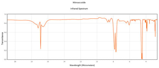
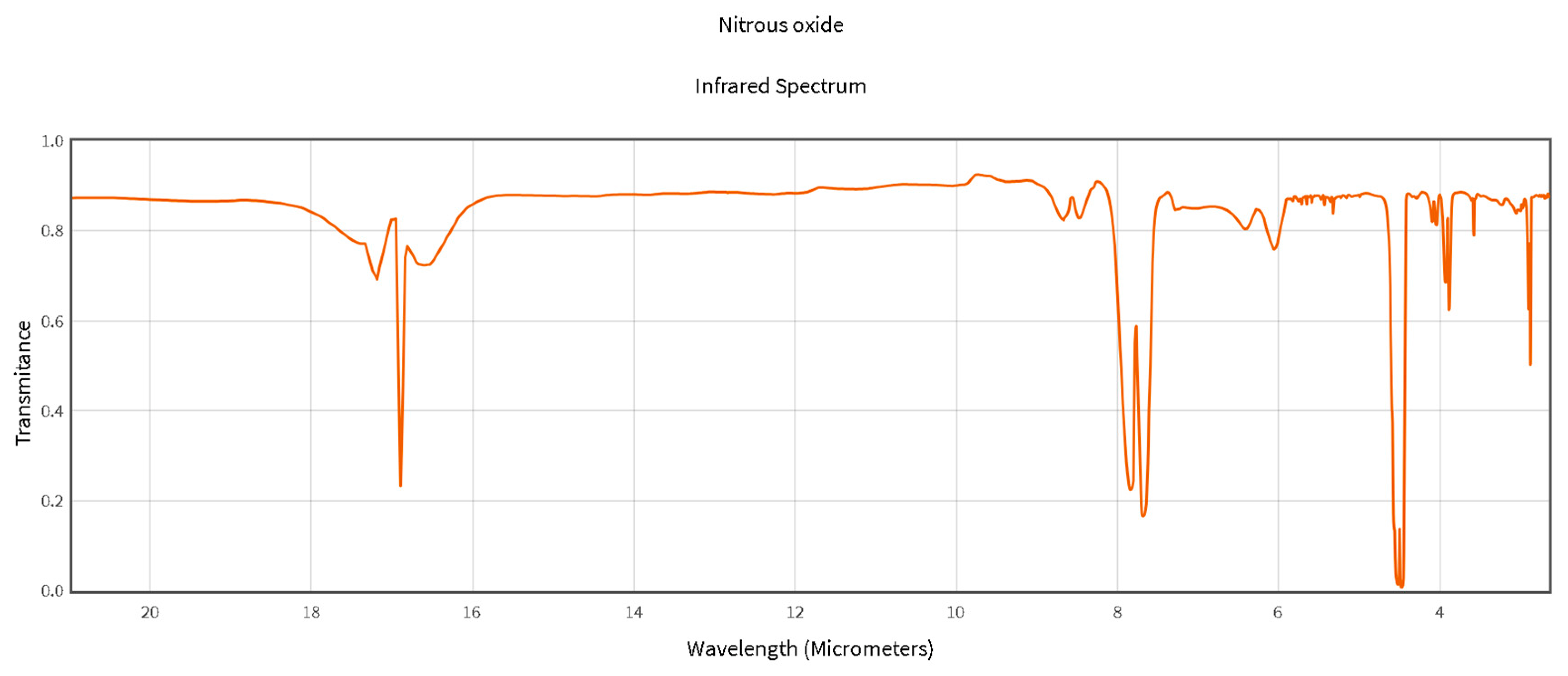
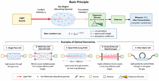
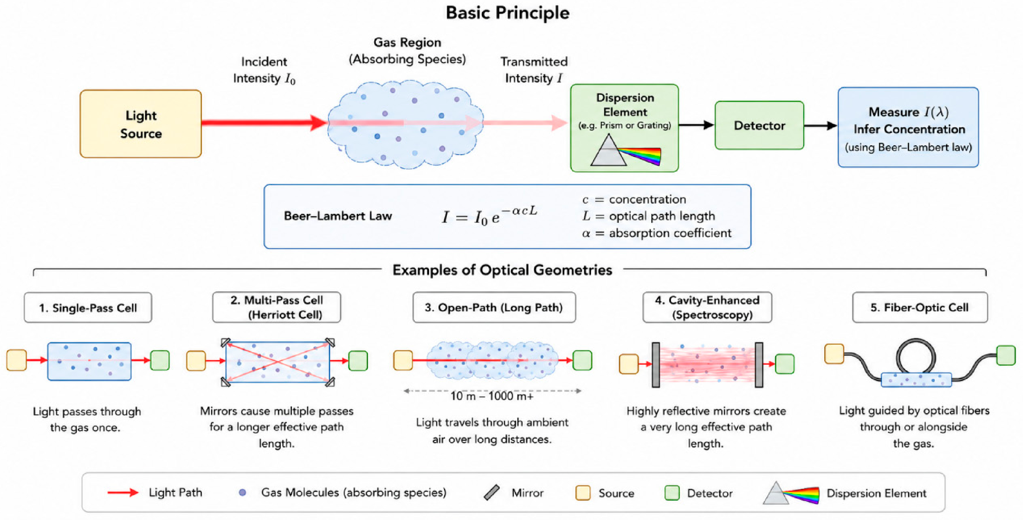

Disclaimer/Publisher’s Note: The statements, opinions and data contained in all publications are solely those of the individual author(s) and contributor(s) and not of MDPI and/or the editor(s). MDPI and/or the editor(s) disclaim responsibility for any injury to people or property resulting from any ideas, methods, instructions or products referred to in the content. |
© 2026 by the authors. Licensee MDPI, Basel, Switzerland. This article is an open access article distributed under the terms and conditions of the Creative Commons Attribution (CC BY) license.