Study on the Contributions of Haze, Fog, Rain, and Snow to Atmospheric Extinction and Low-Visibility Prediction over Eastern China

Abstract

Low visibility (VIS) involves haze, fog, rain, snow, or their combination, while VIS prediction commonly treats aerosol and hydrometeor extinction separately. Observations and the coupled chemistry–weather model are used to quantify their contributions to low VIS in four subregions over eastern China in November 2024. Haze, fog, rain, and snow can all cause low VIS (≤10 km). For 3 < VIS ≤ 10 km and 1 < VIS ≤ 3 km, haze is the most frequent weather record in Harbin and Beijing, whereas fog prevails in Shanghai and Wuhan; for VIS ≤ 1 km, fog dominates in four cities. For 3 < VIS ≤ 10 km, aerosols contribute 87.1–97.3% of the model-estimated total extinction and hydrometeors 2.7–12.8%; for 1 < VIS ≤ 3 km, aerosols contribute 33.9–68.1% and hydrometeors 31.9–66.1%; for VIS ≤ 1 km, hydrometeors contribute 71.6–87.4%, mainly from fog, and fog and snow dominate Northeast China, while aerosols contribute 12.3–28.4%. Jointly considering aerosol and hydrometeor extinction generally produces the lowest root-mean-square error across all VIS grades and the highest threat scores for all VIS levels, especially for VIS ≤ 3 km. These results demonstrate that including both aerosol and hydrometeor extinction is essential for reliable low-VIS prediction.

1. Introduction

Atmospheric visibility (VIS) degradation frequently accompanies haze, fog, rain, and snow and has direct impacts on transportation, aviation, navigation, and public health [1,2]. Light extinction caused by the scattering and absorption of aerosols, fog droplets, and precipitation particles can lead to severe low VIS events [3,4,5]. Fog droplets and precipitation particles are hydrometeors formed through natural microphysical processes in the atmosphere, while aerosols can be emitted mainly from industrial and vehicular sources and from biomass and crop-residue burning [6,7,8,9]. Aerosol extinction generally dominates during haze [10,11,12], while hydrometeor extinction prevails during fog and precipitation [13,14,15], and the two often act jointly during transitions among these weather conditions [16,17,18]. Accurately predicting low VIS therefore requires reasonably quantifying the extinction contributions of aerosols, hydrometeors, and their combination under multiple weather processes.

Numerical prediction based on coupled chemistry–weather models with reliable atmospheric extinction schemes has been widely applied to VIS prediction in many regions [19,20,21]. For both research and operational purposes, different extinction calculation methods are often employed to address low-VIS conditions induced by diverse weather processes. For low VIS induced by aerosol pollution, current extinction algorithms commonly consider aerosol mass concentration, hygroscopic growth, and chemical composition, with some additionally including size distribution and mixing state to better represent aerosol optical properties [22,23,24]. Among commonly used aerosol extinction schemes, empirical relationships directly link VIS or extinction to PM_2.5 and meteorological variables such as relative humidity (RH); these methods are simple but can be strongly data- and region-dependent [25,26]. The Mie theory [27] retrieves aerosol optical properties from particle size distribution and refractive index, which is determined by chemical composition and mixing state; Mie-based calculations are physically detailed but require microphysical and optical information that is not available in every operational system [28]. Chemically speciated mass-reconstruction methods, such as the IMPROVE algorithm, estimate extinction from main aerosol species and corresponding hygroscopic growth factors [29,30]. The IMPROVE algorithm provides more stable performance than empirical fitting methods and Mie model calculations while being simpler to implement [31], and has thus been widely adopted in aerosol extinction calculations [32,33].

When low VIS is accompanied by fog and precipitation, the hydrometeor extinction contribution increases substantially, and most studies apply algorithms that calculate hydrometeor extinction directly, without including aerosol extinction [33,34]. When aerosol particles activate to form fog or cloud droplets under high ambient humidity, or when rain and snow particles are present near the surface, extinction depends on condensed water content, particle or droplet size, number concentration, and hydrometeor phase [1,35]. Fog, rain, and snow are usually parameterized using distinct diagnostic relationships. Low VIS induced by fog has long been linked to liquid water content (LWC) [36], while observations have increasingly shown that droplet number concentration (N_d) also plays an important role, indicating the need for parameterizations that jointly consider LWC and N_d [37,38,39,40]. Rain and snow extinction is commonly derived from precipitation rate or model-predicted hydrometeor mass using empirical or theoretically guided relations [13,41,42]. These methods are convenient for numerical models because the required cloud-water, rain, and snow variables are provided directly by model microphysics.

The individual extinction calculation methods for aerosol and hydrometeor are well established and have been widely applied in low-visibility prediction for the corresponding weather processes. Atmospheric chemistry models typically account for low VIS during haze through aerosol extinction and its hygroscopic growth, while numerical weather models attribute low VIS during fog, rain, and snow to hydrometeor extinction [42,43]. This separation is acceptable when a single weather process clearly dominates, but during haze–fog transitions and aerosol changes with precipitation, considering aerosol or hydrometeor extinction separately often overestimates VIS and misses the observed low-VIS events because each individual component calculation omits the other extinction source [16,21,44].

The coupled chemistry–weather (CW) model GRAPES_Meso5.1/CUACE CW integrates aerosol transport, chemical transformation, and meteorological processes and provides a suitable framework for multicomponent extinction calculations and low-VIS prediction [43]. Previous work has shown that the revised IMPROVE extinction algorithm used in this model captures the VIS variation associated with haze but tends to overestimate extremely low VIS (≤3 km, even ≤1 km) [45]. In this study, the observed relationships among VIS, PM_2.5, RH, and the occurrence of haze, fog, rain, and snow in November 2024 are first analyzed. Three experiments based on this model with identical configurations and driving fields are then conducted for this period, in which VIS is calculated considering aerosol extinction alone, hydrometeor extinction alone, and their combination, respectively. The three experiments are compared at regional and city scales and during typical low-VIS episodes, with particular attention to three VIS grades (3 < VIS ≤ 10 km, 1 < VIS ≤ 3 km, and VIS ≤ 1 km), and the model-estimated relative contributions of aerosol, fog, rain, and snow extinction are quantified for each grade. The performance of the three experiments is finally evaluated with the root-mean-square error (RMSE) for the VIS grades and threat score (TS) for 10, 3, and 1 km VIS levels.

2. Materials and Methods

This section is organized into four parts. Section 2.1 describes the dynamic core, physical and chemical configurations, and the VIS calculation of GRAPES_Meso5.1/CUACE CW, including the aerosol and hydrometeor extinction schemes adopted in this study. Section 2.2 presents the model domain and the experimental design. Section 2.3 describes the emission inventory, meteorological analysis fields, and station observations used for observational analysis and model driving, including the visibility observation methodology and preprocessing. Section 2.4 describes the evaluation metrics and the definitions of the VIS grades and VIS levels used in this study.

2.1. GRAPES_Meso5.1/CUACE CW Model

GRAPES_Meso5.1/CUACE CW is a fully coupled chemistry–weather model that integrates the GRAPES_Meso5.1 mesoscale weather model with the Chinese Unified Atmospheric Chemistry Environment (CUACE) chemistry module [43]. This model includes detailed descriptions of aerosol physical and chemical processes and has been widely applied to VIS, air pollution and dust prediction, pollutant transport, and aerosol–weather interaction studies [45,46,47,48,49,50,51].

The GRAPES_Meso5.1 model [52,53], developed by the China Meteorological Administration (CMA), comprises a fully compressible non-hydrostatic dynamic core and a physical parameterization package. The dynamic core handles the advection and horizontal diffusion of both meteorological and chemical tracers, and the physical package provides multiple physics options for large-scale condensation, cumulus convection, radiation, surface processes, and boundary layer physics [54]. In particular, the Thompson microphysics scheme predicts cloud water, rain, and snow, providing the microphysical quantities required for hydrometeor extinction calculation in this study [55]. The specific physics and chemistry configurations are summarized in Table 1.

The CUACE chemistry model [56] integrates the CAM aerosol module, the CB05CL gaseous chemistry module, and the ISORROPIA II thermodynamic equilibrium module. The CAM module [57] covers sulfate (SF), nitrate (NI), ammonium (AM), organic carbon (OC), elemental carbon (EC), soil dust (SD), and sea salt (SS), and represents key aerosol processes including aerosol generation, hygroscopic growth, aerosol activation, dry and wet deposition, and below-cloud scavenging [50]. Aerosol species are distributed across 12 size bins spanning a radius range of 0.005 to 20.48 μm, except for AM, which uses a single bin. The CB05CL module [58] contains 62 gases and 177 reactions, including 23 photolytic reactions, and the ISORROPIA II module [59] treats gas–particle partitioning and thermodynamic equilibrium.

Table 1. Physical and chemical configurations used in GRAPES_Meso5.1/CUACE CW.

Physical Process	Option	Reference
Advection transport	PRM	Shen et al. [60]
Cumulus convection	Kain-Fritsch ETA	Kain [61]
Cloud microphysics	Thompson	Thompson et al. [55]
Shortwave radiation	Goddard	Chou et al. [62]
Longwave radiation	RRTMG	Price et al. [63]
Surface layer	SFCLAY	Pleim [64]
Planetary boundary layer	MRF	Hong and Pan [65]
Land-surface model	Noah	Ek et al. [66]
Aerosols	CUACE	Gong and Zhang [56]
Gas-phase chemistry	CB05CL	Sarwar et al. [58]
Gas–particle partitioning	ISORROPIA II	Fountoukis and Nenes [59]

Table 1. Physical and chemical configurations used in GRAPES_Meso5.1/CUACE CW.

Physical Process	Option	Reference
Advection transport	PRM	Shen et al. [60]
Cumulus convection	Kain-Fritsch ETA	Kain [61]
Cloud microphysics	Thompson	Thompson et al. [55]
Shortwave radiation	Goddard	Chou et al. [62]
Longwave radiation	RRTMG	Price et al. [63]
Surface layer	SFCLAY	Pleim [64]
Planetary boundary layer	MRF	Hong and Pan [65]
Land-surface model	Noah	Ek et al. [66]
Aerosols	CUACE	Gong and Zhang [56]
Gas-phase chemistry	CB05CL	Sarwar et al. [58]
Gas–particle partitioning	ISORROPIA II	Fountoukis and Nenes [59]

VIS in this model is calculated from the Koschmieder relationship between VIS and the near-surface extinction coefficient [67], with the total atmospheric extinction (b_ext) expressed in Mm⁻¹ and VIS in km:

VIS = 1000∙K/b_ext

(1)

where K = 3.912, corresponding to a contrast threshold of 0.02 [67].

For aerosol extinction calculations, the revised IMPROVE algorithm is adopted in this study. In this scheme, SF, NI, and organic matter (OM) are each partitioned into small and large modes based on mass concentration, with mode-specific dry mass extinction efficiencies and hygroscopic growth factors assigned accordingly; the scheme adopts an OM-to-OC conversion factor of 1.8 and additionally includes sea salt extinction with hygroscopic growth, nitrogen dioxide (NO₂) absorption, and Rayleigh scattering [30]. The extinction contributions from aerosols (b_{ext_aero}, Mm⁻¹) in this study are then calculated as

$$\begin{array}{c}{b}_{\mathit{ext}\_\mathit{aero}}=2.2f_S\left(\mathit{RH}\right)[\mathit{Small} \mathit{SF}]+4.8f_L\left(\mathit{RH}\right)[\mathit{Large} \mathit{SF}]+2.4f_S\left(\mathit{RH}\right)[\mathit{Small} \mathit{NI}]+5.1f_L\left(\mathit{RH}\right)[\mathit{Large} \mathit{NI}]\hfill \\ \hspace{1em}\hspace{1em}\hspace{1em}\hspace{1em}\hspace{1em}\hspace{1em}+2.8[\mathit{Small} \mathit{OM}]+6.1[\mathit{Large} \mathit{OM}]+10\left[\mathit{EC}\right]+\left[\mathit{Soils}\right]+1.7f_{\mathit{SS}}\left(\mathit{RH}\right)\left[\mathit{SS}\right]+0.6\left[\mathit{CM}\right]\hfill \\ \hspace{1em}\hspace{1em}\hspace{1em}\hspace{1em}\hspace{1em}\hspace{1em}+0.33\left[{\mathit{NO}}_2\right(\mathit{ppb}\left)\right]+b_{\mathit{rayleigh}}\hfill \end{array}$$

(2)

where f_S(RH), f_L(RH), and f_SS(RH) are the hygroscopic growth factors for the small mode, large mode, and sea salt, respectively, with values adopted from the IMPROVE program (available at https://vista.cira.colostate.edu/Improve/ (accessed on 4 May 2026)) (Figure S1). [SF], [NI], [OM], [EC], [Soils], [SS] and [CM] (coarse mass, aerodynamic diameter 2.5–10 μm) denote the mass concentrations (μg m⁻³) of the corresponding aerosol species. Large and Small denote the size modes for SF, NI, and OM [30]. The Rayleigh scattering coefficient b_rayleigh is fixed at 10 Mm⁻¹.

For the extinction contributed by fog, rain, and snow, this study adopts the bulk framework proposed by Stoelinga and Warner [42], as implemented in version 2.2 of the Unified Post Processor (UPP2.2) developed by the U.S. National Centers for Environmental Prediction (NCEP). The total hydrometeor extinction (b_{ext_hydro}, Mm⁻¹) is calculated as

b_{ext_hydro} = 10³∙(b_{ext, fog} + b_{ext, rain} + b_{ext, snow})

(3)

where the subscripts fog, rain, and snow denote near-surface cloud water, rain, and snow at the lowest model level, respectively; each component is expressed in km⁻¹, and the factor 10³ converts the sum to Mm⁻¹.

For rain and snow, the original UPP2.2 bulk relations are applied unchanged:

$$b_{\mathit{ext},\mathit{rain}}=2.24·C_{\mathit{rain}}^{0.75}; b_{\mathit{ext},\mathit{snow}}=10.36·C_{\mathit{snow}}^{0.78}$$

(4)

where C_rain and C_snow are the near-surface mass concentrations (g m⁻³) of rain and snow, respectively.

The original bulk fog relation, which scales with liquid water content alone, is superseded by the formulation of Gultepe et al. [39], in which extinction is governed jointly by the mass concentration (C_fog, g m⁻³) and the number concentration (N_d, cm⁻³) of fog droplets:

$$b_{\mathit{ext},\mathit{fog}}=4.46{·(C_{\mathit{fog}}·N_d)}^{0.49}$$

(5)

Both C_fog and N_d are taken from the lowest model level. The N_d is a diagnosed quantity obtained through the grid-scale aerosol–cloud coupling of the model [43,51]: the CUACE aerosol module provides the real-time number concentration of hydrophilic aerosols in 12 size bins spanning 0.005–20.48 μm, from which the activated fraction at the ambient supersaturation is computed following the Köhler theory look-up-table approach of Thompson and Eidhammer [68], with the activation fraction determined by temperature, vertical velocity, aerosol number concentration, and the prescribed hygroscopicity parameter and mean radius [69]; the activated droplet number concentration is passed to the Thompson microphysics scheme and is adopted as the N_d in Equation (5).

The total atmospheric extinction combines the aerosol and hydrometeor components:

b_{ext_total} = b_{ext_aero} + b_{ext_hydro}

(6)

The resulting total extinction is converted to VIS through the Koschmieder relationship (Equation (1)). This linear superposition rests on the independent-scattering approximation, whereby distinct particles attenuate light additively while multiple scattering and mutual shadowing are neglected [70]. Several constraints are applied to ensure physically reasonable extinction estimates. The hygroscopic growth factors of the revised IMPROVE algorithm are defined only up to 95% RH [30], so the model RH used to determine them is capped at 95%, with the growth factors at 95% RH applied whenever the modeled RH exceeds this value (Figure S1). To avoid double counting between aerosol hygroscopic growth and fog-droplet extinction, the fog term is activated only when the near-surface RH ≥ 95% and the lowest-level cloud-water mixing ratio exceeds 0.015 g kg⁻¹, following UPP2.2 [71], and the rain and snow terms are active whenever their respective hydrometeor mass concentrations are nonzero.

2.2. Model Domain and Experimental Design

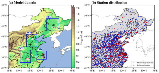
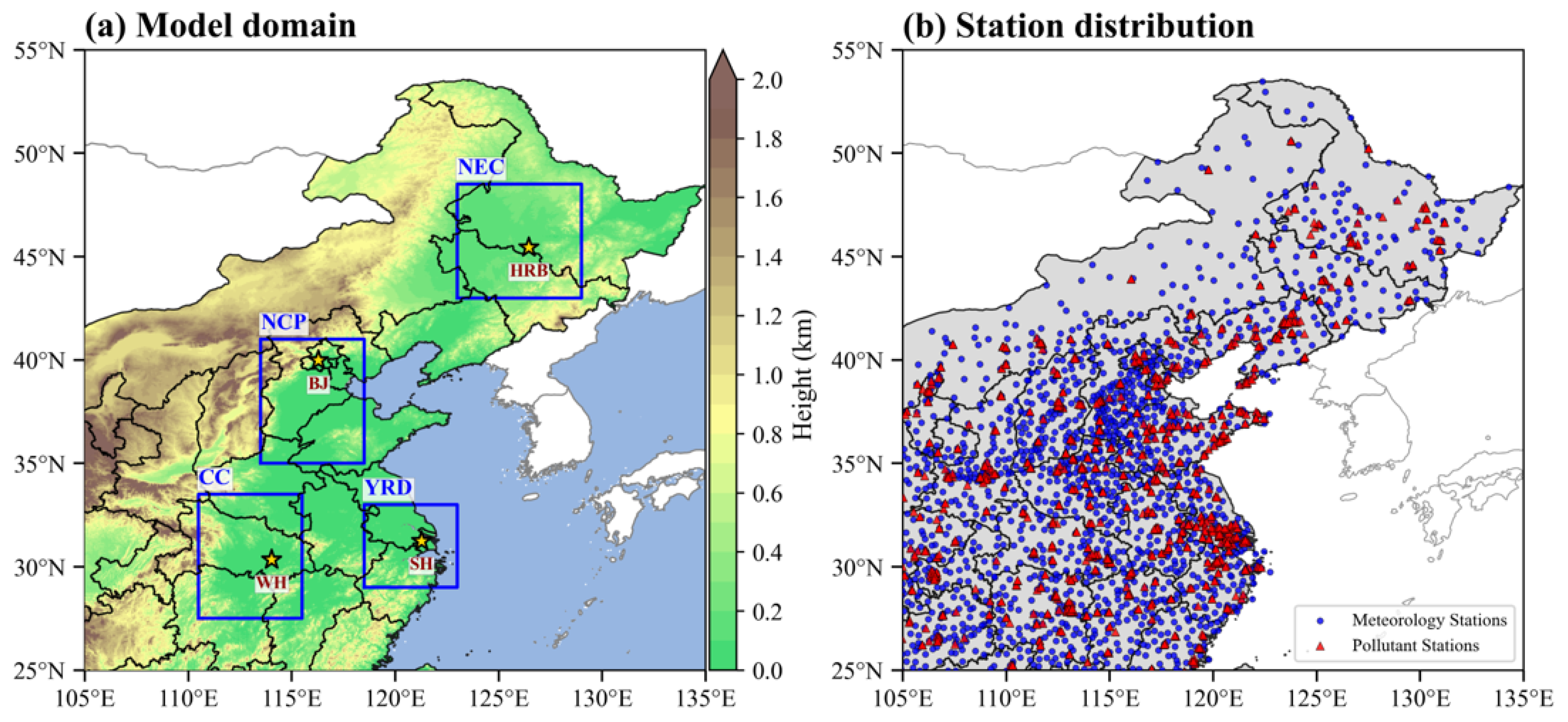
In this study, the model domain covers eastern China (25.0–55.0° N, 105.0–135.0° E, Figure 1a) with 0.1° × 0.1° horizontal resolution and 49 vertical layers extending from the surface to approximately 31 km. The lowest model level is located at approximately 52 m above the surface in the terrain-following coordinate, varying little across the study domain. The model was run from 28 October to 30 November 2024, cycled every 72 h, with hourly output. The simulations of the first cycle were discarded as spin-up, and the simulation results during 1–30 November were used for evaluation. A multiyear climatological chemical field was used for the first initialization, and subsequent cycles were warm-started from the chemical tracer fields of the preceding cycle [43].

Figure 1. (a) Model domain and topography, with the key subregions indicated by blue boxes and the representative cities by yellow stars. Panel (b) shows the locations of meteorological stations (purple dots) and PM_2.5 observation stations (red triangles).

The three experiments (EXPs, Table 2) use identical model configurations, meteorological driving fields, and chemical input data; they differ only in the extinction components included in the VIS calculation. EXP1 retains aerosol extinction together with NO₂ absorption and Rayleigh scattering, following the revised IMPROVE algorithm [30]; EXP2 calculates extinction from near-surface fog/cloud water, rain, and snow, with rain and snow following the UPP2.2 bulk formulations [42] and fog following Gultepe et al. [39]; and EXP3 sums the extinction components represented in EXP1 and EXP2 before converting total extinction to VIS.

Table 2. Experimental design in this study.

Experiment	Description
EXP1	Aerosol extinction (bext_aero): chemically speciated aerosol extinction with hygroscopic growth, plus NO2 absorption and Rayleigh scattering, following the revised IMPROVE algorithm [30].
EXP2	Hydrometeor extinction (bext_hydro): rain and snow extinction following the UPP2.2 bulk formulations [42], with fog extinction following Gultepe et al. [39].
EXP3	Total extinction (bext_total): sum of all components in EXP1 and EXP2 (bext_aero + bext_hydro) before conversion to VIS.

To sample contrasting combinations of aerosol loading and hydrometeor occurrence across eastern China during the study period, four subregions were delineated: Northeast China (NEC, 43.0–48.5° N, 123.0–129.0° E), where multiphase precipitation coincided with high aerosol loading during November 2024; the North China Plain (NCP, 35.0–41.0° N, 113.5–118.5° E), which experienced low VIS involving severe haze and rapid transitions among haze, fog, and precipitation during the study period; the Yangtze River Delta (YRD, 29.0–33.0° N, 118.5–123.0° E), with lower emissions, where fog and liquid-phase precipitation prevailed during November 2024; and Central China (CC, 27.5–33.5° N, 110.5–115.5° E), similar to the NCP but with more frequent fog and precipitation throughout the study period. The city-scale evaluation focuses on four representative cities: Harbin (HRB, 45.5° N, 126.5° E), Beijing (BJ, 40.0° N, 116.3° E), Shanghai (SH, 31.2° N, 121.3° E), and Wuhan (WH, 30.4° N, 114.0° E). The locations of the key subregions and representative cities are shown in Figure 1a.

2.3. Data Used

The datasets used in this study comprise meteorological and chemical inputs for the coupled model and station observations for observational analysis and model evaluation. The anthropogenic emissions were obtained from the Multi-Resolution Emission Inventory for China (MEIC) provided by Tsinghua University (http://meicmodel.org.cn/ (accessed on 4 May 2026)), as described by Zheng et al. [72]. The gaseous and particulate emissions were mapped to the chemical species and grid required by CUACE before use [73]. The NCEP Final Operational Global Analysis (FNL, https://rda.ucar.edu/datasets/ds083.3/ (accessed on 4 May 2026)) at 0.25° × 0.25° horizontal resolution and 6 h intervals provided the meteorological initial and lateral boundary conditions.

Hourly observed VIS (km), RH (%), precipitation (mm), and weather records were obtained from approximately 2400 CMA stations (http://data.cma.cn (accessed on 4 May 2026)). The instrument types, installation, calibration, observation procedures, and data processing follow the unified specifications of the CMA surface observation system [74,75]; all data passed strict quality control before use, and only records marked as ‘good’ were retained. Hourly PM_2.5 concentrations (μg m⁻³) were obtained from approximately 1500 stations operated by the China National Environmental Monitoring Centre (http://www.cnemc.cn (accessed on 4 May 2026)). These data were subjected to additional quality control following Zhong et al. [76]: values deviating from the 1-month moving average at each site by more than three standard deviations were excluded. The locations of the observation stations are shown in Figure 1b. All observational and simulated data were converted to UTC before analysis.

VIS is continuously monitored by meteorological optical rangefinders operating on transmission or scattering principles, which report the meteorological optical range (MOR), i.e., the path length over which the luminous flux of a collimated beam is attenuated to 5% of its initial value (contrast threshold 0.05, K = 2.996) [77]. Meteorological VIS is defined at a contrast threshold of 0.02 (K = 3.912) [67], and the instrument-measured MOR has been converted to VIS according to the theoretical ratio of 2.996/3.912 derived from the Lambert–Bouguer and Koschmieder laws [78,79]; the released VIS product is therefore consistent with the Koschmieder definition of Equation (1). The coefficient 3.912 is also widely used in VIS studies based on the IMPROVE algorithm [31,80,81,82] and is the standard formulation in the VIS algorithms of the bulk-extinction framework [42]. To ensure data reliability, VIS was restricted to the range of 0–30 km: observed values of 30 km and above were capped at 30 km, samples with VIS = 0 km were removed, and the same limits were applied to the simulated VIS. The low-visibility grades (≤10 km) are the focus of this study; therefore, the truncation has little effect on the grade-based evaluation or on the relative performance of the three experiments.

Following World Meteorological Organization (WMO) Code Table 4677 [83], each station-hour provides one designated present-weather record, allowing each sample to be assigned to one of five categories: haze, fog, rain, snow, or other (Table S1). All records are produced automatically: precipitation phenomena are identified by precipitation phenomenon sensors, and visibility-obstruction phenomena (fog, mist, haze, and dust) are generated by the national-level multi-source integrated discrimination from surface VIS, RH, and related meteorological variables; when multiple phenomena coexist within one hour, the highest applicable code figure is selected [83]. In Table S1, mist (ww = 10; VIS of 1–10 km reduced by suspended droplets) and shallow fog (ww = 11–12) are grouped with ‘fog’, and drizzle (ww = 20, 50–57) is grouped with ‘rain’, according to their extinction mechanisms. Note that the present-weather record does not exclude co-occurring hydrometeors or aerosol pollution.

2.4. Evaluation Metrics

For model evaluation, the simulated VIS at the nearest model grid point to each station was paired with the station observation, and only pairs with valid observations were retained. Three metrics are used to evaluate the paired samples: the root-mean-square error (RMSE), the Pearson correlation coefficient (R), and the threat score (TS).

The RMSE is defined as

$$\mathit{RMSE}={\left[\left({\displaystyle \frac{1}{N}}\right){\displaystyle {\sum }_{i=1}^N}{({\mathit{VIS}}_{\mathit{sim},i}-{\mathit{VIS}}_{\mathit{obs},i})}^2\right]}^{1/2}$$

(7)

where N is the number of valid pairs, VIS_sim denotes the simulated VIS, and VIS_obs denotes the observed VIS.

The R is defined as

$$R={\displaystyle \frac{{\sum }_{i=1}^N({\mathit{VIS}}_{\mathit{sim},i}-{\overline{\mathit{VIS}}}_{\mathit{sim}})({\mathit{VIS}}_{\mathit{obs},i}-{\overline{\mathit{VIS}}}_{\mathit{obs}})}{\sqrt{{\sum }_{i=1}^N{({\mathit{VIS}}_{\mathit{sim},i}-{\overline{\mathit{VIS}}}_{\mathit{sim}})}^2·{\sum }_{i=1}^N{({\mathit{VIS}}_{\mathit{obs},i}-{\overline{\mathit{VIS}}}_{\mathit{obs}})}^2}}}$$

(8)

where the overbars denote the mean values, and is used to measure the temporal covariation between simulated and observed VIS.

For a given VIS threshold V, the TS is defined as

$$\mathit{TS}={\displaystyle \frac{H}{H+M+F}}$$

(9)

where H, M, and F denote the numbers of hits (both observed and simulated VIS ≤ V), misses (observed VIS ≤ V but simulated VIS > V), and false alarms (simulated VIS ≤ V but observed VIS > V), respectively.

The component fractions are computed as the arithmetic mean of the individual sample fractions, and all station-hour samples are equally weighted with no area weighting. The RMSE and the extinction-fraction analysis are reported for three mutually exclusive VIS grades (3 < VIS ≤ 10 km, 1 < VIS ≤ 3 km, and VIS ≤ 1 km), which are defined solely by the observed station-hour VIS; the same valid station-hour samples are used to evaluate all three experiments, so their RMSE values are directly comparable. Separately, the TS is evaluated at three cumulative VIS levels (VIS ≤ 10, 3, and 1 km). For a given threshold, the TS incorporates all events with visibility at or below that threshold, which emphasizes the model performance for low-visibility conditions.

3. Results and Discussion

Severe and widespread VIS degradation in eastern China is often associated with haze, fog, rain, or snow [26,33]. November 2024 contains several regional low-VIS episodes involving different weather processes and is therefore selected for the controlled comparison of the three experiments. Section 3.1 examines the observed relationships among VIS, PM_2.5, and RH, and the accompanying weather records for the three VIS grades. Section 3.2 evaluates the performance of the three experiments at regional and city scales and during typical low-VIS episodes. Section 3.3 statistically evaluates the modeled low VIS (≤10 km) in the three experiments, with particular attention to severely low VIS (≤3 km) and extremely low VIS (≤1 km).

3.1. Characteristics of Observed Low VIS Under Haze, Fog, Rain, and Snow

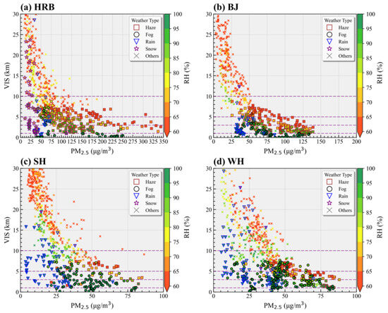
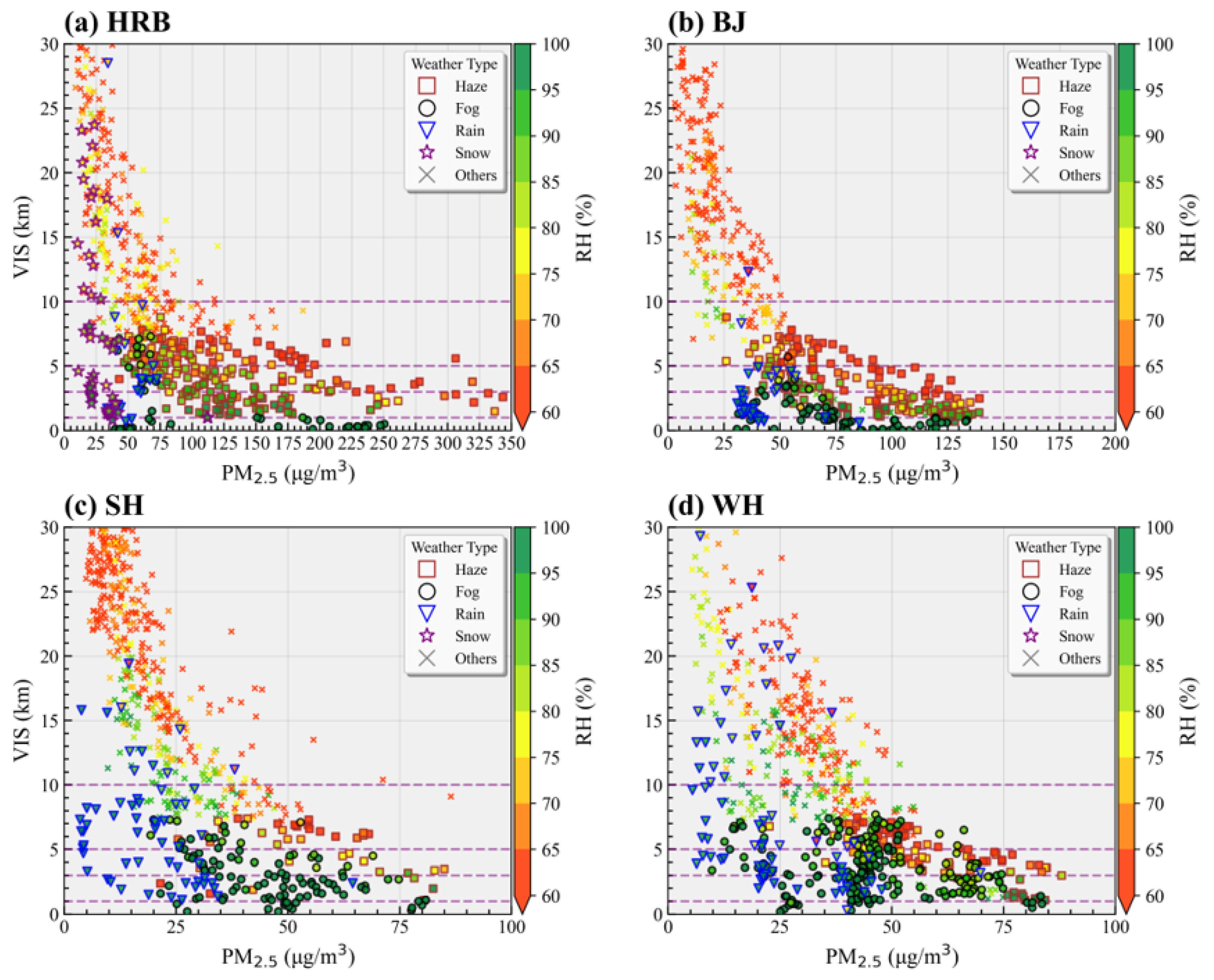
PM_2.5 concentration and ambient RH are the most important factors influencing VIS [84,85], and their relationship with VIS varies considerably across regions and weather conditions. Figure 2 shows the relationship between hourly observed VIS and PM_2.5 under different RH conditions in the four representative cities in November 2024, with marker shape distinguishing weather records. Haze, fog, rain, and snow can all lead to low VIS (≤10 km). Under relatively dry conditions (RH < 80%), VIS generally exhibits an inverse relationship with PM_2.5, and weather records predominantly show haze, indicating that aerosol extinction dominates the VIS degradation [86]. Under high-RH conditions (80% ≤ RH < 95%), a given PM_2.5 concentration corresponds to lower VIS, which reflects enhanced extinction from aerosol hygroscopic growth [80,87], and rain or snow under high RH can also reduce VIS substantially. Near saturation (RH ≥ 95%), fog occurs frequently and results in extremely low VIS (≤1 km) [88].

Figure 2. Relationship between hourly observed visibility (VIS) and PM_2.5 concentration in (a) Harbin (HRB), (b) Beijing (BJ), (c) Shanghai (SH), and (d) Wuhan (WH) in November 2024. Marker color denotes relative humidity (RH), and marker shape denotes the weather records (haze, fog, rain, snow, or other).

The weather processes associated with low VIS also differ across the different VIS grades and among the four representative cities (the percentages reported below are calculated relative to all valid hourly samples with VIS ≤ 10 km in each city during November 2024; Table S2). For 3 < VIS ≤ 10 km, haze dominates the records in HRB (37.5%) and BJ (27.9%), and fog is the most frequent record in SH (17.8%) and WH (26.8%), exceeding haze (13.6% and 17.8%, respectively). Rain occurs most frequently in SH (9.9%) and is minor elsewhere (1.0–3.6%). For 1 < VIS ≤ 3 km, haze remains the most frequent record in HRB (17.1%) and BJ (24.1%), and fog prevails in SH (18.6%) and WH (19.0%). Rain occurs in all four cities (1.3–3.7%), and snow appears in HRB (3.5%). For VIS ≤ 1 km, haze is nearly absent in all four cities (0–1.2%), fog accounts for most of the records, and rain (0.5–1.8%) and snow (0.8%) contribute only minor shares, with snow occurring in HRB only. Overall, haze records account for 54.7% and 53.1% of the low-VIS samples in HRB and BJ and 16.1% and 20.9% in SH and WH; fog records account for 42.2% and 49.9% in SH and WH and 11.1% and 19.9% in HRB and BJ, indicating that low VIS in the northern cities is more frequently associated with haze and snow, whereas that in the southern cities is more frequently associated with fog and rain. These weather records are used only to describe the synoptic context of the low-VIS samples, such as which weather processes dominate in each city and grade; they are not treated as independent evidence for attributing extinction in this study.

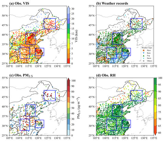
Multiple weather processes can also act within a single synoptic period (Figure 3). From 21:00 UTC 13 November to 03:00 UTC 14 November 2024, observed VIS was generally lower than 10 km, reaching 0–1 km in much of the NCP and YRD and 1–3 km in the CC and NEC (Figure 3a). In the NCP, YRD, and CC, the low VIS coincides with widespread fog and rain records with high RH (>85%) (Figure 3b,d). Observed PM_2.5 was about 40–60 μg m⁻³ in the YRD and CC and over 75 μg m⁻³ in the NCP (Figure 3c). The NEC exhibits severe low VIS with high PM_2.5, and its weather records involve snow, fog, and haze (Figure 3b,c). Different weather processes act together to reduce VIS over different regions within a single period, indicating that a VIS scheme considering aerosol or hydrometeor extinction separately is insufficient for such compound conditions. Moreover, the rain records in such episodes may partly arise from drizzle, which is coded as ‘rain’ under the present-weather classification but may contribute extinction through the modeled fog term because of its small droplets. The model-estimated fog and rain extinction accordingly carries additional uncertainty, particularly in the YRD and CC, where drizzle frequently accompanies fog [89].

Figure 3. Mean (a) observed (Obs.) visibility (VIS), (b) weather records, (c) Obs. PM_2.5, and (d) Obs. RH from 21:00 UTC 13 November to 03:00 UTC 14 November 2024.

Given that aerosol and direct hydrometeor extinction can coexist, with their relative contributions varying with humidity, weather process, and different VIS grades, the following section uses the three experiments to compare the three extinction representations and examine how their differences evolve across representative low-visibility episodes and the three VIS grades.

3.2. Performance of the Three Experiments in Low-VIS Prediction

Severe VIS reduction can result from aerosol extinction during haze and from hydrometeor extinction during fog, rain, and snow. The three experiments share identical meteorological and chemical fields (Figures S2 and S3) and differ only in the extinction components included in the VIS calculation; their differences therefore isolate the contributions of aerosol and hydrometeor extinction during typical low-VIS episodes.

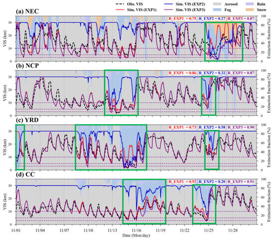
Figure 4 compares the observed and simulated hourly VIS over the four key subregions, with background shading showing the fractional contributions of aerosol, fog, rain, and snow to the total modeled extinction in EXP3. EXP1 reproduces the observed VIS variations reasonably in all four regions, with R of 0.75, 0.86, 0.73, and 0.92 in the NEC, NCP, YRD, and CC, respectively, although it overestimates VIS during some hydrometeor-affected episodes (green boxes). EXP3 increases the correlation in the NEC (0.87) and YRD (0.90), remains nearly unchanged in the NCP (0.87), and is slightly lower in the CC (0.91). EXP2 is only weakly correlated with observed VIS except in the YRD, where its R reaches 0.58; elsewhere, it often remains near the 30 km upper bound except during fog and precipitation episodes. The background fractions show that aerosol extinction provides the persistent contribution throughout the month, and fog, rain, or snow becomes dominant only during hydrometeor-affected episodes, which explains why the differences between EXP3 and EXP1 are most evident in the NEC and YRD.

Figure 4. Hourly visibility (VIS) in (a) Northeast China (NEC), (b) North China Plain (NCP), (c) Yangtze River Delta (YRD), and (d) Central China (CC). Black dashed lines denote observations; red, blue, and purple lines denote EXP1, EXP2, and EXP3, respectively. Background shading shows the fractional contributions of aerosol, fog, rain, and snow to total modeled extinction in EXP3. The green boxes denote episodes affected by hydrometeors within the study period (1–30 November 2024).

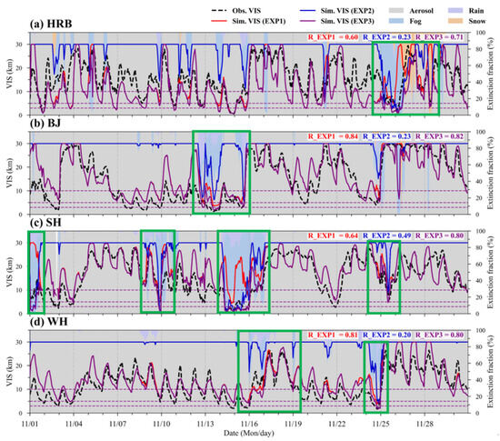
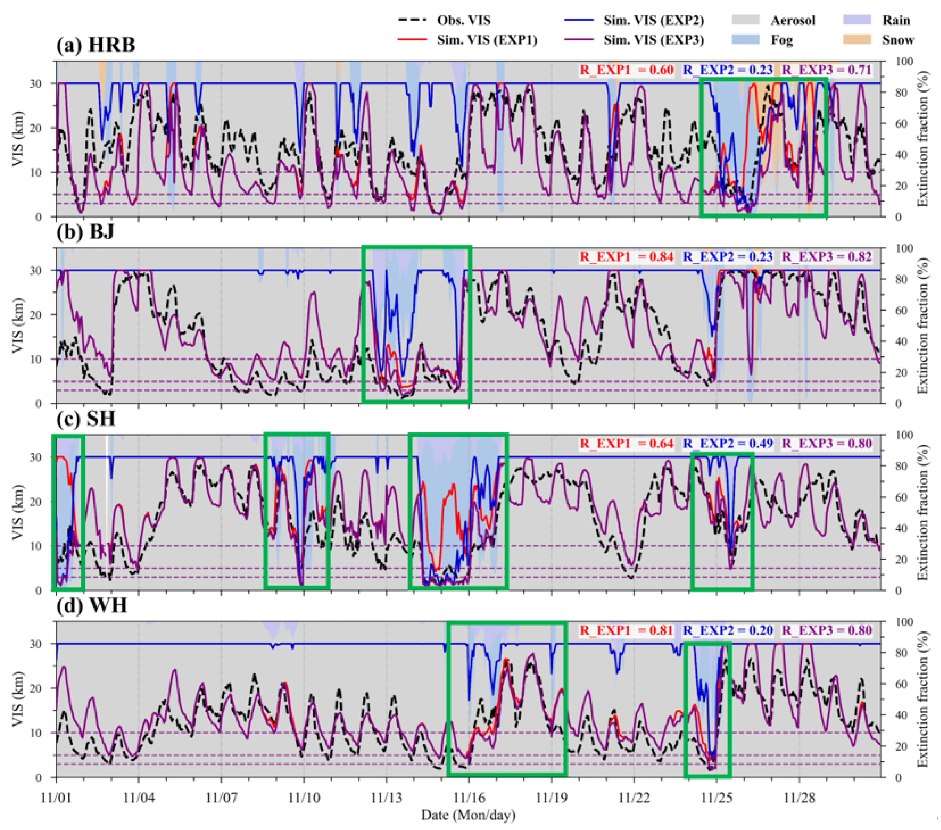
At the city scale (Figure 5), the performance differences among the three experiments also differ among the four cities. EXP1 attains R of 0.60, 0.84, 0.64, and 0.81 in HRB, BJ, SH, and WH, respectively. EXP3 increases the correlation to 0.71 in HRB and 0.80 in SH but slightly decreases it to 0.82 in BJ and 0.80 in WH. Thus, the combined extinction calculation does not uniformly increase the temporal correlation. EXP2 shows moderate correlation in SH (0.49) but remains weak in HRB, BJ, and WH (0.20–0.23). These city-level differences are consistent with the regional patterns and indicate that the simulated hydrometeor occurrence controls when EXP2 or EXP3 departs from EXP1.

Figure 5. Hourly visibility (VIS) in (a) Harbin (HRB), (b) Beijing (BJ), (c) Shanghai (SH), and (d) Wuhan (WH). Black dashed lines denote observations; red, blue, and purple lines denote EXP1, EXP2, and EXP3, respectively. Background shading shows the fractional contributions of aerosol, fog, rain, and snow to total modeled extinction in EXP3. The green boxes denote episodes affected by hydrometeors within the study period (1–30 November 2024).

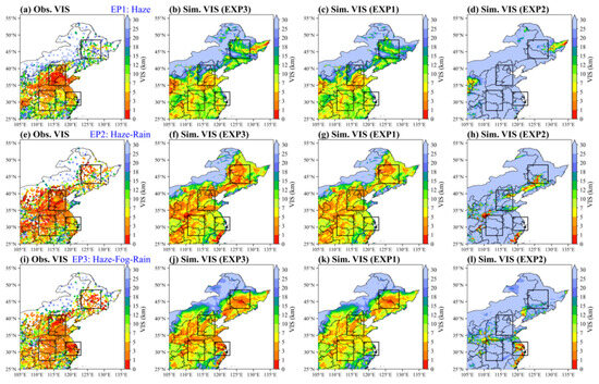
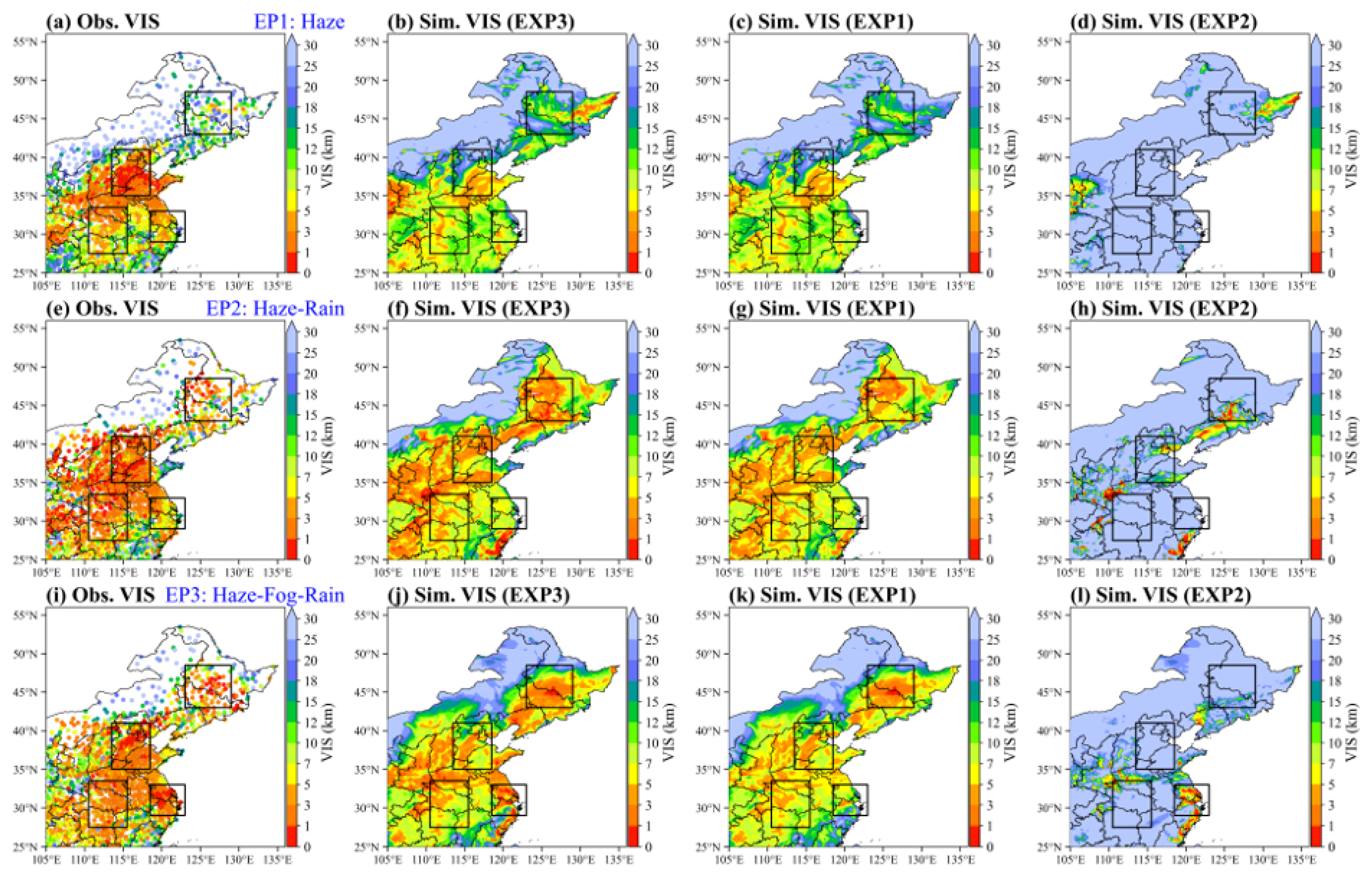
Figure 6 isolates three episodes (EPs) selected according to the temporal evolution of observed VIS, PM_2.5, precipitation, and RH over the NCP and YRD (Figure 4 and Figure S3). During EP1 (haze; 21:00 UTC 11 November to 03:00 UTC 12 November), EXP1 and EXP3 are spatially similar over most key subregions and EXP2 is confined to limited areas, consistent with the dominant aerosol contribution supported by the PM_2.5 enhancement and generally weak precipitation (Figure S4). During EP2 (haze–rain; 21:00 UTC 13 November to 03:00 UTC 14 November), modeled rain structures produce narrow low-visibility features in EXP2, while EXP1 retains the broader aerosol-related pattern and EXP3 contains both contributions (Figure S5). During EP3 (haze–fog–rain; 21:00 UTC 14 November to 03:00 UTC 15 November), fog becomes widespread after the preceding precipitation and aerosol changes, especially over the YRD and its adjacent coastal areas; the low-VIS areas in EXP2 expand accordingly, and EXP3 departs more strongly from EXP1 in the fog-affected areas (Figure S6). Across the three episodes, EXP3 more closely matches the observed low-VIS areas than EXP1 and EXP2, although it broadens or deepens some low-VIS areas relative to observations.

Figure 6. Mean visibility (VIS) for three low-VIS episodes (EPs); columns show, from left to right, observed (Obs.) VIS and simulated (Sim.) VIS from EXP3, EXP1, and EXP2: (a–d) EP1 (21:00 UTC 11 November to 03:00 UTC 12 November), (e–h) EP2 (21:00 UTC 13 November to 03:00 UTC 14 November), and (i–l) EP3 (21:00 UTC 14 November to 03:00 UTC 15 November 2024).

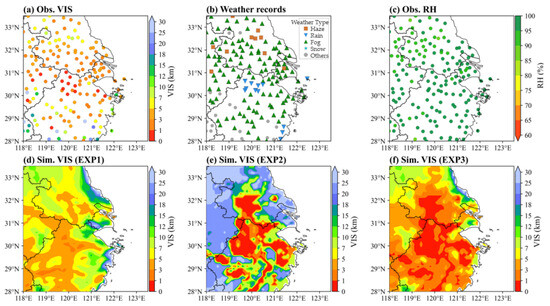
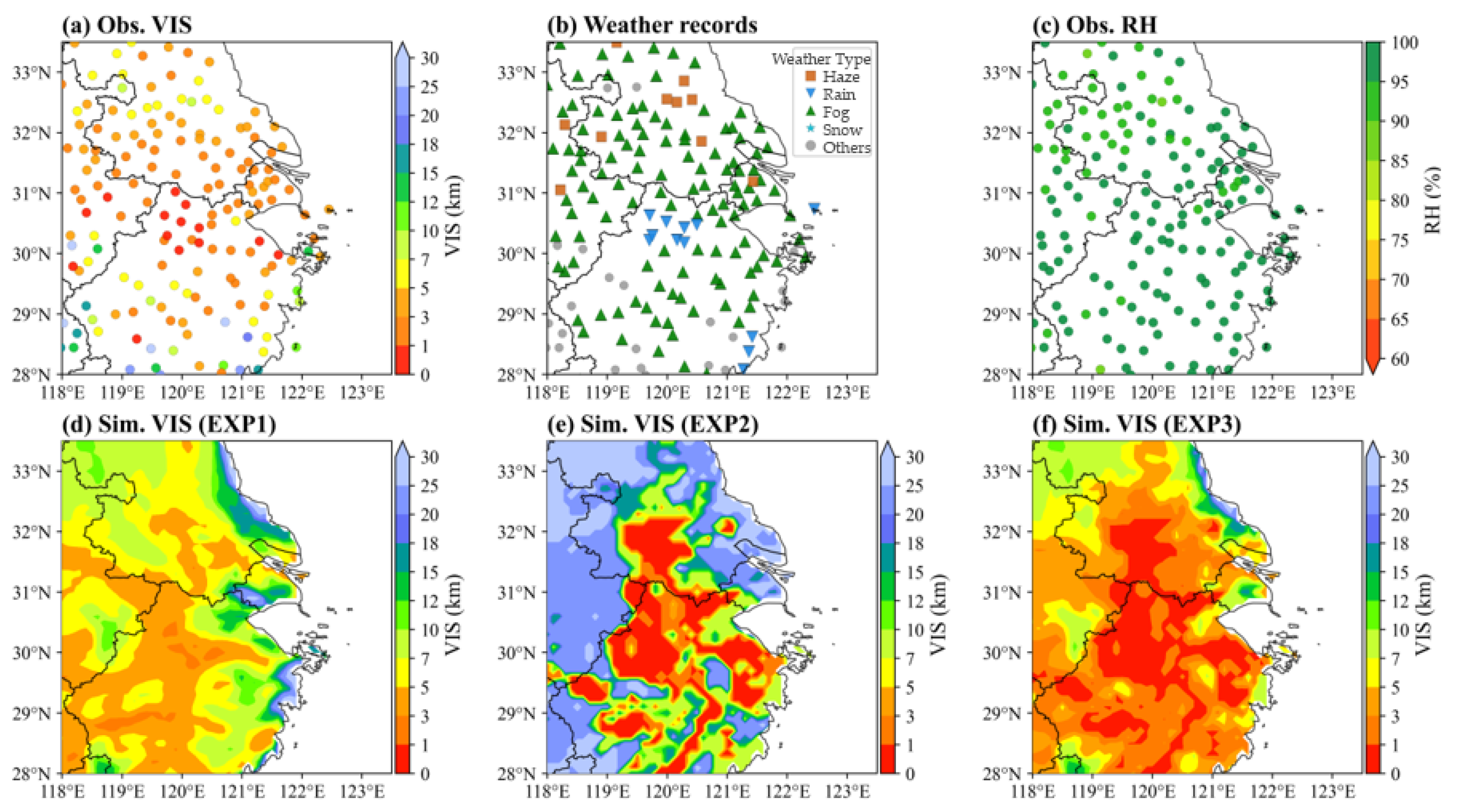
Figure 7 presents a focused YRD case dominated by fog. From 21:00 UTC 15 November to 00:00 UTC 16 November, fog is reported at most YRD stations, RH commonly exceeds 90%, PM_2.5 is generally modest, and precipitation is weak (Figure S7). EXP1 captures the minor aerosol contribution but overestimates VIS, and EXP2 reproduces the widespread low VIS associated with fog. EXP3 combines both contributions and better reproduces the observed VIS ≤ 3 km, demonstrating that this low VIS arises from hydrometeor extinction superimposed on the aerosol background, in line with recent findings for haze–fog processes in SH and eastern China [44].

Figure 7. Mean (a) observed (Obs.) visibility (VIS), (b) weather records, (c) Obs. relative humidity (RH), (d–f) simulated (Sim., EXP1, EXP2, and EXP3) VIS from 21:00 UTC 15 November to 00:00 UTC 16 November 2024.

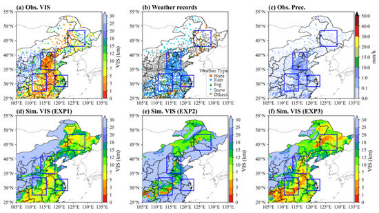
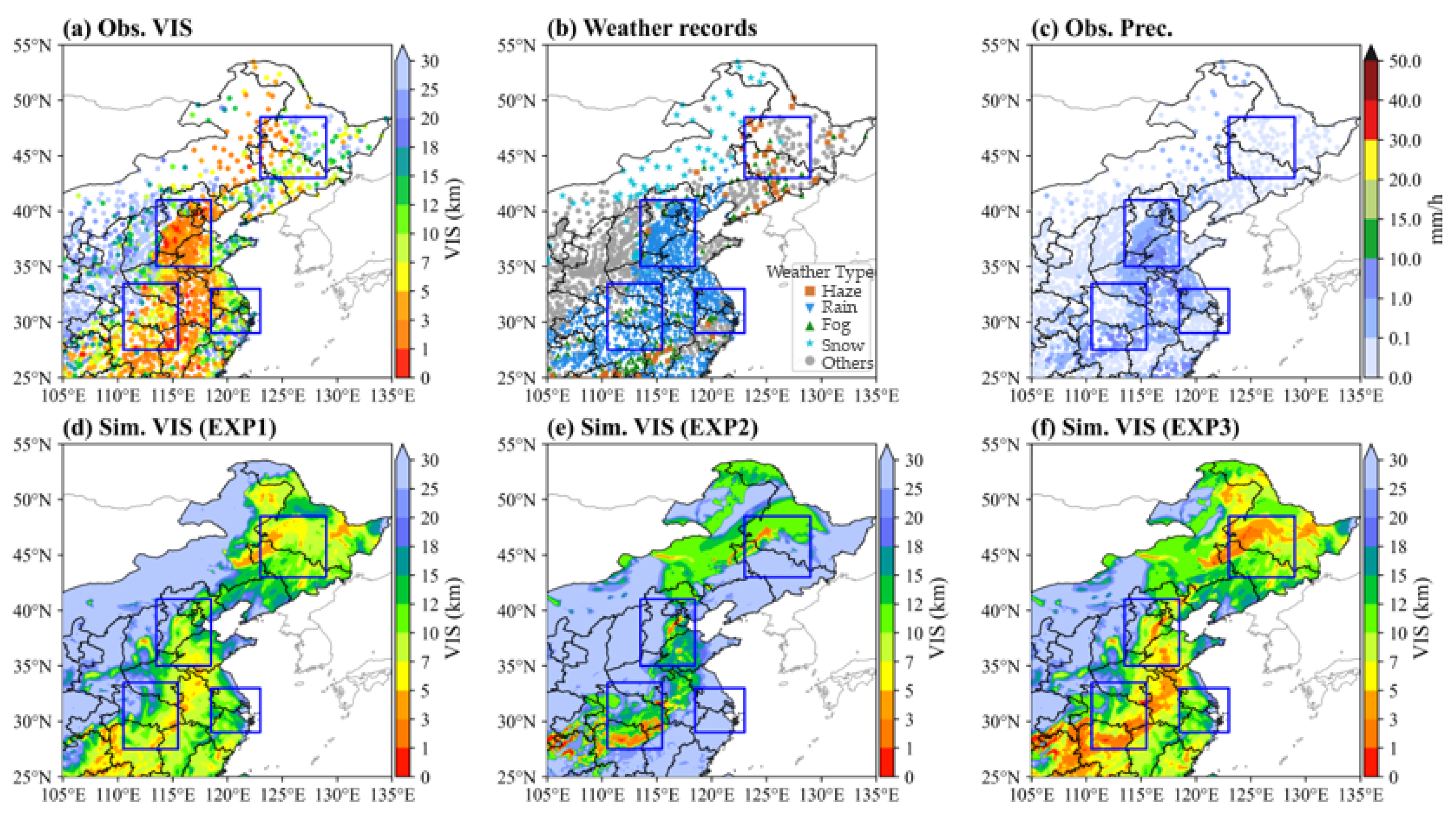
The 24–25 November event provides a typical case involving rain and snow extinction (Figure 8). From 22:00 UTC 24 November to 00:00 UTC 25 November, observed low VIS extended along a broad rain corridor across the NCP, YRD, and CC (Figure S8), while snow was recorded further north in the NEC. EXP1 and EXP2 depict the aerosol and hydrometeor contributions separately along the modeled precipitation corridor, and EXP3 includes both. The model reproduces the broad precipitation and humidity structure satisfactorily, and the modeled extinction remains sensitive to displacement and amplitude biases in the modeled hydrometeors.

Figure 8. Mean (a) observed (Obs.) visibility (VIS), (b) weather records, (c) Obs. precipitation (Prec.), (d–f) simulated (Sim., EXP1, EXP2, and EXP3) VIS from 22:00 UTC 24 November to 00:00 UTC 25 November 2024.

Collectively, these episodes show that both aerosol extinction and hydrometeor (fog, rain, and snow) extinction are important within low-VIS periods, and that their relative contributions can differ across different regions and VIS grades. The following monthly statistics quantify their contributions for the three VIS grades in the four key subregions.

3.3. Aerosol and Hydrometeor Extinction Contributions Across Graded VIS

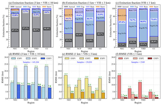
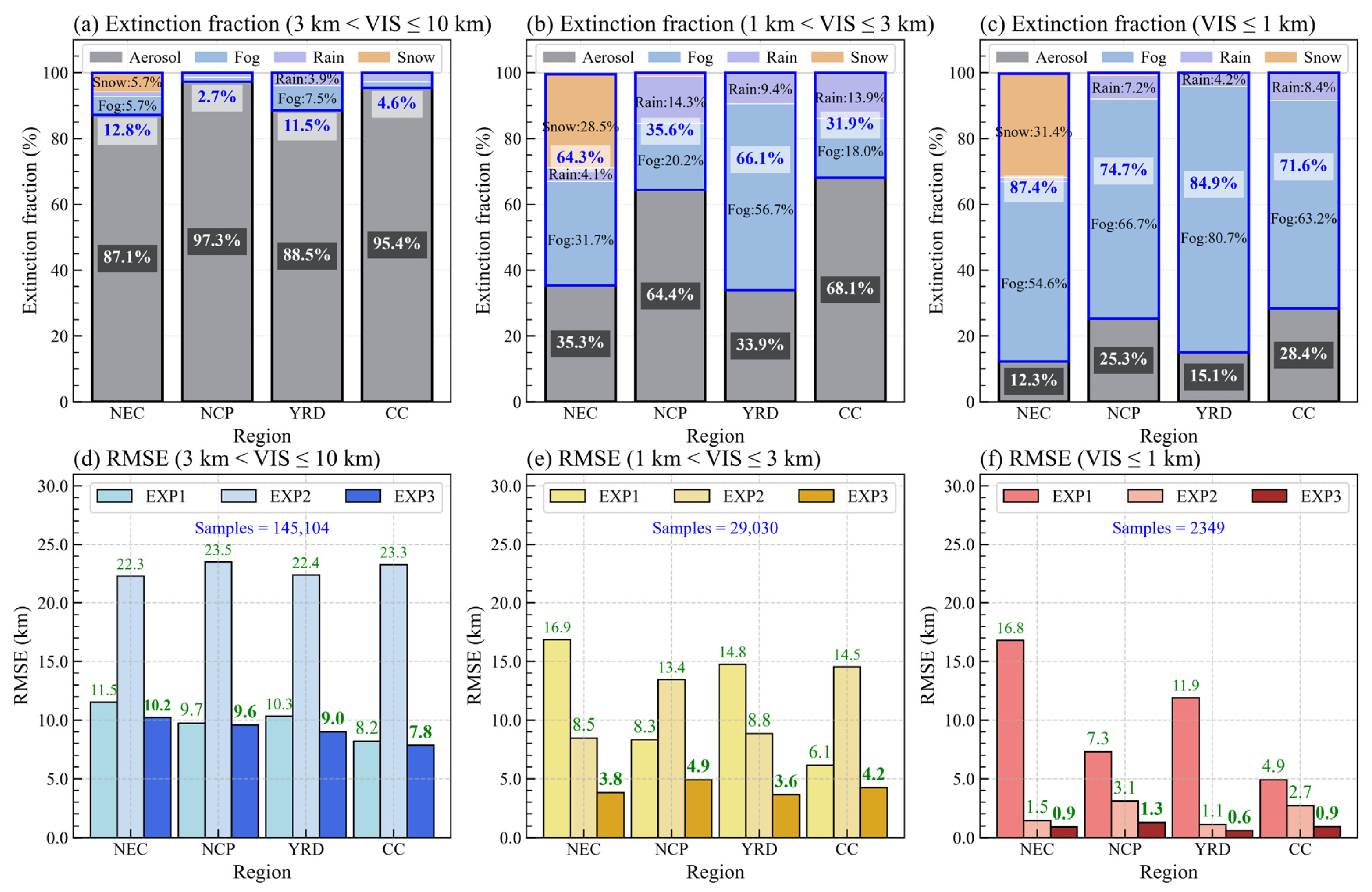
This section statistically evaluates the performance of EXP1, EXP2, and EXP3 and quantifies the model-estimated contributions of aerosol, fog, rain, and snow extinction for the full month. Figure 9 shows the mean model-estimated extinction contribution fractions in EXP3 (Figure 9a–c) and the regional mean RMSE of the three experiments (Figure 9d–f) for 3 < VIS ≤ 10 km, 1 < VIS ≤ 3 km, and VIS ≤ 1 km, with the RMSE computed on the same conditional samples. The grades are defined by the observed station-hour VIS, the same set of valid observation–simulation pairs is used for all three experiments, and the component fractions are the arithmetic mean of the individual sample fractions with equal weighting.

Figure 9. (a–c) EXP3 modeled mean extinction-component fractions and (d–f) regional mean RMSE of EXP1, EXP2, and EXP3 for three visibility grades (3 < VIS ≤ 10 km, 1 < VIS ≤ 3 km, and VIS ≤ 1 km) over Northeast China (NEC), the North China Plain (NCP), the Yangtze River Delta (YRD), and Central China (CC). The component fractions are the arithmetic mean of individual sample fractions, with all samples equally weighted. The total number of valid samples and contributing stations for each VIS grade are annotated in panels (d–f).

For 3 < VIS ≤ 10 km, aerosol extinction contributes 87.1–97.3% of the model-estimated total extinction in all four subregions, with hydrometeor contributions of 2.7–12.8% (Figure 9a). The hydrometeor contribution is largest in the NEC (12.8%), with comparable contributions from fog (5.7%) and snow (5.7%), followed by the YRD (11.5%), consisting mainly of fog (7.5%) and rain (3.9%). The smaller hydrometeor fractions in the CC (4.6%) and NCP (2.7%) are mainly from rain. EXP2 shows much higher RMSE (22.3–23.5 km) than EXP1 (8.2–11.5 km), and EXP3 reduces the regional mean RMSE relative to EXP1 by 1.0–12.6%, with the largest reductions in the NEC and the YRD, where the hydrometeor contributions are largest (Figure 9d). Aerosol extinction alone outperforms hydrometeor extinction alone for the 3–10 km VIS grade, and the combined extinction achieves the best overall performance.

For 1 < VIS ≤ 3 km, aerosol extinction contributes 33.9–68.1% and hydrometeor extinction contributes 31.9–66.1% of the model-estimated total extinction (Figure 9b). Fog dominates in the YRD (56.7%), NCP (20.2%), and CC (18.0%), and rain contributes 9.4%, 14.3%, and 13.9%, respectively. The NEC shows comparable fog (31.7%) and snow (28.5%) contributions. EXP2 outperforms EXP1 in the NEC and YRD, reflecting the large hydrometeor contribution in these two regions, but it remains clearly worse than EXP3 (3.6–4.9 km) because the aerosol contribution is not considered in EXP2. For NCP and CC, where aerosols contribute the most extinction, EXP1 shows better performance than EXP2. Correspondingly, EXP3 reduces the regional mean RMSE by 31.1–77.5% relative to EXP1 in all four subregions (Figure 9e).

For VIS ≤ 1 km, hydrometeors contribute 71.6–87.4% of the model-estimated total extinction in all four subregions and aerosols contribute 12.3–28.4% (Figure 9c). Fog is the largest contributor in the NEC (54.6%), NCP (66.7%), YRD (80.7%), and CC (63.2%), and rain contributes 7.2%, 4.2%, and 8.4% in the NCP, YRD, and CC, respectively; snow contributes 31.4% in the NEC. EXP2 achieves an RMSE of 1.1–3.1 km, compared with 4.9–16.8 km for EXP1 and 0.6–1.3 km for EXP3 (Figure 9f). Relative to EXP1, EXP3 reduces the RMSE by 94.6%, 82.2%, 95.0%, and 81.6% in the NEC, NCP, YRD, and CC, respectively. Hydrometeor extinction dominates the occurrence of extremely low VIS, and aerosol extinction remains an important contributor to total extinction.

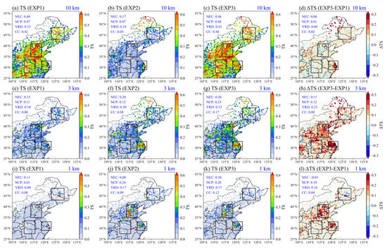
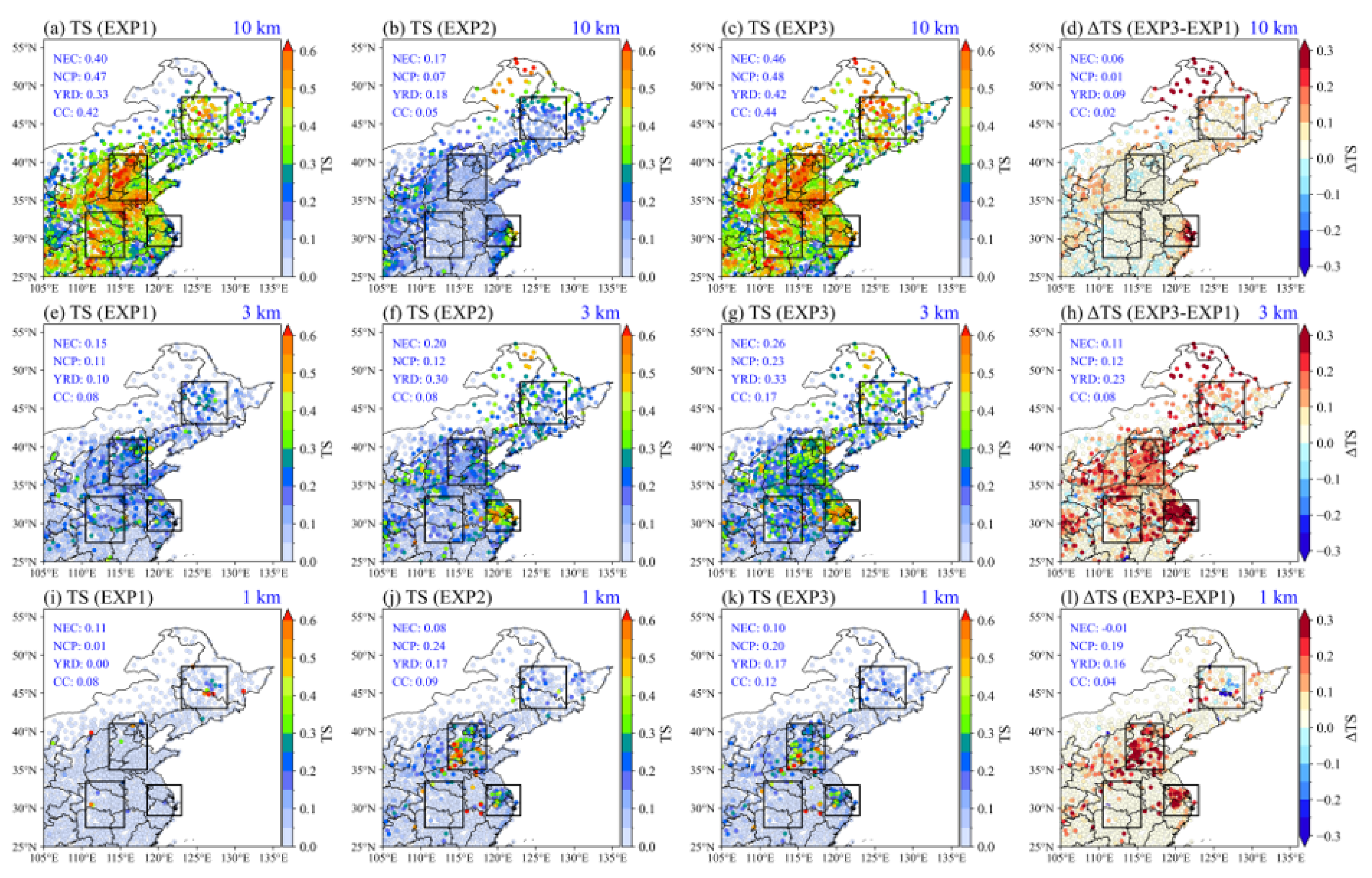
Figure 10 compares threat scores (TS) of the three experiments for 10, 3, and 1 km VIS levels. For 10 km VIS level, EXP1 achieves regional TS of 0.33–0.47, compared with 0.05–0.18 for EXP2. EXP3 shows regional TS of 0.42–0.48, with differences from EXP1 of 0.01–0.09, indicating that the occurrence of low VIS (≤10 km) is primarily determined by aerosol extinction. For 3 km VIS level, EXP1 shows regional TS of 0.08–0.15 and EXP2 shows TS of 0.08–0.30. EXP3 shows TS of 0.17–0.33, exceeding both EXP1 and EXP2 in every region, with differences from EXP1 ranging from 0.08 to 0.23; the largest difference occurs in the YRD, consistent with the large hydrometeor contribution identified in Figure 9b.

Figure 10. Threat score (TS) for (a–d) 10 km, (e–h) 3 km, and (i–l) 1 km VIS levels: (a,e,i) EXP1, (b,f,j) EXP2, (c,g,k) EXP3, and (d,h,l) the TS difference (ΔTS) between EXP3 and EXP1. Dots indicate observation sites, boxes denote the evaluation regions, and regional mean values are annotated in each panel.

For 1 km VIS level, EXP1 shows very limited capability in the four regions (regional TS of only 0.00–0.11). EXP2 achieves markedly higher TS in the NCP (0.24) and YRD (0.17), and EXP3 remains close to EXP2 there (0.20 and 0.17). EXP3 is therefore higher than EXP1 in the NCP, YRD, and CC, but only marginally lower than EXP1 in the NEC (0.10 versus 0.11). Relative to EXP2, EXP3 is slightly lower in the NCP (0.20 versus 0.24). These differences indicate that directly adding the two extinction components retains uncertainty where the modeled fog or precipitation is excessive or displaced, because the added aerosol extinction can further increase an already overestimated total extinction.

These results also define the limits of the three extinction calculations. First, the component fractions reported above are model estimates that depend on the adopted extinction parameterizations; the component partitioning may be subject to compensating biases not reflected in the total-extinction evaluation, and independent observations are therefore needed in future work to validate the estimated contributions. Second, the combined extinction is based on the independent-scattering approximation and uses activation thresholds for fog extinction, which may introduce additional uncertainty under compound conditions involving both high aerosol loading and dense fog. Third, the 0.1° grid cannot resolve every local fog or precipitation structure sampled by point observations. The lowest model level (~52 m) is well above the instrument level of surface stations: shallow radiation fog may occupy a layer thinner than, or sit below, the lowest model level, so the model may underestimate fog occurrence at valley and low-lying stations while overestimating it over grid-cell-averaged elevated terrain, as illustrated by fog observed at the summit of Mt. Oyama while a nearby lower-site instrument reported no fog [90]. Moreover, the 30-day November experiment samples haze, fog, rain, and snow but not their full seasonal cycle; warm-season convection, coastal sea fog, and deep-winter snowfall may alter the relative contributions of aerosol and hydrometeor extinction. Jointly considering aerosol and hydrometeor extinction offers a viable way forward for reliable compound low-visibility prediction; further work is needed to improve the predicted hydrometeor fields and the way the two extinction components are combined, particularly the treatment of aerosols activated into fog droplets.

4. Conclusions

Low VIS may involve aerosol pollution, fog, rain, and snow, or their combination across widespread regions, while VIS numerical predictions usually treat aerosol and hydrometeor extinction separately. The coupled chemistry–weather model GRAPES_Meso5.1/CUACE CW and surface meteorological observations are combined to investigate their relative contributions to atmospheric extinction and low-VIS prediction in eastern China. November 2024, which experiences several low-VIS events involving haze, fog, rain, and snow, is selected as the study period, and low VIS (≤10 km) is classified into three grades (3 < VIS ≤ 10 km, 1 < VIS ≤ 3 km, and VIS ≤ 1 km) for detailed discussion. Four key subregions and their representative cities, characterized by varying aerosol pollution and weather conditions, are focused on in this work. Firstly, the relationships between the graded low VIS and weather processes are analyzed based on observations. Three sensitivity experiments, EXP1 (aerosol extinction alone), EXP2 (hydrometeor extinction alone), and EXP3 (their combination), are then designed to calculate the extinction components separately and to predict VIS, and the simulated VIS is evaluated at regional and city scales and during several typical low-VIS episodes. Finally, the model-estimated relative contributions of aerosol and hydrometeor extinction to graded VIS are quantified, and RMSE for three VIS grades and TS for 10, 3, and 1 km VIS levels are adopted to evaluate the three experiments. The major conclusions are as follows:

Observations show that the weather processes associated with low VIS differ across VIS grades and among regions. For 3 < VIS ≤ 10 km, haze is the most frequent record in HRB and BJ in northern China, whereas fog prevails in SH and WH in southern China, and snow contributes to low VIS in HRB. For 1 < VIS ≤ 3 km, haze remains the most frequent record in HRB and BJ, whereas fog prevails in SH and WH; the haze fractions decrease compared with the 3–10 km grade in all four cities, while fog becomes more frequent in BJ and SH, and snow remains confined to HRB. For VIS ≤ 1 km, fog is the most frequent weather record in all four cities. Low VIS in the northern cities is more frequently associated with haze and snow, whereas that in the southern cities is more frequently associated with fog and rain, suggesting the necessity of incorporating multi-component extinction from aerosols and hydrometeors for low-VIS prediction across eastern China.

The sensitivity experiments show that the relative contributions of model-estimated aerosol and hydrometeor extinction differ across the graded VIS in different subregions. For 3 < VIS ≤ 10 km, aerosols contribute 87.1–97.3% of model-estimated total extinction in all four subregions, with comparable fog (5.7%) and snow (5.7%) contributions in the NEC; for 1 < VIS ≤ 3 km, aerosols contribute 33.9–68.1% and hydrometeors 31.9–66.1%, showing their comparable importance. Among the hydrometeors, fog contributes most in the YRD (56.7%), while the NEC shows comparable fog (31.7%) and snow (28.5%) contributions; for VIS ≤ 1 km, hydrometeors are the dominant contributors (71.6–87.4%), yet aerosols still yield appreciable contributions of 12.3–28.4% across the four subregions. Fog contributes 66.7%, 80.7%, and 63.2% to model-estimated total extinction in the NCP, YRD, and CC, with rain contributing 4.2–8.4%; in the NEC, fog contributes 54.6% and snow 31.4%. These results further show that neither aerosol nor hydrometeor extinction alone can explain low VIS, particularly at extremely low levels.

The extinction calculation jointly considering aerosol and hydrometeor extinction shows the overall best performance in low VIS prediction among the three sensitivity experiments, especially for VIS < 3 km and VIS ≤ 1 km. For 3 < VIS ≤ 10 km, the RMSE of the combined extinction (7.8–10.2 km) is lower than that of aerosol extinction (8.2–11.5 km) or hydrometeor extinction (22.3–23.5 km) alone; for 1 < VIS ≤ 3 km, the RMSE of the combined extinction is the lowest (3.6–4.9 km) among the three experiments; and for VIS ≤ 1 km, the RMSE of the combined extinction (0.6–1.3 km) is much lower than that of aerosol extinction (4.9–16.8 km) or hydrometeor extinction (1.1–3.1 km) alone. Similarly, for the 10 km VIS level, the TS of combined extinction (0.42–0.48) exceeds that of aerosol extinction (0.33–0.47) or hydrometeor extinction (0.05–0.18) alone; for the 3 km VIS level, the TS of combined extinction is the highest in all four subregions (0.17–0.33), versus 0.08–0.15 for aerosol extinction alone and 0.08–0.30 for hydrometeor extinction alone; and for the 1 km VIS level, the TS of combined extinction (0.10–0.20) is generally higher than those of aerosol or hydrometeor alone, particularly in the NCP and YRD.

The remaining uncertainties reflect both the extinction formulation itself and the modeled occurrence and distribution of fog and precipitation; the single-month period, the 95% RH cap on hygroscopic growth, and the bulk hydrometeor relations, together with the fog-versus-rain attribution under drizzle-containing conditions, also delimit the present conclusions. Multi-season evaluation, refined hydrometeor extinction parameterizations, and direct validation of the near-surface cloud-water and droplet-number fields are the next steps toward reliable compound low-VIS prediction.

References

- Gultepe, I. A review on weather impact on aviation operations: Visibility, wind, precipitation, icing. J. Airl. Oper. Aviat. Manag. 2023, 2, 1–44. [Google Scholar] [CrossRef] [Scilit]
- Yu, J.; Wang, Y.; Liu, M. Mechanisms of an extreme fog and haze event in the megacities of central and eastern China. Meteorol. Atmos. Phys. 2021, 133, 123–139. [Google Scholar] [CrossRef] [Scilit]
- Jia, X.; Quan, J.; Zheng, Z.; Liu, X.; Liu, Q.; He, H.; Liu, Y. Impacts of anthropogenic aerosols on fog in North China Plain. J. Geophys. Res. Atmos. 2019, 124, 252–265. [Google Scholar] [CrossRef] [Scilit]
- Li, Z.; Guo, J.; Ding, A.; Liao, H.; Liu, J.; Sun, Y.; Wang, T.; Xue, H.; Zhang, H.; Zhu, B. Aerosol and boundary-layer interactions and impact on air quality. Natl. Sci. Rev. 2017, 4, 810–833. [Google Scholar] [CrossRef] [Scilit]
- Niu, S.; Lu, C.; Yu, H.; Zhao, L.; Lü, J. Fog research in China: An overview. Adv. Atmos. Sci. 2010, 27, 639–662. [Google Scholar] [CrossRef] [Scilit]
- Kaskaoutis, D.G.; Kumar, S.; Sharma, D.; Singh, R.P.; Kharol, S.K.; Sharma, M.; Singh, A.K.; Singh, S.; Singh, A.; Singh, D. Effects of crop residue burning on aerosol properties, plume characteristics, and long-range transport over northern India. J. Geophys. Res. Atmos. 2014, 119, 5424–5444. [Google Scholar] [CrossRef] [Scilit]
- Sarkar, S.; Singh, R.P.; Chauhan, A. Crop residue burning in northern India: Increasing threat to Greater India. J. Geophys. Res. Atmos. 2018, 123, 6920–6934. [Google Scholar] [CrossRef] [Scilit]
- Chauhan, A.; Singh, R.P. Poor air quality and dense haze/smog during 2016 in the Indo-Gangetic plains associated with the crop residue burning and Diwali festival. In 2017 IEEE IGARSS; IEEE: Fort Worth, TX, USA, 2017; pp. 6048–6051. [Google Scholar] [CrossRef] [Scilit]
- Singh, R.P.; Kaskaoutis, D.G. Crop residue burning: A threat to South Asian air quality. Eos Trans. AGU 2014, 95, 333–334. [Google Scholar] [CrossRef] [Scilit]
- Wang, X.; Zhang, R.; Yu, W. The effects of PM2.5 concentrations and relative humidity on atmospheric visibility in Beijing. J. Geophys. Res. Atmos. 2019, 124, 2235–2259. [Google Scholar] [CrossRef] [Scilit]
- Yao, L.; Kong, S.; Zheng, H.; Chen, N.; Zhu, B.; Xu, K.; Cao, W.; Zhang, Y.; Zheng, M.; Cheng, Y.; et al. Co-benefits of reducing PM2.5 and improving visibility by COVID-19 lockdown in Wuhan. npj Clim. Atmos. Sci. 2021, 4, 40. [Google Scholar] [CrossRef] [Scilit]
- Ting, Y.C.; Young, L.H.; Lin, T.H.; Tsay, S.C.; Chang, K.E.; Hsiao, T.C. Quantifying the impacts of PM2.5 constituents and relative humidity on visibility impairment in a suburban area of eastern Asia using long-term in-situ measurements. Sci. Total Environ. 2022, 818, 151759. [Google Scholar] [CrossRef] [Scilit]
- Boudala, F.S.; Isaac, G.A. Parameterization of visibility in snow: Application in numerical weather prediction models. J. Geophys. Res. Atmos. 2009, 114, D19202. [Google Scholar] [CrossRef] [Scilit]
- Nelli, N.; Francis, D.; Abida, R.; Fonseca, R.; Masson, O.; Bosc, E. In-situ measurements of fog microphysics: Visibility parameterization and estimation of fog droplet sedimentation velocity. Atmos. Res. 2024, 309, 107570. [Google Scholar] [CrossRef] [Scilit]
- Singh, M.K.; Gautam, R. Developing a long-term high-resolution winter fog climatology over South Asia using satellite observations from 2002 to 2020. Remote Sens. Environ. 2022, 279, 113128. [Google Scholar] [CrossRef] [Scilit]
- Lyu, R.; Gao, W.; Peng, Y.; Qian, Y.; He, Q.; Cheng, T.; Yu, X.; Zhao, G. Fog–haze transition and drivers in the coastal region of the Yangtze River Delta. Int. J. Environ. Res. Public Health 2022, 19, 9608. [Google Scholar] [CrossRef] [Scilit]
- Eck, T.F.; Holben, B.N.; Reid, J.S.; Giles, D.M.; Rivas, M.A.; Singh, R.P.; Tripathi, S.N.; Bruegge, C.J.; Platnick, S.; Arnold, G.T.; et al. Fog- and cloud-induced aerosol modification observed by the Aerosol Robotic Network (AERONET). J. Geophys. Res. 2012, 117, D07206. [Google Scholar] [CrossRef] [Scilit]
- Gautam, R.; Hsu, N.C.; Kafatos, M.; Tsay, S.-C. Influences of winter haze on fog/low cloud over the Indo-Gangetic plains. J. Geophys. Res. Atmos. 2007, 112, D05207. [Google Scholar] [CrossRef] [Scilit]
- Gao, Y.; Zhang, M.; Liu, Z.; Wang, L.; Wang, P.; Xia, X.; Tao, M.; Zhu, L. Modeling the feedback between aerosol and meteorological variables in the atmospheric boundary layer during a severe fog–haze event over the North China Plain. Atmos. Chem. Phys. 2015, 15, 4279–4295. [Google Scholar] [CrossRef] [Scilit]
- Han, X.; Zhang, M.; Tao, J.; Wang, L.; Gao, J.; Wang, S.; Chai, F. Modeling aerosol impacts on atmospheric visibility in Beijing with RAMS-CMAQ. Atmos. Environ. 2013, 72, 177–191. [Google Scholar] [CrossRef] [Scilit]
- Peng, Y.; Wang, H.; Hou, M.; Jiang, T.; Zhang, M.; Zhao, T.; Che, H. Improved method of visibility parameterization focusing on high humidity and aerosol concentrations during fog–haze events: Application in the GRAPES_CUACE model in Jing-Jin-Ji, China. Atmos. Environ. 2020, 222, 117139. [Google Scholar] [CrossRef] [Scilit]
- Li, X.; Huang, L.; Li, J.; Shi, Z.; Wang, Y.; Zhang, H.; Ying, Q.; Yu, X.; Liao, H.; Hu, J. Source contributions to poor atmospheric visibility in China. Resour. Conserv. Recycl. 2019, 143, 167–177. [Google Scholar] [CrossRef] [Scilit]
- Liu, J.; Ren, C.; Huang, X.; Nie, W.; Wang, J.; Sun, P.; Chi, X.; Ding, A. Increased aerosol extinction efficiency hinders visibility improvement in eastern China. Geophys. Res. Lett. 2020, 47, e2020GL090167. [Google Scholar] [CrossRef] [Scilit]
- Xu, L.; Peng, Y.; Ram, K.; Zhang, Y.; Bao, M.; Wei, J. Investigation of the uncertainties of simulated optical properties of brown carbon at two Asian sites using a modified bulk aerosol optical scheme of the Community Atmospheric Model version 5.3. J. Geophys. Res. Atmos. 2021, 126, e2020JD033942. [Google Scholar] [CrossRef] [Scilit]
- Liu, Z.; Wang, H.; Peng, Y.; Zhang, W.; Zhao, M. Multiple regression analysis of low visibility focusing on severe haze-fog pollution in various regions of China. Atmosphere 2022, 13, 203. [Google Scholar] [CrossRef] [Scilit]
- Shen, X.; Sun, J.; Zhang, X.; Wang, H.; Zhou, C.; Zhang, Y.; Zhong, J.; Liu, Z.; Xia, C.; Hu, X.; et al. A novel method of retrieving low visibility during heavily polluted episodes in the North China plain. Atmos. Environ. X 2021, 9, 100101. [Google Scholar] [CrossRef] [Scilit]
- Mie, G. Beiträge zur Optik trüber Medien, speziell kolloidaler Metallösungen. Ann. Phys. 1908, 330, 377–445. [Google Scholar] [CrossRef] [Scilit]
- Zou, J.; Yang, S.; Hu, B.; Liu, Z.; Gao, W.; Xu, H.; Du, C.; Wei, J.; Ma, Y.; Ji, D.; et al. A closure study of aerosol optical properties as a function of RH using a κ-AMS-BC-Mie model in Beijing, China. Atmos. Environ. 2019, 197, 1–13. [Google Scholar] [CrossRef] [Scilit]
- Malm, W.C.; Sisler, J.F.; Huffman, D.; Eldred, R.A.; Cahill, T.A. Spatial and seasonal trends in particle concentration and optical extinction in the United States. J. Geophys. Res. Atmos. 1994, 99, 1347–1370. [Google Scholar] [CrossRef] [Scilit]
- Pitchford, M.; Malm, W.; Schichtel, B.; Kumar, N.; Lowenthal, D.; Hand, J. Revised algorithm for estimating light extinction from IMPROVE particle speciation data. J. Air Waste Manag. Assoc. 2007, 57, 1326–1336. [Google Scholar] [CrossRef] [Scilit]
- Jiang, L.; Zhang, Z.; Zhu, B.; Shen, Y.; Wang, H.; Shi, S.; Sha, D. Comparison of parameterizations for the atmospheric extinction coefficient in Lin’an, China. Sci. Total Environ. 2018, 621, 507–515. [Google Scholar] [CrossRef] [Scilit]
- Khanna, I.; Khare, M.; Gargava, P.; Khan, A.A. Effect of PM2.5 chemical constituents on atmospheric visibility impairment. J. Air Waste Manag. Assoc. 2018, 68, 430–437. [Google Scholar] [CrossRef] [Scilit]
- Huang, H.; Zhang, G. Case studies of low-visibility forecasting in falling snow with WRF model. J. Geophys. Res. Atmos. 2017, 122, 12862–12874. [Google Scholar] [CrossRef] [Scilit]
- Lin, C.; Zhang, Z.; Pu, Z.; Wang, F. Numerical simulations of an advection fog event over Shanghai Pudong International Airport with the WRF model. J. Meteorol. Res. 2017, 31, 874–889. [Google Scholar] [CrossRef] [Scilit]
- Gultepe, I.; Fernando, H.J.S.; Pardyjak, E.R.; Hoch, S.W.; Silver, Z.; Creegan, E.; Leo, L.S.; Pu, Z.; De Wekker, S.F.J.; Hang, C. An overview of the MATERHORN fog project: Observations and predictability. Pure Appl. Geophys. 2016, 173, 2983–3010. [Google Scholar] [CrossRef] [Scilit]
- Kunkel, B.A. Parameterization of droplet terminal velocity and extinction coefficient in fog models. J. Appl. Meteorol. Climatol. 1984, 23, 34–41. [Google Scholar] [CrossRef] [Scilit]
- Gultepe, I.; Müller, M.D.; Boybeyi, Z. A new visibility parameterization for warm-fog applications in numerical weather prediction models. J. Appl. Meteorol. Climatol. 2006, 45, 1469–1480. [Google Scholar] [CrossRef] [Scilit]
- Gultepe, I.; Tardif, R.; Michaelides, S.C.; Cermak, J.; Bott, A.; Bendix, J.; Müller, M.D.; Pagowski, M.; Hansen, B.; Ellrod, G.; et al. Fog research: A review of past achievements and future perspectives. Pure Appl. Geophys. 2007, 164, 1121–1159. [Google Scholar] [CrossRef] [Scilit]
- Gultepe, I.; Pearson, G.; Milbrandt, J.A.; Hansen, B.; Platnick, S.; Taylor, P.; Gordon, M.; Oakley, J.P.; Cober, S.G. The fog remote sensing and modeling field project. Bull. Am. Meteorol. Soc. 2009, 90, 341–360. [Google Scholar] [CrossRef] [Scilit]
- Song, J.I.; Yum, S.S.; Gultepe, I.; Chang, K.-H.; Kim, B.-G. Development of a new visibility parameterization based on the measurement of fog microphysics at a mountain site in Korea. Atmos. Res. 2019, 229, 115–126. [Google Scholar] [CrossRef] [Scilit]
- Gultepe, I.; Milbrandt, J.A. Probabilistic parameterizations of visibility using observations of rain precipitation rate, relative humidity, and visibility. J. Appl. Meteorol. Climatol. 2010, 49, 36–46. [Google Scholar] [CrossRef] [Scilit]
- Stoelinga, M.T.; Warner, T.T. Nonhydrostatic, mesobeta-scale model simulations of cloud ceiling and visibility for an East Coast winter precipitation event. J. Appl. Meteorol. Climatol. 1999, 38, 385–404. [Google Scholar] [CrossRef] [Scilit]
- Wang, H.; Zhang, X.Y.; Wang, P.; Peng, Y.; Zhang, W.J.; Liu, Z.D.; Han, C.; Li, S.T.; Wang, Y.Q.; Che, H.Z.; et al. Chemistry-weather interacted model system GRAPES_Meso5.1/CUACE CW v1.0: Development, evaluation and application in better haze/fog prediction in China. J. Adv. Model. Earth Syst. 2022, 14, e2022MS003222. [Google Scholar] [CrossRef] [Scilit]
- Xie, Y.; Wang, X.; Gao, Y.; Chen, B.; van der A, R.; Ding, J.; Gu, W.; Zhou, M.; Wang, H. Improving visibility forecasting during haze-fog processes in Shanghai and eastern China: The significance of aerosol and hydrometeor extinction. Atmos. Environ. 2024, 337, 120756. [Google Scholar] [CrossRef] [Scilit]
- Han, C.; Wang, H.; Peng, Y.; Liu, Z.; Zhang, W.; Zhao, Y.; Ning, H.; Wang, P.; Che, H. The application study of the revised IMPROVE atmospheric extinction algorithm in atmospheric chemistry model focusing on improving low visibility prediction in eastern China. Atmos. Res. 2024, 298, 107135. [Google Scholar] [CrossRef] [Scilit]
- Liu, Z.; Wang, H.; Zhang, L.; Zhou, Y.; Zhang, W.; Peng, Y.; Zhang, Y.; Che, H.; Zhao, M.; Hu, J.; et al. Incorporation and improvement of a heterogeneous chemistry mechanism in the atmospheric chemistry model GRAPES_Meso5.1/CUACE and its impacts on secondary inorganic aerosol and PM2.5 simulations in Middle-Eastern China. Sci. Total Environ. 2022, 847, 157530. [Google Scholar] [CrossRef] [Scilit]
- Ning, H.; Wang, H.; Liu, Z.; Peng, Y.; Zhang, W.; Han, C.; Zhao, Y.; Wang, P.; Gui, H.; Wang, J.; et al. Study on the Contribution of the Major Desert Groups on SDS Weather in East Asia Combining the Model Simulation and Multiple Observations. Atmos. Res. 2025, 317, 107967. [Google Scholar] [CrossRef] [Scilit]
- Peng, Y.; Wang, H.; Zhang, X.; Zheng, Y.; Zhang, X.; Zhang, W.; Liu, Z.; Gui, K.; Liu, H.; Wang, Y.; et al. Aerosol-radiation interaction in the operational atmospheric chemistry model GRAPES_Meso5.1/CUACE and its impacts on mesoscale NWP in Beijing-Tianjin-Hebei, China. Atmos. Res. 2022, 280, 106402. [Google Scholar] [CrossRef] [Scilit]
- Peng, Y.; Wang, H.; Zhang, X.; Liu, Z.; Zhang, W.; Li, S.; Han, C.; Che, H. Superimposed effects of typical local circulations driven by mountainous topography and aerosol–radiation interaction on heavy haze in the Beijing–Tianjin–Hebei central and southern plains in winter. Atmos. Chem. Phys. 2023, 23, 8325–8339. [Google Scholar] [CrossRef] [Scilit]
- Zhang, W.; Zhang, X.; Wang, H. The role of aerosol-radiation interaction in the meteorology prediction at the weather scale in the numerical weather prediction model. Geophys. Res. Lett. 2022, 49, e2021GL097026. [Google Scholar] [CrossRef] [Scilit]
- Zhang, W.; Wang, H.; Zhang, X.; Huang, L.; Peng, Y.; Liu, Z.; Zhang, X.; Che, H. Aerosol–cloud interaction in the atmospheric chemistry model GRAPES_Meso5.1/CUACE and its impacts on mesoscale numerical weather prediction under haze pollution conditions in Jing–Jin–Ji in China. Atmos. Chem. Phys. 2022, 22, 15207–15221. [Google Scholar] [CrossRef] [Scilit]
- Chen, D.; Xue, J.; Yang, X.; Zhang, H.; Shen, X.; Hu, J.; Wang, Y.; Ji, L.; Chen, J. New generation of multi-scale NWP system (GRAPES): General scientific design. Chin. Sci. Bull. 2008, 53, 3433–3445. [Google Scholar] [CrossRef] [Scilit]
- Zhang, R.; Shen, X. On the development of the GRAPES—A new generation of the national operational NWP system in China. Chin. Sci. Bull. 2008, 53, 3429–3432. [Google Scholar] [CrossRef] [Scilit]
- Xu, G.; Chen, D.; Xue, J.; Sun, J.; Shen, X.; Shen, Y.; Huang, L.; Wu, X.; Zhang, H.; Wang, S. The program structure designing and optimizing tests of GRAPES physics. Chin. Sci. Bull. 2008, 53, 3470–3476. [Google Scholar] [CrossRef] [Scilit]
- Thompson, G.; Field, P.R.; Rasmussen, R.M.; Hall, W.D. Explicit forecasts of winter precipitation using an improved bulk microphysics scheme. Part II: Implementation of a new snow parameterization. Mon. Weather Rev. 2008, 136, 5095–5115. [Google Scholar] [CrossRef] [Scilit]
- Gong, S.L.; Zhang, X.Y. CUACE/Dust—An integrated system of observation and modeling systems for operational dust forecasting in Asia. Atmos. Chem. Phys. 2008, 8, 2333–2340. [Google Scholar] [CrossRef] [Scilit]
- Gong, S.L.; Barrie, L.A.; Blanchet, J.P.; von Salzen, K.; Lohmann, U.; Lesins, G.; Spacek, L.; Zhang, L.M.; Girard, E.; Lin, H.; et al. Canadian Aerosol Module: A size-segregated simulation of atmospheric aerosol processes for climate and air quality models 1. Module development. J. Geophys. Res. Atmos. 2003, 108, AAC 3-1–AAC 3-16. [Google Scholar] [CrossRef] [Scilit]
- Sarwar, G.; Luecken, D.; Yarwood, G. Developing and implementing an updated chlorine chemistry into the community multiscale air quality model. In Developments in Environmental Science; Borrego, C., Renner, E., Eds.; Elsevier: Amsterdam, The Netherlands, 2007; pp. 168–176. [Google Scholar] [CrossRef] [Scilit]
- Fountoukis, C.; Nenes, A. ISORROPIA II: A computationally efficient thermodynamic equilibrium model for K+–Ca2+–Mg2+–NH4+–Na+–SO42−–NO3−–Cl−–H2O aerosols. Atmos. Chem. Phys. 2007, 7, 4639–4659. [Google Scholar] [CrossRef] [Scilit]
- Shen, X.; Wang, M.; Xiao, F. A study of the high-order accuracy and positive definite conformal advection scheme in the GRAPES model I: Scientific design and idealized tests. Acta Meteorol. Sin. 2011, 69, 1–15. [Google Scholar] [CrossRef]
- Kain, J.S. The Kain–Fritsch convective parameterization: An update. J. Appl. Meteorol. 2004, 43, 170–181. [Google Scholar] [CrossRef] [Scilit]
- Chou, M.-D.; Suarez, M.; Liang, X.-Z.; Yan, M.; Cote, C. A Thermal Infrared Radiation Parameterization for Atmospheric Studies; NASA/TM-2001-104606; NASA Technical Memorandum: Hampton, VA, USA, 2001; Volume 19, p. 54. [Google Scholar]
- Price, E.; Mielikainen, J.; Huang, M.; Huang, B.; Huang, H.L.A.; Lee, T. GPU-accelerated longwave radiation scheme of the Rapid Radiative Transfer Model for General Circulation Models (RRTMG). IEEE J. Sel. Top. Appl. Earth Obs. Remote Sens. 2014, 7, 3660–3667. [Google Scholar] [CrossRef] [Scilit]
- Pleim, J.E. A simple, efficient solution of flux–profile relationships in the atmospheric surface layer. J. Appl. Meteorol. Climatol. 2006, 45, 341–347. [Google Scholar] [CrossRef] [Scilit]
- Hong, S.Y.; Pan, H.L. Nonlocal boundary layer vertical diffusion in a medium-range forecast model. Mon. Weather Rev. 1996, 124, 2322–2339. [Google Scholar] [CrossRef] [Scilit]
- Ek, M.B.; Mitchell, K.E.; Lin, Y.; Rogers, E.; Grunmann, P.; Koren, V.; Gayno, G.; Tarpley, J.D. Implementation of Noah land surface model advances in the National Centers for Environmental Prediction operational mesoscale Eta model. J. Geophys. Res. Atmos. 2003, 108, 8851. [Google Scholar] [CrossRef] [Scilit]
- Koschmieder, H. Theorie der horizontalen Sichtweite. In Die Sichtweite im Nebel und die Möglichkeiten Ihrer Künstlichen Beeinflussung; VS Verlag für Sozialwissenschaften: Wiesbaden, Germany, 1924; Volume 12, pp. 33–53. [Google Scholar]
- Thompson, G.; Eidhammer, T. A study of aerosol impacts on clouds and precipitation development in a large winter cyclone. J. Atmos. Sci. 2014, 71, 3636–3658. [Google Scholar] [CrossRef] [Scilit]
- Feingold, G.; Heymsfield, A.J. Parameterizations of condensational growth of droplets for use in general circulation models and cloud models. J. Atmos. Sci. 1992, 49, 2325–2343. [Google Scholar] [CrossRef] [Scilit]
- Van de Hulst, H.C. Light Scattering by Small Particles; Dover Publications: New York, NY, USA, 1981. [Google Scholar]
- Zhou, B.; Du, J.; Gultepe, I.; Dimego, G. Forecast of low visibility and fog from NCEP: Current status and efforts. Pure Appl. Geophys. 2012, 169, 895–909. [Google Scholar] [CrossRef] [Scilit]
- Zheng, B.; Tong, D.; Li, M.; Liu, F.; Hong, C.; Geng, G.; Li, H.; Li, X.; Peng, L.; Qi, J.; et al. Trends in China’s anthropogenic emissions since 2010 as the consequence of clean air actions. Atmos. Chem. Phys. 2018, 18, 14095–14111. [Google Scholar] [CrossRef] [Scilit]
- Wang, H.; Xue, M.; Zhang, X.Y.; Liu, H.L.; Zhou, C.H.; Tan, S.C.; Che, H.Z.; Chen, B.; Li, T. Mesoscale modeling study of the interactions between aerosols and PBL meteorology during a haze episode in Jing–Jin–Ji (China) and its nearby surrounding region—Part 1: Aerosol distributions and meteorological features. Atmos. Chem. Phys. 2015, 15, 3257–3275. [Google Scholar] [CrossRef] [Scilit]
- Zeng, Z.; Gui, K.; Wang, Z.; Luo, M.; Geng, H.; Ge, E.; An, J.; Song, X.; Ning, G.; Zhai, S.; et al. Estimating hourly surface PM2.5 concentrations across China from high-density meteorological observations by machine learning. Atmos. Res. 2021, 254, 105516. [Google Scholar] [CrossRef] [Scilit]
- Zhang, X.; Gui, K.; Zeng, Z.; Fei, Y.; Li, L.; Zheng, Y.; Peng, Y.; Liu, Y.; Shang, N.; Zhao, H.; et al. Mapping the seamless hourly surface visibility in China: A real-time retrieval framework using a machine-learning-based stacked ensemble model. npj Clim. Atmos. Sci. 2024, 7, 68. [Google Scholar] [CrossRef] [Scilit]
- Zhong, J.; Zhang, X.; Gui, K.; Wang, Y.; Che, H.; Shen, X.; Zhang, L.; Zhang, Y.; Sun, J.; Zhang, W. Robust prediction of hourly PM2.5 from meteorological data using LightGBM. Natl. Sci. Rev. 2021, 8, nwaa307. [Google Scholar] [CrossRef] [Scilit]
- World Meteorological Organization (WMO). Guide to Instruments and Methods of Observation (WMO-No. 8); WMO: Geneva, Switzerland, 2024; Volume I, Chapter 9; Available online: https://library.wmo.int/idurl/4/68695 (accessed on 4 May 2026).
- Wang, Z.; Huang, X.; Ma, S. Atmospheric Detection; China Meteorological Press: Beijing, China, 2011; pp. 41–42. (In Chinese) [Google Scholar]
- Lyu, R.; Wang, Y.; Peng, Y.; Gao, W.; Yang, H.; Tan, X.; He, Q.; Cheng, T.; Zhang, R. Long-term variation characteristics and influencing factors of low-visibility events on the coast of China. Atmos. Res. 2021, 257, 105583. [Google Scholar] [CrossRef] [Scilit]
- Hao, Y.; Gou, Y.; Wang, Z.; Huang, W.; Wan, F.; Tian, M.; Chen, J. Current challenges in the visibility improvement of urban Chongqing in Southwest China: From the perspective of PM2.5-bound water uptake property over 2015–2021. Atmos. Res. 2024, 300, 107215. [Google Scholar] [CrossRef] [Scilit]
- Lin, Y.; Huang, K.; Zhuang, G.; Fu, J.S.; Wang, Q.; Liu, T.; Deng, C.; Fu, Q. A multi-year evolution of aerosol chemistry impacting visibility and haze formation over an Eastern Asia megacity, Shanghai. Atmos. Environ. 2014, 92, 76–86. [Google Scholar] [CrossRef] [Scilit]
- Liu, X.; Gu, J.; Li, Y.; Cheng, Y.; Qu, Y.; Han, T.; Wang, J.; Tian, H.; Chen, J.; Zhang, Y. Increase of aerosol scattering by hygroscopic growth: Observation, modeling, and implications on visibility. Atmos. Res. 2013, 132, 91–101. [Google Scholar] [CrossRef] [Scilit]
- World Meteorological Organization (WMO). Manual on Codes (WMO-No. 306); WMO: Geneva, Switzerland, 2019; Volume I.1, Available online: https://library.wmo.int/idurl/4/35713 (accessed on 4 May 2026).
- Chen, J.; Zhao, C.S.; Ma, N.; Liu, P.F.; Göbel, T.; Hallbauer, E.; Deng, Z.Z.; Ran, L.; Xu, W.Y.; Liang, Z.; et al. A parameterization of low visibilities for hazy days in the North China Plain. Atmos. Chem. Phys. 2012, 12, 4935–4950. [Google Scholar] [CrossRef] [Scilit]
- Cheng, Z.; Wang, S.; Qiao, L.; Wang, H.; Zhou, M.; Fu, X.; Lou, S.; Luo, L.; Jiang, J.; Chen, C.; et al. Insights into extinction evolution during extreme low visibility events: Case study of Shanghai, China. Sci. Total Environ. 2018, 618, 793–803. [Google Scholar] [CrossRef] [Scilit]
- Wang, X.; Shen, X.J.; Sun, J.Y.; Zhang, X.Y.; Wang, Y.Q.; Zhang, Y.M.; Wang, P.; Xia, C.; Qi, X.F.; Zhong, J.T. Size-resolved hygroscopic behavior of atmospheric aerosols during heavy aerosol pollution episodes in Beijing in December 2016. Atmos. Environ. 2018, 194, 188–197. [Google Scholar] [CrossRef] [Scilit]
- Xue, B.; Kuang, Y.; Xu, W.; Zhao, P. Joint increase of aerosol scattering efficiency and aerosol hygroscopicity aggravate visibility impairment in the North China Plain. Sci. Total Environ. 2022, 839, 156279. [Google Scholar] [CrossRef] [Scilit]
- Tu, X.; Yao, R.; Hu, L.; Xu, D.; Yang, H. Observation and simulation study on the macro–microphysical characteristics of a coastal fog offshore Zhejiang Province of China. Atmos. Res. 2023, 282, 106537. [Google Scholar] [CrossRef] [Scilit]
- Igawa, M.; Wang, Y. Characteristics of fog and drizzle in Yokohama and in Mt. Oyama, Japan. Water Air Soil Pollut. 2022, 233, 533. [Google Scholar] [CrossRef] [Scilit]
- Wang, Y.; Okochi, H.; Igawa, M. Characteristics of fog and fog collection with passive collector at Mt. Oyama in Japan. Water Air Soil Pollut. 2021, 232, 260. [Google Scholar] [CrossRef] [Scilit]
Disclaimer/Publisher’s Note: The statements, opinions and data contained in all publications are solely those of the individual author(s) and contributor(s) and not of MDPI and/or the editor(s). MDPI and/or the editor(s) disclaim responsibility for any injury to people or property resulting from any ideas, methods, instructions or products referred to in the content. |
© 2026 by the authors. Licensee MDPI, Basel, Switzerland. This article is an open access article distributed under the terms and conditions of the Creative Commons Attribution (CC BY) license.