


Abstract
This study developed a machine-learning-based detection-alarm algorithm using hydrogen sulfide (H2S) and ammonia (NH3) as core chemical inputs to determine the analytical detection status of 20 odor compounds and evaluated its external applicability at an independent facility. Data collected at 20 min intervals from three odor-emitting facilities were used, with detection defined as a concentration at or above the compound-specific detection limit. Data from a livestock farm and a wastewater treatment facility were used to develop a meteorological–temporal baseline model (M0b) and an alarm model additionally incorporating H2S and NH3 (M4). Model selection, probability calibration, and compound-specific thresholds were determined using nested site–week cross-validation, and the finalized models were applied unchanged to Site C. In the development dataset, mean average precision (AP) increased from 0.362 for M0b to 0.463 for M4 (ΔAP = +0.101), with improvements for 17 of 20 compounds. At Site C, mean AP increased from 0.424 to 0.443 (ΔAP = +0.019), with improvements for 13 compounds. Excluding exploratory methyl isobutyl ketone, mean ΔAP was +0.106 and +0.020, respectively. External evaluation included only four calendar-week groups, yielding a minimum attainable two-sided permutation p-value of 0.125. No compound-specific improvement reached Benjamini–Hochberg-adjusted significance (q < 0.05) in either dataset; the external findings are therefore exploratory. Under fixed-threshold operation, dimethyl sulfide achieved a precision of 0.921 and a false-positive rate of 0.057, but recall was 0.182. These results suggest that H2S and NH3 may provide useful additional information for screening multiple odor compounds, while emphasizing the need for site-specific threshold assessment and further independent validation.
1. Introduction
Continuous monitoring of multiple odorants at odor-emitting facilities requires an observation system capable of distinguishing individual chemical species [1,2,3]. However, during long-term multi-component monitoring, it is difficult to obtain stable and simultaneous observations for all compounds because of analytical intervals, instrument downtime, and missing measurements [1,2,3]. To overcome these limitations, electronic noses and instrumental odor-monitoring technologies that combine sensor signals with multivariate algorithms have been investigated [1,2,3,4]. Previous studies conducted at wastewater treatment facilities and other odor sources have reported the classification of odor types and estimation of odor concentrations [5,6,7,8,9], as well as the real-time identification of emission peaks [10,11,12]. However, these prediction targets are distinct from determining whether individual odorants are analytically detected [6,7,8,9,10,11,12,13]. In particular, approaches that use a limited number of continuously measured signals to simultaneously assess the detectability of multiple individual odorants and translate these assessments into compound-specific alarms require further evaluation [13]. Therefore, establishing an alarm framework that uses continuously measurable representative chemical signals to screen the detection status of multiple odorants may provide a useful complementary tool for field monitoring.
Hydrogen sulfide (H2S) and ammonia (NH3) are representative gases routinely monitored at odor-emitting facilities, and commercially available sensors for these gases are readily accessible, making them suitable for continuous field measurements [14,15,16,17,18,19,20,21,22]. Both compounds have been widely managed as key monitoring parameters at various odor sources, including livestock facilities and wastewater treatment plants, and offer practical advantages as chemical signals for field applications [14,15,16,17,18,19,20,21,22,23,24]. Based on these characteristics, H2S and NH3 were considered as core chemical signals that may indirectly reflect multi-component odor conditions, and their continuous measurements were used to assess the detectability of the remaining odorants. Meteorological and temporal variables were additionally incorporated as supplementary information to account for variations associated with emission and dispersion conditions [15,18,25]. This approach was not intended to directly predict the concentrations of individual odorants, but rather to screen whether each compound was analytically detectable at the same observation time using a limited set of continuously measured signals. Accordingly, the proposed framework is not intended to directly replace costly multi-component chemical analyses, but rather to serve as a supplementary monitoring tool for prioritizing compounds that may require additional analysis or field response.
For multi-component detection alarms, it is necessary to consider not only the ranking performance of classification models but also their operational characteristics when model outputs are converted into practical alarms [26,27,28,29,30,31]. Average precision (AP) is useful for summarizing the precision–recall relationship in imbalanced binary classification [26,27,28,29] and can be used to compare classification performance across compounds with markedly different proportions of positive observations. However, a high AP does not necessarily indicate satisfactory performance under actual alarm operation, because the proportions of missed detections and false alarms can vary substantially depending on the selected decision threshold [30,31]. In odor monitoring, achieving an appropriate balance between sensitivity for capturing true detection states and selectivity for reducing unnecessary alarms is particularly important [26,27,28,29,30,31]. Therefore, evaluation of compound-specific detectability should consider ranking-based metrics such as AP together with operational metrics, including recall, precision, false-positive rate, and alarm frequency [26,27,28,29,30,31]. Such evaluation represents an important step in translating classification performance into a practically applicable alarm framework.
Environmental monitoring data often exhibit temporal and clustered dependence; therefore, evaluating model performance under new conditions is also important [32,33]. Internal evaluation using data from the same facilities may be affected by site-specific emission characteristics, operating conditions, and observation periods, and classification performance and alarm operating characteristics may change when these conditions differ [32,33]. In particular, odor-emitting facilities can differ in compound-specific detection frequencies and concentration distributions depending on facility type and process conditions [14,15,16,17,18,19,20,25]; therefore, internal cross-validation alone may be insufficient for assessing applicability to new facilities [32,33,34]. Accordingly, external evaluation using an independent facility is important for determining whether H2S and NH3 continue to provide additional classification information under new conditions and for examining how compound-specific alarm characteristics are maintained or altered [34]. Evaluating differences in performance and operating points at an external facility may also provide a basis for future site-specific threshold adjustment and the establishment of alarm operating criteria [30,31,34].
Accordingly, this study aimed to develop compound-specific detection-alarm algorithms for the remaining 20 odorants using H2S and NH3 as core chemical signals and to evaluate their applicability at an independent facility. Classification performance was compared between a baseline model using only meteorological and temporal information and an alarm model additionally incorporating H2S and NH3 to assess the incremental information provided by these two chemical signals. Compound-specific detection performance and alarm operating characteristics under fixed decision thresholds were then evaluated at the external facility. In addition, an independent facility excluded from model development was used for external evaluation to examine the applicability of the alarm framework established using the development data. The prediction target of this study was restricted to the analytical detection status of individual odorants at the same observation time, rather than future odor occurrence or odor concentration.
2. Materials and Methods
2.1. Study Design and Observational Data for the Detection-Alarm Algorithm
Odor and meteorological monitoring data recorded at 20 min intervals from 1 August 2022 to 30 June 2023 at a livestock farm, a wastewater treatment facility (WWTF), and Site C were used. The livestock farm and WWTF were used for model development, whereas Site C, an anonymized organic waste treatment facility described in our previous study [35], was used for independent external evaluation. This facility type differs from those of the two development sites. Differences in facility processes and emission sources may contribute to the observed differences in detection prevalence, although the present data do not establish their source-specific causes. Of the 22 odorants, H2S and NH3 were used as the core chemical inputs, and the remaining 20 compounds were treated as independent alarm targets. Concentrations of the target compounds were used only to generate training labels and evaluate model performance and were not included as predictive inputs. Inputs and labels were aligned at the same observation time, and no lagged variables or moving averages were used. Therefore, the present analysis evaluates detection alarms at the time of observation and does not represent predictive performance before an event occurs. This simultaneous-input design was adopted to evaluate the additional classification information provided by H2S and NH3 measured at the same observation time. Lagged inputs and moving averages were not evaluated, so the present results do not establish whether temporal features would improve classification or alarm stability. Future work should compare the current approach with models incorporating preceding observations and trailing-window summaries to assess potential benefits from temporal dependence and delayed responses. For real-time application, these features should use only information available at or before the alarm time.
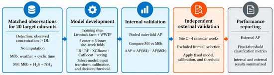
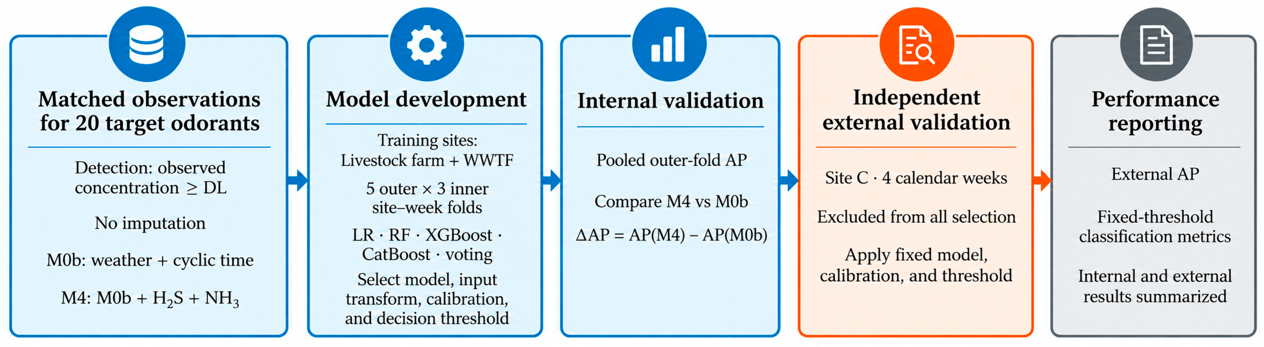
Figure 1 illustrates the development and external application procedures for the compound-specific alarm models. For each target compound, the candidate model and H2S–NH3 input transformation were selected, and out-of-fold prediction probabilities were used to determine probability calibration and the alarm threshold. After completion of the development procedure, the final model was refitted using the entire development dataset, and the model, input transformation, calibration function, and threshold were fixed before application to Site C. This separation of model selection from performance evaluation is intended to reduce optimistic performance estimates arising from the model-selection process and to assess generalization performance on independent data [34,35]. Target labels from Site C were not used to determine eligibility for model development, model type, hyperparameters, input transformation, probability calibration, or decision thresholds. For each target, M0b and M4 used the same observation rows and shared the same nested cross-validation splits.
Figure 1.
Study workflow for H2S- and NH3-based odor detection alarms. H2S, hydrogen sulfide; NH3, ammonia; DL, detection limit; WWTF, wastewater treatment facility; LR, logistic regression; RF, random forest; XGBoost 3.2.0, extreme gradient boosting; CatBoost 1.2.10, categorical boosting; AP, average precision.
2.2. Measurement Systems and Compound-Specific Detection Limits
The 22 odorants were measured using thermal-desorption gas chromatography with flame ionization detection (TD-GC-FID), thermal-desorption gas chromatography with photoionization detection (TD-GC-PID), and tunable diode laser spectroscopy (TDLS) (Table 1). The GC systems and TDLS instruments were manufactured by KNR Co., Ltd. (Seoul, Republic of Korea). Nineteen compounds, including aldehydes, volatile fatty acids, ketones, and aromatic compounds, were measured using TD-GC-FID, whereas H2S and methyl mercaptan were measured using TD-GC-PID. NH3 was measured directly using TDLS. The analytical systems and compound-specific detection limits were based on the measurement methods described in a previous study [35].
Table 1.
Measurement systems, detection limits, and their roles in the present study.
Compound-specific detection limits for TD-GC-FID ranged from 0.21 to 1.66 ppb, whereas those for TD-GC-PID were 0.35 ppb for methyl mercaptan and 0.62 ppb for H2S. The detection limit for NH3 was 0.10 ppm, corresponding to 100 ppb. Detection limits for all 20 target compounds classified in this study are reported in ppb (Table A1). H2S and NH3 were used as continuous inputs and were not converted into separate binary variables based on their respective detection limits. The detection limit (DL; corresponding to the LOD in the cited literature) was used as the criterion for defining analytical detection status and was distinguished from the limit of quantification (LOQ) and sensory odor thresholds.
2.3. Data Preprocessing and Definition of Detection-Alarm Status
The date and time fields were combined and aligned to a 20 min observation grid, and the difference between the original and final timestamps was recorded in the audit data. Zero values recorded while the instrument was operating normally and the concentration was below the detection level were retained as valid observations, whereas blank records resulting from instrument downtime or similar causes were treated as missing values. Negative concentrations were treated as missing values. For each target compound, rows were selected only when H2S, NH3, the required meteorological and temporal variables, and the target concentration were all observed. H2S, NH3, and the target compounds were not interpolated. Therefore, sample sizes differed among target compounds, but M0b and M4 used exactly the same sample within each target. This design prevented the additional effects of the two gases from being confounded with differences in sample composition.
A positive label was defined when the observed concentration Cj was greater than or equal to the compound-specific detection limit DLj. Target concentrations and DL values were compared on the same ppb scale, and the compound-specific DLs ranged from 0.21 to 1.66 ppb. Compound-specific DLs, sample sizes, and positive prevalence are provided in Appendix A Table A1. Measured zero values were included as negative observations below the DL, whereas no labels were assigned to missing observations. Thus, a positive state in this study represents analytical detection according to the measurement system and does not indicate sensory odor occurrence or exceedance of a regulatory emission standard.
Dj = I(Cj ≥ DLj)
For the development data, the formal analysis criteria required at least 100 positive and 100 negative observations, at least 10 positive and 10 negative groups, and at least 10 positive days and 10 positive events. A minimum of three valid outer folds was required for nested cross-validation. Methyl isobutyl ketone was retained as an exploratory target because the development dataset contained only 86 positive observations. It was included in descriptive statistics summarizing the overall pattern across all 20 targets, but its exploratory status was explicitly indicated in the tables and figures. Development eligibility was not determined using the number of positive observations at Site C.
2.4. Input Variables and Candidate Models
The M4 alarm model used continuous H2S and NH3 as the core chemical inputs and included nine meteorological and temporal variables as supplementary inputs: air temperature, relative humidity, wind speed, and sine and cosine components of wind direction, hour of day, and day of year. Thus, M4 used a total of 11 input variables. The baseline model M0b included only the nine meteorological and temporal variables. Neither input set included a site indicator or the concentration of the target compound. For H2S and NH3, the original scale and the transformation sign(x)·log(1 + |x|) were compared. Therefore, the comparison between M0b and M4 evaluated the performance change associated with adding H2S and NH3 while holding the meteorological and temporal information constant.
Candidate models included L2-regularized logistic regression, random forest [36], XGBoost [37], CatBoost [38], and an equal-weight soft-voting ensemble of the four models [39]. The ensemble was constructed by averaging the predicted probabilities from the four models trained using fixed hyperparameters [39]. A total of 19 candidates were evaluated at each selection stage, and the model-specific search spaces and fixed settings of the ensemble components are provided in Table A2.
Standardization for logistic regression was fitted only within each training split. Class imbalance was handled using balanced class weighting for logistic regression, balanced_subsample for random forest, balanced for CatBoost, and a training-set negative-to-positive sample ratio weight for XGBoost [26].
2.5. Compound-Specific Model Training, Probability Calibration, and Alarm-Threshold Selection
Site–calendar-week combinations were defined as groups, and nested grouped cross-validation was performed using five outer folds and three inner folds as the default configuration while accounting for class distribution [32,40]. Overlap of the same group between training and validation sets was prevented, and each split was checked to ensure that both classes were present. Candidate models were selected according to AP calculated from pooled out-of-fold predictions from the inner folds [27,28]. In the event of a tie, candidates were ranked according to higher mean fold-wise AP, lower between-fold variability, and lower Brier score, in that order [41]. Internal performance was calculated by pooling out-of-fold predictions from the outer folds.
Probability calibration compared no calibration, sigmoid calibration, and isotonic regression [30]. Group-wise cross-fitting was applied to the out-of-fold prediction probabilities from the development data, and calibration performance was evaluated using the Brier score [41]. If the reduction in Brier score relative to the uncalibrated model was less than 0.0005, the uncalibrated model was retained. The selected calibration method was then fitted to the out-of-fold prediction probabilities from the full development dataset.
The alarm threshold was selected from the cross-fitted development probabilities as the threshold with the highest precision among those satisfying a recall of at least 0.80. The value of 0.80 served as a pragmatic operating requirement to retain at least 80% of positive observations in the development predictions while maximizing precision among eligible thresholds. It was not intended as a universally optimal criterion or a guarantee of external detection coverage. This rule explicitly prioritizes precision subject to a minimum development-data recall requirement. Accordingly, the reported operating characteristics reflect both the predictive models and the threshold-selection rule. The recall constraint applies to the development probabilities and does not guarantee the same recall at an external site. In the event of a tie, the threshold with the higher F1 score and then the higher threshold value was selected. For compound j, if the calibrated detection probability is denoted by (t) and the selected threshold by τj, the alarm was defined as
Here, τj represents a decision threshold applied to the predicted detection probability and is distinct from a concentration threshold for H2S or NH3.
The final model was reselected using grouped cross-validation on the full development dataset and then refitted to the complete development dataset. The model, input transformation, calibration function, and threshold determined from the development data were applied to Site C without modification [34]. Because the 20 compounds were treated as independent binary classification problems, alarms for multiple compounds could occur simultaneously at a given observation time. In this study, compound-specific alarms were not combined into a single integrated alarm, and no additional alarm persistence or clearance rules were applied. This external validation also differs from forward-chaining temporal validation, and some correlation between adjacent weeks may remain.
2.6. Alarm Performance Evaluation and Statistical Analysis
Classification performance was evaluated using AP calculated from uncalibrated prediction probabilities [27,28], and the incremental effect of adding H2S and NH3 was defined as
ΔAP = AP(M4) − AP(M0b)
The overall trend was summarized as the simple mean across the 20 targets. To assess the influence of the exploratory methyl isobutyl ketone target, the mean ΔAP was also calculated for the remaining 19 targets after excluding this compound.
Actual alarm performance was evaluated using calibrated probabilities and the fixed thresholds determined from the development dataset. Metrics included precision, recall, false-positive rate (FPR), false-alarm proportion (FAP), and the proportion of all observations classified as alarms. The missed-detection rate was interpreted as 1−recall. A positive event was defined as consecutive positive observations within a site; a new event was initiated when a negative observation occurred or when the interval between observations exceeded 40 min. Event recall was calculated as the proportion of actual positive events for which at least one alarm occurred.
For the development dataset, site–week groups, and for Site C, calendar-week groups, were used as clustering units. A paired cluster bootstrap with 500 resamples was performed while preserving the same observation rows for the two models, and percentile-based 95% confidence intervals for ΔAP were calculated. Resamples containing only one class were excluded. For the development dataset, two-sided permutation tests were performed 500 times by exchanging the prediction probabilities of the two models at the cluster level. Because Site C consisted of four calendar weeks, all 16 possible combinations of week-level exchanges were evaluated, and the two-sided p-value was calculated as the proportion of combinations for which |ΔAP| was greater than or equal to the observed value. Benjamini–Hochberg (BH) correction [42] was applied separately to the 20 comparisons in the development and external datasets, with q < 0.05 considered statistically significant.
Model development was performed in Python 3.11.15 using scikit-learn 1.8.0, XGBoost 3.2.0, and CatBoost 1.2.10. Exact permutation tests for the external dataset and fixed-threshold metrics were calculated from the stored Site C predictions, without retraining the models or reselecting thresholds.
3. Results and Discussion
3.1. Composition of the Observational Dataset and Detection Prevalence
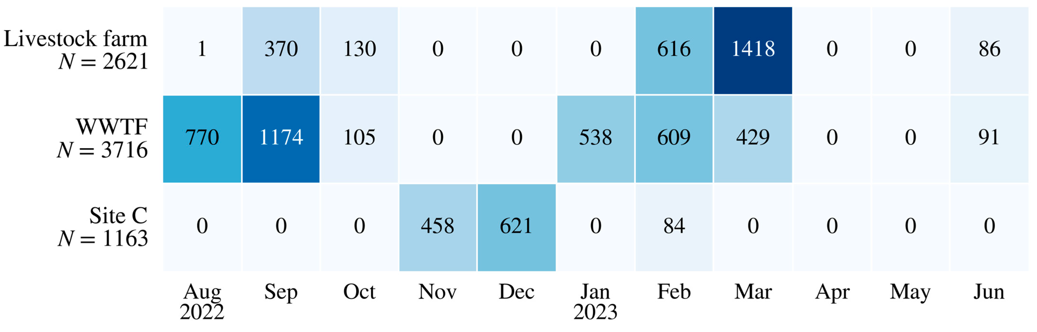
The number of simultaneous H2S and NH3 observations was 2621 at the livestock farm, 3716 at the wastewater treatment facility, and 1163 at Site C, yielding a total of 7500 observations. The final analysis datasets, in which the target compound and all required covariates were observed, contained 5442–6333 observations per target in the development dataset and 974–1163 observations per target at Site C. The development dataset contained 24–25 site–week groups depending on the target, whereas Site C consisted of four calendar-week groups for all targets.
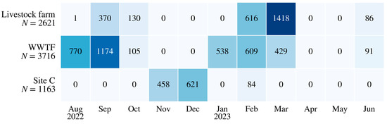
The monthly distribution of simultaneous H2S and NH3 observations differed among sites. At Site C, 458 simultaneous observations were available in November 2022, 621 in December 2022, and 84 in February 2023. February 2023 was the only observation month shared between the development sites and the external site. Accordingly, the Site C evaluation provided an independent validation setting in which the models were applied under different site and observation-period conditions from those of the development dataset [34].
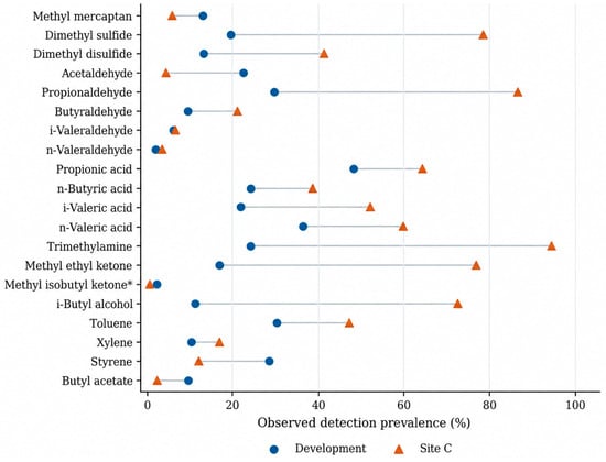
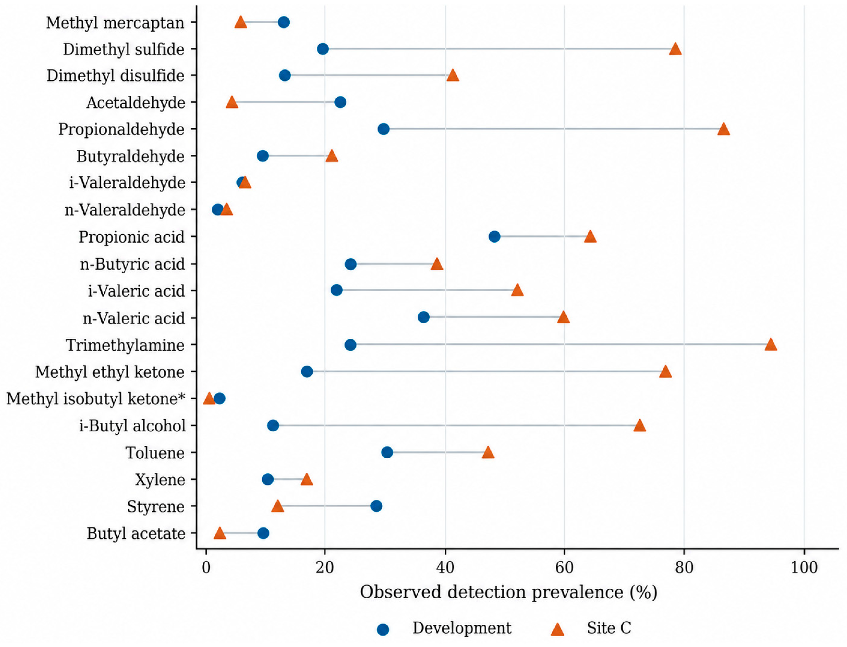
Detection prevalence was higher at Site C than in the development dataset for 15 of the 20 targets. In the development dataset, prevalence ranged from 1.58% for methyl isobutyl ketone to 48.25% for propionic acid, whereas at Site C it ranged from 0.10% to 94.97%. The prevalence of dimethyl sulfide increased from 19.31% in the development dataset to 78.54% at Site C, and that of trimethylamine increased from 24.09% to 94.97%, whereas methyl mercaptan decreased from 12.98% to 5.76%. Whereas Figure 2 illustrates the imbalance in observation periods, Figure 3 shows that the class composition of the same targets differed between the development and external evaluation domains. This difference provides important context for interpreting absolute AP values and alarm burden [28,43].
Figure 2.
Monthly simultaneous observations of H2S and NH3.
Figure 3.
Detection prevalence of the 20 target compounds. Detection was defined as a concentration at or above the compound-specific detection limit. An asterisk identifies methyl isobutyl ketone as an exploratory target.
3.2. Selection of Compound-Specific Alarm Models and Probability Calibration
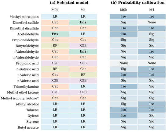
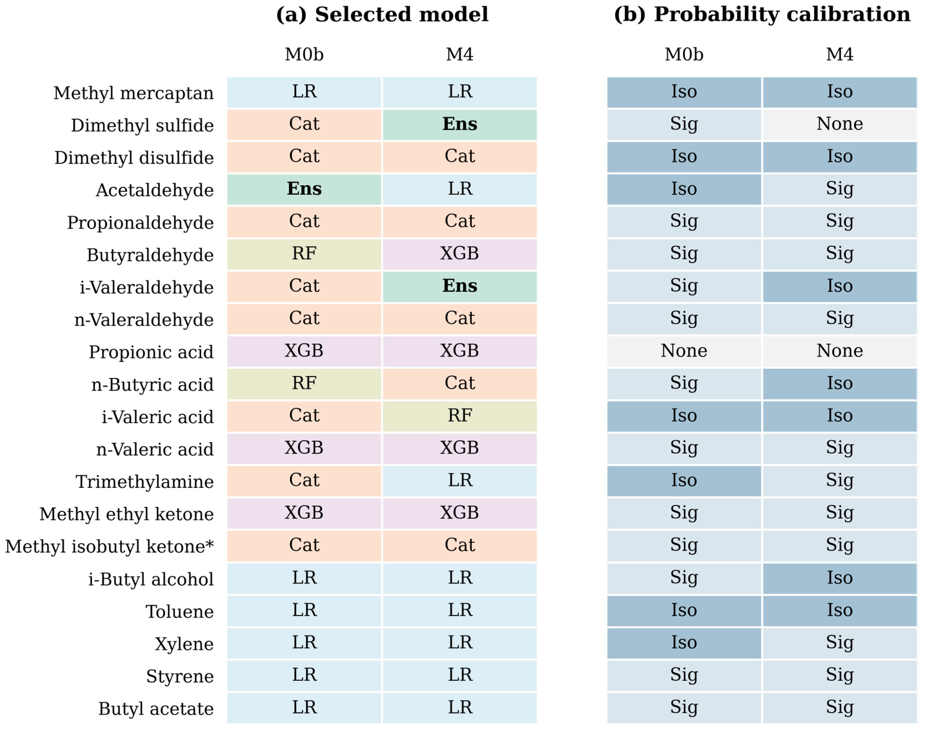
The final selected models and probability-calibration methods are shown in Figure 4, and the frequencies of model selection by input-variable set are summarized in Table 2. CatBoost was selected most frequently for M0b, being chosen for eight targets, whereas logistic regression was selected most frequently for M4, also for eight targets. The equal-weight soft-voting ensemble (Ens) was selected for three of the 40 target–input-set combinations: M0b for acetaldehyde and M4 for dimethyl sulfide and i-valeraldehyde. The selected probability-calibration methods consisted of sigmoid calibration for 23 combinations, isotonic calibration for 14 combinations, and no calibration for three combinations.
Figure 4.
Selected models and calibration methods. * Methyl isobutyl ketone was treated as an exploratory target.
Table 2.
Distribution of the final models selected using the full development dataset.
The variation in selected models and calibration methods among targets indicates that no single algorithm was equally suitable for all odor compounds. The selection of logistic regression for eight M4 targets suggests that relatively simple relationships on the log-odds scale were sufficient to achieve competitive performance for some compounds within the evaluated candidate set. Tree-based models selected for other targets can accommodate nonlinear relationships and interactions among chemical and meteorological inputs. These differences may reflect variation in detection prevalence, co-emission patterns, and environmental conditions, but may also arise from sample availability and the limited hyperparameter search. Because model selection was not systematically analyzed by chemical class or emission dynamics, the selected algorithms should not be interpreted as direct evidence of compound-specific chemical mechanisms. Accordingly, the present study focused on the performance difference between the M0b and M4 alarm pipelines under the same candidate-selection procedure rather than on the superiority of any individual algorithm.
3.3. Detection Classification Performance in the Development Dataset
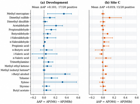
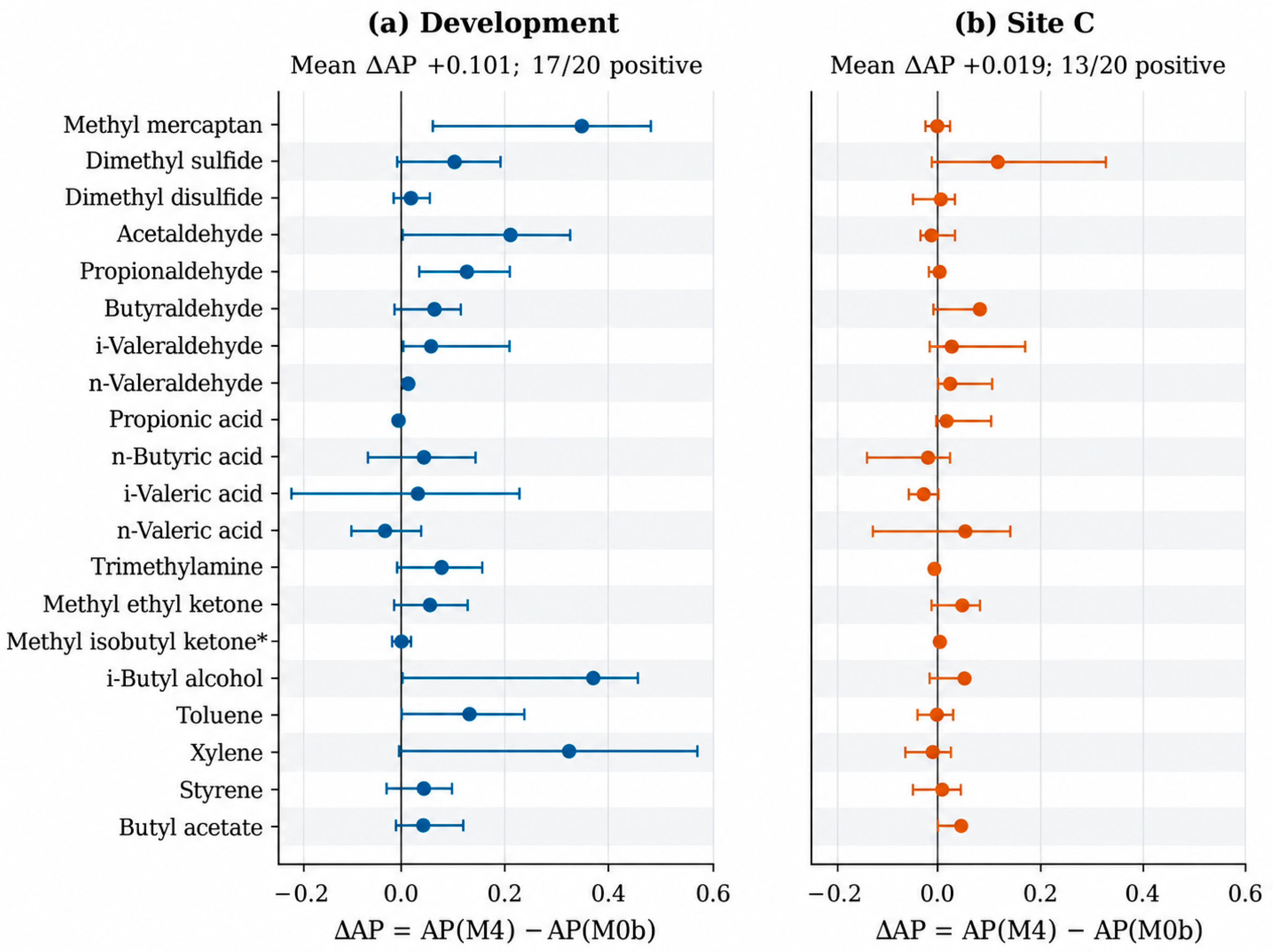
In the development dataset, the mean AP across the 20 targets increased from 0.362 for M0b to 0.463 for M4, corresponding to a mean ΔAP of +0.101. AP increased for 17 targets, with the largest increases observed for i-butyl alcohol (+0.374), methyl mercaptan (+0.351), xylene (+0.333), and acetaldehyde (+0.208) (Figure 5a). When the exploratory target methyl isobutyl ketone was excluded, the mean ΔAP across the remaining 19 targets was approximately +0.106, showing the same overall direction as the 20-target mean.
Figure 5.
ΔAP for the development and external datasets. * Methyl isobutyl ketone was treated as an exploratory target.
The lower bound of the cluster-bootstrap 95% confidence interval for ΔAP was greater than zero for four targets: methyl mercaptan, acetaldehyde, propionaldehyde, and i-valeraldehyde. Although i-butyl alcohol showed the largest increase, with a ΔAP of +0.374, the lower confidence-limit bound was −0.00050. The minimum BH-adjusted q-value was 0.0798 and therefore did not reach the predefined criterion of q < 0.05; nevertheless, a consistent signal of improved performance after adding H2S and NH3 was observed across multiple targets. Target-specific AP values, ΔAP values, confidence intervals, and q-values are provided in Table A3.
The increase in AP for 17 of the 20 targets and the mean ΔAP of +0.101 indicate that H2S and NH3 can provide additional classification information beyond the meteorological and temporal information included in the baseline model. These findings suggest the potential for using a limited number of chemical signals to simultaneously screen the detection status of multiple odorants. However, because the magnitude of improvement differed among compounds, target-specific response characteristics were further examined in the external evaluation.
3.4. Detection Classification Performance at the Independent Site
At Site C, the mean AP across the 20 targets increased from 0.424 for M0b to 0.443 for M4, corresponding to a mean ΔAP of +0.019. AP increased for 13 targets (Figure 5b). Dimethyl sulfide showed the largest increase, with a ΔAP of +0.116 and an M4 AP of 0.873. Positive ΔAP values were also observed for butyraldehyde (+0.076), n-valeric acid (+0.053), i-butyl alcohol (+0.051), methyl ethyl ketone (+0.048), and butyl acetate (+0.042). These findings indicate that the additional information provided by H2S and NH3 was retained for several targets even at a new facility.
The lower confidence-limit bound was greater than zero for n-valeraldehyde and the exploratory target methyl isobutyl ketone. Because Site C consisted of four calendar weeks, the exact week-level permutation test had only 16 possible exchange combinations, resulting in a minimum attainable two-sided p-value of 0.125. Thus, the statistical resolution of the external evaluation was structurally limited. Accordingly, the BH-adjusted results were interpreted together with effect sizes and target-specific trends. Methyl isobutyl ketone was retained as an exploratory target because the development dataset contained only 86 positive observations; its external evaluation was further limited by only one positive observation at Site C. After excluding this target, the mean ΔAP across the remaining 19 targets remained positive at +0.020.
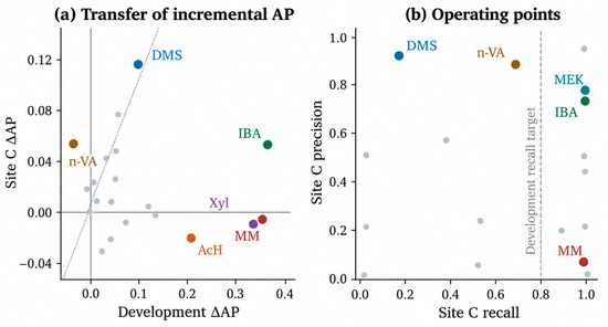
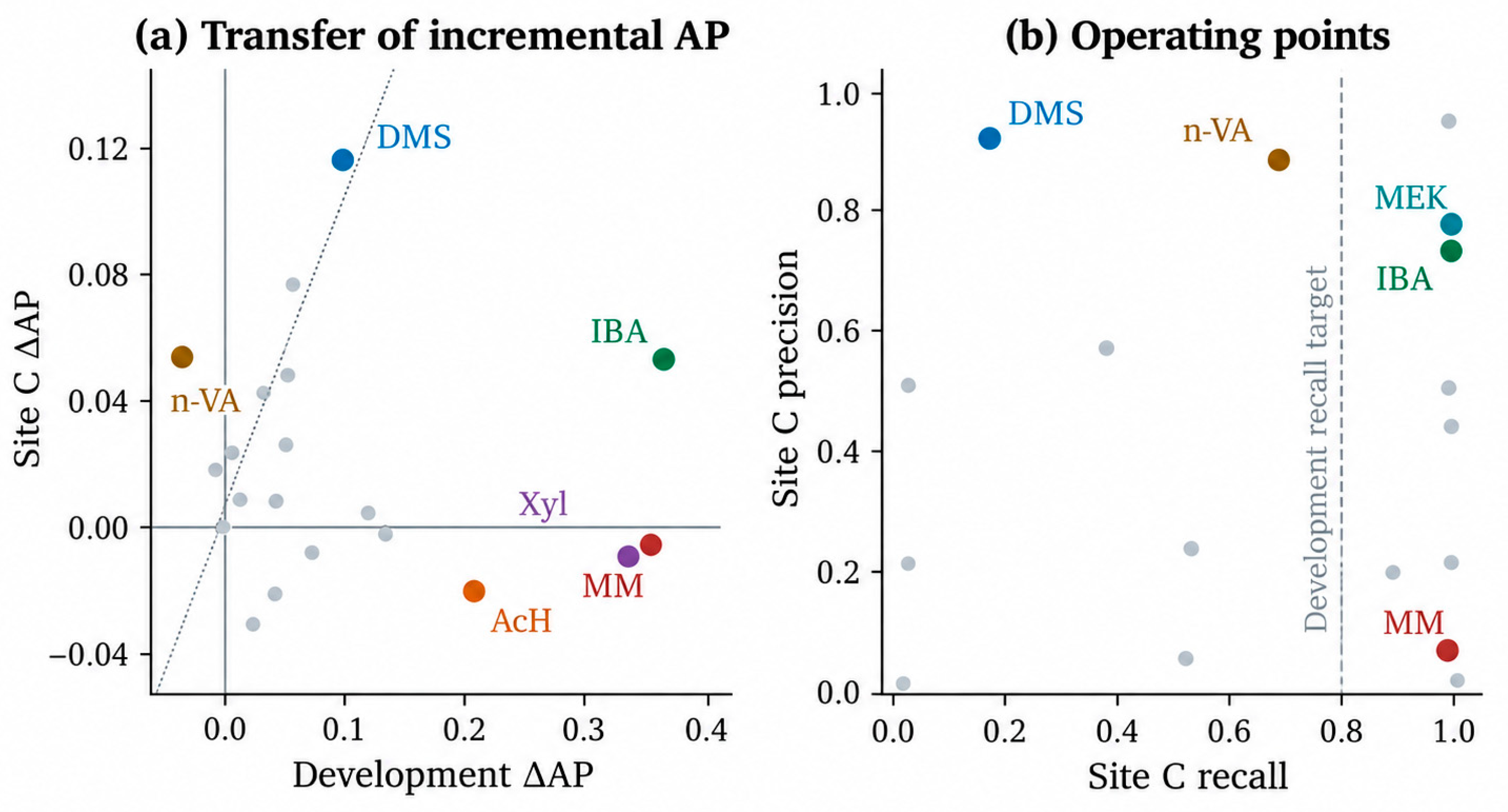
Of the 17 targets for which AP increased in the development dataset, 10 also retained a positive ΔAP at Site C. In particular, dimethyl sulfide showed similar positive improvements in both evaluation domains, with ΔAP values of +0.104 in the development dataset and +0.116 at Site C. For several targets, including methyl mercaptan, xylene, and acetaldehyde, the magnitude or direction of external ΔAP differed from that observed during development, indicating that the classification information provided by H2S and NH3 may vary according to both the target compound and facility conditions [34,44]. Therefore, the external results were interpreted primarily in terms of compound-specific response characteristics rather than a single overall mean value. The detection prevalence, M4 AP, and ΔAP for all 20 targets at Site C are summarized in Table 3.
Table 3.
External performance of the M4 detection-alarm models at Site C.
Site C also showed positive ΔAP values for 13 targets, suggesting that H2S and NH3 may provide additional classification information for some targets under external conditions. Dimethyl sulfide, in particular, showed a positive ΔAP in both the development dataset and Site C, indicating a relatively consistent direction of improvement. Differences in the magnitude of improvement among compounds suggest that the information value of the two gases may depend on facility-specific emission characteristics and target-specific detection prevalence [43,44].
The prevalence shifts also affect the interpretation of absolute AP values [43]. For trimethylamine, prevalence increased from 24.09% in development to 94.97% at Site C; although the external M4 AP was 0.977, ΔAP was −0.008. Thus, a high external AP did not necessarily indicate an improvement from adding H2S and NH3. For i-butyl alcohol, prevalence increased from 11.06% to 72.69%, while ΔAP decreased from +0.374 in development to +0.051 externally. Its external M4 alarm rate and recall were both 1.000, with precision equal to prevalence (0.727), indicating that all observations were classified as positive. These examples show why AP should be interpreted alongside prevalence and fixed-threshold metrics. Changes in prevalence and other aspects of the data distribution may compromise probability calibration and threshold transfer [44]. However, the present analysis does not isolate the contribution of prevalence shifts from changes in predictor distributions or predictor–outcome relationships.
The availability of only four calendar-week groups substantially limits the strength of the external evidence. Although many observations were collected within these weeks, repeated observations do not compensate for the small number of independent evaluation units. Accordingly, the observed ΔAP values describe compound-specific performance changes but do not provide confirmatory evidence of generalizability.
For the two-sided exchange test used here, the minimum attainable p-value with G independent groups is 2/2G. Thus, at least six groups are required for an unadjusted p-value below 0.05 to be theoretically attainable. This is a requirement for p-value resolution, not a sufficient sample size for adequate statistical power or significance after multiple-comparison correction. The required number of independent site–week groups depends on the target effect size, between-group variability, detection prevalence, temporal dependence, and multiplicity adjustment. The four external groups available here are insufficient to estimate these characteristics reliably for sample-size planning. Future validation should therefore include additional facilities and observation periods, with simulation-based sample-size planning reflecting the grouped design and multiple-testing procedure.
3.5. Fixed-Threshold Detection-Alarm Performance at the Independent Site
The compound-specific models, probability-calibration functions, and decision thresholds determined from the development dataset were applied to Site C without modification to evaluate actual alarm performance. Interpretation focused on M4 precision, recall, false-positive rate, FAP, alarm rate, and event recall, with M0b used as the reference. Detailed operating metrics for six representative targets are provided in Table A4.
For dimethyl sulfide, M4 precision increased from 0.775 for M0b to 0.921, while the false-positive rate decreased markedly from 0.464 to 0.057. At the same time, the proportion of all observations classified as alarms decreased from 0.443 to 0.155, indicating a more selective alarm pattern, whereas recall decreased from 0.437 to 0.182. For n-valeric acid, precision increased from 0.656 to 0.882, the alarm rate decreased from 0.877 to 0.462, and recall was 0.681. These results indicate that M4, which incorporated H2S and NH3, could increase alarm selectivity at the external facility while also highlighting the need to balance recall and precision according to the intended operational objective [28,31].
For dimethyl sulfide, the recall of 0.182 means that 81.8% of positive observations were missed under the transferred threshold. Such an operating point may be considered for prioritizing a limited number of confirmatory analyses only when routine monitoring continues independently and the absence of an alarm is not interpreted as evidence of non-detection. It is unsuitable as the sole screening trigger when high detection coverage is required. Where missed detections are operationally unacceptable, the threshold should be reselected using a separate, representative site-specific calibration dataset to meet a predefined recall requirement, with the resulting precision and alarm burden assessed explicitly. The adjusted operating point should then be evaluated on independent data. The present Site C results retain the original development thresholds and do not demonstrate the performance achievable after such adjustment. Sensitivity to alternative development recall requirements was not evaluated; therefore, the extent to which the reported external operating metrics depend on the choice of 0.80 remains uncertain. Future evaluation should compare alternative requirements using thresholds selected exclusively from development data and assess their effects on external recall, precision, and alarm rate.
For methyl ethyl ketone, both M0b and M4 classified all Site C observations as alarms, and high alarm sensitivity was also observed for M4 in i-butyl alcohol and n-valeraldehyde. In particular, recall for methyl mercaptan increased markedly from 0.552 for M0b to 0.985 for M4. The M4 alarm rate for methyl mercaptan was also high at 0.986, indicating that a sensitivity-oriented operating point was selected for this compound. These examples show that M4 may produce either selectivity-oriented or sensitivity-oriented alarm characteristics depending on the target and that, in practical applications, the threshold may be adjusted according to the intended operational objective [31].
The external application results showed that changes in AP after adding H2S and NH3 and performance at fixed decision thresholds provided complementary information [28,30,31]. For dimethyl sulfide and n-valeric acid, selectivity improved in terms of precision and false-positive rate, whereas some compounds, such as methyl mercaptan, exhibited sensitivity-oriented alarm characteristics with high recall.
The fixed-threshold evaluation also showed that operating characteristics differed among targets, with some favoring selectivity and others sensitivity. Dimethyl sulfide and n-valeric acid showed increased precision and reduced false-positive rates, whereas methyl mercaptan exhibited high recall. These results indicate that target-specific thresholds tailored to the intended objective are more appropriate for practical alarm operation than a single common operating criterion [31].
3.6. Relationship Between Classification Performance and Alarm Operating Points
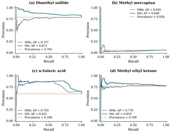
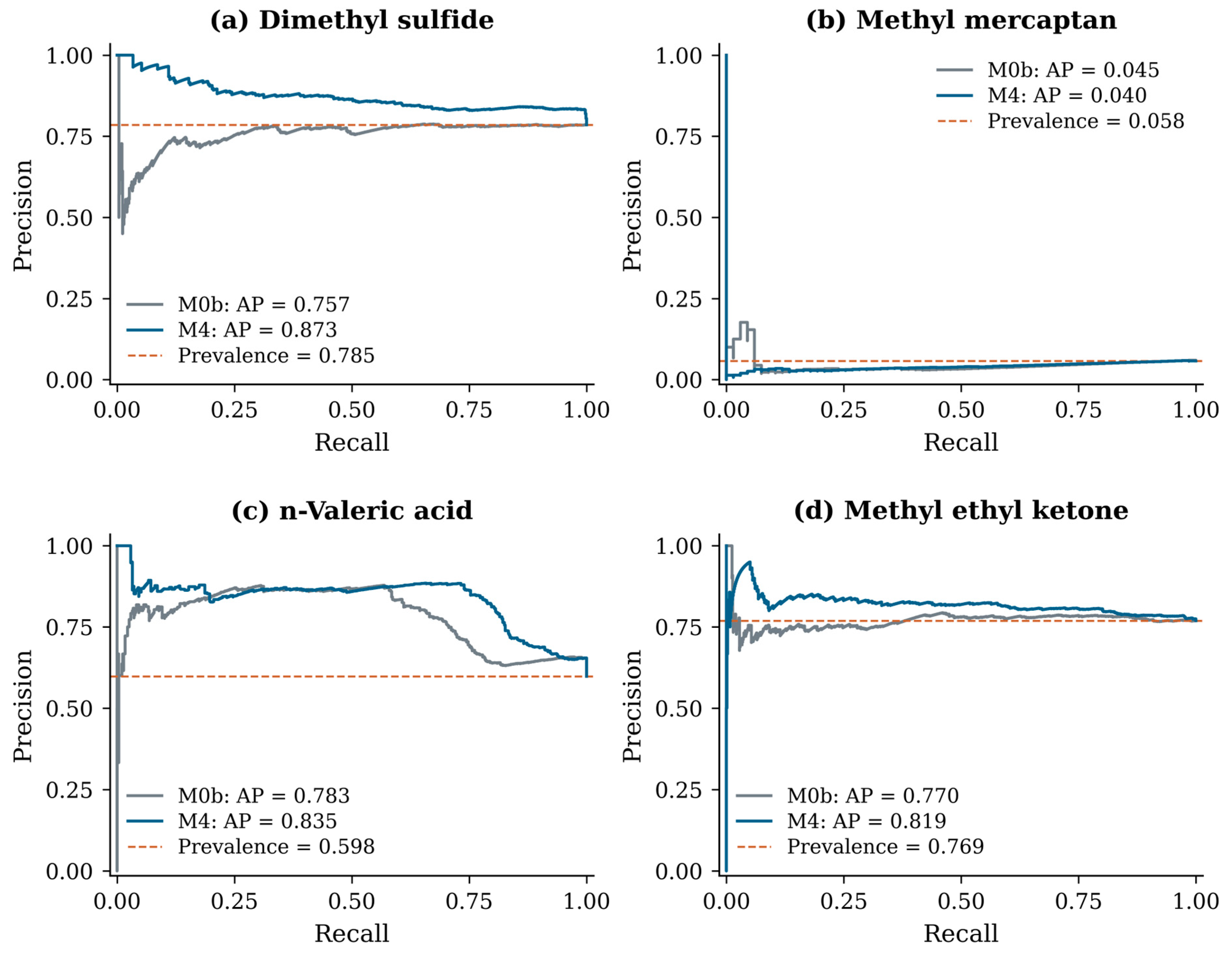
Operating points obtained by applying the fixed thresholds to the calibrated probabilities are presented separately in Figure 6b and Table A4. Figure 7 presents four illustrative targets selected to contrast improvements in ranking performance with different fixed-threshold alarm patterns, including selective alarms and near-continuous alarms. These examples were chosen to illustrate operational differences rather than to represent performance across all 20 targets. The M4 AP values for dimethyl sulfide and n-valeric acid were 0.873 and 0.835, respectively, indicating relatively high classification performance, while the M4 AP for methyl ethyl ketone was also higher than that of M0b at 0.819. However, different target-specific operating points were obtained under the fixed thresholds. This demonstrates that the ranking-based AP metric and the actual alarm operating point provide different information and that, at an external facility, probability calibration and threshold adjustment are important for translating classification performance into the desired alarm characteristics [28,30,31].
Figure 6.
External transfer and operating characteristics of the detection-alarm models. Dotted line: equal ΔAP (a); dashed line: development recall target of 0.80 (b); gray dots: other compounds.
Figure 7.
Representative precision–recall curves of four target compounds at Site C.
The precision–recall curves were generated using uncalibrated probabilities. Because isotonic calibration can produce tied probability values, the operating points based on calibrated probabilities were not superimposed on the uncalibrated precision–recall curves [30].
In practical use, an operator could use compound-specific alarms to prioritize target compounds and sampling times for confirmatory chemical analysis, alongside routine monitoring and site operating records. The minimum measurement configuration for the current M4 model comprises H2S, NH3, air temperature, relative humidity, wind speed, and wind direction, together with synchronized timestamps for deriving the cyclical time variables. All required inputs must be available and aligned at the same observation time. Before deployment, the intended instruments should be checked for measurement compatibility with the development data, and the model and thresholds should undergo site-specific validation. An alarm indicates a model-estimated analytical detection state, rather than a measured concentration or regulatory exceedance, and the absence of an alarm should not be used to suspend routine monitoring.
Because Site C consisted of only four calendar weeks, the statistical resolution of the external evaluation was limited. Therefore, external performance was interpreted by considering not only statistical significance but also the direction and magnitude of ΔAP and the fixed-threshold operating metrics. In addition, the alarms evaluated in this study represent analytical detection status at the same observation time and are distinct from early-warning systems intended to predict sensory odor intensity or future odor occurrence.
4. Conclusions
This study developed machine-learning-based detection-alarm algorithms for individually determining the analytical detection status of the remaining 20 odorants using H2S and NH3 as the core chemical inputs and meteorological and temporal information as supplementary inputs. Compound-specific detection probability estimation, probability calibration, and alarm-threshold selection were integrated into a single analytical procedure, and the models finalized using data from the livestock farm and wastewater treatment facility were applied to the independent Site C without modification. In internal cross-validation, the mean AP increased from 0.362 to 0.463, and AP improved for 17 of the 20 target compounds after the addition of H2S and NH3. At Site C, the mean AP also increased from 0.424 to 0.443, with positive ΔAP values observed for 13 compounds, demonstrating the potential of using a limited number of chemical signals for multi-compound detection classification. However, the external evaluation was restricted to four calendar-week groups, and no compound-specific improvement reached BH-adjusted statistical significance. These external results should therefore be interpreted as exploratory, with broader generalizability requiring validation across additional facilities and observation periods.
Under fixed-threshold operation, the models exhibited different advantages depending on the target compound. For dimethyl sulfide, M4 achieved a precision of 0.921 and a false-positive rate of 0.057, but the recall was 0.182. Methyl mercaptan achieved a recall of 0.985, accompanied by an alarm rate of 0.986 and a precision of 0.058, illustrating the trade-off between detection coverage and alarm burden. These findings demonstrate the importance of setting compound-specific thresholds according to the intended operational objective rather than applying a single common operating criterion. They also suggest that practical alarm characteristics can be designed by jointly considering AP, precision, recall, false-positive rate, and alarm frequency.
The H2S- and NH3-based multi-compound odor detection-alarm framework provides a practical approach for simultaneously assessing the detectability of multiple target compounds using a small number of core chemical signals and translating these assessments into compound-specific alarms. In particular, the increase in AP for 17 of 20 targets in the internal evaluation and for 13 targets in the independent external evaluation indicates that H2S and NH3 may serve as useful supplementary signals for multi-component odor monitoring. The compound-specific differences in operating points observed at the external facility further indicate that alarm performance may be optimized through site-specific threshold adjustment and sensor-based validation. The current models should not be deployed without additional validation at facilities with substantially different emission profiles or for targets with insufficient positive observations. The fixed-threshold alarms are also unsuitable as the sole basis for decisions requiring high detection coverage, and the absence of an alarm should not be interpreted as confirmation that a target compound is absent. Therefore, rather than replacing costly multi-component chemical analyses, the proposed framework may serve as a basis for a data-driven supplementary alarm system that uses a limited number of continuously measured signals to prioritize compounds requiring additional analysis or field response.
Author Contributions
Conceptualization, C.-H.K. and D.-C.S.; methodology, C.-H.K.; software, C.-H.K.; validation, C.-H.K. and D.-C.S.; formal analysis, C.-H.K.; investigation, C.-H.K.; resources, D.-C.S.; data curation, C.-H.K.; writing—original draft preparation, C.-H.K.; writing—review and editing, D.-C.S.; visualization, C.-H.K.; supervision, D.-C.S.; project administration, D.-C.S.; funding acquisition, D.-C.S. All authors have read and agreed to the published version of the manuscript.
Funding
This research received no external funding.
Institutional Review Board Statement
Not applicable.
Informed Consent Statement
Not applicable.
Data Availability Statement
The data presented in this study are not publicly available because they were obtained from a private company and are subject to confidentiality and data-use restrictions.
Acknowledgments
This work was supported by the Daejin University Research Grants in 2026.
Conflicts of Interest
The authors declare no conflicts of interest. The funders had no role in the design of the study; in the collection, analysis, or interpretation of data; in the writing of the manuscript; or in the decision to publish the results.
Abbreviations
The following abbreviations are used in this manuscript:
| AP | Average precision |
| BH | Benjamini–Hochberg false-discovery-rate correction |
| DL | Detection limit |
| FAP | False-alarm proportion |
| FPR | False-positive rate |
| H2S | Hydrogen sulfide |
| NH3 | Ammonia |
| LR | Logistic regression |
| M0b | Meteorological–temporal baseline model |
| M4 | M0b + H2S + NH3 |
| OOF | Out-of-fold |
| RF | Random forest |
| TD-GC-FID | Thermal-desorption gas chromatography with flame-ionization detection |
| TD-GC-PID | Thermal-desorption gas chromatography with photoionization detection |
| TDLS | Tunable diode laser spectroscopy |
| WWTF | Wastewater treatment facility |
Appendix A
Table A1.
Detection limits and dataset composition for the 20 target compounds.
Table A2.
Hyperparameter search spaces for candidate models and fixed settings of ensemble components.
Table A3.
Target-specific AP, paired ΔAP, cluster-bootstrap 95% confidence intervals, and BH-adjusted q-values.
Table A4.
Fixed-threshold operating metrics for six representative target compounds at Site C.
References
- Dentoni, L.; Capelli, L.; Sironi, S.; Del Rosso, R.; Zanetti, S.; Della Torre, M. Development of an Electronic Nose for Environmental Odour Monitoring. Sensors 2012, 12, 14363–14381. [Google Scholar] [CrossRef] [Scilit]
- Capelli, L.; Sironi, S.; Del Rosso, R. Electronic Noses for Environmental Monitoring Applications. Sensors 2014, 14, 19979–20007. [Google Scholar] [CrossRef] [Scilit]
- Cipriano, D.; Capelli, L. Evolution of Electronic Noses from Research Objects to Engineered Environmental Odour Monitoring Systems: A Review of Standardization Approaches. Biosensors 2019, 9, 75. [Google Scholar] [CrossRef] [Scilit]
- Sironi, S.; Capelli, L.; Céntola, P.; Del Rosso, R.; Il Grande, M. Continuous Monitoring of Odours from a Composting Plant Using Electronic Noses. Waste Manag. 2007, 27, 389–397. [Google Scholar] [CrossRef] [Scilit]
- Capelli, L.; Sironi, S.; Del Rosso, R.; Céntola, P. Predicting Odour Emissions from Wastewater Treatment Plants by Means of Odour Emission Factors. Water Res. 2009, 43, 1977–1985. [Google Scholar] [CrossRef] [Scilit]
- Blanco-Rodríguez, A.; Camara, V.F.; Campo, F.; Becherán, L.; Durán, A.; Vieira, V.D.; de Melo, H.; Garcia-Ramirez, A.R. Development of an Electronic Nose to Characterize Odours Emitted from Different Stages in a Wastewater Treatment Plant. Water Res. 2018, 134, 92–100. [Google Scholar] [CrossRef] [Scilit]
- Burgués, J.; Esclapez, M.D.; Doñate, S.; Marco, S. RHINOS: A Lightweight Portable Electronic Nose for Real-Time Odor Quantification in Wastewater Treatment Plants. iScience 2021, 24, 103371. [Google Scholar] [CrossRef] [Scilit]
- Wang, B.; Li, X.; Chen, D.; Weng, X.; Chang, Z. Development of an Electronic Nose to Characterize Water Quality Parameters and Odor Concentration of Wastewater Emitted from Different Phases in a Wastewater Treatment Plant. Water Res. 2023, 235, 119878. [Google Scholar] [CrossRef] [Scilit]
- Zarra, T.; Galang, M.G.K.; Oliva, G.; Belgiorno, V. Smart Instrumental Odour Monitoring Station for the Efficient Odour Emission Management and Control in Wastewater Treatment Plants. Chemosphere 2022, 309, 136665. [Google Scholar] [CrossRef] [Scilit]
- Prudenza, S.; Panzitta, A.; Bax, C.; Capelli, L. Electronic Nose for Real-Time Monitoring of Odour Emissions at a Wastewater Treatment Plant. Chem. Eng. Trans. 2022, 95, 169–174. [Google Scholar] [CrossRef]
- Prudenza, S.; Bax, C.; Capelli, L. Implementation of an Electronic Nose for Real-Time Identification of Odour Emission Peaks at a Wastewater Treatment Plant. Heliyon 2023, 9, e20437. [Google Scholar] [CrossRef] [Scilit]
- Ratti, C.; Bax, C.; Lotesoriere, B.J.; Capelli, L. Real-Time Monitoring of Odour Emissions at the Fenceline of a Waste Treatment Plant by Instrumental Odour Monitoring Systems: Focus on Training Methods. Sensors 2024, 24, 3506. [Google Scholar] [CrossRef] [Scilit]
- Wang, B.; Yan, Y.; An, R.; Weng, X.; Chang, Z. Application of Electronic Nose Technology in Wastewater Treatment Plants Monitoring: Progress and Future Developments. Microchem. J. 2026, 224, 117768. [Google Scholar] [CrossRef] [Scilit]
- Talaiekhozani, A.; Bagheri, M.; Goli, A.; Talaei Khoozani, M.R. An Overview of Principles of Odor Production, Emission, and Control Methods in Wastewater Collection and Treatment Systems. J. Environ. Manag. 2016, 170, 186–206. [Google Scholar] [CrossRef] [Scilit]
- Jiang, G.; Melder, D.; Keller, J.; Yuan, Z. Odor Emissions from Domestic Wastewater: A Review. Crit. Rev. Environ. Sci. Technol. 2017, 47, 1581–1611. [Google Scholar] [CrossRef] [Scilit]
- Senatore, V.; Zarra, T.; Galang, M.G.; Oliva, G.; Buonerba, A.; Li, C.-W.; Belgiorno, V.; Naddeo, V. Full-Scale Odor Abatement Technologies in Wastewater Treatment Plants (WWTPs): A Review. Water 2021, 13, 3503. [Google Scholar] [CrossRef] [Scilit]
- González, D.; Gabriel, D.; Sánchez, A. Odors Emitted from Biological Waste and Wastewater Treatment Plants: A Mini-Review. Atmosphere 2022, 13, 798. [Google Scholar] [CrossRef] [Scilit]
- Toledo, M.; Muñoz, R. Odour Prevention Strategies in Wastewater Treatment and Composting Plants: A Review. J. Environ. Manag. 2025, 375, 124402. [Google Scholar] [CrossRef] [Scilit]
- Wang, Y.-C.; Han, M.-F.; Jia, T.-P.; Hu, X.-R.; Zhu, H.-Q.; Tong, Z.; Lin, Y.-T.; Wang, C.; Liu, D.-Z.; Peng, Y.-Z.; et al. Emissions, Measurement, and Control of Odor in Livestock Farms: A Review. Sci. Total Environ. 2021, 776, 145735. [Google Scholar] [CrossRef] [Scilit]
- Cao, T.; Zheng, Y.; Dong, H. Control of Odor Emissions from Livestock Farms: A Review. Environ. Res. 2023, 225, 115545. [Google Scholar] [CrossRef] [Scilit]
- Lee, S.-H.; Bae, S. A Strategy for Ammonia Odor Monitoring, Prediction, and Reduction from Livestock Manure Wastes in Korea: A Short Review. Geosyst. Eng. 2022, 25, 35–43. [Google Scholar] [CrossRef] [Scilit]
- Joo, H.; Han, S.-W.; Lee, C.-S.; Jang, H.-S.; Kim, S.-T.; Han, J.-S. Field Application of Cost-Effective Sensors for the Monitoring of NH3, H2S, and TVOC in Environmental Treatment Facilities and the Estimation of Odor Intensity. J. Air Waste Manag. Assoc. 2023, 73, 50–64. [Google Scholar] [CrossRef] [Scilit]
- Kim, J.H.; Rene, E.R.; Park, S.H.; Park, H.S. Effect of Inlet Loading Rate on the Elimination of Hydrogen Sulfide and Ammonia in Immobilized Cell Biofilters. Environ. Eng. Res. 2006, 11, 285–291. [Google Scholar] [CrossRef] [Scilit]
- Ren, Y.; Zhang, R.; Zhang, L.; Wang, H.; Zhang, X.; Bai, Z.; Ma, L.; Wang, X. The Characteristics of Key Odorants from Livestock Farms and Their Mitigation Potential: A Meta-Analysis. Atmosphere 2025, 16, 1097. [Google Scholar] [CrossRef] [Scilit]
- Sinharoy, A.; Kim, S.H.; Chung, C.M. Effect of Variation in Temperature on Malodor Generation from Different Units of a Wastewater Treatment Plant. Environ. Sci. Pollut. Res. 2025, 32, 8035–8052. [Google Scholar] [CrossRef] [Scilit]
- He, H.; Garcia, E.A. Learning from Imbalanced Data. IEEE Trans. Knowl. Data Eng. 2009, 21, 1263–1284. [Google Scholar] [CrossRef] [Scilit]
- Davis, J.; Goadrich, M. The Relationship between Precision-Recall and ROC Curves. In Proceedings of the 23rd International Conference on Machine Learning, Pittsburgh, PA, USA, 25–29 June 2006; pp. 233–240. [Google Scholar] [CrossRef] [Scilit]
- Saito, T.; Rehmsmeier, M. The Precision-Recall Plot Is More Informative than the ROC Plot When Evaluating Binary Classifiers on Imbalanced Datasets. PLoS ONE 2015, 10, e0118432. [Google Scholar] [CrossRef] [Scilit]
- Fawcett, T. An Introduction to ROC Analysis. Pattern Recognit. Lett. 2006, 27, 861–874. [Google Scholar] [CrossRef] [Scilit]
- Niculescu-Mizil, A.; Caruana, R. Predicting Good Probabilities with Supervised Learning. In Proceedings of the 22nd International Conference on Machine Learning, Bonn, Germany, 7–11 August 2005; pp. 625–632. [Google Scholar] [CrossRef] [Scilit]
- Collell, G.; Prelec, D.; Patil, K.R. A Simple Plug-In Bagging Ensemble Based on Threshold-Moving for Classifying Binary and Multiclass Imbalanced Data. Neurocomputing 2018, 275, 330–340. [Google Scholar] [CrossRef] [Scilit]
- Roberts, D.R.; Bahn, V.; Ciuti, S.; Boyce, M.S.; Elith, J.; Guillera-Arroita, G.; Hauenstein, S.; Lahoz-Monfort, J.J.; Schröder, B.; Thuiller, W.; et al. Cross-Validation Strategies for Data with Temporal, Spatial, Hierarchical, or Phylogenetic Structure. Ecography 2017, 40, 913–929. [Google Scholar] [CrossRef] [Scilit]
- Valavi, R.; Elith, J.; Lahoz-Monfort, J.J.; Guillera-Arroita, G. blockCV: An R Package for Generating Spatially or Environmentally Separated Folds for k-Fold Cross-Validation of Species Distribution Models. Methods Ecol. Evol. 2019, 10, 225–232. [Google Scholar] [CrossRef] [Scilit]
- Ho, S.Y.; Phua, K.; Wong, L.; Goh, W.W.B. Extensions of the External Validation for Checking Learned Model Interpretability and Generalizability. Patterns 2020, 1, 100129. [Google Scholar] [CrossRef] [Scilit]
- Kim, C.-h.; Shin, D.-c.; Kim, M.-w. OAV-Based Source Characterization of Designated Odor Compounds in Long-Term Continuous Monitoring Data with Severe Missingness. Atmosphere 2026, 17, 868. [Google Scholar] [CrossRef] [Scilit]
- Breiman, L. Random Forests. Mach. Learn. 2001, 45, 5–32. [Google Scholar] [CrossRef] [Scilit]
- Chen, T.; Guestrin, C. XGBoost: A Scalable Tree Boosting System. In Proceedings of the 22nd ACM SIGKDD International Conference on Knowledge Discovery and Data Mining, San Francisco, CA, USA, 13–17 August 2016; pp. 785–794. [Google Scholar] [CrossRef] [Scilit]
- Prokhorenkova, L.; Gusev, G.; Vorobev, A.; Dorogush, A.V.; Gulin, A. CatBoost: Unbiased Boosting with Categorical Features. Adv. Neural Inf. Process. Syst. 2018, 31, 6638–6648. [Google Scholar]
- Kittler, J.; Hatef, M.; Duin, R.P.W.; Matas, J. On Combining Classifiers. IEEE Trans. Pattern Anal. Mach. Intell. 1998, 20, 226–239. [Google Scholar] [CrossRef] [Scilit]
- Varma, S.; Simon, R. Bias in Error Estimation When Using Cross-Validation for Model Selection. BMC Bioinform. 2006, 7, 91. [Google Scholar] [CrossRef] [Scilit]
- Brier, G.W. Verification of Forecasts Expressed in Terms of Probability. Mon. Weather Rev. 1950, 78, 1–3. [Google Scholar] [CrossRef] [Scilit]
- Benjamini, Y.; Hochberg, Y. Controlling the False Discovery Rate: A Practical and Powerful Approach to Multiple Testing. J. R. Stat. Soc. Ser. B 1995, 57, 289–300. [Google Scholar] [CrossRef] [Scilit]
- Williams, C.K.I. The Effect of Class Imbalance on Precision-Recall Curves. Neural Comput. 2021, 33, 853–857. [Google Scholar] [CrossRef] [Scilit]
- Dockès, J.; Varoquaux, G.; Poline, J.-B. Preventing Dataset Shift from Breaking Machine-Learning Biomarkers. GigaScience 2021, 10, giab055. [Google Scholar] [CrossRef] [Scilit]

Disclaimer/Publisher’s Note: The statements, opinions and data contained in all publications are solely those of the individual author(s) and contributor(s) and not of MDPI and/or the editor(s). MDPI and/or the editor(s) disclaim responsibility for any injury to people or property resulting from any ideas, methods, instructions or products referred to in the content. |
© 2026 by the authors. Licensee MDPI, Basel, Switzerland. This article is an open access article distributed under the terms and conditions of the Creative Commons Attribution (CC BY) license.