


Abstract
Airborne pollen is a major public health concern due to its allergenic properties. Understanding long-term changes in pollen dynamics is essential for evaluating shifts in exposure to airborne allergens and enhancing allergy risk management. In this study we examine long-term trends in airborne pollen in the urban area of Bolzano, the capital city of the Autonomous Province of Bolzano—South Tyrol (Northern Italy), over a 30-year period (1995–2024), with a focus on changes in pollen taxa composition, abundance and the phenological descriptors of the pollen season. Pollen was collected using a Hirst-type volumetric sampler, operated as part of the continuous aerobiological monitoring program of the Agency for Environment and Climate Protection of the Autonomous Province of Bolzano—South Tyrol, and analysed following European standard protocols. Thirty-one taxa dominated the pollen spectrum and were investigated using two different statistical approaches. First, we used generalised linear models (GLMs) to calculate the relative annual change in Annual Pollen Integral (ΔAPIn), and then we analysed the overall trends of the main pollen season (MPS) descriptors: timing, duration and total amount of airborne pollen recorded over an entire year for a given taxon. Although no overall trend in Annual Pollen Integral (APIn) was detected, marked taxon-specific heterogeneity emerged. The strongest positive estimated trends occurred in allergenic taxa such as Morus (+4.56%Yr−1), Olea (+3.76%Yr−1), and Cupressaceae (+2.46%Yr−1), whereas negative estimated trends were seen in taxa such as Poaceae (−0.75%Yr−1), Urticaceae (−0.79%Yr−1), and native Artemisia taxa (−4.89%Yr−1). When taxa were grouped according to their ecological categories, arboreal and non-native pollen increased significantly by 1.44 and 2.12%Yr−1 respectively. Several taxa also exhibited earlier season onset and longer pollen seasons, notably Poaceae and Urticaceae. These findings provide evidence of taxon-specific changes in pollen seasons and airborne pollen concentrations in Bolzano, highlighting their relevance for allergy risk assessment.
1. Introduction
In recent years, the incidence of airborne pollen-related respiratory diseases, such as allergic rhinitis and asthma, has shown a marked increase [1,2,3,4]. The World Health Organization reports that elevated concentrations of airborne allergens are associated with an increasing number of people affected by asthma and allergic rhinitis [5]. It is estimated that 10–30% of the global population suffers from allergic rhinitis [6,7], and approximately 30 million young people in Europe suffer from asthma [1]. These figures are associated with substantial direct and indirect economic costs, averaging approximately €1531 per patient annually in a multicountry European study. Improved prevention strategies and policy interventions may help reduce the economic burden of allergic diseases [8].
A key strategy for preventing allergic reactions is to avoid or minimise exposure to allergen-causing particles, such as airborne pollen. This can be achieved by acquiring and disseminating information that enables individuals to reduce their contact with airborne allergens. In this context, aerobiology plays a crucial role in monitoring airborne pollen concentrations and assessing long-term trends [9]. The European Aeroallergen Network (EAN; [10]) and the Italian national pollen monitoring network (POLLnet; [11,12]) conduct long-term aerobiological monitoring through a network of monitoring stations located across Europe [13]. One of these stations, the data from which are analysed in the present study, is located in Bolzano, the capital city of the Autonomous Province of Bolzano—South Tyrol (Northern Italy), and has been collected airborne pollen continuously since 1995 using a Hirst-type volumetric pollen trap. The Agency for Environment and Climate Protection of the Autonomous Province of Bolzano—South Tyrol, publishes daily measurements of airborne pollen concentrations from this station to inform the public about the presence of allergenic pollen [14].
These long-term aerobiological monitoring networks provide essential insights into changes in airborne pollen dynamics due to changes in vegetation and climate-driven phenological shifts [15], which have direct implications for public health and landscape management [7]. Numerous European studies in recent years have documented changes in flowering phenology, pollen season timing and Annual Pollen Integral (APIn) [1,2,6,7,16,17,18], yet the magnitude of these impacts is taxa-specific and varies according to local environmental conditions [1,7,16,19]. Long-term analyses have shown that approximately 70% of the 17 monitored stations across the Northern Hemisphere exhibit increasing annual pollen concentrations, while approximately two-thirds (65%) report a significantly prolonged pollen season [6].
There is increasing evidence that changes in pollen seasons are linked to climate change [2,7,16,20,21]. One possible reason for these changes is that the rise in temperatures can influence pollen season duration [20]. Increasing temperatures are resulting in earlier onsets of vegetation and extended vegetation periods [19]. Additionally, warmer temperatures are influencing key phenological parameters of the pollen season. Spring-flowering plants are particularly responsive to rising temperatures [17,22], although there is clear location-specific variability [1,7,15,23].
Alongside rising temperatures, changes in atmospheric composition affect plant phenology and biomass production through complex mechanisms. For example, higher concentrations of CO2 in the atmosphere have been linked to increased flower and pollen biomass production [24,25,26,27]. Consequently, elevated atmospheric CO2 concentrations may contribute to increased flower biomass and pollen production in some plant species [28,29]. Furthermore, elevated CO2 concentrations in the atmosphere, together with air pollutants, such as particulate matter, nitrogen oxides, and ozone, have been shown to enhance the allergenic potential of pollen [30]. The proposed mechanism behind this enhanced allergenicity involves biochemical modifications to pollen proteins [2,31], which trigger a stronger immunological response in sensitized individuals [29].
Another anthropogenic driver causing changes in local airborne pollen assemblages specific to taxa- and plant ecological groups is the spread of non-native species [24,32]. These changes may be the result of climate-induced shifts in species distribution ranges or the adoption of specific landscape management practices. Non-native species may alter local pollen assemblages due to differences in their phenological dynamics compared to native species [33,34]. Notable examples include the Artemisia L. taxa, which are non-native to the study area and exhibit a pronounced late-season pollen peak relative to native Artemisia taxa [33]. Group-specific changes in local airborne pollen assemblages are also associated with land-use change and the urban green spaces in the vicinity of pollen monitoring stations [23,35]. Across Europe, there is an overall increasing trend in arboreal pollen (AP), particularly for highly allergenic taxa such as Cupressaceae Gray, Corylus L., Betula L., and Alnus Mill. [17,18,23,36]. Among these, the Cupressaceae family is particularly relevant due to its frequent use in urban landscaping [36,37]. In contrast, non-arboreal pollen (NAP) exhibits a declining trend across Europe. These contrasting patterns are likely to be driven by ongoing urbanization and by the loss of waste and fallow land surrounding pollen monitoring stations [17,18,23,36].
To assess whether comparable patterns could be identified within the distinctive geographical setting of the Bolzano’s urban area, we analysed data derived from the ongoing monitoring of airborne pollen concentrations, as conducted by the Agency for Environment and Climate Protection of the Autonomous Province of Bolzano—South Tyrol. This study aims to provide insights into long-term shifts in surrounding vegetation and species composition and to deliver allergenic pollen-related information relevant to the public health sector. We present the first comprehensive analysis of 30 years of pollen monitoring data for this area and investigate how different taxa contribute to long-term pollen trends by addressing the following research questions:
- (I)
- Do general temporal trends in the annual pollen integral (APIn) occur in Bolzano?
- (II)
- Do these trends differ among plant groups with different ecological characteristics?
- (III)
- To what extent are these trends taxon-specific and associated with shifts in pollen season timing and duration?
2. Materials and Methods
2.1. Study Area
The study was conducted in South Tyrol, a province in north-east Italy situated on the southern slope of the Alps. Covering approximately 7400 km2, South Tyrol is characterized by a highly heterogeneous landscape with elevations ranging from about 200 m to nearly 4000 m a.s.l. Pronounced elevational gradients, together with the influence of Atlantic, continental, and Mediterranean air masses, create marked environmental and climatic heterogeneity across the province [38]. Consequently, climatic conditions range from warm temperate climates in the valley floors to cold alpine climates at higher elevations. This environmental heterogeneity sustains a highly diverse flora, encompassing sub-Mediterranean species in the lower valleys and typical high-alpine taxa at higher elevations [39].
Pollen sampling was performed in the administrative capital of the Autonomous Province of South Tyrol, Bolzano, an inner-alpine city located at 265 m a.s.l. with approximately 107,000 inhabitants [40]. The city is situated on the valley floor at the confluence of the Adige and Isarco valleys and is characterized by a relatively mild inner-alpine climate influenced by Mediterranean air masses. According to the Köppen–Geiger climate classification, Bolzano belongs to the Cfa climate zone (warm temperate climate with hot summers and no dry season) [41]. The mean annual air temperature is approximately 12 °C, with maximum temperatures reaching up to 37 °C and minimum temperatures down to about −9 °C [42]. The long-term average annual precipitation amounts to 722 mm, including occasional snowfall. Precipitation is concentrated during the summer months, with the highest rainfall occurring between June and August (approximately 86 mm per month on average), while winters are comparatively dry [43].
The land-use surrounding the pollen monitoring station, as defined by CORINE Land Cover classes (Figure 1, [44]), is characterised by urbanised areas occupying approximately 8% of the valley floor. The surrounding lowlands are largely dominated by apple orchards (11%) and viticulture (8%). Alongside these cultivated systems, the surrounding herbaceous layer comprises various taxa, notably Poaceae Barnhart, Urticaceae Juss. (Urtica L. ssp. and Parietaria L. spp.), Artemisia spp. and Plantago L. species.
Figure 1.
Land cover composition in the area surrounding the pollen monitoring station in Bolzano (white circle). The spatial distribution of CORINE Land Cover (CLC) classes within a 10 km radius around the station include urban areas, agricultural land, forested areas and water courses.
The valley slopes are predominantly forested (58%), with stands mainly composed of Fraxinus ornus L., Ostrya carpinifolia Scop. and Quercus pubescens Willd., accompanied by Corylus avellana L. and scattered Castanea sativa Mill. specimens. As the landscape transitions into the montane vegetation belt, Fagus sylvatica L. and Pinus sylvestris L. become increasingly prevalent [45,46].
2.2. Aerobiological Sampling and Data Collection
The Biological Laboratory of the Agency for Environment and Climate Protection is responsible for the aerobiological monitoring carried out in the province. Routine monitoring activities began in 1995 and have continued uninterrupted since then. Pollen sampling is carried out using a Hirst-type volumetric trap (Lanzoni VPPS 2000, Bologna, IT), which is installed on the roof of the Agency’s building in Bolzano at approximately 15 m above ground level (coordinates: 46.499332° N, 11.342099° E; elevation 275 m a.s.l.; Figure 1). The pollen trap samples air at a flowrate of 10 L/min through a narrow inlet using a vacuum pump. Inside the pollen trap, the airflow hits a sticky plastic strip to which the captured particles adhere. This sampling strip is mounted on a rotating drum, enabling continuous sampling for up to seven days. After one week, the drum is replaced. Pollen grains are identified by trained specialists at the family and/or genus level, and in a few cases at the species level, based on their distinct morphological characteristics, such as size and the structures of the exine on the surface of the pollen grains. The accuracy of the taxonomic identification is assured by comparing it with multiple reference sources: a palynological collection of local pollen types, iconographic reference material (PalDat; [47]), and the established reference literature [48,49,50]. Subsequently pollen grains are counted, and the daily concentration (Pollen * day/m3) is calculated for each taxon. Microscopic analysis is performed at 400 × magnification using a Zeiss Axioskop microscope (Carl Zeiss S.p.A., Divisione Microscopica, Milan, Italy) and a total of 14% of each sample slide is evaluated. Sampling, slide preparation and microscopic counting follow the standardised European protocol UNI EN 16868:2019 [51] to ensure methodological consistency and comparability with other monitoring stations across Europe.
2.3. Data Processing
The dataset comprises daily airborne pollen concentrations from 31 taxa (Table 1). The taxa analysed in this study were selected according to the following criteria: taxa representing a significant proportion of the pollen spectrum (above 1.5% of the total amount); taxa referred to as “minor pollen”, which, despite their limited quantitative contribution to the pollen spectrum, are of interest due to their allergenic potential [37], non-native origin, and the representativeness of their corresponding family. Finally, we defined the category “other pollen”, which includes taxa that did not fulfil the above criteria and were excluded from further analysis in this study.
Table 1.
Overview of the 31 pollen taxa included in the analysis. This comprises 22 arboreal pollen (AP) taxa and 9 non-arboreal pollen (NAP) taxa. n represents the number of years of observations available per taxon. Quality control (QC) levels range from 1 to 5, reflecting increasing proportions of missing data. The number of excluded years is given in brackets. Source plants were classified according to growth form (arboreal or non-arboreal: AP; NAP) and distribution area (native or non-native: N; NN).
Prior to further analysis, a quality control (QC) procedure was performed on the time-series data to determine whether the pollen season could be fully defined or if there were missing data within a defined window around the start, peak, and end of the MPS. For each pollen season, a risk score ranging from 0 to 5 is calculated, corresponding to the number of quality control criteria that were not successfully met. In the present study, only pollen seasons with risk scores of 0 were considered reliable and used for further analysis. Pollen seasons with risk scores of ≥1, indicating that at least 1 QC criterion has failed, were excluded from trend analyses. Additionally, years with more than 5% missing observations during a given taxon’s pollen season were excluded from further analyses. Quality control was performed using the AeRobiology package [52].
To further characterise pollen sources, the taxa were grouped into ecological categories based on the growth form of the source plants. Arboreal pollen (AP; from trees and shrubs) was distinguished from non-arboreal pollen (NAP; from herbaceous sources). Furthermore, the taxa were classified according to their distribution area as either native (N) or non-native (NN). This classification was made using the FloraFauna portal [53] and the “Katalog der Gefäßpflanzen Südtirols” [54].
It is important to note that some pollen exhibits morphological similarities across different taxa. For instance, the family Cupressaceae includes pollen from the family Taxaceae. In addition, the Urticaceae family contains the pollen of Urtica spp. and the highly allergenic pollen of Parietaria spp. The pollen of these two genera is indistinguishable under the microscope [55].
2.4. Statistical Analysis
Initially, we analysed the pollen spectrum, including all pollen taxa recorded over the 30-year period, in order to identify the dominant pollen taxa and quantify their relative contribution to the APIn. To achieve this, we divided the mean APIn value for each taxon by the total mean APIn value for all taxa.
We then used a two-step statistical approach to analyse whether airborne pollen concentrations showed an overall temporal trend during the study period, and whether this trend differed according to the ecological category of the source taxa. Finally, we estimated and evaluated the temporal trajectories of each pollen taxon in relation to changes in the main pollen season’s (MPS) phenological characteristics. The two-step statistical approach was conducted as follows. First, generalised linear models (GLMs) of increasing complexity were constructed, and the significance of additional parameters was tested using log-likelihood ratio tests [56,57,58]. We then used the model that best fit the data to estimate the relative annual change in Annual Pollen Integral (ΔAPIn (%Yr−1)) calculated over the 30-year period, for each taxon and ecological category. See Appendix A for a detailed description of the procedure. In order to characterise the MPS descriptors, we defined the MPS for each taxon according to the 95th percentile method [59]. This identifies the period between the dates when the cumulative sum of daily pollen concentrations (Pollen * day/m3) reached the 2.5th and 97.5th percentiles of the total annual concentration [52]. Finally, we derived the start, peak and end dates of the pollen season (day of year, DOY), the pollen season length (number of days), the peak concentration (Pollen * day/m3) and the APIn of the MPS [60] for each taxon; and we calculated the statistical significance of the overall trend for all the derived MPS descriptors was calculated according to [52]. All statistical analyses were conducted in RStudio v. 2025.09.2.
3. Results
3.1. Overview of Pollen Taxa and Data Completeness
The pollen spectrum comprises over 70 taxa (Figure 2). We analysed a subset of 31 taxa, which represent approximately 92% of the total annual pollen concentration. Together, Ostrya carpinifolia (17.8%), Urticaceae (17.2%) and Cupressaceae (10.5%) account for more than half of the annual pollen concentration. Betula contributes an additional 9.1%, followed by Pinus (6.5%) and Poaceae (4.3%). Taxa contributing 3% or less to the total pollen spectrum include Quercus (3.0%), Fraxinus ornus (2.7%), Castanea (2.3%), Cedrus (2.2%) and Ginkgo (2.0%), Populus (1.9%), Corylus (1.7%), Alnus (1.6%), Platanus (1.6%) and Ulmaceae (1.5%).
Figure 2.
Relative contribution of the main pollen taxa to the annual pollen spectrum recorded at the Bolzano monitoring station between 1995 and 2024. The spectrum highlights the pronounced dominance of arboreal pollen (AP) in the local airborne pollen composition. Pollen of non-arboreal (NAP) origin is underlined and in bold (Urticaceae and Poaceae). The minor pollen category comprises the taxa that contribute less than 1% to the total pollen concentration and were considered in this study: Picea, Artemisia, Cannabaceae, Salix, Broussonetia, Fraxinus excelsior, Plantago, Fagus, Juglans, Morus, Olea, Amaranthaceae, Polygonaceae and Ambrosia. The category “other pollen” comprises taxa that were excluded from this study.
The final dataset comprised 23 taxa with complete 30-year series and 7 taxa with fewer years. After applying the QC procedure, 13 taxa retained a full 30-year time series, 10 taxa had 29 years of data, and 7 taxa had fewer than 29 recorded years. The year most frequently excluded during QC was 2005. The proportion of missing data was low across all taxa, as indicated by the QC scores, which did not exceed category 3 on the five-level quality classification scheme applied (Table 1).
In terms of ecological categories, 21.5% of the annual pollen spectrum originates from non-arboreal pollen (NAP), consisting of 8 taxa, primarily Urticaceae and Poaceae pollen. Arboreal pollen (AP), which includes 22 taxa, accounts for a further 64.4% of the pollen spectrum. The remaining 14.4% of the pollen spectrum consists of NAP and AP.
Twenty taxa are classified as native (N) to South Tyrol, while the remaining ten taxa are classified as non-native (NN). These NN-taxa are mainly associated with urban green spaces or private gardens near the monitoring station. The taxon Cupressaceae represents a mixed group, containing native taxa (e.g., Taxus baccata, Juniperus sp.) but also ornamental, non-native taxa such as Cupressus sp., Thuja sp. and Platycladus sp. Furthermore, the genus Artemisia also represents a mixed group, including several native taxa (e.g., A. vulgaris, A. absinthium, A. campestris), as well as the non-native taxa A. verlotiorum and A. annua [33].
3.2. Trends in APIn by Taxon and Ecological Categories
Model selection indicated that a linear mixed-effects model with taxon-specific random intercepts and random slopes, and an AR(1) correlation structure, provided the best fit to the data (see Table A1 in Appendix A). No significant overall temporal change in APIn was detected across taxa (ΔAPIn; p = 0.101; see Model 3, Table A2 in Appendix A). However, the inclusion of taxon-specific random intercepts and slopes significantly improved model performance (likelihood-ratio test, p < 0.0001), indicating substantial heterogeneity in both mean APIn and temporal trends among taxa. Taxon-specific conditional estimates derived from the mixed-effects model further illustrated this variability. Following back-transformation (Appendix A), both positive and negative values of ΔAPIn were observed, demonstrating marked differences in the direction and magnitude of temporal change among taxa (see Table A3 in Appendix A; Figure 3a,b). These estimates are presented to characterise between-taxon variability and do not constitute separate significance tests for individual taxa.
Figure 3.
Taxon-specific temporal trends estimated from the random-effects structure of the mixed-effects model. The reported ΔAPIn values are taxon-specific conditional estimates derived from random slopes and represent the back-transformed annual percentage change in pollen concentration (%Yr−1; see the Appendix A for calculation details). Taxa are ranked according to the magnitude of the estimated positive (panel (a)) or negative (panel (b)) trends. Points represent observations and coloured lines represent model predictions (red = positive trends, blue = negative trends). As these estimates are derived from the random-effects structure, they are intended to illustrate variation among taxa in the magnitude and direction of temporal trends rather than providing separate statistical tests for individual taxa (see Appendix A for the details of the model selection procedure). The value n indicates the number of years that met the quality-control criteria. The y-axes are log10-transformed.
When the taxa were grouped by ecological categories based on the growth form, AP taxa showed a positive change in APIn (ΔAPIn = 1.44%Yr−1; p = 0.006), whereas NAP taxa showed no change (p = 0.292, see Model 5 in the Appendix A; Figure 4a). When the taxa were grouped by ecological categories based on distribution area, NN taxa showed a positive change in APIn (ΔAPIn = 2.18%Yr−1; p = 0.015), whereas N taxa exhibited no change (p = 0.994; see Model 9 in the Appendix A; Figure 4b). Furthermore, NN taxa (326.13 Pollen * day/m3) contribute nearly one third to the total mean APIn (964 Pollen * day/m3) calculated over the 30-year study period (p = 0.05).
Figure 4.
Ecological category-specific temporal trends in annual pollen concentration (APIn). Category-specific trajectories derived from the mixed-effects model are shown on the original APIn scale (Pollen * day/m3). Solid lines indicate significant temporal trends, whereas dashed lines indicate non-significant trends. Reported ΔAPIn values represent the back-transformed annual percentage change estimated from the model slopes (%Yr−1; see the Appendix A for calculation details). Panel (a) compares arboreal (AP) and non-arboreal (NAP) taxa, and panel (b) compares native (N) and non-native (NN) taxa. Points represent individual observations, and semi-transparent lines represent taxon-specific conditional estimates derived from the random-effects structure. The y-axis is displayed on a log10 scale. Corresponding p-values are reported alongside ΔAPIn estimates; n.s. indicates non-significant trends.
3.3. Trends for Descriptive Parameters of MPS
Table 2 provides an overview of long-term changes in the characteristics of the pollen season across taxa. It shows the temporal trends in the start, peak and end dates, season length, the peak concentration of the MPS and the APIn.
Table 2.
Summary of the analysis of 30-year (1995–2024) taxon-specific temporal trends in pollen-season. MPS parameters include MPS start, peak and end day, MPS length, MPS peak value and annual pollen integral (APIn). The colours indicate statistically significant trends in the analysed parameter values, with red shades representing positive trends and blue shades representing negative trends. The increasing intensity of red and blue shading indicates the increasing statistical significance of positive and negative trends, respectively (p < 0.05, p < 0.01, p < 0.001 for positive trends; and p < 0.05, p < 0.01, p < 0.001 for negative trends). For timing-related parameters (start, peak, and end day), positive trends indicate a delayed occurrence, while negative trends indicate an advanced occurrence.
Very strong statistical significance (p < 0.001) was found for an earlier start of the MPS for Poaceae, Morus, and Polygonaceae; while Urticaceae, Artemisia_N, Populus and Salix showed statistically significant earlier onsets (p < 0.05). Nearly all of the non-arboreal taxa also exhibited a statistically significant lengthening of the pollen season, particularly Poaceae (p < 0.001), Urticaceae (p < 0.01), and Artemisia_N; p < 0.05). In contrast, Artemisia_NN was the only taxon to display a strong delayed MPS start over the study period (p < 0.001), accompanied by a statistically significant reduction in pollen season length (p < 0.01).
A total of 8 of the 31 taxa investigated exhibited statistically significant increasing trends in both peak pollen concentration and APIn: Cupressaceae, Ulmaceae, Platanus, Cedrus, Morus, Olea, Artemisia_NN and Fraxinus excelsior. Among these, the predominantly non-native and urban-associated taxa, Cupressaceae, Platanus, Morus and Olea, showed highly significant APIn increases (p < 0.001). Their peak values also increased significantly over time, with Morus showing very strong significance (p < 0.001), Olea showing high significance (p < 0.01) and the remaining taxa showing significant increases (p < 0.05).
The pollen production of several taxa has declined significantly over time. Artemisia_N and Salix exhibited highly significant reduction in APIn (p < 0.001). The Amaranthaceae family (p < 0.01), Castanea and the Urticaceae family (p < 0.05) also displayed significant decreasing trends in peak value and APIn. Taken together, these results indicated a reduced contribution to the pollen load in Bolzano over the study period.
Finally, a subset of taxa shows no significant changes in pollen season parameters. This group comprises two non-arboreal taxa (Cannabaceae and Plantago) and eight arboreal taxa (Alnus, Corylus, Ginkgo, Juglans, Ostrya, Quercus, Picea and Pinus).
4. Discussion
4.1. General Trends in Airborne Pollen Concentrations over 30 Years in Bolzano, AP Versus NAP
This study provides the first comprehensive assessment of long-term trends in airborne allergenic pollen in Bolzano, the capital city of the Autonomous Province of Bolzano –South Tyrol (Northern Italy), based on 30 years of pollen monitoring data. Through the analysis of temporal trends in the annual pollen integral (APIn), differences between ecological groups of the source plants, and taxon-specific changes in pollen season timing and duration, the study characterizes the heterogeneous nature of long-term local pollen dynamics. The findings document substantial variation in temporal trajectories among taxa and ecological groups, providing a basis for future investigations into the environmental drivers of these changes.
Overall, arboreal pollen (AP) dominates the pollen spectrum and reflects the composition of the surrounding vegetation (Figure 1 and Figure 2; [45]). The dominant AP taxa include the native Ostrya carpinifolia as well as non-native Cupressaceae taxa associated with urban green infrastructure [36]. These taxa are characterized by their high allergenic potential [37] and are also well represented at other pollen-monitoring sites in the Alpine region [24]. Regarding non-arboreal pollen (NAP), the Urticaceae family represents a substantial component of the pollen spectrum and is likely dominated by the highly allergenic pollen of the Parietaria spp. [5,61]. This genus thrives in ruderal habitats such as wall crevices and is predominantly found in the warmer lowland areas of South Tyrol [46].
One of the main findings of this study is the absence of a significant overall temporal trend in APIn across taxa. This apparent stability conceals considerable heterogeneity in taxon-specific temporal trajectories (see Figure 3a,b), with positive estimated trends in some taxa being counterbalanced by negative trends in others. In line with the random-slope structure of the selected statistical model, these results suggest that changes in pollen concentrations over time are largely taxon-specific.
When taxa are grouped according to their ecological characteristics, clearer patterns emerge. Notably, AP and NAP taxa exhibit contrasting temporal trajectories. At the ecological-group level, AP taxa show a significant increase in APIn over the study period (ΔAPIn = 1.44%Yr−1; Figure 4a), whereas no significant overall trend is observed for NAP taxa. Consistent with this, the taxon-specific conditional estimates suggest that the largest positive estimated trends occur primarily among arboreal taxa (Figure 3a), while negative estimated trends are more frequently observed among herbaceous NAP taxa (Figure 3b). Similar patterns have been reported in other long-term studies across the Alps, where increasing trends are frequently observed in trees but less consistently in herbaceous taxa [6,7,17,23,24]. Tagliaferro et al. reports increasing pollen concentrations in the Alpine area in the Veneto region, particularly in the Oleaceae family [7], while Cristofolini et al. identifies a significant increase in APIn in Trentino, with arboreal taxa showing the most pronounced increase (+155%) [24]. Likewise, Gehrig and Clot documents significant increases in arboreal pollen abundance over 50 years in Switzerland [17].
Changes in annual pollen integrals are further supported by trends in MPS characteristics. Several AP taxa, including Olea, Ulmaceae, Platanus, Cedrus, Cupressaceae, Fraxinus excelsior and Morus show increasing MPS peak concentrations (Table 2). In contrast Salix, Betula and Castanea experience declines in APIn and MPS peaks. Among NAP taxa, Urticaceae and Poaceae show declining pollen concentrations despite extended pollen seasons. This suggests a redistribution of pollen release, caused by the flowering of various species [24], across a longer period rather than an increase in overall pollen production.
4.2. Native Versus Non-Native Taxa: The Role of Land-Use Change
A second important finding is the contrasting behavior of native (N) and non-native (NN) taxa (Figure 4b). NN pollen shows an increasing trend (ΔAPIn = 2.18%Yr−1), whereas N taxa exhibit no overall trend. Consistent with this pattern, the taxon-specific conditional estimates suggest that many of the taxa with the largest positive estimated trends are non-native (Figure 3a,b).
Although not specifically tested in this study, several considerations suggest that land-use change and urban planting practices may contribute to these trends. For example, Olea europaea exhibit one of the strongest positive model-estimated trends in airborne pollen concentrations (ΔAPIn = 3.76%Yr−1) alongside higher seasonal peak values. This pattern may partly reflect the increased cultivation of olive trees in and around Bolzano [62], where the use of olive trees for ornamental purposes and olive oil production has recently expanded in favorable climatic conditions. Similar increases have also been reported elsewhere in the Italian Alps [7,24]. The rise in Olea pollen concentrations is of additional allergological concern for the city of Bolzano due to cross-reactivity with pollen from native Oleaceae taxa such as Fraxinus excelsior and Fraxinus ornus [35].
Cupressaceae pollen serves as another example of how urban vegetation management can influence airborne pollen trends. Among the taxon-specific conditional estimates, Cupressaceae exhibits a relatively large positive trend (ΔAPIn = 2.46%Yr−1). This finding is consistent with the reported increases in neighboring Italian province, such as Trentino, and in studies conducted in Switzerland and Germany [17,18,24]. This increase is likely linked to the widespread planting of Cupressaceae species in urban environment for ornamental purposes [7,36,63]. As the Cupressaceae plants produce large quantities of highly allergenic pollen and have prolonged flowering periods [35], rising pollen concentrations may have important consequences for public health. In Bolzano, Cupressaceae species, sometimes begin flowering in December, with pollen concentrations typically peaking between February and March [14]. Consequently, sensitised individuals may be exposed to allergenic pollen during winter as well as during the typical spring–summer allergy season. The combination of increasing pollen concentrations and an extended pollen season is likely to enhance allergen exposure and contribute to the growing prevalence of winter pollinosis, particularly in regions influenced by Mediterranean climatic conditions [35].
Within the Moraceae Gaudich. family, the taxon-specific conditional estimates suggest increasing pollen concentrations for both Morus and Broussonetia, although the estimated temporal patterns differ. Morus exhibits an earlier season onset and is among the taxa with the strongest positive estimated trends (ΔAPIn = 4.65%Yr−1). In contrast, Broussonetia shows a lengthening of the MPS and a smaller positive estimated trend (ΔAPIn = 1.37%Yr−1). These two NN taxa are ornamental trees in urban environments, and the increasing pollen concentration may reflect the combined effects of increased ornamental planting, and in the case of Broussonetia, the ongoing establishment of individuals escaping from urban plantings and becoming naturalized neophytes in the surroundings of Bolzano [64]. Another possible explanation for the strong increase in APIn and alteration of the MPS of Broussonetia could be the long-distance transport (LDT) of pollen grains from source populations located in neighbouring Italian regions. Due to their small size, these pollen grains can be dispersed over considerable distances [65]. This hypothesis is further supported by the increasing establishment and spread of this invasive species in neighbouring regions [66]. Similarly, Platanus displays increasing APIn and peak pollen concentrations, which may be associated with its widespread use as an urban ornamental tree [17,37].
Although some studies argue that land-use changes alone cannot explain increases in arboreal pollen concentration [36], our results suggest that, at least for the study area, changes in airborne pollen concentrations may occur in response to evolving land-use practices. Finally, information on temporal changes in the surrounding vegetation and urban environment was unavailable. Consequently, the potential influence of local land use changes, vegetation dynamics or urban development on the observed pollen trends could not be assessed directly.
4.3. Changes in Pollen Phenology Under Climate Warming
A third important finding was the significant shift in pollen-season timing and duration observed among several taxa (Table 2). Earlier onset of flowering was observed for taxa such as Morus, Poaceae, Polygonaceae, Urticaceae and Ambrosia artemisiifolia, while season length increased for some taxa including Poaceae, Urticaceae and Broussonetia.
However, the responses were not uniform across taxa. This heterogeneity most likely highlights species-specific climatic sensitivity, phenological requirements and ecology [1,7,16]. An example of the variability captured by the taxon-specific random effects is the contrasting pattern observed within the genus Artemisia. The native Artemisia group (Artemisia_N; primarily A. vulgaris and A. campestris) exhibits the most negative estimated trend among NAP taxa (ΔAPIn = −4.89%Yr−1), accompanied by a reduction in peak pollen concentrations. In contrast, pollen from non-native Artemisia species (Artemisia_NN, predominantly pollen from A. annua and A. verlotiorum) exhibits the strongest positive estimated NAP trend (ΔAPIn = 1.87%Yr−1), alongside higher seasonal peak concentrations and a shortened flowering period. Due to their distinct pollen peak timing, in August for native species and September to October for the non-native species, we propose that in future aerobiological analyses Artemisia taxa should be treated as two distinct functional groups (Artemisia_N and Artemisia_NN). Similar differentiated patterns were observed in the whole Trentino-South Tyrol region between 1995 and 2019, where increases in peak pollen concentrations were reported exclusively for the secondary peak associated with non-native Artemisia species [33].
Such phenological shifts are consistent with patterns frequently associated with climate warming in the Alpine region [39]. Previous studies have reported that rising temperatures may promote earlier flowering, extend the growing season, and lengthen pollen release periods. In South Tyrol, mean winter and summer temperatures have increased over recent decades (approximately +1.5 °C in winter and +3 °C in summer over the past six decades [39]), providing a potential context for the observed phenological changes. However, as climatic variables were not included in the present analysis, these mechanisms should be regarded as plausible hypotheses rather than demonstrated drivers of the observed trends. Within this context, the earlier flowering of Morus and the longer pollen season of Broussonetia are consistent with the potential effects of regional warming and urban heat-island processes previously described in the literature [37].
While the phenological responses observed in Morus and Broussonetia are consistent with mechanisms frequently associated with climate warming, Poaceae and Urticaceae exhibited a somewhat different pattern. That is particularly noteworthy due to the high allergenic properties of pollen from these two families [16,55,61]. Despite negative estimated trends in annual pollen integrals (ΔAPIn = −0.79%Yr−1 for Urticaceae and −0.75%Yr−1 for Poaceae), both taxa were characterized by earlier flowering and an extension of the main pollen season. These trends are consistent with observations from other European studies [3,17,23,24,61]. However, the broad taxonomic diversity and broad ecological niche of Poaceae make it difficult to identify the underlying drivers [35]. The prolonged pollen season may be the result of the sequential flowering of multiple grass species [23,26], rather than prolonged flowering at species level. Similarly, the observed pattern could be consistent with climate-driven redistribution of pollen production throughout the season [24]. Furthermore, we cannot rule out that the reduction in grass-dominated suburban habitats, which is associated with the ongoing urbanisation in Bolzano, contributes to the observed decline in airborne pollen concentrations [17].
Another example that illustrates the potential allergological implications of taxon-specific trends is the non-native invasive species Ambrosia artemisiifolia. Pollen concentrations as low as 5–10 pollen grains per cubic meter air can trigger severe allergic reactions in sensitised individuals [26]. Although Ambrosia pollen currently represents only a minor component of the airborne pollen spectrum in Bolzano, the earlier onset of the MPS and the moderate yet noteworthy estimated increase in APIn (ΔAPIn = 0.72%Yr−1) suggest that it may become more relevant from an allergological perspective in the future. Despite its comparatively low abundance and the classification of Ambrosia artemisiifolia as “not established” in the province of South Tyrol [53], the observed increase in Ambrosia pollen concentration is consistent with the well documented invasive expansion of Ambrosia artemisiifolia in northern Italy [16,32], and with its pollen being increasingly frequently detected in the neighbouring province of Trentino since the 1990s [24]. However, the mechanisms underlying this pattern remain uncertain. On the one hand, future warming may increase the suitability of Alpine environments for A. artemisiifolia. On the other hand, previous studies have shown that airborne A. artemisiifolia pollen concentrations in regions where the species is sparsely distributed may be substantially influenced by alternative pollen sources through LDT [65,67,68]. Because environmental drivers were not evaluated in the present study, these explanations remain speculative. Consequently, the relative contributions of local establishment and long-distance pollen transport cannot be determined from the present dataset.
4.4. Limitations and Future Perspectives
Several limitations should be considered when interpreting these findings. Firstly, our analysis is restricted to the most representative pollen taxa in the Bolzano pollen spectrum, which may result in trends in less abundant taxa being overlooked (Figure 2). Furthermore, non-arboreal taxa (8 out of 31 taxa) and non-native taxa (approximately one third of the analysed taxa) may not be entirely representative of their respective ecological groups (Table 1), which could introduce bias when comparing ecological group (Figure 4a,b).
Secondly, pollen season metrics were derived using percentage-based definitions of the main pollen season. As this method is dependent of APIn estimates [17], trends in pollen concentration may influence estimates of the start and the end dates of the pollen season. Therefore, phenological trends should be interpreted with caution.
Thirdly, the study is based on data from a single monitoring station located in an urban area. Consequently, the findings reflect local conditions and cannot be generalised to the wider province of South Tyrol, where vegetation composition and climatic conditions differ substantially [39].
Furthermore, from a methodological perspective, it should be acknowledged that long-term analysis may be affected by changes in instrumentation and variability related to the operator. Although different microscopes were used during the monitoring period, pollen concentration were standardised using microscope-specific conversion coefficients derived from the field-of-view diameter and the magnification of the microscope, thereby ensuring comparability of the result. Although operator-related variability cannot be completely eliminated [69], pollen identification and counting follow standardised protocols. Participation in the Italian POLLnet network also includes regular training and intercalibration exercises [70], which likely reduces user-related inconsistencies. In addition, the pollen sampler remained in the same location throughout the study period, and the airflow performance was checked weekly during the drum replacement procedure to ensure consistent operation.
Ultimately, the current analysis is unable to distinguish the relative contributions of climate change, land use change, urbanisation and vegetation dynamics to the observed trends. The lack of meteorological data and detailed information on changes in vegetation composition and distribution over time prevented a direct evaluation of the environmental factors underlying the observed changes in pollen concentrations and phenology. Consequently, while these factors may explain some of the reported patterns, their contribution could not be formally evaluated in this study. Future research should integrate long-term aerobiological monitoring with climate data, land use and urbanisation records, vegetation inventories and information on the introduction and spread of non-native plant species, as well as atmospheric transport modelling (e.g., HYSPLIT), in order to better quantify the mechanisms shaping pollen trends in Bolzano and throughout South Tyrol.
5. Conclusions
This study provides the first comprehensive assessment of long-term airborne pollen trends in Bolzano, using 30 years of pollen monitoring data. Over the study period, arboreal pollen and non-native taxa show significant increases. Although the temporal trajectories of individual taxa differed markedly, several species exhibit earlier flowering and prolonged pollen seasons, indicating substantial changes in pollen phenology.
These changes to the airborne pollen spectrum may increase exposure to allergenic pollen, particularly from highly allergenic taxa with strong positive estimated trends in pollen concentrations, such as Morus, Olea and Cupressaceae. Longer pollen seasons and the increasing importance of non-native and potentially invasive taxa further highlight the importance of monitoring these trends for public health and environmental management.
Overall, this study improves our understanding of long-term pollen dynamics in an alpine urban environment, providing a valuable baseline for future aerobiological research. Although this analysis was designed to detect and describe temporal trends rather than identify their causes, the observed patterns lay important groundwork for future studies that integrate climate, land use, vegetation and atmospheric transport data. This will help us to better understand the mechanisms that shape airborne pollen dynamics in the city of Bolzano and across the province of South Tyrol.
Author Contributions
Conceptualization, methodology, formal analysis and investigation: M.W. and M.D.; resources: A.S.; data curation: M.W., V.K. and E.B.; writing—original draft preparation: M.W. and M.D.; writing—review and editing: M.W., M.D., V.K., A.C., L.M., E.B. and A.S.; visualization: M.W. and M.D.; supervision: A.S. All authors have read and agreed to the published version of the manuscript.
Funding
This research received no external funding.
Institutional Review Board Statement
Not applicable.
Informed Consent Statement
Not applicable.
Data Availability Statement
The data presented in this study are available in OpenData Südtirol-Alto Adige at https://data.civis.bz.it/de/dataset/southtyrolean-pollen-webservices (accessed on 21 August 2026), reference number [71].
Conflicts of Interest
The authors declare no conflicts of interest.
Abbreviations
The following abbreviations are used in this manuscript:
| GLMs | Generalised linear models |
| ΔAPIn | Change in Annual Pollen Integral |
| MPS | Main pollen season |
| APIn | Annual Pollen Integral |
| CO2 | Carbon dioxide |
| QC | Quality control |
| AP | Arboreal pollen |
| NAP | Non-arboreal pollen |
| N | Native |
| NN | Non-native |
| Artemisia_N | Native Artemisia species |
| Artemisia_NN | Non-native Artemisia species |
| LDT | Long-distance transport |
Appendix A
Appendix A.1. Description of the Model Selection Procedure
In this section, we describe the model selection procedure used to address hypotheses 1 to 3. To account for the structure of the data, we first fitted the following null model:
Log10(APInYrav) = α + β(Yr − Yrav)
In this model, intercept α represents the expected -transformed APIn at the mean year (Yrav) of the study period (Log10(APInYrav)), while slope β (in main text referred as ΔAPIn) quantifies the annual change in APIn. The explanatory variable Year (Yr) was centred by subtracting the mean year (Yrav) from the value of the year (Yr − Yrav), which improves the interpretability of the intercept and reduces collinearity among the model parameters. Centering ensures that α corresponds to the average APIn at the midpoint of the temporal range. The logarithmic transformation () of APIn was applied to account for the large differences in pollen counts among taxa and to improve the normality of the residuals.
The above model was fitted using the gls (generalised least squares) function. To account for temporal autocorrelation, we included the correlation structure corAR1(form = ~Yr − Yrav | Art), which corrects for first-order autoregressive dependence within taxa. The null model was fitted using maximum likelihood (ML), which enables model comparison among structures that differ in their fixed or random components.
The null model was then tested against a random-intercept model:
Log10(APInYrav) = α + β(Yr − Yrav) + εα
The random-intercept term εα enables the model to estimate taxon-specific intercepts, thereby accounting for variation in overall pollen production among taxa. This random-intercept model was fitted using the lme() function with the random structure, random = ~1 | Art, while retaining the same temporal correlation structure (corAR1(form = ~Yr − Yrav | Art)).
We then proceed by adding a random-slope term:
Log10(APInYrav) = α + β(Yr − Yrav) + εα + εβ
The random-slope term εβ enables the model to estimate taxon-specific slopes, thereby accounting for differences in overall pollen production changes across year and among taxa. This random-slope model was fitted using the lme() function with the random structure, random = ~Yr − Yrav| Art, while retaining the same temporal correlation structure: corAR1(form = ~Yr − Yrav| Art).
Loglikelihood ratio tests were used to assess the improvement in model fit between the null model, the random-intercept model and the random-slope model. If the test indicated a significant increase in explanatory power, the added model complexity was considered justified, and the random term was retained.
We assessed potential violations of model assumptions for each model, including the normality of the residuals, heteroscedasticity, the distribution of the residuals versus the fitted values and temporal autocorrelation.
Once the best random model structure had been identified, we tested the significance of the ecological categories, distribution area (native vs. non-native) and growth form (arboreal vs. non-arboreal), using the same testing strategy as above. Each term was added sequentially as a fixed effect, first as an additive term and then as a multiplicative term (interaction with Year). To avoid excessive model complexity, we did not investigate interactions between the two ecological categories.
The models that proved to have the best-fitting structures were then refitted using restricted maximum likelihood (REML), after which the parameter estimates were back transformed to express them in the original units. The model slopes were subsequently expressed as relative changes per year.
Appendix A.2. Results of the Model Selection Procedure—Random Effect
Table A1 shows the results of the of applying the model selection procedure to Equations (A1)–(A3).
Table A1.
Results of the model selection procedure for the taxon-specific model.
The model with random intercepts and slopes per taxon provided a significantly better fit than the model with only random intercepts. Although the average standardized log(APIn) values of individual taxa differ markedly, the temporal trends in log units vary rather slightly. Nevertheless, the small but statistically meaningful variation in improves the overall model fit and indicates that taxa differ in their temporal trajectories to a relevant extent.
Correlation structure: The model incorporates an autoregressive correlation structure ARMA(1,0) within groups. The estimated parameter Phi = −0.33 indicates a moderate negative autocorrelation: positive deviations in one year tend to be followed by negative deviations in the subsequent year.
The absence of violations of the model’s assumptions and of temporal autocorrelation was visually validated (Figure A1). The best-fitting model (model 3) was then refitted using restricted maximum likelihood (REML).
Figure A1.
Visual check of the assumption violation in the best-fitting taxon-specific model.
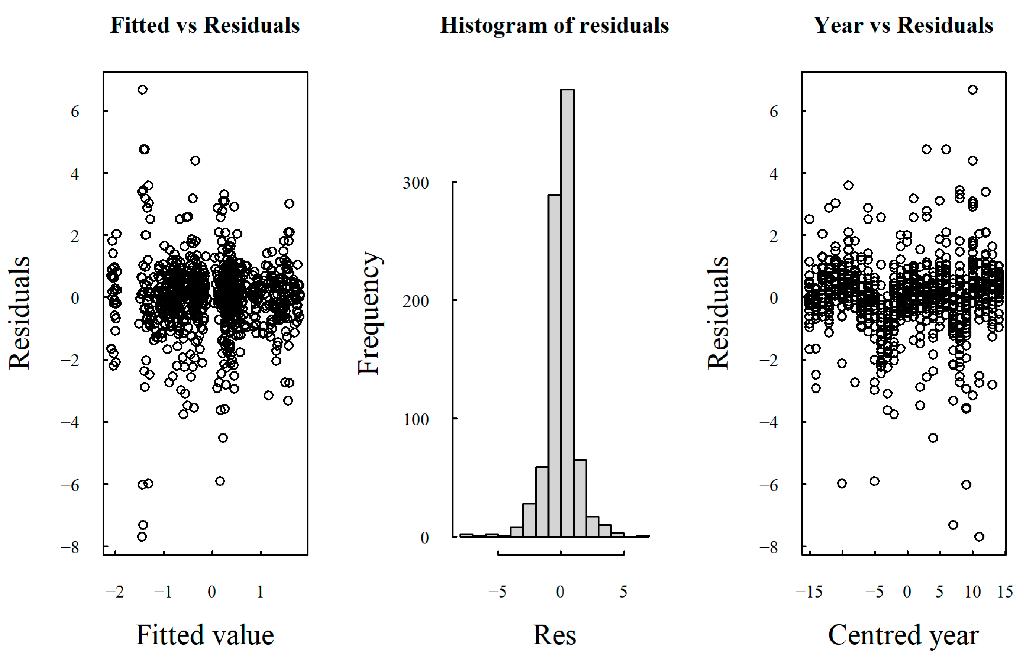
Fixed effects: The fixed effects show that the time variable has no significant influence on the standardized log(APIn) value (see Table A2). Likewise, the intercept is not significantly different from zero. Therefore, no consistent overall trend can be detected across taxa.
Table A2.
Results of the model selection procedure for the fixed effect of the taxon-specific model.
Random effects: The variance of the random intercept (SD = 0.91) indicates substantial differences in mean log(APIn) values among taxa at the central point of the time series. In contrast, the variance of the temporal slopes is very small (SD slope = 0.01), suggesting that only minor differences in temporal trends among species; however, these are estimated in logarithmic units. The correlation between the random intercept and slope is r = –0.07, indicating that the two are largely independent. The residual variance within groups is 0.40, reflecting a moderate amount of unexplained variation within species. As the log(APIn) values were standardised, the residual variance can be interpreted directly as a standard deviation, a value of 0.40 is smaller than 1, indicating moderate within-group variability. Thus, the model captures some of the variation through fixed effects (time) and random effects (species), but some residual variation within groups remains unexplained.
Taxon-specific model parameters: The random-intercept and random-slope model enables estimation of taxon-specific intercepts Log10(APInYrav), representing log10(APIn) at the mean year of the study period, and taxon-specific slopes Log10(β(Yr − Yrav)), representing log10-standardised annual changes. Both estimates are reported for each taxon in Table A3. Taxon-specific conditional estimates of the slopes are additionally shown in Figure 4 (Main Text) to illustrate the heterogeneity of temporal trends among taxa. As these estimates arise from the random-effects structure of the mixed-effects model, they are not subject to separate hypothesis tests and therefore do not have associated individual p-values. Statistical inference is instead based on the estimated variance of the random slopes and on model comparisons which evaluates whether the inclusion of taxon-specific slopes improves the model’s fit.
To facilitate the interpretation of the model results, all the standardised coefficients were converted back into the original APIn units [Pollen * day/m3]. First, the standardized intercept (Log10(APInYrav)) and slope (Log10(β(Yr − Yrav))) estimates were converted back to the scale of the log-transformed APIn values by reversing the centering transformation using the mean and standard deviation of Log10(APIn). The intercept on the log scale was then exponentiated to obtain the corresponding APIn value on the original scale (APInYrav).
The slope on the log scale represents the proportional annual change in APIn. Therefore, the absolute annual change in APIn (β(Yr − Yrav)) was obtained by multiplying the back-transformed intercept by the slope on the log scale. Finally, the relative annual change ΔAPIn [%Yr−1] was expressed as a percentage by multiplying the slope on the log-scale by 100.
Table A3.
Estimates of the taxon-specific intercept and slopes.
Appendix A.3. Results of the Model Selection Procedure—Ecological Categories
We then used the model with the best-supported random and correlation structure to investigate the presence of trends across ecological categories (distribution area and growth forms).
Table A4 presents the results of the model selection procedure used to evaluate the significance of adding the fixed effects growth form to the model described in Equation (A3). For clarity, we do not report the random structure, as it remains unchanged from this point of the analysis onward.
Table A4.
Results of the model selection procedure for the fixed effects of the growth form model.
In this model selection procedure, we first tested whether adding a fixed effect to the intercept (model 4) by including the additive term growth form improved model performance. This increase in model complexity was not supported by a better fit to the data (AIC = 1046.06; BIC = 1084.15; logLik = −515.03; p-value = 0.11). We therefore discarded the additive term and proceeded with a model using a slope-only parametrization for growth form (model 5). This increase in model complexity was supported by a better fit to the data (AIC = 1043.11; BIC = 1081.20; logLik = −513.56; p-value = 0.02), so we retained this parameter in the model. Finally, we tested whether including an interaction between the intercept and the slope (model 6) would further improve model’s performance. However, this additional increase in model complexity was not supported by a better fit to the data (AIC = 1043.36; BIC = 1086.21; logLik = −512.68; p-value = 0.19).
The absence of violations of model assumptions and temporal autocorrelation was visually validated (Figure A2), and the best-fitting growth form model (model 5) was subsequently refitted using restricted maximum likelihood (REML).
Figure A2.
Visual check of model assumption violations for the best-fitting growth-form model.
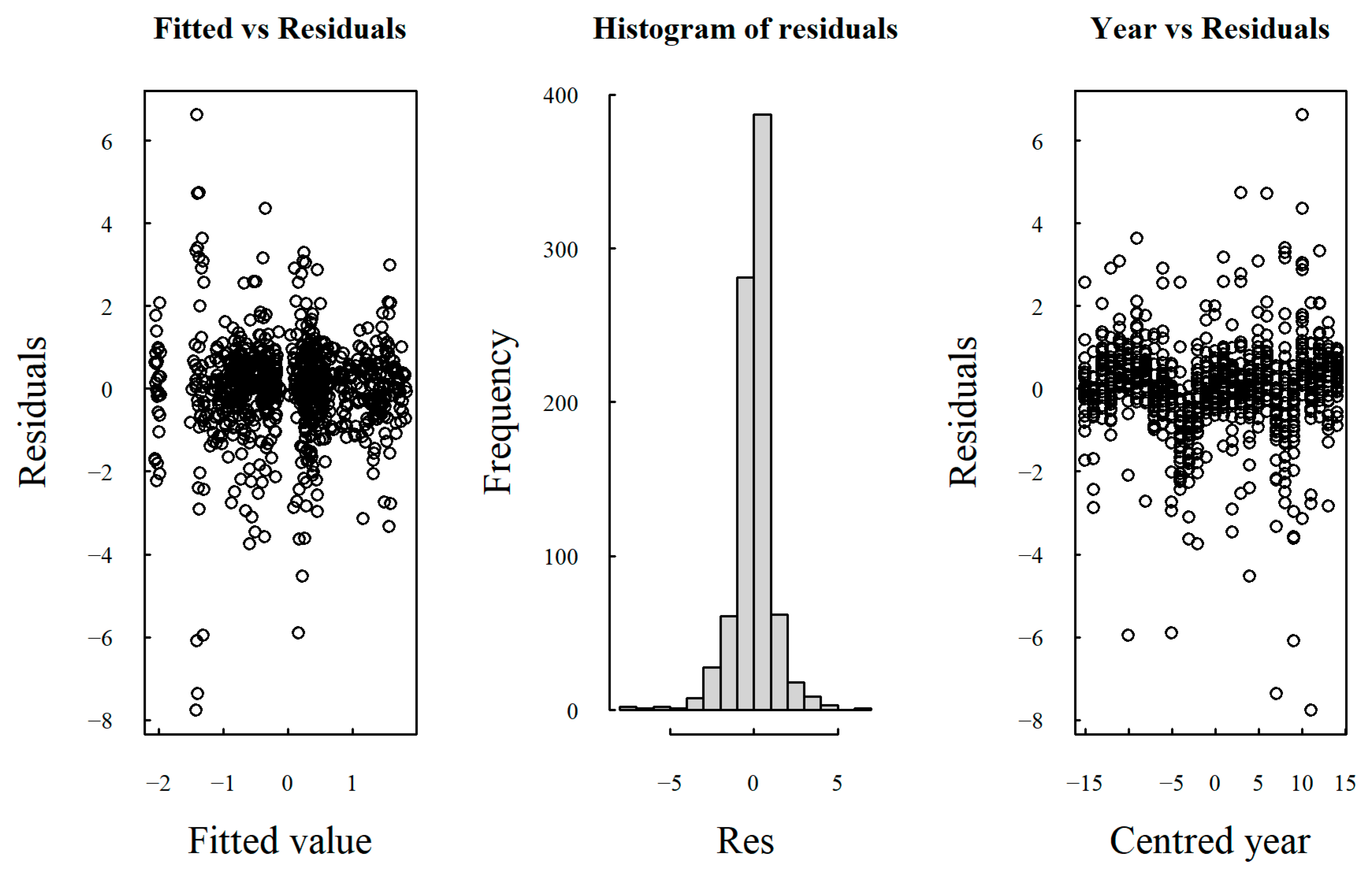
Table A5 reports the parameter estimates for the fixed effect of the best-fitting growth-form model.
Table A5.
Parameter estimates for the best fitting growth-form model.
Fixed effects: The fixed effects indicate a significant positive influence of the time variable on the standardised log(APIn) values for the arboreal growth form only. There is no evidence for temporal changes in log(APIn) within the non-arboreal growth form. The intercept is likewise not significantly different from zero.
Table A6 presents the results of the model selection procedure used to evaluate the significance of adding the distribution area fixed effects to the model described in Equation (A3).
Table A6.
Results of the model selection procedure for the fixed effects of the distribution area model.
In this model selection procedure, we first tested whether adding a fixed effect to the intercept (model 7) by including the additive term distribution area improved the model’s performance. This increase in model complexity was supported by a better fit to the data (AIC = 1044.71; BIC = 1082.80; logLik = −514.35; p-value = 0.05). We then proceeded to a model using a slope-only parametrization for the distribution area (model 8). This further increase in model complexity was also supported by an improved fit to the data (AIC = 1042.80; BIC = 1080.90; logLik = −513.40; p-value = 0.02). We therefore retained both parameters in the final model. Then we finally tested whether including an interaction between intercept and slope (model 9) would further improve the model’s performance. This additional increase in model complexity was supported by a better fit to the data (AIC = 1040.95; BIC = 1083.80; logLik = −511.47; p-value = 0.05).
The absence of violations of model assumptions and temporal autocorrelation was visually validated, and the best-fitting distribution area model (model 9, Figure A3) was subsequently refitted using restricted maximum likelihood (REML).
Figure A3.
Visual check of the model assumption violations for the best-fitting distribution area model.
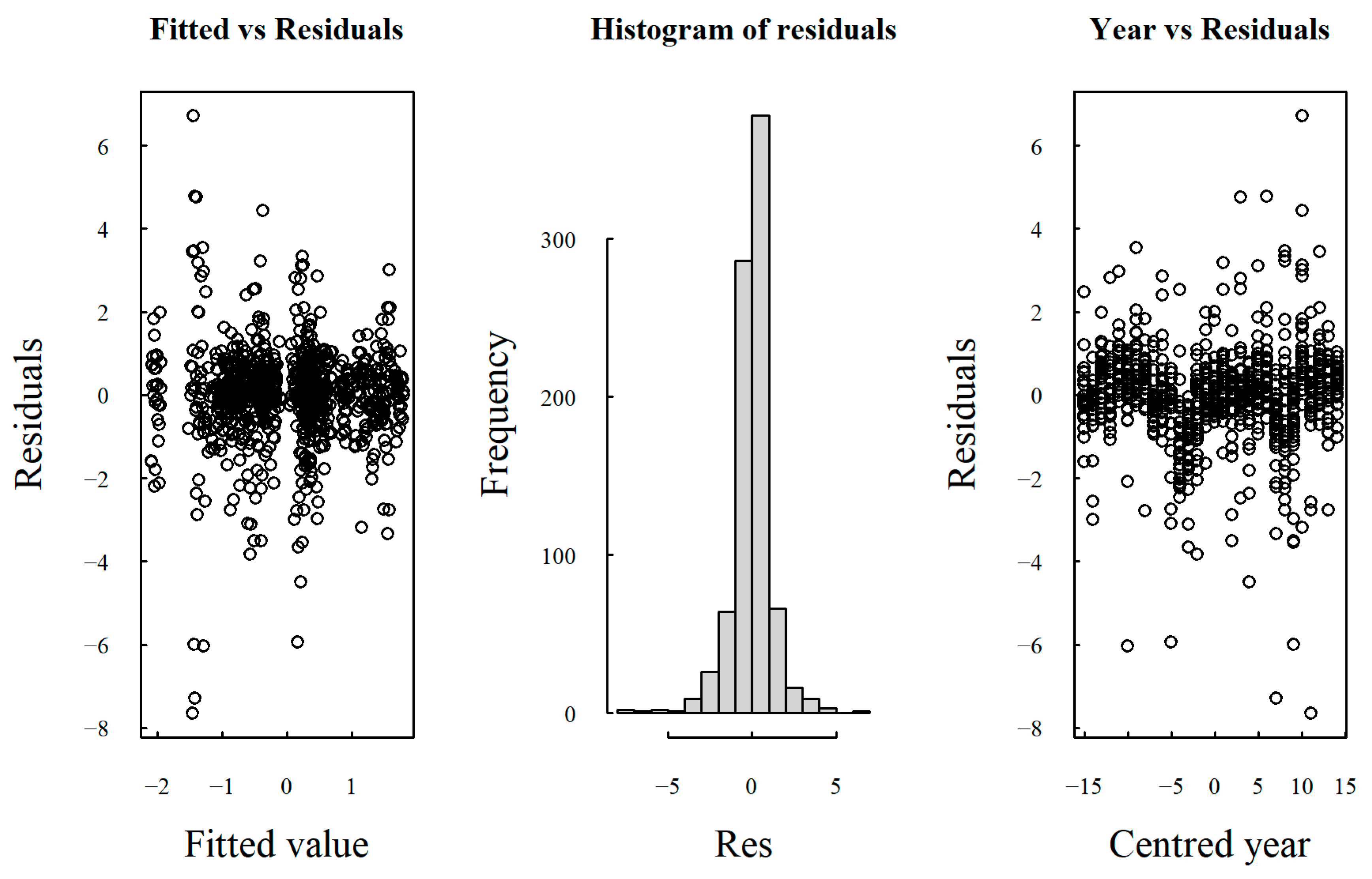
Table A7 reports the parameter estimates for the fixed-effect of the best-fitting distribution area model.
Table A7.
Parameter estimates for the best fitting distribution area model.
Fixed effects: The fixed effects indicate a significant positive influence of the time variable on standardised log(APIn) values for taxa with a non-native distribution area, whereas there is no evidence of temporal changes in log(APIn) for native taxa. The intercept for native taxa is likewise not significantly different from zero, whereas the intercept for non-native taxa is significantly lower than that of native taxa.
References
- Beggs, P.J.; Clot, B.; Sofiev, M.; Johnston, F.H. Climate Change, Airborne Allergens, and Three Translational Mitigation Approaches. eBioMedicine 2023, 93, 104478. [Google Scholar] [CrossRef] [Scilit] [PubMed]
- D’Amato, G.; Chong-Neto, H.J.; Monge Ortega, O.P.; Vitale, C.; Ansotegui, I.; Rosario, N.; Haahtela, T.; Galán, C.; Pawankar, R.; Murrieta-Aguttes, M.; et al. The Effects of Climate Change on Respiratory Allergy and Asthma Induced by Pollen and Mold Allergens. Allergy 2020, 75, 2219–2228. [Google Scholar] [CrossRef] [Scilit] [PubMed]
- Adams-Groom, B.; Selby, K.; Derrett, S.; Frisk, C.A.; Pashley, C.H.; Satchwell, J.; King, D.; McKenzie, G.; Neilson, R. Pollen Season Trends as Markers of Climate Change Impact: Betula, Quercus and Poaceae. Sci. Total Environ. 2022, 831, 154882. [Google Scholar] [CrossRef] [Scilit] [PubMed]
- Dierick, B.J.H.; van der Molen, T.; Flokstra-de Blok, B.M.J.; Muraro, A.; Postma, M.J.; Kocks, J.W.H.; van Boven, J.F.M. Burden and Socioeconomics of Asthma, Allergic Rhinitis, Atopic Dermatitis and Food Allergy. Expert Rev. Pharmacoecon. Outcomes Res. 2020, 20, 437–453. [Google Scholar] [CrossRef] [Scilit] [PubMed]
- World Health Organization. Climate Change, Air Pollution, Pollen and Health: Technical Brief; WHO Air Quality; Energy and Health Science and Policy Summaries; World Health Organization: Geneva, Switzerland, 2025. [Google Scholar] [CrossRef] [Scilit]
- Ziska, L.H.; Makra, L.; Harry, S.K.; Bruffaerts, N.; Hendrickx, M.; Coates, F.; Saarto, A.; Thibaudon, M.; Oliver, G.; Damialis, A.; et al. Temperature-Related Changes in Airborne Allergenic Pollen Abundance and Seasonality across the Northern Hemisphere: A Retrospective Data Analysis. Lancet Planet. Health 2019, 3, e124–e131. [Google Scholar] [CrossRef] [Scilit] [PubMed]
- Tagliaferro, S.; Marchetti, P.; Dall’Ara, B.; Domenichini, F.; Lazzarin, S.; Nicolis, M.; Selle, D.; Silibello, C.; Marcon, A. Temporal Trends of Seasonal Pollen Indexes in a Region of Northern Italy (2001–2022). Atmos. Environ. 2024, 338, 120826. [Google Scholar] [CrossRef] [Scilit]
- Agache, I.; Torres, M.; Eguiluz-Gracia, I.; Bradatan, E.; El Abd, K.; Bilo, M.B.; Rivolta, F.; Sangalli, A.; Bumbacea, R.; Ali, S.; et al. Economic Impact of Allergic Diseases and Asthma—The HEAD Pan-European Registry. Allergy 2025, 80, 1677–1701. [Google Scholar] [CrossRef] [Scilit] [PubMed]
- Pereira, A.M.; De Linares, C.; Belmonte, J. Aerobiological Modeling I: A Review of Predictive Models. Sci. Total Environ. 2021, 795, 148783. [Google Scholar] [CrossRef] [Scilit] [PubMed]
- Dirr, L.; Bouchal, J.M.; Berger, M.; Marquer, L.; Döllinger, T.; Harvey, P.; Berger, U.E. European Aeroallergen Network (EAN): A Key Tool to Analyze the Birch Pollen Season in Europe. Allergo J. Int. 2025, 35, 158–167. [Google Scholar] [CrossRef] [Scilit]
- ISPRA. POLLnet–Rete Italiana di Monitoraggio Aerobiologico. Available online: https://pollnet.isprambiente.it (accessed on 21 August 2026).
- ISPRA. Pollini Allergenici in Italia: Analisi dei Trend 2010–2019; Rapporto ISPRA 335/2020; ISPRA: Rome, Italy, 2020; ISBN 978-88-448-1033-7. Available online: https://www.isprambiente.gov.it/it/pubblicazioni/rapporti/pollini-allergenici-in-italia-analisi-dei-trend-2010-2019 (accessed on 21 August 2026).
- Buters, J.T.M.; Antunes, C.; Galveias, A.; Bergmann, K.C.; Thibaudon, M.; Galán, C.; Schmidt-Weber, C.; Oteros, J. Pollen and Spore Monitoring in the World. Clin. Transl. Allergy 2018, 8, 9. [Google Scholar] [CrossRef] [Scilit] [PubMed]
- Biologisches Labor der Landesagentur für Umwelt und Klimaschutz der Autonomen Provinz Bozen—Südtirol. Polleninformationsdienst Südtirol. Available online: https://umwelt.provinz.bz.it/de/luft/polleninformationsdienst-suedtirol (accessed on 21 August 2026).
- Cristofolini, F.; Anelli, P.; Billi, B.M.; Bocchi, C.; Borney, M.F.; Bucher, E.; Cassoni, F.; Coli, S.; De Gironimo, V.; Gottardini, E.; et al. Temporal Trends in Airborne Pollen Seasonality: Evidence from the Italian POLLnet Network Data. Aerobiologia 2020, 36, 63–70. [Google Scholar] [CrossRef] [Scilit]
- Bonini, M.; Cardarelli, E.; Faccini, M.; Sofiev, M.; Palamarchuk, J.; Pelagatti, M.M.; Monti, G.S. Effects of Climate Change on Pollen Season Features of Herbaceous Species in the Milan Area, Northern Italy. Sci. Rep. 2026, 16, 11260. [Google Scholar] [CrossRef] [Scilit] [PubMed]
- Gehrig, R.; Clot, B. 50 Years of Pollen Monitoring in Basel (Switzerland) Demonstrate the Influence of Climate Change on Airborne Pollen. Front. Allergy 2021, 2, 677159. [Google Scholar] [CrossRef] [Scilit] [PubMed]
- Rojo, J.; Picornell, A.; Oteros, J.; Werchan, M.; Werchan, B.; Bergmann, K.-C.; Smith, M.; Weichenmeier, I.; Schmidt-Weber, C.B.; Buters, J. Consequences of Climate Change on Airborne Pollen in Bavaria, Central Europe. Reg. Environ. Change 2021, 21, 9. [Google Scholar] [CrossRef] [Scilit]
- Albertini, R.; Coluccia, A.; Mohieldin Mahgoub Ibrahim, M.; Colucci, M.E.; Zoni, R.; Affanni, P.Q.; Veronesi, L.; Pasquarella, C. The Impact of Climate Change on the Spread of Airborne Pollen in Northern Italy—The Results of 27 Years of Monitoring in Parma. Preprints 2025, 2025011624. [Google Scholar] [CrossRef] [Scilit]
- Choi, Y.-J.; Lee, K.S.; Oh, J.-W. The Impact of Climate Change on Pollen Season and Allergic Sensitization to Pollens. Immunol. Allergy Clin. N. Am. 2021, 41, 97–109. [Google Scholar] [CrossRef] [Scilit] [PubMed]
- Kim, K.R.; Oh, J.-W.; Woo, S.-Y.; Seo, Y.A.; Choi, Y.-J.; Kim, H.S.; Lee, W.Y.; Kim, B.-J. Does the Increase in Ambient CO2 Concentration Elevate Allergy Risks Posed by Oak Pollen? Int. J. Biometeorol. 2018, 62, 1587–1594. [Google Scholar] [CrossRef] [Scilit] [PubMed]
- Schinko, H.A.E.; Lamprecht, B.; Schmidt, R. How Will Climate Change Alter the Dynamics of Airborne Pollen and Pollen Load of Allergenic Plants?: The “Exceptionally Warm Year” 2018 in Linz (Upper Austria)—A Potential Model for the Future Based on Long-Term Trends. Allergo J. Int. 2021, 30, 96–108. [Google Scholar] [CrossRef] [Scilit]
- De Weger, L.A.; Bruffaerts, N.; Koenders, M.M.J.F.; Verstraeten, W.W.; Delcloo, A.W.; Hentges, P.; Hentges, F. Long-Term Pollen Monitoring in the Benelux: Evaluation of Allergenic Pollen Levels and Temporal Variations of Pollen Seasons. Front. Allergy 2021, 2, 676176. [Google Scholar] [CrossRef] [Scilit] [PubMed]
- Cristofolini, F.; Cristofori, A.; Corradini, S.; Gottardini, E. The Impact of Temperature on Increased Airborne Pollen and Earlier Onset of the Pollen Season in Trentino, Northern Italy. Reg. Environ. Change 2024, 24, 60. [Google Scholar] [CrossRef] [Scilit]
- Besancenot, J.-P.; Mascarell, L. Climate-Driven Changes in Pollen Dynamics: Increased Loads and Earlier, Longer Exposure. Explor Asthma Allergy 2026, 4, 1009107. [Google Scholar] [CrossRef] [Scilit]
- Damialis, A.; Traidl-Hoffmann, C.; Treudler, R. Climate Change and Pollen Allergies. In Biodiversity and Health in the Face of Climate Change; Marselle, M.R., Stadler, J., Korn, H., Irvine, K.N., Bonn, A., Eds.; Springer International Publishing: Cham, Switzerland, 2019; pp. 47–66. ISBN 978-3-030-02317-1. [Google Scholar]
- Ziska, L.H.; Beggs, P.J. Anthropogenic Climate Change and Allergen Exposure: The Role of Plant Biology. J. Allergy Clin. Immunol. 2012, 129, 27–32. [Google Scholar] [CrossRef] [Scilit] [PubMed]
- Knolmajer, B.; Jócsák, I.; Taller, J.; Keszthelyi, S.; Kazinczi, G. Common Ragweed—Ambrosia artemisiifolia L.: A Review with Special Regards to the Latest Results in Biology and Ecology. Agronomy 2024, 14, 497. [Google Scholar] [CrossRef] [Scilit]
- Stawoska, I.; Myszkowska, D.; Oliwa, J.; Skoczowski, A.; Wesełucha-Birczyńska, A.; Saja-Garbarz, D.; Ziemianin, M. Air Pollution in the Places of Betula Pendula Growth and Development Changes the Physicochemical Properties and the Main Allergen Content of Its Pollen. PLoS ONE 2023, 18, e0279826. [Google Scholar] [CrossRef] [Scilit] [PubMed]
- D’Amato, G.; Cecchi, L.; D’Amato, M.; Liccardi, G. Urban Air Pollution and Climate Change as Environmental Risk Factors of Respiratory Allergy: An Update. J. Investig. Allergol. Clin. Immunol. 2010, 20, 95–102. [Google Scholar] [PubMed]
- Beck, I.; Jochner, S.; Gilles, S.; McIntyre, M.; Buters, J.T.M.; Schmidt-Weber, C.; Behrendt, H.; Ring, J.; Menzel, A.; Traidl-Hoffmann, C. High Environmental Ozone Levels Lead to Enhanced Allergenicity of Birch Pollen. PLoS ONE 2013, 8, e80147. [Google Scholar] [CrossRef] [Scilit] [PubMed]
- Gentili, R.; Gilardelli, F.; Bona, E.; Prosser, F.; Selvaggi, A.; Alessandrini, A.; Martini, F.; Nimis, P.L.; Wilhalm, T.; Adorni, M.; et al. Distribution Map of Ambrosia artemisiifolia L. (Asteraceae) in Italy. Plant Biosyst. Int. J. Deal. All Asp. Plant Biol. 2017, 151, 381–386. [Google Scholar] [CrossRef] [Scilit]
- Cristofori, A.; Bucher, E.; Rossi, M.; Cristofolini, F.; Kofler, V.; Prosser, F.; Gottardini, E. The Late Flowering of Invasive Species Contributes to the Increase of Artemisia Allergenic Pollen in Autumn: An Analysis of 25 Years of Aerobiological Data (1995–2019) in Trentino-Alto Adige (Northern Italy). Aerobiologia 2020, 36, 669–682. [Google Scholar] [CrossRef] [Scilit]
- Pecoraro, L.; Giovannini, M.; Mori, F.; Barni, S.; Castagnoli, R.; Arasi, S.; Mastrorilli, C.; Saretta, F.; Liotti, L.; Caminiti, L.; et al. Imported Allergens in Italy: An Emerging Issue. Ital. J. Pediatr. 2024, 50, 36. [Google Scholar] [CrossRef] [Scilit] [PubMed]
- Cariñanos, P.; Grilo, F.; Pinho, P.; Casares-Porcel, M.; Branquinho, C.; Acil, N.; Andreucci, M.B.; Anjos, A.; Bianco, P.M.; Brini, S.; et al. Estimation of the Allergenic Potential of Urban Trees and Urban Parks: Towards the Healthy Design of Urban Green Spaces of the Future. Int. J. Environ. Res. Public Health 2019, 16, 1357. [Google Scholar] [CrossRef] [Scilit] [PubMed]
- Ziello, C.; Sparks, T.H.; Estrella, N.; Belmonte, J.; Bergmann, K.C.; Bucher, E.; Brighetti, M.A.; Damialis, A.; Detandt, M.; Galán, C.; et al. Changes to Airborne Pollen Counts across Europe. PLoS ONE 2012, 7, e34076. [Google Scholar] [CrossRef] [Scilit] [PubMed]
- Cariñanos, P.; Marinangeli, F. An Updated Proposal of the Potential Allergenicity of 150 Ornamental Trees and Shrubs in Mediterranean Cities. Urban For. Urban Green. 2021, 63, 127218. [Google Scholar] [CrossRef] [Scilit]
- Pfattner, M.; Eschgfäller, M. Trachtkalender Südtirol; Autonome Provinz Bozen—Südtirol; Land-und Forstwirtschaftliches Versuchszentrum Laimburg: Bozen, Italy, 2010. [Google Scholar]
- Zebisch, M.; Vaccaro, R.; Niedrist, G.; Schneiderbauer, S.; Streifeneder, T.P.; Weiß, M.L.; Troi, A.; Renner, K.; Pedoth, L.; Baumgartner, B.; et al. Klimareport Südtirol 2018; Eurac Research: Bozen/Bolzano, Italy, 2018; Available online: https://bia.unibz.it/esploro/outputs/report/Klimareport-Sudtirol-2018/991005773136901241/filesAndLinks?index=0 (accessed on 21 August 2026).
- ASTAT—Landesinstitut für Statistik der Autonomen Provinz Bozen—Südtirol. Bevölkerungsentwicklung (vorläufige Daten)—2025. Available online: https://astat.provinz.bz.it/de/bevoelkerung (accessed on 21 August 2026).
- Rubel, F.; Brugger, K.; Haslinger, K.; Auer, I. The Climate of the European Alps: Shift of Very High Resolution Köppen-Geiger Climate Zones 1800–2100. metz 2017, 26, 115–125. [Google Scholar] [CrossRef] [Scilit]
- Adler, S.; Chimani, B.; Drechsel, S.; Haslinger, K.; Hiebl, J.; Meyer, V.; Resch, G.; Rudolph, J.; Vergeiner, J.; Zingerle, C.; et al. Das Klima von Tirol–Südtirol–Belluno: Vergangenheit–Gegenwart–Zukunft; Zentralanstalt für Meteorologie und Geodynamik (ZAMG), Abteilung Brand- und Zivilschutz der Autonomen Provinz Bozen—Südtirol and Agenzia Regionale per la Prevenzione e Protezione Ambientale del Veneto (ARPAV): Vienna, Austria, 2015; Available online: https://www.provinz.bz.it/wetter/download/Das_Klima_von_Tirol-Suedtirol-Belluno.pdf (accessed on 21 August 2026).
- Amt für Meteorologie und Lawinenwarnung der Autonomen Provinz Bozen—Südtirol. Monats- und Jahres Niederschläge [mm] von Bozen. Available online: https://view.officeapps.live.com/op/view.aspx?src=https%3A%2F%2Fstatic-wetter.provinz.bz.it%2Fweb-data%2Fmeasurment-data%2F83200MS-Bozen-Bolzano-multiannual-N-monthly-precipitation.xlsx&wdOrigin=BROWSELINK (accessed on 21 August 2026).
- CORINE Land Cover 2018 (Vector/Raster 100 m), Europe, 6-Yearly. Available online: https://land.copernicus.eu/en/products/corine-land-cover/clc2018 (accessed on 21 August 2026).
- Peer, T. Karte der aktuellen Vegetation Südtirols 1/100 000 Blatt Bozen—Carta della vegetazione attuale del Sudtirolo Foglio Bolzano. Doc. Cartogr. Écol. 1980, 23, 25–46. [Google Scholar]
- Dalla Fior, G. La nostra flora: Guida alla conoscenza della flora della regione Trentino–Alto Adige, 3rd ed.; G.B. Monauni: Trento, Italy, 1969. [Google Scholar]
- PalDat. Available online: https://www.paldat.org/ (accessed on 21 August 2026).
- Bucher, E.; Kofler, V.; Vorwohl, G.; Zieger, E. Das Pollenbild der Südtiroler Honige; Landesagentur für Umwelt und Klimaschutz; Biologisches Labor: Bolzano, Italy, 2004. [Google Scholar]
- Smith, E.G. Sampling and Identifying Allergenic Pollens and Molds: An Illustrated Identification Manual for Air Samplers; Blewstone Press: San Antonio, TX, USA, 1990; ISBN 0-930961-02-1. [Google Scholar]
- Feliziani, V. Pollini Di Interesse Allergologico: Guida al Loro Riconoscimento; Masson Italia Editori S.p.A.: Milano, Italy, 1986. [Google Scholar]
- UNI EN 16868:2019; Aria Ambiente—Campionamento ed Analisi di Pollini e Spore Fungine Dispersi in Aria per le Reti di Monitoraggio delle Allergie—Metodo Volumetrico Hirst. UNI—Ente Italiano di Normazione: Milan, Italy, 2019.
- Rojo, J.; Picornell, A.; Oteros, J. AeRobiology: The Computational Tool for Biological Data in the Air. Methods Ecol. Evol. 2019, 10, 1371–1376. [Google Scholar] [CrossRef] [Scilit]
- FloraFaunaSüdtirol. Das Portal zur Verbreitung von Tier- und Pflanzenarten in Südtirol; Naturmuseum Südtirol: Bozen, Italy, 2014; Available online: https://www.florafauna.it/portal/index (accessed on 21 August 2026).
- Wilhalm, T.; Niklfeld, H.; Gutermann, W. Katalog der Gefäßpflanzen Südtirols; Veröffentlichungen des Naturmuseums Südtirol. 3; Folio Verlag: Wien, Austria; Bozen, Italy, 2006; ISBN 978-3-85256-325-1. [Google Scholar]
- D’Amato, G.; Ruffilli, A.; Sacerdoti, G.; Bonini, S. Parietaria Pollinosis: A Review. Allergy 1992, 47, 443–449. [Google Scholar] [CrossRef] [Scilit] [PubMed]
- Pinheiro, J.; Bates, D. Mixed-Effects Models in S and S-PLUS; Springer: New York, NY, USA, 2000; ISBN 0-387-98957-9. [Google Scholar]
- Pinheiro, J.; Bates, D.; R Core Team. nlme: Linear and Nonlinear Mixed Effects Models. R Package Version 3.1-170. 2026. Available online: https://CRAN.R-project.org/package=nlme (accessed on 21 August 2026).
- Zuur, A.; Ieno, E.; Walker, N.; Saveliev, A.; Smith, G. Mixed Effects Models and Extensions in Ecology with R; Springer: New York, NY, USA, 2009; ISBN 978-0-387-87457-9. [Google Scholar]
- Nilsson, S.; Persson, S. Tree Pollen Spectra in the Stockholm Region (Sweden), 1973–1980. Grana 1981, 20, 179–182. [Google Scholar] [CrossRef] [Scilit]
- Bastl, K.; Kmenta, M.; Berger, U.E. Defining Pollen Seasons: Background and Recommendations. Curr. Allergy Asthma Rep. 2018, 18, 73. [Google Scholar] [CrossRef] [Scilit] [PubMed]
- Negrini, A.C.; Negrini, S.; Giunta, V.; Quaglini, S.; Ciprandi, G. Thirty-Year Survey on Airborne Pollen Concentrations in Genoa, Italy: Relationship with Sensitizations, Meteorological Data, and Air Pollution. Am. J. Rhinol. Allergy 2011, 25, e232–e241. [Google Scholar] [CrossRef] [Scilit] [PubMed]
- Santucci, F.M.; Callieris, R. Organic Olive Oil in Italy: A Missed Opportunity? Bulg. J. Agric. Sci. 2021, 27, 1039–1050. [Google Scholar]
- Ciani, F.; Dell’Olmo, L.; Foggi, B.; Mariotti Lippi, M. The Effect of Urban Green Areas on Pollen Concentrations at Ground Level: A Study in the City of Florence (Italy). Urban For. Urban Green. 2021, 60, 127045. [Google Scholar] [CrossRef] [Scilit]
- Kudrnovsky, H.; Shaw, R.; Beckmann, B. Risk Assessment Template Developed Under the “Study on Invasive Alien Species—Development of Risk Assessments to Tackle Priority Species and Enhance Prevention”; Contract No. 07.0202/2019/812602/ETU/ENV.D.21; European Commission: Brussels, Belgium, 2022. [Google Scholar]
- De Weger, L.A.; Pashley, C.H.; Šikoparija, B.; Skjøth, C.A.; Kasprzyk, I.; Grewling, Ł.; Thibaudon, M.; Magyar, D.; Smith, M. The Long Distance Transport of Airborne Ambrosia Pollen to the UK and the Netherlands from Central and South Europe. Int. J. Biometeorol. 2016, 60, 1829–1839. [Google Scholar] [CrossRef] [Scilit] [PubMed]
- ARPA Friuli Venezia Giulia. Broussonetia Papyrifera: Indagine Sulla Diffusione in Italia nel 2021. Available online: https://www.arpa.fvg.it/temi/temi/pollini/ultimi-pubblicati/broussonetia-papyrifera-indagine-sulla-diffusione-in-italia-nel-2021/ (accessed on 21 August 2026).
- Cecchi, L.; Malaspina, T.T.; Albertini, R.; Zanca, M.; Ridolo, E.; Usberti, I.; Morabito, M.; Dall’ Aglio, P.; Orlandini, S. The Contribution of Long-Distance Transport to the Presence of Ambrosia Pollen in Central Northern Italy. Aerobiologia 2007, 23, 145–151. [Google Scholar] [CrossRef] [Scilit]
- De Franco, D.; Di Menno Di Bucchianico, A.; Travaglini, A.; Brighetti, M.A. Critical Issues of Aerobiological Monitoring: The Long-Distance Transport of Ambrosia Pollen into Rome. Aerobiology 2026, 4, 14. [Google Scholar] [CrossRef] [Scilit]
- Galán, C.; Smith, M.; Thibaudon, M.; Frenguelli, G.; Oteros, J.; Gehrig, R.; Berger, U.; Clot, B.; Brandao, R.; EAS QC Working Group. Pollen Monitoring: Minimum Requirements and Reproducibility of Analysis. Aerobiologia 2014, 30, 385–395. [Google Scholar] [CrossRef] [Scilit]
- ISPRA. POLLnet: Linee Guida per il Monitoraggio Aerobiologico; Manuali e Linee Guida 151/2017; ISPRA: Roma, Italy, 2017; 50p, ISBN 978-88-448-0820-4. [Google Scholar]
- Webservices des Südtiroler Polleninformationsdienstes. Open Data Portal der Landesagentur für Umwelt und Klimaschutz der Autonomen Provinz Bozen—Südtirol. Available online: https://data.civis.bz.it/ (accessed on 21 August 2026).
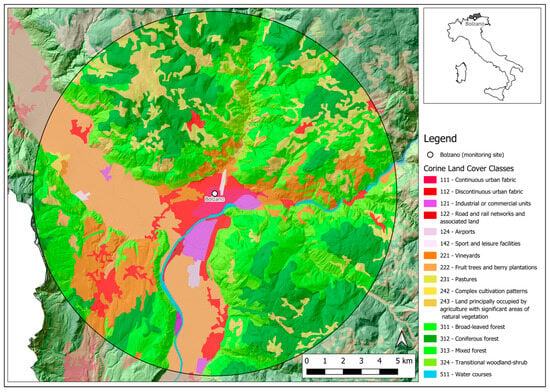
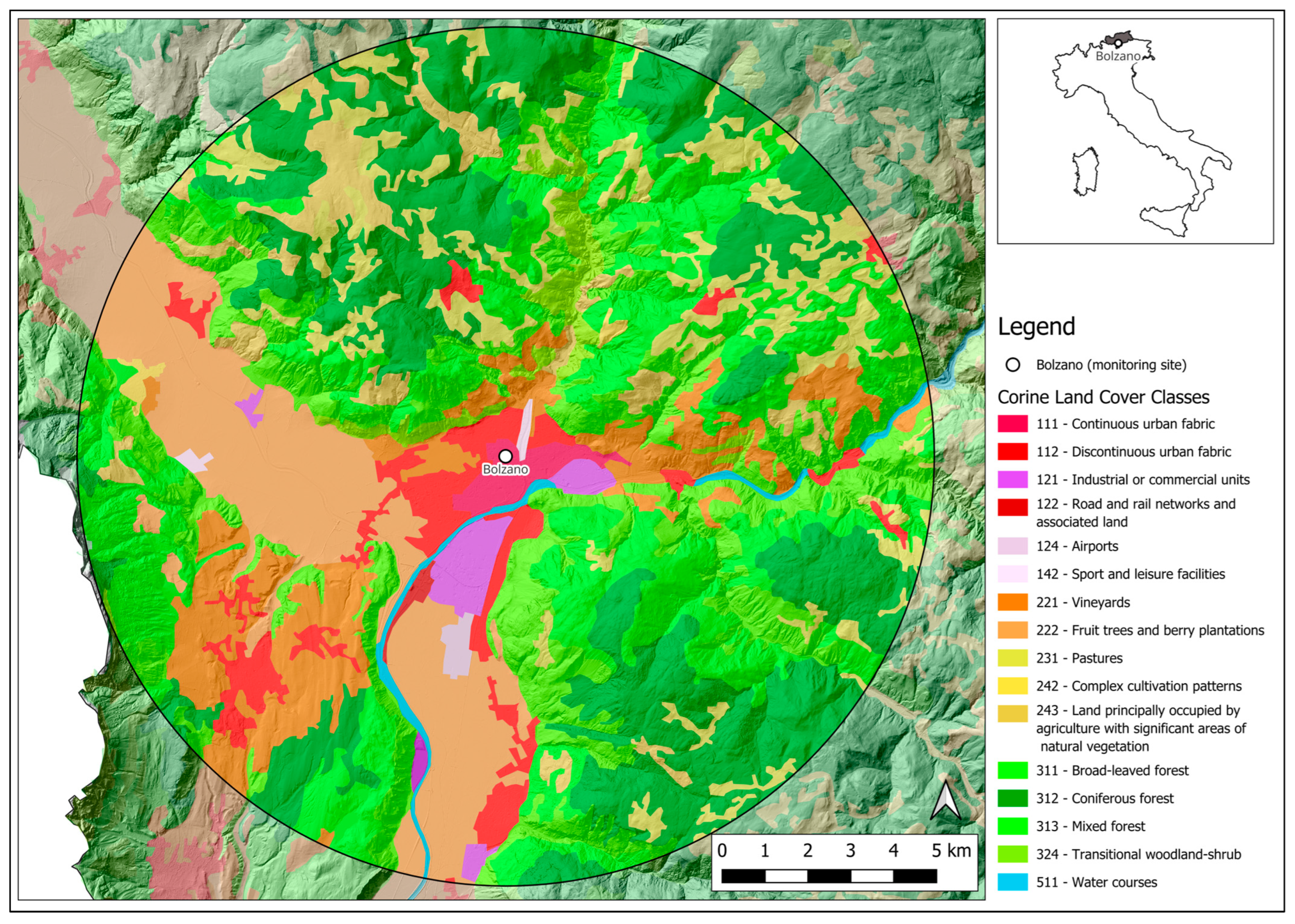
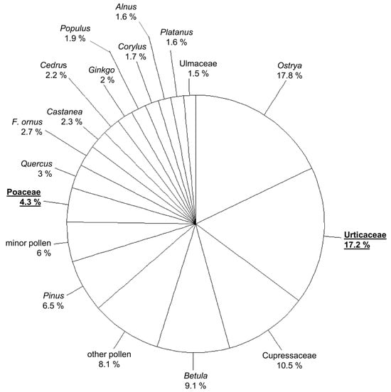
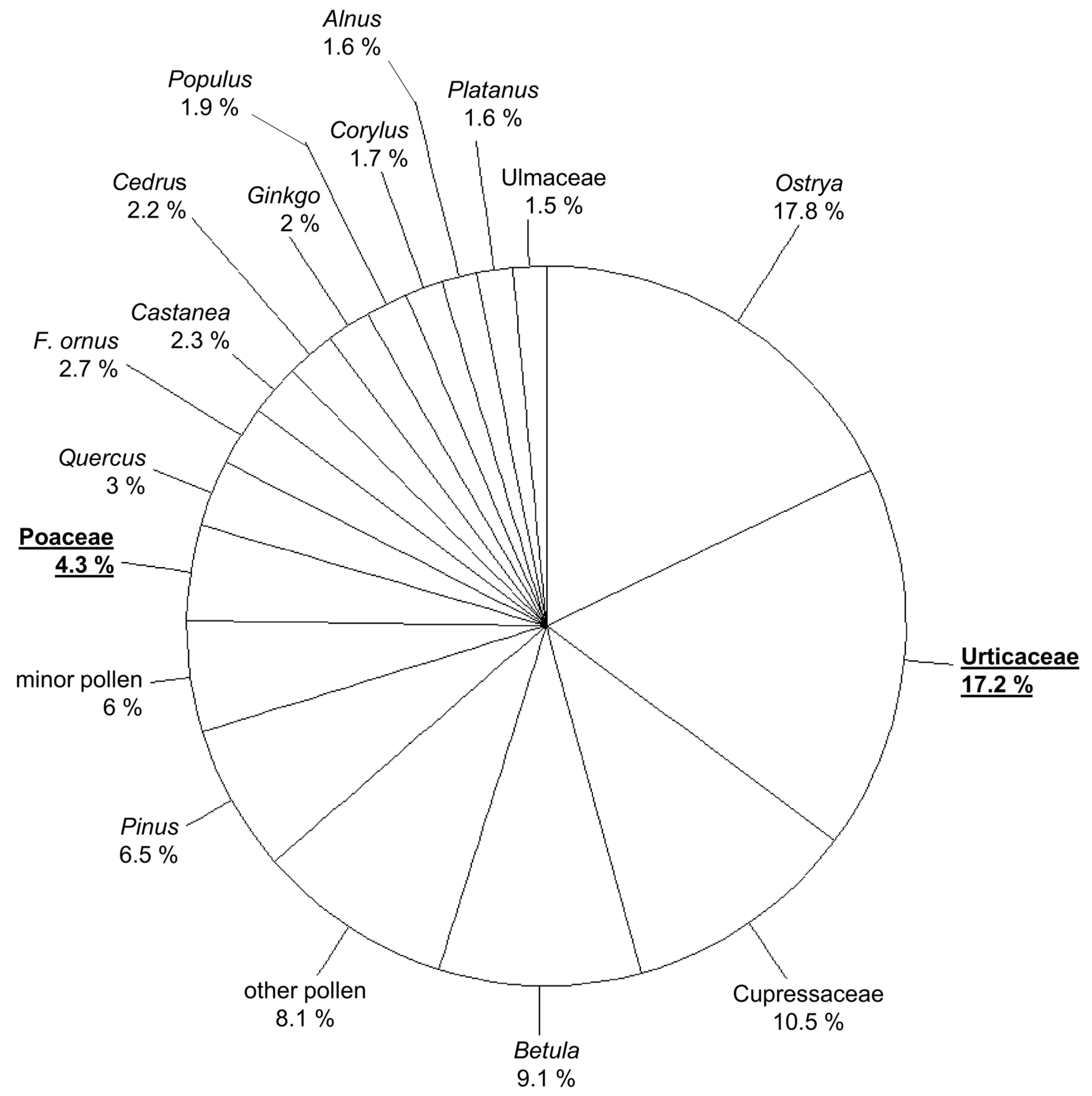
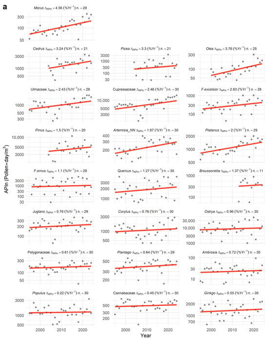
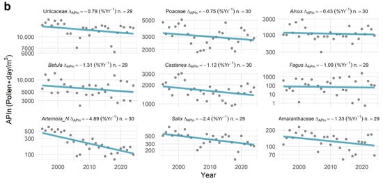
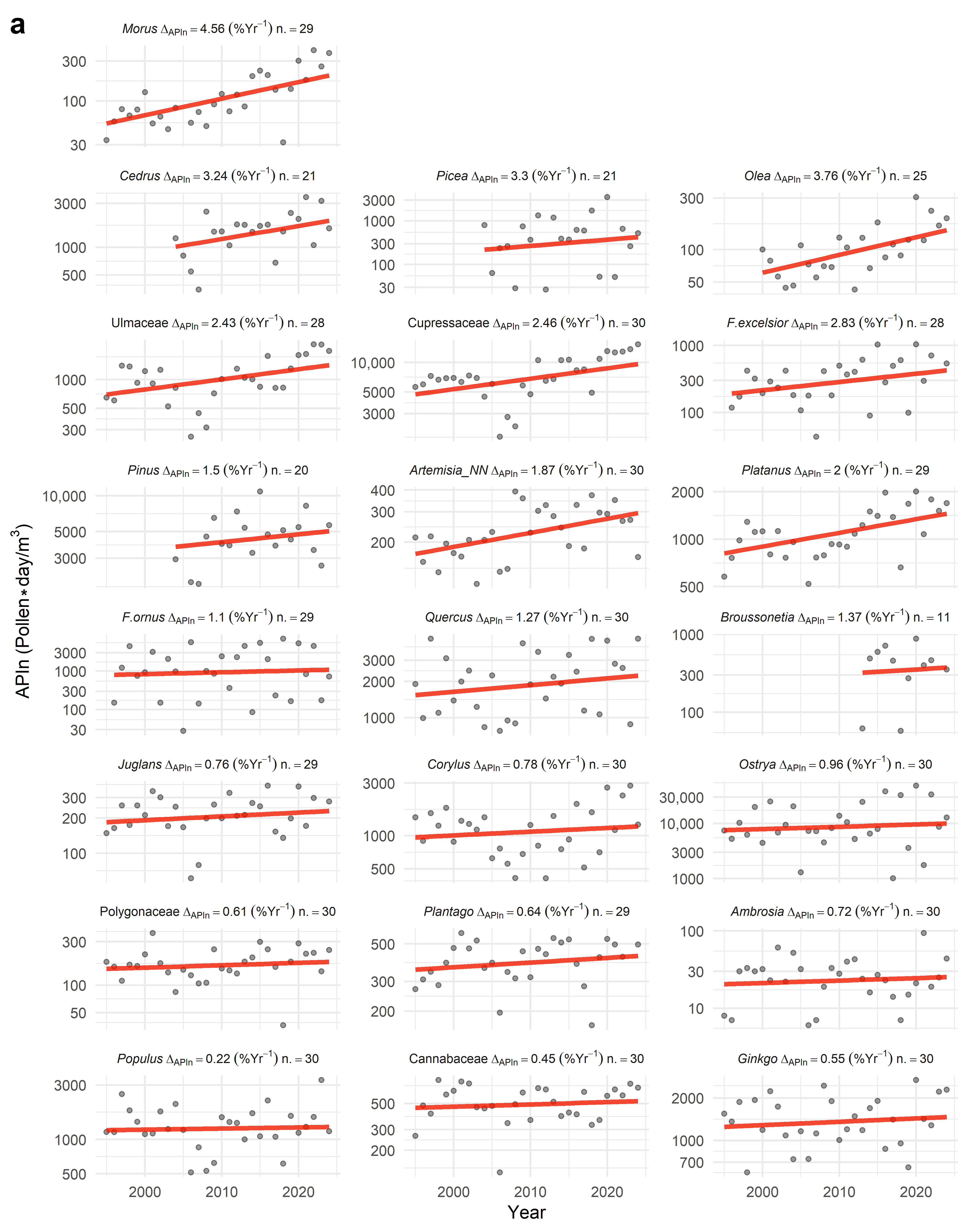
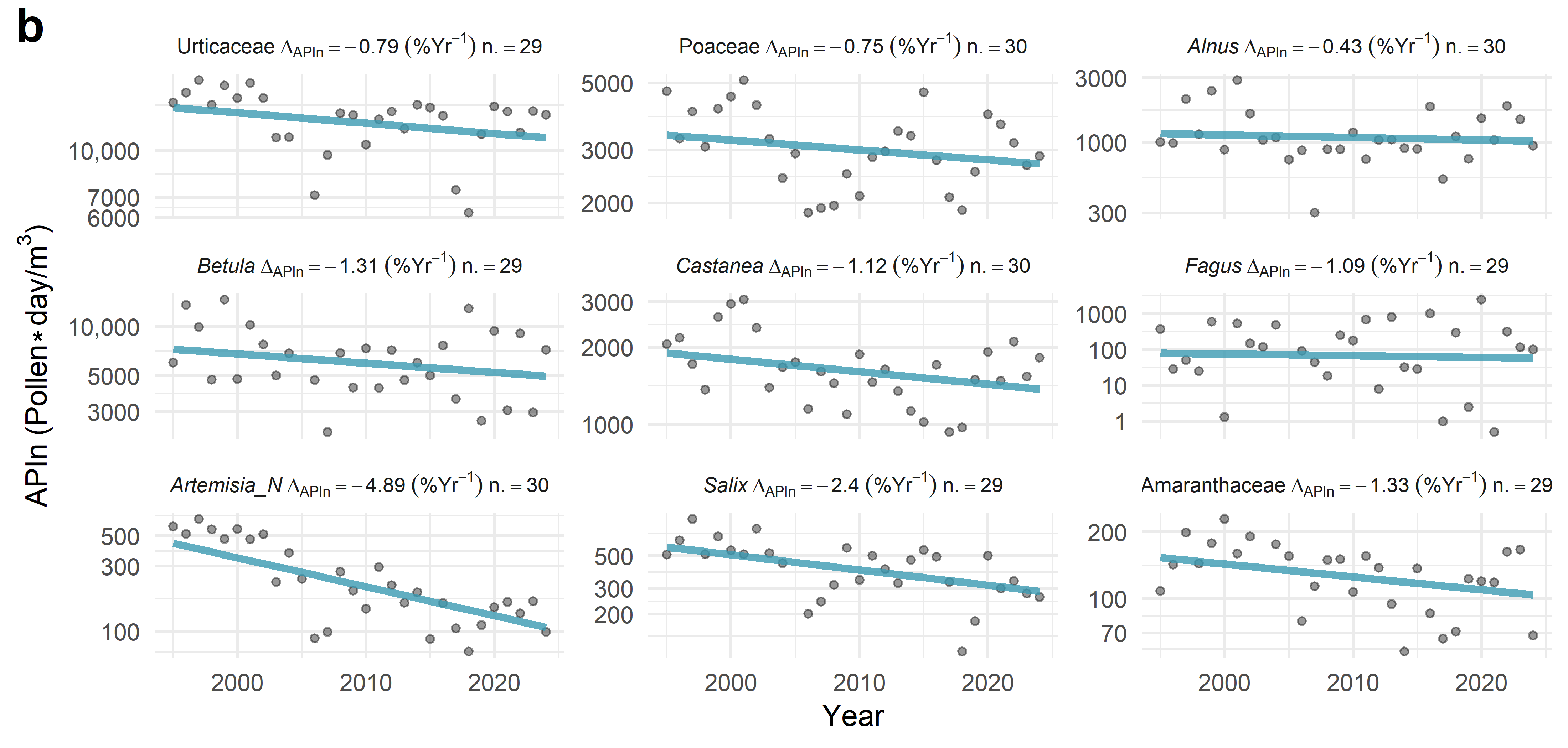
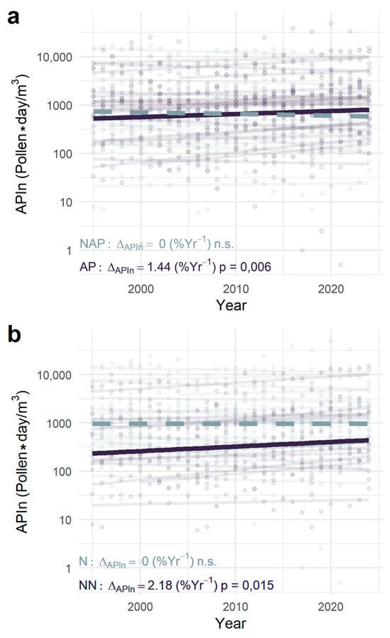
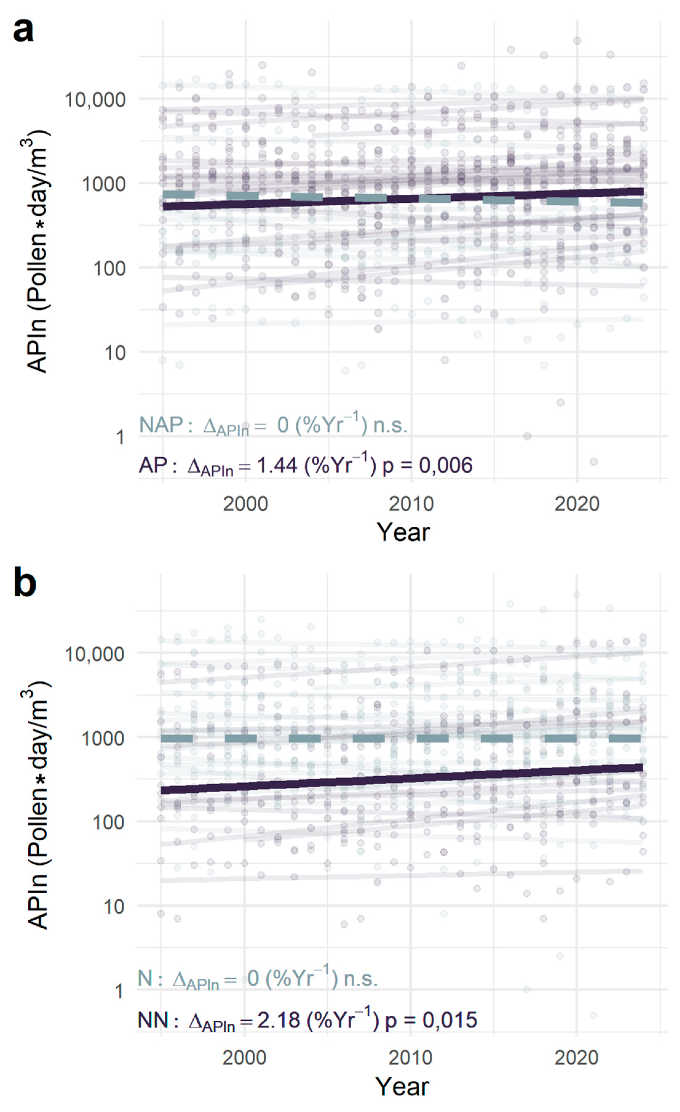

Disclaimer/Publisher’s Note: The statements, opinions and data contained in all publications are solely those of the individual author(s) and contributor(s) and not of MDPI and/or the editor(s). MDPI and/or the editor(s) disclaim responsibility for any injury to people or property resulting from any ideas, methods, instructions or products referred to in the content. |
© 2026 by the authors. Licensee MDPI, Basel, Switzerland. This article is an open access article distributed under the terms and conditions of the Creative Commons Attribution (CC BY) license.