


Abstract
Conductor icing threatens overhead transmission lines in mountainous North China, yet the relative contributions of different accretion pathways, including freezing rain, rime, and wet snow, remain poorly quantified. Five conductor icing events occurring in mountainous Beijing between February 2015 and March 2026 were analysed. In situ fibre-optic conductor icing observations were combined with meteorological fields from the fifth-generation European Centre for Medium-Range Weather Forecasts reanalysis (ERA5) and ERA5-Land, together with 30 m digital elevation model (DEM) data. A Makkonen-based accretion-flux framework was applied to distinguish between the freezing-rain/freezing-drizzle, in-cloud-rime, and wet-snow pathways. For the two events with complete hourly observations, the simulated numbers of observation sites with icing were positively correlated with observations (Spearman and for Cases 1 and 2, respectively), while the corresponding correlations for mean ice thickness were 0.394 and 0.749. Sensitivity experiments showed that Cases 2 and 4 were robustly rime-dominated, Case 3 was robustly wet-snow-dominated, and Case 5 was predominantly rime-dominated; Case 1 represented a near 0 °C mixed event in which the quantitative rime–wet-snow partition was parameter-sensitive. Freezing rain/freezing drizzle did not become the dominant pathway in any baseline or sensitivity configuration. The events shared a common sequence involving a 500 hPa short-wave trough, 850 hPa moisture transport, low-level convergence, orographic ascent, and the formation of supercooled low clouds at conductor elevation. Icing occurrence and larger ice thicknesses were more frequent at higher elevations, and the diagnosed rime accretion potential generally increased with elevation. These event-based results indicate that conductor icing assessments for mountainous North China should consider in-cloud rime, wet-snow adhesion, and terrain-modulated cloud exposure in addition to classical freezing-rain diagnostics, while broader regional generalisation requires a larger event sample.
1. Introduction
Atmospheric ice accretion is a major hazard to overhead transmission lines because the additional load can damage conductors, support structures, and fittings and contribute to galloping, flashover, and cascading outages [1,2,3,4]. The extensive power system damage caused by the freezing-rain and snowstorm disaster in southern China in early 2008 prompted sustained research on icing mechanisms, monitoring, and forecasting [1,4,5,6]. Much of that work has focused on freezing-rain-induced glaze in southern China, where icing is typically associated with persistent liquid precipitation and a classical “warm-above, cold-below” thermal structure [4,6,7,8]. By contrast, conductor icing in mountainous North China has received far less systematic attention, although damaging events continue to occur. Significant icing events have also been documented across northern China [9,10,11]. These include a widespread transmission line icing event in Shanxi Province in January 2022 that resulted in 31 line trips. Nevertheless, the dominant physical pathway, the formation mechanism, and the terrain controls of conductor icing in this region remain insufficiently quantified.
Atmospheric icing on conductors can arise from three principal hydrometeor sources: freezing rain or freezing drizzle, supercooled cloud or fog droplets, and wet snow [2,3,4,12]. These sources involve distinct thermodynamic structures, particle phases, and accretion processes. Classical freezing rain generally develops when solid precipitation melts in an elevated above-freezing layer and subsequently becomes supercooled within a subfreezing layer near the surface [13,14,15]. Rime forms when wind-transported supercooled cloud or fog droplets impinge on a subfreezing conductor and freeze; its growth is therefore governed by cloud liquid-water content, droplet size, wind-driven collision, temperature, and exposure duration [2,12,16,17,18]. Wet-snow accretion occurs near the melting point, when partially melted snowflakes contain sufficient liquid water to adhere to a conductor [12,18,19,20,21]. Consequently, conductor icing cannot be diagnosed reliably from surface precipitation or near-surface temperature alone; the vertical thermal structure, hydrometeor phase, and conductor-scale accretion conditions must be considered together.
The hydrometeor mass-flux formulation developed by Makkonen provides a common physical basis for describing these mechanisms [2,22,23]. In this formulation, the accretion rate depends on hydrometeor mass concentration, particle velocity relative to the structure, projected structural dimensions, and the collision, sticking, and freezing efficiencies [2,23,24]. Previous studies have used this framework to estimate ice loads from freezing precipitation [25,26], simulate or forecast in-cloud icing from clouds’ liquid water and wind [17,18,27,28], and model wet-snow accretion using snowfall supply and temperature-dependent adhesion [18,19,20,21]. These studies have established process-based methods for individual icing mechanisms. However, direct event-scale comparisons of freezing-precipitation, in-cloud-rime, and wet-snow accretion within a consistent flux framework—constrained by observed conductor icing—remain uncommon, particularly in North China.
Conductor icing also develops within a hierarchy of atmospheric and terrain-related processes. Synoptic disturbances and low-level moisture transport influence the development, depth, and phase of clouds and precipitation [4,5,6,7,8,15], while orographic ascent can modify saturation, supercooled liquid-water availability, and the spatial distribution of icing in mountainous terrain [4,16,18,28,29]. This terrain influence is particularly relevant to the distinction between classical freezing-precipitation icing and direct in-cloud icing. In the former, liquid precipitation is produced through melting in an elevated above-freezing layer before becoming supercooled near the surface, whereas in mountainous terrain, moist airflow can be lifted and cooled locally, allowing direct in-cloud icing without requiring a classical melting layer. Terrain-based transmission line studies have further shown that incorporating elevation and local landform information can improve icing prediction or spatial correction [4,30,31,32]. Nevertheless, terrain is often treated as an empirical predictor rather than as part of a process chain linking synoptic forcing, cloud microphysics and observed accretion. The roles of elevation in the occurrence, severity and pathway-specific potential of conductor icing therefore require further observational evaluation in mountainous North China.
Beijing, located in North China, provides a suitable setting for this investigation because operational conductor icing observations are available for multiple events. This study analyses five documented events with clearly observed conductor icing between February 2015 and March 2026 using conductor icing records, the fifth-generation European Centre for Medium-Range Weather Forecasts (ECMWF) reanalysis (ERA5) and ERA5-Land, and digital elevation data. The objectives are to (1) characterise the temporal evolution and synoptic-to-local atmospheric environments of two events with complete hourly icing records; (2) diagnose and compare the freezing-rain/freezing-drizzle, in-cloud-rime and wet-snow accretion pathways for all five events within a unified accretion-flux framework; and (3) quantify the relationship of elevation to icing occurrence, ice thickness and pathway-specific accretion potential. The analysis links large-scale circulation, low-level hydrometeor conditions, conductor-scale accretion and terrain-dependent spatial variability within a common process-oriented framework. The two hourly observed events are additionally used to validate the simulated icing evolution, and sensitivity experiments are used to assess the robustness of the pathway diagnosis for all five events. The cases were selected for process diagnosis rather than through random sampling and are not intended to represent a statistically complete regional icing climatology.
2. Materials and Methods
2.1. Study Area and Icing Observations
The study domain covers Beijing, China, with emphasis on its mountainous areas. Terrain elevation was obtained from the National Aeronautics and Space Administration Shuttle Radar Topography Mission 1 arc-second Digital Elevation Model (SRTM1 DEM), distributed by the United States Geological Survey (USGS) at an approximate spatial resolution of 30 m [33]. Elevation increases from approximately 50 m on the southeastern plain to low and medium mountains and reaches 2303 m at Dongling Mountain in Beijing (Figure 1a). The region includes plains, foothills, valleys, slopes, and ridges.
Figure 1.
(a) Terrain of Beijing derived from the SRTM1 DEM, showing the municipal boundary, the generalized icing observation area, and the Beijing radiosonde station (WMO 54511; 39.93° N, 116.28° E). The red rectangle denotes the generalized icing observation area. (b) Example FBG-based conductor icing monitoring system adapted from Figure 4 in the original study by Zhang et al. [34] under the Creative Commons Attribution 4.0 International License (CC BY 4.0); the source image was resized, placed in the composite, and relabelled as panel (b). Abbreviations: SRTM1, Shuttle Radar Topography Mission 1 arc-second; DEM, digital elevation model; WMO, World Meteorological Organization; FBG, fibre Bragg grating; OPGW, optical fibre composite overhead ground wire.
In situ conductor icing observations were obtained primarily through distributed fibre-optic sensing; Figure 1b illustrates an example fibre Bragg grating (FBG)-based icing-monitoring system adapted from Zhang et al. [34]. Optical fibre composite overhead ground wire (OPGW)- and FBG-based systems can retrieve icing-related strain, vibration, or temperature information from multiple locations along the sensing fibre, thereby enabling broader observational coverage across mountainous terrain than conventional single-point measurements [35,36,37,38]. The monitoring records provide icing occurrence, duration, affected locations, and equivalent ice thickness and were used to analyse event evolution and elevation-dependent spatial variability.
2.2. Icing Events and Observational Data
Five events with well-documented conductor icing were selected from the available Beijing operational record from 2015 through March 2026 (Table 1; Figure 1a): 25 February–6 March 2026 (Case 1), 12–16 December 2023 (Case 2), 19–22 November 2016 (Case 3), 20–26 November 2015 (Case 4), and 20–22 February 2015 (Case 5). For all other reported icing observations in the available record, the maximum reported ice thickness was below 1 mm. The selected events cover a range of near-surface temperature and precipitation conditions, and their dominant accretion pathways are diagnosed from the atmospheric and hydrometeor conditions in Section 3. Because the selection targeted cases with clearly measurable icing rather than random or exhaustive sampling, the five cases support process diagnosis but should not be interpreted as a statistically complete sample of all icing events in mountainous Beijing.
Table 1.
Conductor icing events and observational records used in this study.
Complete hourly fibre-optic records were available for Cases 1 and 2, allowing reconstruction of the co-evolution of equivalent ice thickness, temporal changes in the number of observation sites with icing, meteorological conditions, and pathway-specific accretion fluxes. Case 3 was documented by daily reports containing affected locations and maximum ice thickness. Cases 4 and 5 pre-dated the operational fibre-optic records used here and were identified from retrospective manual-observation summaries containing icing dates and affected locations. Accordingly, quantitative model–observation validation was restricted to Cases 1 and 2. For Cases 3–5, the sensitivity experiments were used only to evaluate the robustness of pathway flux fractions and dominant-pathway classification.
The hourly records for Cases 1 and 2 were quality controlled before analysis. A detection was classified as effective icing only when the equivalent ice thickness exceeded 0.5 mm and remained above this threshold continuously for more than 3 h. Values exceeding 100 mm were treated as instrumental anomalies and removed. Analyses of Cases 3–5 used only the icing information explicitly reported in the corresponding records together with the collocated reanalysis fields.
2.3. Meteorological and Terrain Data
Five data categories were integrated (Table 2). Hourly ERA5 reanalysis data at 0.25° resolution were used for synoptic circulation, vertical thermodynamic structure, and hydrometeor diagnosis [39]. The pressure-level variables were geopotential, air temperature, relative humidity, horizontal wind, vertical velocity, specific cloud liquid water content (CLWC), specific rain water content (CRWC), and specific snow water content (CSWC). Because this resolution is much coarser than individual ridges, valleys and local-scale cloud structures, the interpolated CLWC, CRWC, and CSWC fields are treated as indicators of the regional icing environment rather than direct measurements of local-scale cloud microphysics. The sensitivity to unresolved spatial variability is evaluated separately in Section 2.4.5.
Table 2.
Data inventory.
Hourly ERA5-Land data at 0.1° resolution were used for the near-surface environment throughout 2015–2026 [40]. The variables were 2 m air temperature, 2 m dew-point temperature, 10 m zonal and meridional wind, surface pressure, and total precipitation. Wind speed was calculated from the two horizontal components. Relative humidity was derived from air and dew-point temperatures, and wet-bulb temperature was calculated from air temperature, relative humidity, and surface pressure.
Routine upper-air observations from the Beijing radiosonde station (World Meteorological Organization [WMO] station number 54511; 39.93° N, 116.28° E; Figure 1a) were obtained from the University of Wyoming Atmospheric Science Radiosonde Archive and used as an independent evaluation of the ERA5 vertical thermodynamic structure. The archive provides routine soundings for this station at the standard 00:00 and 12:00 Coordinated Universal Time (UTC) launch times, corresponding to 08:00 and 20:00 Beijing time, respectively, giving a routine temporal resolution of 12 h. All available soundings whose launch times fell within the five event windows were included in the analysis.
The SRTM1 DEM was used to assign elevation to each observation site or manually reported icing location, delineate the principal terrain features shown in Figure 1, and define the elevation bands used in the spatial analysis [33].
2.4. Location-Based Accretion Rate Framework
Three hydrometeor pathways were diagnosed separately: freezing rain or freezing drizzle, supercooled cloud droplets, and wet snow. These produce glaze, rime, and wet-snow accretion, respectively, and differ in particle size, relative velocity, collision behaviour, adhesion, and freezing process [2,3,19,20,21].
Following the Makkonen framework and International Organization for Standardization (ISO) standard 12494 [2,22,25], the icing mass growth rate per unit conductor length was calculated as
where is ice mass per unit conductor length; is volumetric hydrometeor mass concentration; is particle velocity relative to the conductor; is the projected conductor width; and , , and are the collision, sticking, and freezing/accretion efficiencies. A bare conductor diameter of m was adopted. In the baseline integration, the projected collection width was updated as retained equivalent ice accumulated; keeping the projected width fixed at was tested as a sensitivity experiment.
For pathway , at analysis location (an observation site or a reported icing location, as applicable) and hour , the per-unit-length accretion rate and its cumulative value were
where s. Thus, has units of kg m−1 s−1 and has units of kg m−1. The pathway fractions used below refer to the time-integrated gross accreted masses per unit conductor length. They should therefore be interpreted as diagnostic pathway contributions rather than the measured composition of the final ice deposit.
In the baseline (H00) forcing, ERA5 pressure-level variables were sampled from the nearest 0.25° grid point to each analysis location and then vertically matched using geopotential height; pressure levels below the model surface were excluded. ERA5-Land variables were bilinearly interpolated to the same analysis locations. The hydrometeor and air-density fields used in all pathway calculations were evaluated at the adopted 30 m conductor height above local ground. Hydrometeor mixing ratio was converted to volumetric content using , where , is air pressure, is the dry-air gas constant, and is virtual temperature. ERA5 pressure-level specific humidity was used to calculate and during forcing construction. The resulting 30 m volumetric contents were used consistently for the rime, wet-snow and glaze pathways.
Because ERA5-Land provides wind at 10 m whereas the conductors are suspended above the near-surface reference level, the horizontal wind was extrapolated to conductor height before being used in the relative-velocity and collision-efficiency calculations. A power-law wind profile was applied:
where is the estimated conductor-height wind speed and is the conductor height above local ground. A representative value of m was adopted. The wind-shear exponent was allowed to decrease with increasing 10 m wind speed:
These values were derived from one year of 10–70 m wind-mast observations at a mountainous wind-mast observation site in Shandong, northern China, where the corresponding shear exponents were 0.336, 0.275, and 0.202 for 10 m wind speed classes of <2, 2–6, and 6–12 m s−1, respectively [41]. The last branch of Equation (5) is written as m s−1 to provide a complete implementation, but use above 12 m s−1 would be an extrapolation beyond the source observations. The maximum unperturbed 10 m wind speed across the five baseline event forcings was 6.42 m s−1, so this out-of-range extrapolation was not invoked in the baseline analyses. The shear at that wind-mast observation site was larger than that over the nearby plain and offshore surface because complex terrain and greater surface roughness exert stronger frictional control on the lowest layer, suppressing 10 m wind more strongly than the wind aloft. At the adopted 30 m conductor height, Equation (4) corresponds to multipliers of approximately 1.45, 1.35, and 1.25 for the three wind speed classes. All occurrences of horizontal wind in the pathway equations below refer to unless otherwise stated. The conductor height and wind-extrapolation formulation were subsequently varied in the sensitivity experiments.
For event-scale time series, the hourly per-unit-length accretion rate was averaged over valid analysis locations:
For inter-event comparison, the time-integrated accreted masses per unit length at each analysis location were averaged over the locations associated with each event. For the elevation analysis, all observation sites with valid forcing data were grouped by DEM-derived elevation, and the mean time-integrated accretion potential in elevation band was calculated across all observation sites in that band. These band means include records with and without observed icing and therefore characterise the potential accretion environment within each elevation band.
2.4.1. Freezing-Rain and Freezing-Drizzle Pathway
Classical freezing rain requires falling ice particles to melt partially or completely in an elevated above-freezing layer and then enter a subfreezing layer near the conductor [13,14,42]. The temperature profile was evaluated at each analysis location. At each analysis location and hour, conditions were classified as a classical freezing-rain environment when (i) a continuous above-freezing layer occurred aloft, detected on the pressure levels at and above 850 hPa; (ii) subfreezing air occurred immediately below and above it, producing a cold–warm–cold structure; (iii) the conductor-height or near-surface temperature was no higher than 0 °C; and (iv) the interpolated warm layer was at least 200 m thick and its peak temperature reached at least 1 °C. The lower and upper 0 °C crossings were linearly interpolated in geometric height, and warm-layer thickness was calculated as . The 200 m and 1 °C thresholds were study-specific conservative filters used to reject shallow numerical fluctuations near 0 °C, not universal precipitation-type boundaries. Both thresholds were varied in the sensitivity experiments.
Freezing drizzle can form without an elevated melting layer through collision–coalescence in a shallow supercooled liquid cloud [43]. It was considered possible when CRWC at conductor height was measurable and both the conductor environment and liquid-cloud layer were subfreezing. Concurrent CRWC and CLWC were compared to distinguish a rain/drizzle contribution from a cloud-droplet-dominated rime environment. Thus, the absence of an elevated melting layer did not by itself exclude glaze accretion: CRWC-resolved supercooled liquid precipitation under subfreezing conditions was still included in the glaze pathway. Very local or short-lived liquid precipitation not represented in the ERA5 CRWC field may nevertheless remain unresolved.
The relative velocity of liquid precipitation combined horizontal wind and gravitational fall speed:
where m s−1 represents a 1 mm liquid drop [44,45,46]. The collision and sticking efficiencies were set to . Rain-sized drops have sufficient inertia that streamline deflection around a conductor is weak, and liquid drops that strike a subfreezing, wetted, or ice-covered surface are assumed to spread, adhere, or freeze rather than rebound [2,25,26].
Glaze generally develops under wet-growth conditions; therefore, the physical freezing efficiency can be less than unity because part of the incident water remains liquid and runs off [2,25]. Conductor-surface temperature, heat-transfer coefficients, and runoff were unavailable, so was used to represent the limiting maximum glaze-accretion potential. The resulting glaze flux is an upper bound and not an absolute glaze-growth rate. Sensitivity experiments additionally used , 0.4, 0.6, and 0.8 and raindrop terminal fall speeds from 2.0 to 7.0 m s−1.
The time-integrated gross glaze accretion was
where is the set of hours at analysis location satisfying the classical freezing-rain or freezing-drizzle criteria.
2.4.2. In-Cloud Rime Pathway
At each analysis location and hour, conditions were assigned to the rime pathway when (i) near-surface air temperature was below 0 °C and (ii) the 30 m volumetric CLWC was greater than zero [2,3,16,17]. Relative humidity was retained as a descriptive environmental variable but was not imposed as an additional pathway threshold. Cloud-droplet terminal fall speed was neglected relative to horizontal wind, so the relative velocity was approximated as .
Because small cloud droplets can follow streamlines around a cylinder, the collision efficiency was calculated using the Finstad–Makkonen parameterisation [2,47]:
Here, kg m−3, Pa s, is conductor diameter, is median volume diameter (MVD), and was obtained from the ERA5 fields, whereas was derived from ERA5-Land 10 m wind using Equations (4) and (5).
Because event-specific droplet size spectra were unavailable, a representative MVD of 25 μm was adopted. Typical cloud droplets are of order 10 μm in radius, corresponding to diameters near 20 μm [48]. Because MVD is weighted by liquid-water volume and therefore gives greater importance to the larger droplets in a size distribution than a number-weighted mean diameter, a value slightly above the characteristic cloud-droplet diameter was selected as the baseline. Mountain wire-icing observations also show a broad fog droplet range of approximately 2–50 μm [12]. Sensitivity experiments using MVDs of 10, 15, 20, and 30 μm were conducted to assess this uncertainty.
The calculated Finstad–Makkonen efficiency was constrained only to its physical range, . As a model-form sensitivity test, fixed rime collision efficiencies of 0.05, 0.12, 0.20, 0.30, 0.40, and 0.60 were also evaluated [23,49].
The sticking efficiency was set to because supercooled droplets that collide with a subfreezing conductor or existing rime deposit are assumed to remain on the surface. The freezing efficiency was set to because rime is treated as dry growth, for which the small incident droplets freeze completely and runoff is negligible [2]. The time-integrated gross rime accretion was
where is the set of hours at analysis location satisfying the rime criteria.
2.4.3. Wet-Snow Pathway
Wet-snow accretion was diagnosed in the narrow thermodynamic interval in which snow particles are partly melted and sufficiently adhesive to remain on a conductor [19,20,21]. Wet-bulb temperature was used because it represents the combined effects of air temperature and humidity on melting and surface liquid-water availability. At each analysis location and hour, wet-snow conditions were identified when (i) °C and (ii) volumetric CSWC at conductor height was greater than zero. This operational interval identifies snow close to melting while excluding colder dry snow and predominantly liquid precipitation. The upper wet-bulb temperature limit was varied between 0.5 and 2.0 °C in the sensitivity experiments.
The collision efficiency was set to because wet snowflakes and aggregates are much larger than cloud droplets and have sufficient inertia to limit streamline avoidance around a conductor [2,19,20,21]. A representative terminal fall speed of m s−1 was used [21], giving
Wet-snow sticking is incomplete because some flakes rebound or detach after impact. A commonly used first-order approximation for a cylindrical collector is , with in m s−1 [2,20,22]. In this study, the approximation was applied to the total relative impact speed:
An alternative dependence was tested as a sensitivity experiment. Snow-particle fall speed was also varied from 1.0 to 2.8 m s−1.
The freezing/accretion efficiency was set to : once a partly melted particle is retained, its full water-equivalent mass is counted as accumulated, without imposing a separate instantaneous-freezing limitation [2,19,20,21]. Values of 0.2, 0.4, 0.6, and 0.8 were additionally tested to represent uncertainty in wet-snow retention.
The time-integrated gross wet-snow accretion was
where is the set of hours at analysis location satisfying the wet-snow criteria.
2.4.4. Event Classification
For pathway , the event-scale percentage contribution was calculated as
where .
The pathway percentages are diagnostic gross-accretion fractions rather than exact fractions of the observed final ice mass. The pathway with the largest time-integrated gross accreted mass per unit length was identified as the baseline dominant pathway, and the classification was interpreted by examining the temporal consistency between diagnosed accretion and observed icing where hourly observations were available. The sensitivity experiments were then used to determine whether the dominant classification was robust. Events for which plausible parameter settings caused shifts in the dominant accretion pathway were described as mixed or parameter-sensitive rather than assigned categorically to a single mechanism.
The baseline efficiency factors, representative fall speeds, and relative velocities are summarised in Table 3.
Table 3.
Efficiency factors, representative fall speeds, and relative velocities used in the baseline accretion-flux calculations.
2.4.5. Validation and Sensitivity Analysis
To evaluate whether the diagnosed accretion fluxes reproduced the observed icing evolution rather than merely identifying favourable atmospheric conditions, the pathway-specific fluxes were integrated forward to obtain retained ice mass per unit conductor length and then converted to equivalent radial ice thickness. Under the cylindrical-equivalent assumption used in the code, the radial thickness was , where is the retained mass of pathway per unit conductor length and is its bulk density. The projected collection width at hourly step was the equivalent outer diameter from the preceding step, . The bulk density of accreted ice varies substantially with icing type. ISO 12494:2017 gives a representative density of 900 kg m−3 for glaze, a range of 300–600 kg m−3 for wet snow, and ranges of 200–600 and 600–900 kg m−3 for soft and hard rime, respectively [22]. Based on these ranges, baseline densities of 900, 500, and 300 kg m−3 were adopted for glaze, rime, and wet snow, respectively. To quantify uncertainty in the conversion from retained ice mass to equivalent radial thickness, one-factor-at-a-time density sensitivity experiments were additionally conducted using 700 and 800 kg m−3 for glaze, 300 and 700 kg m−3 for rime, and 450 and 600 kg m−3 for wet snow. Melting and sublimation losses were represented using field-derived relations from Savadjiev and Farzaneh [50]. A constant loss rate of 0.007 kg m−1 h−1 was applied at air temperatures ≤ −0.4 °C; at higher temperatures, the loss rate was kg m−1 h−1, where is air temperature in °C. The latter empirical relation represents the combined mass decrease associated with melting and mechanical breakage. At each hourly step, pathway-specific accretion was added first, and the applicable loss was then subtracted, limited by the available retained ice mass. No additional independent wind-shedding term was imposed.
Validation was performed for Cases 1 and 2, for which complete hourly ice-thickness records were available. Observed and simulated numbers of observation sites with icing and mean equivalent ice thickness were compared using Spearman’s rank correlation coefficient, , where and denote the observed and simulated values, respectively, at hourly time step , for either the number of observation sites with icing or mean equivalent ice thickness over the full hourly comparison series. Spearman correlation was selected because it is a rank-based measure of monotonic association that does not require a linear relationship or normality and is suitable for series containing repeated zero values [51]. To quantify the magnitude accuracy of simulated mean equivalent radial ice thickness, mean absolute error (MAE), root mean square error (RMSE), and mean bias were additionally calculated over the observed icing interval as , , and , where is the number of hourly samples within the magnitude-error evaluation interval. Negative bias indicates systematic underprediction. Cases 3–5 were not assigned quantitative validation statistics because their observational records lack complete hourly ice-thickness series.
The complete baseline configuration and sensitivity-experiment design are summarised in Supplementary Table S1. The one-factor-at-a-time deterministic sensitivity experiments comprised 52 variants per case and were organised into three groups: I, microphysics and efficiency (36 variants); II, forcing and conductor scale (7 variants); and III, geometry and phase diagnosis (9 variants). A fourth group, IV, evaluated ERA5 resolution and spatial representativeness through the 63 spatial configurations described below. The same grouping is used below to identify the source of the sensitivity in the simulated temporal evolution and diagnosed accretion pathways.
To assess uncertainty associated with the empirical loss treatment, Cases 1 and 2 were additionally tested using loss rate multipliers of 0.5, 1.5, 2.0, and 3.0 relative to the baseline. Because this sensitivity test targets post-accretion ice loss rather than the accretion pathways themselves, it was conducted separately from the 116-run pathway classification experiment suite. Accordingly, varying the loss rate affects retained-ice validation but does not alter the gross pathway fractions or dominant-pathway classification, which are determined from gross accretion before ice loss.
The ERA5 spatial representativeness experiments comprised three sampling controls and 60 stochastic members, giving 63 configurations per case. H00 was the baseline and used nearest-neighbour horizontal sampling of the original 0.25° ERA5 pressure-level fields, H01 directly bilinearly interpolated those fields to the analysis locations, and H02 first interpolated the fields to a 3 km Lambert grid and then to the analysis locations without random perturbation. H02 was therefore used only as an interpolation control rather than as a higher-resolution reconstruction. The 60 stochastic members were generated by perturbing six forcing groups—temperature, specific humidity, horizontal wind, liquid hydrometeors (CLWC + CRWC), snow water content (CSWC), and all variables jointly—using two perturbation amplitudes ( and ) and five random seeds for each amplitude. For the specific-humidity perturbation, the starting specific humidity at conductor height was diagnosed from co-located temperature, relative humidity, and pressure before perturbation, and relative humidity was recalculated afterwards.
The perturbations were constructed as spatially and temporally correlated random fields on the 3 km grid to represent unresolved sub-grid variability within the coarse ERA5 forcing. Temperature and wind were perturbed additively, whereas humidity and hydrometeors used multiplicative perturbations; liquid hydrometeors and snow water content were additionally constrained to preserve the sampled water amount within each group of analysis locations in an original ERA5 grid cell. In the combined-forcing members, separate random fields were generated for temperature, specific humidity, the two wind components, liquid hydrometeors, and snow water content; no cross-variable covariance was imposed, although CLWC and CRWC shared the same liquid-hydrometeor field. Wet-bulb temperature and all derived icing variables were then recalculated before reintegrating the icing model from zero retained mass. The amplitude factors and therefore represent lower- and higher-amplitude perturbation settings rather than uniform ±50% and ±100% changes. Full perturbation equations and parameter settings are provided in the Supplementary Materials.
ERA5 vertical atmospheric profiles were independently evaluated against routine radiosonde observations from Beijing station WMO 54511 for all five events. The station provides routine soundings at 00 and 12 UTC, and all soundings falling within the event windows were included, yielding 54 collocated profiles. Radiosonde observations were interpolated in log-pressure to the corresponding ERA5 pressure levels, while ERA5 temperature, relative humidity, and horizontal wind components were bilinearly interpolated to the station location at the sounding times. Comparisons were performed over 1000–500 hPa using bias, mean absolute error (MAE), root mean square error (RMSE), and Pearson correlation coefficient. Because WMO 54511 is located on the Beijing plain, this evaluation represents the regional vertical atmospheric structure rather than local-scale mountain-cloud conditions. The analyses were performed using Python 3.12.
2.4.6. Elevation Association Analysis
Elevation dependence was analysed for Cases 1–3 using 100 m elevation bands. For each case, the observed icing fraction within each band was calculated as the number of records with icing from observation sites divided by the total number of monitored records from observation sites, with uncertainties expressed as Wilson 95% binomial confidence intervals [52].
To examine whether the elevation association persisted after accounting for meteorological conditions, we fitted a multivariable logistic regression model to the binary icing status recorded at each observation site during each event [52]. Predictors included elevation (per 100 m), 2 m air temperature, conductor-height wind speed, CLWC, and case. Cluster-robust standard errors were used to account for repeated records from the same observation site across different events. Results are reported as odds ratios with 95% confidence intervals. Because the locations of observation sites and the meteorological conditions are spatially correlated, the fitted effects are interpreted as conditional associations rather than causal relationships.
3. Results
3.1. Icing Evolution of Two Representative Events and Its Relation to Meteorological Conditions and Accretion Fluxes
Figure 2 presents the observed icing evolution, meteorological conditions, and pathway-specific accretion fluxes from the baseline experiment for Cases 1 and 2. Figure 3 compares the observed and simulated hourly numbers of observation sites with icing and mean equivalent radial ice thickness under the baseline configuration. Figure 4 and Figure 5 then summarise all experimental runs using a common grouping: Baseline; I, microphysics and efficiency; II, forcing and conductor scale; III, geometry and phase diagnosis; and IV, ERA5 resolution and spatial representativeness. Figure 4 presents the observation–simulation Spearman correlations, whereas Figure 5 presents the corresponding gross accretion pathway fractions.
Figure 2.
Hourly evolution during Case 1 (left column) and Case 2 (right column), including (a,b) observed mean ice thickness and number of observation sites with icing, (c,d) near-surface air temperature and relative humidity, with the dashed line marking 0 °C, (e,f) 10 m wind speed and precipitation, and (g,h) hydrometeor contents and diagnosed rime, wet-snow and freezing-rain/freezing-drizzle accretion fluxes from the baseline experiment. Times are in Beijing time.
Figure 3.
Comparison of observed and baseline-simulated icing evolution for Cases 1 and 2, including (a) the number of observation sites with icing for Case 1, (b) mean equivalent radial ice thickness for Case 1, (c) the number of observation sites with icing for Case 2, and (d) mean equivalent radial ice thickness for Case 2. The corresponding Spearman correlation coefficients are and 0.394 for Case 1 and and 0.749 for Case 2. For mean equivalent radial ice thickness, the MAE, RMSE, and mean bias are 2.002, 2.535, and −1.643 mm for Case 1 and 2.254, 2.317, and −2.215 mm for Case 2, respectively.
Figure 4.
Observation–simulation Spearman correlations across all experiments for Cases 1 and 2. Panels (a,b) show Case 1 correlations for the number of observation sites with icing and mean equivalent radial ice thickness, respectively, and panels (c,d) show the corresponding results for Case 2. The star denotes the baseline experiment. Circles, squares, diamonds, and triangles denote groups I–IV, respectively: I, microphysics and efficiency; II, forcing and conductor scale; III, geometry and phase diagnosis; and IV, ERA5 resolution and spatial representativeness. Open symbols plotted at NA indicate configurations for which Spearman is undefined because the simulated evaluation series is constant or contains no effective icing above the evaluation threshold.
Figure 5.
Gross accretion pathway fractions across all experiments: (a) freezing-rain/freezing-drizzle glaze for Case 1; (b) freezing-rain/freezing-drizzle glaze for Case 2; (c) rime for Case 1; (d) rime for Case 2; (e) wet snow for Case 1; and (f) wet snow for Case 2. The star denotes the baseline experiment, and circles, squares, diamonds, and triangles denote groups I–IV as defined in Figure 4. Each percentage is the time-integrated gross accreted mass per unit length of the indicated pathway divided by the sum over the three pathways. NA denotes a configuration with zero total gross accretion, for which pathway fractions are undefined.
Case 1 exhibited a complex, intermittent evolution comprising three distinct icing sub-processes (Figure 2a).
- (1)
- The first sub-process of Case 1 occurred from midday on 25 February to the early morning of 26 February, when weak icing was observed at only a few observation sites (Figure 2a). Cloud liquid water and the rime accretion flux increased before and during the observed icing, while wet-snow accretion also contributed, and the freezing-rain glaze flux remained much weaker (Figure 2g). The simultaneous occurrence of rime and wet-snow fluxes indicated a mixed near 0 °C accretion environment rather than a clearly separated single-pathway episode. Subsequent warming, drying, and weakening of the accretion fluxes led to the rapid disappearance of this limited ice accumulation.
- (2)
- The second sub-process was the longest and most intense. Rapid ice growth occurred from approximately 08:00 Beijing time on 27 February to 12:00 on 28 February and coincided with enhanced cloud-water and wet-snow accretion conditions (Figure 2a,g). Snowfall and an associated wet-snow flux occurred before and during this rapid growth period. From 12:00 on 28 February to approximately 18:00 on 2 March, the event entered a maintenance stage. Mean ice thickness remained near 3–4 mm, and recurrent high relative humidity favoured ice persistence. A further, weaker intensification around 3 March coincided with another increase in cloud-water accretion. After midday on 3 March, pronounced warming and drying terminated further accretion and led to rapid melting.
- (3)
- The third sub-process redeveloped on 4 March, when subfreezing temperatures, increasing humidity, and renewed cloud-water supply produced a short rime accretion episode with relatively small mean thickness. The observed ice thickness then decreased rapidly despite air temperatures remaining below 0 °C, ruling out melting as the principal cause. The simultaneous decline in relative humidity and cloud-water supply, together with wind exposure, is consistent with sublimation and/or mechanical shedding, while some observations also fell below the effective icing threshold.
Under the baseline configuration, the event-integrated gross accretion fractions for Case 1 were 23.9% rime, 69.5% wet snow, and 6.6% glaze. However, the relative dominance of rime and wet snow changed under several sensitivity configurations. Case 1 is therefore interpreted as a near 0 °C mixed and parameter-sensitive event rather than a robust single-pathway case.
Case 2 comprised a continuous sequence of rapid growth, spatial expansion, and overall decay (Figure 2b). Stable subfreezing temperatures, high humidity, and rime accretion conditions were already present early in the event, but effective icing appeared slightly later than the strengthening of the accretion flux (Figure 2d,h). After icing formed, the mean thickness increased rapidly and then remained essentially stable, while the number of observation sites with icing increased continuously, indicating that this stage was dominated by spatial expansion rather than by further growth at individual observation sites. Several later precipitation episodes were not accompanied by a further increase in mean ice thickness, and the spatial coverage of icing increased only slightly once widespread icing had been established. This lack of a synchronous ice response indicates that surface precipitation alone is not a reliable indicator of effective conductor accretion. During the decay stage, the temperature continued to fall, but relative humidity and cloud-water supply decreased markedly. Wind speed strengthened, the rime flux approached zero, and the count consequently decreased rapidly. In the absence of warming, this decay is more consistent with interruption of the cloud-water supply, sublimation, and/or wind-induced mechanical shedding than with melting. In the baseline experiment, the gross accretion in Case 2 was entirely attributed to rime, and the rime-dominated classification was retained throughout all experimental runs with defined pathway fractions.
Overall, icing growth in both events was jointly controlled by the thermal and humidity environment, hydrometeor supply, and pathway-specific accretion fluxes, with no simple one-to-one correspondence to surface precipitation. Case 1 occurred under near 0 °C conditions, with repeated low-cloud development and a substantial wet-snow contribution, and therefore evolved as a multi-round mixed icing process. Case 2 remained under persistently subfreezing conditions, high humidity, and sustained cloud-water supply and developed as a single rime-dominated process with rapid spatial expansion. Its peak count was substantially larger than that in Case 1. In addition to the broader and more persistent rime accretion environment, the substantially lower temperature in Case 2 likely suppressed melting and promoted more widespread ice persistence.
The direct observation–simulation comparison is shown in Figure 3. For Case 1, the Spearman correlation between the observed and simulated hourly numbers of observation sites with icing was 0.716, while that for mean equivalent radial ice thickness was 0.394. For Case 2, the corresponding correlations were 0.928 and 0.749, respectively. For the magnitude error metrics, evaluated from the first positive observed hourly mean thickness through the first zero-valued hour after the final positive observation, the MAE, RMSE, and mean bias were 2.002, 2.535, and −1.643 mm for Case 1 and 2.254, 2.317, and −2.215 mm for Case 2, respectively. These negative mean biases indicate systematic underestimation of mean ice thickness in both cases. One plausible contributor is the coarse spatial resolution of the ERA5 pressure-level fields, which can smooth ridge- and valley-scale maxima in cloud liquid water and snow water contents and thereby underrepresent local hydrometeor supply. The spatial representativeness experiments further indicate that the simulated icing evolution is sensitive to unresolved meteorological and hydrometeor variability (Figure 4, Group IV). However, because direct observations of cloud liquid water and snow water contents were unavailable, it was not possible to determine whether ERA5 systematically underestimated the hydrometeor content during these events.
Across the baseline and the four tested loss rate multipliers (0.5×, 1.5×, 2.0×, and 3.0×), the dominant pathway remained wet snow for Case 1 and rime for Case 2. For Case 1, Spearman ρ ranged from 0.695 to 0.716 for the number of observation sites with icing and from 0.370 to 0.394 for mean thickness, while MAE and RMSE ranged from 1.997 to 2.018 mm and from 2.528 to 2.573 mm, respectively. For Case 2, the corresponding correlation ranges were 0.909–0.942 and 0.535–0.755, while MAE and RMSE ranged from 2.254 to 2.296 mm and from 2.317 to 2.370 mm, respectively. The relatively high correlations, especially for Case 2, indicate that the simulations capture aspects of the timing and relative changes in icing occurrence. However, the MAE, RMSE, and negative mean biases show that absolute retained ice thickness is not reproduced accurately and is systematically underestimated. The limited changes in MAE and RMSE across the tested loss-rate range further suggest that the magnitude error cannot be explained by the empirical loss formulation alone. Complete values, including mean bias, are reported in Supplementary Table S4.
Figure 4 shows that the observation–simulation correspondence is not confined to the baseline parameter set. For Case 1, the deterministic groups I–III yielded positive correlations for the number of observation sites with icing, with ρ ranges of 0.377–0.813, 0.305–0.766, and 0.365–0.767, respectively; the corresponding mean thickness correlations were 0.091–0.755, 0.300–0.412, and 0.289–0.402. Group IV showed the widest spread, with ρ ranging from −0.083 to 0.800 for the count and from −0.192 to 0.708 for mean thickness, with only a few negative members. Case 2 was substantially more stable: all defined correlations remained high, with ρ for the number of observation sites with icing ranging from 0.878 to 0.954 and mean thickness ρ ranging from 0.489 to 0.767 across groups I–IV. Two experiments using the smallest MVD values produced undefined correlations because the simulated evaluation series was constant or contained no effective icing above the evaluation threshold. The wider correlation ranges in Case 1 indicate greater sensitivity of the simulated temporal correspondence to the tested configurations.
Figure 5 shows how the relative contributions of the three icing pathways change across the sensitivity experiments. In Case 1, group I produces the largest variation between rime and wet snow: the rime fraction ranges from 0 to 69.58%, while the wet-snow fraction ranges from 27.79 to 91.36%. The ranges are narrower in groups II–IV, although both rime and wet snow remain substantial in several configurations. Glaze remains small in every group, with a maximum fraction of 14.82%, and never becomes dominant. The resulting change in the dominant pathway between wet snow and rime therefore supports the interpretation of Case 1 as a mixed, parameter-sensitive event. By contrast, Case 2 remains 100% rime in every configuration with non-zero total accretion.
An independent comparison with Beijing radiosonde observations further evaluated the ERA5 atmospheric fields used in the analysis (Supplementary Figure S8). Across the 54 collocated profiles over 1000–500 hPa, temperature had a bias of −0.35 °C, MAE of 0.78 °C, RMSE of 1.06 °C, and Pearson correlation of 0.992. The corresponding values for relative humidity were 3.10%, 9.38%, 12.82%, and 0.912, while those for wind speed were −0.67 m s−1, 1.57 m s−1, 2.06 m s−1, and 0.972, respectively. Detailed case-by-case temperature-profile comparisons are provided in Supplementary Figures S9–S13. Overall, these comparisons indicate that ERA5 captures the regional vertical temperature, humidity, and wind structure reasonably well during the five icing events, although the plains radiosonde station cannot directly evaluate the local mountain–cloud environment at the observation sites.
3.2. Synoptic-Scale Circulation and Supercooled Low-Cloud Evolution
This section examines the atmospheric conditions that controlled the onset, maintenance, and decay of the two icing events. We analyse the 500 hPa circulation, 850 hPa moisture transport, and 900 hPa temperature, vertical motion, and cloud liquid water content (CLWC). We also examine the time–height evolution of temperature, humidity, and hydrometeors. For Case 1, we focus on the onset of its three icing sub-processes. For Case 2, we examine the establishment, rapid expansion, and decay stages. The analysis mainly addresses how supercooled low clouds formed and affected conductors at observation sites in mountainous terrain.
3.2.1. Case 1: Repeated Regeneration of Low Clouds Under Successive Short-Wave Disturbances
At the onset of the first sub-process, a weak trough-type disturbance appeared at 500 hPa upstream of Beijing; southerly flow at 850 hPa transported moisture towards North China; and the wind field showed convergence near Beijing (Figure 6a,d). Synoptic-scale lifting and orographic forcing together cooled and saturated the low-level air, and ascent and CLWC appeared within the 900 hPa subfreezing region (Figure 6g). The vertical structure shows that the high-humidity and cloud-water layers developed briefly and approached the elevation range of the observation sites (Figure 7a,b). Because the near-surface temperature was close to 0 °C and CSWC was present at the same time, both rime and wet-snow accretion were physically supported, ultimately producing local weak icing.
Figure 6.
Synoptic-scale configuration at the onset of the three icing sub-processes of Case 1; the three columns are the onset times (Beijing time). Rows: (a–c) 500 hPa geopotential height and wind; (d–f) 850 hPa water–vapour mixing ratio and wind; (g–i) 900 hPa cloud liquid water, 900 hPa isotherms and ascent, with the Beijing municipal boundary.
Figure 7.
Time–height evolution above the observation sites with icing during Case 1: (a) temperature, relative humidity and wind; (b) cloud liquid water, rain water, and snow water contents and the 0 °C isotherm; (c) observed mean ice thickness and number of observation sites with icing. The shaded horizontal band in (b) marks the elevation range of the observation sites with icing; times are in Beijing time.
At the onset of the second sub-process, a new 500 hPa short-wave trough moved eastward, Beijing lay in the pre-trough flow, and the 850 hPa moisture transport and low-level wind convergence strengthened markedly (Figure 6b,e). Ascent and CLWC redeveloped within the 900 hPa subfreezing region, establishing a persistent supercooled-cloud-water environment in the low levels (Figure 6h). The high-humidity layer then deepened continuously. CLWC repeatedly developed in the low levels and covered the elevation range of the observation sites for a long time (Figure 7a,b), providing a sustained supply of supercooled droplets for the main icing stage. Relatively high CSWC and near 0 °C local temperatures also favoured wet-snow accretion. The sensitivity analysis shows that the quantitative partition between rime and wet snow in this near-critical stage depends on microphysical assumptions, so the event is treated as mixed rather than categorically rime-dominated. Later, warming, drying and the disappearance of CLWC caused the icing to enter a rapid melting stage.
The third sub-process occurred after the re-establishment of an upstream short-wave trough and southerly moisture transport (Figure 6c,f). Local ascent, CLWC within the subfreezing region, and high humidity reappeared over the Beijing mountains at 900 hPa. Low clouds again enveloped conductors at some observation sites, triggering a new round of icing (Figure 6i). Because the temperature was lower during this stage, partial melting of snow particles and wet-snow adhesion were weaker, and the icing was formed mainly by rime accretion. As the moisture transport and cloud-water supply weakened, the number of observation sites with icing gradually decreased.
Overall, all three icing sub-processes of Case 1 followed the sequence “short-wave trough approaches → low-level moisture transport and wind convergence → ascent and cooling → supercooled low-cloud formation → conductors at the observation sites immersed in low cloud → icing growth”. The successive influence of several short-wave disturbances caused the high-humidity and supercooled cloud-water layers to be repeatedly established, interrupted and rebuilt, forming a typical low-cloud repeated-regeneration event. The event as a whole is best interpreted as a mixed near 0 °C rime–wet-snow process, with the relative pathway fractions sensitive to microphysical and retention assumptions.
3.2.2. Case 2: Rapid Expansion of Icing Under Persistent Low-Cloud Conditions
During the environment establishment stage, the 500 hPa trough gradually approached North China and Beijing lay in the pre-trough flow, while persistent southerly flow at 850 hPa transported moist air towards Beijing (Figure 8a,d). Ascent, a subfreezing region, and a fairly extensive CLWC field had already formed at 900 hPa, indicating that the low-level supercooled cloud-water environment was established before effective icing appeared (Figure 8g). The time–height structure further shows that the high-humidity and CLWC layers gradually descended to the elevation range of the observation sites in mountainous terrain, after which the number of observation sites with icing began to increase (Figure 9).
Figure 8.
Synoptic-scale configuration during Case 2 at the environment-establishment stage (08:00 on 12 December 2023, left column), rapid-expansion stage (02:00 on 13 December 2023, middle column), and decay stage (11:00 on 15 December 2023, right column), in Beijing time. Panels show (a) 500 hPa geopotential height and wind during environment establishment; (b) 500 hPa geopotential height and wind during rapid expansion; (c) 500 hPa geopotential height and wind during decay; (d) 850 hPa water-vapour mixing ratio and wind during environment establishment; (e) 850 hPa water-vapour mixing ratio and wind during rapid expansion; (f) 850 hPa water-vapour mixing ratio and wind during decay; (g) 900 hPa cloud liquid water, isotherms and ascent during environment establishment; (h) 900 hPa cloud liquid water, isotherms and ascent during rapid expansion; and (i) 900 hPa cloud liquid water, isotherms and ascent during decay. In panels (g–i), green dashed contours show isotherms at 1 °C intervals and red contours show ascent. The red boxes in panels (a–f) indicate the extent of the Beijing-area maps in panels (g–i), which also show the Beijing municipal boundary.
Figure 9.
Time–height evolution above the observation sites with icing during Case 2: (a) temperature (shading), relative humidity (contours), and wind (barbs); (b) cloud liquid water content (shading), rain water and snow water contents (contours), and the 0 °C isotherm; and (c) observed mean ice thickness (red line, left axis) and number of observation sites with icing (grey dashed line, right axis). The shaded horizontal band in (b) marks the elevation range of the observation sites with icing. The vertical dashed lines mark the environment-establishment, rapid-expansion, and decay stages. Times are in Beijing time. The figure shows the descent of the high-humidity and cloud-liquid-water layers into the elevation range of the observation sites.
During the rapid-expansion stage, the pre-trough dynamic lifting and low-level moisture transport strengthened further, and the 900 hPa region containing CLWC at subfreezing temperatures expanded to cover most of the study area (Figure 8b,e,h). The high-humidity layer and supercooled cloud water persisted, leaving the conductors at the observation sites within the low cloud or near the cloud base and allowing the icing area to expand rapidly. Although CSWC was present during some periods, the near-surface temperature remained well below 0 °C and was unfavourable for partial melting and wet-snow adhesion. Consequently, this stage was dominated by rime formed through the impingement and freezing of supercooled droplets.
During the decay stage, the trough system moved eastward and the low-level moisture transport, ascent, and CLWC weakened simultaneously (Figure 8c,f,i). The relative humidity dropped rapidly and the low-cloud layer gradually withdrew from the observation sites; although the temperature continued to fall, the number of observation sites with icing still decreased rapidly, indicating that the decay was caused mainly by interruption of the cloud-water supply, air-drying, and processes consistent with sublimation and mechanical shedding. Case 2 remained 100% rime in the baseline experiment and in all deterministic and spatial representativeness runs with defined pathway fractions.
3.2.3. Summary
The two events share a similar synoptic-scale formation chain: a 500 hPa short-wave trough provides the dynamic background, southerly or southwesterly flow at 850 hPa transports moisture, and the moist air cools and saturates under the combined action of wind convergence, synoptic-scale lifting, and orographic uplift, forming low clouds containing supercooled droplets in a subfreezing environment. As the cloud-water layer descends and envelops the conductors at the observation sites in mountainous terrain, wind-driven droplets impinge on and freeze onto the conductors, producing icing. The main difference between the two events lies in how the low cloud is maintained. Case 1 was affected successively by several short-wave disturbances, so that the supercooled low cloud was repeatedly established and the near 0 °C environment also supported wet-snow accretion; Case 2 maintained a stable low cloud under persistent subfreezing conditions, high humidity, and CLWC, forming a single rime-dominated, rapid spatial expansion process.
3.3. Meteorological and Microphysical Characteristics of the Other Three Events
Section 3.1 and Section 3.2 used the hourly observations of Case 1 and Case 2 to reveal the evolution of mixed/rime-dominated events and the supercooled low-cloud formation mechanism. To further test this understanding and to identify other icing types, this section analyses Case 3, Case 4 and Case 5. Because these three events lack complete hourly ice thickness records, their dominant icing pathways are diagnosed mainly from the circulation background, temperature–humidity structure, hydrometeor configuration, and accretion flux diagnostics. Figure 10 uses a configuration in which the 500 hPa circulation leads the low-level meteorological fields by 24 h so as to reflect the temporal sequence between the upper-level disturbance and the low-level moisture and cloud water response. For Cases 3–5, the pathway flux curves shown in Figure 11 and the pathway fractions reported in Table 4 are from the baseline experiment. The deterministic and spatial representativeness experiments are then used to test the sensitivity of those baseline pathway fractions and classifications, and their combined distributions are summarised in Figure 12.
Figure 10.
Synoptic configuration of Case 3 (left column), Case 4 (middle), and Case 5 (right); the 500 hPa circulation leads the low-level fields by 24 h. Rows: (a–c) 500 hPa geopotential height and wind; (d–f) 850 hPa water–vapour mixing ratio and wind; (g–i) 900 hPa snow water content and relative humidity; (j–l) 900 hPa cloud liquid water content, isotherms and ascent, with the Beijing municipal boundary.
Figure 11.
Case 3 (left column), Case 4 (middle), and Case 5 (right): (a–c) time–height temperature, relative humidity, and wind; (d–f) cloud liquid water, snow water, and rain water contents and the 0 °C isotherm; (g–i) near-surface temperature and relative humidity; (j–l) 10 m wind speed and precipitation; (m–o) hydrometeor contents and diagnosed rime, wet-snow and freezing-rain/freezing-drizzle accretion fluxes from the baseline experiment. The shaded horizontal bands in (d–f) mark the elevation ranges of the observation sites with icing. Times are in Beijing time.
Table 4.
Diagnosed pathway fractions and classification robustness of the five events.
Figure 12.
Gross accretion pathway fractions across all experiments: (a) freezing-rain/freezing-drizzle glaze for Case 3; (b) freezing-rain/freezing-drizzle glaze for Case 4; (c) freezing-rain/freezing-drizzle glaze for Case 5; (d) rime for Case 3; (e) rime for Case 4; (f) rime for Case 5; (g) wet snow for Case 3; (h) wet snow for Case 4; and (i) wet snow for Case 5. The star denotes the baseline experiment, and circles, squares, diamonds, and triangles denote groups I–IV, respectively: microphysics and efficiency; forcing and conductor scale; geometry and phase diagnosis; and ERA5 resolution and spatial representativeness. NA denotes a zero-total-gross-flux configuration for which pathway fractions are undefined.
Case 3 occurred on 19–22 November 2016. Early in the event, a 500 hPa trough-type disturbance existed upstream of Beijing; southwesterly flow at 850 hPa then strengthened the moisture transport, and high humidity, ascent, and cloud water developed together at 900 hPa, providing an environment in which liquid cloud water and solid hydrometeors coexisted near 0 °C (Figure 10a,d,g,j). The time series show that when the near-surface temperature fell towards 0 °C, CSWC, precipitation and the wet-snow accretion flux increased synchronously; as the temperature fell further, the wet-snow flux weakened and the rime flux increased (Figure 11a,d,g,j,m). In the baseline experiment, the gross fractions were 97.31% wet snow, 2.69% rime, and less than 0.01% glaze (Table 4; Figure 11m). The sensitivity experiments retained wet-snow dominance in all 116 experiment runs (Figure 12), showing that the Case 3 classification is robust to the tested parameter and spatial representativeness uncertainties. Because the vertical temperature structure lacked a persistent and sufficiently deep positive-temperature melting layer and CRWC remained very small, the classical freezing-rain contribution was negligible.
Case 4 occurred on 20–26 November 2015. Similar to Case 1, this event was affected by several rounds of short-wave troughs; pre-trough southwesterly flow continuously transported moisture and low-level lifting caused high humidity, CLWC, and CSWC to develop repeatedly over the Beijing mountains (Figure 10b,e,h,k and Figure S1). The near-surface temperature remained below 0 °C throughout the event, and the high-humidity and cloud-water conditions were maintained for a long time. Although marked snowfall and relatively high CSWC occurred, the low temperature limited partial melting and wet-snow adhesion. In the baseline experiment, rime accounted for 100% of the gross accretion (Table 4; Figure 11n). This classification remained unchanged across all experiment runs with defined pathway fractions (Figure 12).
Case 5 occurred on 20–22 February 2015 and was a weak, spatially limited icing event with the smallest affected area among the five cases. Early in the event, an upstream trough-type disturbance and the subsequent low-level moisture transport, high humidity, and supercooled cloud-water response were also present (Figure 10c,f,i,l). Low temperature, high humidity, and CLWC were maintained only intermittently, and the rime flux strengthened briefly; the temperature then rose above 0 °C and the humidity and CLWC fell rapidly, destroying the favourable accretion environment (Figure 11c,f,i,l,o). In the baseline experiment, the gross fractions were 99.31% rime and 0.69% wet snow, with no glaze (Table 4; Figure 11o). Case 5 remained rime-dominated in 114 of 116 experiment runs (Figure 12). Only the MVD = 10 and 15 μm deterministic variants shifted to wet-snow dominance because diagnosed rime collection became very weak.
Figure 12 further confirms the robustness of the pathway classifications for Cases 3–5 across the different sensitivity groups. Case 3 remains wet-snow-dominated in all 116 experiment runs, and Case 4 remains rime-dominated in all runs with defined pathway fractions, whereas the only pathway shifts in Case 5 occur under the very small MVD settings in group I. This indicates that the Case 5 sensitivity arises mainly from microphysical assumptions rather than from conductor-scale, geometric, or ERA5 spatial representativeness uncertainty.
Overall, Cases 3–5 provide additional event-based support for the understanding obtained from the first two events. Case 4 again shows the sustained rime mechanism under supercooled low-cloud control, Case 3 provides a robust wet-snow-dominated icing type under near 0 °C conditions, and Case 5 shows that an insufficient cloud-water supply markedly limits icing intensity. Synoptic-scale disturbances, moisture transport, and low-level lifting constitute the common background, while temperature, hydrometeor phase and their persistence further determine the icing type and the intensity of each event.
3.4. Determination of Icing Type and Formation Mechanism for the Five Events
Table 4 summarises the baseline pathway fractions and the sensitivity-based interpretation of all five events, while Figure 5 and Figure 12 show how the pathway fractions respond within each uncertainty class (I–IV). The baseline experiment identifies Cases 1 and 3 as wet-snow-dominated and Cases 2, 4 and 5 as rime-dominated, but the sensitivity ensembles distinguish robust classifications from parameter-sensitive ones and also identify which experiment class produces the change. Case 1 is best interpreted as a mixed near 0 °C rime–wet-snow event: wet snow is dominant in 107 of 116 experiment runs and rime in the remaining 9, while glaze is never dominant. Case 2 is rime-dominated in 115 of 116 runs, with one zero-accretion run; Case 3 is wet-snow-dominated in all 116 runs; Case 4 is rime-dominated in 115 of 116 runs, with one zero-accretion run; and Case 5 is rime-dominated in 114 of 116 runs. The exceptional Case 5 wet-snow classifications occur only in group I under the two smallest MVD settings. These counts are descriptive summaries of the prescribed experiment design, not probability estimates; the H00 spatial control repeats the baseline state already represented in the deterministic suite.
From the synoptic-scale perspective, an upstream 500 hPa trough-type disturbance was generally present before each of the five events. As the trough system approached, southerly or southwesterly flow at 850 hPa strengthened the moisture transport, and low-level wind convergence and dynamic lifting caused high humidity, cloud liquid water, and snow water content to develop at 900 hPa. Subfreezing temperatures, high humidity, and persistent CLWC favoured rime formation, whereas near 0 °C conditions, higher CSWC and partial melting of snow particles favoured wet-snow adhesion. Glaze did not become dominant in any of the sensitivity experiments. This is consistent with the predominance of supercooled cloud water and snow water content during these events and the apparent lack of a persistent thermodynamic structure favourable for freezing rain, which generally requires melting of snow in an above-freezing layer followed by supercooling of the resulting raindrops in a subfreezing layer below. For Case 1 in particular, temperatures close to 0 °C favoured partial melting and enhanced snow particle adhesion but did not necessarily imply complete melting into raindrops, helping to explain why the dominant pathway shifted between wet snow and rime rather than toward glaze. Case 1 and Case 4 were affected by several rounds of short-wave troughs, so that the low-level moist and cloud water environment was repeatedly established and the icing lasted relatively long. Beyond the meteorological factors, the elevation of the observation sites may further create spatial differences in icing by changing the probability of entering low cloud, the cloud-water exposure time, and the wind-driven collision efficiency; this is quantified in Section 3.5.
3.5. Elevation Effects on Conductor Icing
The elevation analysis was restricted to Cases 1–3 because only these events provided both icing location and ice thickness records. Figure 13 summarises the observed elevation dependence of icing in Cases 1–3. When Cases 1–3 were pooled, the icing fraction in the 0–200 m range was below 1%. As elevation increased, the proportion of observation sites with icing among all observation sites in each elevation band generally increased, with a particularly clear rise above 600–700 m. This indicates that icing occurrence was concentrated at middle and high elevations within the analysed sample, whereas low-elevation bands, despite containing a large number of observation sites, still exhibited a low icing fraction. Because the spatial distribution of observation sites across terrain is not random, these fractions may reflect both meteorological exposure and the sampling design; elevation should therefore be interpreted as an associated exposure indicator rather than an independent causal factor.
Figure 13.
Elevation dependence of conductor icing for Cases 1–3: (a–c) numbers of observation sites with and without icing and the corresponding icing fraction in each elevation band for Cases 1, 2, and 3; (d) maximum ice thickness versus elevation. Panels (a–c) additionally show Wilson 95% confidence intervals for the icing fraction. Elevation bands from 0 to 1000 m are shown.
The elevation response differed somewhat among the cases. In Case 1, the icing fraction was generally low below 600 m and increased clearly in the 700–900 m bands. Case 2 showed a broader elevation range of icing, with many observation sites with icing already present at 300–500 m, while the icing fraction still generally increased above 600 m. Case 3 recorded no icing below 300 m, and its icing fraction increased rapidly above 600 m. The Wilson confidence intervals were narrow in the densely sampled low-elevation bands but became wider in the more sparsely sampled highest bands. The apparent increase around 600–700 m should therefore be regarded as a descriptive elevation tendency within the analysed sample rather than as a universal elevation threshold.
Larger ice thicknesses were also more frequently observed at higher elevations. Figure 13d shows that, in Cases 1 and 2, observation sites with ice thickness exceeding 8 mm were concentrated mainly above 600 m, while the largest ice thicknesses occurred primarily in the 700–900 m range. Case 3 had generally weak icing, and its ice thickness varied relatively little with elevation. Nevertheless, ice thickness did not increase consistently with elevation: some high-elevation observation sites had relatively thin ice, while icing also occurred at some low- and middle-elevation observation sites. Elevation therefore serves mainly as an indicator of where favourable icing environments are more frequently encountered rather than as a unique determinant of final ice thickness; actual icing intensity is also influenced by cloud-water supply, accretion duration, wind speed, and local exposure conditions.
The exploratory logistic analysis further examined whether the observed elevation association persisted after accounting for meteorological conditions. After adjustment for case, temperature, conductor-height wind speed, and CLWC, elevation remained positively associated with icing occurrence, with an odds ratio of 2.95 per 100 m (95% confidence interval [CI]: 2.44–3.57) for the complete-event model. A model using meteorological averages over the accretion-active period produced a similar estimate (odds ratio = 2.97, 95% CI: 2.53–3.49; Figure 14). In both models, the odds ratios for elevation were clearly greater than 1 and their 95% confidence intervals did not include 1, indicating that the positive elevation–icing association remained after adjustment for the included meteorological variables. The similarity between the two models also suggests that this result was not strongly dependent on the averaging period. Complete coefficients, collinearity statistics and model diagnostics are provided in Supplementary Table S2.
Figure 14.
Exploratory multivariable logistic regression results for icing occurrence in Cases 1–3. Adjusted odds ratios and cluster-robust 95% confidence intervals are shown for elevation, temperature, conductor-height wind speed, and CLWC using complete-event and accretion-active period meteorological averages. The vertical reference line denotes an odds ratio of 1. Both models include case fixed effects, all continuous predictors are centred within case, and standard errors are clustered by unique observation site. Complete coefficients, variance inflation factors and model diagnostics are reported in Supplementary Table S2.
Figure 15 shows the mean time-integrated rime and wet-snow accreted masses per unit conductor length and the mean 2 m air temperature for each elevation band in Cases 1–3. The accreted masses are averaged over all observation sites and include the pathway-specific collection and sticking efficiencies used in the icing model. They therefore represent the potential accretion supplied to conductors at each elevation, whereas the observed icing distribution also depends on subsequent ice loss, particularly melting.
Figure 15.
Mean time-integrated rime and wet-snow accreted masses per unit conductor length from the baseline experiment over all observation sites in each elevation band for (a) Case 1, (b) Case 2 and (c) Case 3, and the mean 2 m air temperature of each band. The temperature is averaged over the accretion-active period of each event. Elevation bands below 1000 m are shown.
In Case 1, wet-snow accretion was larger at low elevations, but the mean temperature there remained above 0 °C. The higher temperature likely enhanced melting after accretion and limited the amount of ice that could persist. With increasing elevation, temperature decreased below 0 °C, melting was reduced, and rime accretion also increased. The stronger observed icing at middle and high elevations is therefore consistent with the combined effects of lower temperature and increasing rime contribution.
Case 2 showed the clearest increase in rime accretion with elevation. Temperatures remained well below 0 °C throughout all elevation bands and wet-snow accretion was negligible, so differences in melting were relatively small. The increase in observed icing with elevation therefore corresponded mainly to the increasing rime flux, consistent with greater exposure to supercooled cloud water at higher elevations.
Case 3 was dominated by wet snow, while rime accretion remained very weak. Although the wet-snow accretion flux was larger at lower elevations, the mean temperature decreased towards 0 °C with increasing elevation. The lower temperature likely reduced post-accretion melting, helping more ice to persist at middle and high elevations despite the smaller wet-snow flux there.
Overall, Figure 15 suggests that elevation influences icing mainly through changes in the thermal and accretion environment rather than as an independent control. For Case 1, the increase in icing with elevation is associated with both reduced melting under colder conditions and enhanced rime accretion. In Case 2, the elevation dependence is dominated by the increase in rime accretion, whereas in Case 3, it is primarily related to reduced melting as temperature approaches 0 °C at higher elevations.
4. Discussion and Conclusions
By integrating in situ conductor icing observations with ERA5, ERA5-Land and 30 m DEM data, five icing events in mountainous Beijing were analysed within a unified pathway-resolving accretion flux framework. The events showed distinct accretion pathways: Cases 2 and 4 were robustly rime-dominated, Case 3 was robustly wet-snow-dominated, Case 5 was predominantly rime-dominated, and Case 1 represented a mixed near 0 °C rime–wet-snow event. Glaze remained a minor contribution and never became the dominant diagnosed pathway.
The weak glaze contribution was not inferred solely from the absence of a classical melting layer. The five events generally lacked a persistent deep above-freezing layer, while diagnosed rain water content was small relative to cloud liquid water or snow water content. Sensitivity tests of the freezing-rain parameters did not produce a glaze-dominated event. Local or short-lived freezing drizzle unresolved by ERA5 cannot be excluded, but the available evidence indicates that it was not a major contributor. In contrast to classical freezing-rain environments, the Beijing mountain events were frequently associated with subfreezing low clouds produced by synoptic ascent, low-level convergence and orographic lifting, allowing direct rime accretion on elevated conductors. Near 0 °C, wet snow provided an additional pathway.
As shown in Section 3.1, the simulations captured aspects of icing timing, particularly in Case 2, but retained ice thickness was systematically underestimated. While the radiosonde comparison showed broadly consistent regional temperature, humidity, and wind profiles between ERA5 and observations, the absence of in situ cloud-water measurements over mountainous terrain implies that ERA5 may fail to capture fine-scale ridge-to-valley variations in cloud liquid water, snow water content, and local wind—a shortcoming that could partly explain the persistent thickness bias. In addition, the pathway contributions are model-derived gross-accretion fractions based on prescribed thresholds and efficiencies rather than direct measurements of the composition of the final ice deposit. The quantitative pathway fractions and dominant classifications should therefore be interpreted as model-dependent, event-specific estimates, particularly for the mixed conditions in Case 1.
Sensitivity experiments showed that uncertainty was greatest for the rime–wet-snow partition under near-critical mixed-phase conditions. Case 1 changed between rime and wet-snow dominance under several parameter settings, whereas Cases 2–4 retained their dominant classifications across the tested experiments. Case 5 changed pathway only under the smallest MVD settings. These results indicate that the main uncertainty lies in quantitative pathway partitioning and ice-thickness magnitude rather than in the conclusion that glaze was non-dominant.
Elevation was positively associated with icing occurrence within the analysed sample, and this association remained after adjustment for case, temperature, conductor-height wind speed and CLWC. However, this statistical association does not prove that elevation itself directly causes increased icing. Figure 15 suggests that elevation mainly affects icing through changes in the thermal and accretion environment. In Case 1, both reduced melting and increasing rime accretion contributed to stronger high-elevation icing; in Case 2, the pattern was mainly associated with increasing rime accretion; and in Case 3, it was mainly associated with decreasing temperature and reduced melting. These interpretations are supported by the overall elevation patterns, while acknowledging that ERA5 may not capture all local-scale variability over complex terrain.
The study is limited to five documented events, with complete hourly ice-thickness observations available only for Cases 1 and 2, and observation coverage changed over time. The results should therefore be interpreted as an event-based process analysis rather than a regional climatology. Nevertheless, they suggest that icing prediction in mountainous Beijing should consider rime and wet-snow processes together with classical freezing-rain diagnostics. Future work should expand the event sample, strengthen mountain cloud and wind observations, and use higher-resolution modelling to improve the representation of local cloud exposure and quantitative ice accretion.
In summary, conductor icing in the analysed Beijing mountain events was governed primarily by rime and wet-snow processes rather than by a single freezing-rain mechanism. Across these events, the balance between rime and wet-snow accretion depended on the thermal regime, hydrometeor supply, and terrain-modulated cloud exposure. A larger, systematically sampled event set is needed before the diagnosed pathway relationships can be generalised beyond mountainous Beijing.
Supplementary Materials
The following supporting information can be downloaded at: https://www.mdpi.com/article/10.3390/atmos17101002/s1, Figure S1. Synoptic configuration of the three successive disturbance rounds within Case 4, showing the repeated development of low-level moisture transport, snow water content, and supercooled cloud water over the Beijing mountains. The figure supports the multi-round synoptic interpretation discussed in Section 3.3 of the main manuscript. Figure S2. Deterministic sensitivity of the Spearman correlation for the number of icing-affected observation sites for Cases 1 and 2. Each point or curve represents one factor-at-a-time sensitivity configuration relative to the baseline experiment. The baseline correlations are 0.716 for Case 1 and 0.928 for Case 2. A coefficient is undefined when either paired evaluation series is constant, including runs with no effective simulated icing above the threshold; such cases are shown as missing values. Figure S3. Deterministic sensitivity of the mean equivalent radial ice-thickness Spearman correlation for Cases 1 and 2. The baseline correlations are 0.394 for Case 1 and 0.749 for Case 2. A coefficient is undefined when either paired evaluation series is constant, including runs with no effective simulated icing above the threshold; such cases are shown as missing values. Figure S4. Gross rime, wet-snow, and glaze fractions for all deterministic configurations in Cases 1 and 2. Case 1 shows substantial sensitivity in the rime–wet-snow partition, while glaze never becomes dominant. Case 2 remains rime-dominated throughout all deterministic runs with defined pathway fractions. Figure S5. ERA5 spatial-representativeness experiments for Cases 1 and 2. The control configurations compare nearest-neighbour sampling used by the H00 baseline, bilinear sampling of the original 0.25° ERA5 pressure-level fields, and interpolation to a 3 km grid without perturbation. The stochastic ensembles perturb temperature, specific humidity, wind vector, liquid hydrometeors, snow water content, and all variables jointly. For each forcing group, and denote the lower- and higher-amplitude stochastic settings, and five independent random seeds are used at each amplitude; thus, each forcing group contributes 10 stochastic members. For Case 1, the pathway classification varies between wet snow and rime across some spatial configurations, while glaze remains non-dominant. For Case 2, all 63 spatial configurations with defined pathway fractions remain rime-dominated. Figure S6. Deterministic sensitivity of gross pathway fractions for Cases 3–5. Case 3 remains wet-snow-dominated in all deterministic configurations. Case 4 remains rime-dominated in every deterministic run with defined pathway fractions, while the MVD = 10 μm run produces zero total diagnosed accretion. Case 5 remains rime-dominated in most configurations, while MVD = 10 and 15 μm suppress rime collection sufficiently to shift the dominant pathway to wet snow. Figure S7. Spatial-representativeness sensitivity of gross pathway fractions for Cases 3–5. Case 3 remains wet-snow-dominated and Case 4 remains rime-dominated across the spatial experiments. Case 5 also remains rime-dominated in all spatial-representativeness configurations. Figure S8. Pointwise comparison of ERA5 and Beijing radiosonde (WMO 54511) values at the matched 1000–500 hPa pressure levels from 54 profiles during the five icing events: (a) temperature, (b) relative humidity, and (c) wind speed. Colours distinguish the five cases, and the dashed line is the 1:1 reference. Bias is defined as ERA5 minus radiosonde; the bias, mean absolute error (MAE), root-mean-square error (RMSE), Pearson correlation coefficient, and number of matched level pairs are reported in each panel. Figure S9. Twelve-hourly comparison of ERA5 and Beijing radiosonde temperature profiles for Case 1 (25 February–6 March 2026). Each panel corresponds to one routine 00 or 12 UTC launch whose Beijing-time timestamp falls within the event window and shows the radiosonde profile together with ERA5 bilinearly interpolated to WMO 54511 over 1000–500 hPa. The panel title gives Beijing time and the temperature RMSE calculated for each profile over all matched pressure levels. A total of 18 collocated profiles are shown. Figure S10. As Figure S9, but for Case 2 (12–16 December 2023). Eight collocated profiles are shown at routine 12 h launch intervals. Figure S11. As Figure S9, but for Case 3 (19–22 November 2016). Eight collocated profiles are shown at routine 12 h launch intervals. Figure S12. As Figure S9, but for Case 4 (20–26 November 2015). Fourteen collocated profiles are shown at routine 12 h launch intervals. Figure S13. As Figure S9, but for Case 5 (20–22 February 2015). Six collocated profiles are shown at routine 12 h launch intervals. Table S1. Experimental design of the baseline and sensitivity configurations. Table S2. Exploratory multivariable logistic-regression results for icing occurrence in Cases 1–3. Table S2a. Model-level estimates and diagnostics. Table S2b. Continuous-predictor coefficients from the adjusted models. Table S3. ERA5–radiosonde evaluation metrics for all five study cases (1000–500 hPa). Table S4. Sensitivity of Case 1 and Case 2 validation metrics to the empirical loss rate. Table S5. Observation–simulation validation metrics for all 116 configurations in the pathway-classification suite for Cases 1 and 2. Table S5a. Case 1. Table S5b. Case 2.
Author Contributions
Conceptualization, Y.W.; methodology, Y.W.; software, J.L.; validation, J.W. and Q.P.; formal analysis, Y.W. and J.L.; investigation, J.W. and Q.P.; resources, Y.L.; data curation, C.S. and H.X.; writing—original draft preparation, Y.W.; writing—review and editing, J.L., J.W. and Y.L.; visualization, C.S.; supervision, Y.L.; project administration, H.X.; funding acquisition, Y.W. All authors have read and agreed to the published version of the manuscript.
Funding
This research was funded by the self-funded science and technology project of NARI Group Corporation, “Research on Key Technologies of Intelligent Monitoring and Prediction of Power Grid Meteorological Disasters and Equipment Risk Early Warning Based on Artificial Intelligence” (Grant No. 5246DR260020).
Institutional Review Board Statement
Not applicable.
Informed Consent Statement
Not applicable.
Data Availability Statement
ERA5 pressure-level reanalysis is openly available from the Copernicus Climate Data Store (https://doi.org/10.24381/cds.bd0915c6 (accessed on 14 July 2026)). ERA5-Land hourly data are available from the same store (https://doi.org/10.24381/cds.e2161bac (accessed on 14 July 2026)). SRTM 30 m DEM (1 Arc-Second Global) is publicly released by USGS EarthExplorer. Routine Beijing radiosonde profiles (WMO 54511) are publicly available from the University of Wyoming Atmospheric Science Radiosonde Archive (https://weather.uwyo.edu/upperair/sounding.shtml (accessed on 22 August 2026)). The operational icing monitoring data used in this study are not publicly available because they contain infrastructure-related and operational information. Access may be requested from the corresponding author and may be provided with the authors’ consent, subject to institutional approval, execution of a data-use agreement, and applicable confidentiality requirements.
Acknowledgments
The authors thank the relevant operation and maintenance department for providing the icing-monitoring data, ECMWF for ERA5 and ERA5-Land, and USGS for the SRTM 30 m DEM.
Conflicts of Interest
Authors Yefei Wu, Jiahua Liu, Jiamin Wu, Qiwei Peng, Ye Li, Chuanbin Shi and Huan Xu are employed by Nanjing NARI Information and Communication Technology Co., Ltd. The authors declare no additional conflicts of interest. The funder had no role in the design of the study; in the collection, analyses or interpretation of data; in the writing of the manuscript; or in the decision to publish the results.
References
- Hu, Y. Analysis and countermeasure of large-scale ice disaster of power grid. High Volt. Eng. 2008, 34, 215–219. (In Chinese) [Google Scholar] [CrossRef]
- Makkonen, L. Models for the growth of rime, glaze, icicles and wet snow on structures. Philos. Trans. R. Soc. A 2000, 358, 2913–2939. [Google Scholar] [CrossRef] [Scilit]
- Fikke, S.; Ronsten, G.; Heimo, A.; Kunz, S.; Ostrozlik, M.; Persson, P.-E.; Sabata, J.; Wareing, B.; Wichura, B.; Chum, J.; et al. COST 727—Atmospheric Icing on Structures: Measurements and Data Collection on Icing—State of the Art; MeteoSwiss Publication 75; MeteoSwiss: Zurich, Switzerland, 2006. [Google Scholar]
- Wang, L.; Chen, Z.; Zhang, W.; Lu, Z.; Cheng, Y.; Qu, X.; Gul, C.; Yang, Y. The causes and forecasting of icing events on power transmission lines in southern China: A review and perspective. Atmosphere 2023, 14, 1815. [Google Scholar] [CrossRef] [Scilit]
- Zhang, C.; Zhang, Y. The features of East Asian jet stream in persistent snowstorm and freezing rain processes over southern China in early 2008. J. Trop. Meteorol. 2014, 20, 349–359. [Google Scholar]
- Shen, H.; Wan, B.; Zhou, S.; Kang, J.; Chen, H.; Gao, Z. The synoptic characteristics of icing events on transmission lines in southern China. Atmosphere 2023, 14, 1789. [Google Scholar] [CrossRef] [Scilit]
- He, S.; Song, Y.; Huang, H.; He, Y.; Zhou, S.; Gao, Z. Meteorological characteristics of a continuous ice-covered event on ultra-high voltage transmission lines in Yunnan region in 2021. Atmosphere 2024, 15, 389. [Google Scholar] [CrossRef] [Scilit]
- Wang, H.; Zheng, R.; Luo, G.; Tan, G. Analysis of weather conditions and synoptic systems during different stages of power grid icing in northeastern Yunnan. Atmosphere 2025, 16, 884. [Google Scholar] [CrossRef] [Scilit]
- Wang, N.; Yun, T.; Bueh, C.; Wang, C.W.; Liu, S. Comparative analysis of the two unusual freezing rain events in Northeast China. Chin. J. Atmos. Sci. 2023, 47, 1267–1282. (In Chinese) [Google Scholar] [CrossRef]
- Wang, L.Y. Study on the Disaster-Causing Mechanism of Transmission-Line Icing in Typical Micro-Topographic Areas of Shanxi Province. Master’s Thesis, Nanjing University of Information Science and Technology, Nanjing, China, 2025. (In Chinese) [Google Scholar] [CrossRef]
- Li, Y.; Yang, Y.; Li, M.; Zhao, M.; Yang, X. Ice accretion forecast for power grids based on Pangu model and machine learning correction: A case study on late December 2021 in Xinjiang, China. Atmosphere 2026, 17, 23. [Google Scholar] [CrossRef] [Scilit]
- Wang, T.; Niu, S.; Lv, J.; Zhou, Y.; Wang, Y. Observation and simulation studies of three types of wire icing. Atmosphere 2019, 10, 234. [Google Scholar] [CrossRef] [Scilit]
- Zerr, R.J. Freezing rain: An observational and theoretical study. J. Appl. Meteorol. 1997, 36, 1647–1661. [Google Scholar] [CrossRef] [Scilit]
- Bourgouin, P. A method to determine precipitation types. Weather Forecast. 2000, 15, 583–592. [Google Scholar] [CrossRef] [Scilit]
- Rauber, R.M.; Olthoff, L.S.; Ramamurthy, M.K.; Miller, D.; Kunkel, K.E. A synoptic weather pattern and sounding-based climatology of freezing precipitation in the United States east of the Rocky Mountains. J. Appl. Meteorol. 2001, 40, 1724–1747. [Google Scholar] [CrossRef] [Scilit]
- Thorkildson, R.M.; Jones, K.F.; Emery, M.K. In-cloud icing in the Columbia Basin. Mon. Weather Rev. 2009, 137, 4369–4381. [Google Scholar] [CrossRef] [Scilit]
- Nygaard, B.E.K.; Kristjánsson, J.E.; Makkonen, L. Prediction of in-cloud icing conditions at ground level using the WRF model. J. Appl. Meteorol. Climatol. 2011, 50, 2445–2459. [Google Scholar] [CrossRef] [Scilit]
- Zhou, F.; Zhang, H.; Pan, H.; Li, H.; Geng, H.; Lu, Z.; Han, Y.; Liu, W. Impact of meteorological factors on the wire icing thickness and growth rate in mountain areas under dry and wet growth patterns. Atmosphere 2024, 15, 875. [Google Scholar] [CrossRef] [Scilit]
- Sakamoto, Y. Snow accretion on overhead wires. Philos. Trans. R. Soc. A 2000, 358, 2941–2970. [Google Scholar] [CrossRef] [Scilit]
- Dalle, B.; Admirat, P. Wet snow accretion on overhead lines with French report of experience. Cold Reg. Sci. Technol. 2011, 65, 43–51. [Google Scholar] [CrossRef] [Scilit]
- Nygaard, B.E.K.; Ágústsson, H.; Somfalvi-Tóth, K. Modeling wet snow accretion on power lines: Improvements to previous methods using 50 years of observations. J. Appl. Meteorol. Climatol. 2013, 52, 2189–2203. [Google Scholar] [CrossRef] [Scilit]
- ISO 12494:2017; Atmospheric Icing of Structures. International Organization for Standardization: Geneva, Switzerland, 2017.
- Yang, L.; Hu, Z.; Nian, L.; Hao, Y.; Li, L. Prediction on freezing fraction and collision coefficient in ice accretion model of transmission lines using icing mass growth rate. IET Gener. Transm. Distrib. 2022, 16, 364–375. [Google Scholar] [CrossRef] [Scilit]
- Finstad, K.J.; Lozowski, E.P.; Gates, E.M. A computational investigation of water droplet trajectories. J. Atmos. Ocean. Technol. 1988, 5, 160–170. [Google Scholar] [CrossRef] [Scilit]
- Makkonen, L. Modeling power line icing in freezing precipitation. Atmos. Res. 1998, 46, 131–142. [Google Scholar] [CrossRef] [Scilit]
- Jones, K.F. A simple model for freezing rain ice loads. Atmos. Res. 1998, 46, 87–97. [Google Scholar] [CrossRef] [Scilit]
- Davis, N.; Hahmann, A.N.; Clausen, N.-E.; Žagar, M. Forecast of icing events at a wind farm in Sweden. J. Appl. Meteorol. Climatol. 2014, 53, 262–281. [Google Scholar] [CrossRef] [Scilit]
- Podolskiy, E.A.; Nygaard, B.E.K.; Nishimura, K.; Makkonen, L.; Lozowski, E.P. Study of unusual atmospheric icing at Mount Zao, Japan, using the Weather Research and Forecasting model. J. Geophys. Res. Atmos. 2012, 117, D12106. [Google Scholar] [CrossRef] [Scilit]
- Rauber, R.M.; Grant, L.O. Supercooled liquid water structure of a shallow orographic cloud system in southern Utah. J. Clim. Appl. Meteorol. 1987, 26, 208–215. [Google Scholar] [CrossRef] [Scilit]
- He, X.; Kong, T.; Dong, N.; Cheng, J.; Yu, F.; Feng, X.; Meng, L.; She, L. Influence of several typical micro-topographic and micro-meteorological areas on transmission lines. Hubei Electr. Power 2020, 44, 33–38. (In Chinese) [Google Scholar] [CrossRef]
- Li, Q. Research on Micro-Meteorological Characteristics and Icing Disaster Prediction of Transmission Lines in Micro-Topographic Environments. Master’s Thesis, Tianjin University, Tianjin, China, 2020. (In Chinese) [Google Scholar] [CrossRef]
- Zhou, F.; Huai, X.; Yan, P.; Zhao, C.; Jiang, X.; Pan, H.; Ma, Y.; Geng, H. Research on the identification of typical terrain patterns in Yunnan Province based on the K-means technology. Atmosphere 2024, 15, 244. [Google Scholar] [CrossRef] [Scilit]
- Farr, T.G.; Rosen, P.A.; Caro, E.; Crippen, R.; Duren, R.; Hensley, S.; Kobrick, M.; Paller, M.; Rodriguez, E.; Roth, L.; et al. The Shuttle Radar Topography Mission. Rev. Geophys. 2007, 45, RG2004. [Google Scholar] [CrossRef] [Scilit]
- Zhang, M.; Xing, Y.; Zhang, Z.; Chen, Q. Design and experiment of FBG-based icing monitoring on overhead transmission lines with an improvement trial for windy weather. Sensors 2014, 14, 23954–23969. [Google Scholar] [CrossRef] [Scilit] [PubMed]
- Kersey, A.D.; Davis, M.A.; Patrick, H.J.; LeBlanc, M.; Koo, K.P.; Askins, C.G.; Putnam, M.A.; Friebele, E.J. Fiber grating sensors. J. Light. Technol. 1997, 15, 1442–1463. [Google Scholar] [CrossRef] [Scilit]
- Ukil, A.; Braendle, H.; Krippner, P. Distributed temperature sensing: Review of technology and applications. IEEE Sens. J. 2012, 12, 885–892. [Google Scholar] [CrossRef] [Scilit]
- Hartog, A.H. An Introduction to Distributed Optical Fibre Sensors; CRC Press: Boca Raton, FL, USA, 2017. [Google Scholar] [CrossRef] [Scilit]
- Qin, Z.; Jia, B.; Shen, X.; Zhang, L.; Lu, H.; Du, C.; Cui, L.; Zhang, L.; Deng, X. A monitoring method for the ice shape and the freeze-thaw process of ice accretion on transmission line based on circular FBG plane principal strain sensor. IEEE Sens. J. 2025, 25, 24265–24275. [Google Scholar] [CrossRef] [Scilit]
- Hersbach, H.; Bell, B.; Berrisford, P.; Hirahara, S.; Horányi, A.; Muñoz-Sabater, J.; Nicolas, J.; Peubey, C.; Radu, R.; Schepers, D.; et al. The ERA5 global reanalysis. Q. J. R. Meteorol. Soc. 2020, 146, 1999–2049. [Google Scholar] [CrossRef] [Scilit]
- Muñoz-Sabater, J.; Dutra, E.; Agustí-Panareda, A.; Albergel, C.; Arduini, G.; Balsamo, G.; Boussetta, S.; Choulga, M.; Harrigan, S.; Hersbach, H.; et al. ERA5-Land: A state-of-the-art global reanalysis dataset for land applications. Earth Syst. Sci. Data 2021, 13, 4349–4383. [Google Scholar] [CrossRef] [Scilit]
- Liu, H.; Dong, X. Variation characteristics of wind with height under different underlying surface conditions. Open J. Nat. Sci. 2021, 9, 1–9. (In Chinese) [Google Scholar] [CrossRef]
- Birk, K.; Lenning, E.; Donofrio, K.; Friedlein, M.T. A revised Bourgouin precipitation-type algorithm. Weather Forecast. 2021, 36, 425–438. [Google Scholar] [CrossRef] [Scilit]
- Huffman, G.J.; Norman, G.A. The supercooled warm rain process and the specification of freezing precipitation. Mon. Weather Rev. 1988, 116, 2172–2182. [Google Scholar] [CrossRef] [Scilit]
- Atlas, D.; Srivastava, R.C.; Sekhon, R.S. Doppler radar characteristics of precipitation at vertical incidence. Rev. Geophys. Space Phys. 1973, 11, 1–35. [Google Scholar] [CrossRef] [Scilit]
- Gunn, R.; Kinzer, G.D. The terminal velocity of fall for water droplets in stagnant air. J. Meteorol. 1949, 6, 243–248. [Google Scholar] [CrossRef] [Scilit]
- Beard, K.V. Terminal velocity and shape of cloud and precipitation drops aloft. J. Atmos. Sci. 1976, 33, 851–864. [Google Scholar] [CrossRef] [Scilit]
- Finstad, K.J.; Lozowski, E.P.; Makkonen, L. On the median volume diameter approximation for droplet collision efficiency. J. Atmos. Sci. 1988, 45, 4008–4012. [Google Scholar] [CrossRef] [Scilit]
- Lamb, D.; Verlinde, J. Physics and Chemistry of Clouds; Cambridge University Press: Cambridge, UK, 2011. [Google Scholar] [CrossRef] [Scilit]
- Makkonen, L.; Stallabrass, J.R. Experiments on the cloud droplet collision efficiency of cylinders. J. Clim. Appl. Meteorol. 1987, 26, 1406–1411. [Google Scholar] [CrossRef] [Scilit]
- Savadjiev, K.; Farzaneh, M. Modeling of icing and ice shedding on overhead power lines based on statistical analysis of meteorological data. IEEE Trans. Power Deliv. 2004, 19, 715–721. [Google Scholar] [CrossRef] [Scilit]
- Schober, P.; Boer, C.; Schwarte, L.A. Correlation coefficients: Appropriate use and interpretation. Anesth. Analg. 2018, 126, 1763–1768. [Google Scholar] [CrossRef] [Scilit] [PubMed]
- Agresti, A. An Introduction to Categorical Data Analysis, 2nd ed.; John Wiley & Sons: Hoboken, NJ, USA, 2007. [Google Scholar] [CrossRef] [Scilit]
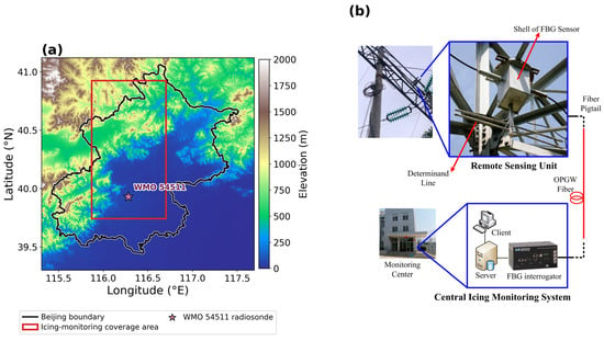
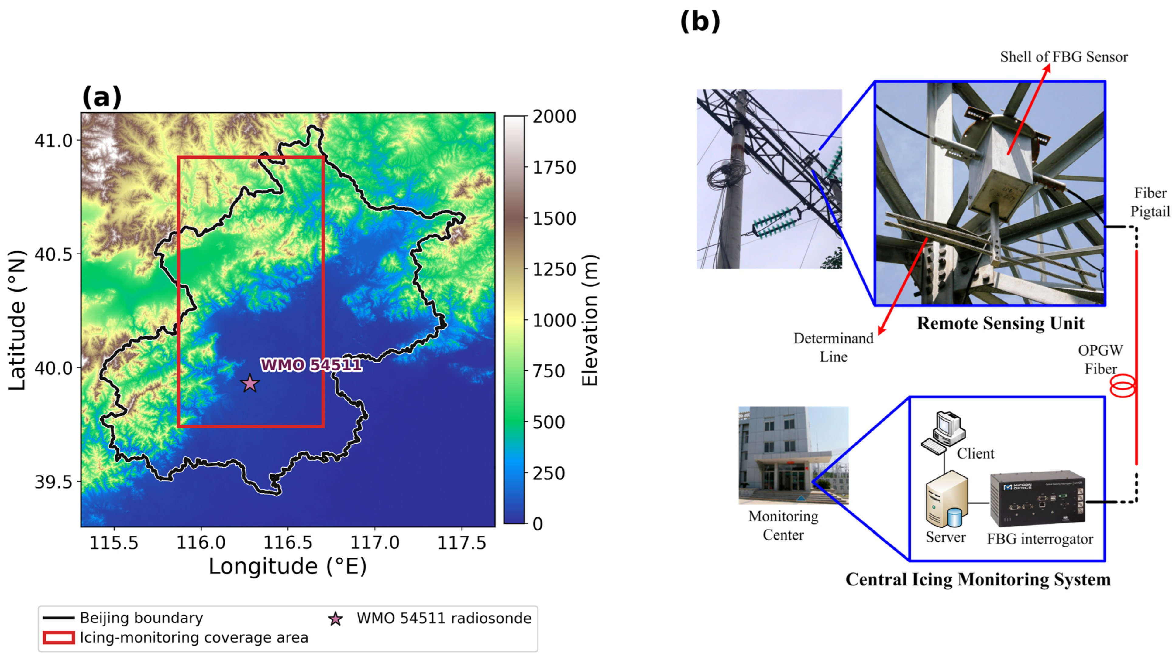
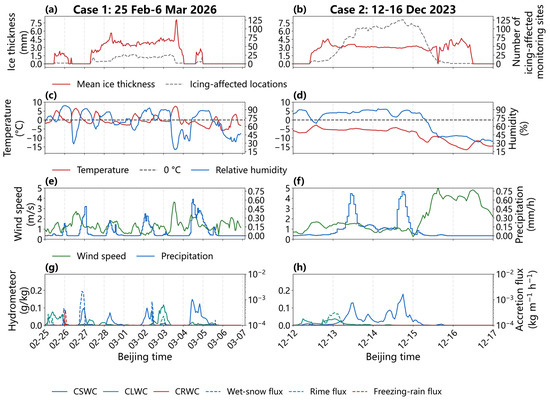
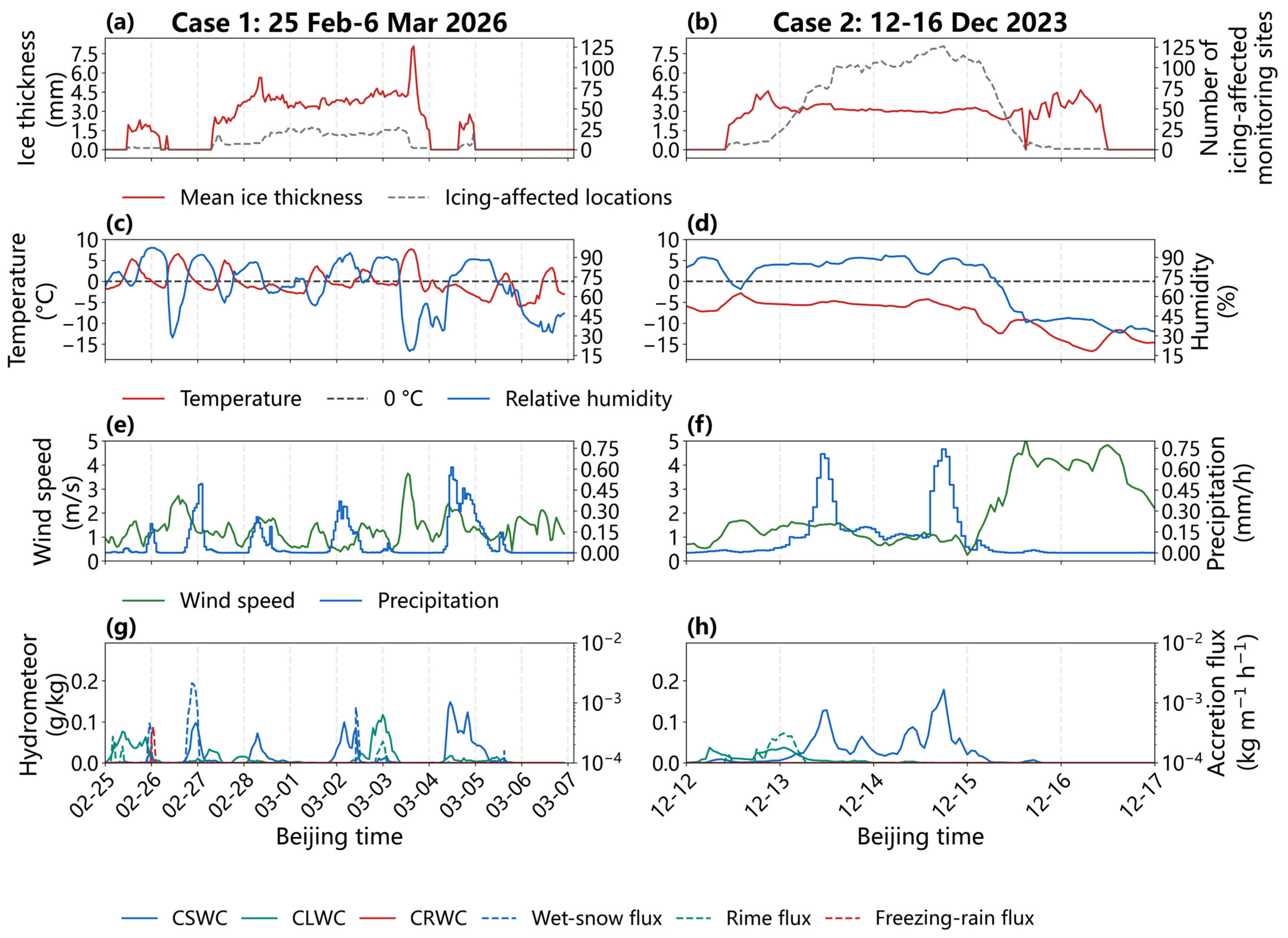
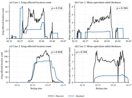
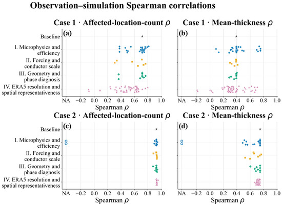
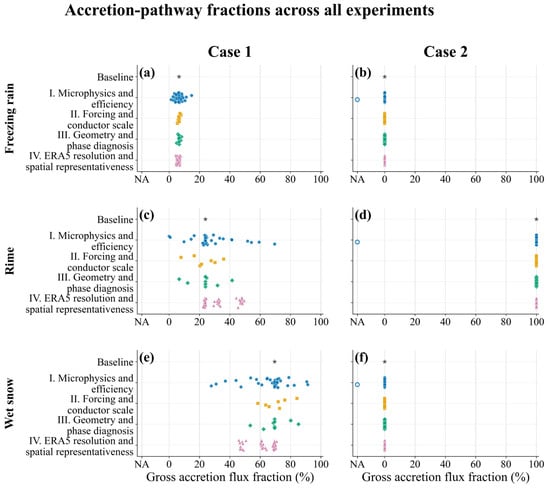
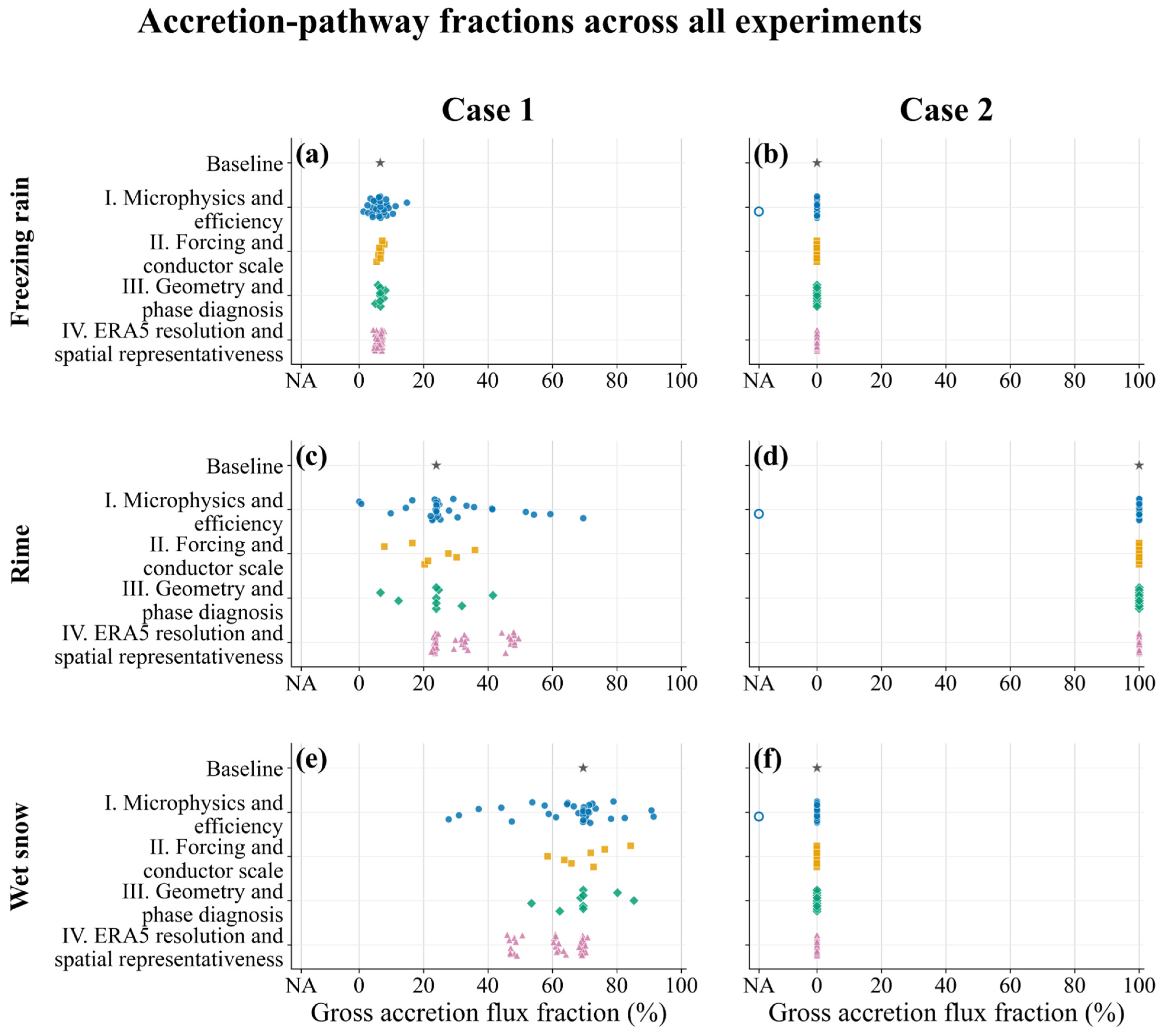
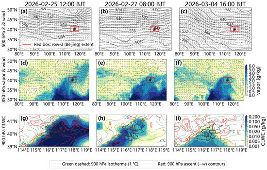
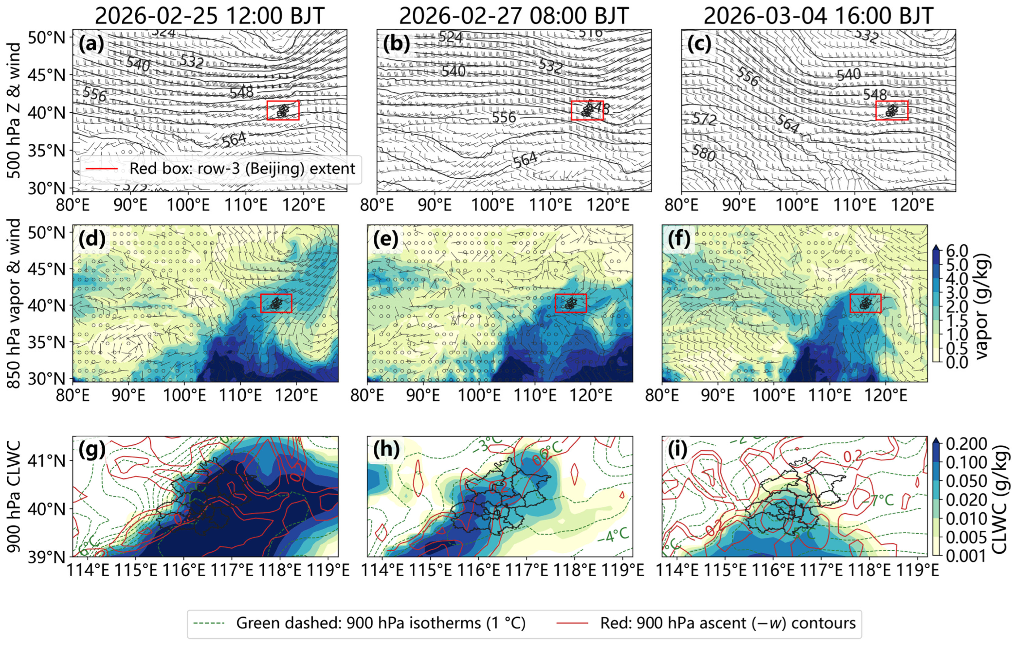
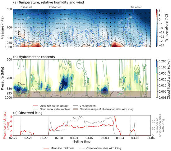
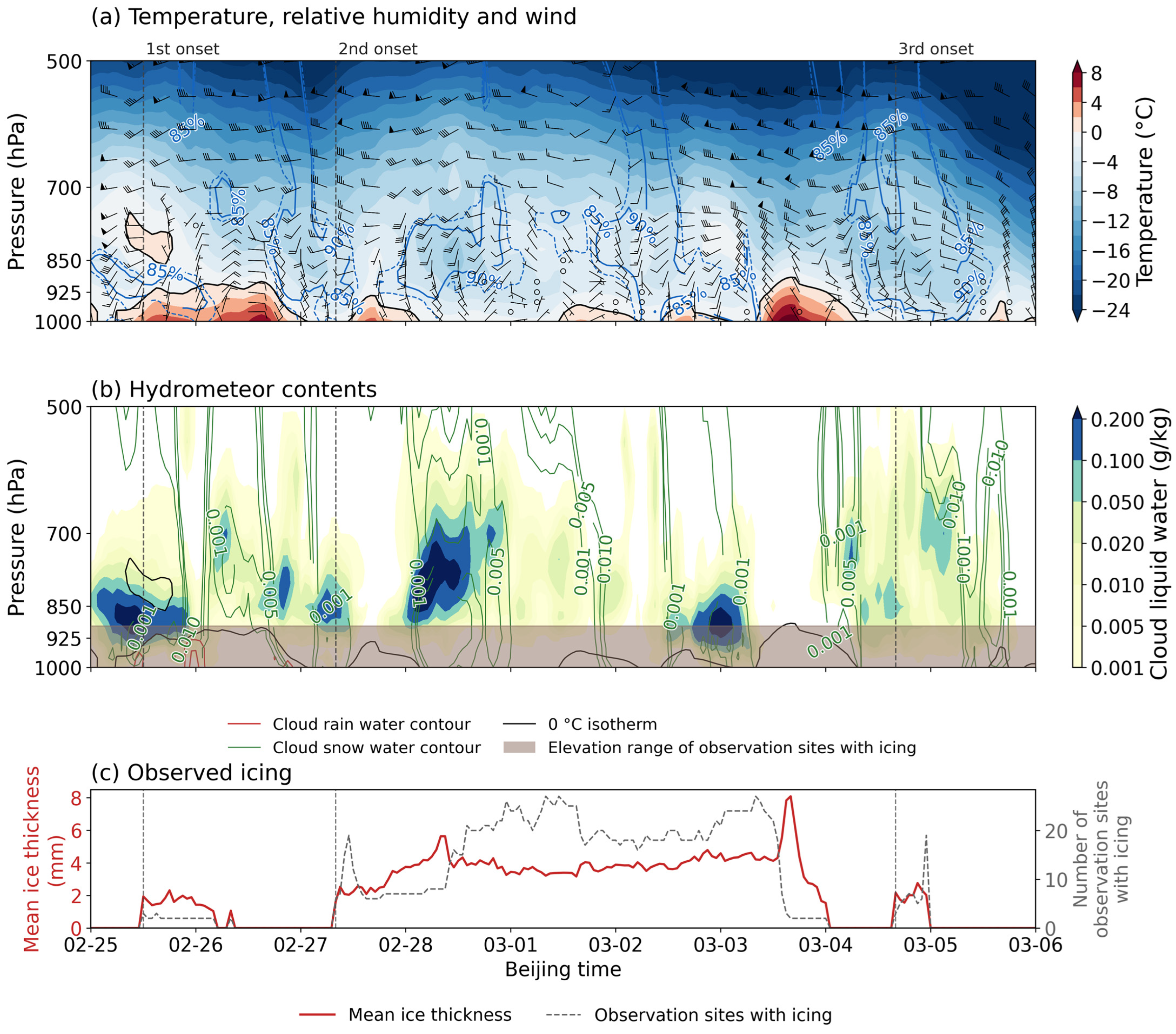
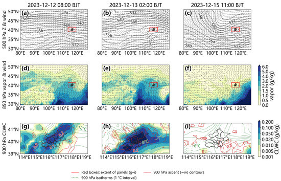
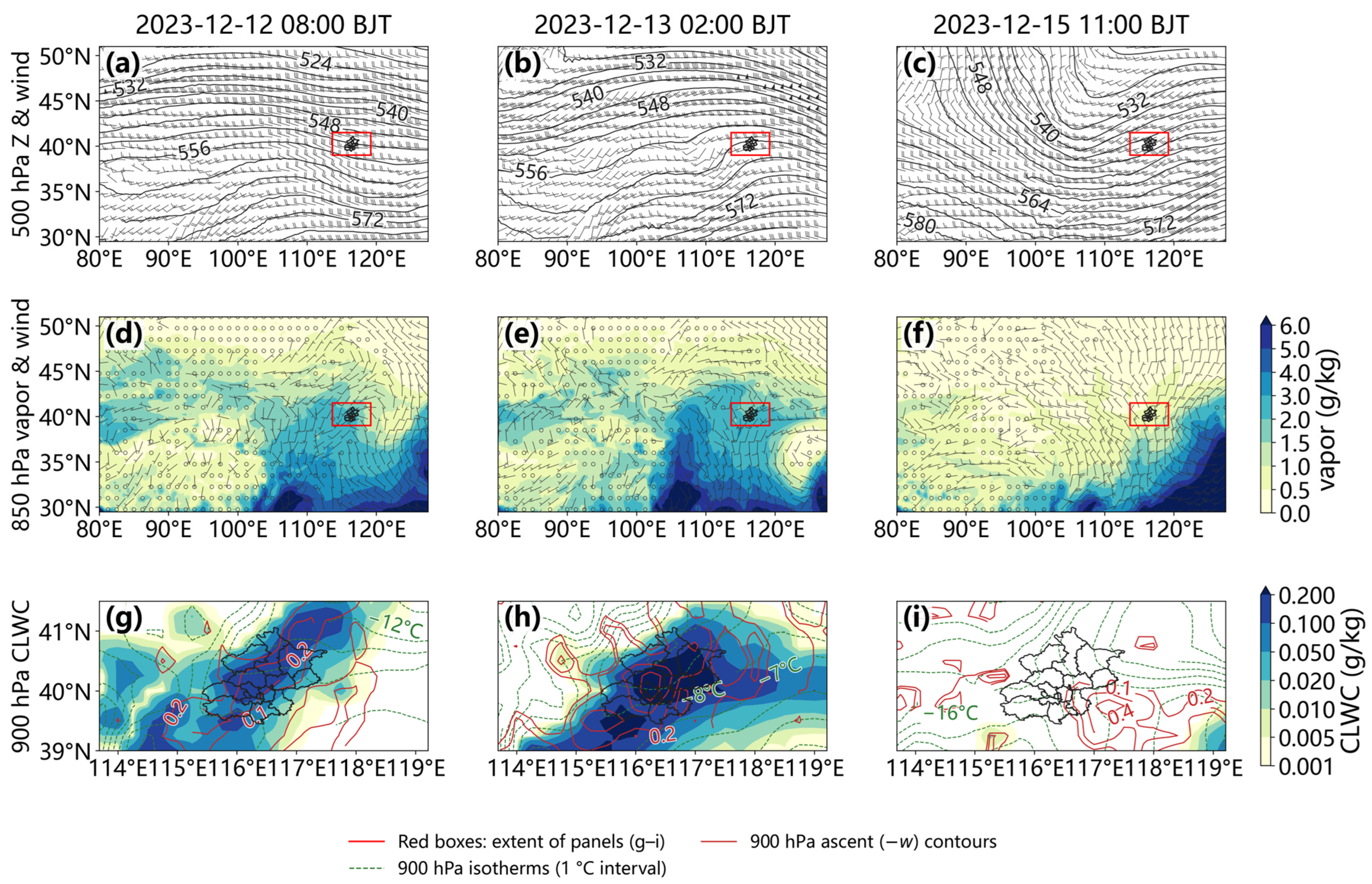
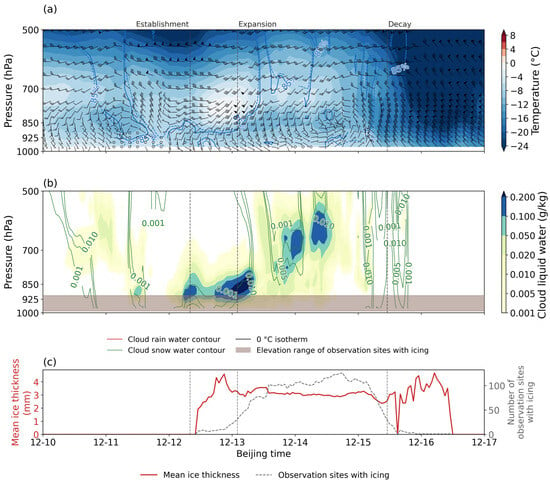
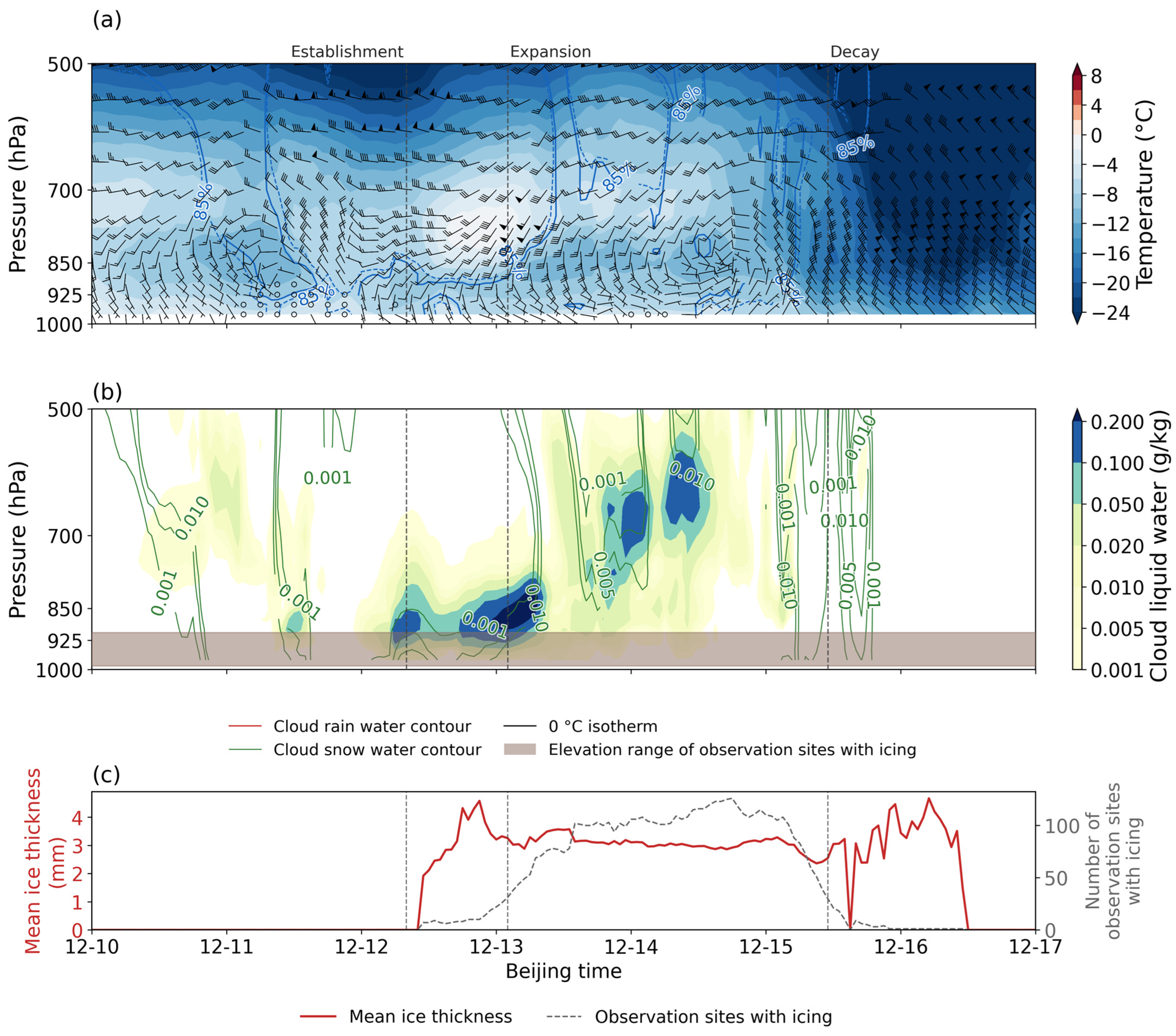
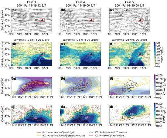
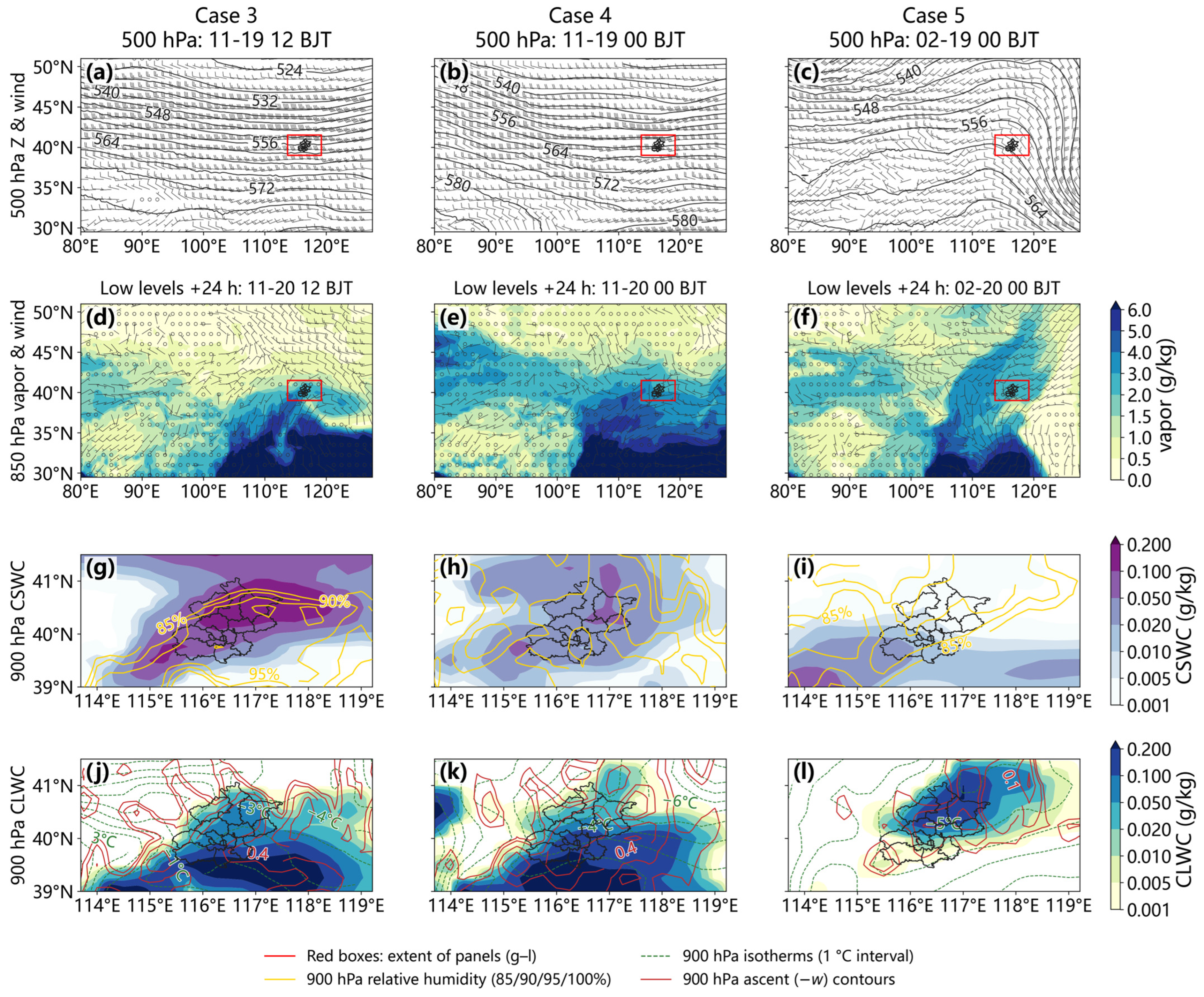
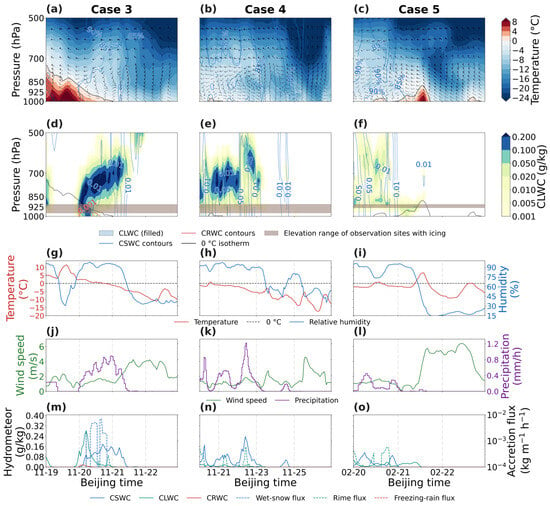
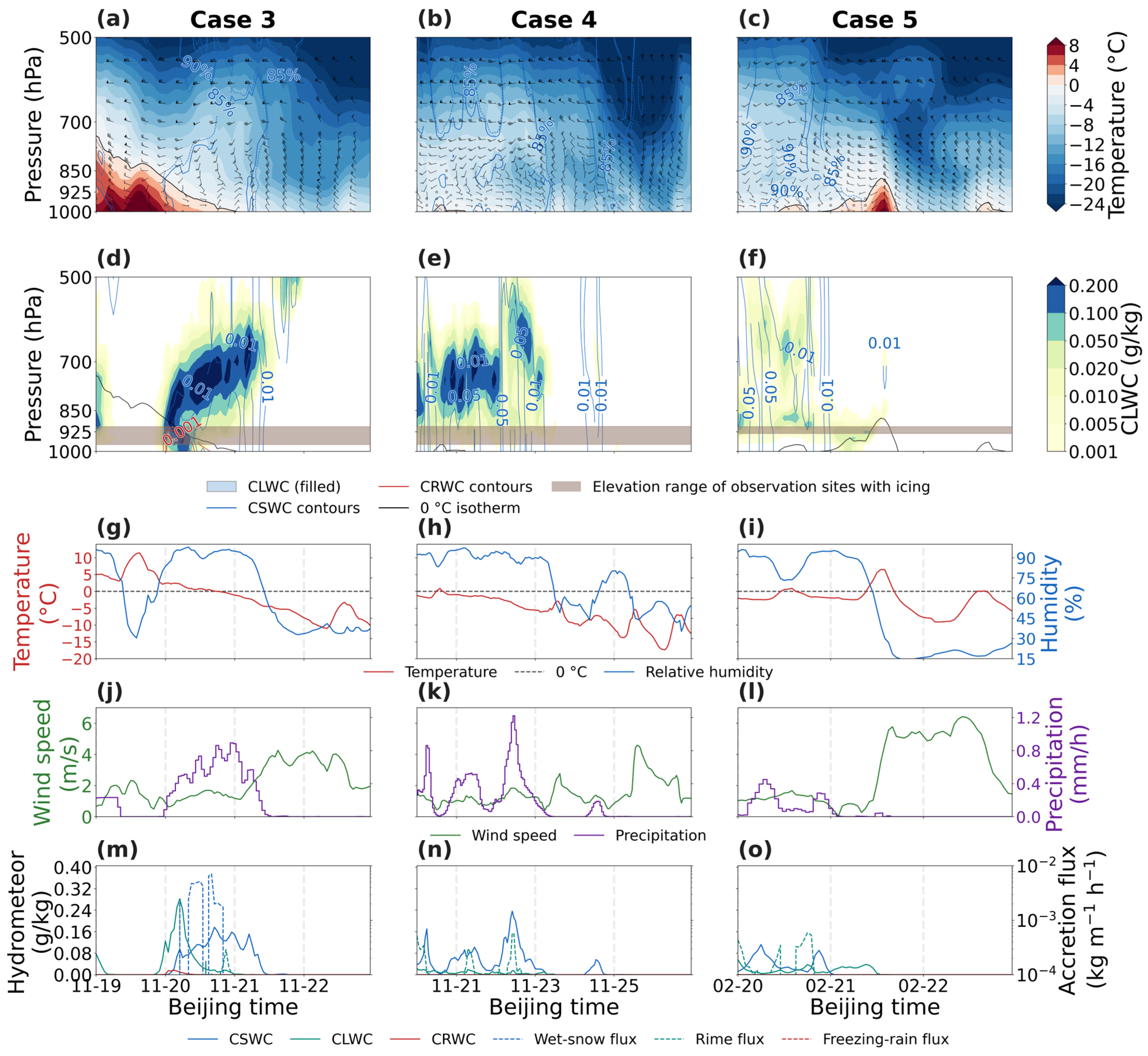
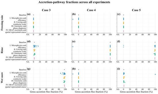
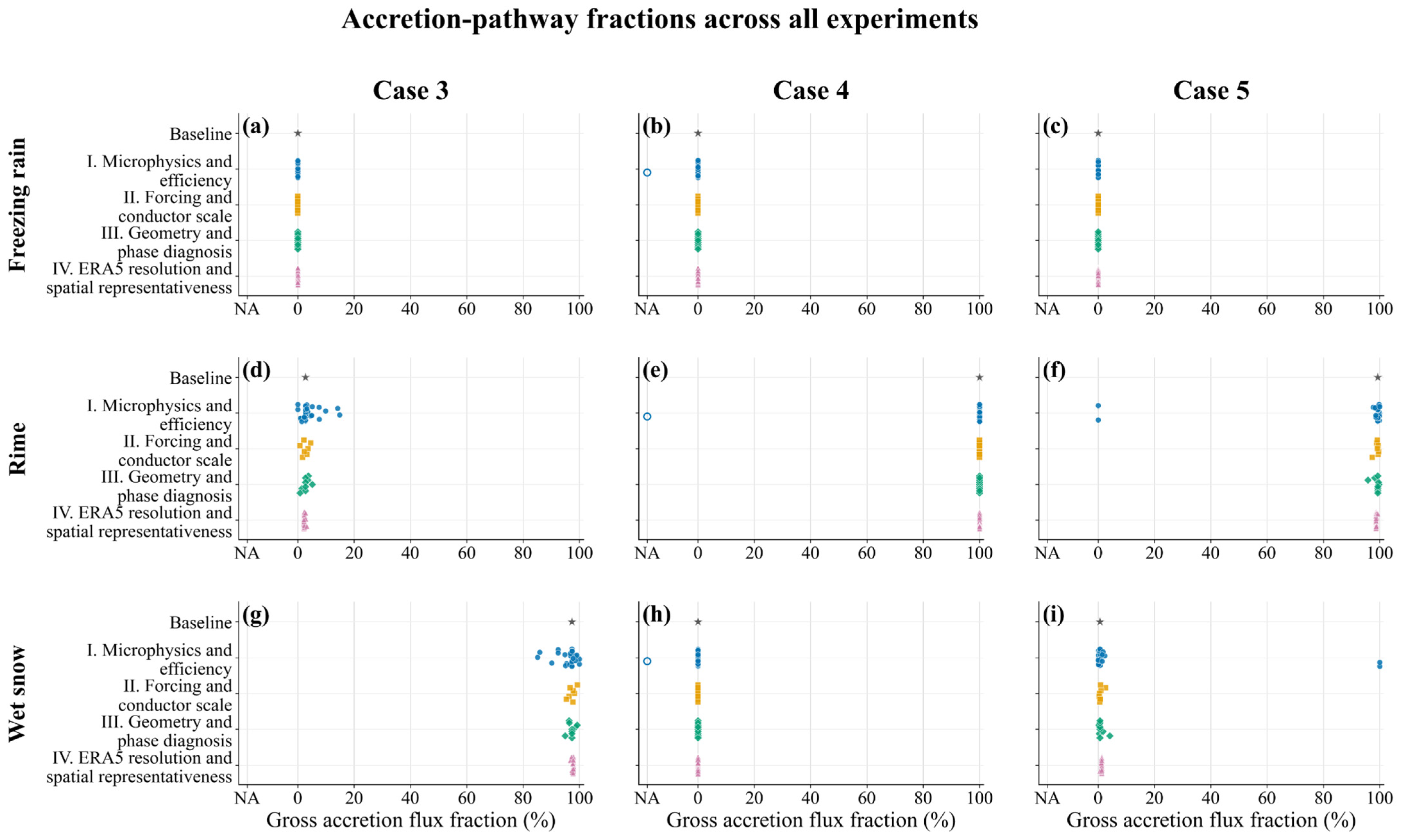
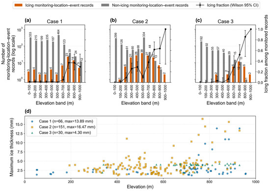
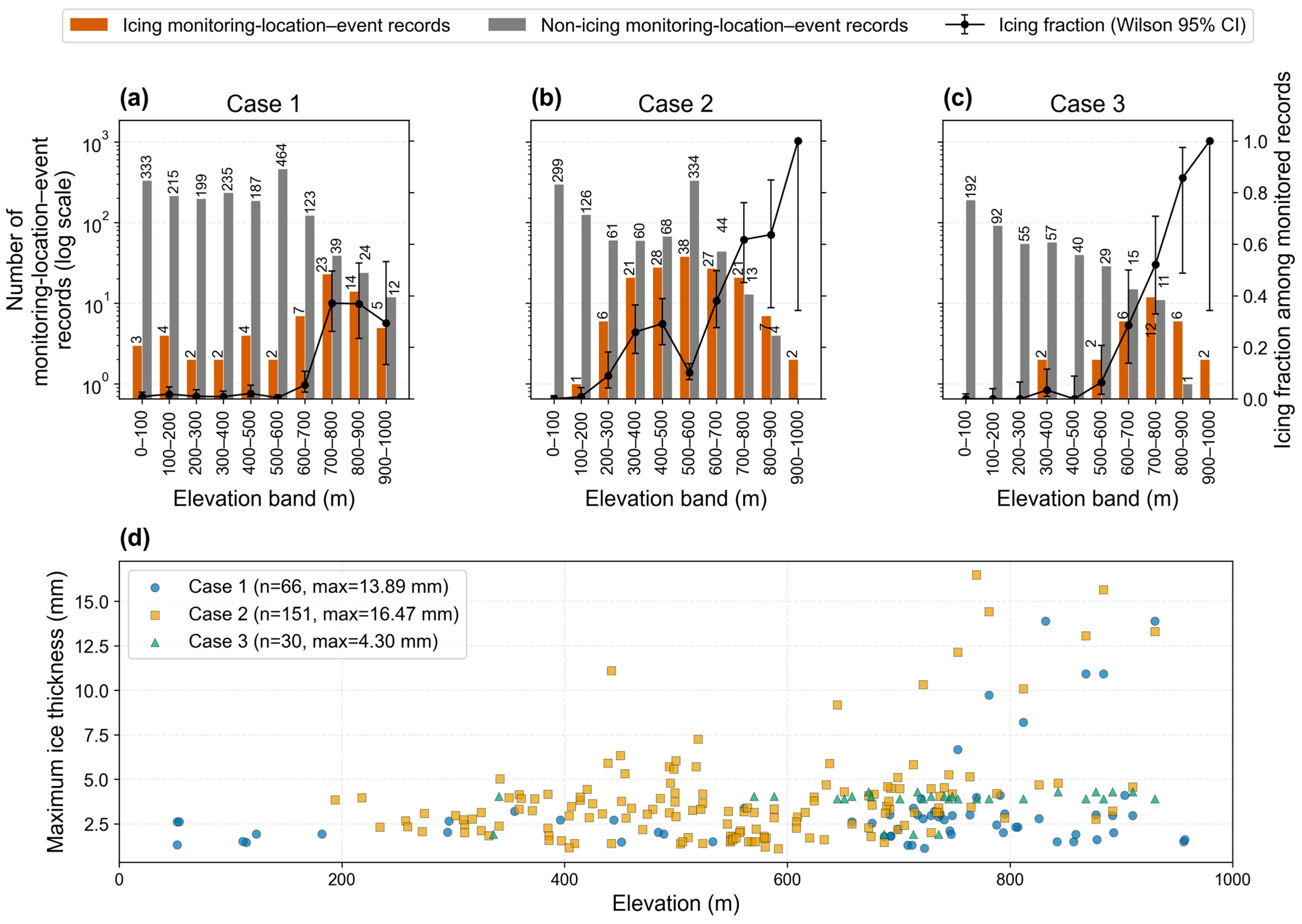
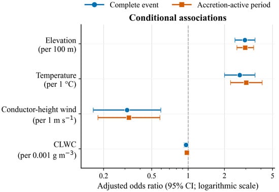
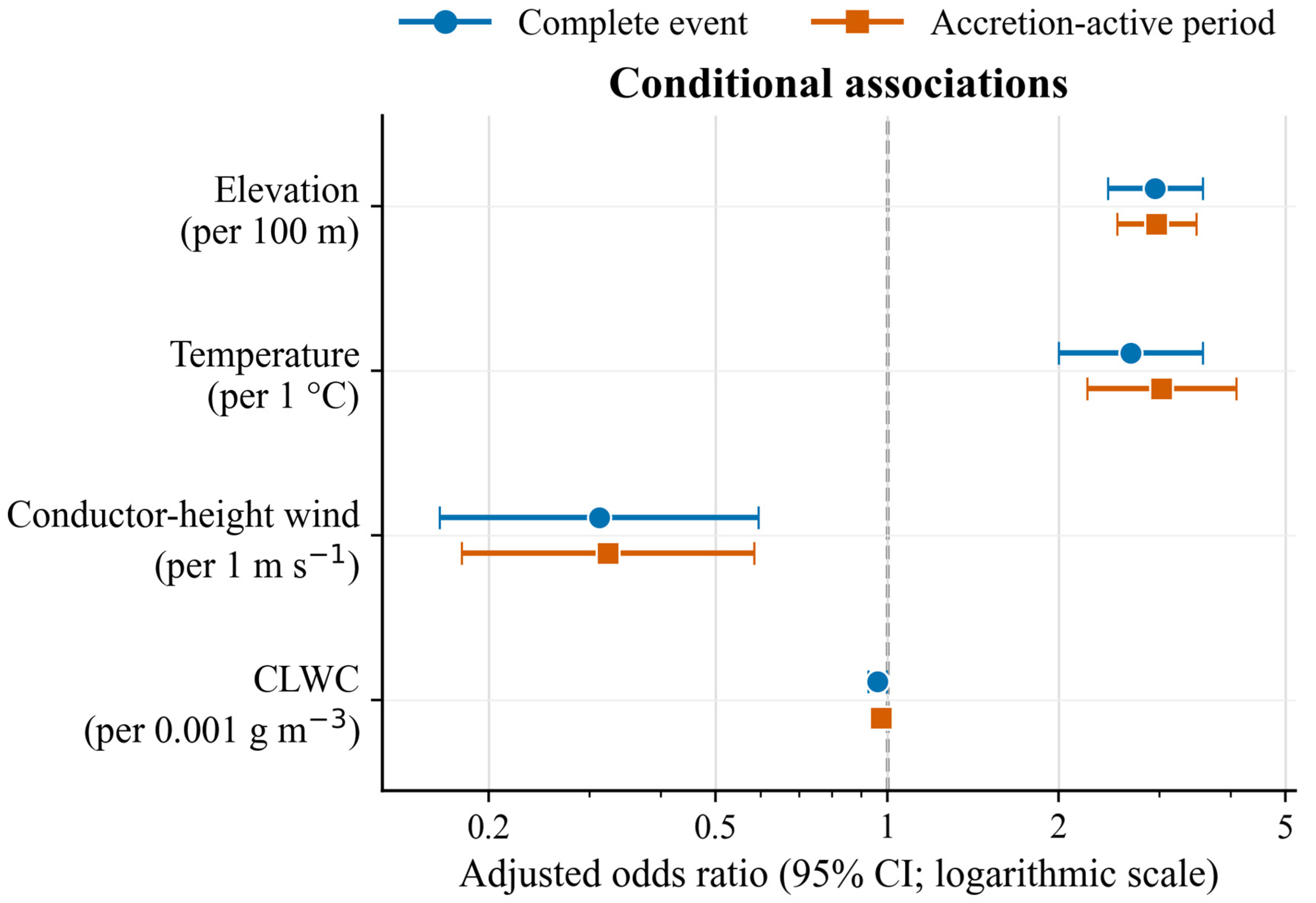
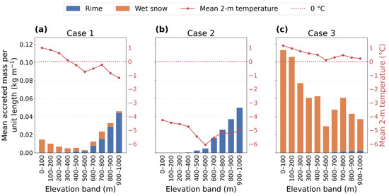

Disclaimer/Publisher’s Note: The statements, opinions and data contained in all publications are solely those of the individual author(s) and contributor(s) and not of MDPI and/or the editor(s). MDPI and/or the editor(s) disclaim responsibility for any injury to people or property resulting from any ideas, methods, instructions or products referred to in the content. |
© 2026 by the authors. Licensee MDPI, Basel, Switzerland. This article is an open access article distributed under the terms and conditions of the Creative Commons Attribution (CC BY) license.