Spatiotemporal Graph Convolutional Attention Network for Air Quality Index Prediction of Beijing, Shanghai and Shenzhen

Abstract

Accurately forecasting air pollutants concentration can reduce health risks and provide an important reference for environmental governance. This study proposes a new deep learning model, GLA-Net, which aims to achieve high-precision prediction of the air quality index (AQI) of monitoring stations. Specifically, GLSTM-Block is designed to use the GAT module to capture dynamic spatial interaction of AQI, generate spatial semantic features, and then use LSTM to capture the temporal correlation characteristics of these spatial characteristics. This paper uses an LSTM network outside of GLSTM-Block to capture the original temporal characteristics of the input data. Then, the temporal characteristics of the LSTM output are added to the dynamic spatiotemporal features of the GLSTM-Block to obtain the final spatiotemporal features as the input of the subsequent temporal attention layer. The temporal attention layer uses a multi-head self-attention mechanism to focus on the impact of the spatiotemporal characteristics of historical air quality data on each prediction time step, and performs AQI prediction through a fully connected layer. Analysis based on measured data from Beijing, Shanghai and Shenzhen shows that the GLA-Net model has significant advantages in predicting single-step and multi-step changes in AQI. The study found that although the model has a large absolute error in predicting concentrations in highly polluted areas, it can better grasp the trend of changes. This feature is particularly evident in Beijing (AQI mean 64.289), with root mean square error (RMSE) of 12.716 and index of agreement (IA) of 0.983.

1. Introduction

China’s rapid industrialization and population growth have led to a continuous decline in air quality, posing a major threat to public health and economic development [1]. To effectively address this challenge, accurate prediction of air quality has become a top priority [2]. Although the concentration of a single pollutant can reflect some air conditions, it is difficult to provide a comprehensive air quality assessment for the public and decision makers [3]. The AQI integrates data on Several pollutants, including PM_2.5, PM₁₀, CO, SO₂, O₃ and NO₂, and converts them into a single indicator based on the national ambient air quality standard, thereby intuitively presenting the comprehensive air quality status [4]. However, due to the dynamic, nonlinear and non-stationary features of the atmospheric environment system, accurate prediction of AQI still faces many challenges, which makes it particularly important to build an applicable prediction model [5,6].

At present, there are two main methods for AQI prediction: one is numerical simulation based on atmospheric environmental theory, which achieves prediction by simulating the migration, transformation and deposition process of air pollutants [7]; and the other is statistical learning method, which uses data mining technology to identify potential laws from multi-source heterogeneous historical data and establish a prediction model for the spatiotemporal changes in pollutant concentration [8].

Numerical simulation methods occupy an important position in the field of ambient air quality forecasting [9]. Numerical models represented by Model-3/CMAQ, CAMx and WRF-Chem have achieved comprehensive prediction of multiple scales and multiple pollutants [10]. Among them, WRF-Chem significantly reduces the system error through the complete coupling of meteorological and chemical transmission [11]. At the same time, the air quality prediction system independently developed by my country’s scientific research institutions, represented by NAQPMS, has formed a forecasting system adapted to local characteristics [12]. However, the complex atmospheric physical and chemical processes place extremely high demands on computing resources, limiting the application of numerical simulation in real-time prediction [13].

Statistical learning-based prediction techniques have progressively surfaced as a result of the ongoing collection of monitoring data [14]. Early statistical models such as multivariate regression, Kalman filtering and hidden Markov models can reveal the laws of time series data, but they are limited in dealing with periodic fluctuations and sudden changes in AQI. In contrast, new machine learning models have broken through the limitations of linear assumptions and show stronger nonlinear pattern recognition capabilities, but they are still insufficient in model depth and feature extraction [15].

The vigorous development of deep learning has promoted the innovative application of end-to-end models in the field of time series forecasting [16,17]. In AQI forecasting, models such as deep feedforward neural network (DFNN), convolutional neural network (CNN), recurrent neural network (RNN) and its variants long short-term memory (LSTM) and gated recurrent unit (GRU) have shown excellent performance [18,19,20,21]. These models focus on characterizing the nonlinear time-dependent characteristics of the AQI pollution process, but the correlation of spatial dimensions is insufficient.

Recently, transformer-based architectures have emerged as powerful alternatives for air quality prediction, leveraging self-attention mechanisms to capture long-range temporal dependencies more effectively than traditional RNN-based models [22,23,24]. Several studies have demonstrated the superiority of transformer models in capturing complex temporal patterns in pollutant concentration data [25,26,27]. Furthermore, hybrid physics-informed neural networks (PINNs) have gained attention by integrating domain knowledge of atmospheric physics and chemistry into data-driven models, thereby improving prediction accuracy while maintaining physical consistency [28,29]. These approaches effectively address the challenge of limited training data by incorporating established physical laws as constraints. Additionally, multi-modal fusion approaches that incorporate satellite imagery, meteorological data, and ground-level monitoring information have shown promise in enhancing spatial coverage and prediction performance, particularly in regions with sparse monitoring networks [30,31].

One important aspect of geospatial study that cannot be disregarded is the nonlinear interdependence across areas [32]. In view of the complex spatiotemporal characteristics of the AQI change process, researchers have proposed a hybrid architecture that integrates multiple basic models [33]. For instance, the accuracy of Shanghai’s AQI daily forecast has been increased by combining the time series modeling benefits of LSTM with the spatial feature extraction capacity of CNN [34]. Nevertheless, due to discrete and irregular distribution characteristics of air quality monitoring stations, the collected AQI data exhibits non-Euclidean spatial properties. Traditional CNN can only process Euclidean spatial structure data with a fixed grid structure. When applied to non-Euclidean spatial structure data, the original data needs to be converted to a certain extent, and the structural information cannot be fully utilized. Therefore, there are major defects in the spatial feature extraction of AQI data based on CNN [35].

Recent research has extended CNN to GCN that can handle non-Euclidean spatial structured data, and has been effectively utilized for prediction tasks for time series data, including air pollutant prediction [36,37]. However, when conventional GCN architectures process spatiotemporal data, they often suffer from spatial and temporal data redundancy issues. Specifically, GCNs tend to aggregate information from all neighboring nodes and time steps equally, without distinguishing the varying importance of different spatial locations and temporal periods [38,39]. This leads to the inclusion of irrelevant or weakly correlated information, which may dilute critical features and reduce prediction accuracy.

To address these challenges, several dynamic GCN variants have been proposed in recent years. Temporal Graph Convolutional Networks (T-GCN) integrate GRU with graph convolution to capture temporal dynamics, but still rely on predefined static spatial graphs [40]. Spatial-Temporal Graph Convolutional Networks (STGCN) employ temporal convolutions alongside spatial graph convolutions, yet their fixed receptive fields limit adaptability to varying correlation patterns [41]. Diffusion Convolutional Recurrent Neural Networks (DCRNN) model traffic diffusion processes using bidirectional random walks, though the computational complexity increases significantly with network scale [42]. Attention-based Spatial-Temporal Graph Convolutional Networks (ASTGCN) incorporate spatial and temporal attention modules, but the separate processing of spatial and temporal features may not fully capture their intricate interactions [43]. While these methods have made progress in modeling dynamic spatiotemporal relationships, they often require complex graph structure learning or predefined adjacency matrices, and may still struggle with effectively filtering redundant information across both spatial and temporal dimensions simultaneously.

In contrast, more recent research has increasingly adopted attention mechanisms that can selectively focus on spatially and temporally relevant information. Attention mechanisms effectively filter out redundant data and concentrate on the most informative features. The advantage of GAT is that they can solve the problem of data redundancy and dynamic spatial correlation through end-to-end learnable attention weights without requiring predefined graph structures, which brings new inspiration to this study [44]. Building on this understanding, in pollution prediction research, there are three key factors that require special attention: (1) Considering the diffusion characteristics of pollutants, the dynamic correlation between all monitoring stations must be considered during the spatial feature extraction process, while avoiding spatial data redundancy; (2) Due to the dynamic and periodic changes in pollutant concentrations, accurate modeling of temporal correlation is crucial, while filtering out temporally irrelevant information; (3) In the multi-station atmospheric pollution prediction task, extracting the long-term spatiotemporal dependency features of sequence data is also critical. In light of these challenges, this study proposes a novel spatiotemporal graph attention network, GLA-Net, for air quality index (AQI) prediction, and introduces the following innovations to address the problems of spatiotemporal redundancy and difficulty in extracting correlations:

(1)

Integrated dual-attention GLSTM-block with coupled spatial-temporal processing. Unlike conventional sequential GAT and LSTM architectures, our GLSTM-block tightly couples spatial and temporal attention by feeding GAT’s spatial attention weights directly into LSTM gating mechanisms. This design filters out spatial redundancy before time processing, thus preventing the spread of irrelevant information.

(2)

Temporal attention for dynamic historical correlation and redundancy filtering. The temporal attention mechanism calculates correlation between historical inputs and predicted values through query–key–value transformations, dynamically identifying the most impactful historical time steps for current predictions. Unlike standard temporal attention that treats all history equally, our mechanism explicitly filters temporal redundancy by assigning differentiated weights that suppress weakly correlated information while emphasizing critical historical patterns, effectively modeling both periodic variations and sudden changes in AQI time series.

(3)

Dense connectivity with layer normalization for enhanced feature propagation. This study integrates dense connection structures and layer normalization to address information degradation in deep architectures. Dense connections create direct inter-layer pathways that enable multi-scale feature fusion, suppress gradient vanishing, and promote feature reuse across network depth. Layer normalization stabilizes the feature distribution at each layer, mitigating internal covariate shift and improving training convergence [37,45]. This integrated design ensures robust propagation of the spatiotemporal features extracted by the dual-attention mechanism, enhancing both model trainability and prediction performance.

(4)

This paper selects AQI as the prediction target for experimental verification. Experimental results in three cities show that the proposed prediction model outperforms other cutting-edge models in terms of RMSE, mean absolute error (MAE), and IA metrics. In addition, GLA-Net exhibits good dynamic characteristics, especially in areas with high concentrations of air pollutants, and can more accurately predict the changing trend of AQI.

2. Study Area and Dataset

2.1. Study Area

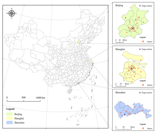
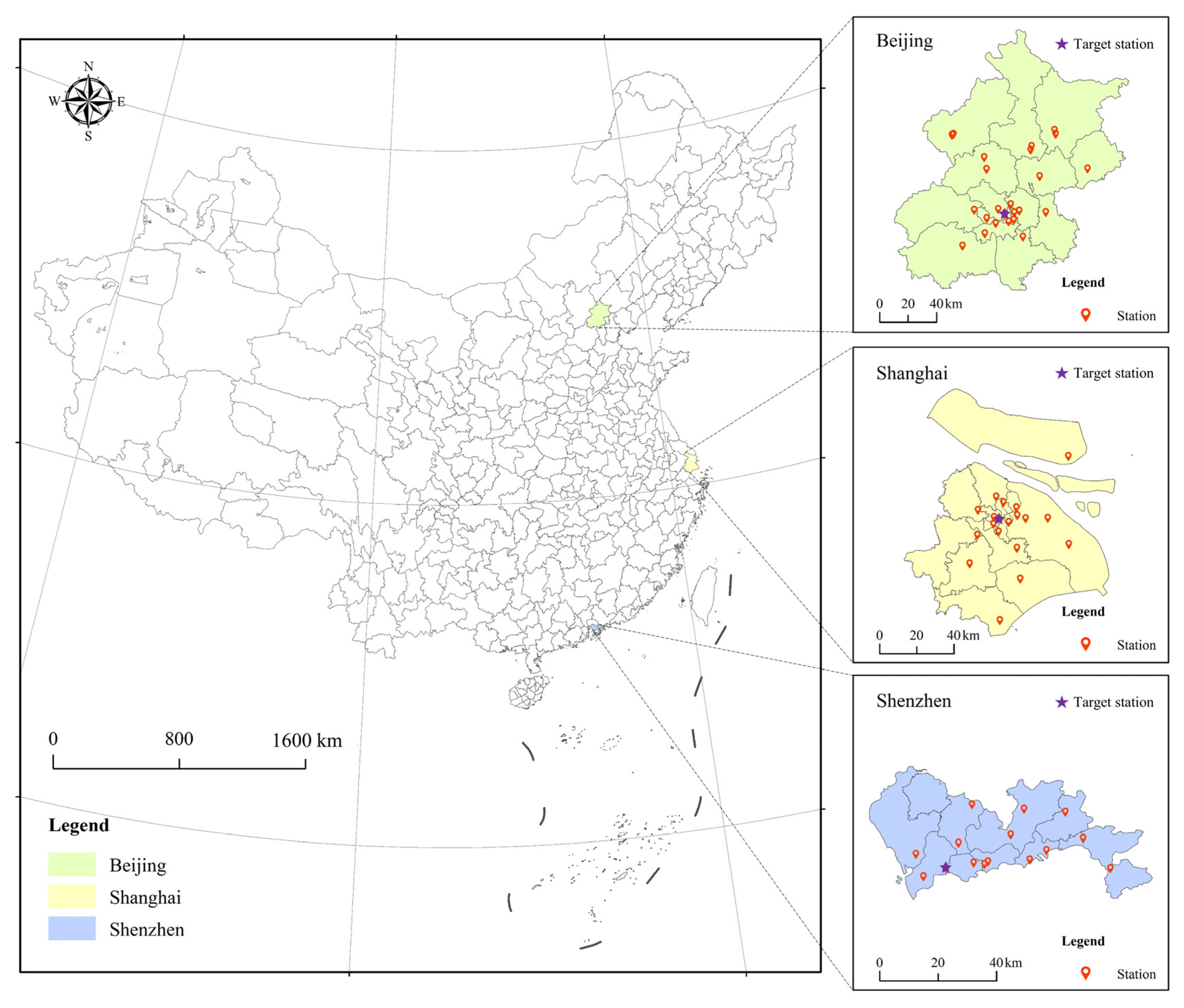
Figure 1 displays the locations of the research items, Beijing, Shanghai, and Shenzhen. In Beijing, the AQI frequently above the norm in the fall and winter, particularly during calm breezes and unfavorable temperatures, which might be harmful to human health [46]. Beijing’s air quality has improved recently because of the adoption of popular regulations. Shanghai is located at the mouth of the Yangtze River and is the economic and financial center of the Yangtze River Delta region [47]. For the sake of protecting the atmospheric environment in the Yangtze River Delta, it is very beneficial to examine the trend of changes in Shanghai’s air quality. The Pearl River Delta’s eastern region is home to Shenzhen. It is a frontier city of science and technology and innovation in China, known for its rapid urbanization and industrialization [48]. Strict environmental protection laws have helped Shenzhen reduce air pollution to some degree in recent years, but it still persists. The air quality conditions in Beijing, Shanghai, and Shenzhen not only reflect the level of development and environmental governance outcomes of their respective cities, but also provide crucial scientific foundation for air environment governance in various regions. This is because Beijing, Shanghai, and Shenzhen are the central cities of the Beijing–Tianjin–Hebei, Yangtze River Delta, and Pearl River Delta regions, and their geographical locations are relatively independent and unique.

Figure 1. Area of study.

2.2. Description of the Data

Three cities’ historical pollution concentrations and weather data from 1 January–31 December 2021, were utilized in this investigation. A one-dimensional feature vector comprising contaminants and climatic variables is used to represent the hourly sample data that each monitoring station in each city provides. The statistical results of the data for Beijing are presented in an understandable way in Table 1. One of the 13 pollutants and 11 meteorological characteristics used for this study is SO₂_24h, which represents the 24 h sliding average of SO₂ concentration. The meteorological data is available on the open weather website (https://openweathermap.org/, accessed on 1 December 2022), and the pollution data is available on the open website (https://quotsoft.net/air/, accessed on 1 December 2022).

Table 1. Data information.

Parameters	Beijing (1006A Station)			Shanghai (1147A Station)			Shenzhen (1358A Station)
	Max	Min	Missing (%)	Max	Min	Missing (%)	Max	Min	Missing (%)
Temperature $\left(\mathrm{K}\right)$	312.3	254.6	0	309.7	265.9	0	309.3	279.8	0
Dew point	300.4	240.4	0	304.1	254.6	0	306.2	265.3	0
Sensible temperature	315.1	247.9	0	316.8	258.9	0	316.3	276.1	0
Min temperature	309.8	250.1	0	309.2	265.3	0	307.6	279.2	0
Max temperature	313.1	254.8	0	310.3	266.4	0	309.4	281.5	0
Pressure $\left(\mathrm{P}\mathrm{a}\right)$	1048	988	0	1042	985	0	1031	994	0
Humidity $\left(\mathrm{\%}\right)$	100	10	0	100	15	0	99	24	0
Wind speed $(\mathrm{m}\mathrm{i}\mathrm{l}\mathrm{e}\mathrm{s}/\mathrm{h})$	8.59	0.02	0	17	0	0	9.7	0	0
Wind direction $(°)$	360	0	0	360	0	0	360	0	0
Cloudiness	100	0	0	100	0	0	100	0	0
Weather id	804	200	0	804	200	0	804	500	0
AQI	500	8	2.72	500	8	3.57	248	6	4.72
PM2.5 $(\mathsf{\mu }\mathrm{g}·{\mathrm{m}}^{-3})$	663	1	2.12	178	1	2.03	198	1	4.81
PM2.5_24h $(\mathsf{\mu }\mathrm{g}·{\mathrm{m}}^{-3})$	232	2	1.16	106	2	0.74	93	1	1.68
PM10 $(\mathsf{\mu }\mathrm{g}·{\mathrm{m}}^{-3})$	7093	1	3.81	741	1	2.79	292	1	3.27
PM10_24h $(\mathsf{\mu }\mathrm{g}·{\mathrm{m}}^{-3})$	1771	4	1.17	401	9	0.74	151	3	1.15
SO2 $(\mathsf{\mu }\mathrm{g}·{\mathrm{m}}^{-3})$	51	1	1.79	349	1	1.35	21	1	2.72
SO2_24h $(\mathsf{\mu }\mathrm{g}·{\mathrm{m}}^{-3})$	51	1	1.15	20	1	0.74	14	3	1.15
NO2 $(\mathsf{\mu }\mathrm{g}·{\mathrm{m}}^{-3})$	126	1	1.78	154	3	1.52	232	1	2.23
NO2_24h $(\mathsf{\mu }\mathrm{g}·{\mathrm{m}}^{-3})$	94	2	1.15	126	5	0.74	138	4	1.15
O3 $(\mathsf{\mu }\mathrm{g}·{\mathrm{m}}^{-3})$	1200	1	4.12	281	5	1.41	259	1	4.46
O3_24h $(\mathsf{\mu }\mathrm{g}·{\mathrm{m}}^{-3})$	1200	2	1.15	281	13	0.74	264	4	1.15
CO $(\mathrm{m}\mathrm{g}·{\mathrm{m}}^{-3})$	5	0.1	1.93	3.2	0.1	1.62	1.6	0.1	2.82
CO_24h $(\mathrm{m}\mathrm{g}·{\mathrm{m}}^{-3})$	2.5	0.1	1.15	1.9	0.1	0.74	1	0.2	1.15

2.3. Data Preprocessing

The following preprocessing was done on each station’s pollution and meteorological data across the three cities. Initially, all data were kept since the percentage of missing data was less than 5%, and linear interpolation was used to fill in the missing numbers. We carried out numerical mapping one by one for non-numerical meteorological parameters (such weather conditions). Lastly, all data were normalized to the range of [0, 1] using the Min-Max scaling approach [49]. This normalization is necessary because the input features (e.g., temperature, humidity, pollutant concentrations) have different scales and units, which could cause features with larger numerical ranges to dominate the model training process. Normalization ensures that all features contribute equally to the model and accelerates convergence by improving numerical stability during gradient descent optimization. To maintain the temporal continuity of the time series data, the dataset was split chronologically without shuffling into three sets: a training set (70%), a validation set (15%), and a test set (15%). This 70-15-15 split ratio is commonly adopted in time series prediction tasks, ensuring sufficient training samples while providing adequate data for model validation and independent testing [50]. The training set was used for model parameter learning, the validation set for hyperparameter tuning and preventing overfitting, and the test set for final performance evaluation.

3. Methodology

3.1. Explanation of the Difficulty of Air Quality Prediction

Currently, AQI prediction is a sequence prediction issue with time and space dimensions. That is, forecast the AQI of the target monitoring station in the area for the next time interval based on the historical data on air pollutant concentrations for the current time interval [51]. Based on previous research results, in order to accurately grasp the geographic spatial correlation [52], this paper defines the monitoring stations and pairwise connections as $G=(V,E,A)$, where $V$ represents the node set, $E$ represents the edge set, $V=R^{N\times N}$ represents the adjacency matrix, that is, it represents the proximity between any pair of nodes, and $N$ represents the number of nodes. As shown in Figure 2, this paper abstracts each monitoring station as a node in the graph and the pairwise connections of the monitoring stations as edges. The adjacency matrix A is constructed using the average distance threshold method: (1) Distance Calculation: First, we calculate the Euclidean distance between the monitoring stations based on their geographical coordinates (latitude and longitude); (2) Threshold Determination: We calculate the average distance between all pairs of stations, where N is the total number of monitoring stations; (3) Binary Adjacency Relationship Construction: For any two stations, if the distance between them is less than the average distance, we set it to 1 (connected); otherwise, we set it to 0 (disconnected). Assume that the input time step is $n$, the prediction time step is $p$, and $t_i\in \left\{t_1,\cdots ,t_n,\cdots ,t_{n+p}\right\}$. The core of this study is how to reveal the spatiotemporal correlation of highway network traffic data. Therefore, this paper uses GLA-Net to learn the spatiotemporal features hidden in the monitoring site data to achieve accurate prediction of AQI.

Figure 2. Definition of prediction problem. (a) Air pollution stations network; (b) Graph representation.

3.2. Framework Overview

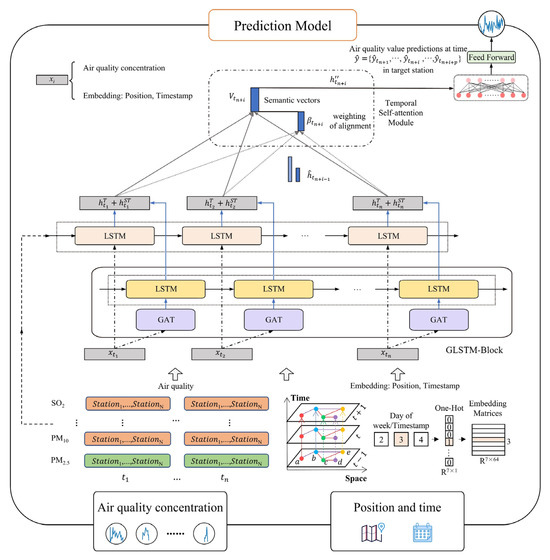
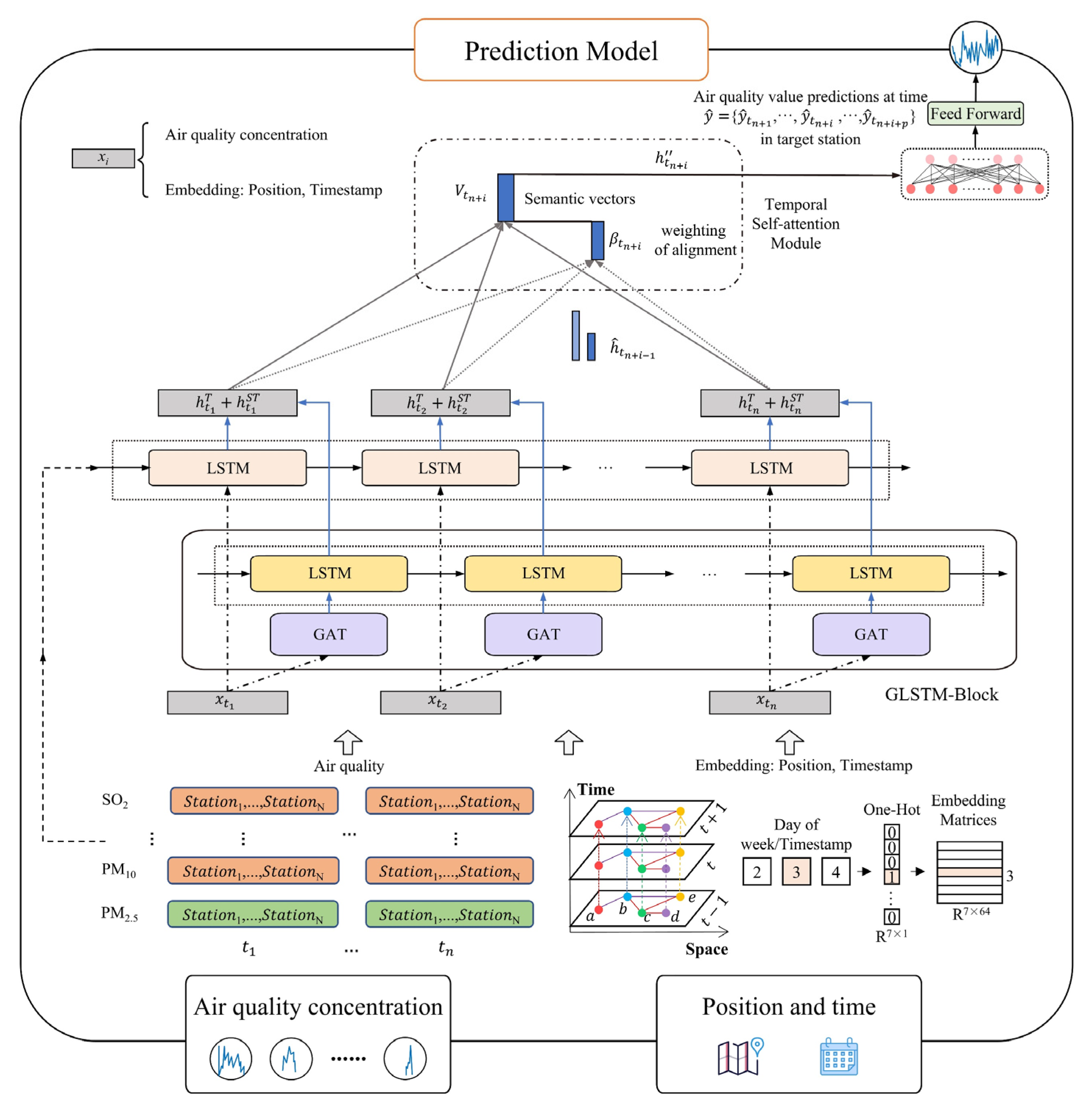
RNN-based models have been widely employed in computer science and related disciplines for time series prediction applications. In the last several years, mainstream pollutant concentration prediction models have mostly adopted LSTM-based structures, using an LSTM to capture time series characteristics from historical data [53]. This structure effectively captures the dynamic changes in time series data and has become the main method for current pollutant concentration prediction. However, the above model ignores the spatial correlation between air quality. Therefore, for spatiotemporal characteristics and long-term AQI prediction, this paper proposes a GLSTM-Block-based model, GLA-Net, as shown in Figure 3. To implement this method, two steps are required.

Figure 3. GLA-Net model architecture.

First, in order to prevent each monitoring station from over-relying on the information of surrounding monitoring stations and to maintain its own personalized time series characteristics, this study employs a dual-pathway architecture where, independent of GLSTM-Block, a separate LSTM branch specifically extracts the time features of the original input data, as shown in Figure 3. In GLSTM-Block, AQI data $x_{t_i}=\left\{x_{t_1},\cdots ,x_{t_n}\right\}$ is fed into the model in a pipeline manner. The dynamic spatial correlation of the air quality data is extracted through GAT in GLSTM-Block to generate high-level spatial semantic features $h_{t_i}^S=\left\{h_{t_1}^S,\cdots ,h_{t_n}^S\right\}$. Then, LSTM is also used to extract the output of GAT to generate the temporal correlation of spatial semantic features $h_{t_i}^{ST}=\left\{h_{t_1}^{ST},\cdots ,h_{t_n}^{ST}\right\}$. Finally, the LSTM output $h_{t_i}^T$ and the GLSTM-Block output $h_{t_i}^{ST}$ are added to obtain the final spatiotemporal features ${\widehat{h}}_{t_i}=\left\{{\widehat{h}}_{t_1},\cdots ,{\widehat{h}}_{t_n}\right\}$, which are later used in the temporal self-attention layer. A task layer and a temporal attention layer come next. The temporal attention layer uses a multi-head self-attention mechanism to focus on the impact of the spatiotemporal elements of historical air quality data on the predicted value of each time step, while the task layer uses a fully connected layer to perform the AQI prediction.

In order to avoid internal covariate shift issues and network information loss, the GLA-Net suggested in this study incorporates dense connections and layer normalization techniques across the network [45,54]. Within GLSTM-Block, we employ dense connections between GAT and LSTM layers to ensure effective feature propagation and reuse. This dense connectivity enables the temporal LSTM to directly access both the raw spatial features and the refined spatial semantic features from GAT, preventing information loss and facilitating gradient flow through the spatiotemporal processing pipeline. For the final integration of the two parallel pathways, we use element-wise addition rather than more complex fusion mechanisms. This design choice serves a specific purpose: the additive combination allows the model to preserve station-specific temporal patterns (from the independent LSTM branch) while incorporating network-wide spatiotemporal dependencies (from GLSTM-Block). Unlike concatenation that would double the feature dimension and require additional projection parameters, or gating mechanisms that would introduce learnable weights to control information flow, simple addition achieves balanced integration without parameter overhead. This ensures that the personalized time series characteristics of individual monitoring stations are maintained alongside the spatially refined features, which is critical for accurate station-level AQI prediction. Each component of the GLA-Net model’s implementation procedure will be thoroughly explained in the sections that follow.

3.3. Embedding Layer

Each node contains three types of data information, including location information, timestamp information and air quality information. The input variable $x_{t_i}=\left\{e_l^{t_i},e_a^{t_i},e_t^{t_i}\right\}$ can be divided into three types of embedded representations, including location embedding $e_l^{t_i}\in R^{N\times d}$, timestamp embedding (hour, week, month) $e_t^{t_i}\in R^{N\times d}$, and air quality information is divided into 24 types, which are embedded in $e_a^{t_i}$. The timestamp and location embedding methods are the same as the Transformer embedding methods, and are mapped to dense matrices through one-hot. The embedding method of each air quality information is completed through linear transformation. For each type of data embedding, the data dimension can be expressed as $d=d_{model}⁄3=$64.

3.4. GLSTM-Block

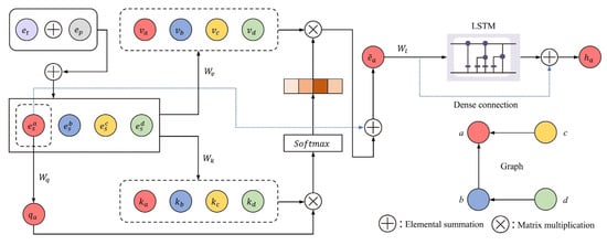
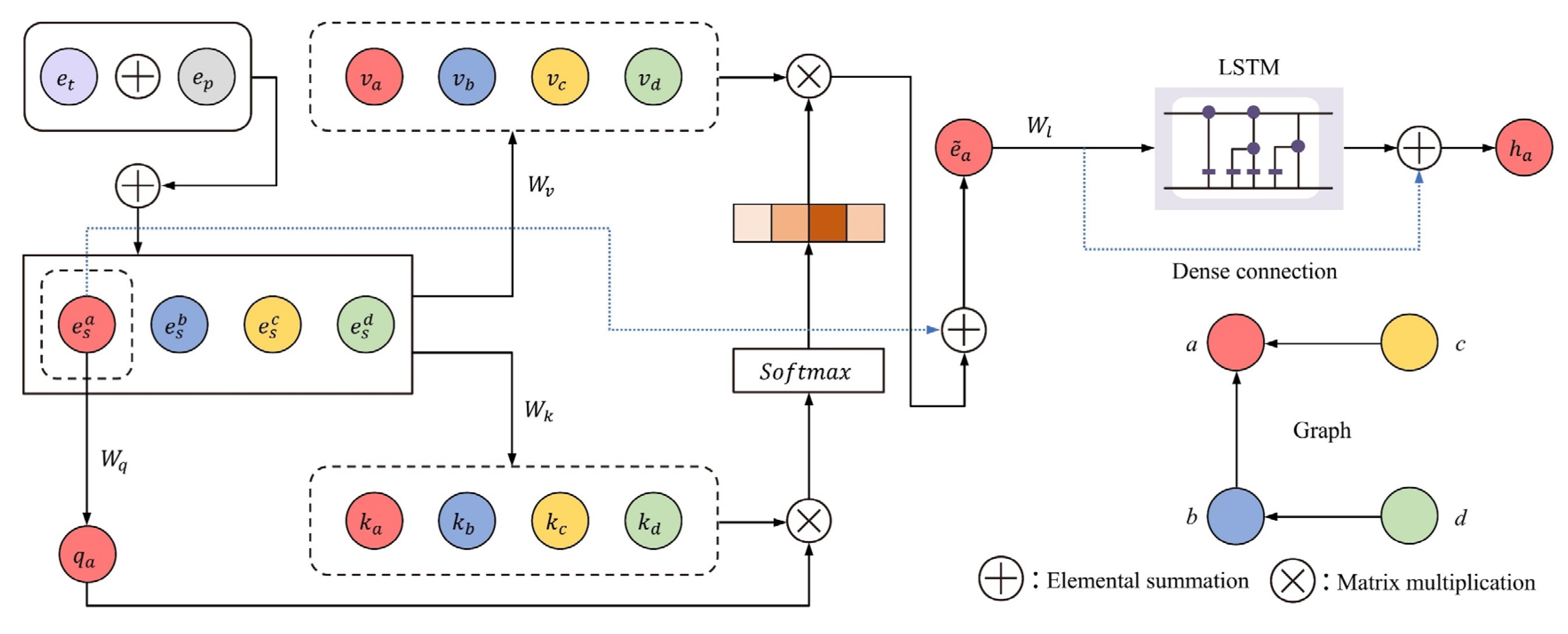
A dynamic spatial feature extractor and a temporal feature extractor are the two main components of GLSTM-Block, as seen in Figure 4. In the spatial dimension, as air pollutants spread, the global air quality has an influence on each monitoring site’s AQI, and the impact weights w vary with time; this is known as dynamic spatial correlation. Multi-layer GAT is used by GLSTM-Block to capture the dynamic spatial correlation. The same station exhibits temporal correlation for several time steps in the temporal dimension, demonstrating the traits of dynamic continuous change, which is what temporal correlation is. This module records the dynamic temporal correlation using multi-layer LSTM. Where $\oplus$ and $\otimes$ represent element-wise summation and matrix multiplication, respectively. Since nonlinear transformation functions will be used a lot in this research, they are first defined as follows:

$$f\left(x\right)=ReLU(xW+b)$$

(1)

where $x$ is the input variable, $W$ and $b$ represent learnable parameters, and $ReLU$ represents the nonlinear activation function.

Figure 4. GLSTM-Block architecture.

3.4.1. Dynamic Spatial Feature Extractor

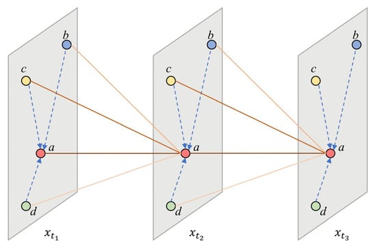
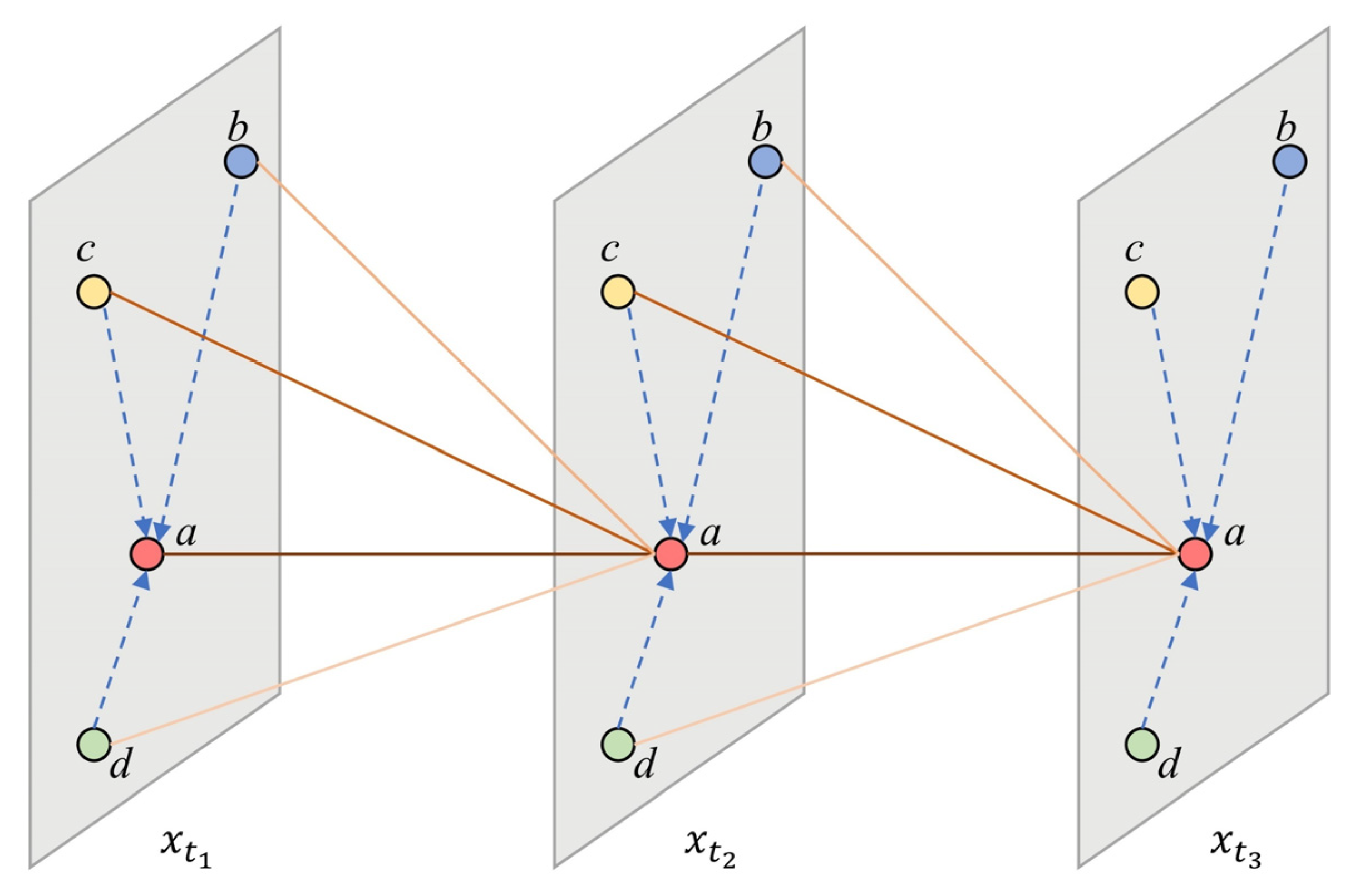
The dynamic spatial correlation of any monitoring site (node) $v_j$ in the area at each time step $t_i$ is extracted using GAT in this research, as seen in Figure 5. For node $v_j$, the input is $e_a^{t_i,v_j}$ and $e_t^{t_i,v_j}$, and the dynamic spatial correlation can be calculated through the multi-head self-attention mechanism. The influence ${\alpha }_{{v,v}_j}^u$ of all nodes $V$ on node $v_j$ can be calculated by the k-th head self-attention, as shown in the following formula:

$${\alpha }_{{v,v}_j}^k={\displaystyle \frac{exp\left(s_{{v,v}_j}^k\right)}{exp\left({\sum }_{v_r}^V{s}_{{v,v}_j}^k\right)}}$$

(2)

where $s_{{v,v}_j}^k$ represents the correlation between node $v_j$ and other nodes $v$.

Figure 5. Dynamic spatial correlation for feature extraction process.

Finding the inner product of the query vector of node $v_j$ with the key vector of $v$ yields the correlation $s_{{v,v}_j}^k$, as indicated by the following formula:

$$s_{{v,v}_j}^k={\displaystyle \frac{f_k^q\left(\left(e_a^{t_i,v_j}+e_t^{t_i,v_j}\right)W_k^q\right)·f_k^k\left(\left(e_a^{t_i,v}+e_t^{t_i,v}\right)W_k^k\right)}{\sqrt{d}}}$$

(3)

where the query vector and the key vector are transformed nonlinearly by $f_k^q$ and $f_k^k$, respectively, and $·$ is the inner product operation.

Following the acquisition of the image weight ${\alpha }_{{v,v}_j}^u$, the hidden state of node $v_j$ is ${\widehat{e}}_{a,k}^{t_i,v_j}$.

$${\widehat{e}}_{a,k}^{t_i,v_j}={\sum }_{v_r}^V{\alpha }_{{v,v}_j}^k{V}_{v_r}^k+e_a^{v_j}$$

(4)

$$V_{v_r}^k=f_k^v\left(\left(e_a^{t_i,v_r}+e_t^{t_i,v_r}\right)W_k^v\right)$$

(5)

where the value vector’s nonlinear transformation function is denoted by $f_k^v$.

After the dynamic spatial correlation of node $v_j$ is calculated by Formula (4), multi-head attention is used. The model may concentrate on data from several stations’ subspaces thanks to multi-head attention. In particular, by parallelizing the M-head attention mechanism and connecting different learned representations, the new hidden state of $v_j$ can be updated by Formula (6).

$${\widehat{e}}_a^{t_i,v_j}=\left[{\widehat{e}}_{a_1}^{t_i,v_j},\cdots ,{\widehat{e}}_{a_M}^{t_i,v_j}\right]W^o$$

(6)

where $W^o$ represents the mapping layer, which helps the model integrate the spatial correlation of all relevant aspects of the highway $v_j$.

At time step $t_i$, the spatial correlation of each monitoring station $v_j$ can be calculated by Formulas (1) to (6), and the output of the overall monitoring station is $h_{t_i}^S$, as shown in the following formula:

$$h_{t_i}^S={\widehat{e}}_a^{t_i}{W}_l$$

(7)

where ${\widehat{e}}_a^{t_i}$ represents the output of the dynamic spatial correlation extractor.

3.4.2. Dynamic Temporal Feature Extractor

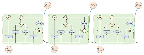
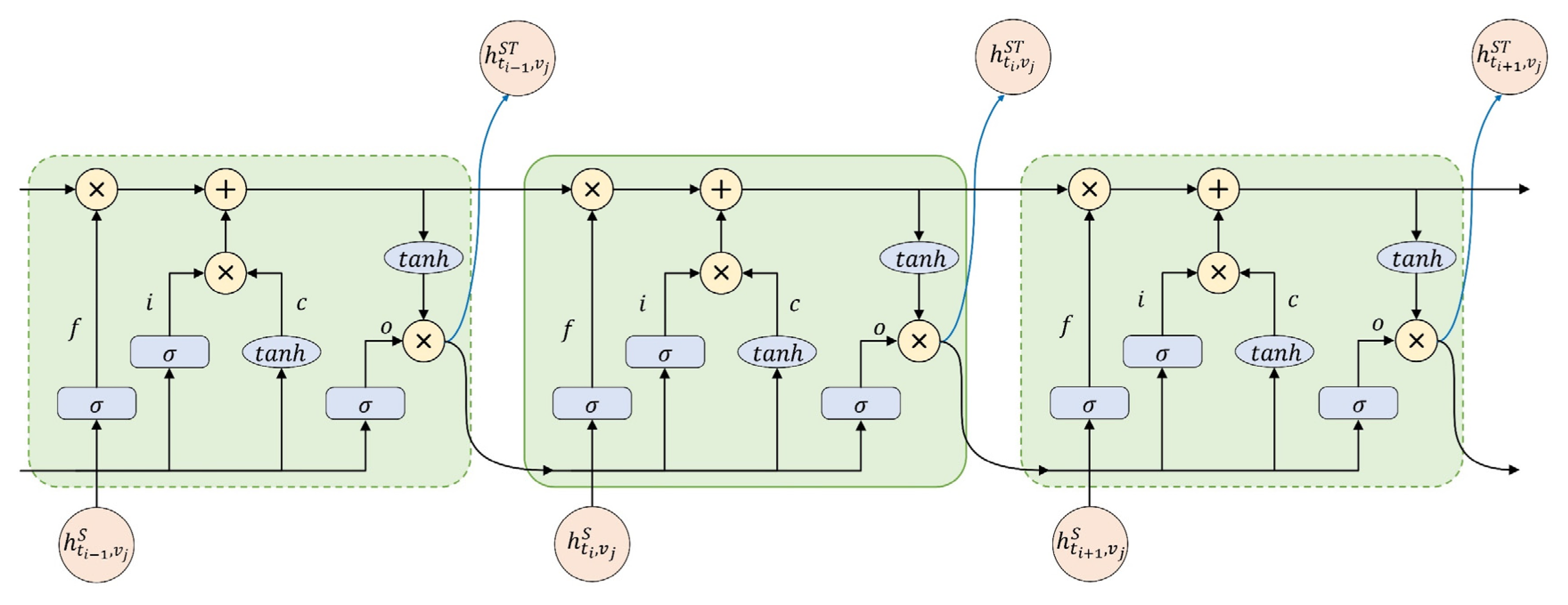
Temporal correlation is one of the important features of air quality data. Previous studies have mainly studied it from the temporal dimension. LSTM is the mainstream method for temporal feature extraction. This paper uses it as a temporal feature extractor. Multi-layer LSTM is used to capture the temporal correlation of air quality data [55]. Figure 6 depicts the temporal feature extractor’s operation.

Figure 6. LSTM architecture.

For node $v_j$, the output of the spatial feature extractor is $h_{t_i{,v}_j}^S$, and LSTM is used to extract its temporal features. Assume that i, f, o represent the input gate, forget gate, and output gate, respectively, $h_{t_i{,v}_j}^S$ is the input of each time step $t_i$, and $h_{t_i{,v}_j}^{ST}$ is the output of each time step $t_i$. σ represents the sigmoid function, tanℎ represents the Tanh function. The extraction process of temporal correlation is shown in the following equation:

Step 1: LSTM selectively forgets the feature information of the cell state $c_{t_{i-1}{,v}_j}$ at time step $t_i$:

$$f_{t_i{,v}_j}=\sigma \left(W_f·\left[h_{t_{i-1}{,v}_j}^{ST},h_{t_i{,v}_j}^S\right]\right)+b_f$$

(8)

$$c_{t_i{,v}_j}^{\prime }=f_{t_i{,v}_j}\circ c_{t_{i-1}{,v}_j}$$

(9)

Step 2: LSTM extracts important information from the input features to update the state unit $c_{t_i{,v}_j}^{\prime }$:

$$i_{t_i{,v}_j}=\sigma \left(W_i·\left[h_{t_{i-1}{,v}_j}^{ST},h_{t_i{,v}_j}^S\right]\right)+b_i$$

(10)

$${\tilde{c}}_{t_i{,v}_j}=tanh\left(W_c·\left[h_{t_{i-1}{,v}_j}^{ST},h_{t_i{,v}_j}^S\right]\right)+b_c$$

(11)

$$c_{t_i{,v}_j}=c_{t_i{,v}_j}^{\prime }+i_{t_i{,v}_j}\circ {\tilde{c}}_{t_i{,v}_j}$$

(12)

Step 3: Finalize the LSTM output:

$$o_{t_i{,v}_j}=\sigma \left(W_o·\left[h_{t_{i-1}{,v}_j}^{ST},h_{t_i{,v}_j}^S\right]\right)+b_o$$

(13)

$$h_{t_i{,v}_j}^{ST}=o_{t_i{,v}_j}\circ tanh\left(v_{t_i{,v}_j}\right)$$

(14)

The entire GLSTM-Block workflow described above introduces the extraction process of the spatiotemporal features $h_{t_i}$ of air quality data at time step $t_i$, including dynamic spatial features and temporal features.

3.5. Temporal Self-Attention Module in Decoder

The spatial attention in GAT and temporal attention in the decoding unit serve distinct, complementary roles. GAT’s spatial attention identifies which neighboring monitoring stations are most relevant at each time step (capturing “where” pollutants disperse across the network), while temporal attention identifies which historical time steps are most informative for future predictions (capturing “when” historical patterns matter). These two mechanisms operate on orthogonal dimensions—spatial and temporal—and both are necessary to capture the full spatiotemporal dependencies in air quality data.

For node $v_j$ and spatiotemporal feature $\widehat{h}$, the temporal correlation can be calculated through the multi-head attention mechanism. The influence weight ${\beta }_{t_{n+i},t}$ of all time steps from $t_1$ to $t_{n+i}$ on the time step $t_{n+r}$ is calculated through the multi-head self-attention mechanism, as shown in the following formula:

$${\beta }_{t_{n+i},t}={\displaystyle \frac{exp\left(u_{t_{n+i},t}\right)}{exp\left({\sum }_{t_r}^{z_{t_{n+i}}}{u}_{t_{n+i},t_r}\right)}}$$

(15)

where $z_{t_{n+i}}$ is a set of time steps before $t_{n+i}$, $u_{t_{n+i},t}$ represents the correlation between the temporal features of time steps $t_{n+i}$ and $t$, which can be obtained by the inner product of the query vector of node $v_j$ at time step $t_{n+i}$ and the key vector of node $v_j$ and time step $t$, as shown in the following equation:

$$u_{t_{n+i},t}={\displaystyle \frac{f_k^q\left(\left({\widehat{h}}_{t_{n+i},v_j}+e_t^{t_{n+i},v_j}\right)W_k^q\right)·f_k^k\left(\left({\widehat{h}}_{t_{n+i},v_j}+e_t^{{t,v}_j}\right)W_k^k\right)}{\sqrt{d}}}$$

(16)

After obtaining the impact ${\beta }_{t_{n+i},t}$, the hidden state ${\breve{h}}_{t_{n+i},v_j}^k$ is updated by Equation (16).

$${\breve{h}}_{t_{n+i},v_j}^k={\sum }_{t_r}^{z_{t_{n+i}}}{\beta }_{t_{n+i},t_r}^k{V}_{t_r}^k+{\widehat{h}}_{t_{n+i},v_j}$$

(17)

$$V_{t_r}^k=f_k^v\left(\left({\widehat{h}}_{t_r,v_j}+e_t^{{t_r,v}_j}\right)W_k^v\right)$$

(18)

The temporal relevance of $v_j$ is obtained by multiplying the influence weight ${\beta }_{t_{n+i},t}$ and $V^k{=V}_t^k|t\in z_{t_{n+i}}$, and the multi-head self-attention mechanism is adopted.

$$h_{t_{n+i}}^{″}=\left[{\breve{h}}_{t_{n+i},v_j}^1,\cdots ,{\breve{h}}_{t_{n+i},v_j}^M\right]W^o$$

(19)

At time step $t_{n+i}$, the temporal correlation can be calculated using Equations (15)–(19) above, and the AQI output is $h_{t_{n+i}}^{″}$. To generate the expected value for the AQI prediction task, the fully connected layer directly receives the decoder’s output features.

Finally, the GLA-Net model suggested in this paper is contrasted with alternative prediction models. Metrics like RMSE, MAE, and IA are employed to verify the efficacy of the suggested approach [16].

4. Result

4.1. Parameter Setting

Through extensive experimentation, we established a uniform 64-dimensional representation across all network components (GAT QKV projections, LSTM hidden states, temporal attention QKV, and dense connection layers). This design emerged from systematic optimization addressing both model performance and overfitting concerns. First, comparative experiments with alternative dimensions (32, 64, 128, 256) revealed that 64-dim achieves optimal balance. Lower dimensions (32) provided insufficient representational capacity, causing RMSE degradation. Higher dimensions (128, 256) increased parameters by 4–16 times without proportional performance gains, introducing overfitting particularly in smaller datasets. Second, dimensional consistency across modules yields critical architectural benefits. When GAT spatial features, LSTM temporal representations, and attention mechanisms share 64-dim, the model eliminates dimension transformation layers between components. This simplifies architecture, reduces parameters, and enables seamless information flow. The additive fusion and attention computations proceed efficiently without dimensional mismatches requiring additional projections. Third, maintaining 64-dim in dense connection layers preserves feature fidelity across network depth.

Specifically, as shown in Table 2, optimal hyperparameter selection was achieved through systematic iterative experimentation. The dataset underwent fixed partitioning: 70% allocated to model training, 15% to validation, and 15% to testing. This stratification strategy differs from k-fold cross-validation by preserving temporal sequence integrity, thereby preventing information leakage inherent in time-series forecasting tasks. Real-time model evaluation occurred during training via the validation subset. Following each iteration, we computed root mean square error (RMSE) and mean absolute error (MAE) metrics to assess predictive accuracy. Parameter configurations yielding superior performance were dynamically saved and updated throughout the optimization cycle. The training regimen encompassed 100 epochs, with validation-based assessment conducted after each complete pass through the training data. When validation metrics (RMSE, MAE) demonstrated improvement, the corresponding network weights were preserved. To mitigate overfitting risks, we implemented a 0.5 dropout probability informed by preliminary experimental trials. Batch size (32 samples) and learning rate (0.001) emerged from grid search exploration, aligning with established practices in spatiotemporal forecasting literature. Additionally, an early termination mechanism monitored validation performance to guarantee convergence stability and prevent unnecessary computational expenditure.

Table 2. GLA-Net model parameter.

Layer Name	Parameters	Values
GAT	$q$: [layer nodes] × number of layers	64 × 1
	$k$: Same as above	64 × 1
	$v$: Same as above	64 × 1
	number of heads	4
LSTM	[layer nodes] × number of layers	64 × 1
Temporal attention	$q$: [layer nodes] × number of layers	64 × 1
	$k$: Same as above	64 × 1
	$v$: Same as above	64 × 1
	number of heads	4
Dense connected layer	[layer nodes] × number of layers	64 × 1
Fully connected layer	Same as above	256 × 1
	Same as above	1 × 1
-	Dropout	0.5
-	Batch size	32
-	Learning rate	0.0001
-	Epochs	100
-	Training method	Adam

4.2. One-Step Forecasting

In the one-step prediction experiment, we use the historical data of three consecutive hours to predict the AQI of the next hour. Specifically, the model can predict the AQI at 13:00 based on the pollutant concentration and meteorological records from 10:00 to 12:00.

4.2.1. Baseline Model

To evaluate the performance and advantages of the proposed model, we compare it with the following state-of-the-art machine learning and deep learning models in air pollutant concentration prediction tasks.

(1)

SVM (Support Vector Machine): Support Vector Machine is a classic machine learning algorithm that finds the optimal hyperplane to separate different classes. It has been widely applied in air quality classification and pattern recognition tasks.

(2)

SVR (Support Vector Regression): Support Vector Regression is the regression variant of SVM, which uses the same principles to predict continuous values. It is commonly used as a baseline model in air pollutant concentration forecasting due to its robustness to outliers.

(3)

XGBoost (Extreme Gradient Boosting): Extreme Gradient Boosting is an advanced ensemble learning algorithm based on gradient boosting decision trees. It has become one of the most popular machine learning models in air quality prediction tasks due to its high accuracy and efficiency.

(4)

CatBoost (Categorical Boosting): Categorical Boosting is a gradient boosting algorithm that excels at handling categorical features. This model is selected for comparison to demonstrate the performance of advanced ensemble methods in air pollutant concentration prediction.

(5)

CNN (Convolutional Neural Network): Convolutional neural network is one of the most classic deep learning models in air pollutant concentration prediction tasks. It effectively captures spatial features and local patterns in sequential data.

(6)

LSTM (Long Short-Term Memory): Long Short-Term Memory is a recurrent neural network architecture designed to capture long-term temporal dependencies. It is widely used as a baseline model for time series prediction in air quality forecasting.

(7)

CNN-LSTM: Combine CNN with LSTM to build a hybrid deep learning model. This model leverages CNN for spatial feature extraction and LSTM for temporal dependency modeling, demonstrating the advantages of the hybrid architecture.

(8)

ResNet-LSTM: Combine Residual Network with LSTM to build a hybrid deep learning model. This architecture uses ResNet’s skip connections to extract deep features while LSTM captures temporal patterns, addressing the degradation problem in deep networks.

(9)

GCN-LSTM: Combine Graph Convolutional Network with LSTM to build a hybrid deep learning model. This model captures spatial correlations between monitoring stations through GCN and temporal dependencies through LSTM, suitable for multi-site air quality prediction.

(10)

GLSTM-Block: This model is based on Section 3.4 of the article.

(11)

GLSTM-Block-LSTM: This model is GLA-Net without added temporal attention.

All baseline models were trained and tested using the same dataset, hyperparameters, and evaluation metrics as the proposed model to ensure a fair and comprehensive comparison.

4.2.2. Comparison of Methods

Table 3 shows the prediction performance of GLA-Net and the comparison model for 1 h AQI on the test set, covering indicators such as RMSE, MAE and IA. The results show that compared with traditional machine learning methods and single classical neural networks, CNN and LSTM perform better in prediction. Among the hybrid deep learning models, CNN-LSTM, ResNet-LSTM, GCN-LSTM and GLA-Net all show stronger AQI fitting ability, indicating that these models have more advantages in dealing with time series problems with spatial characteristics. Further analysis shows that the prediction accuracy of ResNet-LSTM is better than that of CNN-LSTM, indicating that ResNet is more effective in extracting spatial features of pollutants and meteorological data. The prediction accuracy of GCN-LSTM is higher than that of ResNet-LSTM, indicating that GCN can better capture spatiotemporal dependencies, thereby improving the prediction ability of the model. Finally, compared to GCN-LSTM, GLA-Net improved the average prediction performance by 6.78%, demonstrating its superiority in extracting spatiotemporal features from time series data. However, referring to the performance in the three datasets and comparing with CNN-LSTM, ResNet-LSTM and GCN-LSTM, the performance improvement of GLA-Net is limited. This may be because the single-step prediction task itself is relatively easy, resulting in relatively unobvious effects of model improvement.

Table 3. Single-step prediction.

Model	Beijing (1006A Station)			Shanghai (1147A Station)			Shenzhen (1358A Station)
	RMSE	MAE	IA	RMSE	MAE	IA	RMSE	MAE	IA
SVM	24.174	18.547	0.871	17.941	13.394	0.862	9.864	7.048	0.859
SVR	23.245	17.846	0.888	16.941	12.457	0.873	9.325	6.978	0.864
XGBoost	21.178	16.645	0.909	15.855	11.678	0.886	8.545	6.378	0.879
CatBoost	20.204	15.187	0.917	15.075	11.248	0.889	8.081	6.148	0.886
CNN	17.214	13.417	0.943	13.172	9.874	0.918	7.124	5.546	0.911
LSTM	15.873	11.274	0.957	12.571	8.546	0.938	6.845	5.077	0.936
CNN-LSTM	14.819	10.589	0.972	11.236	7.789	0.945	6.285	4.500	0.952
ResNet-LSTM	13.941	9.812	0.977	10.465	7.423	0.951	5.863	4.172	0.963
GCN-LSTM	13.639	9.613	0.978	9.789	7.164	0.959	5.519	4.016	0.966
GLSTM-Block	13.852	9.935	0.978	10.125	7.014	0.952	5.517	4.021	0.967
GLSTM-Block-LSTM	12.936	9.041	0.980	8.984	6.441	0.964	5.248	3.684	0.972
GLA-Net	12.716	8.356	0.983	7.612	5.722	0.976	5.039	3.192	0.975

We designed two ablation architectures, GLSTM-Block and GLSTM-Block-LSTM, to quantify the contribution of the temporal feature extraction component. Single-step forecasts reveal minimal performance divergence between the two baseline architectures. GLSTM-Block-LSTM exhibits marginally superior accuracy compared to GLSTM-Block alone. Two factors explain this modest advantage. First, one-step-ahead prediction tasks present relatively straightforward challenges. Second, the independent LSTM pathway effectively captures temporal dependencies directly from raw input data, reducing reliance on complex features. The complete GLA-Net architecture surpasses both simplified variants across all prediction horizons. This superiority validates the strategic integration of temporal attention mechanisms. While GLSTM-Block-LSTM incorporates basic temporal processing, the additional attention layer in GLA-Net enables dynamic weighting of historical observations, substantially enhancing forecasting capability.

4.2.3. Visualization of Model Prediction Capabilities

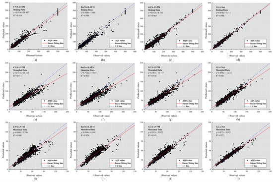
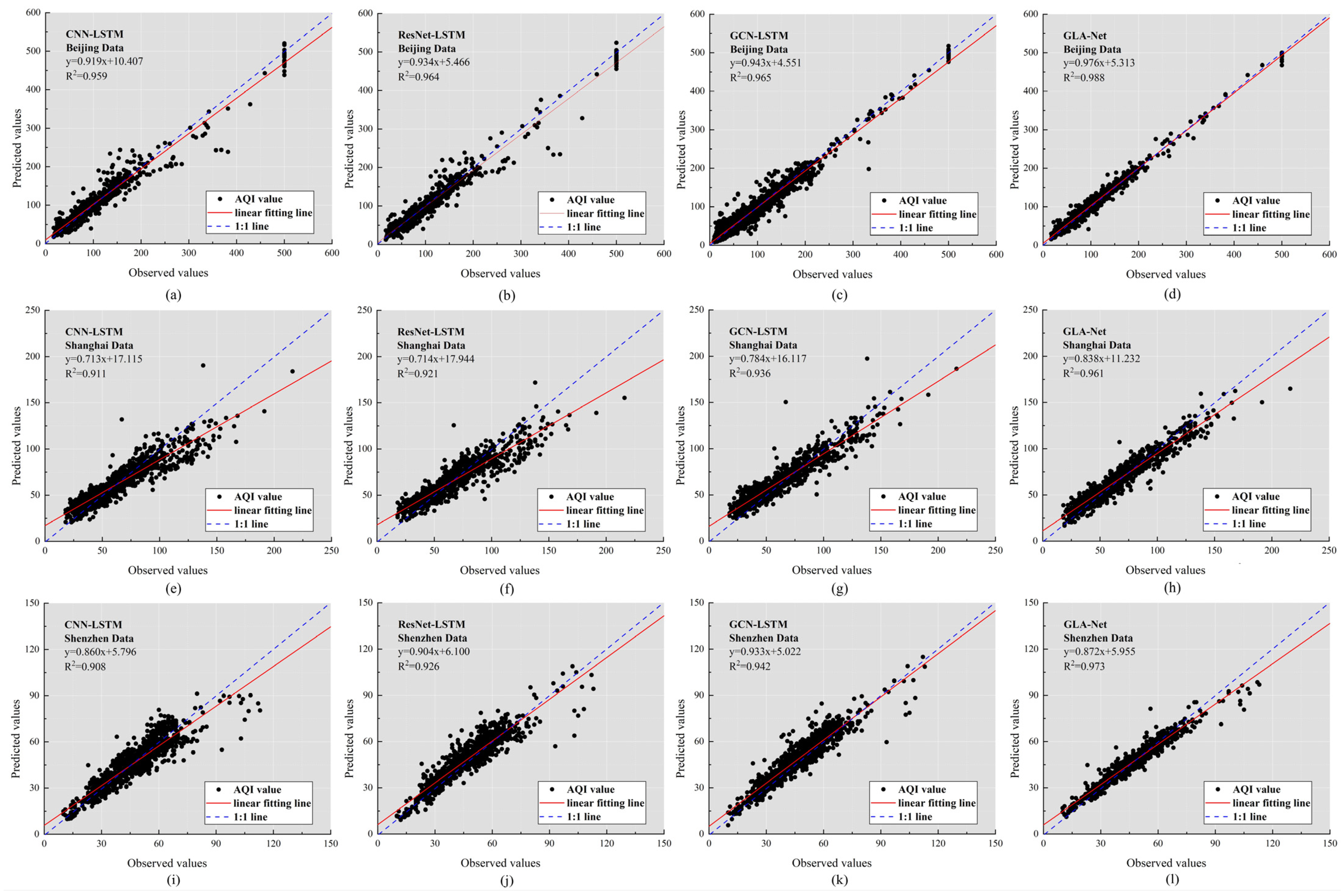
To verify the prediction performance of the GLA-Net model, this study selected four types of cutting-edge models for systematic comparison. As shown in Figure 7, the prediction performance of each model can be intuitively compared through the 1000 h of AQI data randomly selected from the test set in the [1 h-3] task. In the coordinate system setting, the horizontal axis corresponds to the measured AQI value, the vertical axis represents the model prediction value, the blue dotted line corresponds to the y = x reference line, the red solid line is the linear regression result of the measured value and the predicted value, and the black scattered points reflect the degree of deviation between the two. Analysis based on three sets of datasets in Beijing, Shanghai, and Shenzhen shows that when the AQI exceeds 100, the prediction accuracy of each model shows a downward trend. Under this condition, CNN-LSTM presents the largest discreteness, while GLA-Net has the lowest discreteness, indicating that it has the best prediction stability. It is worth noting that even when the AQI is in the range of 0–100, GLA-Net still maintains the lowest discrete distribution. A horizontal comparison of the three datasets shows that the model performs best in Beijing (IA = 0.983), and the prediction accuracy of the Shanghai (IA = 0.976) and Shenzhen (IA = 0.975) datasets is similar and relatively low. Taking the Beijing data as an example, the consistency index (IA) analysis shows that the IA of CNN-LSTM, ResNet-LSTM, GCN-LSTM and GLA-Net are 0.972, 0.977, 0.978 and 0.983, respectively, indicating that GLA-Net achieves the highest degree of prediction consistency. This performance improvement is mainly due to the model architecture’s ability to capture spatiotemporal features in a coordinated manner, but it should be noted that the complexity limitation of the single-step prediction task itself may weaken the significance of the differences between different architectures.

Figure 7. Model prediction performance in single-step prediction. (a–d) Scatter plot of prediction results from CNN-LSTM, ResNet-LSTM, GCN-LSTM, and GLA-Net in the Beijing dataset; (e–h) Scatter plot of prediction results from CNN-LSTM, ResNet-LSTM, GCN-LSTM, and GLA-Net in the Shanghai dataset; (i–l) Scatter plot of prediction results from CNN-LSTM, ResNet-LSTM, GCN-LSTM, and GLA-Net in the Shenzhen dataset.

4.3. Multi-Step Prediction

Usually, the prediction research of AQI is limited to the single-step prediction model, which is difficult to meet the needs of practical applications. Therefore, it is of great significance to carry out multi-period air quality prediction research.

4.3.1. The Predicting Performance of the Suggested Model

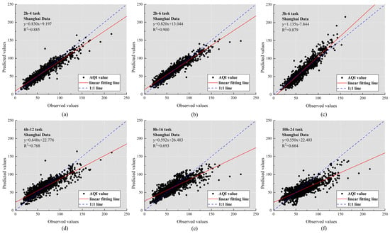
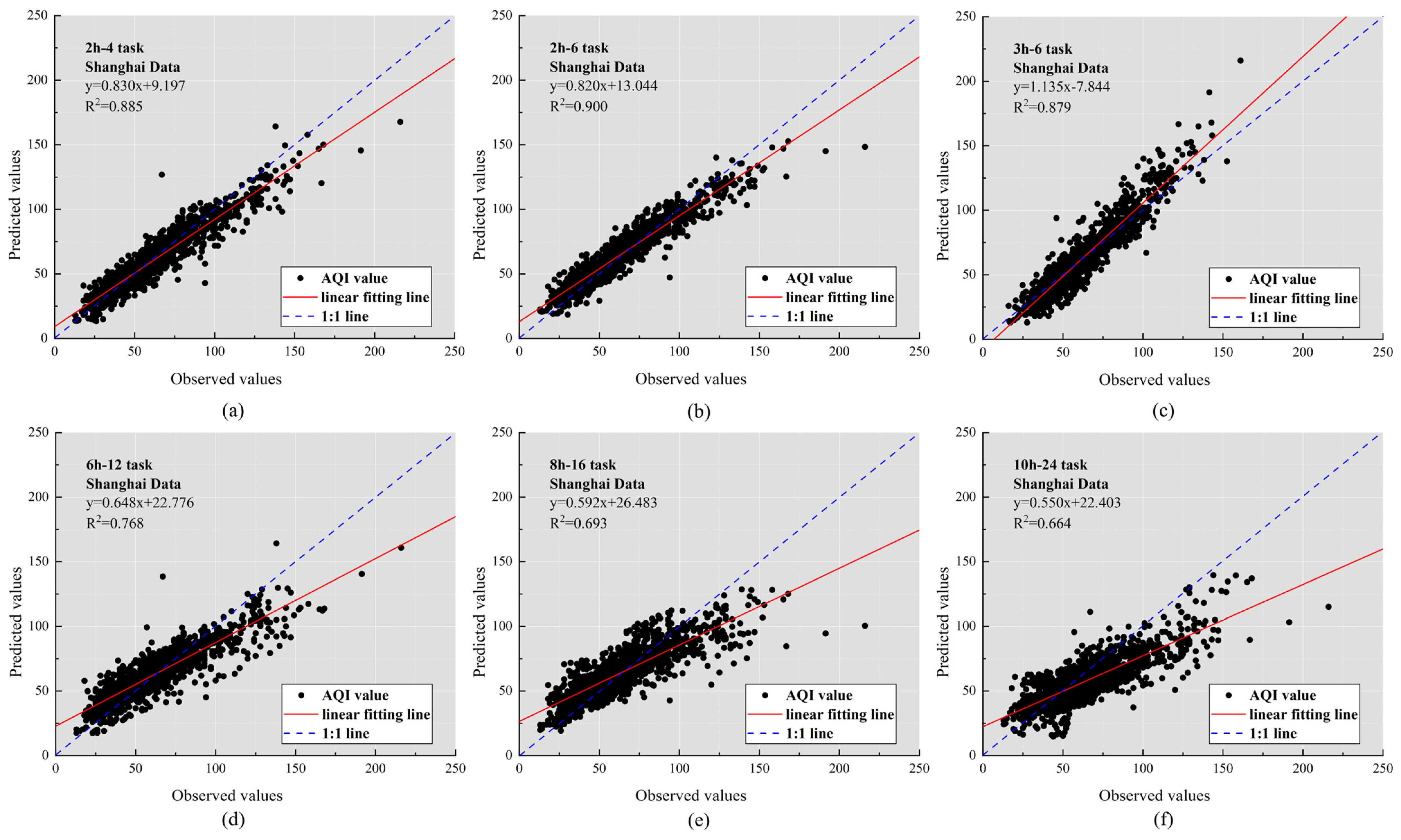
Taking the Shanghai dataset as an example, this study conducts a systematic analysis on six multi-step prediction scenarios (2 h-4, 2 h-6, 3 h-6, 6 h-12, 8 h-16 and 10 h-24), and predicts the AQI value of each time period by building independent models. As shown in Figure 8 and Table 4, the GLA-Net model with a fixed architecture shows a gradual performance degradation law in cross-time prediction: when the prediction time is extended from 2 h to 24 h, the RMSE of the model increases from 10.543 to 23.413, revealing that the prediction error is related to time. The time span is significantly positively correlated. It is worth noting that the optimal selection of the historical data time window has a dual impact on the prediction performance. In the 2 h prediction task, extending the input sequence length r from 4 h to 6 h can improve the model performance, specifically reducing RMSE by 0.276 and MAE by 0.134, while IA and R² increase by 0.001 and 0.005, respectively. Such performance improvements are too minor. However, this accuracy gain comes at the cost of increased computational overhead. Through systematic parameter optimization experiments, this study finally determined the optimal historical data length for each prediction task, achieving a balance between prediction accuracy and computational efficiency.

Figure 8. Model prediction performance in multi-step prediction. (a–f) Scatter plot of prediction results for task 2 h-4, 2 h-6, 3 h-6, 6 h-12, 8 h-16 and 10 h-24.

Table 4. Multi-step prediction in Shanghai dataset.

Task	Historical Time Period	RMSE	MAE	IA	R2
1–2 h prediction	4 h	10.543	7.712	0.954	0.885
1–2 h prediction	6 h	10.267	7.578	0.955	0.900
1–3 h prediction	6 h	12.696	9.043	0.928	0.879
1–6 h prediction	12 h	19.481	14.267	0.811	0.768
1–8 h prediction	16 h	21.270	15.442	0.754	0.693
1–10 h prediction	24 h	23.413	16.718	0.713	0.664

4.3.2. Model Comparison

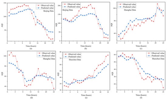
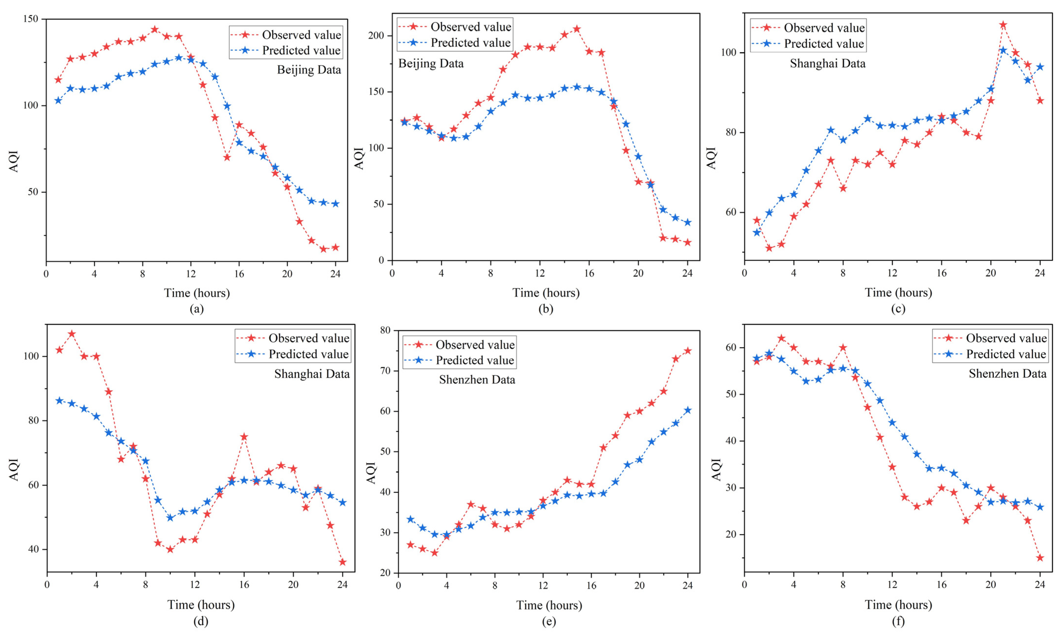
To systematically evaluate generalization ability of proposed model, this study designed a time-based prediction comparison experiment. Using multi-city pollution and meteorological data with a historical span of 24 h as input, two prediction intervals of 1–12 h (short-term) and 13–24 h (medium- and long-term) were constructed. By comparing the prediction performance of GLA-Net with the frontier models (CNN-LSTM, ResNet-LSTM, GCN-LSTM), the data in Table 5 show that in the AQI prediction tasks of the three cities, the RMSE of GLA-Net is the lowest, which shows that in multi-step prediction, the model structure of GLA-Net is suitable for long-term data prediction. To further reveal the temporal adaptation characteristics of the model, Figure 9 shows the dynamic coupling relationship between the measured value and the predicted value of AQI in the continuous prediction of 1–24 h. The random sample analysis based on the test sets of Beijing, Shanghai and Shenzhen shows that GLA-Net accurately grasps the dynamic change law of AQI.

Table 5. Prediction of AQI throughout time.

Model	Beijing (1006A Station)		Shanghai (1147A Station)		Shenzhen (1358A Station)
	1–12 h	13–24 h	1–12 h	13–24 h	1–12 h	13–24 h
CNN-LSTM	25.285	39.429	18.307	26.552	10.534	16.622
ResNet-LSTM	24.005	38.525	16.875	24.960	10.189	14.913
GCN-LSTM	23.578	36.079	16.428	24.071	9.806	14.743
GLA-Net	21.011	33.009	14.969	23.568	9.161	14.235

Figure 9. Model prediction performance visualization in 24 h task prediction. (a,b) Line chart of GLA-Net’s multi-step prediction results in the Beijing dataset; (c,d) Line chart of GLA-Net’s multi-step prediction results in the Shanghai dataset; (e,f) Line chart of GLA-Net’s multi-step prediction results in the Shenzhen dataset.

4.3.3. Analysis of the Error Distribution

This section examines prediction error patterns using a two-hour-ahead AQI forecasting model applied to the complete dataset. Error distributions are analyzed across three dimensions: pollutant concentration levels, geographic locations, and temporal periods. Table 6 presents six AQI grades. Temporal analysis follows natural seasonal cycles: spring encompasses March through May, summer spans June to August, autumn covers September to November, and winter includes December through February.

Table 6. Predicted AQI concentration for different ranges.

AQI	Beijing (1006A Station)		Shanghai (1147A Station)		Shenzhen (1358A Station)
	Percentage	RMSE	Percentage	RMSE	Percentage	RMSE
$0<x\le 50$	47.55%	9.36	54.71%	6.98	78.39%	3.35
$50<x\le 100$	36.75%	10.64	40.26%	7.60	20.49%	3.81
$100<x\le 150$	8.29%	17.58	4.42%	12.73	0.99%	15.83
$150<x\le 200$	4.26%	19.65	0.27%	23.01	0.06%	42.14
$200<x\le 300$	2.35%	39.71	0.13%	41.09	0.07%	67.68
$>300$	0.80%	70.91	0.21%	62.82	-	-

After controlling for sample size variations, Table 6 reveals three notable patterns. First, air quality distribution differs substantially among cities. Shenzhen demonstrates superior environmental conditions, with 78.39% of observations falling below AQI 50 (excellent quality), compared to Beijing’s 47.55% and Shanghai’s 54.71%. Second, prediction accuracy varies inversely with pollution severity. At low concentration levels (AQI 0–50), the model achieves strong performance with RMSE values of 9.36 (Beijing), 6.98 (Shanghai), and 3.35 (Shenzhen). Shenzhen’s model exhibits particularly robust accuracy in this range. Third, forecast errors increase markedly as pollution intensifies, with degradation becoming pronounced at elevated AQI levels.

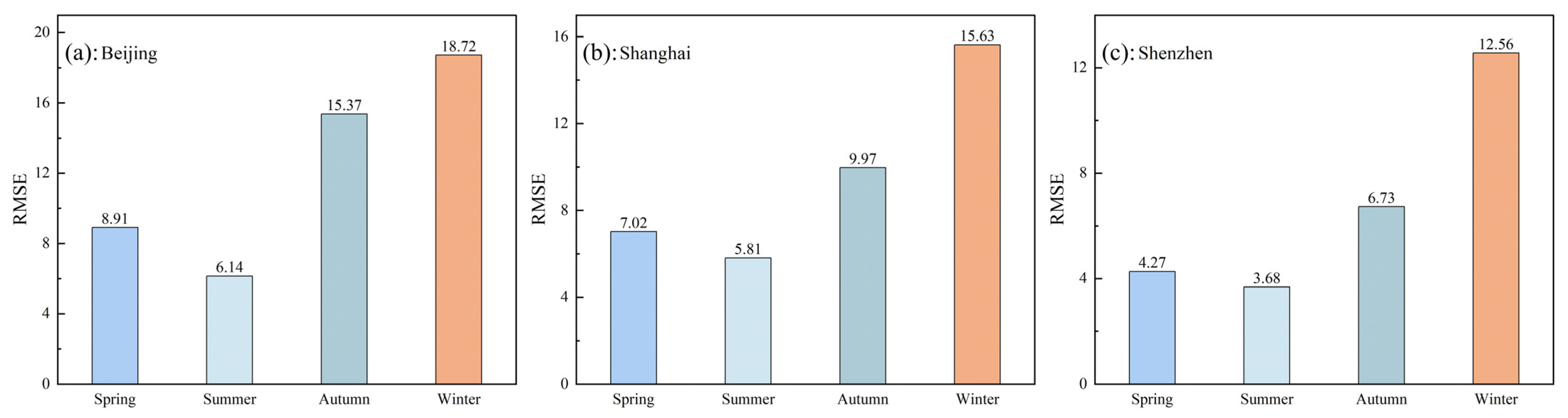
Seasonal analysis presented in Figure 10 demonstrates two key findings. The model exhibits clear temporal performance variations across all three cities, achieving lowest errors during summer months and highest errors in winter. This pattern remains consistent regardless of location. This seasonal variation can be attributed to several meteorological and atmospheric factors. During summer, air pollutant dispersion is enhanced by higher temperatures, stronger convection, and more stable weather patterns, leading to more predictable pollution dynamics. In contrast, winter is characterized by frequent temperature inversions, complex atmospheric boundary layer structures, and heating-related emission increases, which create more challenging forecasting conditions. The higher RMSE values in winter (Beijing: 18.72, Shanghai: 15.63, Shenzhen: 12.56) reflect these complexities, where the model encounters greater difficulty in capturing rapid pollution accumulation events and dispersion processes.

Figure 10. Model prediction performance visualization in 24 h task prediction. (a) A bar chart of GLA-Net’s seasonal prediction results in the Beijing dataset; (b) A bar chart of GLA-Net’s seasonal prediction results in the Shanghai dataset; (c) A bar chart of GLA-Net’s seasonal prediction results in the Shenzhen dataset.

Additionally, Shenzhen maintains superior prediction quality throughout the annual cycle, with optimal performance occurring in summer (RMSE = 3.68) and spring (RMSE = 4.27). These results reflect both the region’s relatively stable atmospheric conditions and the model’s enhanced capability in forecasting moderate pollution scenarios. Specifically, Shenzhen’s coastal location and subtropical climate contribute to more uniform meteorological conditions with less extreme seasonal variations compared to Beijing and Shanghai. The city experiences fewer severe pollution episodes and more consistent wind patterns that facilitate pollutant dispersion. Furthermore, the absence of winter heating-related emissions in Shenzhen reduces the seasonal volatility in pollution levels, resulting in a narrower RMSE range (3.68–12.56) across seasons compared to Beijing (8.91–18.72) and Shanghai (7.02–15.63). This demonstrates that the model performs more reliably in environments with moderate pollution levels and stable atmospheric dynamics, while it faces greater challenges in regions with high pollution variability and complex seasonal emission patterns.

4.4. Prediction of PM_2.5 Concentration

To evaluate the versatility and migration ability of the model, we extended GLA-Net to the 24 h PM_2.5 prediction task. The experiment compared the performance of cutting-edge models such as CNN-LSTM, ResNet-LSTM, and GCN-LSTM. As shown in Table 7. GLA-Net achieved the lowest RMSE in the prediction of each time period, showing excellent prediction accuracy. These results not only verify the excellent performance of the model in PM_2.5 prediction, but also confirm its practical value as a general air pollutant prediction tool.

Table 7. PM_2.5 concentration prediction in 24 h task.

Model	Beijing (1006A Station)		Shanghai (1147A Station)		Shenzhen (1358A Station)
	RMSE (µg/m3)	IA	RMSE (µg/m3)	IA	RMSE (µg/m3)	IA
CNN-LSTM	31.980	0.767	23.723	0.659	13.879	0.641
ResNet-LSTM	30.456	0.781	22.664	0.670	13.247	0.652
GCN-LSTM	30.312	0.783	22.194	0.673	12.883	0.659
GLA-Net	29.014	0.791	21.317	0.684	11.764	0.667

5. Discussion

5.1. In Contrast to Earlier Prediction Models

The experimental results of single-step prediction reveal the significant advantages of deep learning models in the field of air quality prediction. From the perspective of architecture evolution, the performance improvement of ResNet-LSTM over CNN-LSTM can be attributed to the introduction of residual connections, which effectively alleviates the gradient vanishing problem of deep networks, thereby enhancing the ability to capture pollutant diffusion patterns. Further improvements to GCN-LSTM reflect the unique advantages of graph structures in describing spatial dependencies, which is highly consistent with the transmission characteristics of air pollutants. GLA-Net has made breakthroughs in the collaborative modeling of spatiotemporal features by integrating the attention mechanism.

As can be seen from Table 3, the experimental results reveal significant regional differences. The Beijing dataset exhibits the highest prediction IA (0.983), but also the largest RMSE (12.716). This performance characteristic is associated with the higher mean AQI value (64.289) and significant concentration fluctuations in the region. Although the model accurately grasps the changing trend of Beijing’s air quality, the large fluctuations in pollutant concentrations lead to an increase in the absolute error of the prediction. In contrast, the prediction performances of Shanghai (IA = 0.976, mean AQI 48.656) and Shenzhen (IA = 0.975, mean AQI 36.554) are different. Shenzhen, in particular, achieved the lowest RMSE (5.039) due to its low overall pollution level and small fluctuations, but the relatively low IA reflects the limitations of the model in capturing small fluctuations.

Further analysis of Figure 7 reveals a critical limitation: the model exhibits significant prediction degradation at high pollution levels (AQI > 100). This performance decline can be attributed to several factors. First, high pollution episodes are relatively rare in the training data (accounting for only 15.67% of samples in Beijing, 5.03% in Shanghai, and 1.12% in Shenzhen), resulting in insufficient learning of extreme pollution patterns. The class imbalance causes the model to be optimized primarily for moderate pollution conditions (AQI < 100), which dominate the training distribution. Second, high pollution events often involve complex nonlinear dynamics, including sudden emission surges, stagnant meteorological conditions, and regional pollutant transport, which are difficult to capture with limited historical data. Third, the attention mechanisms, while effective at identifying relevant spatial and temporal patterns under normal conditions, may struggle to properly weight features during atypical high pollution scenarios that differ substantially from training examples.

The RMSE-IA trade-off observed across regions reflects the model’s varying applicability to different pollution regimes. For Beijing, the high IA (0.983) indicates that GLA-Net successfully captures the overall temporal trend and pollution dynamics, but the large RMSE (12.716) suggests systematic underprediction during severe pollution episodes and overprediction during clean periods. This implies that while the model is applicable for general air quality monitoring and moderate pollution forecasting, it requires caution when used for high pollution early warning systems. For cities with stable, low pollution levels like Shenzhen, the model achieves high accuracy (RMSE = 5.039) but may lack sensitivity to subtle variations, as indicated by the slightly lower IA. This suggests the model is most reliable for regions with moderate pollution variability and may require enhancement for both extreme pollution scenarios and low-variability environments.

To improve applicability across all pollution regimes, future work should consider: (1) implementing pollution-level-specific loss functions or weighted sampling to address class imbalance; (2) incorporating auxiliary features such as emission inventories and synoptic weather patterns that are particularly informative during high pollution events; (3) developing ensemble approaches that combine GLA-Net with physics-based models for extreme pollution forecasting; and (4) augmenting training data with synthetic high pollution scenarios based on atmospheric dispersion principles.

5.2. Predicting Long-Term Series and Comparing Models

The research team trained the GLA-Net model for multi-step predictions for different time windows of 1–10 h. The experiment found that as the prediction time span increases, the prediction accuracy shows a downward trend. Taking the 2 h prediction as an example, although increasing the amount of historical data can improve the accuracy, after weighing the computational overhead, we determined the optimal historical data input length for each prediction task.

The comparison results in Table 5 show that the average prediction error of GLA-Net at all time scales is lower than that of benchmark models such as CNN-LSTM, ResNet-LSTM and GCN-LSTM. In order to further evaluate its long-term prediction ability, we randomly selected two groups of samples from the test set of three datasets to analyze the 24 h prediction effect. As shown in Figure 9, the prediction curve (red) and the measured curve (blue) show a highly consistent change pattern. The experiment confirmed the outstanding advantages of GLA-Net in predicting high-concentration pollutants and grasping long-term trends, highlighting its application potential in the field of environmental monitoring.

This study conducts an in-depth examination of forecast deviation patterns across three major Chinese cities. Following national air quality standards, we stratified pollutant concentrations into six hierarchical categories and organized temporal data by seasonal periods. The analysis encompassed Beijing, Shanghai, and Shenzhen, revealing distinct regional performance disparities. Shenzhen demonstrated superior outcomes across multiple evaluation dimensions. The city exhibited exceptional environmental quality, with 78.39% of observations falling within minimal pollution thresholds. Forecast accuracy remained consistently robust, particularly during spring and summer months when the model achieved its lowest error margins. These findings contrast sharply with patterns observed in Beijing and Shanghai, where atmospheric conditions display greater volatility. Winter forecasts in these two metropolitan areas exhibited deviations 3–5 times higher than summer estimates, reflecting pronounced seasonal variability.

These results illuminate substantial inter-city differences in atmospheric dynamics and provide critical insights for refining predictive algorithms. The marked performance variation between stable coastal environments (Shenzhen) and seasonally fluctuating inland regions (Beijing, Shanghai) suggests that location-specific model calibration may enhance forecasting reliability across diverse pollution regimes.

5.3. Utility Analysis of the Model

Our experimental results highlight the excellent performance of the proposed GLA-Net model in the 24 h PM_2.5 forecasting task. By comparing GLA-Net with several baseline models such as CNN-LSTM, ResNet-LSTM, and GCN-LSTM, we demonstrate its superior accuracy in terms of RMSE across all time intervals. These findings not only highlight the effectiveness of the model in predicting PM_2.5 concentrations, but also its versatility and robustness in various air pollution forecasting tasks.

6. Limitations and Future Research Directions

6.1. Limitations

While GLA-Net demonstrates superior performance in AQI prediction by deeply mining the coupling relationship between pollutants and meteorological parameters and establishing a robust spatiotemporal correlation modeling framework, several limitations warrant acknowledgment:

(1) Graph Construction Limitations: Uniform Threshold Across Heterogeneous Networks: Our average-distance threshold approach fails to adapt to varying station densities across regions. In densely monitored urban areas, this creates overly connected graphs with spatial redundancy, while in sparse rural regions, it may result in isolated nodes missing important connections. This uniform treatment does not account for the order-of-magnitude variation in station density between urban and rural areas.

Static Graph Structure: The current graph topology is fixed based solely on geographic proximity, unable to adapt to dynamic pollutant dispersion patterns influenced by time-varying meteorological conditions (wind, atmospheric stability), topography, and emission sources. More sophisticated approaches could incorporate: (a) adaptive thresholds based on local station density; (b) meteorological features in graph construction; (c) data-driven correlation measures; or (d) fully learnable graph structures.

(2) Limited Cross-Regional Modeling: This study has not yet integrated multi-city geographical correlation characteristics affecting long-range pollutant migration. Our current single-region graph structure may miss important inter-city connections where upwind urban pollution affects downwind regions, limiting cross-regional collaborative prediction accuracy during regional pollution episodes.

6.2. Future Research Directions

To address these limitations, our research team plans to: (1) develop adaptive graph construction methods accounting for regional heterogeneity and meteorological factors; (2) explore dynamic, learnable graph structures; (3) introduce geospatial encoding techniques for multi-city topology networks; and (4) integrate physics-informed constraints from atmospheric dispersion models. These enhancements aim to improve both local and cross-regional forecasting capabilities.

7. Conclusions

Based on the integration of deep learning methods and big data association analysis principles, this study constructs a new prediction framework GLA-Net, which is based on GCN and LSTM and incorporates a temporal attention mechanism. The core function of this model is to capture the spatiotemporal correlation characteristics of pollutant concentrations at multiple sites, thereby achieving accurate prediction of pollution levels in the target area. In terms of feature extraction, a composite module of GLSTM-Block is designed. This module achieves deep mining of dynamic spatiotemporal features by fusing meteorological parameters and pollutant monitoring data from neighboring sites. In order to further enhance the time series modeling capability, a temporal attention mechanism is introduced at the output end of GLSTM-Block. This component can adaptively assign weights to features at different time nodes to capture key time series patterns. In order to optimize the model training process, a dense connection strategy is innovatively adopted in the network architecture, and layer normalization technology is used to effectively alleviate the problems of gradient vanishing and internal covariate shift. Experimental verification shows that the method proposed in this paper exhibits the following advantages in the pollutant concentration prediction task:

(1)

Compared with cutting-edge models such as ResNet-LSTM and GCN-LSTM, this network innovatively integrates GCN, LSTM and temporal attention mechanism, effectively improving the efficiency of capturing the spatiotemporal correlation characteristics of meteorological elements and pollutant data.

(2)

In the prediction tasks in Beijing, Shanghai and Shenzhen, the model showed good AQI trend prediction ability. Especially in Beijing where the pollutant concentration is high, the model’s ability to predict concentration changes has been enhanced, but the prediction error shows a slight amplification phenomenon.

(3)

GLA-Net performed stably in the PM_2.5 concentration experiments in the three cities, proving that the model has wide applicability.

GLA-Net not only solves the long-term dependency problem of traditional time series models by deeply mining the coupling relationship between pollutants and meteorological parameters, but also establishes a robust spatiotemporal correlation modeling framework.

The limitation of this study is that it has not yet integrated the impact of multi-city geographical correlation characteristics on pollutant migration, which may lead to limited cross-regional collaborative prediction accuracy. Therefore, the research team plans to consider introducing geospatial coding technology in subsequent work to enhance the regional collaborative prediction ability of the model by constructing a city topology network diagram.

References

- Sun, X.; Ping, Z.-B.; Dong, Z.-F.; Chen, K.-L.; Zhu, X.-D.; Larry Li, B.; Tan, X.-Y.; Zhu, B.-K.; Liu, X.; Zhou, C.-C.; et al. Resources and environmental costs of China’s rapid economic growth: From the latest theoretic SEEA framework to modeling practice. J. Clean. Prod. 2021, 315, 128126. [Google Scholar] [CrossRef] [Scilit]
- Zhang, Z.; Zhang, S.; Chen, C.; Yuan, J. A systematic survey of air quality prediction based on deep learning. Alex. Eng. J. 2024, 93, 128–141. [Google Scholar] [CrossRef] [Scilit]
- Tan, X.; Han, L.; Zhang, X.; Zhou, W.; Li, W.; Qian, Y. A review of current air quality indexes and improvements under the multi-contaminant air pollution exposure. J. Environ. Manag. 2021, 279, 111681. [Google Scholar] [CrossRef] [Scilit]
- Wang, K.; Yang, T.; Kong, S.; Li, M. Air quality index prediction through TimeGAN data recovery and PSO-optimized VMD-deep learning framework. Appl. Soft Comput. 2025, 170, 112626. [Google Scholar] [CrossRef] [Scilit]
- Liu, X.; Wan, S.; Fang, B.; Li, X. Dynamics analysis of time-delayed nonlinear system with asymmetric stiffness. Chaos Solitons Fractals 2024, 189, 115624. [Google Scholar] [CrossRef] [Scilit]
- Dongre, P.K.; Patel, V.; Bhoi, U.; Maltare, N.N. An outlier detection framework for Air Quality Index prediction using linear and ensemble models. Decis. Anal. J. 2025, 14, 100546. [Google Scholar] [CrossRef] [Scilit]
- Yang, H.; Zhang, Y.; Li, G. Air quality index prediction using a new hybrid model considering multiple influencing factors: A case study in China. Atmos. Pollut. Res. 2023, 14, 101677. [Google Scholar] [CrossRef] [Scilit]
- Li, D.; Liu, J.; Zhao, Y. Prediction of Multi-Site PM2.5 Concentrations in Beijing Using CNN-Bi LSTM with CBAM. Atmosphere 2022, 13, 1719. [Google Scholar] [CrossRef] [Scilit]
- Baklanov, A.; Zhang, Y. Advances in air quality modeling and forecasting. Glob. Transit. 2020, 2, 261–270. [Google Scholar] [CrossRef] [Scilit]
- Gao, Z.; Zhou, X. A review of the CAMx, CMAQ, WRF-Chem and NAQPMS models: Application, evaluation and uncertainty factors. Environ. Pollut. 2024, 343, 123183. [Google Scholar] [CrossRef] [Scilit]
- Ma, X.; Liu, H.; Peng, Z. Improving WRF-Chem PM2.5 predictions by combining data assimilation and deep-learning-based bias correction. Environ. Int. 2025, 195, 109199. [Google Scholar] [CrossRef] [Scilit] [PubMed]
- Li, Q.; Li, J.; Wang, Z.; Liu, B.; Wang, W.; Wang, Z. Development of a city-level surface ozone forecasting system using deep learning techniques and air quality model: Application in eastern China. Atmos. Environ. 2024, 339, 120865. [Google Scholar] [CrossRef] [Scilit]
- Li, D.; Liu, J.; Zhao, Y. Forecasting of PM2.5 Concentration in Beijing Using Hybrid Deep Learning Framework Based on Attention Mechanism. Appl. Sci. 2022, 12, 11155. [Google Scholar] [CrossRef] [Scilit]
- Yan, R.; Liao, J.; Yang, J.; Sun, W.; Nong, M.; Li, F. Multi-hour and multi-site air quality index forecasting in Beijing using CNN, LSTM, CNN-LSTM, and spatiotemporal clustering. Expert Syst. Appl. 2021, 169, 114513. [Google Scholar] [CrossRef] [Scilit]
- Yu, M.; Masrur, A.; Blaszczak-Boxe, C. Predicting hourly PM2.5 concentrations in wildfire-prone areas using a SpatioTemporal Transformer model. Sci. Total Environ. 2023, 860, 160446. [Google Scholar] [CrossRef] [Scilit] [PubMed]
- Li, D.; Wang, J.; Tian, D.; Chen, C.; Xiao, X.; Wang, L.; Wen, Z.; Yang, M.; Zou, G. Residual neural network with spatiotemporal attention integrated with temporal self-attention based on long short-term memory network for air pollutant concentration prediction. Atmos. Environ. 2024, 329, 120531. [Google Scholar] [CrossRef] [Scilit]
- Chen, C.; Wang, J.; Li, D.; Sun, X.; Zhang, J.; Yang, C.; Zhang, B. Unraveling nonlinear effects of environment features on green view index using multiple data sources and explainable machine learning. Sci. Rep. 2024, 14, 30189. [Google Scholar] [CrossRef] [Scilit]
- Zhang, B.; Zou, G.; Qin, D.; Lu, Y.; Jin, Y.; Wang, H. A novel Encoder-Decoder model based on read-first LSTM for air pollutant prediction. Sci. Total Environ. 2021, 765, 144507. [Google Scholar] [CrossRef] [Scilit]
- Yang, J.; Yan, R.; Nong, M.; Liao, J.; Li, F.; Sun, W. PM2.5 concentrations forecasting in Beijing through deep learning with different inputs, model structures and forecast time. Atmos. Pollut. Res. 2021, 12, 101168. [Google Scholar] [CrossRef] [Scilit]
- Zou, G.; Zhang, B.; Yong, R.; Qin, D.; Zhao, Q. FDN-learning: Urban PM2.5-concentration Spatial Correlation Prediction Model Based on Fusion Deep Neural Network. Big Data Res. 2021, 26, 100269. [Google Scholar] [CrossRef] [Scilit]
- Tu, X.-Y.; Zhang, B.; Jin, Y.-P.; Zou, G.-J.; Pan, J.-G.; Li, M.-Z. Longer Time Span Air Pollution Prediction: The Attention and Autoencoder Hybrid Learning Model. Math. Probl. Eng. 2021, 2021, 5515103. [Google Scholar] [CrossRef] [Scilit]
- Zhang, R.; Awang, N. A novel ST-iTransformer model for spatio-temporal ambient air pollution forecasting. J. Big Data 2025, 12, 101. [Google Scholar] [CrossRef] [Scilit]
- Cao, K.; Zhang, T.; Huang, J. Advanced hybrid LSTM-transformer architecture for real-time multi-task prediction in engineering systems. Sci. Rep. 2024, 14, 4890. [Google Scholar] [CrossRef] [Scilit]
- Zhang, Y.; Cheng, W.; Sun, J.; Wang, L.; Fan, S.; Zhang, J.; Jiang, S. An adaptive hybrid MEMD-Transformer-BiGRU model using MPA algorithm for air quality prediction. Swarm Evol. Comput. 2025, 98, 102099. [Google Scholar] [CrossRef] [Scilit]
- Liu, S.; Hu, Y. Air quality prediction based on factor analysis combined with Transformer and CNN-BILSTM-ATTENTION models. Sci. Rep. 2025, 15, 20014. [Google Scholar] [CrossRef] [Scilit]
- Khatibi, V.; Nikpour, P. Advancing multi-pollutant air quality forecasting using Transformer-based Informer architecture. Earth Sci. Inform. 2025, 18, 287. [Google Scholar] [CrossRef] [Scilit]
- Ma, G.; Xu, K.; Zhang, Y.; Zhang, L.; Chen, Z. A novel deep learning model for air quality index prediction integrating time series decomposition and intelligent optimization. Results Eng. 2025, 27, 106078. [Google Scholar] [CrossRef] [Scilit]
- Luo, K.; Liao, S.; Guan, Z.; Liu, B. An enhanced hybrid adaptive physics-informed neural network for forward and inverse PDE problems. Appl. Intell. 2025, 55, 255. [Google Scholar] [CrossRef] [Scilit]
- Zhang, Z.; Wang, Q.; Zhang, Y.; Shen, T.; Zhang, W. Physics-informed neural networks with hybrid Kolmogorov-Arnold network and augmented Lagrangian function for solving partial differential equations. Sci. Rep. 2025, 15, 10523. [Google Scholar] [CrossRef] [Scilit] [PubMed]
- Zhang, X.; Song, Y.; Nam, W.-H.; Huang, T.; Gu, X.; Zeng, J.; Huang, S.; Chen, N.; Yan, Z.; Niyogi, D. Data fusion of satellite imagery and downscaling for generating highly fine-scale precipitation. J. Hydrol. 2024, 631, 130665. [Google Scholar] [CrossRef] [Scilit]
- Moukheiber, D.; Restrepo, D.; Cajas, S.A.; Montoya, M.P.A.; Celi, L.A.; Kuo, K.-T.; López, D.M.; Moukheiber, L.; Moukheiber, M.; Moukheiber, S.; et al. A multimodal framework for extraction and fusion of satellite images and public health data. Sci. Data 2024, 11, 634. [Google Scholar] [CrossRef] [Scilit]
- Zhang, K.; Yang, X.; Cao, H.; Thé, J.; Tan, Z.; Yu, H. Multi-step forecast of PM2.5 and PM10 concentrations using convolutional neural network integrated with spatial–temporal attention and residual learning. Environ. Int. 2023, 171, 107691. [Google Scholar] [CrossRef] [Scilit]
- Zhang, B.; Zou, G.; Qin, D.; Ni, Q.; Mao, H.; Li, M. RCL-Learning: ResNet and convolutional long short-term memory-based spatiotemporal air pollutant concentration prediction model. Expert Syst. Appl. 2022, 207, 118017. [Google Scholar] [CrossRef] [Scilit]
- Qin, D.; Yu, J.; Zou, G.; Yong, R.; Zhao, Q.; Zhang, B. A Novel Combined Prediction Scheme Based on CNN and LSTM for Urban PM2.5 Concentration. IEEE Access 2019, 7, 20050–20059. [Google Scholar] [CrossRef] [Scilit]
- Zeng, Q.; Cao, Y.; Fan, M.; Chen, L.; Zhu, H.; Wang, L.; Li, Y.; Liu, S. Fine particulate matter concentration prediction based on hybrid convolutional network with aggregated local and global spatiotemporal information: A case study in Beijing and Chongqing. Atmos. Environ. 2024, 333, 120647. [Google Scholar] [CrossRef] [Scilit]
- Zou, G.; Lai, Z.; Wang, T.; Liu, Z.; Li, Y. MT-STNet: A Novel Multi-Task Spatiotemporal Network for Highway Traffic Flow Prediction. IEEE Trans. Intell. Transp. Syst. 2024, 25, 8221–8236. [Google Scholar] [CrossRef] [Scilit]
- Zou, G.; Lai, Z.; Ma, C.; Tu, M.; Fan, J.; Li, Y. When Will We Arrive? A Novel Multi-Task Spatio-Temporal Attention Network Based on Individual Preference for Estimating Travel Time. IEEE Trans. Intell. Transp. Syst. 2023, 24, 11438–11452. [Google Scholar] [CrossRef] [Scilit]
- Hu, W.; Zhang, Z.; Zhang, S.; Chen, C.; Yuan, J.; Yao, J.; Zhao, S.; Guo, L. Learning spatiotemporal dependencies using adaptive hierarchical graph convolutional neural network for air quality prediction. J. Clean. Prod. 2024, 459, 142541. [Google Scholar] [CrossRef] [Scilit]
- Shao, Z.; Gao, S.; Zhou, K.; Yang, S. A new multiregional carbon emissions forecasting model based on a multivariable information fusion mechanism and hybrid spatiotemporal graph convolution network. J. Environ. Manag. 2024, 352, 119976. [Google Scholar] [CrossRef] [Scilit] [PubMed]
- Zhao, L.; Song, Y.; Zhang, C.; Liu, Y.; Wang, P.; Lin, T.; Deng, M.; Li, H. T-GCN: A Temporal Graph Convolutional Network for Traffic Prediction. IEEE Trans. Intell. Transp. Syst. 2020, 21, 3848–3858. [Google Scholar] [CrossRef] [Scilit]
- Kuang, Y.; Yuan, S.; Zou, X.; Zhang, J.; Shi, Z.; Zhang, Y.; Meng, F.; Wang, Z. MTDA-STGCN: Modern Temporal and Dual-Attention-Based Spatiotemporal Graph Convolutional Network for 4D Trajectory Prediction. IEEE Trans. Intell. Transp. Syst. 2025; pp. 1–15, early access. [CrossRef] [Scilit]
- Andreoletti, D.; Troia, S.; Musumeci, F.; Giordano, S.; Maier, G.; Tornatore, M. Network Traffic Prediction based on Diffusion Convolutional Recurrent Neural Networks. In Proceedings of the IEEE INFOCOM 2019—IEEE Conference on Computer Communications Workshops (INFOCOM WKSHPS), Paris, France, 29 April–2 May 2019; pp. 246–251. [Google Scholar]
- Ye, J.; Xue, S.; Jiang, A. Attention-based spatio-temporal graph convolutional network considering external factors for multi-step traffic flow prediction. Digit. Commun. Netw. 2022, 8, 343–350. [Google Scholar] [CrossRef] [Scilit]
- Chen, X.; Xia, H.; Wu, M.; Hu, Y.; Wang, Z. Spatiotemporal hierarchical transmit neural network for regional-level air-quality prediction. Knowl.-Based Syst. 2024, 289, 111555. [Google Scholar] [CrossRef] [Scilit]
- Ioffe, S.; Szegedy, C. Batch normalization: Accelerating deep network training by reducing internal covariate shift. In Proceedings of the 32nd International Conference on International Conference on Machine Learning—Volume 37, Lille, France, 7–9 July 2015; pp. 448–456. [Google Scholar]
- Zhang, Z.; Shang, Y.; Zhang, G.; Shao, S.; Fang, J.; Li, P.; Song, S. The pollution control effect of the atmospheric environmental policy in autumn and winter: Evidence from the daily data of Chinese cities. J. Environ. Manag. 2023, 343, 118164. [Google Scholar] [CrossRef] [Scilit]
- Han, L.; Zhou, W.; Li, W.; Qian, Y. Challenges in continuous air quality improvement: An insight from the contribution of the recent clean air actions in China. Urban Clim. 2022, 46, 101328. [Google Scholar] [CrossRef] [Scilit]
- Qiao, R.; Liu, X.; Gao, S.; Liang, D.; GesangYangji, G.; Xia, L.; Zhou, S.; Ao, X.; Jiang, Q.; Wu, Z. Industrialization, urbanization, and innovation: Nonlinear drivers of carbon emissions in Chinese cities. Appl. Energy 2024, 358, 122598. [Google Scholar] [CrossRef] [Scilit]
- Zhou, X.; Wang, J.; Wang, J.; Guan, Q. Predicting air quality using a multi-scale spatiotemporal graph attention network. Inf. Sci. 2024, 680, 121072. [Google Scholar] [CrossRef] [Scilit]
- Li, D.; Wang, L.; Wang, J.; Chen, C.; Xiao, X.; Zou, G. Spatiotemporal networks for multi-city and multi-task air pollutant prediction—Beijing, Shanghai and Shenzhen as examples. Urban Clim. 2025, 63, 102584. [Google Scholar] [CrossRef] [Scilit]
- Liu, Y.; Wen, L.; Lin, Z.; Xu, C.; Chen, Y.; Li, Y. Air quality historical correlation model based on time series. Sci. Rep. 2024, 14, 22791. [Google Scholar] [CrossRef] [Scilit] [PubMed]
- Tariq, S.; Tariq, S.; Kim, S.; Woo, S.S.; Yoo, C. Distance adaptive graph convolutional gated network-based smart air quality monitoring and health risk prediction in sensor-devoid urban areas. Sustain. Cities Soc. 2023, 91, 104445. [Google Scholar] [CrossRef] [Scilit]
- Wu, Z.; Tian, Y.; Li, M.; Wang, B.; Quan, Y.; Liu, J. Prediction of air pollutant concentrations based on the long short-term memory neural network. J. Hazard. Mater. 2024, 465, 133099. [Google Scholar] [CrossRef] [Scilit] [PubMed]
- Huang, G.; Liu, Z.; Maaten, L.V.D.; Weinberger, K.Q. Densely Connected Convolutional Networks. In Proceedings of the 2017 IEEE Conference on Computer Vision and Pattern Recognition (CVPR), Honolulu, HI, USA, 21–26 July 2017; pp. 2261–2269. [Google Scholar]
- Su, M.; Liu, H.; Yu, C.; Duan, Z. A novel AQI forecasting method based on fusing temporal correlation forecasting with spatial correlation forecasting. Atmos. Pollut. Res. 2023, 14, 101717. [Google Scholar] [CrossRef] [Scilit]
Disclaimer/Publisher’s Note: The statements, opinions and data contained in all publications are solely those of the individual author(s) and contributor(s) and not of MDPI and/or the editor(s). MDPI and/or the editor(s) disclaim responsibility for any injury to people or property resulting from any ideas, methods, instructions or products referred to in the content. |
© 2025 by the authors. Licensee MDPI, Basel, Switzerland. This article is an open access article distributed under the terms and conditions of the Creative Commons Attribution (CC BY) license (https://creativecommons.org/licenses/by/4.0/).