SWINGOT: Spatially Weighted Integration of Multi-Omics with Graph Optimal Transport

Abstract

Background: Spatial multi-omics technologies help study tissue organization and spatial molecular patterns, but integration remains challenging. We aimed to integrate paired spatial multi-omics data while preserving relationships among spatial spots. Methods: We developed SWINGOT (Spatially Weighted Integration of Multi-Omics with Graph Optimal Transport), a topology-aware framework combining Wasserstein-based distribution alignment and Gromov–Wasserstein-based relational regularization. A conservative residual gated fusion strategy integrates modality-specific representations while limiting structural changes. We evaluated SWINGOT on mouse embryo RNA–ATAC datasets and a human lymph-node RNA–ADT dataset using clustering, spatial-coherence, and cross-modal matching metrics. Gene-expression reconstruction used the modality-specific encoder–decoder pathway. Results: SWINGOT achieved strong performance in spatial-domain identification and spatial coherence compared with existing multimodal integration methods. Fused representations supported spatial-domain identification, low-dimensional visualization, and downstream molecular analyses. In the E18 dataset, reconstructed expression showed clearer and more spatially continuous patterns for representative genes. Human lymph-node analysis revealed distinct molecular patterns among spatial regions. Conclusions: SWINGOT provides a strategy for paired spatial multi-omics integration, supporting spatial-domain identification and the analysis of regional molecular differences.

1. Introduction

Spatially resolved omics technologies provide molecular measurements while preserving their locations in tissue, making it possible to study tissue organization, cellular heterogeneity, developmental processes, and disease-related spatial changes [1,2]. However, a single molecular modality captures only one aspect of the biological system. Spatial transcriptomics reflects gene expression, chromatin accessibility provides information about regulatory states, and spatial proteomics measures protein abundance [3,4]. Integrating these complementary modalities can therefore provide a more complete view of tissue organization and molecular regulation.

Spatial multi-omics integration remains challenging because different modalities have different feature spaces, data distributions, noise levels, and biological relationships [5,6]. For example, chromatin accessibility and gene expression are related but not equivalent, and RNA abundance does not always correspond directly to protein abundance [7,8]. Therefore, effective integration should not only bring related observations from different modalities closer together, but also preserve meaningful differences and the original biological structure within each modality [9,10].

A number of computational methods have been developed for multimodal integration. LIGER separates shared and dataset-specific factors [11], SCALEX learns batch-invariant latent representations using a variational autoencoder [12], and GLUE uses regulatory guidance graphs to connect different omics feature spaces [13]. Graph-based methods such as SIMBA jointly model cells and molecular features [14], whereas MaxFuse improves matching between weakly linked modalities through neighborhood smoothing and iterative alignment [15]. Optimal-transport-based methods such as scConfluence use weakly connected features to guide cross-modal alignment [16], while Monae combines regulatory relationships, autoencoders, and contrastive learning for integration and imputation [17]. These methods use different strategies to identify shared information across modalities, but most were developed mainly for single-cell or non-spatial multimodal data.

Statistical approaches also provide ways to integrate information across molecular data types. For example, Du et al. developed a framework combining sparse regulatory modeling and variable selection for gene–environment interaction analysis [18]. Although its outcome-based setting differs from spatial-domain identification, this work illustrates how relationships among molecular layers can be incorporated into an integrated statistical model.

Spatial multi-omics introduces an additional challenge because molecular measurements are associated with explicit spatial locations within tissue [19]. STAGATE showed that spatial neighborhood information can improve the identification of tissue domains [20], while SWITCH extended graph-based learning to spatial multi-omics integration and cross-modal prediction [21]. More recently, MoST-IG used Wasserstein and Gromov–Wasserstein distances to align histological and transcriptomic graphs at both the feature and topology levels [22]. These studies highlight the importance of spatial and structural information. However, paired spatial molecular data such as RNA–ATAC and RNA–protein differ from morphology-guided integration because both modalities describe molecular states at corresponding spatial locations. In this setting, improving cross-modal correspondence alone may not be sufficient if the local relationships within each modality are distorted during integration.

To address this issue, we introduce SWINGOT, a strategy for paired spatial multi-omics integration. Modality-specific representation learning and cross-modal translation use a probabilistic dual-encoder architecture. SWINGOT adds an alignment and fusion branch that operates on detached modality representations. Wasserstein and GW-based losses regularize trainable adapters using a shared transport plan. Learned gating and a bounded residual correction combine the adapted representations, followed by mixing with a base representation. A structure-preservation loss constrains pairwise relationships in the final fused representation. The added branch learns cross-modal alignment and fusion without directly updating the backbone encoders through these losses.

We evaluate SWINGOT on spatial RNA–ATAC datasets from mouse embryos at E13, E15, and E18 and on a human lymph node RNA–ADT dataset. The method is compared with nine representative multimodal integration methods, including SWITCH, LIGER, SCALEX, SpatialGlue, SIMBA, MaxFuse, scConfluence, and Monae, using clustering, spatial coherence, and cross-modal alignment metrics. The learned representations are further examined in spatial domain identification, denoising, and downstream biological analysis.

2. Data and Methods

2.1. Data

Four datasets from two types of spatial multi-omics data were used to evaluate the proposed method. The first comprised RNA and ATAC measurements from the MISAR-seq mouse embryo dataset at three developmental stages, E13, E15, and E18 [23]. The second was the Human_Lymph_Node_A1 dataset [24], containing matched RNA and ADT measurements. Details of the datasets are summarized in Table 1. An additional breast cancer RNA–ADT dataset was evaluated in Appendix A.1.

Table 1. Details of datasets.

Datasets	Stage/Replicate	Spot	Genes	Domains	Peaks	ADTs	Number of Target Clusters
Mouse Embryo	E13/S1	1777	32,285	12	161,461	/	12
	E15/S1	1949	32,285	12	161,461	/	12
	E18/S1	2129	32,285	14	161,461	/	14
Human Lymph Node	/	3483	18,085	/	/	31	10

2.2. Methods

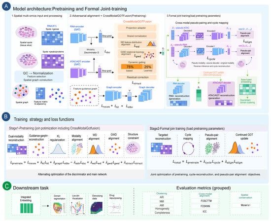
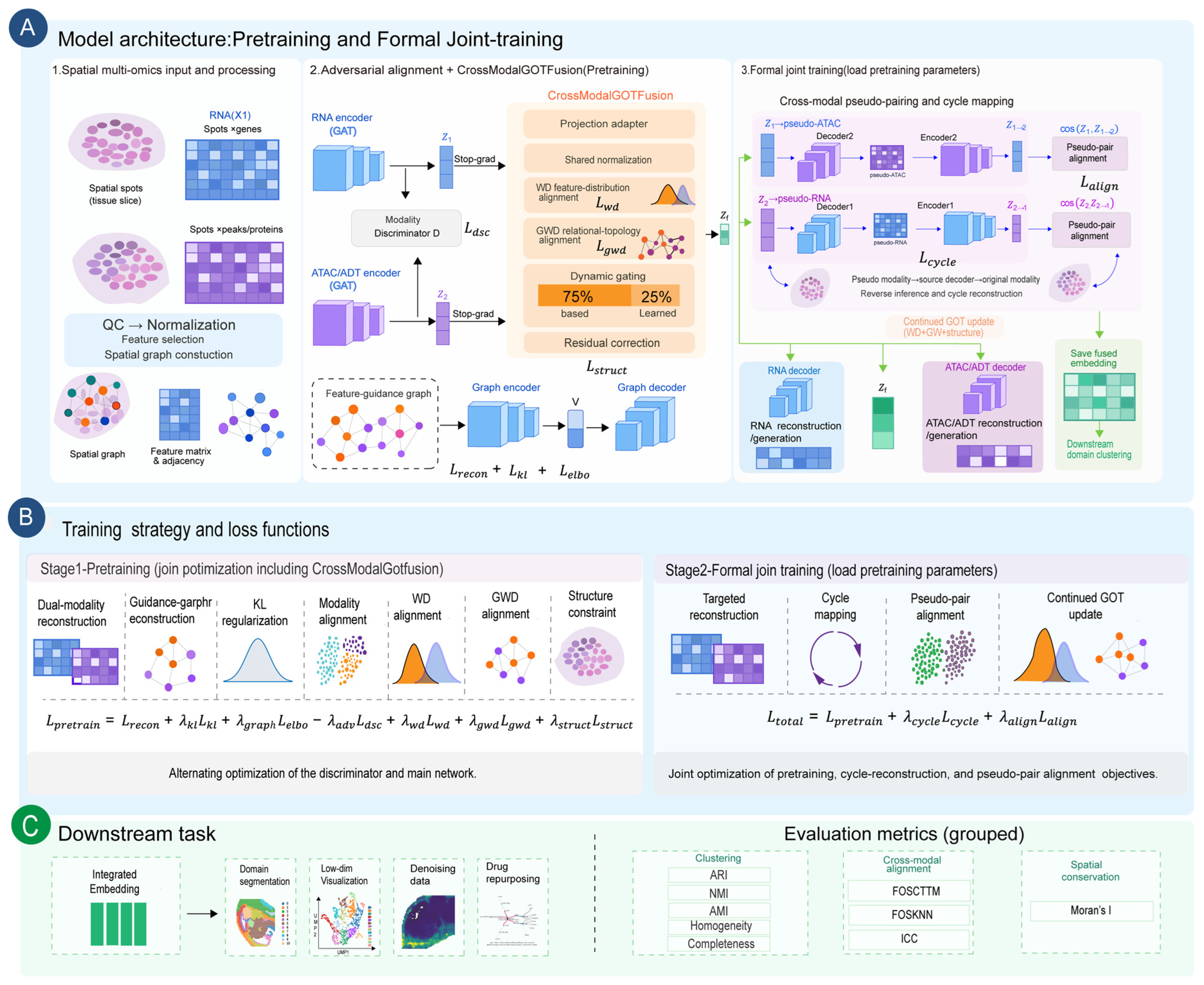
Figure 1 presents the overall architecture and two-stage training strategy of SWINGOT. Spatial multi-omics data, including RNA and ATAC/ADT, are first processed by quality control, normalization, feature selection, and spatial graph construction. The two modalities are then encoded separately by modality-specific Graph Attention Networks to obtain latent representations Z₁ and Z₂. A feature-guidance graph is encoded in parallel to capture relationships among cross-omic features. During pretraining, an adversarial discriminator is used to reduce the global distributional difference between the two modality-specific representations.

Figure 1. Overview of SWINGOT. (A) Model architecture and two-stage training workflow, including spatial multi-omics preprocessing, modality-specific encoding, adversarial alignment, GOT-based fusion, and formal joint training. (B) Training objectives used during pretraining and formal joint training. (C) Downstream analyses and evaluation metrics.

The CrossModalGOTFusion module further integrates the two latent representations. After projection and shared normalization, Wasserstein distance is used to reduce cross-modal distribution differences, while a Gromov–Wasserstein-based loss considers the relational structure within the two latent spaces. The adapted representations are first combined using dynamically learned gating weights, followed by a bounded residual correction. The resulting learned representation is then combined with a stable base representation using a fixed 75%/25% weighting. A structure-preservation loss is used to constrain changes in pairwise relationships among spatial spots. In addition, a stop-gradient operation prevents GOT-related losses from directly updating the backbone encoders.

SWINGOT is trained in two stages. During pretraining, the optimization objectives include dual-modality reconstruction, guidance-graph reconstruction, KL regularization, adversarial modality alignment, Wasserstein alignment, Gromov–Wasserstein-based relational alignment, and structure preservation. In the formal joint-training stage, the pretrained parameters are retained, and cross-modal pseudo-pairing and cycle mapping are activated. Each modality is decoded into the other modality and re-encoded to obtain cross-modal latent representations, which are constrained by cosine-based pseudo-pair alignment. GOT-based alignment and fusion continue to be updated during this stage.

The final fused representation is used for spatial-domain identification, low-dimensional visualization, and downstream molecular analysis. Gene-expression reconstruction uses the modality-specific encoder–decoder pathway. Evaluation includes clustering agreement metrics, Moran’s I for spatial autocorrelation, ICC for within-group consistency, and FOSCTTM and FOSKNN for spot-level cross-modal matching.

2.2.1. Problem Formulation and Overall Architecture

Given a spatial multi-omics dataset containing two modalities (e.g., spatial transcriptomics and epigenomics) measured on the same tissue section, let $X^{\left(A\right)}\in R^{N\times D_A}$ and $X^{\left(B\right)}\in R^{N\times D_B}$ denote the observation matrices for modality A and B, respectively, where N is the number of spatial spots and D_A,D_B are the feature dimensions. Let G^(A) and G^(B) represent their corresponding spatial neighbor graphs.

Let G_f denote the cross-omics feature-guidance graph connecting genes with peaks or proteins.

SWINGOT learns a fused spot representation using a probabilistic dual-encoder backbone, GOT regularization, and conservative residual gated fusion.

The GOT alignment losses and the gated fusion module operate in parallel on the same adapted modality representations. Therefore, WD and GWD act as optimization constraints rather than sequential transformation layers.

2.2.2. Probabilistic Dual-Encoding and Reconstruction

For each modality k ∈ {A,B}, we utilize a Graph Attention Network (GAT)-based data encoder q_ϕ to project the node features and spatial graph into a Gaussian latent space:

Z^(k)~q_ϕ(Z^(k)| X^(k),G^(k)) = N(μ^(k),σ^(k)2)

(1)

The data encoder therefore captures spot-level representations by jointly considering molecular profiles and spatial context. However, spot representations alone do not explicitly encode the regulatory relationships among heterogeneous molecular features.

Simultaneously, a feature graph encoder learns the embedding of features (genes/peaks) $V\in R^{{(D}_A+D_B)\times d}$. The probabilistic decoder p_θ aims to reconstruct the original data based on the data embedding Z^(k) and feature embedding V, scaled by the spot library size l^(k). Z^(k) represents the latent state of each spatial spot, whereas V represents modality-specific features such as genes, peaks, or proteins. The probabilistic modality decoder jointly uses Z^(k), V, and the library-size factor l^(k) to reconstruct the original observation matrix. To accommodate diverse omics distributions, the decoder supports Zero-Inflated Negative Binomial (ZINB), Poisson, or Normal distributions. The base reconstruction loss is the negative log-likelihood:

$$L_{\mathit{recon}}=-{\sum }_{k\in \{A,B\}}{E}_{Z^{\left(k\right)}~q_{\varphi }}\left[\mathit{log}{p}_{\theta }\right(X^{\left(k\right)}|Z^{\left(k\right)},V,l^{\left(k\right)})]$$

(2)

Although reconstruction encourages each modality-specific latent space to retain information from its original observations, it does not ensure correspondence between the two modalities. An adversarial discriminator is used during pretraining to reduce the global difference between the modality-specific latent distributions. The cycle-consistency translation and cosine-based pseudo-pair alignment strategies are activated during formal joint training.

2.2.3. Two-Level Graph Optimal-Transport (GOT) Alignment

Adversarial alignment reduces the global difference between modalities but does not explicitly constrain whether their internal relational structures are preserved. To address this issue, we introduce a two-level Graph Optimal Transport (GOT) module.

First, we apply an adapter network to obtain adapted latents ${\tilde{z}}^{\left(k\right)}=\mathit{LayerNorm}({\mu }^k+{\mathit{MLP}}_k({\mu }^k))$. We define the cross-modal cost matrix $C_{i,j}=1-\cos ({\tilde{Z}}_i^{\left(A\right)},{\tilde{Z}}_j^{\left(B\right)})$. Using the Sinkhorn-Knopp algorithm, we compute the entropy-regularized optimal transport plan P ∈ R^N×N:

$$P=\mathit{arg}\underset{P\in \prod }{\min }⟨P,C⟩+\mathit{ϵH}\left(P\right)$$

(3)

where H(P) is the entropy regularizer. The node-level Wasserstein Distance (WD) loss is defined as L_wd = ⟨P,C⟩. The Wasserstein term establishes cross-modal correspondence at the level of latent points and marginal distributions. However, a low transport cost does not necessarily imply that the internal neighborhood organization of the two modalities is consistent.

To further align the relational structure of the two latent spaces, we introduce a Gromov–Wasserstein-based loss. Let D^(A) and D^(B) denote the intra-modality cosine-distance matrices. To reduce computational cost, we evaluate the squared Gromov–Wasserstein objective using the Sinkhorn transport plan obtained from the cross-modal cost matrix:

$$L_{\mathit{gwd}}={\sum }_{i,j}{{(D}_{\mathit{ij}}^{\left(A\right)})}^2{r}_i{r}_j+{\sum }_{k,l}{{(D}_{\mathit{kl}}^{\left(B\right)})}^2{c}_k{c}_l-2\mathit{Tr}(D^{\left(A\right)}{\mathit{PD}}^{\left(B\right)}{P}^T)$$

(4)

where r and c are the row and column marginals of P.

WD and GWD are computed as parallel regularization objectives on the adapted modality representations. They do not produce an explicitly transported representation that is subsequently passed to the fusion module. Instead, their gradients update the shared projection adapters, progressively improving the representations used by the fusion branch across training iterations. In parallel, the same adapted representations are passed to the conservative residual gated fusion module to generate a single integrated representation.

2.2.4. Conservative Residual Gated Fusion

Using the same adapted modality representations as the GOT alignment branch, the conservative residual gated fusion module generates a single integrated representation. Direct averaging may ignore modality-specific information, while unconstrained nonlinear fusion may distort the original latent structure. We therefore introduce a Conservative Residual Gated Fusion module to obtain an integrated representation while limiting excessive changes to the modality-specific embeddings.

The two adapted modality representations are first combined using dynamically learned gating weights:

$$Z_g={\alpha }_1\widetilde{Z_1}+{\alpha }_2\widetilde{Z_2},{\alpha }_1+{\alpha }_2=1$$

(5)

where α₁ and α₂ determine the relative contribution of the two modalities. A bounded residual correction is then added to obtain the learned fusion representation Z_learn.

To reduce excessive modification of the original latent structure, the final fused representation combines a stable base representation Z_base with the learned representation. The base representation is constructed by L2-normalizing each backbone modality-specific embedding, adding the two normalized embeddings at corresponding spots, and L2-normalizing the result again. Norm denotes row-wise L2 normalization.

Z_f = Norm((1 − β)Z_base + βZ_learn)

(6)

where β is fixed at 0.25 in our experiments. The fixed 75%/25% ratio controls the contributions of the base and learned representations rather than the relative contributions of the two modalities within the dynamic gate.

To further preserve the relationships among spatial spots, we introduce a structure-preservation loss. The average cosine-distance matrix of the two modality-specific representations is used as the reference structure, and a Smooth L1 loss is applied between this reference and the distance matrix of the fused representation:

$$L_{\mathit{structure}}=\mathit{SmoothL}1(D_f,{\displaystyle \frac{D_1+D_2}{2}})$$

(7)

In addition, the modality-specific latent representations are detached before entering the GOT and fusion branch. Therefore, the GOT-related and structure-preservation losses update the fusion module without directly modifying the backbone encoders.

The two modalities are measured at corresponding spatial spots, and this correspondence is used for spot-wise fusion. The optimal transport module does not constrain known spot pairs to hard transport assignments. Instead, it estimates a soft transport plan to regularize cross-modal distributional and relational differences. The current evaluation therefore concerns paired spatial multi-omics data and does not establish performance on unpaired datasets.

2.2.5. Joint Optimization Objective

SWINGOT is trained in two stages. During the first stage, cycle mapping and pseudo-pair alignment are not used. The modality-specific encoders are trained using reconstruction, KL regularization, feature-graph reconstruction, and adversarial alignment, while the GOT and fusion branch are optimized using the Wasserstein, Gromov–Wasserstein, and structure-preservation losses. Because gradient detachment is applied before the GOT branch, these topology-related losses do not directly update the backbone encoders. The pretraining objective is written as follows:

L_pretrain = L_recon + λ_klL_kl + λ_graphL_elbo − λ_advL_dsc + λ_wdL_wd + λ_gwdL_gwd + λ_structL_struct

(8)

In the second stage, the pretrained parameters are retained, and the cycle-consistency translation and cosine-based pseudo-pair alignment inherited are activated.

L_total = L_pretrain + λ_cycleL_cycle + λ_alignL_align

(9)

The λ terms control the relative contribution of the corresponding active loss functions.

Reference labels were not used in the training losses. The fusion coefficient β = 0.25 was selected empirically based on ARI on the labeled E13 dataset. E13 was also included in the final benchmarking, so its reported performance was not evaluated on data independent of fusion-parameter selection. The selected coefficient was then kept fixed across all benchmarking datasets without dataset-specific adjustment. The sensitivity results are reported in Appendix A, Table A4.

3. Results

3.1. Comparison of Model Performance

We evaluated model performance using clustering, spatial coherence, and cross-modal matching metrics. The adjusted Rand index (ARI), normalized mutual information (NMI), and adjusted mutual information (AMI) measure agreement between predicted clusters and reference labels. Homogeneity measures whether each predicted cluster contains spots from a single reference class, while completeness measures whether spots from the same reference class are grouped together. Moran’s I measures spatial autocorrelation, and the intraclass correlation coefficient (ICC) measures within-group consistency. FOSCTTM is the fraction of cross-modal candidates closer than the true match, whereas FOSKNN is the fraction of spots whose true matches fall within their k-nearest neighbors. Higher values indicate better performance for all metrics except FOSCTTM, for which lower values are better. Meanwhile, we bold the best values in all tables.

On the three mouse embryo RNA–ATAC datasets, SWINGOT achieved the highest mean ARI among the compared methods, with values of 0.204, 0.526, and 0.388 on E13, E15, and E18, respectively (Table 2, Table 3 and Table 4). It also achieved the highest mean NMI, AMI, Homogeneity, and Completeness on all three datasets. The mean Moran’s I was highest on E13 and E15, but not on E18, indicating that the improvement in clustering agreement did not extend to every measure of spatial coherence.

Table 2. Model performance on the E13 dataset.

Model	ARI	Moran’s I	ICC	FOSC- TTM	FOS- KNN	NMI	AMI	Homogeneity	Completeness
SWINGOT	0.204 ± 0.004	0.775 ± 0.006	0.004 ± 0.033	0.412 ± 0.018	0.007 ± 0.004	0.418 ± 0.006	0.409 ± 0.005	0.516 ± 0.007	0.352 ± 0.004
SWITCH	0.156 ± 0.010	0.744 ± 0.020	0.140 ± 0.117	0.371 ± 0.036	0.013 ± 0.004	0.351 ± 0.005	0.340 ± 0.005	0.430 ± 0.007	0.296 ± 0.004
SpatialGlue	0.125 ± 0.014	0.669 ± 0.009	0.300 ± 0.043	0.184 ± 0.023	0.079 ± 0.024	0.306 ± 0.014	0.294 ± 0.014	0.372 ± 0.015	0.259 ± 0.013
GLUE	0.150 ± 0.005	0.396 ± 0.033	0.087 ± 0.012	0.269 ± 0.036	0.063 ± 0.007	0.318 ± 0.011	0.307 ± 0.011	0.395 ± 0.014	0.266 ± 0.009
scConfluence	0.165 ± 0.050	0.210 ± 0.046	0.152 ± 0.041	0.334 ± 0.024	0.012 ± 0.001	0.237 ± 0.082	0.224 ± 0.083	0.274 ± 0.089	0.208 ± 0.076
Monae	0.148 ± 0.008	0.334 ± 0.018	0.037 ± 0.028	0.313 ± 0.012	0.020 ± 0.003	0.318 ± 0.007	0.307 ± 0.007	0.396 ± 0.008	0.265 ± 0.006
SCALEX	0.176 ± 0.006	0.354 ± 0.014	0.394 ± 0.004	0.206 ± 0.004	0.060 ± 0.009	0.376 ± 0.006	0.366 ± 0.007	0.467 ± 0.008	0.315 ± 0.006
SIMBA	0.098 ± 0.010	0.288 ± 0.011	−0.219 ± 0.032	0.416 ± 0.008	0.028 ± 0.004	0.234 ± 0.015	0.222 ± 0.016	0.281 ± 0.016	0.201 ± 0.014
LIGER	0.093 ± 0.042	0.101 ± 0.016	−0.124 ± 0.119	0.493 ± 0.006	0.005 ± 0.001	0.141 ± 0.027	0.126 ± 0.027	0.158 ± 0.027	0.127 ± 0.026
MaxFuse	0.049 ± 0.012	0.089 ± 0.012	0.052 ± 0.016	0.427 ± 0.014	0.010 ± 0.003	0.113 ± 0.024	0.099 ± 0.024	0.141 ± 0.030	0.095 ± 0.020

Table 3. Model performance on the E15 dataset.

Model	ARI	Moran’s I	ICC	FOSC- TTM	FOS- KNN	NMI	AMI	Homogeneity	Completeness
SWINGOT	0.526 ± 0.035	0.745 ± 0.013	0.744 ± 0.075	0.102 ± 0.015	0.111 ± 0.026	0.617 ± 0.026	0.611 ± 0.027	0.643 ± 0.029	0.594 ± 0.025
SWITCH	0.477 ± 0.018	0.731 ± 0.020	0.700 ± 0.188	0.113 ± 0.058	0.137 ± 0.059	0.598 ± 0.015	0.592 ± 0.015	0.635 ± 0.019	0.565 ± 0.012
SpatialGlue	0.446 ± 0.010	0.695 ± 0.033	0.255 ± 0.019	0.199 ± 0.013	0.062 ± 0.011	0.587 ± 0.004	0.581 ± 0.004	0.628 ± 0.006	0.552 ± 0.004
GLUE	0.385 ± 0.039	0.514 ± 0.025	0.153 ± 0.013	0.156 ± 0.023	0.127 ± 0.017	0.533 ± 0.024	0.526 ± 0.024	0.576 ± 0.025	0.496 ± 0.023
scConfluence	0.366 ± 0.078	0.339 ± 0.069	0.514 ± 0.080	0.202 ± 0.026	0.042 ± 0.015	0.490 ± 0.063	0.482 ± 0.064	0.514 ± 0.062	0.467 ± 0.064
Monae	0.316 ± 0.027	0.410 ± 0.014	0.113 ± 0.016	0.189 ± 0.009	0.076 ± 0.004	0.503 ± 0.006	0.496 ± 0.006	0.548 ± 0.006	0.465 ± 0.006
SCALEX	0.322 ± 0.010	0.427 ± 0.010	0.477 ± 0.012	0.130 ± 0.005	0.099 ± 0.005	0.501 ± 0.007	0.493 ± 0.008	0.543 ± 0.008	0.465 ± 0.008
SIMBA	0.209 ± 0.021	0.392 ± 0.016	−0.167 ± 0.010	0.341 ± 0.009	0.055 ± 0.007	0.392 ± 0.011	0.383 ± 0.011	0.413 ± 0.009	0.373 ± 0.012
LIGER	0.245 ± 0.012	0.226 ± 0.019	−0.140 ± 0.040	0.455 ± 0.045	0.010 ± 0.003	0.389 ± 0.011	0.380 ± 0.011	0.387 ± 0.012	0.391 ± 0.015
MaxFuse	0.071 ± 0.004	0.122 ± 0.008	0.042 ± 0.009	0.430 ± 0.010	0.010 ± 0.002	0.176 ± 0.009	0.165 ± 0.009	0.193 ± 0.010	0.162 ± 0.008

Table 4. Model performance on the E18 dataset.

Model	ARI	Moran’s I	ICC	FOSC- TTM	FOS- KNN	NMI	AMI	Homogeneity	Completeness
SWINGOT	0.388 ± 0.025	0.641 ± 0.012	0.811 ± 0.026	0.096 ± 0.003	0.120 ± 0.004	0.570 ± 0.006	0.563 ± 0.006	0.622 ± 0.008	0.527 ± 0.006
SWITCH	0.361 ± 0.019	0.659 ± 0.022	0.699 ± 0.228	0.133 ± 0.081	0.104 ± 0.010	0.551 ± 0.021	0.543 ± 0.022	0.600 ± 0.026	0.509 ± 0.017
SpatialGlue	0.355 ± 0.011	0.627 ± 0.005	0.240 ± 0.070	0.224 ± 0.052	0.038 ± 0.009	0.552 ± 0.001	0.544 ± 0.001	0.598 ± 0.001	0.513 ± 0.002
GLUE	0.270 ± 0.007	0.381 ± 0.031	0.087 ± 0.011	0.240 ± 0.014	0.053 ± 0.006	0.474 ± 0.009	0.465 ± 0.010	0.530 ± 0.010	0.429 ± 0.009
scConfluence	0.223 ± 0.060	0.274 ± 0.048	0.262 ± 0.144	0.306 ± 0.068	0.017 ± 0.010	0.393 ± 0.048	0.382 ± 0.049	0.423 ± 0.055	0.366 ± 0.043
Monae	0.298 ± 0.012	0.348 ± 0.015	0.059 ± 0.019	0.201 ± 0.014	0.048 ± 0.007	0.488 ± 0.003	0.479 ± 0.003	0.543 ± 0.003	0.444 ± 0.003
SCALEX	0.281 ± 0.032	0.356 ± 0.014	0.344 ± 0.032	0.230 ± 0.014	0.055 ± 0.024	0.492 ± 0.011	0.483 ± 0.011	0.547 ± 0.012	0.448 ± 0.010
SIMBA	0.331 ± 0.018	0.366 ± 0.022	−0.329 ± 0.017	0.401 ± 0.009	0.025 ± 0.002	0.465 ± 0.006	0.455 ± 0.006	0.488 ± 0.010	0.444 ± 0.003
LIGER	−0.004 ± 0.013	0.070 ± 0.010	−0.036 ± 0.041	0.501 ± 0.003	0.005 ± 0.001	0.086 ± 0.012	0.070 ± 0.012	0.080 ± 0.013	0.093 ± 0.012
MaxFuse	0.032 ± 0.007	0.053 ± 0.009	0.014 ± 0.009	0.473 ± 0.008	0.005 ± 0.001	0.105 ± 0.023	0.090 ± 0.024	0.118 ± 0.026	0.095 ± 0.021

On the human lymph node RNA–ADT dataset, SWINGOT achieved the highest mean ARI of 0.212 and the highest mean Moran’s I of 0.534 among the compared methods (Table 5). It also obtained the highest mean NMI, AMI, Homogeneity, and Completeness, indicating better agreement with the reference domains under the reported evaluation settings.

Table 5. Model performance on the lymph node dataset.

Model	ARI	Moran’s I	ICC	FOSC- TTM	FOS- KNN	NMI	AMI	Homogeneity	Completeness
SWINGOT	0.212 ± 0.019	0.534 ± 0.010	−0.264 ± 0.023	0.575 ± 0.016	0.002 ± 0.001	0.365 ± 0.010	0.361 ± 0.010	0.417 ± 0.006	0.324 ± 0.011
SWITCH	0.160 ± 0.020	0.444 ± 0.044	0.153 ± 0.575	0.389 ± 0.159	0.005 ± 0.002	0.302 ± 0.017	0.298 ± 0.017	0.341 ± 0.014	0.271 ± 0.018
SpatialGlue	0.205 ± 0.002	0.467 ± 0.019	−0.043 ± 0.045	0.569 ± 0.093	0.002 ± 0.001	0.347 ± 0.014	0.343 ± 0.014	0.404 ± 0.018	0.305 ± 0.012
GLUE	0.170 ± 0.011	0.386 ± 0.018	0.061 ± 0.017	0.374 ± 0.014	0.011 ± 0.005	0.309 ± 0.010	0.305 ± 0.010	0.363 ± 0.013	0.269 ± 0.009
scConfluence	0.122 ± 0.012	0.240 ± 0.024	0.105 ± 0.018	0.334 ± 0.009	0.019 ± 0.005	0.198 ± 0.012	0.192 ± 0.012	0.213 ± 0.013	0.184 ± 0.012
Monae	0.130 ± 0.028	0.316 ± 0.034	0.001 ± 0.044	0.489 ± 0.080	0.004 ± 0.002	0.255 ± 0.035	0.250 ± 0.035	0.299 ± 0.041	0.222 ± 0.031
SCALEX	0.097 ± 0.005	0.211 ± 0.006	0.122 ± 0.004	0.373 ± 0.004	0.009 ± 0.003	0.186 ± 0.005	0.180 ± 0.005	0.218 ± 0.006	0.162 ± 0.004
SIMBA	0.078 ± 0.005	0.154 ± 0.010	−0.180 ± 0.008	0.464 ± 0.005	0.011 ± 0.002	0.161 ± 0.006	0.156 ± 0.006	0.189 ± 0.007	0.141 ± 0.006
LIGER	0.091 ± 0.042	0.196 ± 0.012	0.081 ± 0.013	0.398 ± 0.007	0.011 ± 0.003	0.144 ± 0.015	0.138 ± 0.016	0.167 ± 0.017	0.126 ± 0.014
MaxFuse	0.078 ± 0.008	0.198 ± 0.007	0.103 ± 0.003	0.403 ± 0.002	0.010 ± 0.001	0.153 ± 0.005	0.148 ± 0.005	0.180 ± 0.005	0.133 ± 0.004

Cross-modal matching showed a different pattern from clustering agreement. SWINGOT did not consistently achieve the best FOSCTTM or FOSKNN scores across the four datasets, and its ICC performance also varied (Table 2, Table 3, Table 4 and Table 5). Thus, the improvements in spatial-domain identification were not consistently accompanied by better spot-level cross-modal matching or within-group consistency.

Additional experiments examined performance on a breast cancer dataset, the contributions of individual model components, and sensitivity to the fusion coefficient β. The complete model achieved higher ARI than Mean-Fusion on both E13 and the human lymph node dataset, and β = 0.25 achieved the highest mean ARI among the values tested on E13. Detailed settings and results are provided in Appendix A, Table A1, Table A2, Table A3 and Table A4. Additional statistical comparisons based on three random-seed runs on E15 are provided in Appendix A.5 (Figure A2).

3.2. Spatial Domain Identification in Mouse Embryos

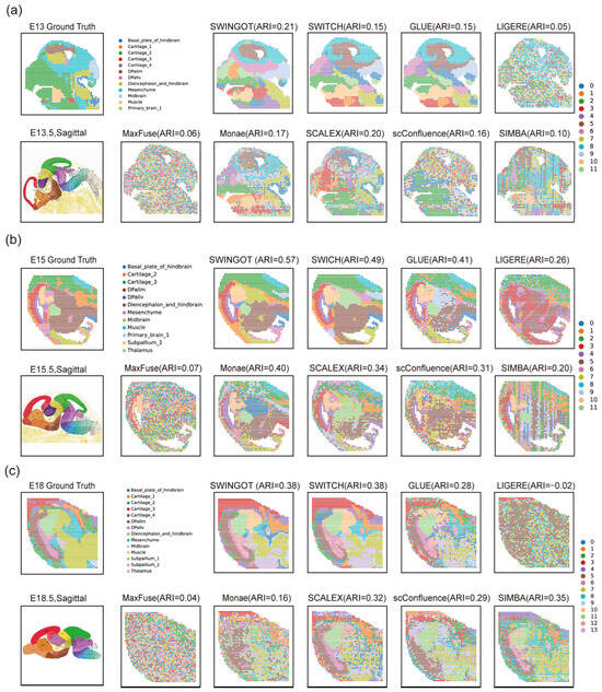
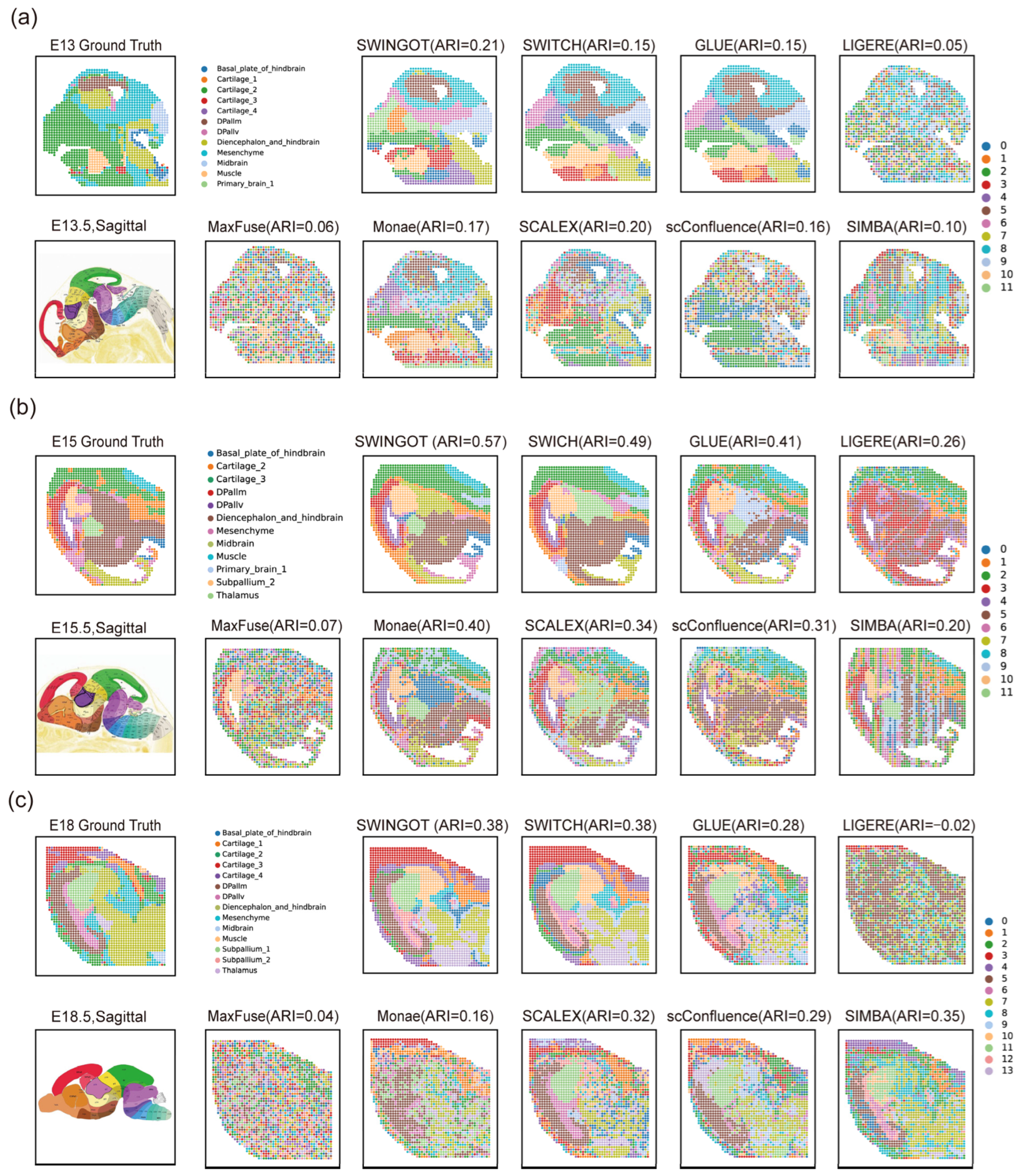
We visualized the identified domains on the original tissue coordinates to examine their spatial organization (Figure 2). Several comparison methods produced fragmented assignments, with neighboring spots frequently assigned to different clusters. SWINGOT recovered more continuous domains in several tissue regions, although some boundaries differed from the reference annotation.

Figure 2. Comparison of spatial-domain identification results on the mouse embryo datasets. (a) E13 mouse embryo RNA–ATAC dataset. (b) E15 mouse embryo RNA–ATAC dataset. (c) E18 mouse embryo RNA–ATAC dataset. Ground-truth annotations and results from different integration methods are shown, with ARI values indicated for each method. The ARI values correspond to the displayed clustering results. Aggregate performance is reported in Table 2, Table 3 and Table 4.

In the displayed E15 result, SWINGOT recovered several continuous regions that broadly followed the reference tissue organization. On E18, the identified domains also showed spatial continuity, although some boundaries differed from the reference annotation (Figure 2).

3.3. Low-Dimensional Visualization of Integrated Representations

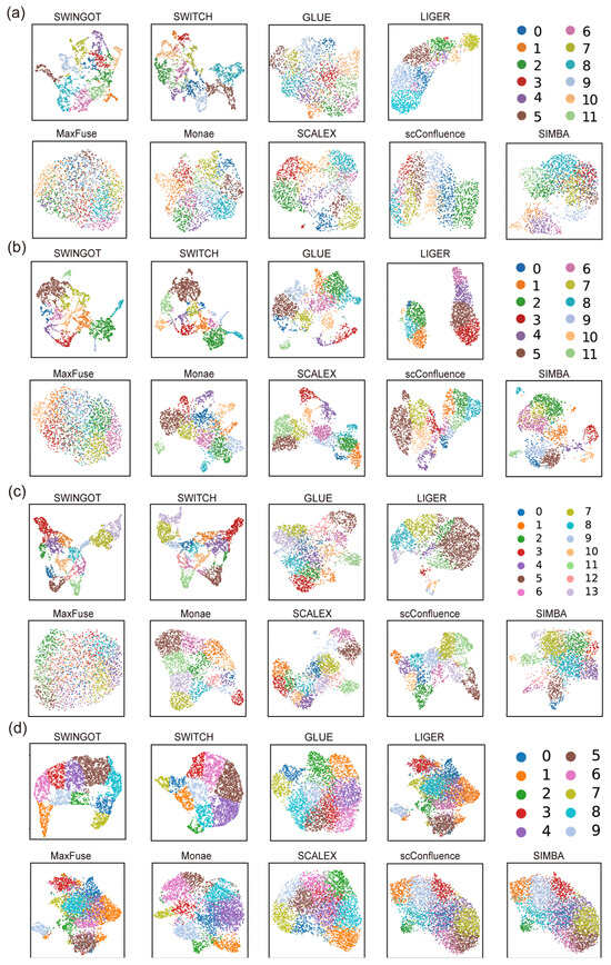
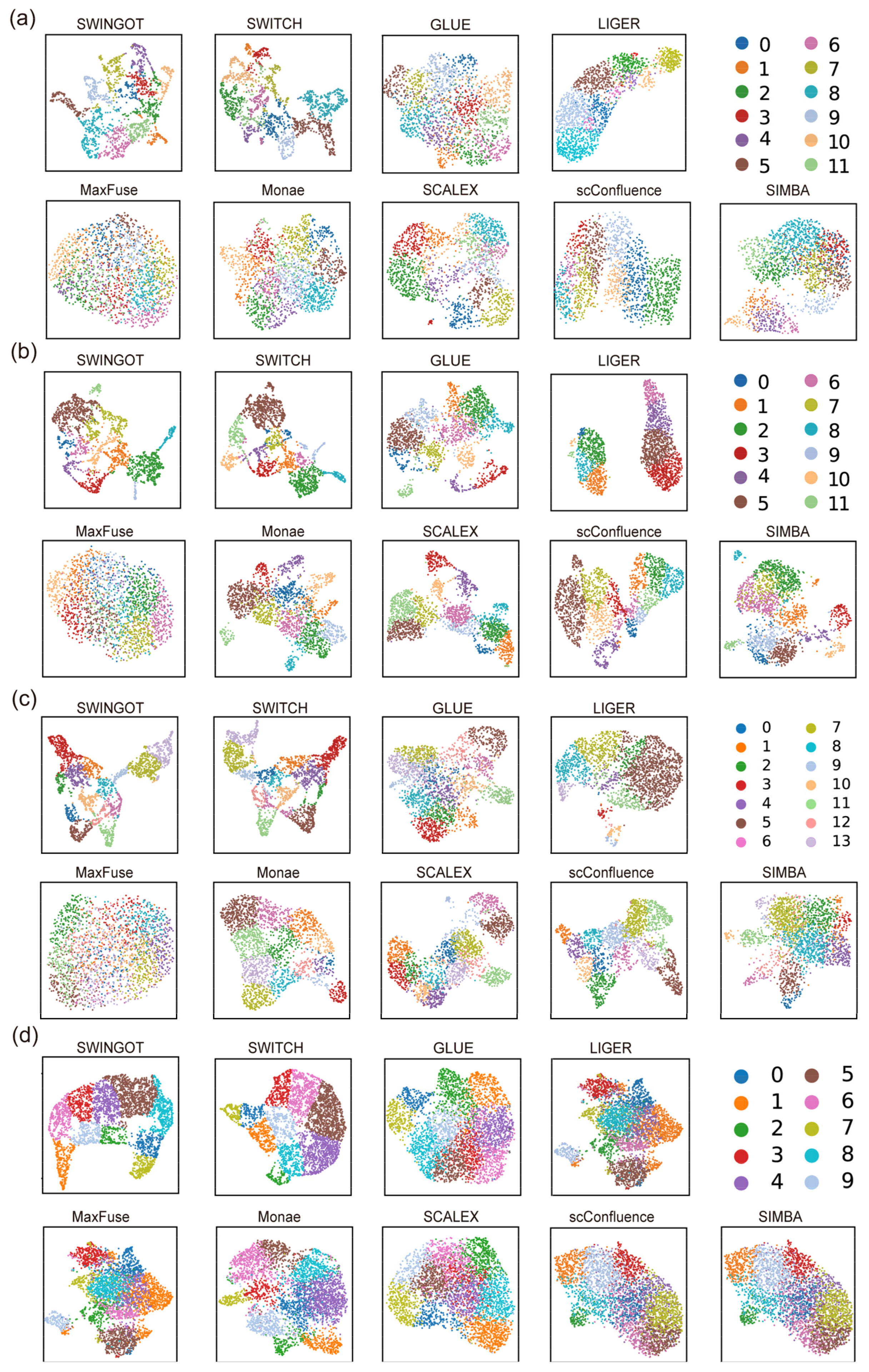
To examine the organization of the integrated representations, we visualized the embeddings generated by different methods using UMAP (Figure 3). Spots were colored according to their reference spatial-domain labels, allowing the organization of known spatial domains in each latent space to be compared across methods.

Figure 3. UMAP visualization of the integrated representations generated by different multi-omics integration methods. UMAP embeddings are shown for (a) the E13 mouse embryo RNA–ATAC dataset; (b) the E15 mouse embryo RNA–ATAC dataset; (c) the E18 mouse embryo RNA–ATAC dataset; and (d) the human lymph node RNA–ADT dataset. Each point represents a spatial spot, and colors indicate the reference spatial-domain labels.

In E15 and E18, several reference domains occupied distinguishable regions in the SWINGOT UMAP plots. More overlap was observed in E13. The human lymph node representation also showed separation among several domains, with partial overlap remaining. These plots describe the two-dimensional organization of the embeddings; the quantitative comparisons are reported in Table 2, Table 3, Table 4 and Table 5.

3.4. Spatial Denoising of Marker-Gene Expression in the E18 Embryo

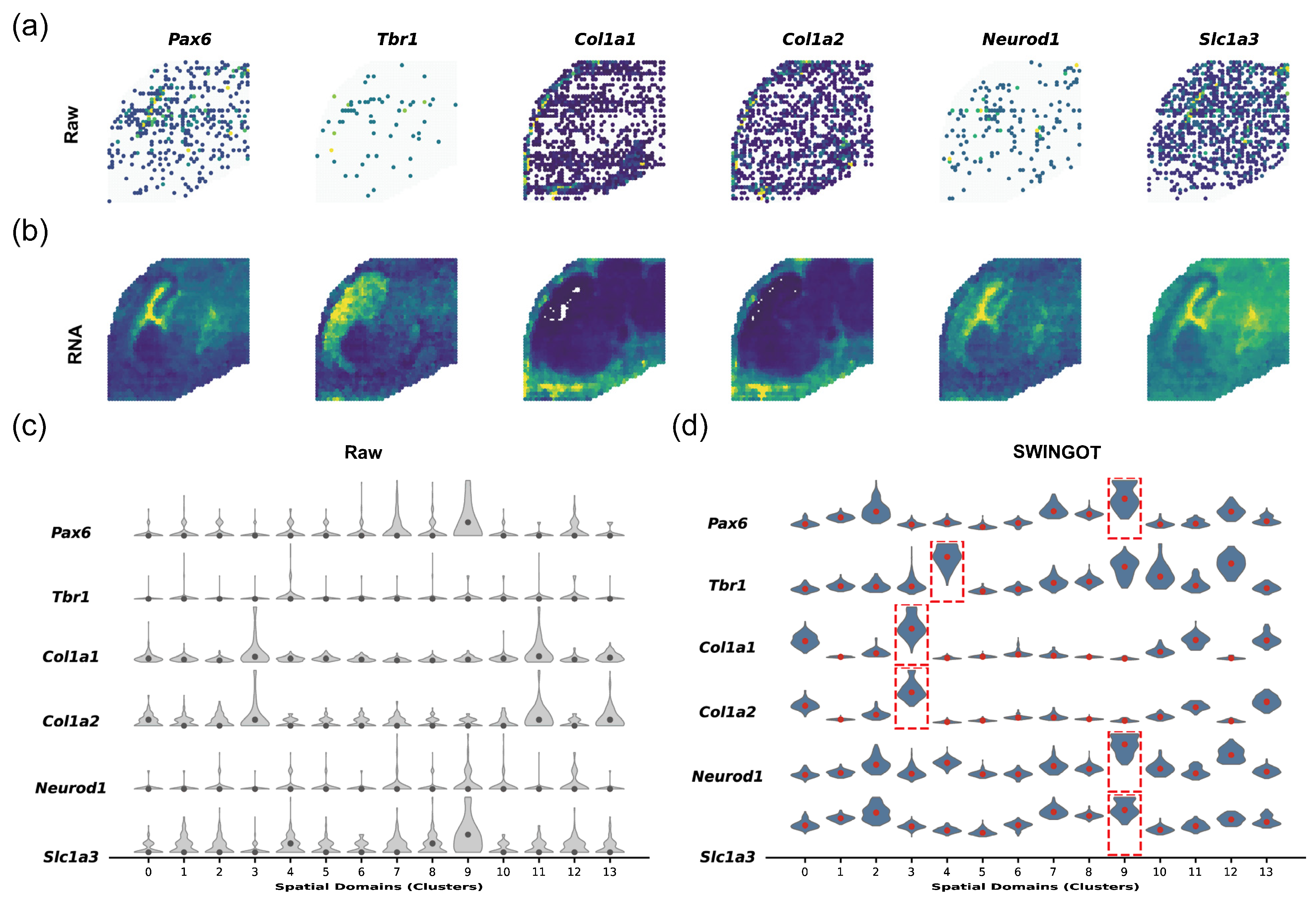
We examined reconstructed RNA expression in the E18 mouse embryo using six genes with reported developmental and tissue-associated expression patterns. Pax6 and Slc1a3 are associated with neural progenitor and radial glial populations. Neurod1 is associated with neuronal differentiation, while Tbr1 is expressed in postmitotic cortical neurons. Col1a1 and Col1a2 encode type I collagen chains and are expressed by fibroblasts, including meningeal fibroblasts. This panel provided examples of neural and connective-tissue-associated expression for comparing the raw and reconstructed spatial patterns.

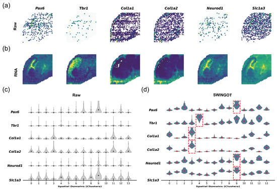
In the raw RNA data, the expression patterns of several genes were relatively sparse and spatially discontinuous (Figure 4a). After reconstruction, the corresponding expression patterns became more spatially continuous and showed clearer regional enrichment (Figure 4b).

Figure 4. Spatial expression patterns and denoising of representative marker genes in the E18 mouse embryo dataset. (a) Raw spatial expression patterns of six representative genes, including Pax6, Tbr1, Col1a1, Col1a2, Neurod1, and Slc1a3. (b) Spatial expression patterns of the corresponding genes after SWINGOT processing. (c) Expression distributions of the six genes across 14 spatial domains in the raw RNA data. (d) Expression distributions after SWINGOT processing. Red dashed boxes indicate spatial domains showing enriched expression of the corresponding genes.

We further compared the expression distributions of these genes across the 14 spatial domains. In the raw data, several marker genes showed relatively dispersed expression across multiple domains (Figure 4c). After processing, their expression became more concentrated in specific spatial domains, with clearer domain-associated enrichment patterns (Figure 4d).

The spatial maps and violin plots provide some evidence that the reconstructed data retain regional expression patterns. Additional evaluation of spatial organization and held-out RNA-count prediction on E18 is provided in Appendix A.6 (Figure A3). The results support improved held-out prediction over the tested simple spatial-smoothing baseline but do not exclude excessive smoothing or loss of local biological variation.

3.5. Spatial Heterogeneity and Downstream Analysis in the Human Lymph Node

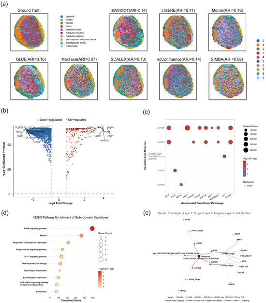
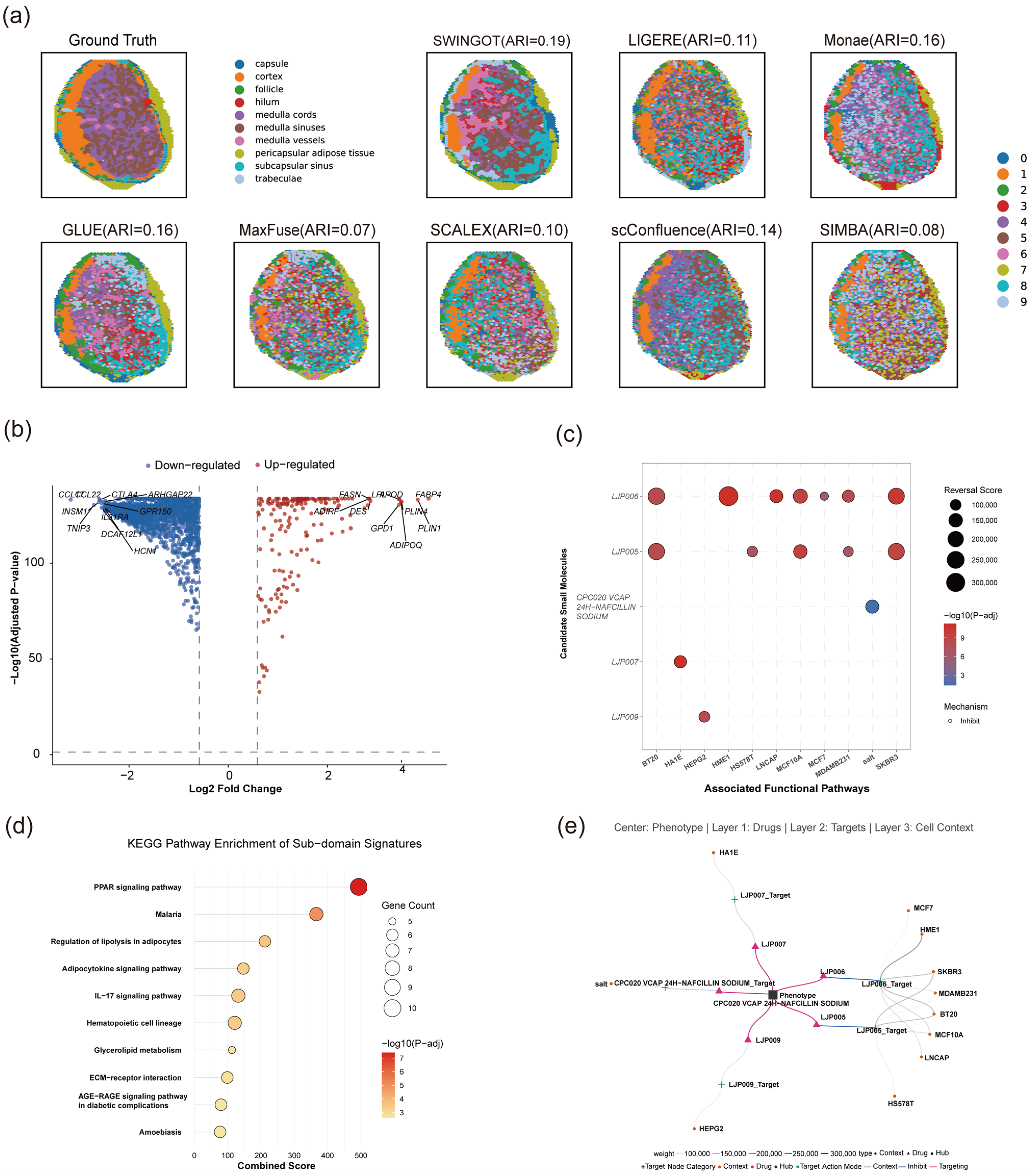
We examined the molecular differences among selected spatial regions in the human lymph node dataset. In the displayed clustering result, SWINGOT recovered several continuous regions and produced fewer scattered assignments than several comparison methods (Figure 5a). The aggregate clustering results are reported in Table 5.

Figure 5. Spatial heterogeneity and downstream molecular analysis of the human lymph node dataset. (a) Spatial-domain identification results obtained by SWINGOT and comparison methods, together with the reference annotation. ARI values are shown for each method; (b) differentially expressed genes between selected spatial regions; (c) candidate compounds identified from LINCS L1000 perturbation signatures; (d) KEGG pathway enrichment analysis of the differential gene signature; (e) network linking candidate compounds with associated targets and cellular contexts.

Differential-expression analysis identified distinct expression patterns between the selected regions (Figure 5b). Lipid metabolism- and adipocyte-associated genes, including FASN, FABP4, and ADIPOQ, showed higher expression in one region, while immune-related genes such as CCL21 and CTLA4 differed between regions. KEGG analysis identified enrichment of PPAR signaling, regulation of lipolysis in adipocytes, and adipocytokine signaling (Figure 5d).

The differential gene signature was also used to query LINCS L1000 for perturbation signatures with opposite transcriptional changes. Candidate compounds and their cellular contexts are summarized in Figure 5c,e. These results identify computational candidates for further study. Regional expression differences in this lymph node sample do not by themselves establish a disease signature or a therapeutic effect.

4. Discussion

SWINGOT achieved the highest mean ARI among the compared methods on the three mouse embryo datasets and the human lymph node dataset. Its performance was less consistent across spatial coherence, cross-modal matching, and within-group consistency metrics. These results indicate that agreement with reference spatial domains, spatial coherence, and spot-level cross-modal matching capture different aspects of integration and should be assessed separately.

The ablation experiments (Table A2 and Table A3) assessed the added alignment and fusion branch for spatial-domain identification. Replacing the proposed fusion strategy with mean fusion reduced ARI on both E13 and the human lymph node dataset. Removing the WD- or GW-based loss also reduced ARI, although the size of the decrease depended on the dataset. On the human lymph node dataset, removing both alignment losses produced a higher ARI than removing either loss alone, showing that their effects were not additive. These experiments evaluate the proposed fusion strategy as a whole and do not separately establish the contribution of each operation within it.

The sensitivity analysis (Table A4) showed that the fusion coefficient affected spatial-domain identification. On E13, β = 0.25 achieved the highest mean ARI among the tested values. Increasing β above 0.25 did not further improve ARI, although some settings achieved better Moran’s I or cross-modal matching scores. The selected value therefore reflects the emphasis on spatial-domain identification. Reference labels were not used in the training losses, but ARI on labeled datasets was used to select β during development. Further assessment on independent datasets is needed to determine how well this setting transfers to other data.

The additional breast cancer evaluation (Table A1) extended the analysis to a disease-related RNA–ADT dataset. SWINGOT achieved the highest mean Moran’s I and the lowest CHAOS score, but it did not achieve the best PAS, ASW_spatial, ICC, or cross-modal matching results. These findings support its ability to recover spatially coherent domains in an additional setting. Because reference domain annotations were unavailable for this evaluation, the spatial metrics alone do not establish that the identified regions correspond to the correct biological boundaries.

The E18 expression plots and count-splitting analysis support regional expression patterns and improved held-out prediction over the tested spatial-smoothing baseline, although excessive smoothing cannot be ruled out. Denoising uses the modality-specific encoder–decoder pathway and should not be treated as direct evidence of improvement from the GOT fusion module. In the human lymph node dataset, differential-expression and pathway analyses identified lipid-related and immune-related differences among selected regions. The LINCS results remain computational candidates and do not establish therapeutic efficacy.

Several limitations remain. The evaluation covers a limited number of tissues, developmental stages, and spatial multi-omics technologies. The contribution of each model component and the choice of β may depend on the dataset and evaluation objective. Denoising accuracy and the stability of downstream pathway and compound findings have not been independently established. Further studies using additional datasets and experimental evidence are needed to assess these aspects.

5. Conclusions

In this study, we introduced SWINGOT, a strategy for integrating paired spatial multi-omics data using Wasserstein-based distribution alignment, GW-based relational regularization, and conservative residual gated fusion. The method combines modality-specific information while constraining changes in the relationships among spatial spots.

SWINGOT achieved the highest mean ARI among the compared methods on three mouse embryo RNA–ATAC datasets and a human lymph node RNA–ADT dataset. The ablation experiments supported the contribution of the additional components to spatial-domain identification, while the sensitivity analysis showed that performance depended on the fusion coefficient. The breast cancer evaluation provided further evidence of spatial coherence in an additional RNA–ADT dataset. Cross-modal matching did not improve consistently across datasets.

The fused representations supported spatial-domain identification and downstream molecular analyses, while gene-expression reconstruction used the modality-specific encoder–decoder pathway. The reconstruction, pathway, and compound-related findings require further validation. Future evaluation across additional tissues and technologies will help determine the range of settings in which the method is useful.

Appendix A.1

We evaluated SWINGOT on an additional breast cancer dataset containing paired spatial RNA and protein measurements. Reference spatial-domain annotations were unavailable for this evaluation, and the number of clusters was set to 10. Annotation-based clustering metrics, including ARI, were therefore not reported.

Spatial organization was assessed using Moran’s I, CHAOS, the percentage of abnormal spots (PAS), and spatial average silhouette width (ASW_spatial). CHAOS summarizes local spatial discontinuity within identified domains, PAS measures disagreement between a spot’s domain label and those of its spatial neighbors, and ASW_spatial summarizes domain compactness and separation. Lower CHAOS and PAS values and higher Moran’s I and ASW_spatial values indicate better performance. ICC, FOSCTTM, and FOSKNN were also reported to assess within-group consistency and cross-modal matching.

Table A1. Model performance on the breast cancer dataset.

Model	Moran’s I	CHAOS	ASW spatial	ICC	FOSC-TTM	FOS-KNN	PAS
SWINGOT	0.576 ± 0.021	0.058 ± 0.001	0.450 ± 0.002	−0.048 ± 0.212	0.646 ± 0.078	0.001 ± 0.001	0.314 ± 0.028
SWITCH	0.486 ± 0.022	0.060 ± 0.001	0.453 ± 0.006	0.228 ± 0.093	0.281 ± 0.067	0.010 ± 0.002	0.423 ± 0.026
SpatialGlue	0.562 ± 0.024	0.059 ± 0.001	0.437 ± 0.006	−0.033 ± 0.053	0.558 ± 0.125	0.001 ± 0.001	0.288 ± 0.017
GLUE	0.480 ± 0.010	0.063 ± 0.001	0.430 ± 0.013	−0.003 ± 0.038	0.509 ± 0.108	0.002 ± 0.002	0.436 ± 0.012
scConfluence	0.463 ± 0.021	0.060 ± 0.001	0.385 ± 0.042	0.722 ± 0.012	0.040 ± 0.003	0.192 ± 0.037	0.431 ± 0.007
Monae	0.494 ± 0.038	0.061 ± 0.000	0.442 ± 0.007	0.185 ± 0.069	0.169 ± 0.092	0.040 ± 0.022	0.411 ± 0.061
SCALEX	0.360 ± 0.007	0.064 ± 0.000	0.440 ± 0.003	0.280 ± 0.013	0.186 ± 0.008	0.023 ± 0.001	0.599 ± 0.022
SIMBA	0.288 ± 0.005	0.070 ± 0.000	0.431 ± 0.001	0.021 ± 0.007	0.298 ± 0.002	0.029 ± 0.001	0.675 ± 0.006
LIGER	0.315 ± 0.014	0.068 ± 0.001	0.434 ± 0.002	0.250 ± 0.005	0.245 ± 0.014	0.019 ± 0.004	0.634 ± 0.023
MaxFuse	0.371 ± 0.016	0.068 ± 0.001	0.437 ± 0.002	0.248 ± 0.011	0.264 ± 0.009	0.022 ± 0.001	0.577 ± 0.027

Table A1. Model performance on the breast cancer dataset.

Model	Moran’s I	CHAOS	ASW spatial	ICC	FOSC-TTM	FOS-KNN	PAS
SWINGOT	0.576 ± 0.021	0.058 ± 0.001	0.450 ± 0.002	−0.048 ± 0.212	0.646 ± 0.078	0.001 ± 0.001	0.314 ± 0.028
SWITCH	0.486 ± 0.022	0.060 ± 0.001	0.453 ± 0.006	0.228 ± 0.093	0.281 ± 0.067	0.010 ± 0.002	0.423 ± 0.026
SpatialGlue	0.562 ± 0.024	0.059 ± 0.001	0.437 ± 0.006	−0.033 ± 0.053	0.558 ± 0.125	0.001 ± 0.001	0.288 ± 0.017
GLUE	0.480 ± 0.010	0.063 ± 0.001	0.430 ± 0.013	−0.003 ± 0.038	0.509 ± 0.108	0.002 ± 0.002	0.436 ± 0.012
scConfluence	0.463 ± 0.021	0.060 ± 0.001	0.385 ± 0.042	0.722 ± 0.012	0.040 ± 0.003	0.192 ± 0.037	0.431 ± 0.007
Monae	0.494 ± 0.038	0.061 ± 0.000	0.442 ± 0.007	0.185 ± 0.069	0.169 ± 0.092	0.040 ± 0.022	0.411 ± 0.061
SCALEX	0.360 ± 0.007	0.064 ± 0.000	0.440 ± 0.003	0.280 ± 0.013	0.186 ± 0.008	0.023 ± 0.001	0.599 ± 0.022
SIMBA	0.288 ± 0.005	0.070 ± 0.000	0.431 ± 0.001	0.021 ± 0.007	0.298 ± 0.002	0.029 ± 0.001	0.675 ± 0.006
LIGER	0.315 ± 0.014	0.068 ± 0.001	0.434 ± 0.002	0.250 ± 0.005	0.245 ± 0.014	0.019 ± 0.004	0.634 ± 0.023
MaxFuse	0.371 ± 0.016	0.068 ± 0.001	0.437 ± 0.002	0.248 ± 0.011	0.264 ± 0.009	0.022 ± 0.001	0.577 ± 0.027

SWINGOT achieved the highest mean Moran’s I of 0.576 ± 0.021 and the lowest CHAOS score of 0.058 ± 0.001 among the compared methods (Table A1). Its PAS was lower than that of SWITCH (0.314 ± 0.028 versus 0.423 ± 0.026), although SpatialGlue achieved a lower value of 0.288 ± 0.017. SWINGOT obtained an ASW_spatial of 0.450 ± 0.002, close to the value of 0.453 ± 0.006 obtained by SWITCH.

The results were less favorable for within-group consistency and cross-modal matching. SWINGOT obtained an ICC of −0.048 ± 0.212, a FOSCTTM of 0.646 ± 0.078, and a FOSKNN of 0.001 ± 0.001. These results show that its performance in spatial coherence did not extend to all aspects of integration. Because reference domain annotations were unavailable, this evaluation supports conclusions about spatial organization but does not establish the biological accuracy of the identified boundaries.

Appendix A.2

We performed component ablation analyses on E13 and the human lymph node dataset. No WD removes the Wasserstein loss, No GW removes the GW-based relational loss, and No OT removes both transport-based losses. Mean-Fusion replaces the proposed fusion strategy with simple mean fusion. No Struct removes the structure-preservation loss and was evaluated on the human lymph node dataset. The results are reported in Table A2 and Table A3.

Table A2. Ablation results on the E13 dataset.

Model	ARI	Moran’s I	ICC	FOSC- TTM	FOS- KNN	NMI	AMI	Homogeneity	Completeness
Full	0.204 ± 0.004	0.775 ± 0.006	0.004 ± 0.033	0.412 ± 0.018	0.007 ± 0.004	0.418 ± 0.006	0.409 ± 0.005	0.516 ± 0.007	0.352 ± 0.004
No WD	0.183 ± 0.010	0.765 ± 0.004	0.093 ± 0.156	0.368 ± 0.067	0.019 ± 0.017	0.399 ± 0.008	0.390 ± 0.008	0.494 ± 0.011	0.335 ± 0.006
No GW	0.191 ± 0.012	0.762 ± 0.018	0.084 ± 0.133	0.363 ± 0.057	0.022 ± 0.014	0.403 ± 0.012	0.394 ± 0.012	0.498 ± 0.015	0.339 ± 0.010
No OT	0.183 ± 0.014	0.768 ± 0.016	0.040 ± 0.141	0.366 ± 0.057	0.023 ± 0.016	0.403 ± 0.015	0.393 ± 0.015	0.499 ± 0.020	0.338 ± 0.013
Mean-Fusion	0.133 ± 0.005	0.722 ± 0.023	0.109 ± 0.149	0.365 ± 0.075	0.021 ± 0.018	0.334 ± 0.004	0.324 ± 0.005	0.412 ± 0.009	0.282 ± 0.002

Table A2. Ablation results on the E13 dataset.

Model	ARI	Moran’s I	ICC	FOSC- TTM	FOS- KNN	NMI	AMI	Homogeneity	Completeness
Full	0.204 ± 0.004	0.775 ± 0.006	0.004 ± 0.033	0.412 ± 0.018	0.007 ± 0.004	0.418 ± 0.006	0.409 ± 0.005	0.516 ± 0.007	0.352 ± 0.004
No WD	0.183 ± 0.010	0.765 ± 0.004	0.093 ± 0.156	0.368 ± 0.067	0.019 ± 0.017	0.399 ± 0.008	0.390 ± 0.008	0.494 ± 0.011	0.335 ± 0.006
No GW	0.191 ± 0.012	0.762 ± 0.018	0.084 ± 0.133	0.363 ± 0.057	0.022 ± 0.014	0.403 ± 0.012	0.394 ± 0.012	0.498 ± 0.015	0.339 ± 0.010
No OT	0.183 ± 0.014	0.768 ± 0.016	0.040 ± 0.141	0.366 ± 0.057	0.023 ± 0.016	0.403 ± 0.015	0.393 ± 0.015	0.499 ± 0.020	0.338 ± 0.013
Mean-Fusion	0.133 ± 0.005	0.722 ± 0.023	0.109 ± 0.149	0.365 ± 0.075	0.021 ± 0.018	0.334 ± 0.004	0.324 ± 0.005	0.412 ± 0.009	0.282 ± 0.002

Table A3. Ablation results on the lymph node dataset.

Model	ARI	Moran’s I	ICC	FOSC- TTM	FOS- KNN	NMI	AMI	Homogeneity	Completeness
Full	0.212 ± 0.019	0.534 ± 0.010	−0.264 ± 0.023	0.575 ± 0.016	0.002 ± 0.001	0.365 ± 0.010	0.361 ± 0.010	0.417 ± 0.006	0.324 ± 0.011
No WD	0.162 ± 0.009	0.473 ± 0.052	0.195 ± 0.705	0.439 ± 0.153	0.005 ± 0.003	0.310 ± 0.012	0.306 ± 0.012	0.356 ± 0.021	0.275 ± 0.006
No GW	0.153 ± 0.013	0.433 ± 0.077	0.182 ± 0.711	0.434 ± 0.149	0.006 ± 0.003	0.300 ± 0.024	0.296 ± 0.025	0.342 ± 0.034	0.267 ± 0.019
No OT	0.170 ± 0.009	0.515 ± 0.028	−0.216 ± 0.650	0.487 ± 0.178	0.004 ± 0.003	0.321 ± 0.006	0.317 ± 0.006	0.371 ± 0.003	0.283 ± 0.008
No Struct	0.146 ± 0.008	0.421 ± 0.051	0.208 ± 0.727	0.447 ± 0.135	0.005 ± 0.001	0.278 ± 0.008	0.274 ± 0.008	0.311 ± 0.014	0.252 ± 0.004
Mean-Fusion	0.141 ± 0.003	0.399 ± 0.025	0.174 ± 0.744	0.436 ± 0.150	0.005 ± 0.004	0.268 ± 0.030	0.263 ± 0.030	0.301 ± 0.036	0.241 ± 0.026

Table A3. Ablation results on the lymph node dataset.

Model	ARI	Moran’s I	ICC	FOSC- TTM	FOS- KNN	NMI	AMI	Homogeneity	Completeness
Full	0.212 ± 0.019	0.534 ± 0.010	−0.264 ± 0.023	0.575 ± 0.016	0.002 ± 0.001	0.365 ± 0.010	0.361 ± 0.010	0.417 ± 0.006	0.324 ± 0.011
No WD	0.162 ± 0.009	0.473 ± 0.052	0.195 ± 0.705	0.439 ± 0.153	0.005 ± 0.003	0.310 ± 0.012	0.306 ± 0.012	0.356 ± 0.021	0.275 ± 0.006
No GW	0.153 ± 0.013	0.433 ± 0.077	0.182 ± 0.711	0.434 ± 0.149	0.006 ± 0.003	0.300 ± 0.024	0.296 ± 0.025	0.342 ± 0.034	0.267 ± 0.019
No OT	0.170 ± 0.009	0.515 ± 0.028	−0.216 ± 0.650	0.487 ± 0.178	0.004 ± 0.003	0.321 ± 0.006	0.317 ± 0.006	0.371 ± 0.003	0.283 ± 0.008
No Struct	0.146 ± 0.008	0.421 ± 0.051	0.208 ± 0.727	0.447 ± 0.135	0.005 ± 0.001	0.278 ± 0.008	0.274 ± 0.008	0.311 ± 0.014	0.252 ± 0.004
Mean-Fusion	0.141 ± 0.003	0.399 ± 0.025	0.174 ± 0.744	0.436 ± 0.150	0.005 ± 0.004	0.268 ± 0.030	0.263 ± 0.030	0.301 ± 0.036	0.241 ± 0.026

On E13, the complete model achieved the highest mean ARI of 0.204 ± 0.004 (Table A2). Removing the WD- or GW-based loss reduced ARI to 0.183 ± 0.010 and 0.191 ± 0.012, respectively. Removing both losses resulted in an ARI of 0.183 ± 0.014. Mean-Fusion produced a larger decrease to 0.133 ± 0.005. The complete model also achieved the highest mean NMI, AMI, Homogeneity, Completeness, and Moran’s I. These comparisons support the contribution of the proposed fusion strategy to spatial-domain identification, with smaller ARI improvements associated with the individual transport-based objectives.

On the human lymph node dataset, the complete model achieved the highest mean ARI of 0.212 ± 0.019 (Table A3). ARI decreased to 0.162 without WD, 0.153 without GW-based regularization, and 0.170 without both losses. Removing the structure-preservation loss reduced ARI to 0.146, while Mean-Fusion obtained 0.141. The complete model also achieved the highest mean Moran’s I, NMI, AMI, Homogeneity, and Completeness.

The effects of the alignment losses were not additive: No OT achieved a higher ARI than either No WD or No GW. Thus, the results support evaluating these objectives as interacting parts of the model and do not show that each term contributes a fixed, independent improvement.

The cross-modal matching metrics did not follow the same ordering as the clustering metrics. On E13, No GW obtained a lower FOSCTTM than the complete model (0.363 versus 0.412), while No OT obtained a higher FOSKNN (0.023 versus 0.007). On the human lymph node dataset, No GW also obtained a lower FOSCTTM and a higher FOSKNN than the complete model. These reported differences show that the setting with the best spatial-domain agreement did not also provide the best spot-level matching. They do not by themselves establish a causal trade-off between the loss functions and matching accuracy.

Appendix A.3

We examined sensitivity to the fusion coefficient β on E13 using values of 0, 0.25, 0.50, 0.75, and 1.00. In Equation (6), β controls the contribution of the learned fusion representation, while 1 − β controls the contribution of the base representation. At β = 0, the final representation contains only the base representation; at β = 1, it contains only the learned representation. The results are summarized in Table A4.

Table A4. Sensitivity to the fusion coefficient β on the E13 dataset.

β	ARI	Moran’s I	ICC	FOSC- TTM	FOS- KNN	NMI	AMI	Homog- eneity	Complet-eness
0	0.133 ± 0.005	0.722 ± 0.023	0.109 ± 0.149	0.365 ± 0.075	0.021 ± 0.018	0.334 ± 0.004	0.324 ± 0.005	0.412 ± 0.009	0.282 ± 0.002
0.25 (paper)	0.204 ± 0.004	0.775 ± 0.006	0.004 ± 0.033	0.412 ± 0.018	0.007 ± 0.004	0.418 ± 0.006	0.409 ± 0.005	0.516 ± 0.007	0.352 ± 0.004
0.5	0.178 ± 0.012	0.767 ± 0.018	0.070 ± 0.159	0.365 ± 0.074	0.020 ± 0.016	0.392 ± 0.018	0.382 ± 0.018	0.483 ± 0.022	0.330 ± 0.015
0.75	0.174 ± 0.003	0.780 ± 0.003	0.065 ± 0.168	0.362 ± 0.061	0.023 ± 0.015	0.410 ± 0.007	0.400 ± 0.007	0.508 ± 0.010	0.343 ± 0.006
1.0	0.172 ± 0.002	0.778 ± 0.013	0.046 ± 0.133	0.369 ± 0.072	0.018 ± 0.017	0.401 ± 0.014	0.391 ± 0.014	0.497 ± 0.018	0.336 ± 0.011

Table A4. Sensitivity to the fusion coefficient β on the E13 dataset.

β	ARI	Moran’s I	ICC	FOSC- TTM	FOS- KNN	NMI	AMI	Homog- eneity	Complet-eness
0	0.133 ± 0.005	0.722 ± 0.023	0.109 ± 0.149	0.365 ± 0.075	0.021 ± 0.018	0.334 ± 0.004	0.324 ± 0.005	0.412 ± 0.009	0.282 ± 0.002
0.25 (paper)	0.204 ± 0.004	0.775 ± 0.006	0.004 ± 0.033	0.412 ± 0.018	0.007 ± 0.004	0.418 ± 0.006	0.409 ± 0.005	0.516 ± 0.007	0.352 ± 0.004
0.5	0.178 ± 0.012	0.767 ± 0.018	0.070 ± 0.159	0.365 ± 0.074	0.020 ± 0.016	0.392 ± 0.018	0.382 ± 0.018	0.483 ± 0.022	0.330 ± 0.015
0.75	0.174 ± 0.003	0.780 ± 0.003	0.065 ± 0.168	0.362 ± 0.061	0.023 ± 0.015	0.410 ± 0.007	0.400 ± 0.007	0.508 ± 0.010	0.343 ± 0.006
1.0	0.172 ± 0.002	0.778 ± 0.013	0.046 ± 0.133	0.369 ± 0.072	0.018 ± 0.017	0.401 ± 0.014	0.391 ± 0.014	0.497 ± 0.018	0.336 ± 0.011

The mean ARI values were 0.133, 0.204, 0.178, 0.174, and 0.172 for β = 0, 0.25, 0.50, 0.75, and 1.00, respectively (Table A4). The setting β = 0.25 achieved the highest mean ARI, NMI, AMI, Homogeneity, and Completeness among the tested values. Both the base-only and learned-only settings produced lower ARI, supporting the use of a mixture for spatial-domain identification on this dataset.

Increasing β did not improve all metrics in the same way. At β = 0.75, Moran’s I increased to 0.780 from 0.775 at β = 0.25, while ARI decreased from 0.204 to 0.174. The β = 0.75 setting also achieved a lower FOSCTTM and a higher FOSKNN than β = 0.25. Thus, the best coefficient depended on the evaluation objective. We retained β = 0.25 because spatial-domain identification was the main criterion used during development. This analysis supports that choice on E13 but does not establish it as the optimal value for every dataset.

Appendix A.4

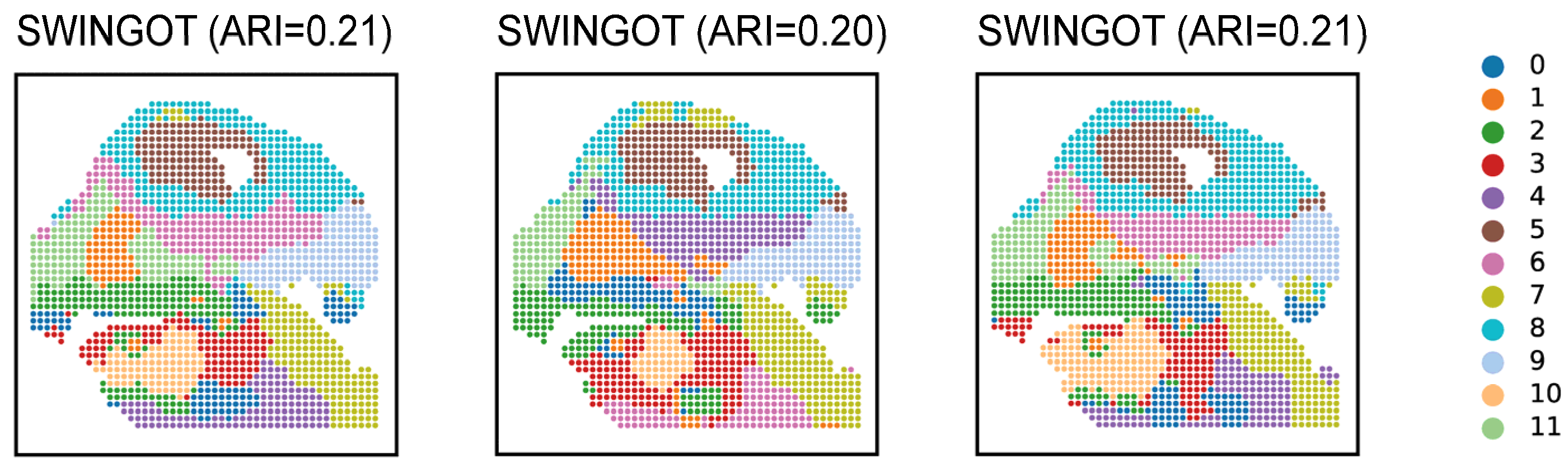
To examine the consistency of spatial-domain identification across different random initializations, we selected the E13 results obtained with three different random seeds and compared their spatial clustering maps (Figure A1). Each spot is colored according to the K-means clustering result (k = 12) on the fused representation. The corresponding ARI values were 0.21, 0.20, and 0.21, indicating similar agreement with the reference annotations. The maps also showed broadly similar spatial organization, although some local assignments and domain boundaries differed. These results suggest that the broad spatial patterns identified by SWINGOT were reasonably consistent across the three displayed runs.

Figure A1. Spatial-domain identification results obtained by SWINGOT across different runs on the E13 dataset. Each spot is colored according to the K-means clustering result (k = 12) on the fused representation. The corresponding ARI values are shown above the subplots.

Figure A1. Spatial-domain identification results obtained by SWINGOT across different runs on the E13 dataset. Each spot is colored according to the K-means clustering result (k = 12) on the fused representation. The corresponding ARI values are shown above the subplots.

Appendix A.5

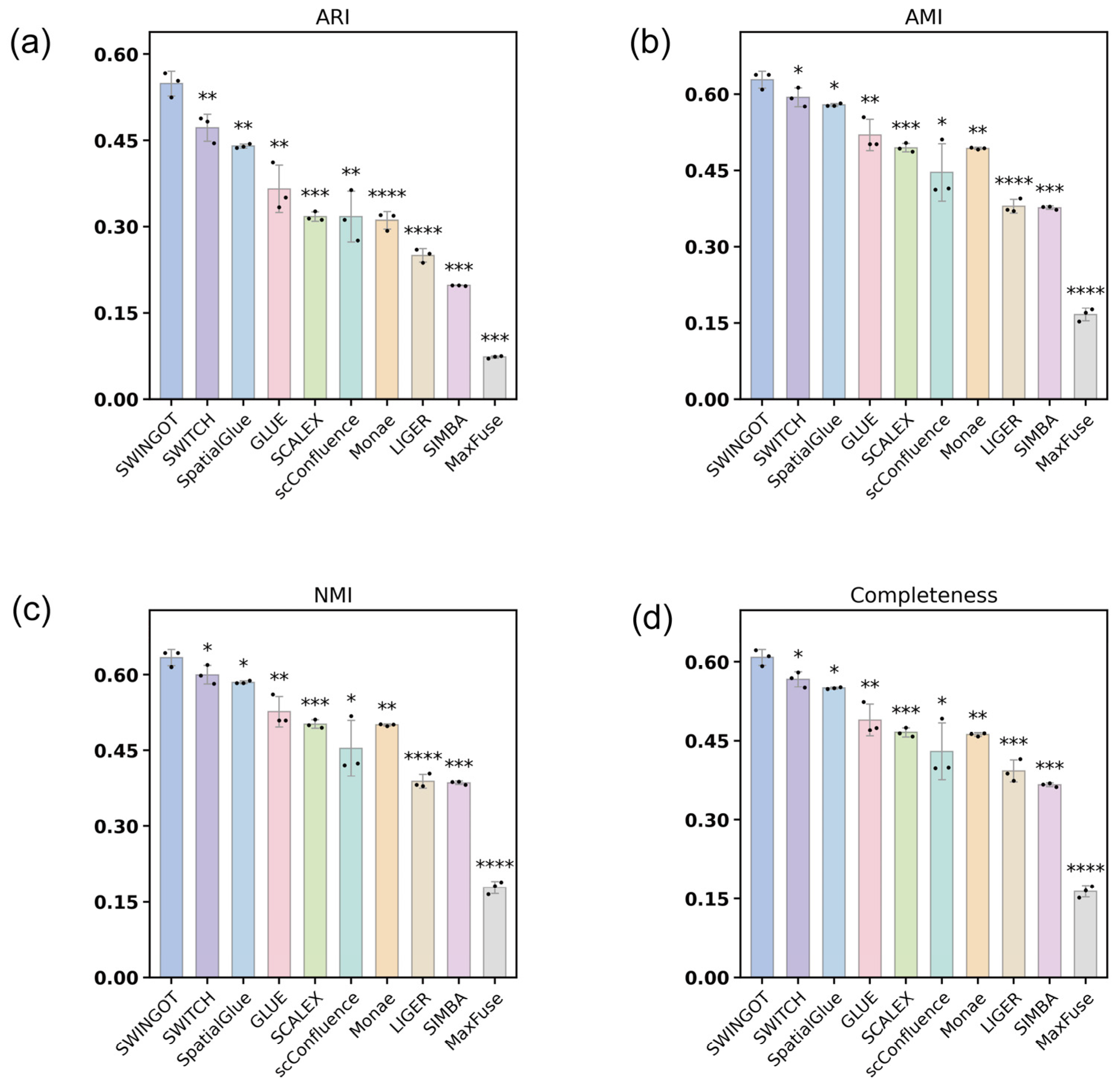
We performed additional comparisons on E15 using three random-seed runs per method (Figure A2). SWINGOT achieved the highest mean ARI, NMI, AMI, and Completeness among the compared methods. Pairwise comparisons between SWINGOT and each comparison method were performed using one-sided Welch two-sample tests, with the significance levels indicated in Figure A2.

Figure A2. Additional statistical comparisons on the E15 dataset. (a) ARI; (b) AMI; (c) NMI; and (d) Completeness. Each method was independently run with three random seeds. Bars show the means, error bars indicate standard deviations, and dots represent individual runs. Asterisks above each comparison method indicate its comparison with SWINGOT using a one-sided Welch two-sample t-test, with the alternative hypothesis that SWINGOT had a higher mean score. p values were not adjusted for multiple comparisons. Significance levels are indicated by one, two, three, and four asterisks for p < 0.05, p < 0.01, p < 0.001, and p < 0.0001, respectively.

Figure A2. Additional statistical comparisons on the E15 dataset. (a) ARI; (b) AMI; (c) NMI; and (d) Completeness. Each method was independently run with three random seeds. Bars show the means, error bars indicate standard deviations, and dots represent individual runs. Asterisks above each comparison method indicate its comparison with SWINGOT using a one-sided Welch two-sample t-test, with the alternative hypothesis that SWINGOT had a higher mean score. p values were not adjusted for multiple comparisons. Significance levels are indicated by one, two, three, and four asterisks for p < 0.05, p < 0.01, p < 0.001, and p < 0.0001, respectively.

Appendix A.6

We evaluated RNA reconstruction on E18 across 2000 highly variable genes. Expression was reconstructed through the modality-specific RNA encoder–decoder pathway and compared with the original expression and spatial smoothing, which averaged each spot with its six nearest spatial neighbors. Domain specificity was measured by η², the proportion of expression variance explained by the reference anatomical regions.

Figure A3. Evaluation of RNA reconstruction on E18 using 2000 highly variable genes. (a) Gene-wise Moran’s I. (b) Domain specificity (η²) based on reference anatomical annotations. (c) Gene-wise Moran’s I before and after reconstruction (Spearman ρ = 0.65). (d) Correlation with held-out RNA counts after count splitting. Bars show the mean of per-run median gene-wise Pearson correlations across three training seeds; error bars indicate standard deviations. PCA-50 denotes reconstruction with 50 principal components.

Figure A3. Evaluation of RNA reconstruction on E18 using 2000 highly variable genes. (a) Gene-wise Moran’s I. (b) Domain specificity (η²) based on reference anatomical annotations. (c) Gene-wise Moran’s I before and after reconstruction (Spearman ρ = 0.65). (d) Correlation with held-out RNA counts after count splitting. Bars show the mean of per-run median gene-wise Pearson correlations across three training seeds; error bars indicate standard deviations. PCA-50 denotes reconstruction with 50 principal components.

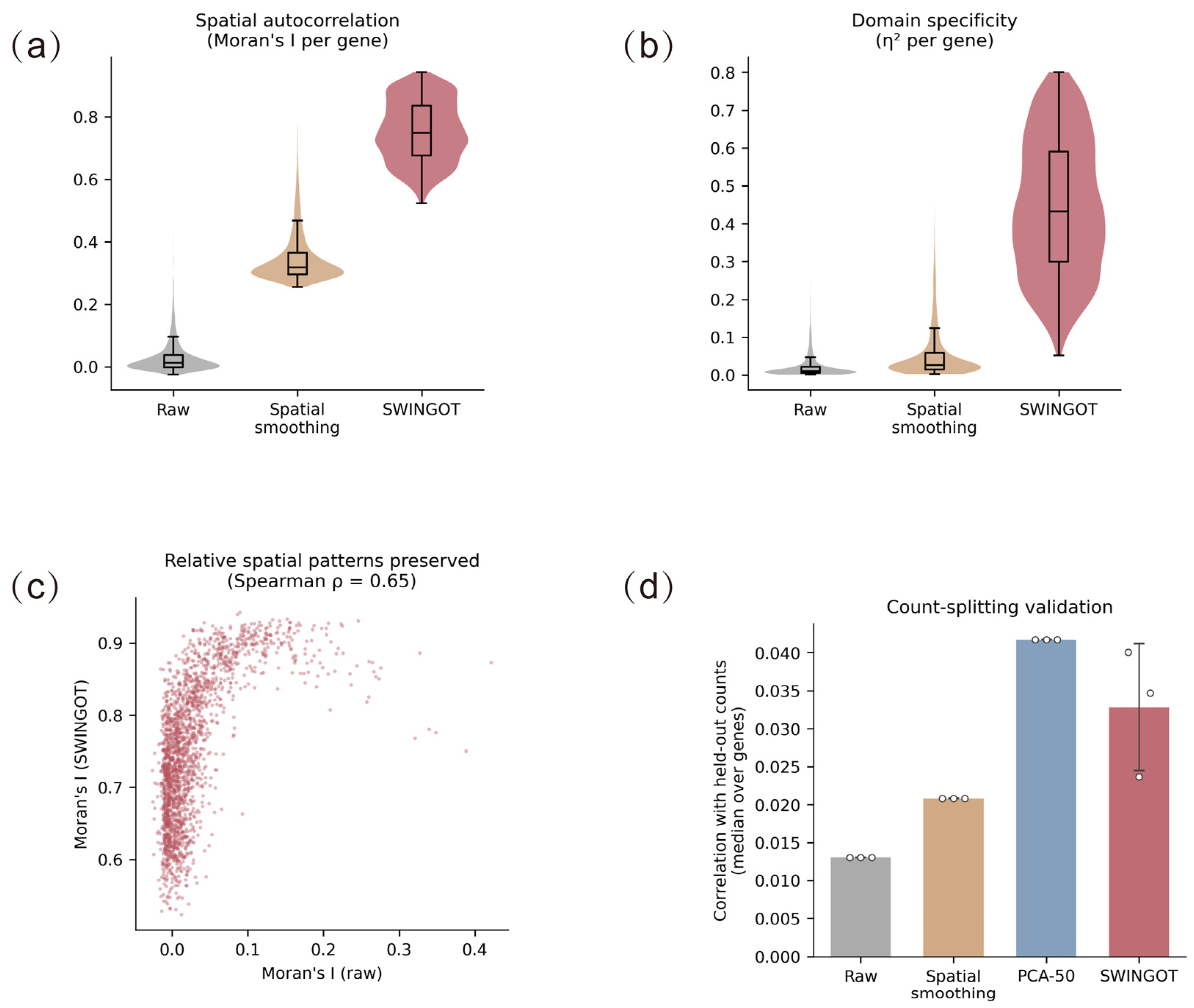
Median gene-wise Moran’s I was 0.012 for the original expression, 0.318 after spatial smoothing, and 0.749 after reconstruction (Figure A3a). The corresponding median η² values were 0.010, 0.027, and 0.432 (Figure A3b). Gene-wise, Moran’s I before and after reconstruction had a Spearman correlation of 0.65, indicating partial preservation of the relative ordering of spatial autocorrelation strength across genes (Figure A3c).

For count-splitting validation, original RNA counts were divided by binomial sampling into training and held-out portions. The model was fitted using the training portion and evaluated against the held-out counts. Across three training seeds, the mean of the per-run median gene-wise Pearson correlations was 0.033 ± 0.008 for SWINGOT. The corresponding values for the unreconstructed input, spatial smoothing, and PCA reconstruction with 50 components were 0.013, 0.021, and 0.042, respectively (Figure A3d).

References

- Zhang, L.; Chen, D.; Song, D.; Liu, X.; Zhang, Y.; Xu, X.; Wang, X. Clinical and Translational Values of Spatial Transcriptomics. Signal Transduct. Target. Ther. 2022, 7, 111. [Google Scholar] [CrossRef] [Scilit] [PubMed]
- Bressan, D.; Battistoni, G.; Hannon, G.J. The Dawn of Spatial Omics. Science 2023, 381, eabq4964. [Google Scholar] [CrossRef] [Scilit] [PubMed]
- Liu, X.; Peng, T.; Xu, M.; Lin, S.; Hu, B.; Chu, T.; Liu, B.; Xu, Y.; Ding, W.; Li, L.; et al. Spatial Multi-Omics: Deciphering Technological Landscape of Integration of Multi-Omics and Its Applications. J. Hematol. Oncol. 2024, 17, 72. [Google Scholar] [CrossRef] [Scilit] [PubMed]
- Carstens, J.L.; Krishnan, S.N.; Rao, A.; Sorace, A.G.; Seeley, E.H.; Ferri-Borgogno, S.; Burks, J.K. Spatial Multiplexing and Omics. Nat. Rev. Methods Primers 2024, 4, 54, Correction in Nat. Rev. Methods Primers 2024, 4, 65. https://doi.org/10.1038/s43586-024-00352-0. [Google Scholar] [CrossRef] [Scilit] [PubMed]
- Savitha, S.; Keerthana, R.; Logeswaran, K.; Keerthika, P.; Sharmila, V.; Sangeetha, M. Integration of Multi-Omics Data: Genomics, Proteomics, Metabolomics. In Harnessing AI and Machine Learning for Precision Wellness; IGI Global Scientific Publishing: Hershey, PA, USA, 2025; pp. 149–184. [Google Scholar]
- Polu, P.R. AI-Driven Chemometrics for Multi-Omics Data Integration: Advances, Challenges, and Future Directions. Crit. Rev. Anal. Chem. 2026, 1–36. [Google Scholar] [CrossRef] [Scilit] [PubMed]
- Sanghi, A.; Gruber, J.J.; Metwally, A.; Jiang, L.; Reynolds, W.; Sunwoo, J.; Orloff, L.; Chang, H.Y.; Kasowski, M.; Snyder, M.P. Chromatin Accessibility Associates with Protein-RNA Correlation in Human Cancer. Nat. Commun. 2021, 12, 5732. [Google Scholar] [CrossRef] [Scilit] [PubMed]
- Swindell, W.R.; Remmer, H.A.; Sarkar, M.K.; Xing, X.; Barnes, D.H.; Wolterink, L.; Voorhees, J.J.; Nair, R.P.; Johnston, A.; Elder, J.T.; et al. Proteogenomic Analysis of Psoriasis Reveals Discordant and Concordant Changes in mRNA and Protein Abundance. Genome Med. 2015, 7, 86. [Google Scholar] [CrossRef] [Scilit] [PubMed]
- Stahlschmidt, S.R.; Ulfenborg, B.; Synnergren, J. Multimodal Deep Learning for Biomedical Data Fusion: A Review. Brief. Bioinform. 2022, 23, bbab569. [Google Scholar] [CrossRef] [Scilit] [PubMed]
- Boehm, K.M.; Khosravi, P.; Vanguri, R.; Gao, J.; Shah, S.P. Harnessing Multimodal Data Integration to Advance Precision Oncology. Nat. Rev. Cancer 2022, 22, 114–126. [Google Scholar] [CrossRef] [Scilit] [PubMed]
- Welch, J.D.; Kozareva, V.; Ferreira, A.; Vanderburg, C.; Martin, C.; Macosko, E.Z. Single-Cell Multi-Omic Integration Compares and Contrasts Features of Brain Cell Identity. Cell 2019, 177, 1873–1887.e17. [Google Scholar] [CrossRef] [Scilit] [PubMed]
- Xiong, L.; Tian, K.; Li, Y.; Ning, W.; Gao, X.; Zhang, Q.C. Online Single-Cell Data Integration through Projecting Heterogeneous Datasets into a Common Cell-Embedding Space. Nat. Commun. 2022, 13, 6118. [Google Scholar] [CrossRef] [Scilit] [PubMed]
- Cao, Z.-J.; Gao, G. Multi-Omics Single-Cell Data Integration and Regulatory Inference with Graph-Linked Embedding. Nat. Biotechnol. 2022, 40, 1458–1466. [Google Scholar] [CrossRef] [Scilit] [PubMed]
- Chen, H.; Ryu, J.; Vinyard, M.E.; Lerer, A.; Pinello, L. SIMBA: Single-Cell Embedding along with Features. Nat. Methods 2024, 21, 1003–1013. [Google Scholar] [CrossRef] [Scilit] [PubMed]
- Chen, S.; Zhu, B.; Huang, S.; Hickey, J.W.; Lin, K.Z.; Snyder, M.; Greenleaf, W.J.; Nolan, G.P.; Zhang, N.R.; Ma, Z. Integration of Spatial and Single-Cell Data across Modalities with Weakly Linked Features. Nat. Biotechnol. 2024, 42, 1096–1106. [Google Scholar] [CrossRef] [Scilit] [PubMed]
- Samaran, J.; Peyré, G.; Cantini, L. scConfluence: Single-Cell Diagonal Integration with Regularized Inverse Optimal Transport on Weakly Connected Features. Nat. Commun. 2024, 15, 7762. [Google Scholar] [CrossRef] [Scilit] [PubMed]
- Tang, Z.; Chen, G.; Chen, S.; Yao, J.; You, L.; Chen, C.Y.-C. Modal-Nexus Auto-Encoder for Multi-Modality Cellular Data Integration and Imputation. Nat. Commun. 2024, 15, 9021. [Google Scholar] [CrossRef] [Scilit] [PubMed]
- Du, Y.; Fan, K.; Lu, X.; Wu, C. Integrating Multi–Omics Data for Gene-Environment Interactions. BioTech 2021, 10, 3. [Google Scholar] [CrossRef] [Scilit] [PubMed]
- Yoshikawa, T.; Bülow, R.D.; Boor, P.; Yanagita, M. Next-Generation Kidney Tissue Analysis—Spatial Omics and Digital Pathology. Nat. Rev. Nephrol. 2026, 22, 603–621. [Google Scholar] [CrossRef] [Scilit] [PubMed]
- Dong, K.; Zhang, S. Deciphering Spatial Domains from Spatially Resolved Transcriptomics with an Adaptive Graph Attention Auto-Encoder. Nat. Commun. 2022, 13, 1739. [Google Scholar] [CrossRef] [Scilit] [PubMed]
- Li, Z.; Qu, S.; Liang, H.; Tang, R.; Zhang, X.; Lu, F.; Yang, J.; Gan, Z.; Gao, S.; Zhang, Y.; et al. Integrative Deep Learning of Spatial Multi-Omics with SWITCH. Nat. Comput. Sci. 2025, 5, 1051–1063. [Google Scholar] [CrossRef] [Scilit] [PubMed]
- Yu, L.; Ma, T.; Zhao, W.; Liang, Z.; Yu, L. MoST-IG: Morphology-Guided Spatial Transcriptomics Integration via Visual-Genomic Graph Optimal Transport. In Proceedings of the Medical Image Computing and Computer Assisted Intervention–MICCAI 2025; Gee, J.C., Alexander, D.C., Hong, J., Iglesias, J.E., Sudre, C.H., Venkataraman, A., Golland, P., Kim, J.H., Park, J., Eds.; Springer Nature: Cham, Switzerland, 2026; pp. 490–499. [Google Scholar]
- Jiang, F.; Zhou, X.; Qian, Y.; Zhu, M.; Wang, L.; Li, Z.; Shen, Q.; Wang, M.; Qu, F.; Cui, G.; et al. Simultaneous Profiling of Spatial Gene Expression and Chromatin Accessibility during Mouse Brain Development. Nat. Methods 2023, 20, 1048–1057. [Google Scholar] [CrossRef] [Scilit] [PubMed]
- Long, Y.; Ang, K.S.; Sethi, R.; Liao, S.; Heng, Y.; van Olst, L.; Ye, S.; Zhong, C.; Xu, H.; Zhang, D.; et al. Deciphering Spatial Domains from Spatial Multi-Omics with SpatialGlue. Nat. Methods 2024, 21, 1658–1667. [Google Scholar] [CrossRef] [Scilit] [PubMed]
Disclaimer/Publisher’s Note: The statements, opinions and data contained in all publications are solely those of the individual author(s) and contributor(s) and not of MDPI and/or the editor(s). MDPI and/or the editor(s) disclaim responsibility for any injury to people or property resulting from any ideas, methods, instructions or products referred to in the content. |
© 2026 by the authors. Licensee MDPI, Basel, Switzerland. This article is an open access article distributed under the terms and conditions of the Creative Commons Attribution (CC BY) license.