


Abstract
Rice blast, caused by Magnaporthe oryzae, is a devastating fungal disease threatening global rice production, with annual yield losses ranging from 10% to 30% in epidemic regions. Conventional detection methods rely on visual inspection and laboratory diagnosis, which are limited by subjectivity, time-consuming procedures, and the inability to detect early-stage infections. Hyperspectral imaging technology offers a highly promising method for detecting rice blast disease. It can capture the physiological and biochemical changes that occur in plant tissues before the appearance of visible symptoms. In this study, we propose a Convolutional-State Space Hybrid Network (CS-HybridNet) featuring a dual-branch deep learning architecture that synergistically combines a ConvNeXt-based spatial branch with a LiteMamba-based global spatial branch (which models long-range spatial dependencies with spectral embeddings). Principal component analysis was employed to reduce the dimensionality from 360 hyperspectral bands to 16 principal components, retaining 99.09% of the original information while significantly improving computational efficiency. An adaptive feature fusion module effectively integrates spatial texture features with spectral features, enabling complementary information utilization. Experimental results on a dataset comprising 166 hyperspectral images demonstrate that CS-HybridNet achieves 96.30% ± 1.38% accuracy, 98.33% precision, 95.16% recall, and an AUC–ROC value of 0.971 on the independent test set, outperforming traditional machine learning methods and existing deep learning models by 3.5–12.8% in accuracy. Ablation studies validate the effectiveness of each component. This research demonstrates the efficacy of spatial-spectral fusion architecture for automated plant disease detection and establishes a technical foundation for the development of intelligent crop disease monitoring systems.
1. Introduction
Rice (Oryza sativa L.) is one of the most important food crops globally, with global rice production reaching 787 million tons in 2023, feeding more than half of the world’s population [1,2]. Rice blast disease, caused by the ascomycete fungus Magnaporthe oryzae, is one of the most destructive fungal diseases in rice production. It occurs in more than 85 rice-growing countries and regions worldwide, causing annual yield losses of 10–30%, equivalent to food sufficient to feed 60 million people [3,4,5]. The pathogen exhibits high genetic variability and environmental adaptability, often causing resistant varieties to lose their resistance within a few years of deployment [6,7]. Therefore, developing non-destructive, rapid, and accurate early detection technologies for rice blast disease is of great significance for guiding precision pesticide application and reducing yield losses. Beyond immediate disease management, automated and high-throughput detection technologies can provide technical support for rice blast resistance breeding programs. High-throughput phenotyping using hyperspectral imaging may facilitate screening breeding populations for resistance genes, assessing resistance across genetic backgrounds, and phenotypic evaluation of candidate genes from GWAS or QTL mapping. Such automated detection systems have the potential to alleviate the scalability challenges of traditional visual assessment in genomic-assisted breeding.
Traditional rice blast disease detection methods primarily rely on field visual inspection and laboratory pathogen identification [8,9]. Although visual inspection is cost-effective, it heavily depends on the experience level of plant protection personnel, is highly subjective, and by the time disease symptoms become visible, the pathogen has often completed extensive reproduction and begun to spread [10]. Laboratory diagnostic methods such as PCR technology offer high accuracy but have long detection cycles and high costs, failing to meet the needs of large-scale, rapid screening [11]. Therefore, there is an urgent need to develop novel rapid-detection technologies to enable early warning and precision control of rice blast disease.
Hyperspectral imaging technology integrates the advantages of spectroscopy and imaging techniques, enabling simultaneous acquisition of spatial and spectral information of target objects [12,13]. Unlike traditional RGB imaging technology, hyperspectral imaging systems can continuously acquire spectral reflectance data across hundreds of narrow bands in the 400–2500 nm wavelength range, forming three-dimensional data cubes containing rich spectral-spatial information [14,15]. This characteristic enables the detection of subtle changes in physiological and biochemical parameters, such as tissue structure, pigment content, and moisture status, after plant infection, even during the latent period when disease symptoms have not yet appeared [16,17]. Studies have shown that Rice blast infection causes distinctive physiological changes in leaf tissue that manifest as spectral reflectance patterns. Magnaporthe oryzae infection disrupts chloroplast structure and reduces chlorophyll content, leading to decreased absorption in the visible spectrum (particularly around 680 nm). Cell membrane damage and altered water relations affect near-infrared reflectance (750–1300 nm). These biochemical and structural changes create detectable spectral signatures even before visible symptoms emerge, providing the physiological basis for hyperspectral disease detection [18,19].
In recent years, hyperspectral imaging technology has made significant progress in plant disease detection. Zhang et al. [20] proposed a hyperspectral imaging-based method for early detection of tomato bacterial leaf spot disease, achieving disease identification at the pre-symptomatic stage and demonstrating the great potential of hyperspectral technology for early disease detection. Ram et al. [21] conducted a systematic review of hyperspectral imaging applications in precision agriculture from 2020–2024, indicating exponential growth in the detection of crop diseases, nutrient deficiencies, and environmental stresses. Cheshkova [22] proposed a comprehensive framework for plant disease diagnosis based on hyperspectral analysis, systematically summarizing key steps in image acquisition, feature extraction, and model analysis. However, traditional methods primarily rely on manual feature extraction and shallow machine learning models, suffering from complex feature engineering, limited generalization capability, and difficulty in fully exploiting deep spatial-spectral joint features in hyperspectral data [23,24].
Deep learning, through constructing multi-layer neural network models, can automatically learn hierarchical feature representations from raw data, achieving revolutionary breakthroughs in computer vision [25,26]. Convolutional neural networks (CNNs), with their powerful spatial feature extraction capabilities, have become the mainstream architecture for image recognition tasks [27,28]. ResNet, proposed by He et al. [29], addressed the gradient vanishing problem in deep networks through residual connections, laying the foundation for subsequent deep network development. In crop disease detection applications, deep learning methods have shown great potential. Liang et al. [30] proposed a deep convolutional neural network-based rice blast disease recognition method, achieving over 95% accuracy on large-scale datasets. Shah et al. [31] compared the performance of multiple deep learning architectures in early rice disease detection, validating the effectiveness of deep learning methods. Recent reviews [32,33] systematically analyzed the development trends in deep learning for rice disease identification, indicating that lightweight models and multi-scale feature extraction are important research directions. Cao et al. [34] proposed the Pyramid-YOLOv8 model, achieving precise real-time detection of rice blast leaf lesions via a multi-attention feature fusion network, achieving an mAP of 84.3%. However, standard 2D CNNs are primarily designed for RGB images and have limitations when processing high-dimensional hyperspectral data [35].
To address this, Chen et al. [36] proposed a 3D CNN architecture that performs convolution operations simultaneously across the spatial and spectral dimensions using 3D convolution kernels, providing new insights for hyperspectral image classification. Roy et al. [37] designed the HybridSN network, innovatively combining 3D and 2D convolutions to extract spatial-spectral features, achieving strong performance on multiple benchmark datasets. Ahmad et al. [38] developed a fast and compact 3D CNN model that significantly reduced computational complexity while maintaining high classification accuracy. Recent studies [39,40] further explored hybrid 2D-3D CNN architectures and depthwise separable convolution techniques to improve model computational and parameter efficiency. Despite certain achievements of 3D CNNs, their parameter count and computational complexity increase significantly, making them prone to overfitting under small-sample conditions [41].
The proposal of the Transformer architecture introduced revolutionary changes to sequence modeling tasks, with its core self-attention mechanism capable of capturing long-range dependencies between sequence elements [42]. Vision Transformer (ViT), proposed by Dosovitskiy et al. [43], divides images into fixed-size patch sequences and uses self-attention mechanisms to model global relationships, achieving performance comparable to or better than CNNs in image classification tasks. In the field of hyperspectral image classification, Transformer architectures have also been widely applied. Hong et al. [44] proposed SpectralFormer, revisiting hyperspectral image classification from a sequence modeling perspective and achieving efficient spectral-spatial feature extraction by learning grouped spectral embeddings of adjacent bands. Sun et al. [45] proposed the Spectral-Spatial Feature Tokenization Transformer (SSFT), achieving state-of-the-art performance on multiple benchmark datasets by converting hyperspectral cubes into a series of spectral-spatial tokens. Roy et al. [46] developed the Morphological Attention Transformer (MorphFormer), combining trainable morphological operations to enhance spatial-spectral feature interaction. Recent studies [47,48] further explored hybrid convolution-Transformer architectures and multi-scale feature fusion strategies to better utilize spatial-spectral information in hyperspectral data. Scheibenreif et al. [49] proposed masked vision Transformers for hyperspectral image classification, improving model generalization in few-shot scenarios through self-supervised pre-training. However, Transformer architectures suffer from quadratic computational complexity and dependence on large-scale training data, facing challenges in agricultural applications where labeled samples are limited [50,51].
Recently, State Space Models (SSMs) have shown great potential in sequence modeling and visual tasks. The Mamba architecture proposed by Gu et al. [52] achieves significant reduction in computational cost through selective state space mechanisms and linear complexity design while maintaining long-range dependency modeling capability, providing an efficient solution for processing long sequence data. Zhu et al. [53] introduced Mamba to the visual domain, proposing the Vision Mamba (Vim) architecture, which processes image sequences through bidirectional state space models, achieving higher performance and efficiency than Vision Transformer on tasks including ImageNet classification, COCO object detection, and ADE20K semantic segmentation, with 2.8× speed improvement and 86.8% GPU memory savings in feature extraction for 1248 × 1248 resolution images. Liu et al. [54] proposed VMamba, using cross-scan modules to enhance the global receptive field of visual state space models, further improving model performance. A recent review [55] systematically summarized the evolution from traditional methods to Transformer and Mamba models in hyperspectral image classification, indicating that Mamba has achieved significant breakthroughs in long-sequence modeling tasks, providing new technical pathways for hyperspectral data processing. However, the application of Mamba in hyperspectral image analysis is still in its infancy, and how to effectively combine it with CNN architectures to fully leverage the advantages of both remains an open question.
Meanwhile, ConvNeXt proposed by Liu et al. [56], as a modernized pure convolutional network architecture, significantly improved performance by borrowing design concepts from Transformers (such as large convolution kernels, depthwise separable convolutions, layer normalization, etc.) while maintaining the inductive bias advantages of convolutional networks, achieving 87.8% accuracy on ImageNet classification and outperforming Swin Transformer on COCO detection and ADE20K segmentation tasks. Woo et al. [57] further proposed ConvNeXt V2, introducing a fully convolutional masked autoencoder framework (FCMAE) and Global Response Normalization (GRN) layers, significantly improving the performance of pure convolutional networks across various recognition benchmarks through the synergistic design of self-supervised learning techniques and architectural improvements, from efficient 3.7 M parameter Atto models to 650 M parameter Huge models (ImageNet accuracy 88.9%), demonstrating strong scalability. The success of the ConvNeXt architecture indicates that well-designed convolutional networks remain highly competitive, particularly for tasks that require spatial locality and inductive bias preservation.
Despite certain progress in hyperspectral disease detection, the following key scientific challenges remain: First, insufficient decoupling and synergistic utilization of spatial-spectral features, as existing methods mostly adopt single-branch architectures, making it difficult to simultaneously exploit spatial texture patterns and spectral information in hyperspectral data [58,59]. Second, the curse of dimensionality and computational efficiency bottlenecks caused by high-dimensional spectral data [60,61,62,63]; Third, challenges in model generalization under small-sample conditions [64]. These limitations highlight the need for developing dual-branch architectures that can effectively decouple and synergistically utilize spatial-spectral features while maintaining computational efficiency and generalization capability under limited training samples.
Based on the above analysis, this study proposes a Convolutional-State Space Hybrid Network (CS-HybridNet) for high-accuracy automatic detection of rice blast disease. Addressing the three key challenges mentioned above, the main innovations of this study include:
- (1)
- Addressing the problem of spatial-spectral feature decoupling and synergistic utilization, an innovative ConvNeXt–LiteMamba dual-branch architecture is proposed, which achieves high computational efficiency (45 M parameters, 8.20 GFLOPs, and 15 ms inference time). The ConvNeXt spatial branch extracts local spatial morphological features through hierarchical convolutions with limited receptive fields, while the LiteMamba branch models long-range spatial dependencies across the image, with each spatial token encoded by 16-dimensional spectral features. This design captures global spatial context while incorporating spectral information through token embeddings, complementing ConvNeXt’s local spatial feature extraction. LiteMamba reduces the parameter count and computational overhead by simplifying the selective state space mechanism of the original Mamba while maintaining linear time complexity, making it more suitable for small-sample hyperspectral scenarios. An Adaptive Feature Fusion Module (AFFM) is further designed to achieve deep interaction of heterogeneous features through learnable projection layers and nonlinear transformations.
- (2)
- Addressing the curse of dimensionality in high-dimensional spectral data, a PCA-based intelligent dimensionality reduction strategy is proposed, reducing 360 bands to 16 principal components, achieving an 18× improvement in inference speed while retaining 99.09% of the original information. An end-to-end learnable RGB mapping mechanism is designed to adaptively extract the most discriminative pseudo-RGB channels from principal components through a Softmax-normalized weight matrix.
- (3)
- Addressing the generalization challenge under small-sample conditions (166 hyperspectral images), the complementary information from the dual-branch architecture is fully utilized to enhance sample representation capability. PCA dimensionality reduction achieves denoising and regularization effects while preserving discriminative information. ConvNeXt with strong inductive bias and the lightweight LiteMamba architecture are selected instead of Transformers that depend on large data, designed to address the challenge of maintaining detection accuracy under small-sample conditions and to achieve competitive performance compared to attention-based methods.
- (4)
- Comprehensive experimental validation was conducted on a self-built rice blast hyperspectral dataset. Ablation experiments quantified the contributions of the dual-branch architecture and adaptive fusion. Comparative experiments demonstrated significant advantages over 8 existing methods. Feature visualization revealed the internal working mechanisms of the model, providing new methodological references for the development of hyperspectral disease-detection technology.
2. Materials and Methods
2.1. Data Acquisition and Preprocessing
Data acquisition was conducted over approximately 9 collection days spanning from early May to early July 2025, corresponding to three growth stages of early-season rice. Specifically, seedling-stage samples were collected during early to mid-May 2025, tillering-stage samples during early to mid-June 2025, and jointing-stage samples during late June to early July 2025. Data acquisition was conducted in the experimental rice fields at Hunan Agricultural University, Changsha, China. All hyperspectral images were captured using a single push-broom hyperspectral camera. Data collection was scheduled daily between 9:00 AM and 4:00 PM to ensure sufficient and stable natural illumination. Rice samples were collected as whole plants from the field. To maintain their physiological vitality during transport, the root systems were carefully kept with their surrounding rhizosphere soil intact and were then wrapped with moist preservation material to retain humidity. All samples were transported to the laboratory within 60 min post-collection. Hyperspectral imaging of each sample was completed within 2 h after collection to minimize physiological changes and ensure data quality.
Experimental samples were collected from rice plants naturally infected with blast disease in the field and from healthy control plants at different growth stages from seedling to jointing. Sample labeling was performed by two experienced plant protection experts using visual symptom assessment based on standardized rice blast disease grading scales. Diseased samples exhibited visible lesions characteristic of rice blast (diamond-shaped or elliptical lesions with gray-white centers and brown margins). Healthy samples showed no visible disease symptoms.
The hyperspectral imaging system was configured with a push-broom line-scan camera, continuously acquiring 360 spectral bands in the 400–2500 nm wavelength range with a spectral resolution of approximately 5.8 nm. Radiometric calibration was performed using a white reference panel before acquiring hyperspectral images. Raw data was stored in 16-bit format and converted to reflectance after dark current correction. The raw hyperspectral images (3680 × 560 pixels) containing approximately 6 rice plants were processed using a custom Python script with the following procedure: First, the .raw and .hdr file pairs were parsed using spectral imaging libraries. Then, the large images were segmented into rectangular sections using a fixed grid approach. Each segmented section containing an individual rice plant was resampled to 224 × 224 pixels using band-by-band bilinear interpolation. The disease status (healthy or diseased) was automatically assigned based on the source folder naming convention, with expert verification of all labels. Figure 1 presents the hyperspectral data acquisition system and representative sample images. Figure 1a provides a schematic diagram of the laboratory imaging setup, illustrating the spatial arrangement of the push-broom camera, halogen light sources, motorized translation stage, and the white reference panel calibration procedure. Figure 1b depicts the field sampling and sample preparation workflow, from rice plant collection in the experimental field through sample preservation and transport to laboratory delivery for hyperspectral imaging. Figure 1c shows representative true-color hyperspectral images of rice leaves at different health states: (i) healthy sample, (ii) early-stage infected sample, and (iii) late-stage infected sample. Min-max normalization was then applied to standardize reflectance values to the [0, 1] range:
where represents the raw hyperspectral data tensor. To prevent data leakage in preprocessing, min-max normalization parameters (minimum and maximum values) were computed exclusively from training set samples and subsequently applied to validation and test sets using the same parameters. PCA was fitted only to training-set pixels, and the resulting projection matrix W was then applied to transform the validation and test sets. Table 1 lists the key technical parameters for hyperspectral data acquisition.
Figure 1.
Hyperspectral data acquisition system and representative sample images. (a) Laboratory imaging setup schematic. (b) Field sampling and sample preparation workflow. (c) Representative true-color images: (i) healthy, (ii) early-infection, and (iii) late-infection samples.
Table 1.
Hyperspectral data acquisition parameters.
After quality screening and expert review, this study ultimately constructed a dataset containing 166 hyperspectral images, including 61 healthy samples (36.7%) and 105 diseased samples (63.3%). The dataset was divided into training, validation, and test subsets using stratified random sampling, ensuring that the proportions of healthy and diseased samples in each subset remained consistent with the overall dataset. Table 2 presents the detailed statistics for each subset.
Table 2.
Dataset split statistics.
To enhance model generalization and mitigate overfitting under small-sample conditions, various data augmentation strategies were applied to training set samples during the training phase. Specifically: (1) random horizontal flip (probability 0.5) and random vertical flip (probability 0.5) to simulate different leaf orientations; (2) random rotation (within ±15° range) to increase sample angular diversity; (3) random brightness adjustment (within ±10% range) and random contrast adjustment (within ±10% range) to simulate different lighting conditions. These augmentation operations were randomly applied during each training epoch, effectively expanding the diversity of training samples. No data augmentation was applied to the validation and test sets to ensure objectivity and comparability of evaluation results.
The 360 spectral bands contained in hyperspectral images introduce the curse of dimensionality and computational redundancy. This study employed Principal Component Analysis (PCA) for spectral dimensionality reduction. PCA was performed on per-pixel spectra pooled from all training images. Specifically, each pixel’s 360-dimensional spectral vector was treated as an independent sample, yielding approximately 5.8 million pixel samples (115 images × 224 × 224 pixels) for PCA fitting. This pixel-level approach is justified by two considerations: (1) hyperspectral disease detection fundamentally relies on pixel-level spectral features, as disease symptoms manifest as localized spectral changes in affected tissue regions; (2) aggregating at the image level would blur the within-image spectral variability necessary for identifying localized lesions, thereby losing fine-grained discriminative information critical for early disease detection.
Let the original hyperspectral data matrix be , where N is the number of pixel samples, and D is the original dimensionality (360 bands). First, the data was centered:
Then the covariance matrix was computed, and eigenvalue decomposition was performed:
where is a diagonal matrix with eigenvalues arranged in descending order on the diagonal. The eigenvectors corresponding to the top k largest eigenvalues were selected to form the projection matrix , projecting the original data onto the k-dimensional principal component space. The number of principal components k was determined by the cumulative explained variance ratio:
The number of principal components k was determined through preliminary experiments comparing k = {8, 16, 32, 64}, with k = 16 selected based on the balance between accuracy and computational efficiency (detailed analysis in Section 3.4). Given the large data volume, incremental PCA was employed for computation, iteratively fitting with batches of 10,000 pixels. After dimensionality reduction, the data dimensions were transformed from to . Figure 2 presents a schematic diagram of the complete data preprocessing pipeline, illustrating the workflow from raw hyperspectral image acquisition through normalization, PCA dimensionality reduction, and data augmentation to the final model input.
Figure 2.
Schematic diagram of data preprocessing pipeline.
2.2. Model Architecture Design
The Convolutional-State Space Hybrid Network (CS-HybridNet) proposed in this study adopts a dual-branch parallel architecture, aiming to fully exploit spatial and spectral features in hyperspectral images and achieve synergistic utilization of both types of information through an adaptive fusion mechanism. Figure 3 illustrates the complete architecture of CS-HybridNet.
Figure 3.
Complete architecture diagram of CS-HybridNet.
The PCA-reduced hyperspectral data (dimensions , where B is batch size) simultaneously enter the spatial and spectral branches for parallel processing. The spatial branch, based on ConvNeXt architecture, is specifically designed to extract spatial texture features and morphological patterns from images. The LiteMamba branch models long-range spatial dependencies across the image, with each spatial token encoded by 16-dimensional spectral features. This design captures global spatial context while incorporating spectral information through token embeddings, complementing ConvNeXt’s local spatial feature extraction. LiteMamba is a lightweight state space model optimized for small-sample hyperspectral scenarios, reducing parameter overhead while maintaining linear complexity by simplifying the original Mamba architecture. The output features from both branches are integrated through the Adaptive Feature Fusion Module and finally fed into a binary classifier for disease discrimination.
2.2.1. ConvNeXt Spatial Branch
The spatial branch first projects the 16 spectral channels into a 3-channel pseudo-color image through a learnable RGB mapping layer. This mapping employs an end-to-end learnable weighted fusion mechanism, expressed mathematically as
where represents the i-th RGB channel (); represents the j-th spectral channel; and are learnable weight parameters. The weight matrix is normalized through Softmax to ensure weighted fusion of all spectral bands for each RGB channel:
where are learnable parameters. The data dimensions after RGB mapping are transformed to . This design automatically determines optimal band combination strategies through end-to-end learning, enabling the model to adaptively extract the most discriminative spatial features from hyperspectral data.
The RGB-mapped data passes through the Stem layer for preliminary feature extraction and spatial downsampling. The Stem layer employs a convolution kernel with stride 4, reducing spatial resolution from to while expanding the channel count to 96 dimensions.
The ConvNeXt Block is the basic building unit of the spatial branch, designed by drawing on successful experiences from Transformers while retaining the inductive bias advantages of convolutional networks. The forward propagation of a single ConvNeXt Block can be expressed as:
where is a learnable layer scaling parameter, initialized to a small value (e.g., ), used to stabilize training of deep networks. The layer scaling parameter is a learnable per-channel vector. This design, introduced by Liu et al. [56], serves to stabilize the training of deep networks by initially allowing residual connections to dominate, then gradually increasing the contribution of the transformed features as training progresses. The element-wise multiplication scales each channel independently, providing fine-grained control over feature contributions. The depthwise separable convolution provides a large receptive field, capable of capturing broader spatial context information. The GELU activation function has smoother gradient characteristics compared to ReLU. DropPath serves as an effective regularization technique by randomly dropping entire residual paths.
The ConvNeXt spatial branch comprises 4 stages, each consisting of multiple stacked ConvNeXt Blocks. The specific configuration is: Stage 1 contains 3 Blocks (96 channels), Stage 2 contains 3 Blocks (192 channels), Stage 3 contains 9 Blocks (384 channels), and Stage 4 contains 3 Blocks (768 channels). Between stages, downsampling layers ( convolution, stride 2) halve the spatial resolution and double the channel count. Finally, the output feature maps from Stage 4 undergo global average pooling to generate a 768-dimensional global spatial feature vector:
Figure 4 illustrates the internal structure of the ConvNeXt Block in detail. This module achieves efficient spatial feature extraction through 7 × 7 depthwise separable convolution, layer normalization, inverted bottleneck structure, GELU activation, layer scaling, and residual connections.
Figure 4.
ConvNeXt block architecture of the spatial branch.
2.2.2. LiteMamba Branch
This study proposes the LiteMamba architecture, optimized for small-sample hyperspectral scenarios. Compared to traditional Transformers, LiteMamba is based on state space models with linear time complexity, enabling more efficient processing of long sequence data. Compared to the original Mamba architecture, LiteMamba significantly reduces parameter count and computational overhead while maintaining long-range dependency modeling capability by simplifying the state selection mechanism. The LiteMamba branch models long-range spatial dependencies across the image, with each spatial token encoded by 16-dimensional spectral features. This design captures global spatial context while incorporating spectral information through token embeddings, complementing ConvNeXt’s local spatial feature extraction. LiteMamba retains the core designs of gating mechanisms and depthwise convolution, significantly reducing parameter count and computational overhead by removing the complex selective state-space mechanism from the original Mamba while maintaining linear-time complexity. These modifications reduce parameter count by approximately 70% while lowering the risk of overfitting on small-scale datasets. LiteMamba was adopted because the original Mamba’s parameter count may cause overfitting on the small-scale dataset of 166 samples. Ablation experiments demonstrate that the simplified version improves generalization while maintaining modeling capability.
First, adaptive spatial pooling is applied to reduce spatial resolution from to , reducing the computational burden of subsequent sequence processing:
Subsequently, the spatial dimensions are flattened into sequence form
where the sequence length , with each position corresponding to a pixel in space containing 16-dimensional spectral information.
The sequentialized spectral data passes through a spectral embedding layer for dimension expansion, mapping the 16-dimensional original spectral features to a 256-dimensional high-dimensional embedding space:
where is the learnable spectral embedding matrix that projects the 16-dimensional PCA spectral features to a 256-dimensional high-dimensional embedding space. This projection enables the model to learn richer spectral representations suitable for subsequent sequence modeling.
Learnable positional encodings are simultaneously introduced to preserve sequence positional information:
where is the learnable positional encoding matrix, initialized with a normal distribution (std = 0.02).
The core component of the spectral branch is the LiteMamba Block. This module retains the core designs of gating mechanisms and depthwise convolution, significantly reducing parameter count and computational overhead by removing the complex selective state-space mechanism from the original Mamba while maintaining linear-time complexity. This simplified design makes LiteMamba better suited to hyperspectral sequence modeling under small-sample conditions, reducing the risk of overfitting caused by over-parameterization. The forward propagation of each LiteMamba Block can be expressed as
where is the expansion dimension, and Conv1d employs a 1D convolution with kernel size 4 to capture local dependencies along the spatial token sequence. The gating mechanism (⊙ denotes element-wise multiplication) adaptively controls information flow, enhancing model expressiveness.
The spectral branch consists of 6 sequentially stacked LiteMamba Blocks with the following configuration parameters: hidden dimension 256, state dimension 16, convolution kernel size 4, and expansion factor 2. Finally, global average pooling generates a 256-dimensional global spectral feature:
Figure 5 illustrates the internal structure of the LiteMamba Block in detail. This module processes spatial token sequences where each token contains spectral embeddings, achieving efficient modeling of global spatial dependencies while maintaining linear time complexity through input projection and branching, 1D convolution, a gating mechanism, output projection, and residual connections. Compared to the original Mamba, LiteMamba reduces parameter count by approximately 70% by removing the complex selective state space mechanism, making it more suitable for small-sample hyperspectral scenarios.
Figure 5.
LiteMamba block architecture of the spectral branch.
2.2.3. Adaptive Feature Fusion Module
The Adaptive Feature Fusion Module (AFFM) is responsible for integrating complementary features extracted by the spatial and spectral branches. Since the two branches output features with different dimensions (spatial features 768-dimensional, spectral features 256-dimensional), direct concatenation would result in high-dimensional features dominating the fused result. Therefore, AFFM first projects both feature types into a unified 256-dimensional space through projection layers, then performs concatenation and deep fusion.
Spatial feature projection:
where is the learnable projection matrix.
Spectral feature projection:
where is the learnable projection matrix.
Feature concatenation:
Fusion layer processing:
AFFM achieves better feature integration than simple concatenation through dimension alignment and deep fusion. The total parameter count for the module is approximately 0.53 M, including the spatial projection layer (0.20 M), the spectral projection layer (0.07 M), and the fusion layer (0.26 M).
2.2.4. Classifier Design
The fused 512-dimensional feature vector is fed into a binary classifier for final class prediction. The classifier consists of a two-layer fully connected network, expressed mathematically as
where and are learnable weight matrices. The output probability vector represents the predicted probabilities that the sample belongs to the healthy and diseased classes.
The total parameter count of the CS-HybridNet model is approximately 45 M, with the ConvNeXt spatial branch dominating (approximately 28 M), the LiteMamba spectral branch approximately 15 M (approximately 70% fewer parameters than the original Mamba), and the feature fusion module and classifier totaling approximately 2 M.
2.3. Training Strategy
Model training adopted a supervised learning paradigm, optimizing network parameters through gradient descent algorithms using labeled training data. The AdamW optimizer was employed with an initial learning rate of and a weight decay coefficient of 0.05. The hyperparameters are selected based on the performance of the validation set, which limits the search range to avoid overfitting to the validation set. The learning rate is chosen from , and the weight decay is selected from {0.01, 0.05, 0.1}. Learning rate scheduling adopted a Warmup + Cosine Annealing strategy. During the Warmup phase (first 10 epochs), the learning rate increased linearly:
During the Cosine Annealing phase, the learning rate decayed according to a cosine function:
The loss function employed a weighted cross-entropy loss:
Class weights were calculated based on the number of samples of each class in the training set: , where N is the total number of samples, K is the number of classes, and is the number of samples in class c. The calculated weights were (healthy) and (diseased). Additionally, label smoothing () was applied to improve model generalization.
Training employed mixed precision (FP16 AMP) to accelerate computation, with gradient accumulation steps of 2 for an effective batch size of 16. The gradient clipping threshold was set to 0.5 to prevent gradient explosion. Training proceeded for 50 epochs with model checkpointing based on validation F1 score. Final evaluation on the test set used the best validation checkpoint. Table 3 summarizes the complete training hyperparameter configuration.
Table 3.
Training hyperparameter configuration.
2.4. Evaluation Metrics
To comprehensively evaluate model classification performance, this study employed multiple evaluation metrics. Accuracy measures the proportion of correctly predicted samples to total samples:
Precision measures the proportion of truly diseased samples among those predicted as diseased:
Recall measures the proportion of correctly identified samples among all diseased samples:
F1 score is the harmonic mean of precision and recall:
Additionally, confusion matrices and ROC curves were used for performance visualization analysis, with AUC–ROC values quantifying overall model performance across different classification thresholds.
3. Results
All experiments were conducted on a workstation equipped with an NVIDIA RTX 4090 GPU (24 GB VRAM), Intel i9-12900HX CPU, and 64 GB RAM, running Ubuntu 20.04 with PyTorch 2.6 and CUDA 12.4. Inference time was measured with batch size 1, averaged over 10 iterations after one warm-up run. All compared methods were evaluated under identical hardware and preprocessing conditions (224 × 224 resolution, 16 PCA channels where applicable) to ensure fair comparison.
3.1. Model Performance Evaluation
The CS-HybridNet model proposed in this study demonstrated strong performance on the rice blast disease detection task. The random seed was set to 42 for reproducibility, with stratified sampling ensuring consistent class proportions across subsets. Table 4 comprehensively presents the classification performance metrics of the model on the average values of 5-fold cross-validation on the training set, validation set, and test set.
Table 4.
CS-HybridNet classification performance on each dataset.
The test set achieved 96.30% accuracy, 98.33% precision, 95.16% recall, and 96.72% F1 score, with an AUC–ROC of 0.971. The validation set accuracy was 95.83% with 100% recall, indicating that the model was able to identify all diseased samples. The training set accuracy was 91.30%. The difference between training and test accuracy may be attributed to the regularization effects of dropout and data augmentation, which are active during training but disabled during evaluation. Figure 6 presents the confusion matrix analysis results of the model on each dataset.
Figure 6.
Confusion matrix analysis. (a) Training set; (b) validation set; (c) test set.
The test set confusion matrix shows that all 10 healthy samples were correctly identified (true negatives TN = 10, false positives FP = 0), achieving 100% specificity. Of the 17 diseased samples, 16 were correctly identified (true positives TP = 16), with only 1 early mild infection sample misclassified as healthy (false negative FN = 1), yielding a sensitivity of 94.12%. No false positives were observed among the 10 healthy samples in the test set (specificity = 100%). However, given the small sample size, this result should be interpreted cautiously—a single misclassification would reduce specificity to 90%. Larger-scale field validation is needed before drawing conclusions about operational utility or pesticide reduction potential. Table 5 further details the performance metrics for each class.
Table 5.
Detailed performance metrics by class on the test set.
The decision threshold was fixed at 0.5 (standard Softmax probability threshold). Diseased class precision reached 100%, indicating that all samples predicted as diseased were indeed diseased. Healthy class recall was 100%, meaning all healthy samples were correctly identified. The proximity of macro average and weighted average metrics indicates relatively balanced model performance across both classes. Figure 7 presents the ROC curve of the model on the test set, with an AUC of 0.971. The curve rises rapidly and approaches the upper-left corner, indicating that the model maintains a high true positive rate and a low false positive rate across most classification threshold settings.
Figure 7.
ROC curve and AUC analysis.
Figure 8 presents the training monitoring curves over 50 training epochs, including loss curves, accuracy curves, F1 score curves, and learning rate schedule curves.
Figure 8.
Training process monitoring curves. (a) Loss curves; (b) accuracy curves; (c) F1-score curves; (d) learning rate schedule.
The trends of training loss and validation loss were highly consistent, with both curves maintaining a small gap throughout, indicating no apparent overfitting. Notably, in the middle and later stages of training, the validation set accuracy and F1-Score curves were slightly higher than those of the training set, as expected when regularization strategies such as Dropout and data augmentation are applied during training. Dropout randomly masks some neurons during training, and data augmentation introduces random transformations of samples, both intentionally increasing the learning difficulty, serving as “weighted training”; during validation, these regularizations are disabled, allowing the model to perform inference in “full state,” thus achieving better evaluation metrics. This phenomenon confirms that regularization measures effectively improved model generalization capability. Additionally, the learning rate curve clearly shows the dynamic adjustment process of the Warmup + Cosine Annealing strategy. Training proceeded smoothly throughout the 50 epochs, with the best validation F1-score checkpoint selected for final test-set evaluation, indicating that the model continued to optimize stably.
3.2. Ablation Study Analysis
To validate the effectiveness of each component of the CS-HybridNet model, this study designed systematic ablation experiments. Five-fold cross-validation was used for statistical analysis, calculating means and 95% confidence intervals for each metric, and paired t-tests were used to assess significance differences between the complete model and each ablation configuration. Statistical comparisons employed paired t-tests on 5-fold cross-validation results. Since cross-validation folds share training data, the reported p-values should be interpreted as indicative evidence of relative performance differences rather than confirmatory statistical evidence. Table 6 summarizes the performance of different model configurations.
Table 6.
Ablation experiment results (5-fold cross-validation, mean ± 95% confidence interval).
The effectiveness of the dual-branch architecture was validated through single-branch experiments. Using only the ConvNeXt spatial branch achieved 88.89% ± 2.34% accuracy, while using only the LiteMamba spectral branch achieved 85.19% ± 2.78% accuracy, both showing highly significant differences compared to the complete model (p < 0.01). The ConvNeXt branch performed better at spatial feature extraction, while the LiteMamba branch, although slightly lower in accuracy, achieved 100% recall, able to identify all diseased samples despite more false positives (precision 83.33%). The dual-branch architecture improved accuracy by 7–11 percentage points compared to single branches by integrating complementary features, validating the advantages of spatial-spectral cooperative modeling. To validate the effectiveness of the architectural simplification in LiteMamba, we conducted a comparative analysis against the original Mamba architecture. The original Mamba achieved an accuracy of 85.89% ± 2.65%, while LiteMamba attained a comparable accuracy of 85.19% ± 2.78%. Furthermore, LiteMamba reduces the parameter count by approximately 70%, from about 50 MB in the original Mamba to about 15 MB. These results demonstrate that LiteMamba maintains competitive performance while significantly lowering the model complexity.
The design effectiveness of the Adaptive Feature Fusion Module (AFFM) was confirmed through comparative experiments. The configuration using simple concatenation fusion achieved 92.59% ± 1.95% accuracy, showing a significant difference from the complete model (p < 0.05). AFFM improved accuracy by 3.71 percentage points compared to simple concatenation through dimension alignment and deep fusion, demonstrating that learnable projection layers and nonlinear fusion mechanisms can better integrate heterogeneous features.
The PCA dimensionality reduction strategy significantly improved both model performance and computational efficiency. The configuration without PCA reduction achieved 91.14% ± 2.68% accuracy, showing a highly significant difference from the complete model (p < 0.01), with performance decreasing by 5.16 percentage points. This result validates that, under small-sample conditions, 360-dimensional hyperspectral data leads to severe overfitting problems, and that moderate dimensionality reduction to 16 principal components not only removes spectral redundancy and noise but also provides significant regularization. Additionally, PCA reduction reduced inference time from 270 milliseconds (using all 360 bands without PCA) to 15 milliseconds (using 16 principal components), an 18× improvement, substantially reducing computational costs.
The data augmentation strategy significantly improved model generalization capability. The configuration without data augmentation achieved 91.11% ± 2.45% accuracy, showing a highly significant difference from the complete model (p < 0.01). With limited labeled samples (166), data augmentation expanded training sample diversity through random flipping, rotation, and brightness adjustment operations, effectively mitigating overfitting problems with a 5.19 percentage point improvement.
3.3. Comparative Experiment Analysis
To evaluate the relative performance of CS-HybridNet, this study compared it with multiple existing methods. To facilitate understanding of different architectural characteristics, the baseline methods in Table 7 can be categorized into three groups. Traditional machine learning methods (SVM, RF) use handcrafted statistical features extracted from spectral data. ResNet-50, EfficientNet-B3, and ViT-Base are deep learning models originally designed for RGB images that primarily extract spatial texture features, processing 16-channel input converted to 3 channels through our RGB mapping module. 3D-CNN and HSI-Transformer are models specifically designed for hyperspectral data, processing spatial and spectral dimensions jointly through 3D convolutions or attention mechanisms. In contrast, CS-HybridNet employs a dual-branch decoupling strategy; the ConvNeXt branch focuses on local spatial features, while the LiteMamba branch models global spatial dependencies with spectral information embedded in each spatial token, integrating complementary features through an adaptive fusion module.
Table 7.
Performance comparison with existing methods (5-fold cross-validation, mean ± 95% confidence interval).
To ensure fair comparison, all methods were evaluated under identical experimental conditions. All methods used the same preprocessing pipeline (PCA dimensionality reduction 360 to 16 principal components, min-max normalization), the same train/ validation/test split, and comparable hyperparameter tuning (grid search over learning rate , batch size {8, 16}, dropout rate {0.1, 0.3}, selecting the configuration with best validation F1). Data augmentation (random flip, rotation, brightness adjustment) was applied during training for deep learning methods. For traditional methods (SVM, RF), data augmentation was achieved by including augmented samples in the training feature set, where handcrafted features, including statistical moments of spectral values (mean, standard deviation, skewness, kurtosis), were extracted from both original and augmented images using the same 16 PCA components. We acknowledge that different architectures may have varying sensitivity to hyperparameters, but we made every effort to ensure comparable optimization conditions. All experiments used 5-fold cross-validation with 95% confidence intervals calculated to ensure result reliability. Table 7 summarizes the performance metrics of each method on the same dataset.
CS-HybridNet improved accuracy by 24 percentage points compared to traditional SVM (p < 0.001), by 11.82 percentage points compared to ResNet-50 (p < 0.001), by 7.21 percentage points compared to 3D-CNN (p < 0.01), and by 4.63 percentage points compared to HSI-Transformer (p < 0.05). All comparison methods showed statistically significant performance differences from CS-HybridNet. In terms of AUC–ROC, CS-HybridNet (0.971) also significantly outperformed all comparison methods. CS-HybridNet demonstrated promising performance on the evaluated dataset, though validation on larger and more diverse datasets is needed to establish robust generalization claims.
Table 8 further compares the computational efficiency metrics of each method, including parameter count, floating-point operations, and inference time.
Table 8.
Computational efficiency comparison.
CS-HybridNet achieved an inference time of 15.0 ± 1.2 milliseconds, achieving the fastest inference among all compared methods in this study, significantly faster than ResNet-50 (28.3 ms), EfficientNet-B3 (32.7 ms), HSI-Transformer (95.6 ms), and 3D-CNN (120.5 ms), and comparable to traditional SVM (15.4 ms). The parameter count of 45 M is at a moderate level, lower than ViT-Base (86 M) and HSI-Transformer (55.3 M). CS-HybridNet achieved a favorable balance among model complexity, inference speed, and classification performance, with particularly high inference efficiency.
3.4. PCA Dimensionality Reduction Effect Analysis
This study systematically evaluated the impact of principal component counts ranging from 32 to 360 on model performance and computational efficiency. Figure 9 presents visualization analysis of PCA dimensionality reduction effects, including explained variance ratios for each principal component, cumulative explained variance curves, and dual-axis plots showing accuracy and inference speed changes with principal component count.
Figure 9.
PCA dimensionality reduction effect visualization analysis. (a) Cumulative variance explained; (b) performance-efficiency trade-off.
As shown in Figure 9, the principal component configuration k = 16 occupies the optimal position on the performance-efficiency curve, achieving the best balance between accuracy and inference speed. As the number of principal components increased, information retention increased monotonically, but classification performance first increased and then decreased. When the principal component count increased from 8 to 16, accuracy improved significantly from 91.78% to 96.30%, with information gain being crucial for performance improvement in this stage. The 16-principal component configuration retained 99.09% of the original spectral information, suggesting that the retained spectral components appear to contain substantial discriminative information, as indicated by the accuracy trends. Continuing to increase principal component count to 32 or 64, performance slightly decreased (accuracy dropping to 96.06% and 95.58%), indicating that excessive principal components introduced redundant information and noise. Using all 360 bands achieved only 91.14% accuracy, significantly lower than the 16-principal component configuration (96.30%), with a 5.16 percentage point decrease, providing evidence consistent with overfitting caused by high-dimensional data under small-sample conditions, and demonstrating that moderate dimensionality reduction has significant denoising and regularization effects. The 16-principal component configuration not only achieved optimal performance but also reduced inference time to 15 milliseconds, approximately 18× faster than 360 bands (270 milliseconds, measured on the same CS-HybridNet architecture without PCA preprocessing), significantly improving model practicality.
3.5. Feature Visualization Analysis
To gain deep insight into the internal working mechanisms of the CS-HybridNet model, this study conducted multi-level visualization analysis of the features learned by the model. Figure 10 presents feature maps extracted by the ConvNeXt spatial branch at different stages. Starting from the original pseudo-RGB image (a), Stage 1 shallow features (b) primarily capture low-level visual information such as edges and textures, with observable distinct V-shaped structures and diagonal patterns that may correspond to geometric features of leaf veins or lesions; Stage 2 mid-level features (c) begin integrating local information with reduced spatial resolution but enhanced semantic information; Stage 3 deep features (d) and Stage 4 abstract features (e) highly condense global semantic information with further reduced feature map sizes. The class activation heatmap generated using Grad-CAM (f) shows that the model primarily focuses on highlighted regions in the lower center and lower right of the image, which may correspond to key features distinguishing healthy from diseased samples.
Figure 10.
ConvNeXt feature map visualization at each stage. (a) Original image; (b) Stage 1 features; (c) Stage 2 features; (d) Stage 3 features; (e) Stage 4 features; (f) Grad-CAM.
Figure 11 presents the feature distribution extracted by the spectral branch and discriminative power analysis. To examine the principal component configuration k = 16 and demonstrate the discriminative power distribution trend, this analysis uses data with 64 principal components for visualization. By comparing more principal components, the decay pattern of discriminative power with the principal component index can be clearly observed. Figure 11a compares the average spectral feature distributions of healthy and diseased samples across 64 principal components after PCA reduction. Spectral feature vectors for each sample were extracted through global average pooling of spatial dimensions. As shown, healthy samples exhibit higher feature intensity within the first 10 principal components, followed by a rapid decay to stable levels. In contrast, diseased samples exhibit a relatively flat, low-intensity distribution across the entire principal component range, lacking the feature peak in the early principal components. The main differences between the two classes are concentrated in the first 16 principal components, particularly the first 8, where healthy samples show significantly higher feature intensity than diseased samples. After the 16th principal component, feature distributions of both classes converge, with inter-class differences virtually disappearing. This difference pattern indicates that rice blast disease occurrence causes changes in leaf spectral response characteristics, with the primary discriminative information concentrated in the first 16 principal components.
Figure 11.
Spectral feature distribution and discriminative power visualization. (a) Average PCA feature profiles; (b) PCA component discriminative power distribution.
Figure 11b presents the spectral discriminative power distribution calculated based on inter-class differences. Discriminative power was obtained by calculating the absolute value of feature differences between healthy and diseased samples at each principal component and normalizing them, with larger values indicating a greater contribution of that principal component to distinguishing the two classes. Results show that the 1st principal component has the highest discriminative power, followed by principal components 2–10, with discriminative power showing a rapid decay trend. At the 16th principal component position, discriminative power has dropped below 0.1 to relatively low levels, and discriminative power after the 16th component further decays to near zero. These observations support 16 principal components as an effective configuration, though we acknowledge that PCA maximizes variance retention rather than discriminative power per se. The retained components appear to contain substantial discriminative information, as evidenced by the accuracy trends. Continuing to increase principal component count not only fails to improve performance but also introduces redundant information and noise, leading to overfitting. This distribution characteristic indicates that the model primarily relies on the first 16 principal components for classification decisions, with high-discriminative-power principal components concentrated in the early range, providing a key feature basis for model classification decisions.
3.6. Performance Consistency Analysis
To evaluate the stability of CS-HybridNet under different environmental conditions, this study conducted a stratified analysis of test set samples by lighting conditions and growth stages. The 27 samples in the test set were categorized by lighting condition at acquisition: 10 under standard lighting, 7 under low light, 6 under strong light, and 4 under uneven lighting; and by growth stage: 9 at the seedling stage, 10 at the tillering stage, and 8 at the jointing stage. Figure 12 presents model performance under different lighting conditions and across different crop growth stages.
Figure 12.
Performance consistency analysis. (a) Performance under different lighting conditions; (b) Performance across different growth stages.
Test set samples were categorized into four groups based on natural lighting conditions during acquisition: standard lighting (10 samples) represents acquisition during typical daytime periods; low light (7 samples) corresponds to early morning or evening periods with weaker natural light; strong light (6 samples) corresponds to midday periods with intense sunlight; uneven lighting (4 samples) corresponds to non-uniform illumination due to window positioning or obstructions. As shown in Figure 12a, accuracy was 98.00% under standard lighting, 93.57% under low light, 97.50% under strong light, and 95.00% under uneven lighting. The model maintained relatively stable performance across different lighting conditions. We acknowledge that these lighting condition categories are qualitative rather than based on precise measurements, which limits the quantitative interpretability of results. Future research should implement a lux meter quantitative recording during the data acquisition phase to more scientifically evaluate model robustness under different illumination intensities.
In the growth stage analysis, accuracy was 94.44% at the seedling stage, 98.00% at the tillering stage, and 96.25% at the jointing stage. Performance was best at the tillering stage, possibly because leaves are fully expanded during this stage and lesion features are more prominent. Accuracy was relatively lower at the seedling stage, mainly because early infection symptoms are atypical; however, recall still reached 92.31%, ensuring detection of diseased samples. F1 scores across all three growth stages exceeded 95%, indicating that the model maintained stable, high performance across different growth stages. It should be noted that the training dataset contains all three growth stages, so this analysis evaluates the model’s ability to maintain consistent performance within the training distribution rather than out-of-distribution generalization.
It should be noted that due to the small subgroup sizes, the above performance consistency analysis should be considered exploratory.
4. Discussion
4.1. Effectiveness of Dual-Branch Architecture and Feature Fusion
The ConvNeXt–LiteMamba dual-branch architecture adopted by CS-HybridNet achieves effective complementarity between local and global spatial feature extraction while incorporating spectral information. ConvNeXt inherits the inductive biases of convolutional operations such as local receptive fields and parameter sharing, making it particularly suitable for extracting local spatial texture and morphological features from images. Its 7 × 7 large convolution kernel design provides a large receptive field capable of capturing morphological information of lesions and their surrounding tissue regions [56,57].
LiteMamba processes a sequence of 1024 spatial tokens, where each token represents a pooled spatial location (32 × 32) encoded with 16-dimensional spectral embeddings. The spectral embedding layer (Section 2.2.2) projects these 16 spectral values into a 256-dimensional space, enabling the model to learn rich spectral representations while modeling long-range spatial dependencies across the image through the embedding representation.
Specifically, LiteMamba does not model band-wise spectral sequences (i.e., treating spectral bands as the sequence dimension); rather, spectral information is encoded within each spatial token’s feature vector. This spatial-token-with-spectral-embedding approach leverages the sequence modeling capability of the SSM-inspired architecture to capture global spatial context, complementing ConvNeXt’s local spatial feature extraction.
The LiteMamba proposed in this study significantly reduces parameter count and computational overhead while maintaining linear complexity and long-range modeling capability by simplifying the selective state space mechanism of the original Mamba, making it more suitable for small-sample hyperspectral scenarios. With LiteMamba’s linear complexity O(L), processing 1024 spatial tokens enables efficient modeling of global spatial relationships across the entire image, which would be computationally prohibitive for attention-based methods (O()) and provides a different perspective from ConvNeXt’s local convolutions. The resulting spatial complementarity (global vs. local), together with embedded spectral information, constitutes a key advantage of the proposed dual-branch architecture.
Ablation experiment results clearly demonstrate that using only the spatial branch or spectral branch achieved accuracies of 88.89% ± 2.34% and 85.19% ± 2.78%, respectively, while the complete dual-branch model achieved 96.30% ± 1.38% accuracy, with performance improvement significantly exceeding simple linear superposition effects (p < 0.01). Notably, the spectral branch alone achieved 100% recall (Table 6), indicating it effectively captures disease-related patterns through this spatial-spectral embedding design. This nonlinear synergistic gain confirms the value of the complementary fusion between local spatial features and global spatial features with spectral embeddings, consistent with recent research findings on deep learning in plant disease detection [32,33,34]. Additionally, the Adaptive Feature Fusion Module improved accuracy by 3.71 percentage points compared to simple concatenation (p < 0.05), validating the necessity of dimension alignment and deep fusion. The dual-branch architecture also improves model interpretability, allowing researchers to separately analyze and visualize both feature types and understand the key information the model focuses on. Feature visualization results show that the ConvNeXt branch primarily focuses on lesion regions and their edge transition zones, while the spectral branch captures global spatial patterns with spectral information embedded in each token, which is highly consistent with plant pathology theoretical knowledge [18,19].
4.2. Advantages of End-to-End Learnable RGB Mapping
The end-to-end learnable RGB mapping mechanism proposed in this study adaptively extracts the most discriminative pseudo-RGB channels from 16 PCA principal components through a Softmax-normalized weight matrix. Compared to traditional fixed band selection methods, this design has the following advantages: (1) Adaptability: The weight matrix is automatically learned through backpropagation, automatically determining optimal band combinations according to task requirements; (2) End-to-end optimization: RGB mapping is jointly trained with subsequent feature extraction, ensuring extracted pseudo-RGB channels are most favorable for the final classification task; (3) Full utilization of spectral information: Each RGB channel is a weighted fusion of all 16 principal components rather than simple selection of 3 fixed bands, more fully utilizing the rich information in hyperspectral data. Feature visualization analysis shows that the weight distribution learned by the model is highly consistent with key spectral features related to disease, validating the effectiveness of this design.
4.3. Dual Role of PCA Dimensionality Reduction Strategy
The PCA dimensionality reduction strategy played a dual role in this study: improving computational efficiency and enhancing model generalization capability. From a theoretical perspective, PCA projects original high-dimensional spectral data onto the principal component subspace with maximum variance via an orthogonal transformation, thereby achieving decorrelation and information compression. Adjacent bands in hyperspectral data typically have high correlation, and PCA can effectively remove redundancy and extract the most discriminative independent features.
Experiments found that 16 principal components were the optimal choice, achieving the best balance of 96.30% accuracy and 15 millisecond inference speed while retaining 99.09% of original information. The retained spectral components appear to contain substantial discriminative information, as indicated by the accuracy trends, with the remaining 344 bands mainly containing redundant information and noise. Notably, when continuing to increase principal component count to 32 or 64, accuracy slightly decreased, and when using all 360 bands, accuracy dropped significantly to 91.14%, a 5.16 percentage point decrease compared to 16 principal components. This phenomenon provides evidence consistent with overfitting caused by high-dimensional data under small-sample conditions. High-dimensional data under limited sample conditions can easily lead to overfitting, and moderate dimensionality reduction not only removes spectral redundancy but also provides significant denoising and regularization effects, helping to extract more robust feature representations. From a practical perspective, the substantial improvement in inference speed and significant reduction in memory usage enable model deployment on resource-constrained edge devices, expanding practical deployment scenarios.
4.4. Research Limitations and Future Prospects
This study has several limitations worth discussing. First, the dataset scale is relatively limited; although strategies such as data augmentation, regularization techniques, and cross-validation were employed, larger-scale and more diverse datasets could further improve model generalization capability and result reliability [64]. The small sample size also introduces statistical instability and potential optimistic bias in performance estimates. The 27-sample test set, while representing a standard 16.2% holdout proportion, may not fully capture the true performance distribution. The performance consistency analysis across subgroups (Section 3.6) is particularly exploratory due to small subgroup sizes (4–10 samples), and observed performance variations may reflect sampling variance rather than genuine condition-specific effects. The performance metrics based on 27 test samples are subject to inherent statistical uncertainty. Although supplemented by 5-fold cross-validation, the small dataset limits the reliability of generalization claims. Future research will verify these results by expanding the size of the data set. To contextualize the dataset scale, we note that limited sample sizes are prevalent in hyperspectral plant disease detection research due to the high cost of imaging equipment, complex acquisition procedures, and the need for expert annotation. Nagasubramanian et al. [65] used 111 hyperspectral stem images for soybean charcoal rot detection. Zhang et al. [66] collected hyperspectral images from only 12 diseased and 2 healthy rice plants per sampling time point for rice blast severity classification across multiple growth stages. Lowe et al. [13] highlighted in their review that certain hyperspectral disease studies employed as few as 20 samples. These comparisons demonstrate that our dataset of 166 hyperspectral images is within the typical range for this research domain and is relatively substantial among comparable studies. Second, this study adopted a binary classification scheme without fine-grained disease grading (e.g., mild, moderate, severe), and practical applications may require more refined disease severity assessment capabilities [67]. Third, data acquisition was conducted under controlled laboratory conditions with relatively ideal lighting and background conditions, differing from the complex real-world field environment, requiring more extensive field validation experiments [68]. Fourth, the high cost of hyperspectral imaging equipment limits large-scale technology adoption. The current model was trained and evaluated only for rice blast disease. Detection of different disease types or mixed infections would require collecting multi-disease datasets and extending to multi-class or multi-label classification tasks, representing an important direction for future research. This study used data from a single rice variety. Different varieties may exhibit distinct baseline spectral characteristics, which could affect model performance in cross-variety scenarios. Future research should collect multi-variety data to evaluate and improve cross-variety generalization capability.
Future research directions include: extension to multi-disease recognition and quantitative disease severity assessment; exploration of cross-domain transfer learning to improve model generalization across different regions, varieties, and crops [69]; development of lightweight models for mobile and embedded device deployment [70]; integration of multi-modal information (RGB images, thermal infrared images, meteorological data, etc.) to improve detection performance [71]. CS-HybridNet can be integrated into intelligent disease monitoring systems, with hyperspectral cameras mounted on UAVs or ground mobile platforms to achieve early automatic disease identification and precision pesticide application in the field, providing technical support for green agriculture [72].
4.5. Potential Connections to Molecular Breeding
The CS-HybridNet system may offer technical reference for rice blast resistance breeding. The 15-millisecond inference time and 96.30% accuracy provide technical feasibility for large-scale screening applications. The quantitative spectral features (particularly the first 16 principal components) can capture gradations in disease severity, which may contribute to phenotypic assessment in marker-assisted selection. Under appropriate conditions, the system could be applied to compare phenotypic differences among genotypes (e.g., transgenic or CRISPR-edited lines). Furthermore, if deployed in the field, the system may potentially monitor resistance gene performance across different environments. These potential applications connect our work with phenotyping technology and molecular breeding approaches.
5. Conclusions
Addressing the technical needs for detection including early-stage infection of rice blast disease, this study proposes a Convolutional-State Space Hybrid Network (CS-HybridNet) based on hyperspectral imaging and deep learning. This method innovatively adopts a ConvNeXt–LiteMamba dual-branch architecture, where the ConvNeXt branch extracts local spatial morphological features using modernized convolutional networks, and the LiteMamba spectral branch models long-range spatial dependencies across the image, with each spatial token encoded by 16-dimensional spectral features. This design captures global spatial context while incorporating spectral information through token embeddings, complementing ConvNeXt’s local spatial feature extraction. LiteMamba reduces parameter count by approximately 70% while maintaining linear complexity by simplifying the original Mamba architecture, making it more suitable for small-sample hyperspectral scenarios. The two branches achieve deep feature interaction and synergistic integration through the Adaptive Feature Fusion Module. This study introduces a PCA-based dimensionality reduction strategy to preprocess hyperspectral data, reducing the spectral dimensions from 360 to 16 while retaining 99.09% of the original information, with approximately 18× improvement in inference speed. On a hyperspectral disease dataset containing 166 samples, CS-HybridNet achieved 96.30% ± 1.38% accuracy, 98.33% precision, 95.16% recall, and 0.971 AUC–ROC on the independent test set. Compared to traditional machine learning methods (SVM, RF) and existing deep learning models (ResNet-50, 3D-CNN, ViT, HSI-Transformer), CS-HybridNet achieved significant performance improvements (p < 0.05), validating the effectiveness of the spatial-spectral decoupled modeling strategy.
Ablation experiments systematically validated the effectiveness of the dual-branch architecture, adaptive fusion module, and data augmentation strategies through 5-fold cross-validation and statistical significance testing. Feature visualization analysis revealed the ConvNeXt branch’s attention mechanism for lesion morphology and the spectral branch’s capability to capture global spatial patterns with embedded spectral information, enhancing model interpretability. Performance consistency analysis demonstrated that the model maintains stable classification accuracy under different lighting conditions and across different growth stages within the training distribution. This study provides a new design paradigm for deep learning analysis of high-dimensional multi-modal data and a feasible technical solution for detection, including early-stage infection, of rice blast disease. Research outcomes can be integrated into intelligent plant protection monitoring systems, achieving early warning and precision pesticide application for field diseases through UAVs or ground mobile platforms, with important theoretical significance and application value for promoting green agriculture and the development of intelligent crop disease monitoring technology.
Author Contributions
Conceptualization, C.-F.L. and Y.-J.D.; methodology, C.-F.L. and S.L.; software, C.-F.L. and Z.-H.L.; validation, C.-F.L., S.L., and Z.-H.L.; formal analysis, C.-F.L. and S.L.; investigation, H.-J.A. and T.H.; resources, Y.-J.D., H.-J.A., and T.H.; data curation, C.-F.L., H.-J.A., and T.H.; writing—original draft preparation, S.L.; writing—review and editing, S.L. and Y.-J.D.; visualization, S.L. and Z.-H.L.; supervision, Y.-J.D.; project administration, Y.-J.D.; funding acquisition, Y.-J.D. All authors have read and agreed to the published version of the manuscript.
Funding
This research was funded by National Natural Science Foundation of China, grant number 62401203; Hunan Provincial Key Research and Development Program, grant number 2023NK2011.
Institutional Review Board Statement
Not applicable.
Informed Consent Statement
Not applicable.
Data Availability Statement
The data will be made publicly available after the publication of related papers. Prior to that, data are available from the corresponding author on reasonable request.
Conflicts of Interest
The authors declare no conflicts of interest. The funders had no role in the design of the study; in the collection, analysis, or interpretation of data; in the writing of the manuscript; or in the decision to publish the results.
Abbreviations
The following abbreviations are used in this manuscript:
| CS-HybridNet | Convolutional-State Space Hybrid Network |
| PCA | Principal Component Analysis |
| CNN | Convolutional Neural Network |
| ViT | Vision Transformer |
| SSM | State Space Model |
| AFFM | Adaptive Feature Fusion Module |
| AUC–ROC | Area Under Receiver Operating Characteristic Curve |
| FLOPs | Floating Point Operations |
| HSI | Hyperspectral Imaging |
References
- Food and Agriculture Organization. Agricultural Production Statistics 2010–2023; Food and Agriculture Organization of the United Nations: Rome, Italy, 2024. [Google Scholar]
- Zambrano-Mendoza, J.L.; Sangoquiza-Caiza, C.A.; Campaña-Cruz, D.F.; Yánez-Guzmán, C.F. Use of Biofertilizers in Agricultural Production. In Technology in Agriculture; IntechOpen: London, UK, 2021; p. 193. [Google Scholar]
- Zhou, H.; Lai, Q.; Huang, Q.; Cai, Z.; Huang, L. Automatic detection of rice blast fungus spores by deep learning-based object detection: Models, benchmarks and quantitative analysis. Agriculture 2024, 14, 290. [Google Scholar] [CrossRef] [Scilit]
- Nalley, L.; Tsiboe, F.; Durand-Morat, A.; Shew, A.; Thoma, G. Economic and environmental impact of rice blast pathogen (Magnaporthe oryzae) alleviation in the United States. PLoS ONE 2016, 11, e0167295. [Google Scholar] [CrossRef] [Scilit]
- Tang, L.; Song, J.; Cui, Y.; Fan, H.; Wang, J. Detection and evaluation of blast resistance genes in backbone indica rice varieties from South China. Plants 2024, 13, 2134. [Google Scholar] [CrossRef] [Scilit]
- Tan, J.; Zhao, H.; Li, J.; Gong, Y.; Li, X. The devastating rice blast airborne pathogen Magnaporthe oryzae—A review on genes studied with mutant analysis. Pathogens 2023, 12, 379. [Google Scholar] [CrossRef] [Scilit]
- Khadka, R.B.; Manandhar, H.K.; Shrestha, S.; Adhikari, S.; Poudel, S. Defending rice crop from blast disease in the context of climate change for food security in Nepal: A Review. Front. Plant Sci. 2025, 16, 1511945. [Google Scholar] [CrossRef] [Scilit]
- Ragulakollu, S.; Loganathan, A.; Chellappan, G.; Bakka, K.; Sampath, O. Molecular breeding approaches for sustainable rice blast management: Recent advances and challenges. Front. Plant Sci. 2025, 16, 1551018. [Google Scholar] [CrossRef] [Scilit]
- Martinelli, F.; Scalenghe, R.; Davino, S.; Ferrara, M.; Ferrara, G.; Ferrara, G.; Ferrara, G. Advanced methods of plant disease detection: A review. Agron. Sustain. Dev. 2015, 35, 1–25. [Google Scholar] [CrossRef] [Scilit]
- Shafay, M.; Hassan, T.; Owais, M.; Velayudhan, D.; Dias, J. Recent advances in plant disease detection: Challenges and opportunities. Plant Methods 2025, 21, 140. [Google Scholar] [CrossRef] [Scilit] [PubMed]
- Kuswidiyanto, L.W.; Noh, H.H.; Han, X. Plant disease diagnosis using deep learning based on aerial hyperspectral images: A review. Remote Sens. 2022, 14, 6031. [Google Scholar] [CrossRef] [Scilit]
- Dean, R.; Van Kan, J.A.L.; Pretorius, Z.A.; Hammond-Kosack, K.E.; Di Pietro, A.; Spanu, P.D.; Rudd, J.J.; Dickman, M.; Kahmann, R.; Ellis, J.; et al. The Top 10 fungal pathogens in molecular plant pathology. Mol. Plant Pathol. 2012, 13, 414–430. [Google Scholar] [CrossRef] [Scilit]
- Lowe, A.; Harrison, N.; French, A.P. Hyperspectral image analysis techniques for the detection and classification of the early onset of plant disease and stress. Plant Methods 2017, 13, 80. [Google Scholar] [CrossRef] [Scilit]
- Thomas, S.; Kuska, M.T.; Bohnenkamp, D.; Brugger, A.; Zink, E.; Usadel, B.; Zörb, C.; Zeier, J.; Mahlein, A.K. Benefits of hyperspectral imaging for plant disease detection and plant protection: A technical perspective. J. Plant Dis. Prot. 2018, 125, 5–20. [Google Scholar] [CrossRef] [Scilit]
- Mahlein, A.K.; Kuska, M.T.; Behmann, J.; Polder, G.; Walter, A. Hyperspectral sensors and imaging technologies in phytopathology: State of the art. Annu. Rev. Phytopathol. 2018, 56, 535–558. [Google Scholar] [CrossRef] [Scilit]
- Kuska, M.; Wahabzada, M.; Leucker, M.; Dehne, H.W.; Kersting, K.; Oerke, E.C.; Steiner, U.; Mahlein, A.K. Hyperspectral phenotyping on the microscopic scale: Towards automated characterization of plant-pathogen interactions. Plant Methods 2015, 11, 28. [Google Scholar] [CrossRef] [Scilit] [PubMed]
- Ferreira, L.C.; Carvalho, I.C.B.; Jorge, L.A.C.; Belin, E.; Boureau, T. Hyperspectral imaging for the detection of plant pathogens in seeds: Recent developments and challenges. Front. Plant Sci. 2024, 15, 1387925. [Google Scholar] [CrossRef] [Scilit] [PubMed]
- Khan, S.; Majdalawieh, M.; Boufama, B.; Shehab, M. Unlocking the potential of simulated hyperspectral imaging in agro environmental analysis: A comprehensive study of algorithmic approaches. Front. Agron. 2024, 6, 1435234. [Google Scholar] [CrossRef] [Scilit]
- Nguyen, C.; Sagan, V.; Maimaitiyiming, M.; Maimaitijiang, M.; Bhadra, S. Early detection of plant viral disease using hyperspectral imaging and deep learning. Sensors 2021, 21, 742. [Google Scholar] [CrossRef] [Scilit]
- Zhang, X.; Vinatzer, B.A.; Li, S. Hyperspectral imaging analysis for early detection of tomato bacterial leaf spot disease. Sci. Rep. 2024, 14, 27666. [Google Scholar] [CrossRef] [Scilit]
- Ram, B.G.; Oduor, P.; Igathinathane, C.; Howatt, K.; Sun, X. A systematic review of hyperspectral imaging in precision agriculture: Analysis of its current state and future prospects. Comput. Electron. Agric. 2024, 222, 109037. [Google Scholar] [CrossRef] [Scilit]
- Cheshkova, A.F. A review of hyperspectral image analysis techniques for plant disease detection and identification. Vavilov J. Genet. Breed. 2022, 26, 202–213. [Google Scholar] [CrossRef] [Scilit]
- Moharram, M.A.; Sundaram, D.M. Land use and land cover classification with hyperspectral data: A comprehensive review of methods, challenges and future directions. Neurocomputing 2023, 536, 90–113. [Google Scholar] [CrossRef] [Scilit]
- Liu, J.; Wang, X. Plant diseases and pests detection based on deep learning: A review. Plant Methods 2021, 17, 22. [Google Scholar] [CrossRef] [Scilit]
- LeCun, Y.; Bengio, Y.; Hinton, G. Deep learning. Nature 2015, 521, 436–444. [Google Scholar] [CrossRef] [Scilit]
- Goodfellow, I.; Bengio, Y.; Courville, A. Deep Learning; MIT Press: Cambridge, MA, USA, 2016. [Google Scholar]
- Krizhevsky, A.; Sutskever, I.; Hinton, G.E. ImageNet classification with deep convolutional neural networks. Adv. Neural Inf. Process. Syst. 2012, 25, 1097–1105. [Google Scholar] [CrossRef] [Scilit]
- Yusuf, H.M.; Yusuf, S.A.; Abubakar, A.H.; Dankolo, N.M.; Haruna, M.S. A systematic review of deep learning techniques for rice disease recognition: Current trends and future directions. Frankl. Open 2024, 8, 100154. [Google Scholar] [CrossRef] [Scilit]
- He, K.; Zhang, X.; Ren, S.; Sun, J. Deep residual learning for image recognition. In Proceedings of the IEEE Conference on Computer Vision and Pattern Recognition; IEEE: Piscataway, NJ, USA, 2016; pp. 770–778. [Google Scholar]
- Liang, W.J.; Zhang, H.; Zhang, G.F.; Cao, H.X. Rice blast disease recognition using a deep convolutional neural network. Sci. Rep. 2019, 9, 2869. [Google Scholar] [CrossRef] [Scilit] [PubMed]
- Shah, S.R.; Qadri, S.; Bibi, H.; Shah, S.M.W.; Sharif, M.I.; Marinello, F. Comparing Inception V3, VGG 16, VGG 19, CNN, and ResNet 50: A case study on early detection of a rice disease. Agronomy 2023, 13, 1633. [Google Scholar] [CrossRef] [Scilit]
- Seelwal, P.; Dhiman, P.; Gulzar, Y.; Kaur, A.; Wadhwa, S.; Onn, C.W. A systematic review of deep learning applications for rice disease diagnosis: Current trends and future directions. Front. Comput. Sci. 2024, 6, 1452961. [Google Scholar] [CrossRef] [Scilit]
- Ning, H.; Liu, S.; Zhu, Q.; Zhou, T.; Navas-Cortes, J.A. Convolutional neural network in rice disease recognition: Accuracy, speed and lightweight. Front. Plant Sci. 2023, 14, 1269371. [Google Scholar] [CrossRef] [Scilit]
- Cao, Q.; Zhao, D.; Li, J.; Lin, F.; Feng, S. Pyramid-YOLOv8: A detection algorithm for precise detection of rice leaf blast. Plant Methods 2024, 20, 149. [Google Scholar] [CrossRef] [Scilit] [PubMed]
- Kussul, N.; Lavreniuk, M.; Skakun, S.; Shelestov, A. Deep learning classification of land cover and crop types using remote sensing data. IEEE Geosci. Remote Sens. Lett. 2017, 14, 778–782. [Google Scholar] [CrossRef] [Scilit]
- Chen, Y.; Jiang, H.; Li, C.; Jia, X.; Ghamisi, P. Deep feature extraction and classification of hyperspectral images based on convolutional neural networks. IEEE Trans. Geosci. Remote Sens. 2016, 54, 6232–6251. [Google Scholar] [CrossRef] [Scilit]
- Roy, S.K.; Krishna, G.; Dubey, S.R.; Chaudhuri, B.B. HybridSN: Exploring 3-D–2-D CNN feature hierarchy for hyperspectral image classification. IEEE Geosci. Remote Sens. Lett. 2019, 17, 277–281. [Google Scholar] [CrossRef] [Scilit]
- Ahmad, M.; Khan, A.M.; Mazzara, M.; Distefano, S.; Ali, M.; Sarfraz, M.S. A fast and compact 3-D CNN for hyperspectral image classification. IEEE Geosci. Remote Sens. Lett. 2020, 19, 5502205. [Google Scholar] [CrossRef] [Scilit]
- Alkhatib, M.Q.; Al-Saad, M.; Aburaed, N.; Almansoori, S.; Zabalza, J. Tri-CNN: A three branch model for hyperspectral image classification. Remote Sens. 2023, 15, 316. [Google Scholar] [CrossRef] [Scilit]
- Rani, K.; Kumar, S. Hyperspectral image classification using a new deep learning model based on pseudo-3D block and depth separable 2D–3D convolution. Eng. Appl. Artif. Intell. 2024, 130, 107738. [Google Scholar] [CrossRef] [Scilit]
- Hamida, A.B.; Benoit, A.; Lambert, P.; Amar, C.B. 3-D deep learning approach for remote sensing image classification. IEEE Trans. Geosci. Remote Sens. 2018, 56, 4420–4434. [Google Scholar] [CrossRef] [Scilit]
- Vaswani, A.; Shazeer, N.; Parmar, N.; Uszkoreit, J.; Jones, L.; Gomez, A.N.; Kaiser, Ł.; Polosukhin, I. Attention is all you need. Adv. Neural Inf. Process. Syst. 2017, 30, 5998–6008. [Google Scholar]
- Dosovitskiy, A.; Beyer, L.; Kolesnikov, A.; Weissenborn, D.; Zhai, X.; Unterthiner, T.; Dehghani, M.; Minderer, M.; Heigold, G.; Gelly, S.; et al. An image is worth 16 × 16 words: Transformers for image recognition at scale. arXiv 2020, arXiv:2010.11929. [Google Scholar]
- Hong, D.; Han, Z.; Yao, J.; Gao, L.; Zhang, B.; Plaza, A.; Chanussot, J. SpectralFormer: Rethinking hyperspectral image classification with transformers. IEEE Trans. Geosci. Remote Sens. 2021, 60, 5518615. [Google Scholar] [CrossRef] [Scilit]
- Sun, L.; Zhao, G.; Zheng, Y.; Wu, Z. Spectral–spatial feature tokenization transformer for hyperspectral image classification. IEEE Trans. Geosci. Remote Sens. 2022, 60, 5522214. [Google Scholar] [CrossRef] [Scilit]
- Roy, S.K.; Deria, A.; Shah, C.; Haut, J.M.; Du, Q.; Plaza, A. Spectral–spatial morphological attention transformer for hyperspectral image classification. IEEE Trans. Geosci. Remote Sens. 2023, 61, 5503615. [Google Scholar] [CrossRef] [Scilit]
- Ma, Y.; Lan, Y.; Xie, Y.; Chen, Z.; Zhang, Y. A spatial–spectral transformer for hyperspectral image classification based on global dependencies of multi-scale features. Remote Sens. 2024, 16, 404. [Google Scholar] [CrossRef] [Scilit]
- Arshad, T.; Zhang, J.; Ullah, I. A hybrid convolution transformer for hyperspectral image classification. Eur. J. Remote Sens. 2024, 57, 2330979. [Google Scholar] [CrossRef] [Scilit]
- Scheibenreif, L.; Mommert, M.; Borth, D. Masked vision transformers for hyperspectral image classification. In Proceedings of the IEEE/CVF Conference on Computer Vision and Pattern Recognition; IEEE: Piscataway, NJ, USA, 2023; pp. 2166–2176. [Google Scholar]
- Zhuang, B.; Liu, J.; Pan, Z.; He, H.; Weng, Y.; Shen, C. A survey on efficient training of transformers. arXiv 2023, arXiv:2302.01107. [Google Scholar] [CrossRef] [Scilit]
- Steiner, A.; Kolesnikov, A.; Zhai, X.; Wightman, R.; Uszkoreit, J.; Beyer, L. How to train your ViT? Data, augmentation, and regularization in vision transformers. arXiv 2021, arXiv:2106.10270. [Google Scholar]
- Gu, A.; Dao, T. Mamba: Linear-time sequence modeling with selective state spaces. In Proceedings of the First Conference on Language Modeling, Philadelphia, PA, USA, 7–9 October 2024. [Google Scholar]
- Zhu, L.; Liao, B.; Zhang, Q.; Wang, X.; Liu, W.; Wang, X. Vision Mamba: Efficient visual representation learning with bidirectional state space model. arXiv 2024, arXiv:2401.09417. [Google Scholar] [CrossRef] [Scilit]
- Liu, Y.; Tian, Y.; Zhao, Y.; Yu, H.; Xie, L.; Wang, Y.; Ye, Q.; Liu, Y. VMamba: Visual state space model. Adv. Neural Inf. Process. Syst. 2024, 37, 103031–103063. [Google Scholar]
- Ahmad, M.; Distefano, S.; Khan, A.M.; Mazzara, M. A comprehensive survey for hyperspectral image classification: The evolution from conventional to transformers and Mamba models. Neurocomputing 2025, 130428. [Google Scholar] [CrossRef] [Scilit]
- Liu, Z.; Mao, H.; Wu, C.Y.; Feichtenhofer, C.; Darrell, T.; Xie, S. A ConvNet for the 2020s. In Proceedings of the IEEE/CVF Conference on Computer Vision and Pattern Recognition; IEEE: Piscataway, NJ, USA, 2022; pp. 11976–11986. [Google Scholar]
- Woo, S.; Debnath, S.; Hu, R.; Chen, X.; Liu, Z.; Kweon, I.S.; Xie, S. ConvNeXt V2: Co-designing and scaling ConvNets with masked autoencoders. In Proceedings of the IEEE/CVF Conference on Computer Vision and Pattern Recognition; IEEE: Piscataway, NJ, USA, 2023; pp. 16133–16142. [Google Scholar]
- Paoletti, M.E.; Haut, J.M.; Plaza, J.; Plaza, A. Deep learning classifiers for hyperspectral imaging: A review. ISPRS J. Photogramm. Remote Sens. 2019, 158, 279–317. [Google Scholar] [CrossRef] [Scilit]
- Upadhyay, A.; Chandel, N.S.; Singh, K.P.; Chakraborty, S.K.; Nandede, B.M.; Tiwari, M.K.; Jat, D. Deep learning and computer vision in plant disease detection: A comprehensive review of techniques, models, and trends in precision agriculture. Artif. Intell. Rev. 2025, 58, 92. [Google Scholar] [CrossRef] [Scilit]
- Zhong, Y.; Hu, X.; Luo, C.; Wang, X.; Zhao, J.; Zhang, L. WHU-Hi: UAV-borne hyperspectral with high spatial resolution benchmark datasets and classifier for precise crop identification. Remote Sens. Environ. 2020, 250, 112012. [Google Scholar] [CrossRef] [Scilit]
- Deng, Y.-J.; Zhang, L.-W.; Ren, L.; Zhu, X.; Li, H.-C.; Du, Q. Tensor decomposition-based relaxed linear regression for hyperspectral image classification. IEEE Trans. Geosci. Remote Sens. 2025, 63, 5514516. [Google Scholar] [CrossRef] [Scilit]
- Deng, Y.-J.; Li, H.-C.; Tan, S.-Q.; Hou, J.; Du, Q.; Plaza, A. t-Linear tensor subspace learning for robust feature extraction of hyperspectral images. IEEE Trans. Geosci. Remote Sens. 2023, 61, 5501015. [Google Scholar] [CrossRef] [Scilit]
- Deng, Y.-J.; Li, H.-C.; Pan, L.; Shao, L.-Y.; Du, Q.; Emery, W.J. Modified tensor locality preserving projection for dimensionality reduction of hyperspectral images. IEEE Geosci. Remote Sens. Lett. 2018, 15, 277–281. [Google Scholar] [CrossRef] [Scilit]
- Kemker, R.; Salvaggio, C.; Kanan, C. Algorithms for semantic segmentation of multispectral remote sensing imagery using deep learning. ISPRS J. Photogramm. Remote Sens. 2018, 145, 60–77. [Google Scholar] [CrossRef] [Scilit]
- Nagasubramanian, K.; Jones, S.; Singh, A.K.; Sarber, S.; Mueller, T.; Ganapathysubramanian, B. Plant disease identification using explainable 3D deep learning on hyperspectral images. Plant Methods 2019, 15, 98. [Google Scholar] [CrossRef] [Scilit]
- Zhang, G.; Xu, T.; Tian, Y. Hyperspectral imaging-based classification of rice leaf blast severity over multiple growth stages. Plant Methods 2022, 18, 123. [Google Scholar] [CrossRef] [Scilit]
- Bock, C.H.; Chiang, K.S.; Del Ponte, E.M. Plant disease severity estimated visually: A century of research, best practices, and opportunities. Trop. Plant Pathol. 2022, 47, 25–42. [Google Scholar] [CrossRef] [Scilit]
- Barbedo, J.G.A. A review on the main challenges in automatic plant disease identification based on visible range images. Biosyst. Eng. 2016, 144, 52–60. [Google Scholar] [CrossRef] [Scilit]
- Zhuang, F.; Qi, Z.; Duan, K.; Xi, D.; Zhu, Y.; Zhu, H.; Xiong, H.; He, Q. A comprehensive survey on transfer learning. Proc. IEEE 2020, 109, 43–76. [Google Scholar] [CrossRef] [Scilit]
- Thakur, P.S.; Sheorey, T.; Ojha, A. VGG-ICNN: A lightweight CNN model for crop disease identification. Multimed. Tools Appl. 2023, 82, 497–520. [Google Scholar] [CrossRef] [Scilit]
- Kamilaris, A.; Prenafeta-Boldú, F.X. Deep learning in agriculture: A survey. Comput. Electron. Agric. 2018, 147, 70–90. [Google Scholar] [CrossRef] [Scilit]
- Saleem, M.H.; Potgieter, J.; Arif, K.M. Plant disease detection and classification by deep learning. Plants 2019, 8, 468. [Google Scholar] [CrossRef] [Scilit] [PubMed]
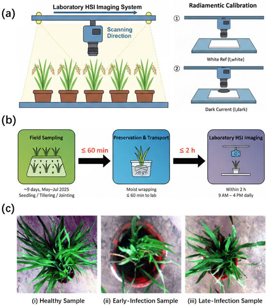
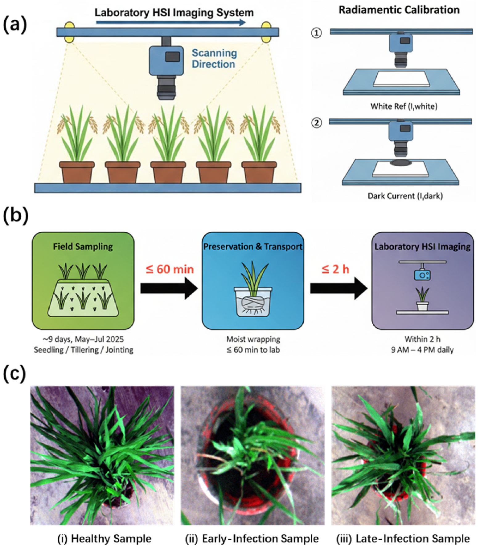
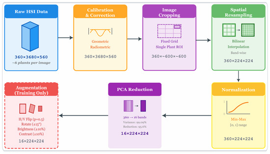
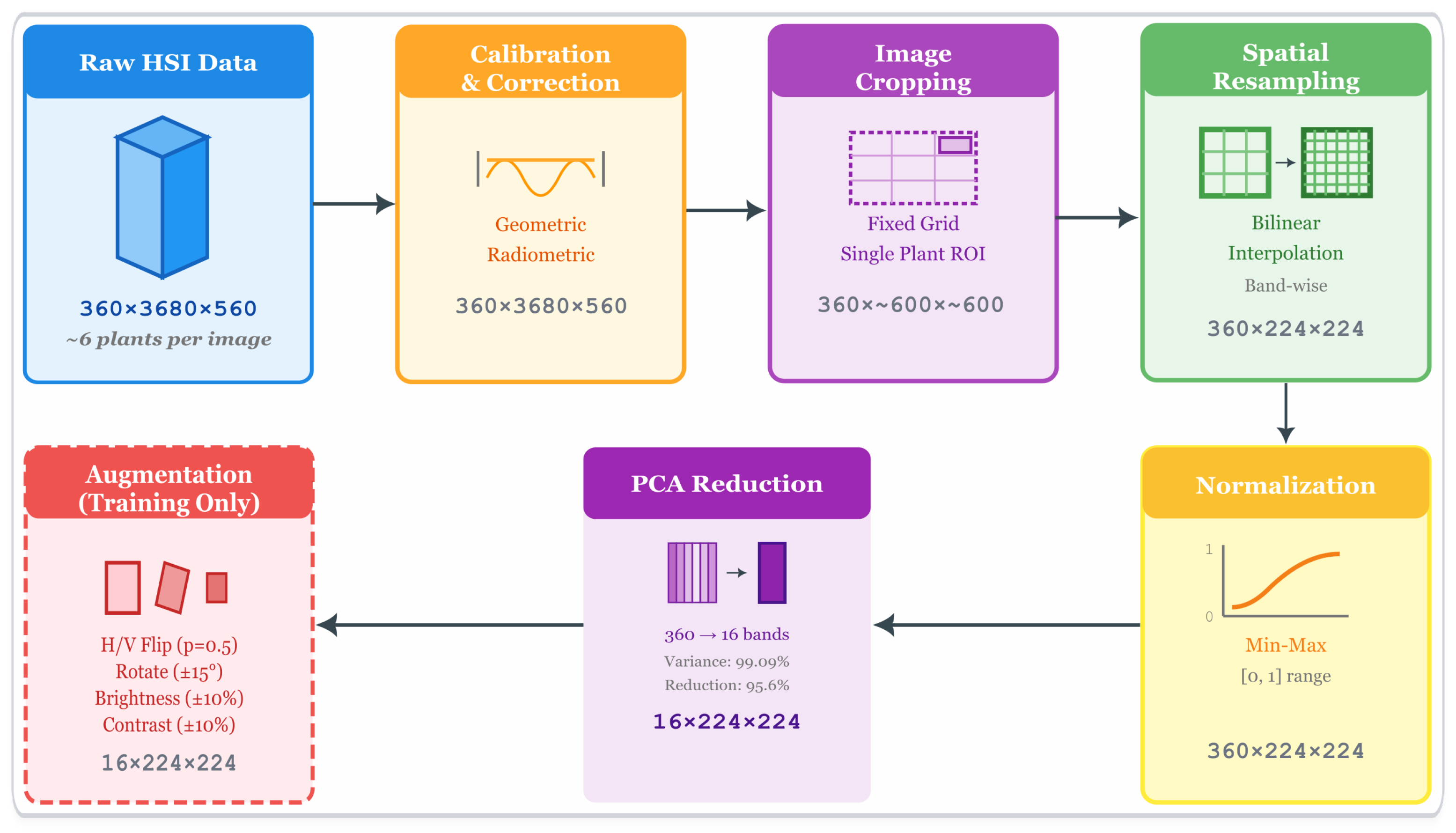
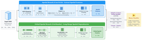
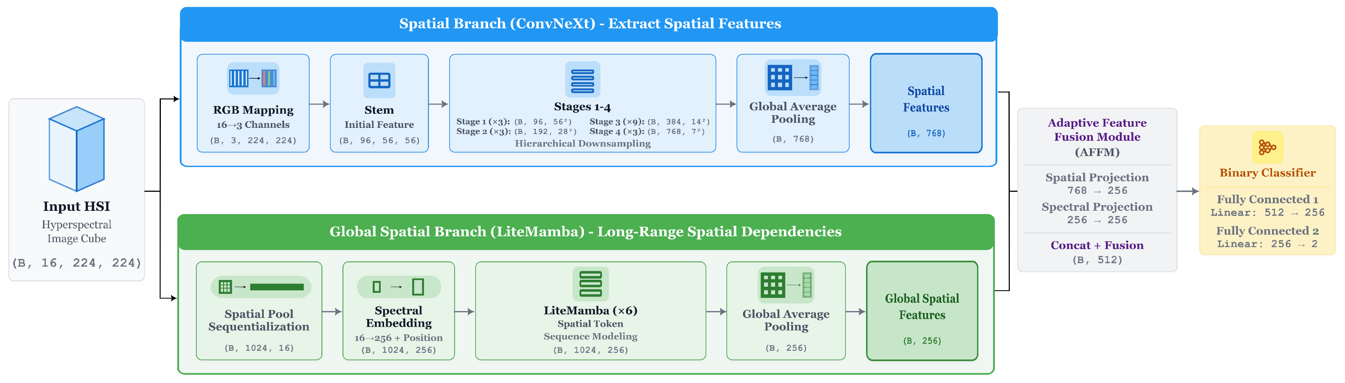
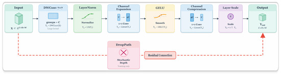
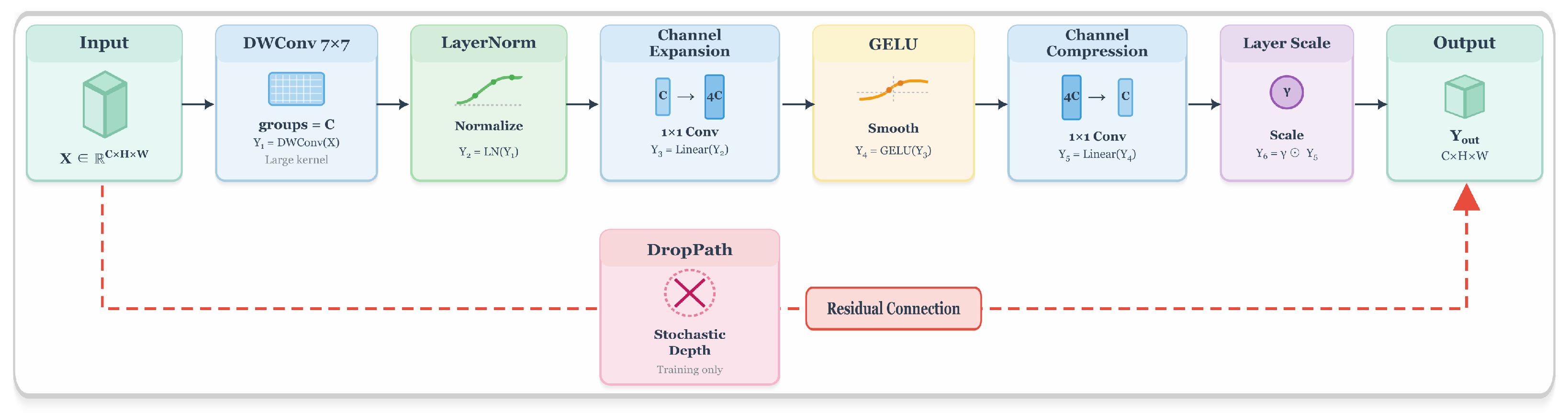
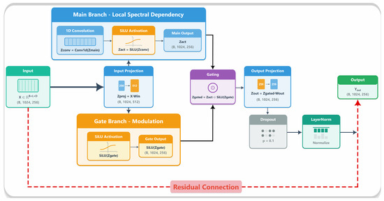
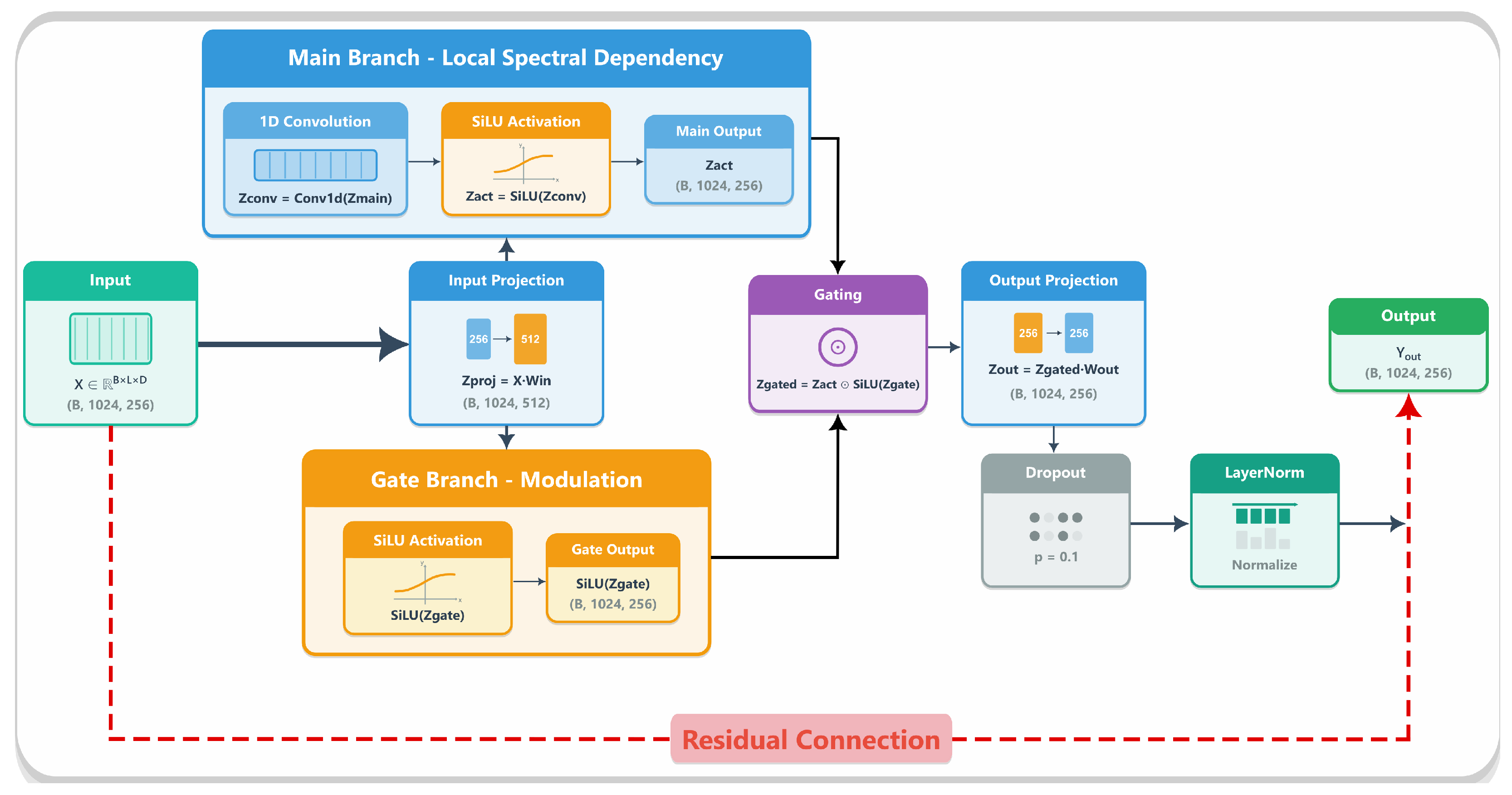
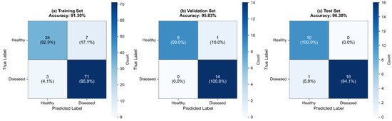
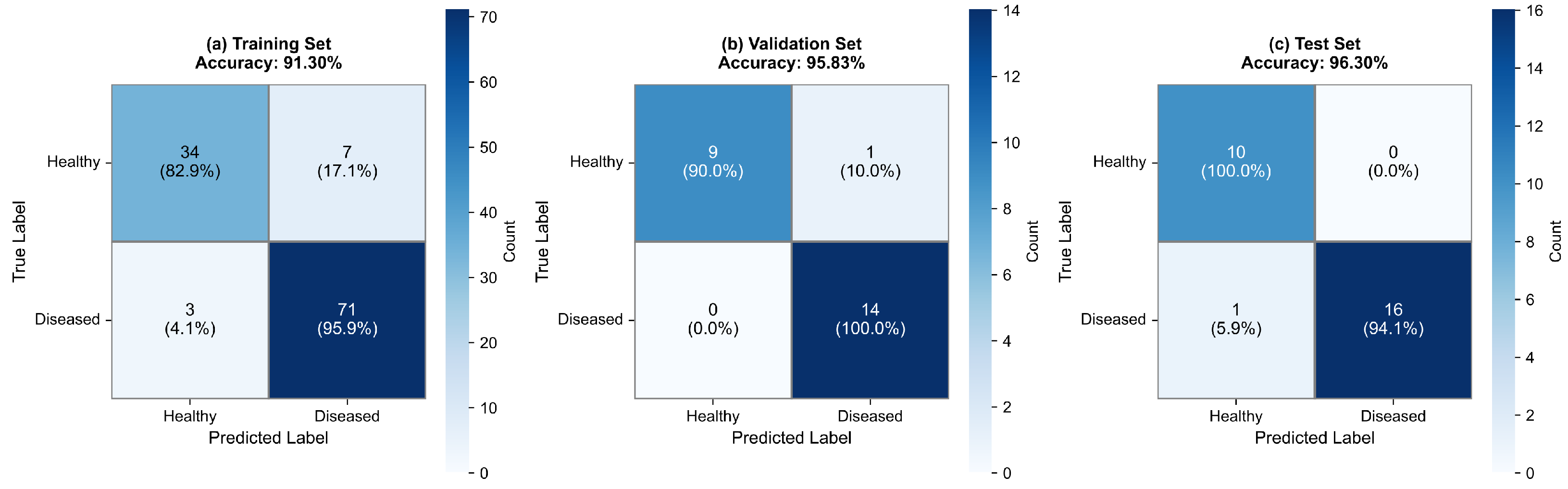
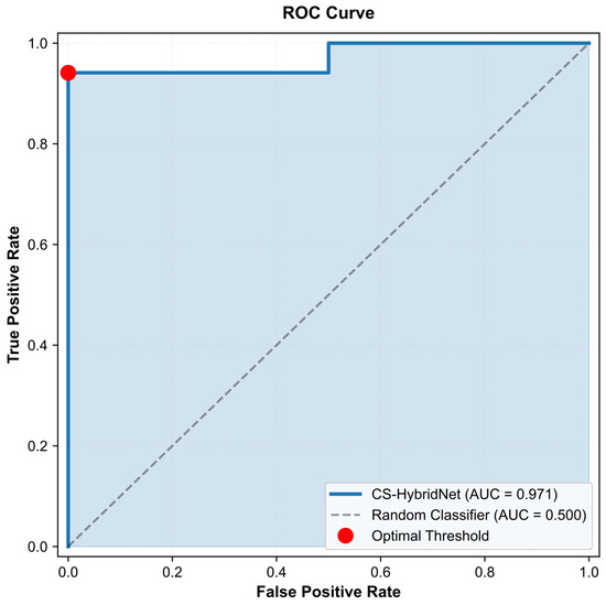
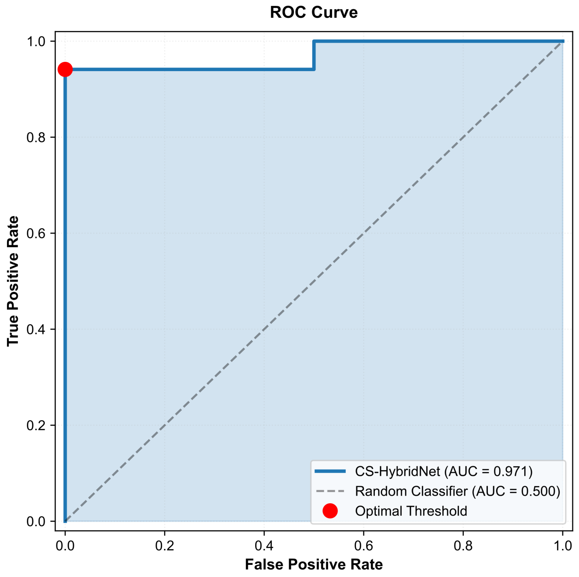
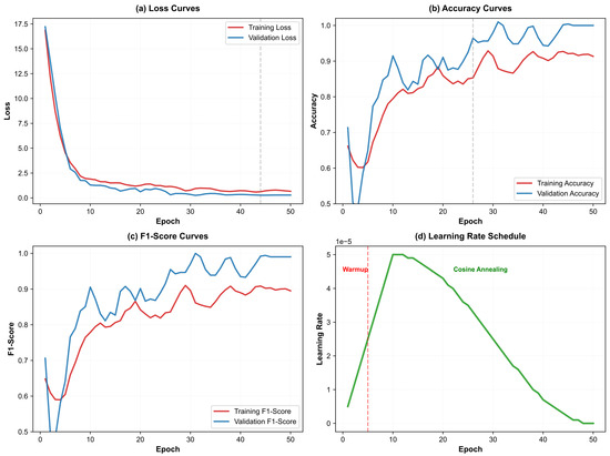
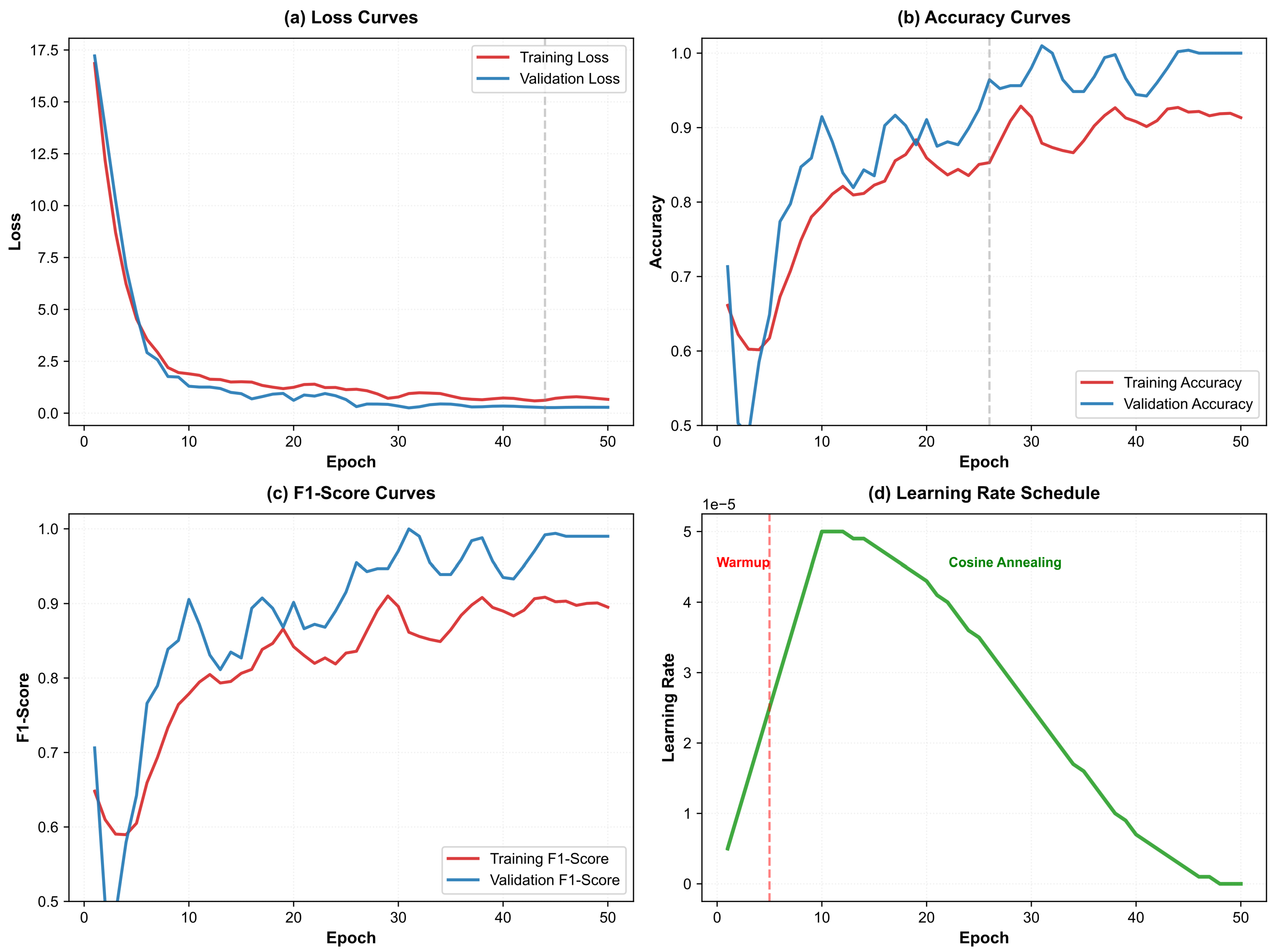
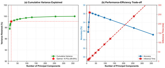
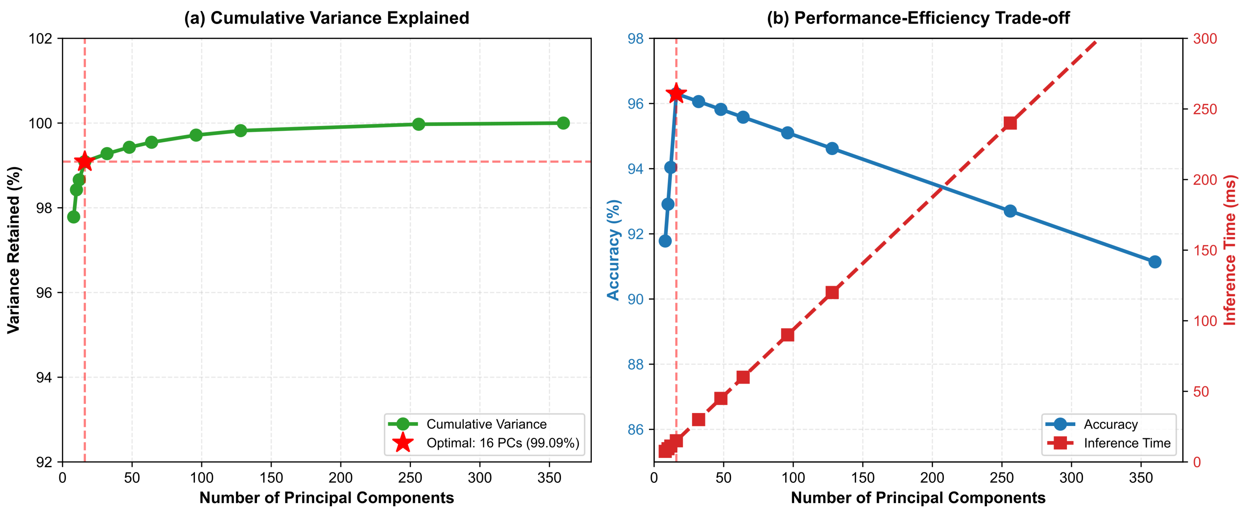
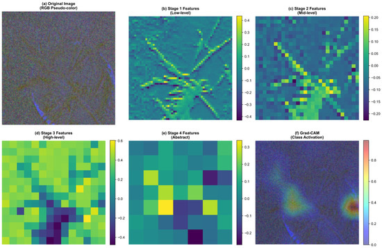
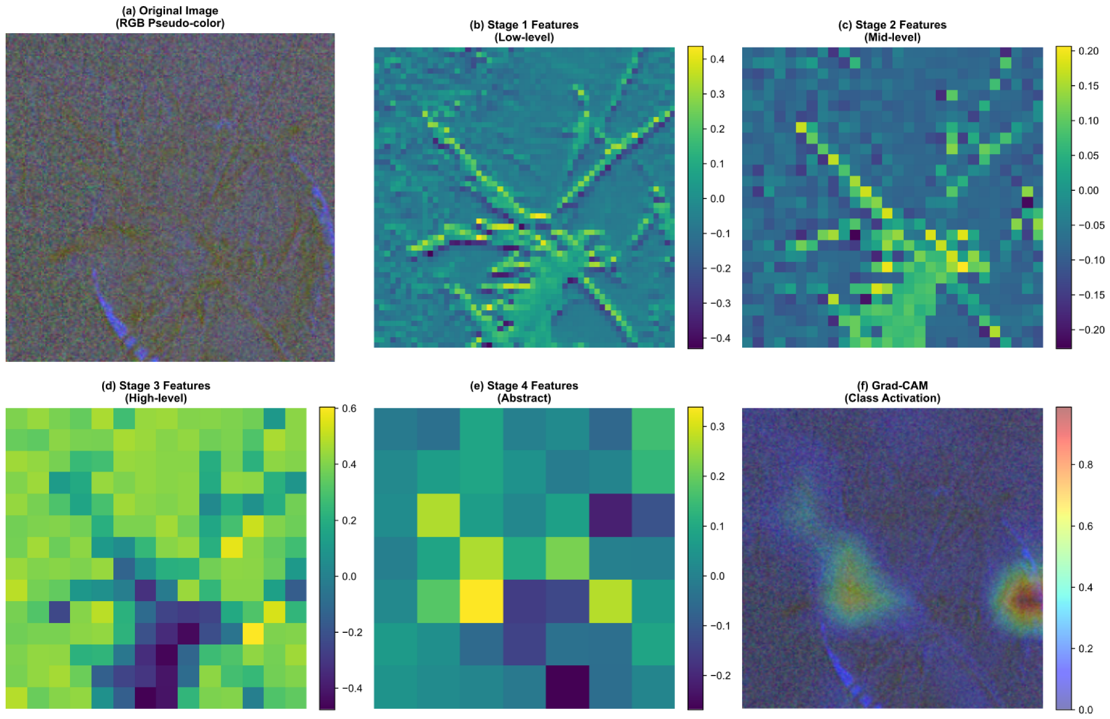
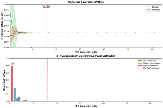
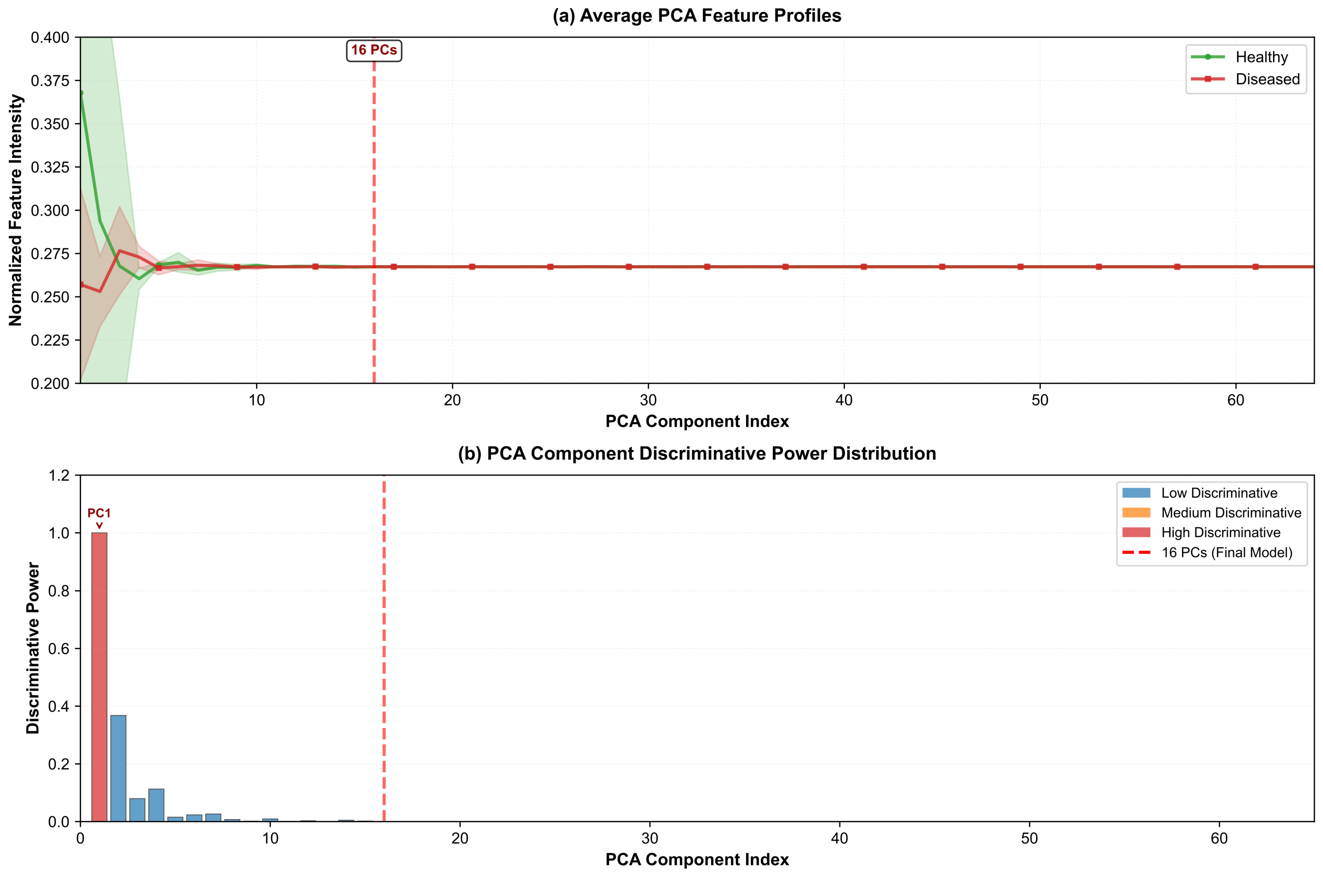
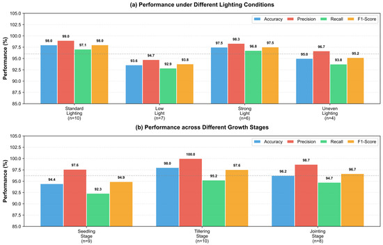
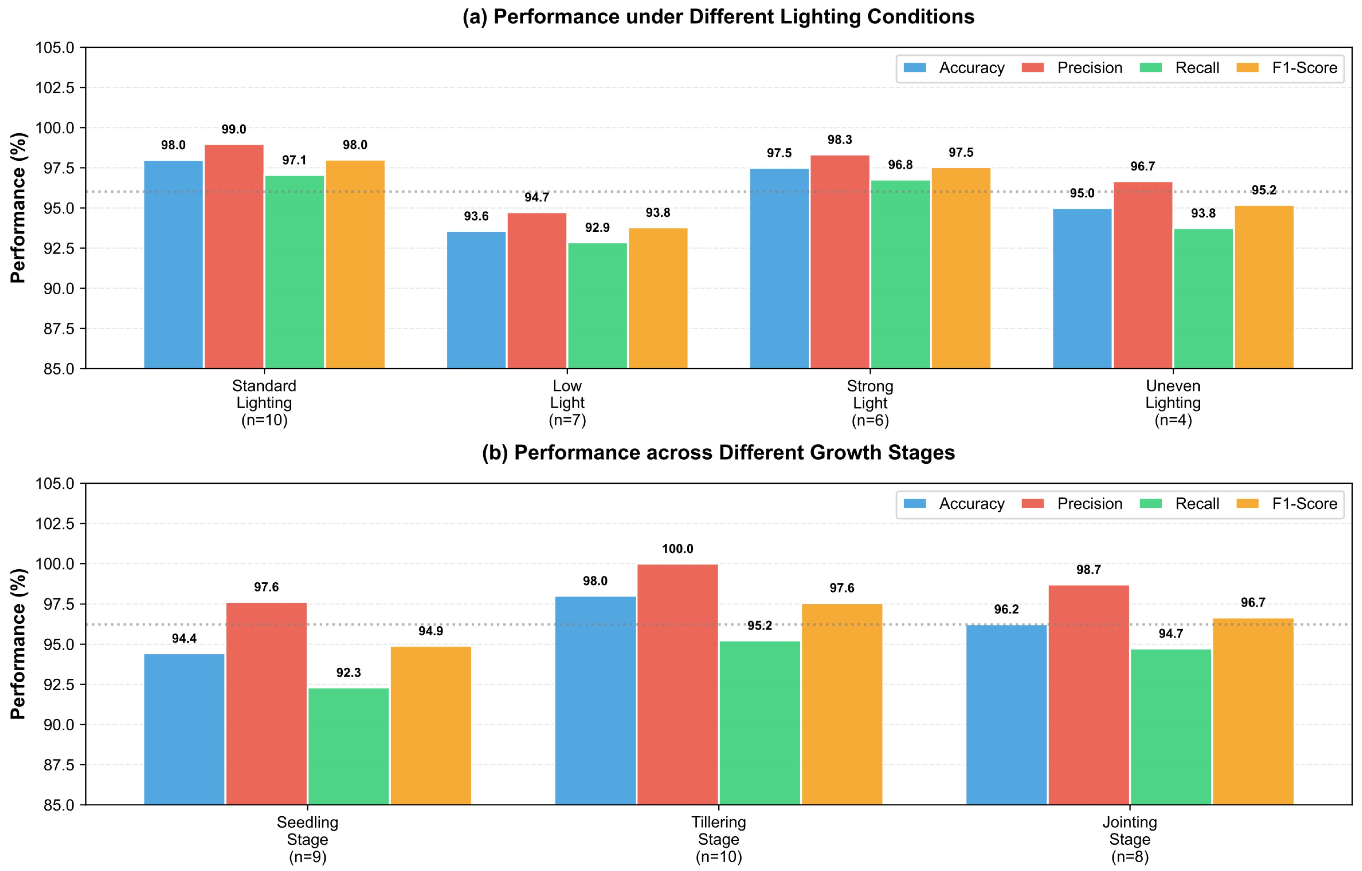

Disclaimer/Publisher’s Note: The statements, opinions and data contained in all publications are solely those of the individual author(s) and contributor(s) and not of MDPI and/or the editor(s). MDPI and/or the editor(s) disclaim responsibility for any injury to people or property resulting from any ideas, methods, instructions or products referred to in the content. |
© 2026 by the authors. Licensee MDPI, Basel, Switzerland. This article is an open access article distributed under the terms and conditions of the Creative Commons Attribution (CC BY) license.