Hyperspectral Estimation of Apple Canopy SPAD Values Based on Optimized Spectral Indices and CEO-LSSVM

Abstract

Leaf chlorophyll content (LCC) is a key physiological parameter affecting plant growth and development. Rapid and non-destructive monitoring of LCC using hyperspectral remote sensing is crucial for promoting precision agriculture. In this study, hyperspectral data of apple canopy leaves at different phenological stages were collected alongside their corresponding SPAD values (representing LCC) to construct a dataset. Two types of spectral features were extracted: (1) optimized spectral index combinations; and (2) feature bands selected using the Successive Projections Algorithm (SPA). Based on these features, three machine learning models—Support Vector Machine (SVM), Least Squares Support Vector Machine (LSSVM), and Chaos Evolution Optimization-enhanced LSSVM (CEO-LSSVM)—were developed to estimate SPAD values. The results indicate that the constructed optimal spectral index combinations exhibit superior sensitivity in SPAD estimation compared to the feature bands selected by SPA. Specifically, during the physiological fruit drop stage, the CEO-LSSVM model based on spectral indices achieved a test set R² of 0.851, surpassing the SPA-based model (R² = 0.813). Regarding model performance, the CEO-LSSVM demonstrated the highest accuracy and robustness across all stages. In the fruit drop period, using optimized spectral indices, it achieved an RMSE of 1.338, significantly outperforming the LSSVM (RMSE = 1.703) and SVM (RMSE = 2.409) models. This superiority was further evident in the fruit enlargement stage, where the CEO-LSSVM model reached a peak test set R² of 0.868 and the lowest RMSE of 1.254. The integrated model combining optimized spectral indices and CEO-LSSVM provides an efficient and high-precision approach for hyperspectral SPAD estimation in apple canopies, effectively addressing the challenges of inversion modeling in arid oasis environments.

1. Introduction

Chlorophyll acts as a fundamental pigment in plant photosynthesis. Its content not only reflects the photosynthetic capacity of plants but is also intricately linked to the senescence process, nitrogen nutritional status, and responses to environmental stress. Consequently, Leaf Chlorophyll Content (LCC) serves as a vital indicator for evaluating plant growth status and nutrient supply [1,2]. Particularly for apples (Malus domestica), a crop of significant economic value, variations in LCC directly influence photosynthetic rates and organic matter accumulation, thereby determining fruit yield and quality [2,3]. The southern region of Xinjiang, characterized as a typical arid oasis agro-ecosystem, features high evaporation, intense solar radiation, and significant diurnal temperature differences. These conditions render fruit trees more sensitive to environmental fluctuations, resulting in complex spatiotemporal LCC dynamics, which impose higher requirements for the real-time capability and adaptability of monitoring techniques [4,5]. The traditional methods for monitoring the chlorophyll content of vegetation, such as spectrophotometry, although highly accurate, are cumbersome and dependent on time-consuming and non-automated processes, making it difficult to meet the timeliness and accuracy requirements of large-scale non-destructive monitoring [6].

Hyperspectral remote sensing, with its advantages of high spectral resolution, continuous narrow bands, and non-destructive detection, has been widely employed for the quantitative retrieval of critical crop biochemical parameters such as LCC. Various spectral preprocessing techniques have been utilized to enhance spectral features and mitigate noise, thereby improving estimation accuracy [7,8,9,10]. For instance, Xiao et al. [11] constructed an inversion model for cotton leaf chlorophyll content by combining seven spectral preprocessing methods with transfer learning. Their results demonstrated that a fine-tuned Convolutional Neural Network (CNN) based on spectra processed by First Derivative (FD) and Standard Normal Variate (SNV) outperformed traditional Partial Least Squares (PLS) and Support Vector Regression (SVR). However, the inherent high correlation between hyperspectral bands often induces severe multicollinearity, leading to model bias, overfitting, or reduced generalization ability [12]. To address this issue, researchers have proposed dimensionality reduction methods based on Vegetation Indices (VIs) and feature wavelength extraction [13]. For example, Cui et al. [14] collected canopy spectral data of winter wheat under different varieties and stress treatments. Considering the spectral response in the red-edge region, they developed combined indices such as RECAI, RECAI/OSAVI, and RECAI/TVI. Comparing these with eight common spectral indices, they found that the novel integrated RECAI/TVI achieved the highest accuracy in predicting LCC, proving that combined indices are more effective than single indices in suppressing soil background noise.

To address the challenges of high-dimensional data, researchers have proposed dimensionality reduction methods based on Vegetation Indices (VIs). For instance, Li et al. [15] constructed 12 vegetation indices based on the visible, red-edge, and near-infrared bands of Sentinel-2 to estimate apple canopy chlorophyll content. Their results indicated that the Support Vector Machine Regression (SVMR) model developed using specific indices (e.g., NDVIgreen + NDVIred + NDVIre) achieved relatively high accuracy and stability. However, standard machine learning models like SVM typically rely on grid search or manual experience for hyperparameter tuning. These traditional optimization strategies are computationally expensive and susceptible to local optima, limiting the model’s ability to fully exploit the information contained in the spectral indices, especially under complex field conditions.

Feature wavelength extraction represents another critical strategy for improving model precision. Ding et al. [16] employed the Successive Projections Algorithm (SPA) to extract feature wavelengths from preprocessed Raman spectra of cucumbers at different storage stages and constructed a SPA-Extreme Learning Machine (SPA-ELM) model. The results indicated that this method significantly enhanced the inversion accuracy for both chlorophyll content and hardness. Furthermore, Gao et al. [17] utilized near-ground multispectral data for the non-destructive estimation of maize chlorophyll content. By adopting the Iterative Retained Information Variable-Successive Projections Algorithm (IRIV-SPA) to select feature bands, they built a 1D-CNN-GRU model. Their experiments showed that the deep learning model based on feature bands not only reduced data dimensionality but also yielded prediction accuracies significantly superior to full-band models. Despite the progress achieved using single dimensionality reduction strategies (utilizing either indices or feature selection alone), few studies have explored the synergistic integration of multiple feature selection methods. Moreover, the generalizability of existing models across different crop phenological stages remains to be improved.

Furthermore, as perennial fruit trees, apples exhibit distinct physiological activities and nutrient allocation patterns across different phenological stages, which directly impact canopy structure and hyperspectral responses [1,18]. Therefore, the selection of phenological stages is a critical factor for enhancing the accuracy and robustness of hyperspectral LCC inversion [19]. This study selected the physiological fruit drop stage (approximately 5–6 weeks after flowering) and the fruit expansion stage (July–September) as key monitoring windows. The physiological fruit drop stage is characterized by intense nutrient competition among new shoots, young fruits, and roots, resulting in significant LCC gradients that facilitate the sensitive capture of subtle changes in leaf microstructure and pigments by spectral signals. In contrast, during the fruit expansion stage, LCC tends to stabilize and the canopy structure matures, significantly reducing spectral noise, which aids in constructing quantitative models with higher generalization capabilities [20]. Combining these two stages—characterized by high sensitivity and high stability, respectively—creates complementary advantages in the temporal dimension, effectively capturing dynamic LCC changes and providing a reliable data foundation for establishing high-precision and robust inversion models.

In summary, this study uses the apple orchard at Hongqi Slope Farm in Wensu County, Aksu Prefecture, Xinjiang Uygur Autonomous Region, as the research area, with the “Fuji” variety apple tree canopy leaves as the study object. The spectral response differences between the physiological fruit drop and fruit expansion stages are compared, and the variations in leaf reflectance under different spectral preprocessing combinations are explored. To improve the hyperspectral quantitative inversion ability of apple canopy chlorophyll content, this study constructs various spectral index combinations, applies the successive projection algorithm (SPA) to extract the feature bands most sensitive to chlorophyll, and introduces a chaotic evolutionary algorithm to optimize the least squares support vector machine (CEO-LSSVM). The precision of different models is compared to build a high-precision and robust inversion model for apple leaf chlorophyll content, aiming to provide theoretical support for rapid monitoring in regional orchards.

2. Materials and Methods

2.1. Study Area and Plant Materials

This study was conducted at the Hongqipo Farm in Aksu Prefecture, Xinjiang Uygur Autonomous Region (40°38′–40°45′ N, 80°20′–80°32′ E). Situated at the convergence of the southern foothills of the Tianshan Mountains and the northern edge of the Tarim Basin, the region features a typical warm temperate continental arid oasis climate. The area is characterized by abundant sunshine, significant diurnal temperature variations, and rich thermal resources, providing optimal natural conditions for fruit cultivation [21]. The predominant soil textures in the region include saline-alkaline soil, light loam, and sandy loam, with pH values typically ranging from 7.5 to 8.2. The soil exhibits good permeability but relatively low organic matter content, which is representative of the edaphic characteristics of oases in southern Xinjiang [5]. The orchard of Hongqi Po Farm adheres to standardized management norms. The row and plant spacing of apple trees in the park is 5 m × 6 m, which is an ideal place for hyperspectral remote sensing and physiological monitoring. The primary apple cultivar in the study area is ‘Fuji’. Based on actual growth conditions, 100 apple trees (aged 8–12 years) exhibiting consistent vigor and free from pests and diseases were selected and tagged as experimental subjects. Experiments were conducted during two key phenological stages: the physiological fruit drop stage (June) and the fruit expansion stage (July), to explore the relationship between canopy hyperspectral data and the physiological status of the trees.

2.2. Data Collection

2.2.1. Hyperspectral Data Acquisition

Hyperspectral data of apple canopy leaves were acquired using an ASD FieldSpec HandHeld 2 portable spectrometer (Analytical Spectral Devices Inc., Boulder, CO, USA). The instrument has a spectral range of 325–1075 nm with a sampling interval of 1.4 nm and a spectral resolution of approximately 3 nm, enabling the effective capture of subtle spectral variations associated with plant biochemical properties. Spectral measurements were conducted strictly during two specific periods: 16–18 June 2025 (physiological fruit drop stage) and 17–20 July 2025 (fruit expansion stage). To ensure the representativeness and physiological consistency of the samples, fully expanded mature functional leaves (typically the 3rd to 5th leaf from the shoot tip) were selected from the outer, sun-exposed periphery of the canopy. Data collection was strictly restricted to the time window of 10:00 AM to 2:00 PM local time under clear, cloudless conditions to minimize the impact of varying solar illumination and atmospheric changes on spectral reflectance. To ensure radiometric accuracy, the instrument was calibrated using a standard white reference panel (Spectralon) every 15 min. The reflectance of the calibrated panel was verified to be 1 across the entire spectral range. During measurements, leaf samples were placed against a low-reflectance black background. The fiber optic probe was positioned vertically (nadir view) at a fixed distance of 15–20 cm above the leaf surface, with a field of view (FOV) of 25°. For each leaf sample, 20 spectral scans were averaged to produce a single representative spectral curve. All data were recorded using ViewSpec Pro 6.2.0 software (ASD Inc., Boulder, CO, USA). Savitzky–Golay (SG) smoothing was subsequently applied to the hyperspectral data to mitigate random noise, particularly at the spectral edges, ensuring the reliability of feature extraction and model construction.

2.2.2. Canopy Leaf SPAD Value Measurement

Leaf Chlorophyll Content (LCC) was represented by SPAD values measured using a SPAD-502 Plus portable chlorophyll meter (Konica Minolta, Tokyo, Japan), concurrently with spectral data acquisition. To account for the heterogeneous distribution of chlorophyll within the leaf tissue, measurements were taken at five distinct positions along the leaf margins, strictly avoiding major veins and petioles. The average of these five readings was recorded as the final SPAD value for each leaf. In this study, leaf samples were collected from 100 tagged apple trees across two phenological stages (June and July), resulting in a cumulative dataset of 420 samples (N = 420).

2.3. Data Preprocessing

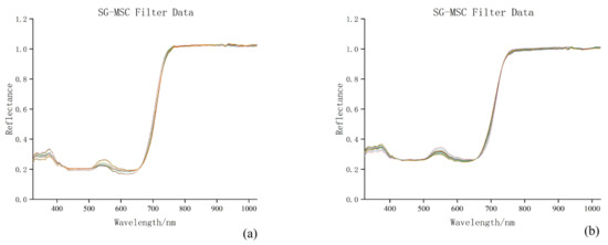
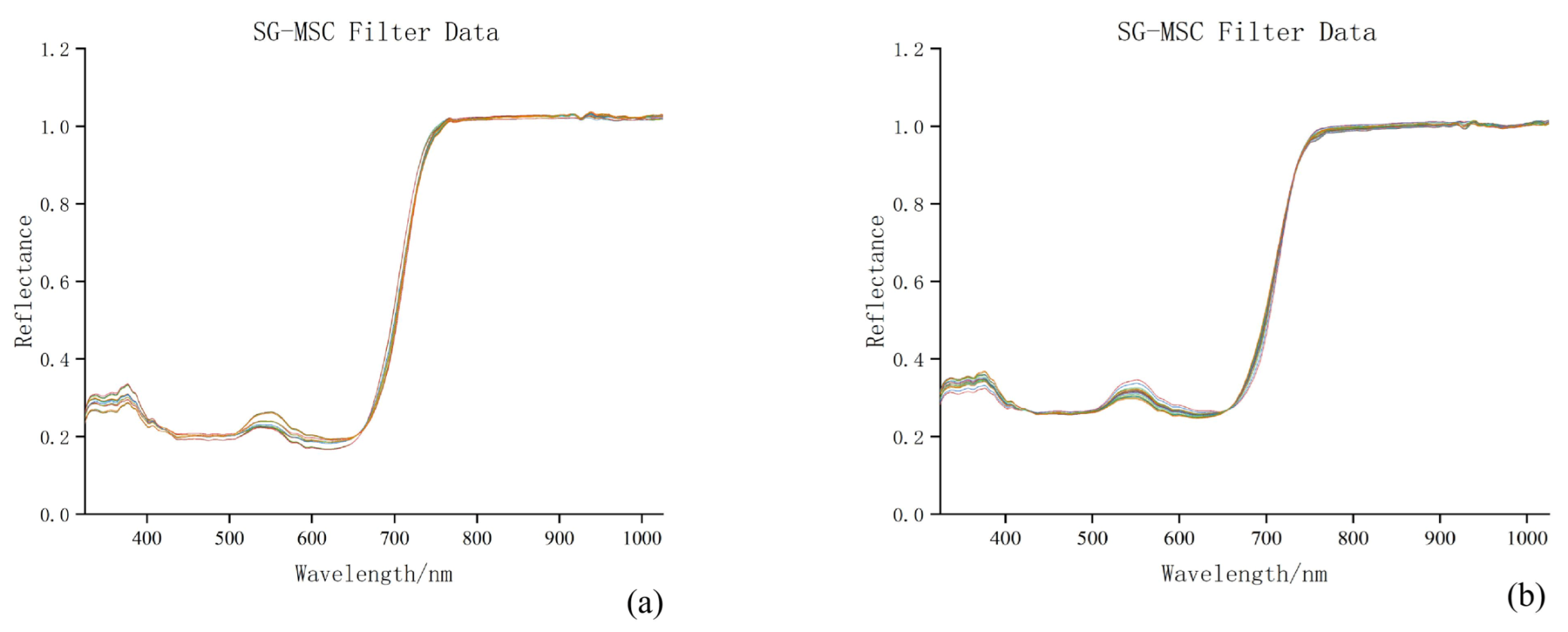
During the collection of hyperspectral data from apple leaves, factors such as the condition of the samples, environmental changes, and instrument stability could cause baseline drift, random noise, and scattering in the spectral data, which may affect the accuracy of model construction. Therefore, preprocessing was performed on the raw spectra to reduce interference and improve the signal-to-noise ratio (SNR). This study used a combination of Savitzky–Golay (SG) smoothing and Multivariate Scatter Correction (MSC) for preprocessing. SG smoothing was primarily used to eliminate random noise and filter high-frequency signals, while MSC was used to correct for baseline drift and light scattering variations. The results are shown in Figure 1.

Figure 1. MapResults of SG-MSC preprocessing. Different colored lines represent the spectral reflectance curves of individual leaf samples (a) Preprocessed spectral data for June; (b) Preprocessed spectral data for July.

2.4. Spectral Feature Extraction

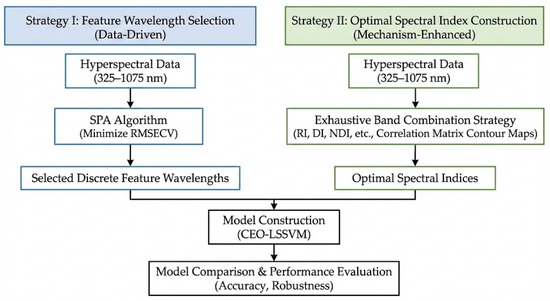
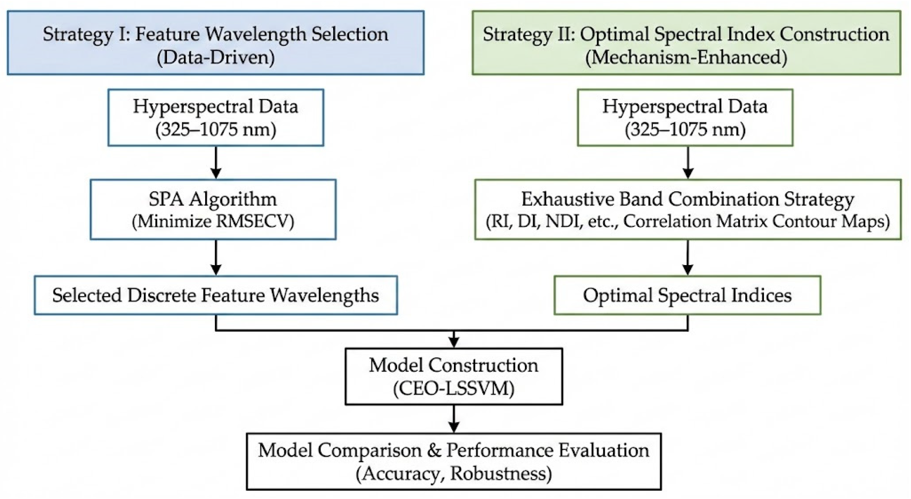
To investigate the impact of different dimensionality reduction strategies on the accuracy of chlorophyll content (LCC) inversion in apple leaves, this study compares two independent spectral feature extraction approaches: one based on feature wavelength selection using data mining algorithms, and the other based on the construction of optimal spectral indices based on spectral response mechanisms. By comparing the features extracted using these two methods, the study analyzes their differences in eliminating redundancy, suppressing background noise, and improving model interpretability, in order to determine the optimal input features for modeling. The technical route is shown in Figure 2.

Figure 2. Technical roadmap.

2.4.1. Feature Wavelength Selection Method

Hyperspectral data are characterized by high dimensionality and strong inter-band correlations. Directly inputting such high-dimensional data into regression models often leads to multicollinearity and overfitting, thereby reducing the model’s generalization ability. Therefore, the Successive Projections Algorithm (SPA) was employed to perform dimensionality reduction on the spectral data in the 325–1075 nm range.

SPA is a forward variable selection algorithm designed to select a subset of bands with minimal redundancy and collinearity through projection operations. The algorithm starts with an initial band, and in each iteration, introduces a new candidate band that has the maximum projection vector magnitude in the orthogonal subspace, thus maximizing the new information content [22,23]. In this study, the original spectral reflectance matrix served as the input variable, while the measured SPAD values served as the output variable. The optimal number of bands was determined based on the minimum root mean square error of cross-validation (RMSECV) obtained from multiple linear regression (MLR). Through this process, a subset of spectral bands most sensitive to apple leaf chlorophyll content was selected. These selected feature bands (primarily distributed in the visible absorption valley, red edge, and near-infrared plateau regions) were then used as input variables for the subsequent machine learning models, effectively reducing model complexity while retaining key spectral response features.

2.4.2. Optimal Spectral Index Construction Method

Unlike using a single band directly, spectral indices enhance sensitivity to weak spectral signals and effectively suppress external noise interferences such as soil background and uneven lighting through mathematical operations between bands (such as ratios, differences, etc.). Previous studies have shown that various spectral indices demonstrate good indicative capabilities for monitoring vegetation physiological structure and biochemical characteristics. The Ratio Index (RI) and Triangular Vegetation Index (TVI) show high sensitivity in assessing chlorophyll content, but they are prone to saturation in response when vegetation is dense. The Modified Simple Ratio (mSR) and Modified Normalized Difference Index (mNDI) can effectively reduce specular reflection interference in the red-edge region, offering better recognition of changes in leaf structure. The Difference Index (DI), Normalized Difference Vegetation Index (NDVI), and Soil-Adjusted Vegetation Index (SAVI) are advantageous in reducing soil background effects and radiation noise, showing more stable performance at the canopy scale. Therefore, this study selects seven classic vegetation indices as shown in Table 1, and constructs them using an exhaustive band combination strategy. The formulas for these indices are detailed in Table 1, where $R_i$ and $R_j$ represent the preprocessed spectral reflectance values at any wavelength positions.

Table 1. Spectral Index Names and Formulas.

Spectral Index Name	Spectral Index Calculation Formula	Reference
Ratio Vegetation Index/RI	$R_i/R_j$	[24]
Difference Vegetation Index/DVI	$R_i-R_j$	[25]
Normalized Difference Vegetation Index/NDVI	$(R_i-R_j)/(R_i+R_j)$	[26]
Soil Adjusted Vegetation Index/SAVI	$(1+0.16){\displaystyle \frac{R_i-R_j}{R_i+R_{j}0.16}}$	[27]
Reciprocal Difference Vegetation Index/RDVI	$1/R_i-1/R_j$	[28]
Triangular Vegetation Index/TVI	$0.5\times (120\times (R_i-R_{550})-200\times (R_j-R_{550}))$	[29]
Modified Simple Ratio/mSR	$(R_i/R_j-1)/\sqrt{(R_i/R_j+1)}$	[9]

2.5. Model Construction Method

In this study, spectral index combinations and the SPA-selected feature bands are used as input variables, with the SPAD value of the canopy leaves serving as the output variable. To explore the applicability of different regression algorithms in the inversion of chlorophyll content in apple canopies, three nonlinear regression models are constructed: Support Vector Regression (SVR), Least Squares Support Vector Machine (LSSVM), and the LSSVM optimized by a Chaos Evolutionary Algorithm (CEO-LSSVM). The construction and validation of all models are implemented using the Matlab 2024 (MathWorks, Natick, MA, USA) platform.

2.5.1. SVM

Support Vector Machine (SVM) is based on the structural risk minimization principle and demonstrates excellent generalization ability in solving small-sample, high-dimensional, and non-linear regression problems [30,31]. In this study, the $\epsilon -\mathrm{SVR}$ algorithm was adopted to construct the SPAD inversion model. Assume a training sample set, where $x_i\in R^d$ represents the input spectral feature vector, $y_i\in R$ is the corresponding SPAD value, and $N$ is the number of samples. The goal of SVR is to find a regression function $f(x)={\omega }^T\phi (x)+b$, such that the difference between the predicted value and the actual value does not exceed the threshold $\epsilon$. Here, $\phi (x)$ denotes the non-linear mapping function that maps the input space to a high-dimensional feature space, $\omega$ is the weight vector, and $b$ is the bias term. By introducing slack variables ${\xi }_i$ and ${\xi }_i^{*}$ L, the optimization problem of SVR can be described as:

$$\underset{\omega ,b,\xi ,{\xi }^{*}}{\min }{\displaystyle \frac{1}{2}}{‖\omega ‖}^2+C{\displaystyle \sum _{i=1}^N({\xi }_i+{\xi }_i^{*})}$$

(1)

$$s.t.\left\{\begin{array}{c}{y}_i-({\omega }^T\phi (x_i)+b)\le \epsilon +{\xi }_i\\ ({\omega }^T\phi (x_i)+b)-y_i\le \epsilon +{\xi }_i^{*}\\ {\xi }_i,{\xi }_i^{*}\ge 0,i=1,\dots ,N\end{array}\right.$$

(2)

$$f(x)={\displaystyle \sum _{i=1}^N({\alpha }_i-{\alpha }_i^{*})K(x_i,x)+b}$$

(3)

2.5.2. LSSVM

The Least Squares Support Vector Machine (LSSVM) is an improved variant of the standard SVM. Its core principle involves replacing the inequality constraints found in standard SVM with equality constraints and adopting a squared error loss function. This transformation converts the optimization problem, which originally required Quadratic Programming (QP), into the solution of a system of linear equations. This characteristic not only significantly reduces computational complexity but also renders LSSVM particularly suitable for typical hyperspectral data analysis tasks characterized by high dimensionality and small sample sizes [32,33]. The form of its regression function is expressed as:

$$f(x)={\omega }^T\varphi (x)+b$$

(4)

The optimization problem of LSSVM is formulated as follows:

$$\underset{\omega ,b,e_i}{{\displaystyle \min }}J(\omega ,e_i)={\displaystyle \frac{1}{2}}{‖\omega ‖}^2+{\displaystyle \frac{\gamma }{2}}{\displaystyle \sum _{i=1}^m{e}_i^2}$$

(5)

$$s.t.y_i={\omega }^T\varphi (x_i)+b+e_i$$

(6)

where $e_i$ represents the error term and $\gamma$ is the penalty factor. By applying the Lagrange multiplier method, the following system of linear equations is obtained:

$$\left[\begin{array}{cc}0& 1^T\\ 1& \Omega +{\gamma }^{-1}I\end{array}\right]\left[\begin{array}{c}b\\ \alpha \end{array}\right]=\left[\begin{array}{c}0\\ y\end{array}\right]$$

(7)

where ${\Omega }_{i,j}=K(x_i,x_j)$

Similarly to the SVM model, the RBF kernel function was selected in this study. Additionally, the hyperparameter ranges were kept consistent with those of the SVM to ensure fairness and comparability.

2.5.3. CEO-LSSVM

Although LSSVM boasts higher computational efficiency compared to traditional SVM, its performance remains heavily dependent on the selection of the penalty factor $\gamma$ and kernel width $\sigma$. Traditional search strategies, such as grid search, incur high computational overhead and are prone to becoming trapped in local optima. To enhance model accuracy and parameter optimization efficiency, this study introduces the Chaos Evolution Optimization (CEO) algorithm to optimize the hyperparameters of the LSSVM.

CEO is a population-based intelligent optimization algorithm. Its core principle lies in utilizing chaotic sequences—characterized by ergodicity and pseudo-randomness—within the parameter space to generate diverse search trajectories. By employing mutation–crossover–selection mechanisms to accelerate local convergence, the algorithm effectively improves convergence efficiency while maintaining global search capability [34].

$$\left\{\begin{array}{c}{x}_{t+1}=k{e}^{-\pi y_t}{x}_t\\ y_{t+1}=y_t+x_t\end{array}\right.$$

(8)

where $k$ represents the scaling factor. This mapping generates well-distributed chaotic sequences within the interval [−1, 1], which are utilized for generating search directions.

In this study, the CEO algorithm is employed to search for the hyperparameter vector of the LSSVM.

$$\theta =[\gamma ,\sigma ]$$

(9)

Multiple search directions are generated using chaotic mapping to enhance population diversity; candidate solutions are constructed via a binomial crossover mechanism to strengthen local search capability; and superior solutions are selected based on the objective function (5-fold cross-validation RMSE). Meanwhile, two types of mutation results—based on the best individual and ordinary individuals—are updated simultaneously to accelerate convergence and prevent premature convergence.

In the experiments, the parameters for CEO-LSSVM were set as follows: a population size of 10, a chaotic sample count of 6, and a maximum of 10 iterations. The iteration process was executed in an independent parallel manner. This method significantly reduces computational costs while ensuring global search capability, rendering it suitable for the repetitive validation processes required for high-dimensional spectral data.

2.5.4. Data Partitioning

The cumulative dataset for this study consisted of 420 leaf samples, comprising 210 samples collected during the physiological fruit drop stage and 210 samples during the fruit enlargement stage. To ensure that the calibration set comprehensively represented the spectral variability of the entire dataset, the Kennard-Stone (KS) algorithm [35] was employed to partition the samples, rather than a simple random split. The dataset was divided into a calibration set and a prediction set at a ratio of 3:1. Consequently, 315 samples were allocated for model calibration to ensure robust learning of the spectral features, while the remaining 105 samples were used for independent validation. This partition strategy ensures that the model is trained on a representative subset while being evaluated on a strictly independent dataset.

2.6. Model Evaluation

To thoroughly validate the performance of the model, the coefficient of determination $R^2$ and the root mean square error (RMSE) are selected to comprehensively evaluate the accuracy of the apple leaf SPAD value inversion model. The closer $R^2$ is to 1 and the smaller the RMSE, the higher the model accuracy and the better the inversion estimation ability [36]. The calculation formulas are given in Equations (10) and (11).

$$R^2={\displaystyle \frac{{\displaystyle \sum _{i=1}^n{(x_i-\overline{x})}^2}{(y_i-\overline{y})}^2}{{\displaystyle \sum _{i=1}^n{(x_i-\overline{x})}^2}{\displaystyle \sum _{i=1}^n{(y_i-\overline{y})}^2}}}$$

(10)

$$RMSE=\sqrt{{\displaystyle \frac{{\displaystyle \sum _{i=1}^n{(x_i-y_i)}^2}}{n}}}$$

(11)

where $x_i$ is the measured value of the apple leaf SPAD, $\overline{x}$ is the mean of the measured SPAD values; $y_i$ is the predicted value of SPAD from the estimation model, and $\overline{y}$ is the mean of the predicted SPAD values, and $n$ is the number of samples.

3. Results

3.1. Selection and Analysis of Sensitive Feature Bands

3.1.1. Feature Band Extraction Based on SPA

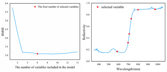
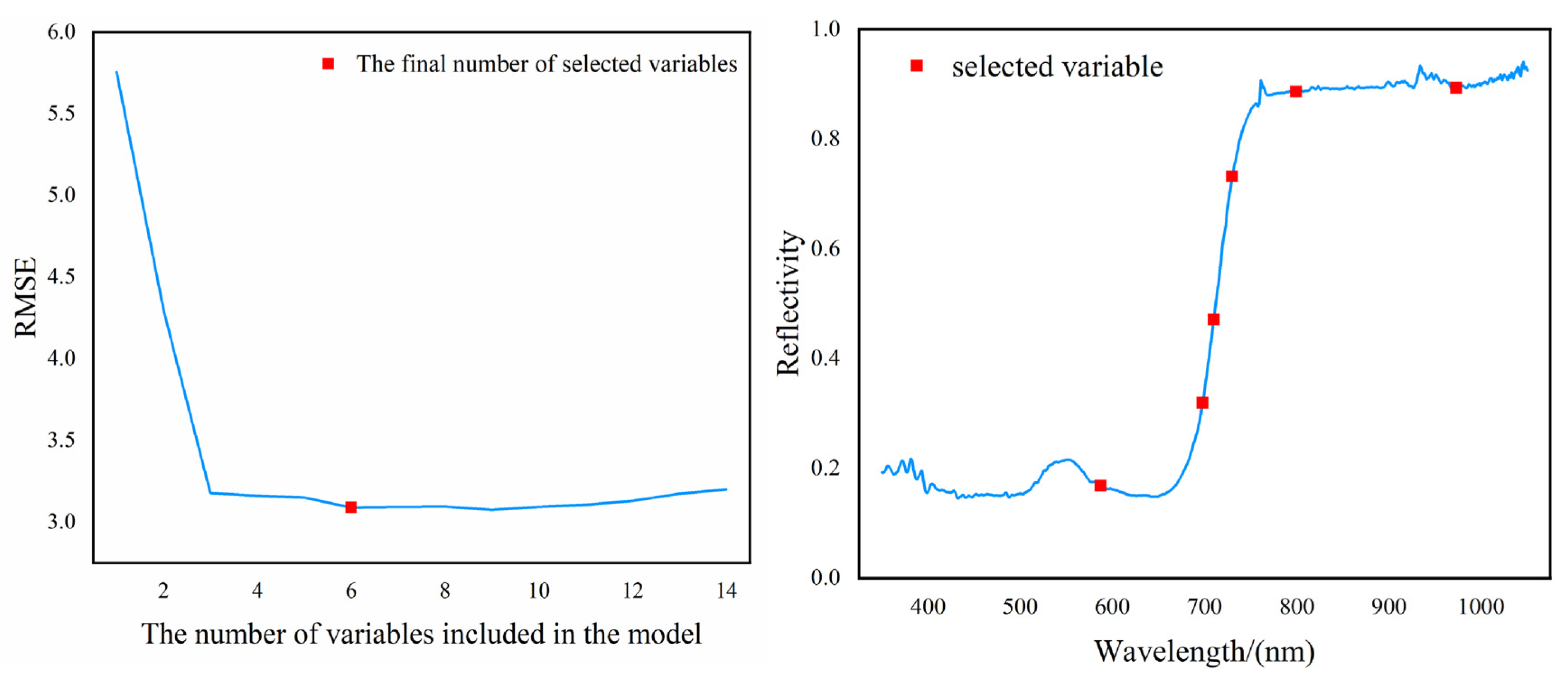
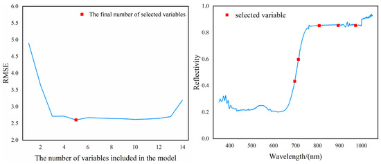
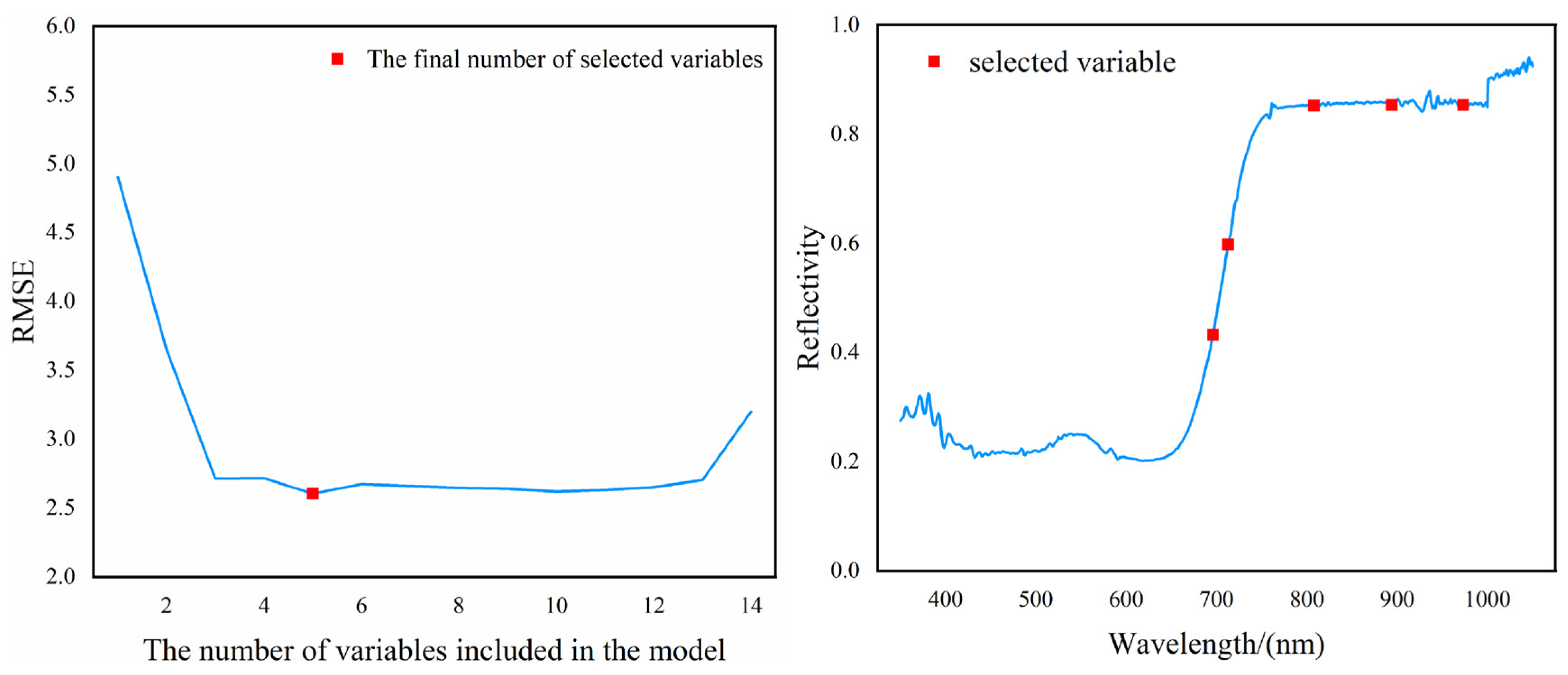
Figure 3 and Figure 4 illustrate the relationship between the number of selected feature variables and the model’s root mean square error (RMSE). Initially, as the number of variables increases from 1 to 6, the RMSE exhibits a sharp decline (dropping from approximately 6.0 to 3.5), indicating a rapid improvement in model accuracy. However, when the number of variables exceeds this range (typically 5–10), the decline in RMSE significantly decelerates and the curve tends to plateau. This suggests that adding further variables contributes marginally to model accuracy but increases the risk of multicollinearity and overfitting, thereby compromising generalization ability.

Figure 3. June Feature Extraction Map.

Figure 4. July Feature Extraction Map.

Consequently, based on the RMSE inflection point criterion, the optimal numbers of feature bands were determined to be 6 and 5 for the two phenological periods, respectively. This selection strategy achieved a dimensionality reduction rate exceeding 99%, significantly simplifying the model structure while retaining critical spectral information.

As shown in Figure 3, during the physiological fruit drop period, the SPA algorithm selected six feature bands: 587 nm, 698 nm, 710 nm, 730 nm, 799 nm, and 973 nm. These bands are distributed across the visible green region, the red-edge, and the near-infrared plateau, including a water-sensitive band at 973 nm.

Similarly, as shown in Figure 4, the SPA algorithm identified five characteristic wavelengths during the fruit enlargement period: 529 nm, 696 nm, 713 nm, 808 nm, and 894 nm. These selected bands are distributed across the visible green peak, the red-edge region, and the near-infrared plateau. Notably, compared to the physiological fruit drop stage, the specific water-sensitive bands (e.g., around 973 nm) were not selected in this period. The detailed physical interpretation of these bands and their physiological implications are discussed in Section 4.1.

3.1.2. Optimal Spectral Index Construction Based on Correlation Matrix Method

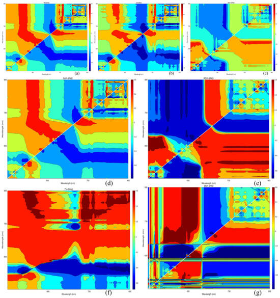
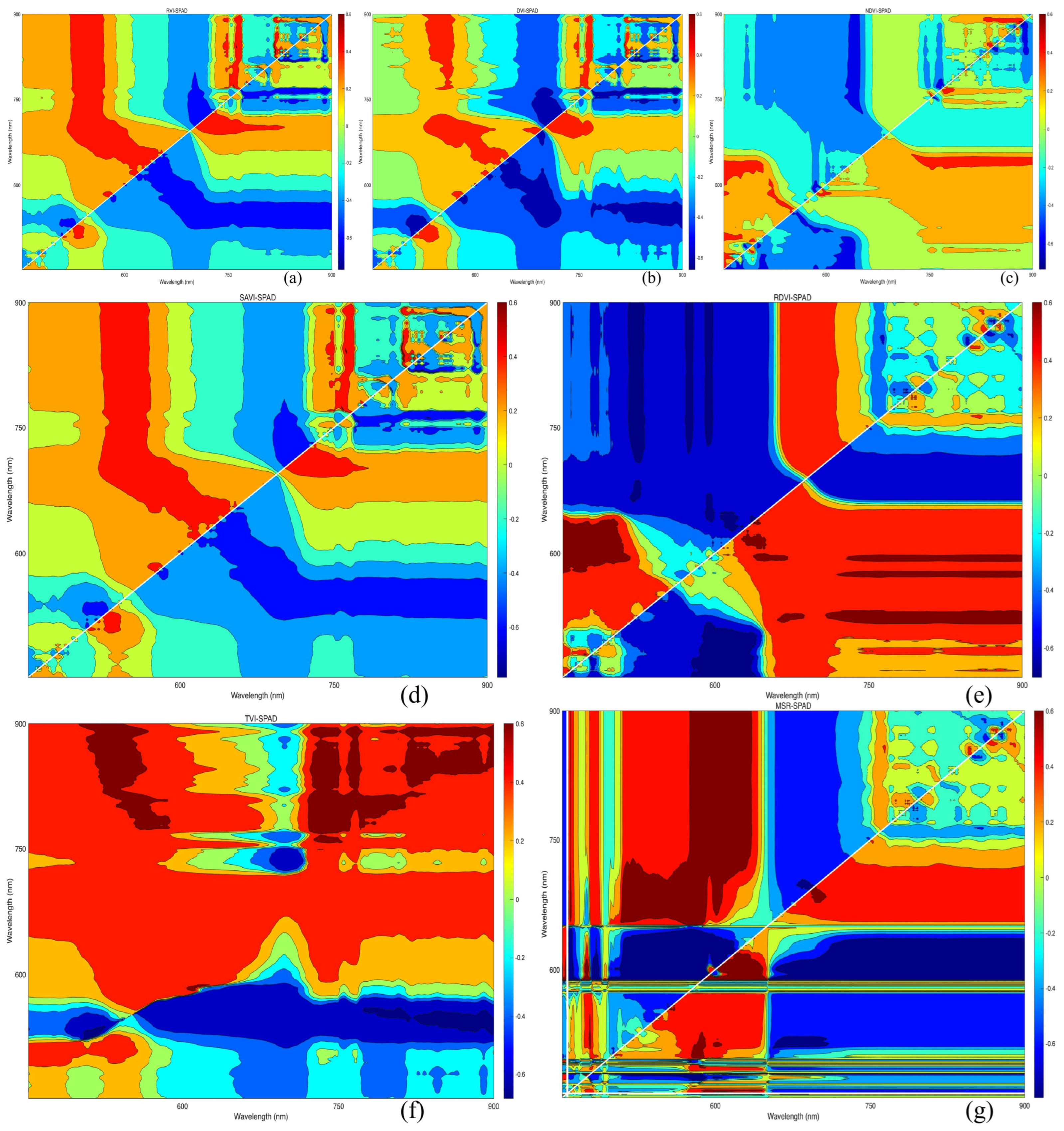
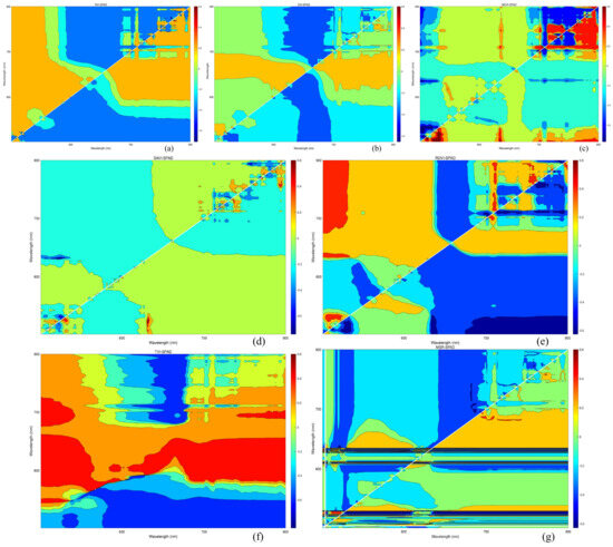
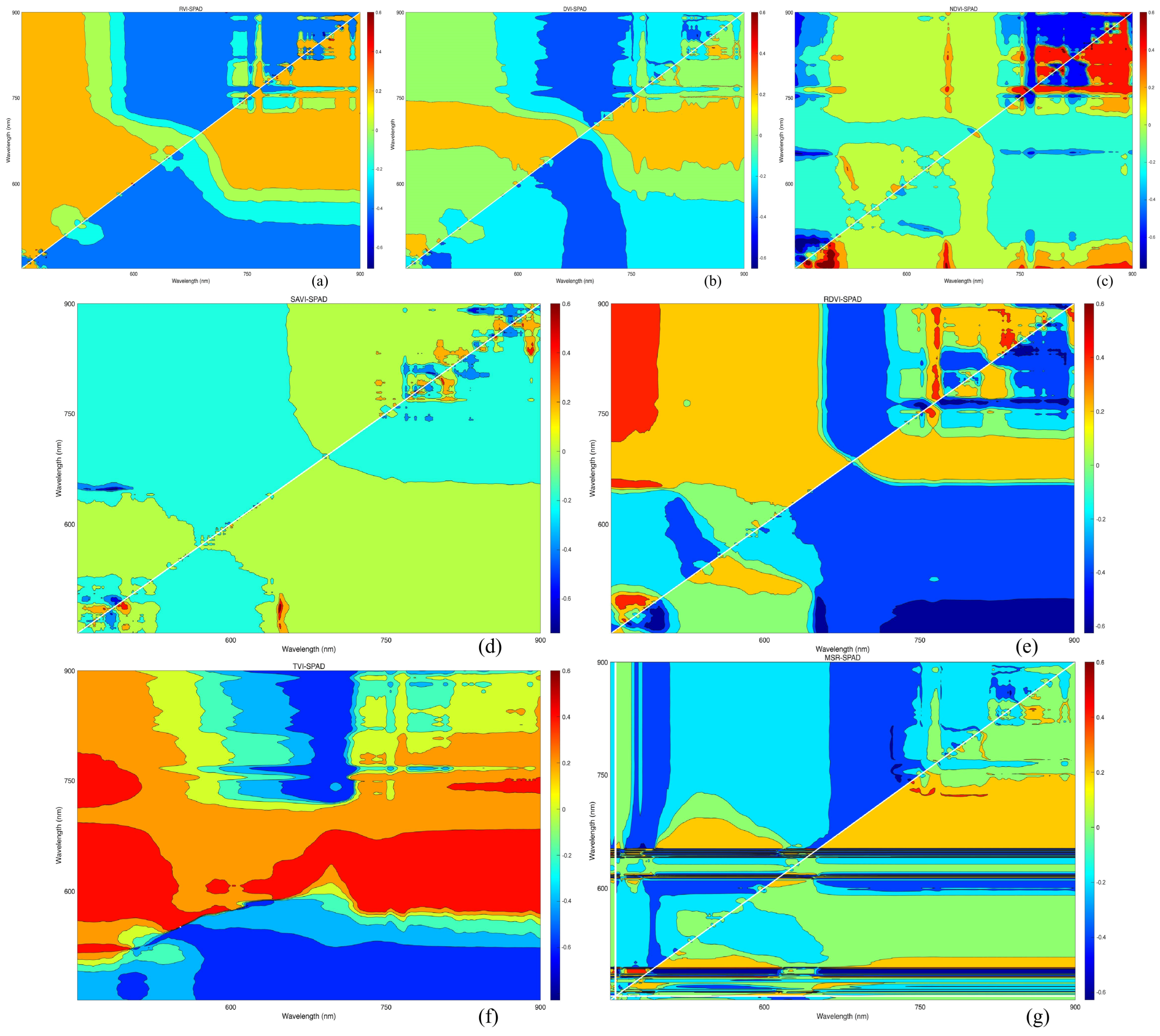
To fully explore the fine spectral features of hyperspectral data and the synergistic effects between bands, this study uses the Correlation Matrix Method to calculate all possible two-band combinations within the 400–950 nm range for the preprocessed spectral data from two phenological periods. Based on the selected seven classic vegetation indices: RVI, DVI, NDVI, SAVI, RDVI, TVI, and MSR, the correlation between these indices and SPAD values is analyzed. The wavelengths corresponding to the maximum correlation coefficient, $R_i$ and $R_j$, are selected as the optimal wavelength combination. The calculated spectral index values are considered the optimal spectral indices most strongly correlated with chlorophyll, which will be used to construct the chlorophyll content estimation model for the apple tree canopy leaves. The correlation coefficients between the spectral indices and SPAD values for different phenological periods, as well as the bands and optimal spectral indices, are shown in Table 2. Figure 5 and Figure 6 present the correlation contour maps between the optimal spectral indices (RVI, DVI, NDVI, SAVI, RDVI, TVI, and mSR) and the measured SPAD values for different phenological periods. Any point in the figures represents the absolute value of the correlation coefficient between the two wavelengths of the optimal spectral index and chlorophyll.

Table 2. Wavelength Positions and Combinations of Optimal Spectral Indices for Different Phenological Periods.

Phenological Stage	Spectral Index	Maximum Correlation Coefficient	Wavelength/$({\mathit{R}}_{\mathit{i}},{\mathit{R}}_{\mathit{j}})$	Optimal Portfolio
Period of physiological fruit drop	RVI	0.770	686,669	RVI, SAVI, MSR
	DVI	0.654	697,667
	NDVI	0.731	737,735
	SAVI	0.785	688,669
	RDVI	0.699	577,578
	TVI	0.644	636,667
	mSR	0.748	628,623
Fruit enlargement stage	RVI	0.704	704,710	RVI, NDVI, SAVI
	DVI	0.650	633,629
	NDVI	0.766	714,716
	SAVI	0.738	538,698
	RDVI	0.624	625,624
	TVI	0.656	577,552
	mSR	0.668	764,610

Figure 5. Correlation matrix between optimal spectral indices and SPAD values during the physiological fruit drop stage. Subfigures (a–g) represent RVI, DVI, NDVI, SAVI, RDVI, TVI, and mSR, respectively. The diagonal white lines indicate the axes of symmetry for the correlation coefficients.

Figure 6. Correlation matrix between optimal spectral indices and SPAD values during the fruit expansion stage. Subfigures (a–g) represent RVI, DVI, NDVI, SAVI, RDVI, TVI, and mSR, respectively. The diagonal white lines indicate the axes of symmetry for the correlation coefficients.

The color scale represents the value of the correlation coefficient (r). Warmer colors (e.g., red and orange) indicate a strong positive correlation between the spectral indices and SPAD values, whereas cooler colors (e.g., blue) indicate a weak or negative correlation. The distinct deep red regions specifically highlight the optimal wavelength combinations with the highest correlation accuracy.

During the physiological fruit drop period, the spectral index with the highest correlation coefficient to SPAD values is SAVI, with a correlation coefficient of 0.785. The corresponding wavelength combination is 688 nm and 669 nm. The other spectral indices are ranked by their maximum correlation coefficients in descending order as follows:

RVI (r686, r669) > MSR (r628, r623) > NDVI (r737, r735) > RDVI (r577, r578) > DVI (r697, r667) > TVI (r636, r667).

During the fruit enlargement period, the spectral index with the highest correlation coefficient to SPAD values is NDVI, with a correlation coefficient of 0.766. The corresponding wavelength combination is 714 nm and 716 nm. The results of the other spectral indices are ranked by their maximum correlation coefficients from high to low as follows:

SAVI (r538, 698) > RVI (r704, r710) > MSR (r764, 610) > TVI (r577, r552) > DVI (r633, r629) > RDVI (r625, r624).

According to previous studies, using the correlation matrix method to combine bands with high correlation can effectively reduce uncertainty, thereby improving the accuracy of SPAD value inversion models for different phenological periods. To construct a high-precision and physically interpretable inversion model, this study sets a feature selection threshold of |r| > 0.7. During the physiological fruit drop period, the final selected spectral indices are SAVI (r688, r669), RVI (r686, r669), MSR (r628, r623), and NDVI (r737, r735). During the fruit enlargement period, the final selected spectral indices are NDVI (r714, r716), SAVI (r538, r698), and RVI (r704, r710).

In summary, this study extracted SPA feature bands based on physical absorption characteristics and optimal spectral indices based on the synergistic effects between bands. These two types of features were used as model inputs to construct the SPAD collaborative inversion model and compare its modeling accuracy.

3.2. Machine Learning-Based SPAD Estimation Model Construction and Evaluation

3.2.1. Model Parameter Optimization Results

According to the optimization strategy set in this study, grid search (GS) and chaotic optimization (CEO) algorithms were used to optimize the model parameters for different input features and phenological stages. The experimental results show that the CEO algorithm demonstrates stronger global search ability than the traditional GS method when optimizing the hyperparameter space of LSSVM, effectively improving the model’s stability on the validation set.

The key parameter configurations for each model at their optimal state are shown in Table 3. For example, in the physiological fruit drop stage, the optimal penalty factor (C) for the CEO-LSSVM model constructed with spectral indices was 15.24, and the kernel parameter (r) was 0.032. These specific parameter values ensure that the model can balance learning accuracy and generalization performance in subsequent SPAD inversion tasks.

Table 3. Optimal hyperparameter configurations for different SPAD estimation models.

Phenological Stage	Algorithm	Penalty Factor ($\mathit{\gamma }$)	Kernel Parameter ($\mathit{\sigma }$)
Period of physiological fruit drop	SVM	10.00	0.100
	LSSVM	12.00	0.050
	CEO	15.24	0.032
Fruit enlargement stage	SVM	10.00	0.100
	LSSVM	12.00	0.050
	CEO	15.24	0.032

3.2.2. Comparison and Analysis of Modeling Accuracy with Different Input Features

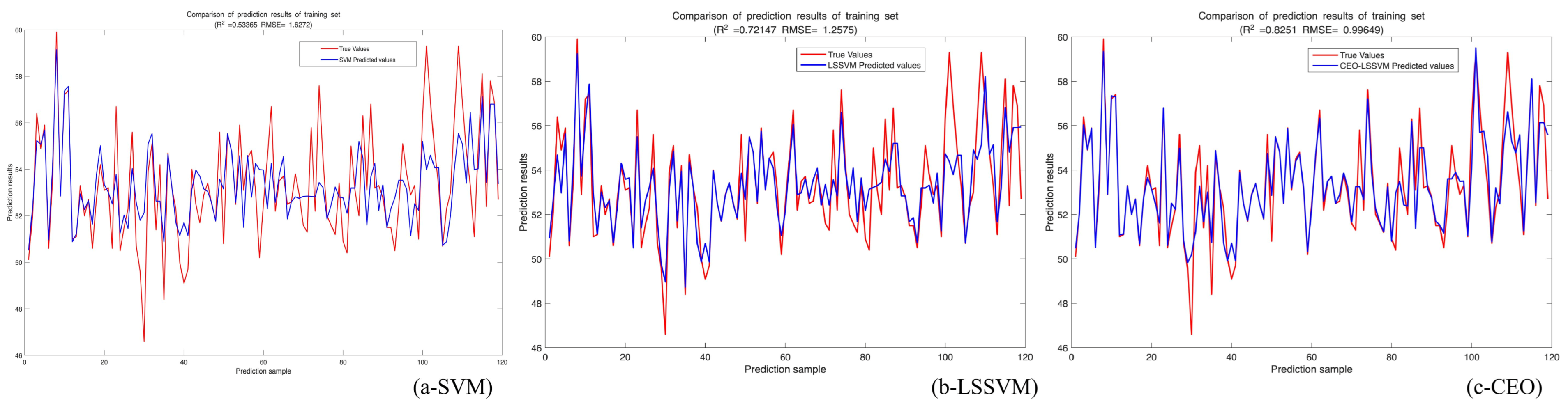
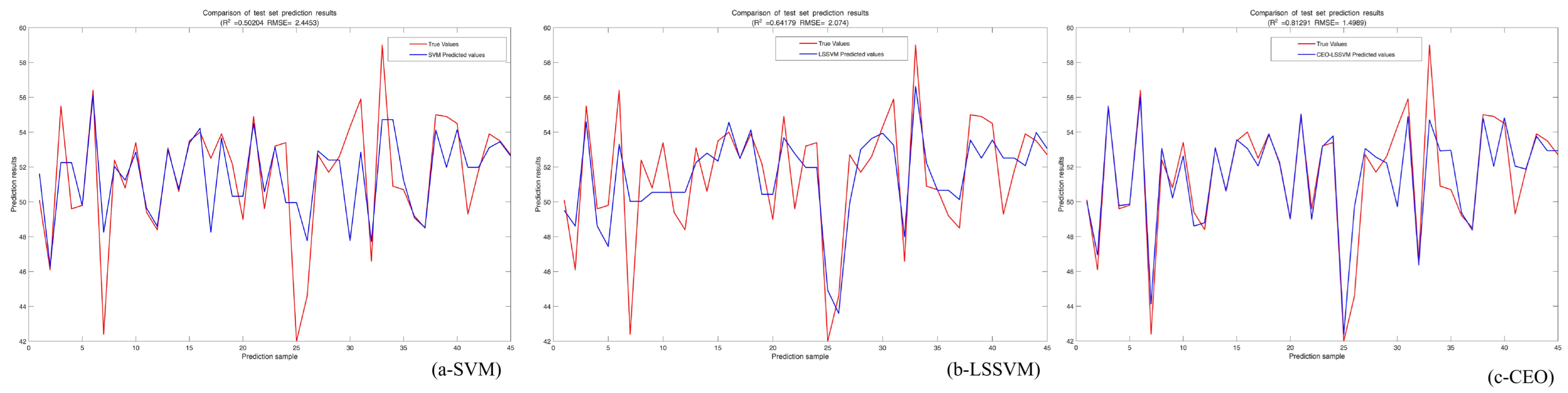
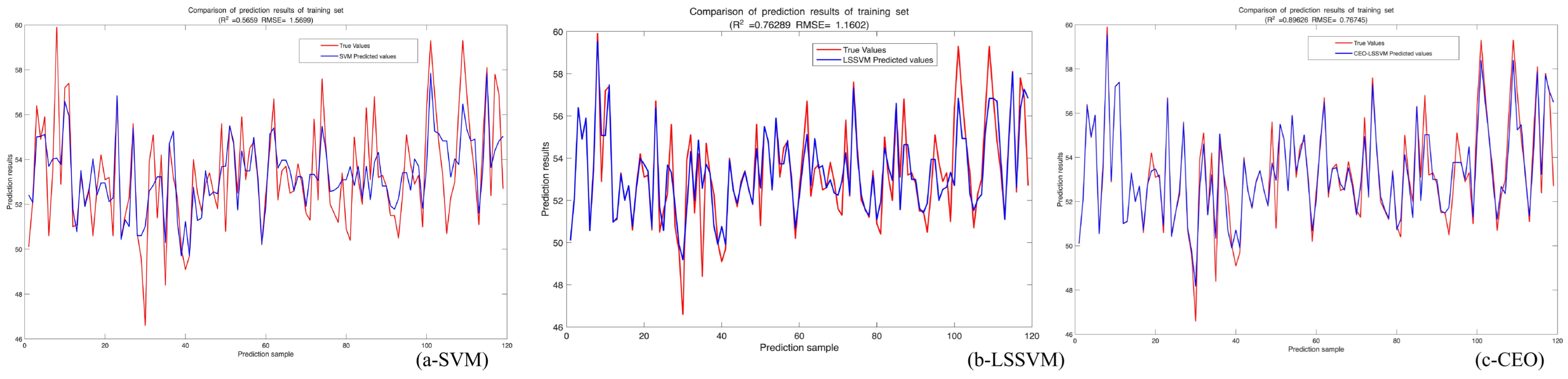
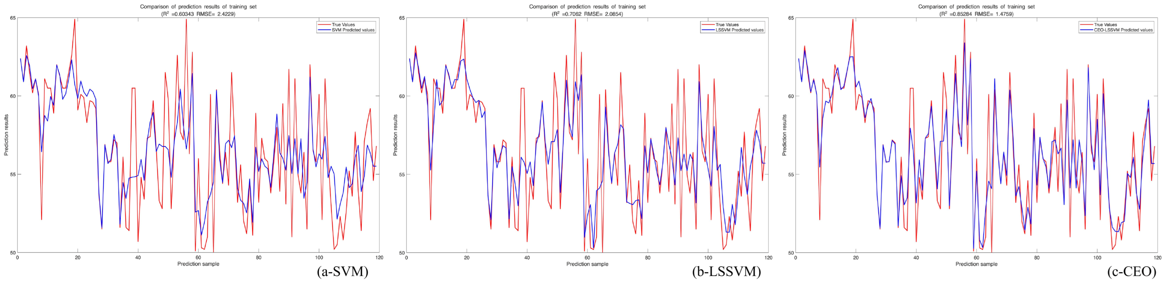
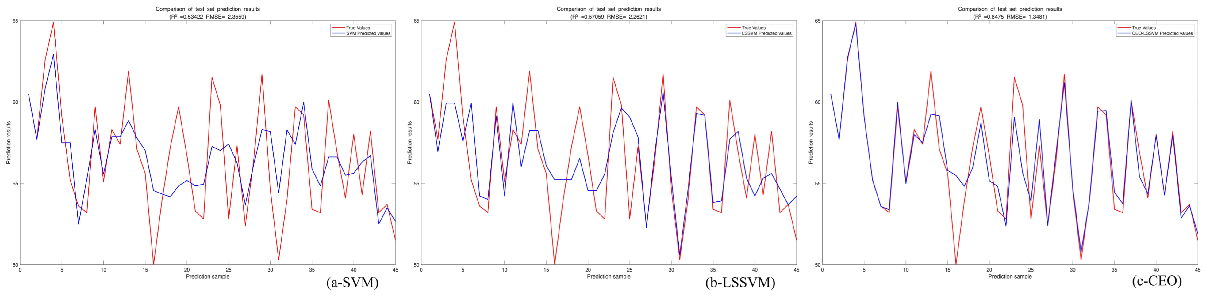
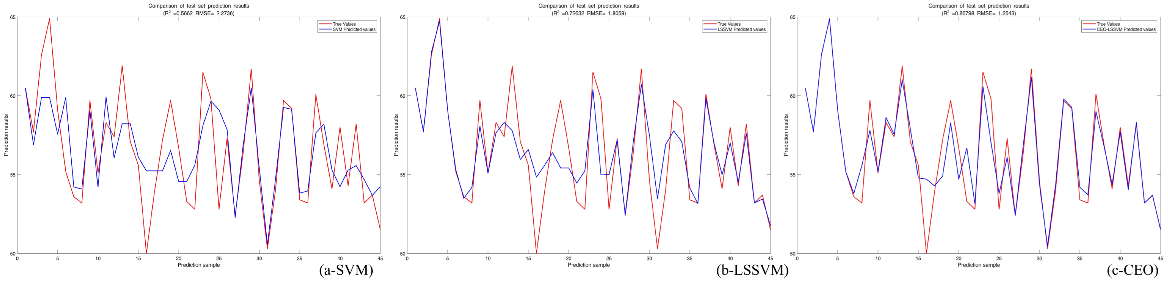
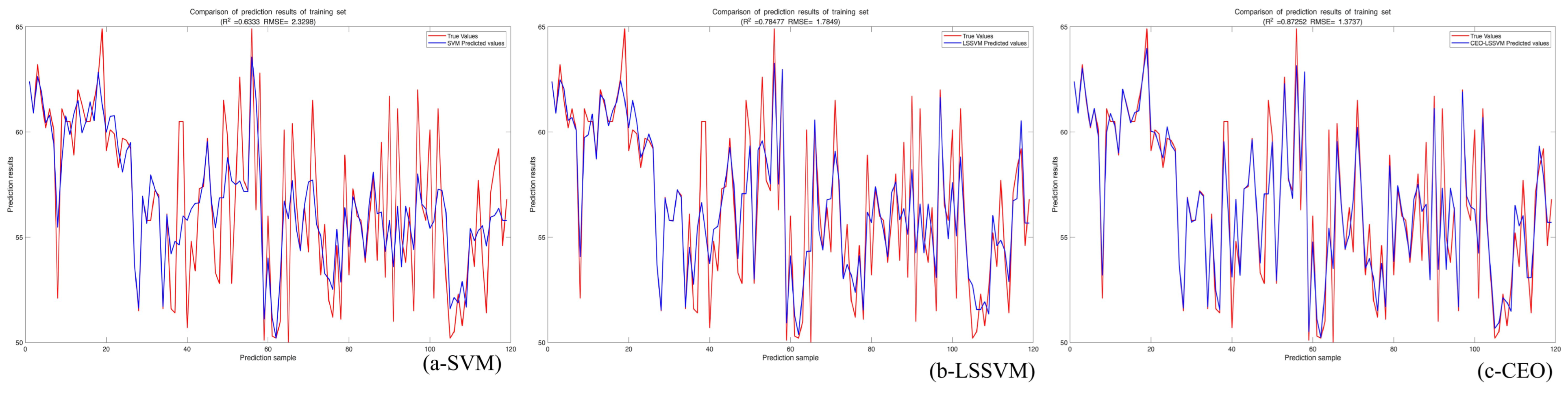
In order to comprehensively assess the impact of different input variables on the accuracy of SPAD value inversion, this study constructed three regression prediction models—SVM, LSSVM, and CEO-LSSVM—using the optimal spectral indices (4 indices for the physiological fruit drop stage and 3 indices for the fruit enlargement stage) and the features extracted by the SPA algorithm (6 features for the physiological fruit drop stage and 5 features for the fruit enlargement stage) as input variables. The performance of each model on the training and test sets during different growth stages is shown in Table 4 and Figure 7, Figure 8, Figure 9, Figure 10, Figure 11, Figure 12, Figure 13 and Figure 14.

Table 4. Performance comparison of SPAD estimation models based on different input features.

Period of physiological fruit drop	Input Variables	Model	R2		RMSE
			Training Set	Test Set	Training Set	Test Set
	Spectral Index	SVM	0.5659	0.5166	1.5699	2.4093
		LSSVM	0.7629	0.7585	1.1602	1.7030
		CEO-LSSVM	0.8963	0.8509	0.7675	1.3378
	SPA	SVM	0.5337	0.5020	1.6272	2.4453
		LSSVM	0.7215	0.6418	1.2575	2.0740
		CEO-LSSVM	0.8251	0.8129	0.9965	1.4989
Fruit enlargement stage	Input variables	Model	R2		RMSE
			training set	Test set	training set	Test set
	Spectral Index	SVM	0.6333	0.5662	2.3298	2.2736
		LSSVM	0.7848	0.7263	1.7849	1.8059
		CEO-LSSVM	0.8725	0.8679	1.3737	1.2543
	SPA	SVM	0.6034	0.5342	2.4229	2.3559
		LSSVM	0.7062	0.5707	2.0854	2.2621
		CEO-LSSVM	0.8528	0.8475	1.4759	1.3481

Figure 7. Fitting results of the training set for SPAD estimation models based on SPA features during the physiological fruit drop stage.

Figure 8. Fitting results of the test set for SPAD estimation models based on SPA features during the physiological fruit drop stage.

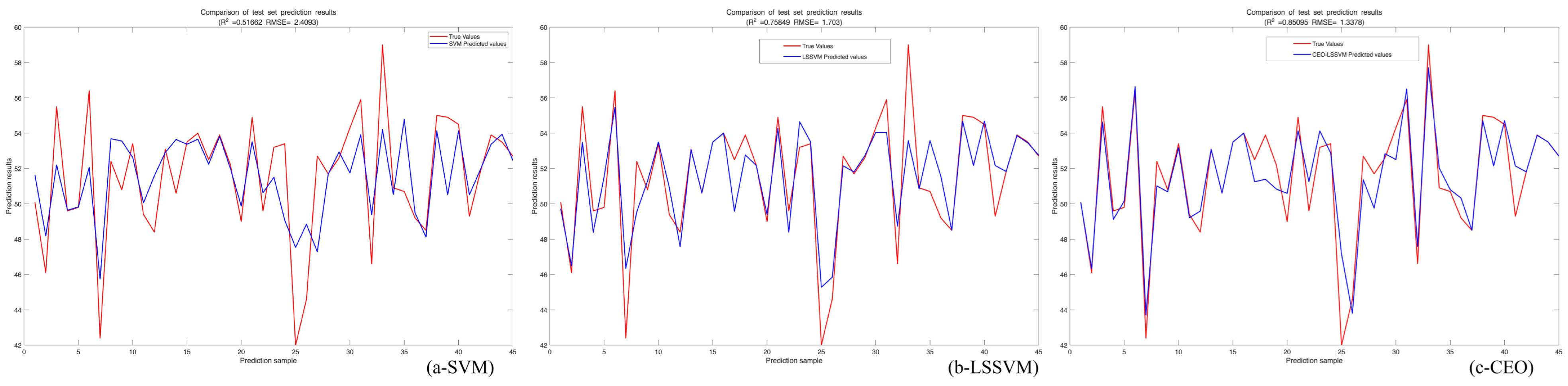
Figure 9. Fitting results of the test set for SPAD estimation models based on optimal spectral indices during the physiological fruit drop stage.

Figure 10. Fitting results of the training set for SPAD estimation models based on optimal spectral indices during the physiological fruit drop stage.

Figure 11. Fitting results of SPAD estimation models on the training set during fruit expansion stage based on SPA features.

Figure 12. Fitting results of SPAD estimation models on the test set during fruit expansion stage based on SPA features.

Figure 13. Fitting results of the test set for SPAD estimation models based on optimal spectral indices during the fruit expansion stage.

Figure 14. Fitting results of the training set for SPAD estimation models based on optimal spectral indices during the fruit expansion stage.

The results show that the CEO-LSSVM model exhibited the best predictive performance in all test combinations. For example, in the physiological fruit drop stage, the CEO-LSSVM model constructed with spectral indices achieved a coefficient of determination (R²) of 0.851 and a root mean square error (RMSE) of 1.338 on the test set, significantly outperforming the non-optimized LSSVM (R² = 0.758) and standard SVM (R² = 0.517). This demonstrates that the introduction of the chaotic optimization algorithm effectively overcomes the limitations of traditional machine learning models, which are prone to local optima, thereby accurately capturing the complex nonlinear mapping relationship between spectral data and chlorophyll content.

A comparison between the two types of input features reveals that models based on a few spectral indices generally perform better or are comparable to models based on SPA feature bands. In the fruit enlargement stage, the CEO-LSSVM model with only 3 spectral indices achieved an R² of 0.868 on the test set, which is better than the model based on 5 SPA bands (R² = 0.848). In the physiological fruit drop stage, the spectral index model (R² = 0.851) also demonstrated stronger explanatory power than the SPA model (R² = 0.813). This suggests that spectral indices, through cooperative operations between bands (such as normalization and ratio calculation), can more effectively suppress environmental background noise and canopy structural interference. Moreover, the reduction in the number of variables significantly lowers the model’s computational complexity and the risk of overfitting.

Overall, across both phenological stages, the inversion accuracy during the fruit enlargement stage was generally higher than in the physiological fruit drop stage (with the highest test set R² values of 0.868 and 0.851, respectively). This is attributed to the maturity of leaf structure during the enlargement stage, where chlorophyll content tends to stabilize, thus reducing the uncertainty in spectral responses. However, the CEO-LSSVM model maintained high robustness in both stages, demonstrating its potential for monitoring SPAD values throughout the entire growth cycle of apple leaves.

4. Discussion

4.1. Mechanism of Spectral Response Heterogeneity Driven by Phenological Evolution

The results of this study indicate that there are significant differences in the optimal spectral band combinations and spectral index types for apple leaf SPAD values between the physiological fruit drop stage and the fruit expansion stage. This phenomenon is essentially attributed to the synergistic regulatory effect of canopy structure and leaf physiological status on spectral response mechanisms across different phenological stages [37].

During the physiological fruit drop stage, apple trees are in a phase of rapid new shoot growth and young fruit development. The canopy is not yet fully closed, and interference from the background (branches, soil, and weeds) on canopy reflectance is relatively pronounced. Concurrently, demands for nitrogen and water peak during this stage; while chlorophyll content rises rapidly, it has not yet reached a stable level [38,39]. Consequently, the characteristic bands selected by the SPA algorithm (587 nm, 698–730 nm, 799 nm, and 973 nm) reflect this complex physiological state. Specifically, the 587 nm band on the descending slope of the green peak captures subtle pigment changes [40], while the 973 nm band, located in a water vapor absorption region, indicates a strong physiological covariation between leaf water content and photosynthetic pigment accumulation during this rapid growth phase [41]. This suggests that variations in SPAD values during this stage are collectively influenced by pigment absorption, water status, and structural characteristics.

During the fruit expansion stage, as leaves fully expand and the canopy tends toward high density, background interference weakens, and chlorophyll content becomes relatively stable. Specifically, the SPA algorithm selected five characteristic bands: 529 nm, 696 nm, 713 nm, 808 nm, and 894 nm. The physical interpretation of these bands is supported by distinct physiological mechanisms. First, the 529 nm band is located near the green reflection peak. Previous studies have demonstrated that as leaf chlorophyll content increases, absorption in the red region tends to saturate, whereas reflectance in the green region maintains high sensitivity to chlorophyll variation [40,42]. Second, the 696 nm and 713 nm bands fall within the red-edge region, which is known to be highly sensitive to photosynthetic activity and pigment concentration [41]. Third, the 808 nm and 894 nm bands are situated in the near-infrared plateau, where reflectance is primarily governed by the internal scattering of leaf cell structures and canopy thickness rather than pigment absorption [43]. The exclusion of water-sensitive bands (e.g., ~970 nm) compared to the previous stage indicates that the spectral response mechanism has shifted from being dominated by water and background factors to centering on chlorophyll absorption and canopy structural characteristics. This result aligns with previous findings that the combination of green-peak and red-edge bands provides a robust basis for SPAD estimation under high-biomass conditions [44,45].

4.2. Robustness Analysis of Structured Spectral Indices in Feature Extraction

The results of this study indicate that the inversion models built with a few spectral indices generally have superior or comparable prediction accuracy to those based on feature bands extracted using the SPA method. For example, during the physiological fruit drop stage, the CEO-LSSVM model based on spectral indices achieved an R² of 0.896 on the test set, significantly higher than the 0.813 obtained with SPA input. This result validates that in hyperspectral inversion, effectively extracting core information highly coupled with the target variable is key to enhancing the robustness of the model.

From a physical mechanism perspective, spectral indices perform a “physically inspired feature enhancement” through mathematical construction. During stages of lower canopy cover, indices such as SAVI effectively compensate for the nonlinear interference of background reflectance by introducing a soil adjustment factor, thus suppressing background noise [38,46]. The ratio or normalization structures used in spectral indices (e.g., NDVI-type indices) can effectively eliminate brightness fluctuations and shadow effects caused by canopy structure, fruit occlusion, or microtopography.

In contrast, although the SPA algorithm reduces data redundancy by selecting bands with minimal collinearity, it essentially extracts linear subsets of the original reflectance data [23]. In the complex canopy environment of fruit trees, individual bands are easily affected by observation geometry (BRDF) and environmental noise [47,48]. When the sample size is limited, inputting too many bands may lead to overfitting, resulting in a decline in model generalization capability. Spectral indices, by compressing multi-band information into a low-dimensional space, not only significantly enhance the information but also improve the model’s sensitivity to physiological dynamic changes through their structured mathematical form [49,50]. This “low-dimensional, high-efficiency” feature extraction model provides an optimal mathematical pathway for establishing robust models across phenological stages.

4.3. Performance Advantages of the CEO-LSSVM Model in Modeling Complex Nonlinear Relationships

The consistent results of this study indicate that the CEO-LSSVM model significantly outperforms traditional SVM and non-optimized LSSVM models in terms of prediction performance across different phenological stages and input feature combinations. According to the data in Table 3, the model accuracy shows a clear ranking: CEO-LSSVM > LSSVM > SVM.

While the use of spectral indices provides a physically robust data foundation, the modeling approach remains the critical determinant of prediction accuracy in complex field environments. Existing modeling approaches, such as traditional SVM and standard LSSVM, face significant limitations when handling agricultural in situ hyperspectral data. These models rely heavily on the precise configuration of hyperparameters (e.g., regularization parameters and kernel width) to model highly nonlinear relationships [51,52]. However, field canopy spectra are characterized by high noise levels caused by uneven lighting, weed backgrounds, and complex tree structures. Consequently, the objective function surfaces of these models become multi-peaked and non-convex. Traditional parameter tuning methods, such as grid search or random search, typically use fixed step sizes and lack heuristic mechanisms. As a result, they are prone to falling into local optima, leading to poor generalization and “underfitting” on the test set—evidenced by the SVM’s RMSE reaching as high as 2.409 in this study.

The proposed CEO-LSSVM framework specifically overcomes these shortcomings through its advanced algorithmic structure. During the physiological fruit drop stage, the CEO-LSSVM model achieved an R² of 0.896, representing improvements of 73.3% and 18.2% over SVM (0.517) and LSSVM (0.758), respectively. This performance boost is primarily attributed to the global optimization capability of the Chaos Game Optimization (CEO) algorithm. By introducing chaotic mapping, the algorithm ensures population diversity in the early search stages, preventing premature convergence. In later stages, it utilizes a game strategy to deeply explore the parameter space, automatically identifying the global optimal hyperparameters [53,54]. This mechanism effectively resolves the trade-off between “underfitting” and “overfitting,” allowing the CEO-LSSVM to maintain a low and stable RMSE (1.25–1.49) even during the fruit enlargement stage, where high chlorophyll content typically causes “absorption saturation.” This robust performance demonstrates the high engineering value of the CEO-LSSVM algorithm in overcoming the instability inherent in traditional machine learning approaches.

5. Conclusions

Comparison revealed that models constructed based on a few spectral indices exhibited superior generalization ability compared to those based on characteristic bands selected by SPA. While spectral indices based on physical principles are more resistant to multiplicative noise than statistical band selection methods (such as SPA), high-quality features alone are insufficient for precise monitoring in complex environments. The main challenge lies in the modeling methodology used to interpret these features. Traditional regression models, due to their sensitivity to hyperparameter settings and susceptibility to becoming trapped in local optima, often fail to capture the complex nonlinear relationships in field data. This study addressed these limitations by proposing a SPAD value inversion framework based on the Chaos Evolution Optimization (CEO-LSSVM) algorithm. The main conclusions are as follows:

During the physiological fruit drop stage, SPAD inversion was influenced by water status and structural characteristics (optimal indices: SAVI, RVI, MSR, NDVI). In the fruit expansion stage, key features converged toward pigment-sensitive indices (NDVI, SAVI, RVI). This confirms that while features shift with phenology, the modeling framework must be robust enough to adapt to these changes.

In all tested scenarios, the CEO-LSSVM significantly outperformed traditional SVM and LSSVM models. During the physiological fruit drop stage, the R² on the test set improved by up to 0.334 and 0.171 compared to SVM and LSSVM, respectively. Crucially, the model maintained test set R² values consistently above 0.85 during the fruit expansion stage.

The study proves that the CEO-LSSVM framework effectively overcomes the “local optima” and “overfitting” issues common in standard machine learning models. By utilizing chaotic mapping for global search, the algorithm accurately pinpoints the optimal hyperparameters of the LSSVM, ensuring stability even with noisy, nonlinear field data. Consequently, this study provides a robust technical solution for precision nutrient monitoring that is superior to traditional modeling approaches.

References

- Ta, N.; Chang, Q.; Zhang, Y. Estimation of apple tree leaf chlorophyll content based on machine learning methods. Remote Sens. 2021, 13, 3902. [Google Scholar] [CrossRef] [Scilit]
- Zhang, Y.; Chang, Q.; Chen, Y.; Liu, Y.; Jiang, D.; Zhang, Z. Hyperspectral estimation of chlorophyll content in apple tree leaf based on feature band selection and the CatBoost model. Agronomy 2023, 13, 2075. [Google Scholar] [CrossRef] [Scilit]
- Liang, S.; Zhao, G.-X.; Zhu, X.-C. Hyperspectral estimation models of chlorophyll content in apple leaves. Spectrosc. Spectr. Anal. 2012, 32, 1367–1370. [Google Scholar]
- Mu, W.; Duan, X.; Wang, Q.; Wei, X.; Wei, K.; Li, Y.; Guo, X. Effect of Drip Irrigation, N, K, and Zn Coupling on P n of Densely Cultivated Apple on Dwarf Rootstock in Xinjiang, China. Agronomy 2023, 13, 1082. [Google Scholar] [CrossRef] [Scilit]
- Cao, H.; Wang, H.; Li, Y.; Hamani, A.K.M.; Zhang, N.; Wang, X.; Gao, Y. Evapotranspiration partition and dual crop coefficients in apple orchard with dwarf stocks and dense planting in arid region, Aksu oasis, southern Xinjiang. Agriculture 2021, 11, 1167. [Google Scholar] [CrossRef] [Scilit]
- Wang, J.; Zhang, Y.; Han, F.; Shi, Z.; Zhao, F.; Zhang, F.; Pan, W.; Zhang, Z.; Cui, Q. Estimation of Canopy Chlorophyll Content of Apple Trees Based on UAV Multispectral Remote Sensing Images. Agriculture 2025, 15, 1308. [Google Scholar] [CrossRef] [Scilit]
- Fu, Y.; Yang, G.; Pu, R.; Li, Z.; Li, H.; Xu, X.; Song, X.; Yang, X.; Zhao, C. An overview of crop nitrogen status assessment using hyperspectral remote sensing: Current status and perspectives. Eur. J. Agron. 2021, 124, 126241. [Google Scholar] [CrossRef] [Scilit]
- Fu, Y.; Yang, G.; Li, Z.; Li, H.; Li, Z.; Xu, X.; Song, X.; Zhang, Y.; Duan, D.; Zhao, C. Progress of hyperspectral data processing and modelling for cereal crop nitrogen monitoring. Comput. Electron. Agric. 2020, 172, 105321. [Google Scholar] [CrossRef] [Scilit]
- Wu, C.; Niu, Z.; Tang, Q.; Huang, W. Estimating chlorophyll content from hyperspectral vegetation indices: Modeling and validation. Agric. For. Meteorol. 2008, 148, 1230–1241. [Google Scholar] [CrossRef] [Scilit]
- Sonobe, R.; Yamashita, H.; Mihara, H.; Morita, A.; Ikka, T. Estimation of leaf chlorophyll a, b and carotenoid contents and their ratios using hyperspectral reflectance. Remote Sens. 2020, 12, 3265. [Google Scholar] [CrossRef] [Scilit]
- Xiao, Q.; Tang, W.; Zhang, C.; Zhou, L.; Feng, L.; Shen, J.; Yan, T.; Gao, P.; He, Y.; Wu, N. Spectral preprocessing combined with deep transfer learning to evaluate chlorophyll content in cotton leaves. Plant Phenomics 2022, 2022, 9813841. [Google Scholar] [CrossRef] [Scilit]
- Yue, J.; Feng, H.; Yang, G.; Li, Z. A comparison of regression techniques for estimation of above-ground winter wheat biomass using near-surface spectroscopy. Remote Sens. 2018, 10, 66. [Google Scholar] [CrossRef] [Scilit]
- Zhang, J.; Fu, P.; Meng, F.; Yang, X.; Xu, J.; Cui, Y. Estimation algorithm for chlorophyll-a concentrations in water from hyperspectral images based on feature derivation and ensemble learning. Ecol. Inform. 2022, 71, 101783. [Google Scholar] [CrossRef] [Scilit]
- Cui, B.; Zhao, Q.; Huang, W.; Song, X.; Ye, H.; Zhou, X. A new integrated vegetation index for the estimation of winter wheat leaf chlorophyll content. Remote Sens. 2019, 11, 974. [Google Scholar] [CrossRef] [Scilit]
- Li, C.; Zhu, X.; Wei, Y.; Cao, S.; Guo, X.; Yu, X.; Chang, C. Estimating apple tree canopy chlorophyll content based on Sentinel-2A remote sensing imaging. Sci. Rep. 2018, 8, 3756. [Google Scholar] [CrossRef] [Scilit] [PubMed]
- Ding, D.; Yu, H.; Yin, Y.; Yuan, Y.; Li, Z.; Li, F. Determination of Chlorophyll and Hardness in Cucumbers by Raman Spectroscopy with Successive Projections Algorithm (SPA)–Extreme Learning Machine (ELM). Anal. Lett. 2023, 56, 1216–1228. [Google Scholar] [CrossRef] [Scilit]
- Gao, J.; Zhang, Z. Study on deep learning model for online estimation of chlorophyll content based on near ground multispectral feature bands. IEEE Access 2022, 10, 132183–132192. [Google Scholar] [CrossRef] [Scilit]
- Zhang, Y.; Zheng, L.; Li, M.; Deng, X.; Ji, R. Predicting apple sugar content based on spectral characteristics of apple tree leaf in different phenological phases. Comput. Electron. Agric. 2015, 112, 20–27. [Google Scholar] [CrossRef] [Scilit]
- Jiang, C.; Cheng, Y.; Li, Y.; Peng, L.; Dong, G.; Lai, N.; Geng, Q. Phenology-Aware Machine Learning Framework for Chlorophyll Estimation in Cotton Using Hyperspectral Reflectance. Remote Sens. 2025, 17, 2713. [Google Scholar] [CrossRef] [Scilit]
- Arseneault, M.H.; Cline, J.A. A review of apple preharvest fruit drop and practices for horticultural management. Sci. Hortic. 2016, 211, 40–52. [Google Scholar] [CrossRef] [Scilit]
- Peng, X. Study on Apple Marketing Model Based on Modern Aksu Region in Xinjiang. In Proceedings of the 2017 5th International Education, Economics, Social Science, Arts, Sports and Management Engineering Conference (IEESASM 2017), Qingdao, China, 28–29 December 2017; Atlantis Press: Dordrecht, The Netherlands, 2017; p. 4. [Google Scholar]
- Chen, J.; Bai, T.; Zhang, N.; Zhu, L.; Zhang, X. Hyperspectral detection of sugar content for sugar-sweetened apples based on sample grouping and SPA feature selecting methods. Infrared Phys. Technol. 2022, 125, 104240. [Google Scholar] [CrossRef] [Scilit]
- Zhang, J.; Rivard, B.; Rogge, D. The successive projection algorithm (SPA), an algorithm with a spatial constraint for the automatic search of endmembers in hyperspectral data. Sensors 2008, 8, 1321–1342. [Google Scholar] [CrossRef] [Scilit]
- Bannari, A.; Morin, D.; Bonn, F.; Huete, A. A review of vegetation indices. Remote Sens. Rev. 1995, 13, 95–120. [Google Scholar] [CrossRef] [Scilit]
- Fang, W.; Zhu, H.; Li, S.; Ding, H.; Bi, R. Rapid identification of main vegetation types in the Lingkong mountain nature reserve based on multi-temporal modified vegetation indices. Sensors 2023, 23, 659. [Google Scholar] [CrossRef] [Scilit]
- Pettorelli, N.; Ryan, S.; Mueller, T.; Bunnefeld, N.; Jędrzejewska, B.; Lima, M.; Kausrud, K. The Normalized Difference Vegetation Index (NDVI): Unforeseen successes in animal ecology. Clim. Res. 2011, 46, 15–27. [Google Scholar] [CrossRef] [Scilit]
- Rondeaux, G.; Steven, M.; Baret, F. Optimization of soil-adjusted vegetation indices. Remote Sens. Environ. 1996, 55, 95–107. [Google Scholar] [CrossRef] [Scilit]
- Chen, J.M. Evaluation of vegetation indices and a modified simple ratio for boreal applications. Can. J. Remote Sens. 1996, 22, 229–242. [Google Scholar] [CrossRef] [Scilit]
- Mutanga, O.; Skidmore, A.K. Narrow band vegetation indices overcome the saturation problem in biomass estimation. Int. J. Remote Sens. 2004, 25, 3999–4014. [Google Scholar] [CrossRef] [Scilit]
- Gholami, R.; Fakhari, N. Support vector machine: Principles, parameters, and applications. In Handbook of Neural Computation; Elsevier: Amsterdam, The Netherlands, 2017; pp. 515–535. [Google Scholar]
- Xu, L.; Hao, G.; Li, S.; Song, F.; Zhao, Y.; Guo, P. Prediction and sensitivity analysis of chlorophyll a based on a support vector machine regression algorithm. Environ. Monit. Assess. 2023, 195, 698. [Google Scholar] [CrossRef] [Scilit]
- Suykens, J.A.; Lukas, L.; Van Dooren, P.; De Moor, B.; Vandewalle, J. Least squares support vector machine classifiers: A large scale algorithm. In Proceedings of the European Conference on Circuit Theory and Design, ECCTD, Stresa, Italy, 29 August–2 September 1999; pp. 839–842. [Google Scholar]
- Pelckmans, K.; Suykens, J.A.; Van Gestel, T.; De Brabanter, J.; Lukas, L.; Hamers, B.; De Moor, B.; Vandewalle, J. LS-SVMlab: A matlab/c toolbox for least squares support vector machines. Tutorial. KULeuven-ESAT 2002, 142. [Google Scholar]
- Talatahari, S.; Azizi, M. Chaos game optimization: A novel metaheuristic algorithm. Artif. Intell. Rev. 2021, 54, 917–1004. [Google Scholar] [CrossRef] [Scilit]
- Kennard, R.W.; Stone, L.A. Computer Aided Design of Experiments. Technometrics 2012, 11, 137–148. [Google Scholar] [CrossRef]
- Li, D.; Hu, Q.; Ruan, S.; Liu, J.; Zhang, J.; Hu, C.; Liu, Y.; Dian, Y.; Zhou, J. Utilizing hyperspectral reflectance and machine learning algorithms for non-destructive estimation of chlorophyll content in citrus leaves. Remote Sens. 2023, 15, 4934. [Google Scholar] [CrossRef] [Scilit]
- Soudani, K.; Hmimina, G.; Delpierre, N.; Pontailler, J.-Y.; Aubinet, M.; Bonal, D.; Caquet, B.; De Grandcourt, A.; Burban, B.; Flechard, C. Ground-based Network of NDVI measurements for tracking temporal dynamics of canopy structure and vegetation phenology in different biomes. Remote Sens. Environ. 2012, 123, 234–245. [Google Scholar] [CrossRef] [Scilit]
- Huete, A.R. A soil-adjusted vegetation index (SAVI). Remote Sens. Environ. 1988, 25, 295–309. [Google Scholar] [CrossRef] [Scilit]
- Zarco-Tejada, P.J.; Miller, J.R.; Noland, T.L.; Mohammed, G.H.; Sampson, P.H. Scaling-up and model inversion methods with narrowband optical indices for chlorophyll content estimation in closed forest canopies with hyperspectral data. IEEE Trans. Geosci. Remote Sens. 2002, 39, 1491–1507. [Google Scholar] [CrossRef] [Scilit]
- Chen, Z.; Jia, K.; Wei, X.; Liu, Y.; Zhan, Y.; Xia, M.; Yao, Y.; Zhang, X. Improving leaf area index estimation accuracy of wheat by involving leaf chlorophyll content information. Comput. Electron. Agric. 2022, 196, 106902. [Google Scholar] [CrossRef] [Scilit]
- Sims, D.A.; Gamon, J.A. Relationships between leaf pigment content and spectral reflectance across a wide range of species, leaf structures and developmental stages. Remote Sens. Environ. 2002, 81, 337–354. [Google Scholar] [CrossRef] [Scilit]
- Roosjen, P.P.J.; Brede, B.; Suomalainen, J.M.; Bartholomeus, H.M.; Kooistra, L.; Clevers, J.G.P.W. Improved estimation of leaf area index and leaf chlorophyll content of a potato crop using multi-angle spectral data–potential of unmanned aerial vehicle imagery. Int. J. Appl. Earth Obs. Geoinf. 2018, 66, 14–26. [Google Scholar] [CrossRef] [Scilit]
- Wang, X.; Biederman, J.A.; Knowles, J.F.; Scott, R.L.; Turner, A.J.; Dannenberg, M.P.; Philipp, K.; Christian, F.; Litvak, M.E.; Flerchinger, G.N.; et al. Satellite solar-induced chlorophyll fluorescence and near-infrared reflectance capture complementary aspects of dryland vegetation productivity dynamics. Remote Sens. Environ. 2022, 270, 112858. [Google Scholar] [CrossRef] [Scilit]
- Cui, Z.; Kerekes, J.P. Potential of red edge spectral bands in future landsat satellites on agroecosystem canopy green leaf area index retrieval. Remote Sens. 2018, 10, 1458. [Google Scholar] [CrossRef] [Scilit]
- Zhang, Z.; Jiang, D.; Chang, Q.; Zheng, Z.; Fu, X.; Li, K.; Mo, H. Estimation of anthocyanins in leaves of trees with apple mosaic disease based on hyperspectral data. Remote Sens. 2023, 15, 1732. [Google Scholar] [CrossRef] [Scilit]
- Zhen, Z.; Chen, S.; Yin, T.; Chavanon, E.; Lauret, N.; Guilleux, J.; Henke, M.; Qin, W.; Cao, L.; Li, J. Using the negative soil adjustment factor of soil adjusted vegetation index (SAVI) to resist saturation effects and estimate leaf area index (LAI) in dense vegetation areas. Sensors 2021, 21, 2115. [Google Scholar] [CrossRef] [Scilit]
- Tang, R.; Chen, X.; Li, C. Detection of nitrogen content in rubber leaves using near-infrared (NIR) spectroscopy with correlation-based successive projections algorithm (SPA). Appl. Spectrosc. 2018, 72, 740–749. [Google Scholar] [CrossRef] [Scilit]
- Hong, C.; Li, D.; Han, L.; Du, X.; Chen, S.; Qi, J.; Wang, C.; Zhou, X.; Qin, B.; Jiang, H. Simulation and Analysis of Bidirectional Reflection Factors of Southern Evergreen Fruit Trees Based on 3D Radiative Transfer Model. Horticulturae 2024, 10, 790. [Google Scholar] [CrossRef] [Scilit]
- Tran, T.V.; Reef, R.; Zhu, X. A review of spectral indices for mangrove remote sensing. Remote Sens. 2022, 14, 4868. [Google Scholar] [CrossRef] [Scilit]
- Mahlein, A.-K.; Rumpf, T.; Welke, P.; Dehne, H.-W.; Plümer, L.; Steiner, U.; Oerke, E.-C. Development of spectral indices for detecting and identifying plant diseases. Remote Sens. Environ. 2013, 128, 21–30. [Google Scholar] [CrossRef] [Scilit]
- Chauhan, V.K.; Dahiya, K.; Sharma, A. Problem formulations and solvers in linear SVM: A review. Artif. Intell. Rev. 2019, 52, 803–855. [Google Scholar] [CrossRef] [Scilit]
- Azam, A.; Bardhan, A.; Kaloop, M.R.; Samui, P.; Alanazi, F.; Alzara, M.; Yosri, A.M. Modeling resilient modulus of subgrade soils using LSSVM optimized with swarm intelligence algorithms. Sci. Rep. 2022, 12, 14454. [Google Scholar] [CrossRef] [Scilit] [PubMed]
- Khodadadi, N.; Abualigah, L.; Al-Tashi, Q.; Mirjalili, S. Multi-objective chaos game optimization. Neural Comput. Appl. 2023, 35, 14973–15004. [Google Scholar] [CrossRef] [Scilit]
- Dong, Y.; Zhang, S.; Zhang, H.; Zhou, X.; Jiang, J. Chaotic evolution optimization: A novel metaheuristic algorithm inspired by chaotic dynamics. Chaos Solitons Fractals 2025, 192, 116049. [Google Scholar] [CrossRef] [Scilit]
Disclaimer/Publisher’s Note: The statements, opinions and data contained in all publications are solely those of the individual author(s) and contributor(s) and not of MDPI and/or the editor(s). MDPI and/or the editor(s) disclaim responsibility for any injury to people or property resulting from any ideas, methods, instructions or products referred to in the content. |
© 2026 by the authors. Licensee MDPI, Basel, Switzerland. This article is an open access article distributed under the terms and conditions of the Creative Commons Attribution (CC BY) license.