YOLOv8-SED for Tea Small Green Leafhopper Detection: A Handheld Prototype and Pilot Counting Study

Abstract

Routine counting of the tea small green leafhopper (Empoasca onukii Matsuda) requires repeated visual inspection of the leaves, as adults and nymphs are small, mobile, and often partially concealed. A handheld device was developed in this study to take close-up pictures and run the optimized YOLOv8 detector (YOLOv8-SED) locally on a Raspberry Pi 4B. A macro lens and a fixed near-field LED were used to achieve a more stable imaging condition for single-leaf inspection. YOLOv8-SED introduces a C2f-SPD feature block, efficient channel attention (ECA), and DySample upsampling. Eight configurations were evaluated with five seeds on 785 annotated images. YOLOv8-SED achieved a mean precision, recall, F1, mAP@0.5 and mAP@0.5:0.95 of 90.3%, 97.7%, 93.9%, 95.3%, and 70.5%, respectively. Session-grouped retraining yielded 90.1% mAP@0.5, compared with 83.5% for YOLOv8n. The complete embedded image cycle averaged 1.34 s. Ten groups of 100 leaves were selected for paired field observations. Raw counts were distinguished from operator-assisted counts after offline duplicate and false-detection review by the same observer who knew the manual reference counts. The prototype supports local detection and offline recording; broader validation and complete survey-time measurements are needed before general deployment.

1. Introduction

The tea small green leafhopper (Empoasca onukii Matsuda, 1952; Hemiptera: Cicadellidae) is a major pest of tea and damages tea by feeding on young leaves and shoots. Adults and nymphs are only a few millimeters long and may be found along leaf margins or on leaf undersides. In routine hundred-leaf surveys, an observer must inspect many leaves, making the count time-consuming and potentially variable between observers. Close-range imaging could retain a record of each observation and reduce the amount of manual counting. It also introduces its own difficulties: the insect may occupy only a few pixels on downsampled feature maps, while veins, reflections, and uneven light can resemble or obscure the target.

Qin et al. clarified the identity of Chinese tea populations as Empoasca (Matsumurasca) onukii; the recent literature also uses Matsumurasca onukii (Matsuda) [1,2]. We retain E. onukii throughout for consistency. The sampling method affects the observed abundance and sex ratios: Shi et al. compared monitoring methods in South China [3], whereas Ozawa assessed quadrat-based beating and sample-size requirements [4]. For direct leaf inspection, HNZ184-2018 specifies five points with at least 100 leaves per point, randomly checking the second leaf below the terminal bud (or the second leaf on a banjhi/dormant shoot) and counting adults and nymphs on both surfaces [5]. This is a documented regional protocol. Our engineering pilot used ten groups of 100 leaves; the dataset photography included first–third young leaves and mature leaves without a fixed quota by shoot position. We do not assess the treatment-decision accuracy.

Deep learning methods are now used for agricultural-image analysis [6]. These studies show that images can support agricultural measurements, but do not resolve the specific problem considered here. A leafhopper can be much smaller than the leaf occupying the frame, and the desired field output is the number of insects on sampled leaves rather than a crop-level disease label. Single-stage detectors and feature pyramids provide a practical basis for balancing localization and computation [7,8]. In this dataset, many boxes span approximately 13–45 pixels of the 640-pixel input width; their representation becomes smaller after feature-map downsampling.

Recently, several studies have been conducted related to tea-pest imaging tasks and achieved different results. Xu et al. combined RGB and hyperspectral images to detect damage related to the tea small green leafhopper, and their target was plant response rather than the number of insects during inspection [9]. Li et al. proposed TTPRNet for recognizing tea pests in complex garden backgrounds, and Ye et al. combined an improved YOLOv8 model with SAHI image slicing for micro-scale pest detection [10,11]. Wang et al. developed a detector for small tomato pests on traps, and Hakim et al. adapted YOLOv8x for smart-trap monitoring [12,13]. These studies demonstrate progress in recognition, small-object detection, and automated image collection, but they do not directly evaluate on-leaf detection as part of a hundred-leaf count.

We made three modifications to YOLOv8. C2f-SPD rearranges local feature positions prior to convolution, ECA weights channel responses, and DySample modifies the resampling mode of features in fusion. These operations have been described previously [14,15,16]; here, we examine whether they can be combined for this particular small-insect dataset. The modules are connected, so the evaluation assesses individual modules, pairs of modules, and the complete detector rather than assuming that their effects are additive.

The detector must also run on the intended device. A model’s file size or operation count alone does not show how quickly an operator can obtain a result: camera capture, preprocessing, postprocessing, and display all add time. We therefore use the Ultralytics YOLOv8 implementation (https://github.com/ultralytics/ultralytics, accessed on 30 October 2026) as the baseline and evaluate the detector as part of an offline workflow [17]. The eight configurations are compared using five seeds and a separate session-grouped retraining analysis. Image-instance detection, full electronic-cycle timing, and raw versus operator-assisted hundred-leaf counts are reported separately. A matching group total can conceal compensating false detections and misses, while the same insect may appear in sequential images.

2. Materials and Methods

2.1. Prototype and Embedded Processing

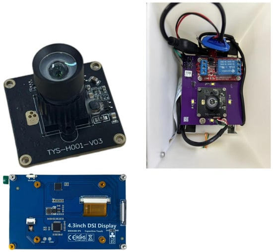
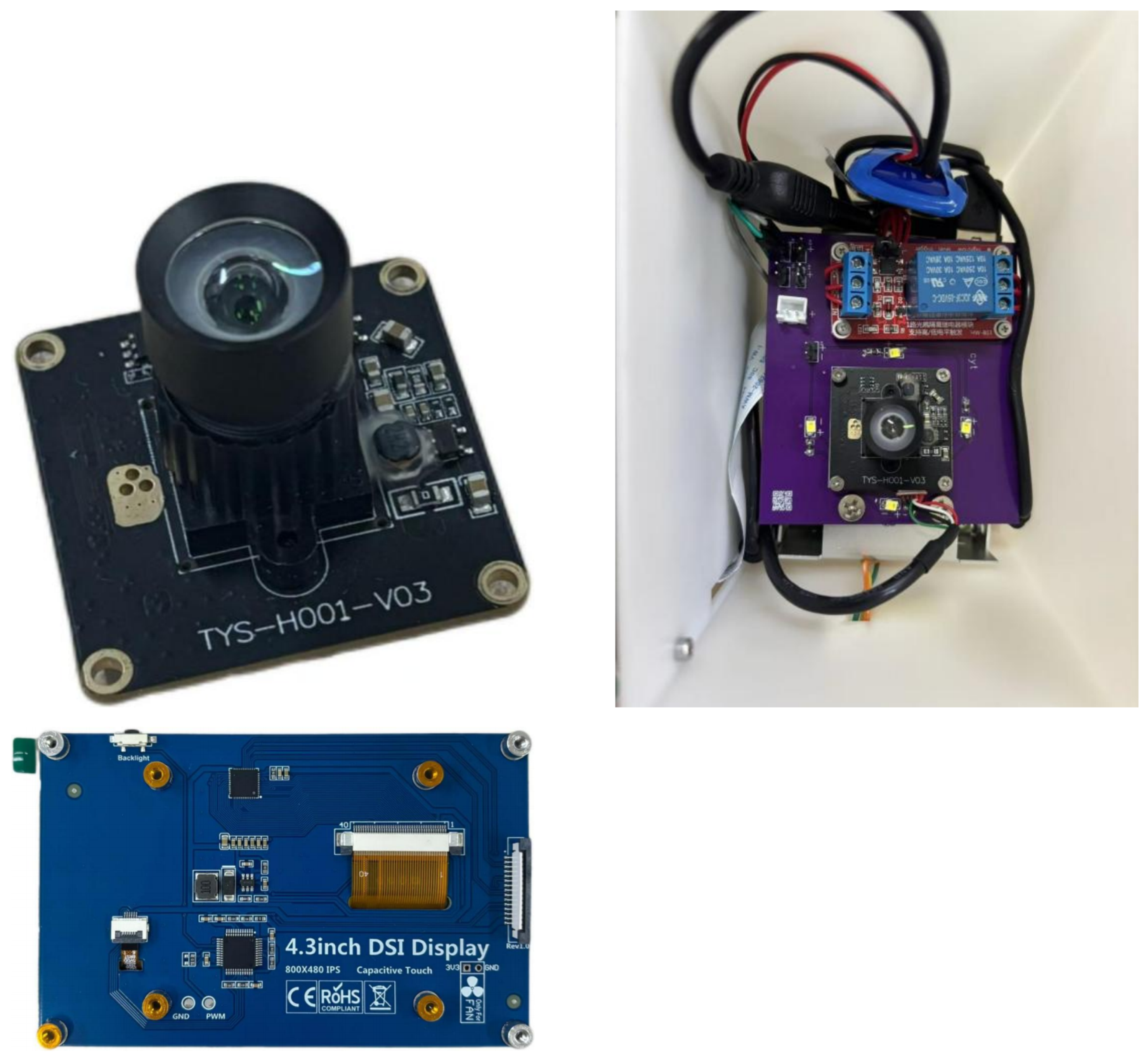
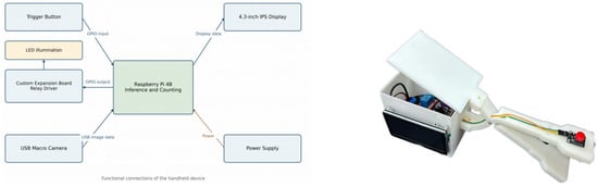
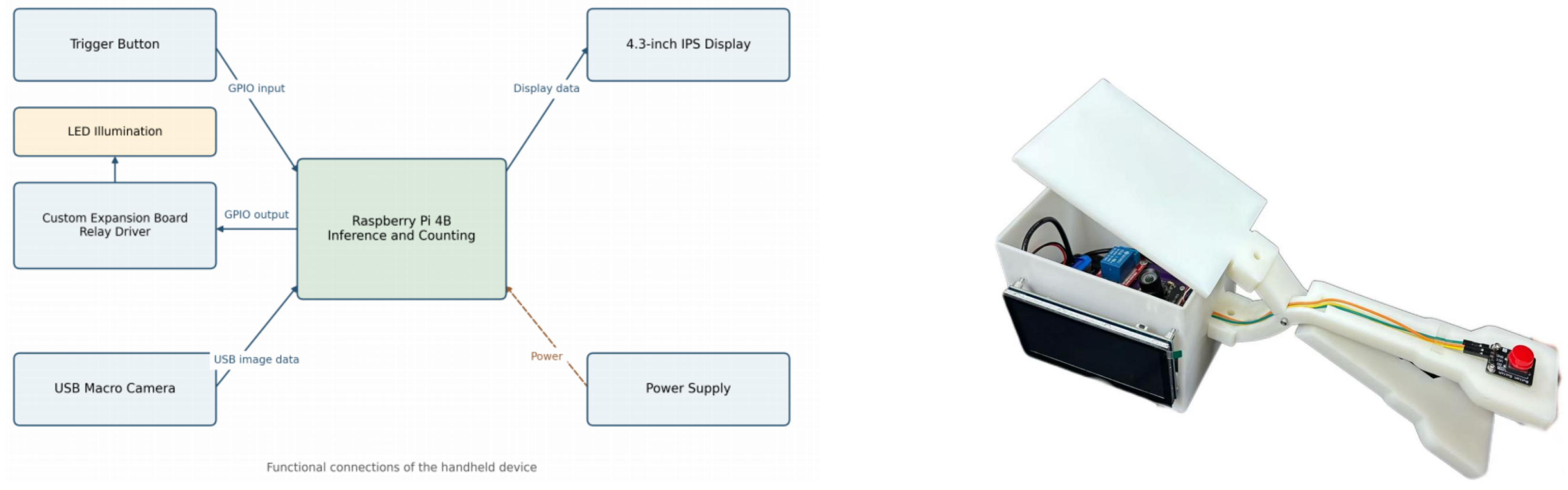
The prototype uses a Raspberry Pi 4B (Raspberry Pi Ltd, Cambridge, UK) with 2 GB RAM running Raspberry Pi OS (Bookworm, version 12), a TYS-H001-V03 5-megapixel USB macro camera, a 4.3-inch capacitive IPS display, a trigger, and four relay-controlled near-field LEDs (Figure 1 and Figure 2). The camera has a nominal 1/2.5-inch sensor with 2.2 μm pixels and MJPEG/YUY2 output. The camera and LEDs are mechanically coupled. The LED supply is 5 V and its reported maximum load is approximately 0.6–0.8 W; this is the illumination load, while whole-device power was measured separately with a USB power meter.

Figure 1. Prototype components: macro camera (upper left), internal integration (upper right), and display (bottom).

Figure 2. Functional connections (left) and the assembled handheld unit (right).

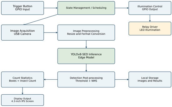
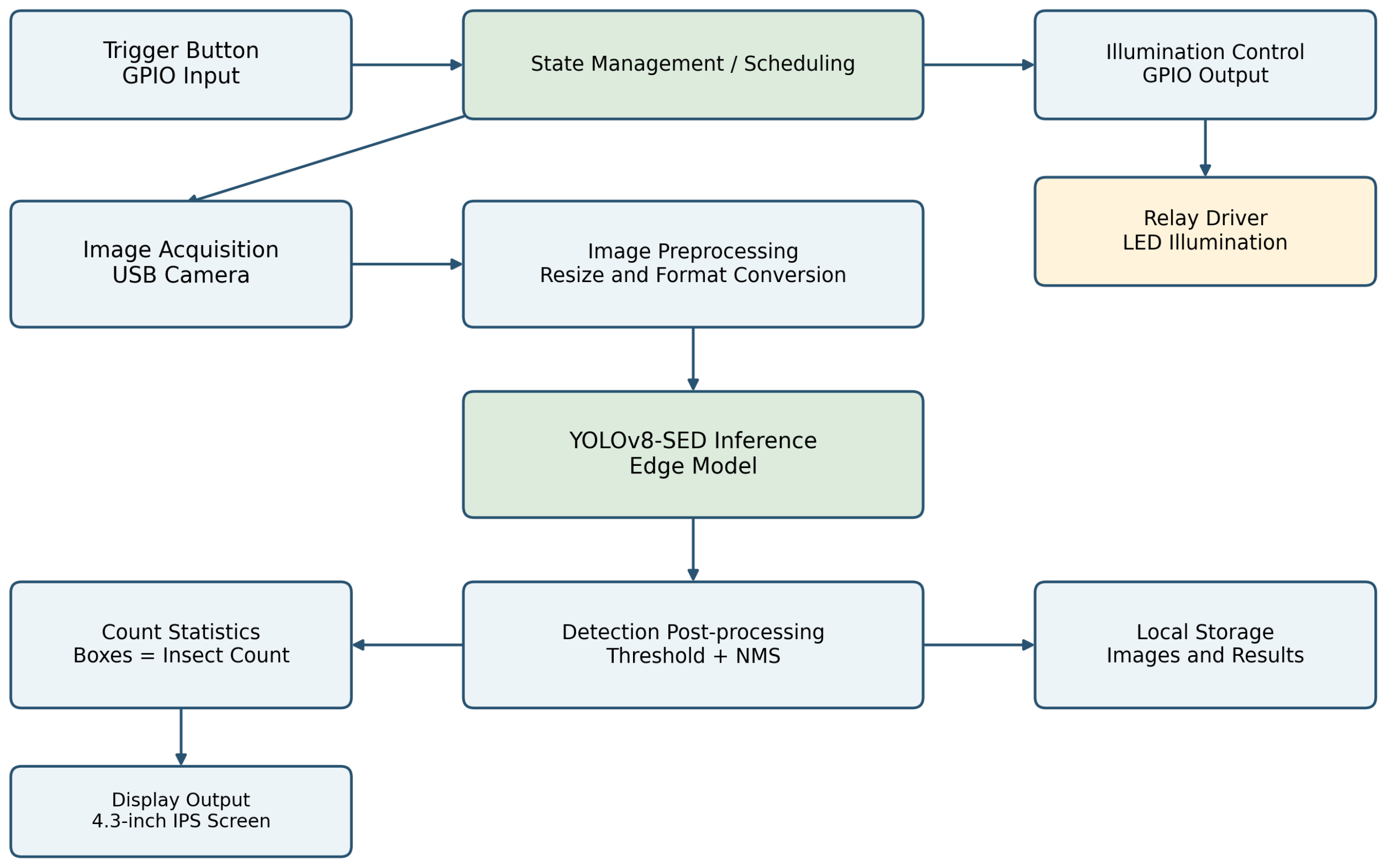
One trigger captures one image. Preprocessing resizes/formats the image to the actual $640\times 640$ detector input. The exported model runs locally on the Raspberry Pi CPU using ONNX Runtime 1.14.1 with FP32 precision. No INT8 or FP16 quantization was applied. Confidence filtering at 0.25 and non-maximum suppression (NMS) at IoU 0.70 precede counting, display, and local storage of the annotated result. The same reported thresholds were used for evaluation and field operation. The prototype does not require a network connection during inspection.

• Mechanical and Electrical Integration

The hardware was arranged for a short imaging distance. The handheld device comprised a Raspberry Pi 4B, expansion board, battery interface, display, camera, and LED sources. The trigger supplies the acquisition request, the expansion-board relay controls the illumination load, and the USB connection carries camera images to the processor. The display provides immediate feedback while local storage retains an observation record. The assembly photographs in Figure 1 show the documented camera, internal integration, and display components; these views are distinct from the performance measurements reported later.

The camera and LEDs were mounted together so that their relative positions remained fixed as the operator moved from leaf to leaf. This arrangement reduces changes in the position of the light source relative to the lens, although the actual distance and leaf angle still depend on how the device is held. Coupling the components mechanically does not constrain the leaf surface to a calibrated plane. The housing and handle support point-by-point operation rather than a fixed-area canopy scan. The operator must still position the lens, assess the focus, and present both surfaces.

The camera’s native resolution differs from the detector’s $640\times 640$ input. The camera-to-leaf distance during dataset and field imaging was approximately 5–12 cm, typically 6 cm. Using the nominal horizontal field angle of ${47}^{\circ }$, $W=2d\tan ({47}^{\circ }/2)$ gives an estimated horizontal coverage of 4.35, 5.22, and 10.44 cm at distances of 5, 6, and 12 cm. These are geometric estimates, not calibrated object-field measurements; focus, cropping, and resizing can change effective coverage. At 6 cm, a 3–3.5 mm object occupies approximately 5.7–6.7% of the estimated width.

The main housing measures approximately $118\times 84\times 117$ mm, excluding the handle. The handle is approximately 200 mm long, and the overall assembled length is approximately 318 mm. The battery is a single 18650 -format cell rated at 3.7 V and 3200 mAh (nominal energy 11.84 Wh). The typical active whole-device power is approximately 4.2 W, while the low-power operating condition is approximately 3.2 W. The ideal estimate $11.84/4.2=2.82$ h is comparable with the observed operating duration of approximately 2.7 h; this calculation does not measure usable battery energy or conversion efficiency. The approximate component cost was RMB 425.

2.2. Image Collection, Labels, and Partitions

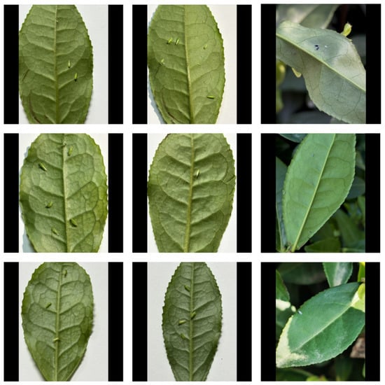
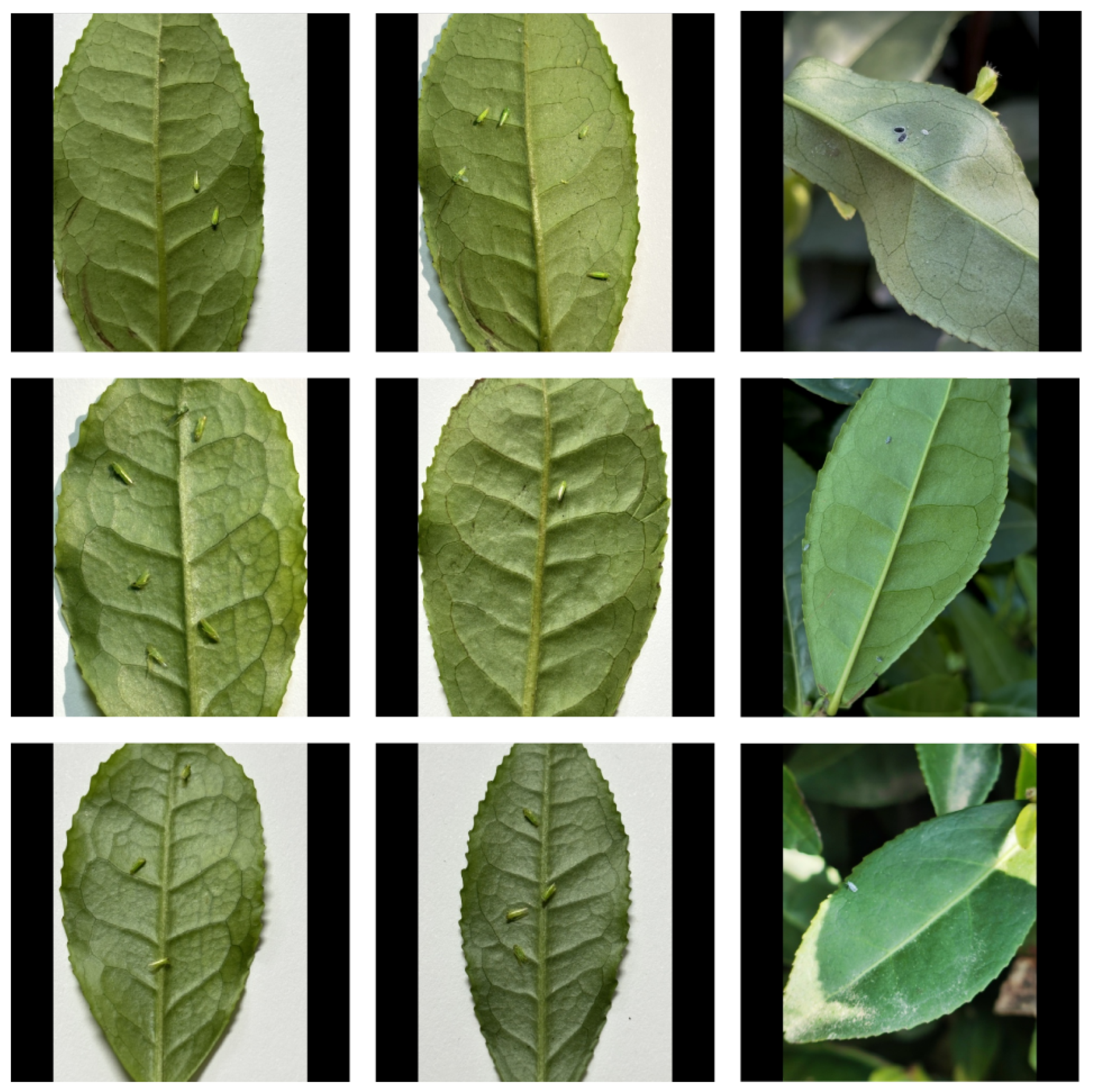
The dataset comprises 785 images collected during May–June and August–September 2024 at Yucha Village, Shaoxing, Zhejiang, China. Wild insects were photographed on intact tea shoots and on freshly detached leaves of cultivar Longjing 43; no laboratory colony was used. The material included buds, first–third young leaves, and mature leaves, with adaxial and abaxial views. Much of the close-up imaging used controlled laboratory illumination and plain backgrounds (Figure 3). Consequently, the internal test metrics predominantly characterize controlled imaging of field-collected material, not unrestricted natural-light field images.

Figure 3. Representative source images of tea small green leafhoppers on leaves.

Two annotators prepared adult and nymph bounding boxes using LabelImg (https://github.com/HumanSignal/labelImg, accessed on 30 October 2026), initially in PASCAL VOC XML and then normalized to YOLO format. A coauthor with an entomological background reviewed the annotations. Mean inter-annotator box IoU was 0.91. Targets with approximately two-thirds or more of the body hidden were excluded. Heavily occluded insects are outside the evaluated annotation scope.

The main dataset comprises 785 target-positive images: 326 adult-only, 289 nymph-only, and 170 mixed-stage images. Thus, 496 images contain adults and 459 contain nymphs; these overlapping counts must not be summed as mutually exclusive categories. The original split contains 628 training, 78 validation, and 79 test images, with 3371 target boxes in total. The test set contains 153 adult and 186 nymph instances. No field-pilot images were used to train the models.

The 785-image total excludes a separate set of 58 Aleurocanthus spiniferus images used only as auxiliary training negatives. These images are additional to the 785 target-positive images: the original training pool therefore contains 628 + 58 = 686 images, and the grouped training pool contains 630 + 58 = 688. None of the 58 occurs in validation or testing. They are not a third output class. All configurations use the same auxiliary negative set. The complete development collection contains 843 images (785 positive and 58 negative). An independent challenge set contains 42 Scirtothrips dorsalis images and 38 exuviae images outside those 843 images. It produced seven and four false detections, respectively: 0.167 and 0.105 false boxes/image, or 0.138 overall. These are false-box densities, not image-level false-positive proportions or proof of general non-target specificity.

A near-duplicate audit used perceptual-hash Hamming distance $\le 5$ and SSIM $\ge 0.95$. It identified 17 pairs: 12 within training, three within validation and two within testing. No cross-partition pair met these criteria. The pairs were retained to preserve the original dataset and split. Pair counts are reported without assuming that all pairs involve distinct images. Supplementary File S4 summarizes the reported partition and similarity-audit counts.

Two session-related analyses are distinguished. First, the 94.8% mAP@0.5 result was obtained by re-evaluating the original seed-42 YOLOv8-SED checkpoint on an adjusted 79-image test subset, without retraining. This checkpoint was fitted on the original 628 training images and selected by mAP@0.5 on the original 78 validation images. The adjusted allocation designated 626 images for training, 80 for validation, and 79 for testing; only the adjusted test subset was used in this analysis. Its designated training and validation partitions were not used for fitting or checkpoint selection. This diagnostic re-evaluation does not establish independence from the original training data and is not a session-grouped retraining result. Second, both YOLOv8n and YOLOv8-SED were retrained using five seeds on a separate session-grouped split containing 630 training, 77 validation, and 78 test images, shown in Table 1, grouping by acquisition date and garden block so that the same recorded session did not cross partitions. This second experiment selects checkpoints on its own validation set. Session grouping reduces a known dependence route but does not by itself establish independence across sites or all related plants.

Table 1. Target-positive images and annotated instances in the original and session-grouped partitions. The 58 auxiliary whitefly negatives are excluded from both 785-image totals, are used only in training and carry no target boxes.

Partition	Images	Adults	Nymphs	Total Instances
Training	628	1241	1472	2713
Validation	78	147	172	319
Test	79	153	186	339
Total	785	1541	1830	3371
Session-grouped retraining partition
Training	630	1235	1468	2703
Validation	77	152	179	331
Test	78	154	183	337
Total	785	1541	1830	3371

• Annotation Representation and Small-Target Distribution

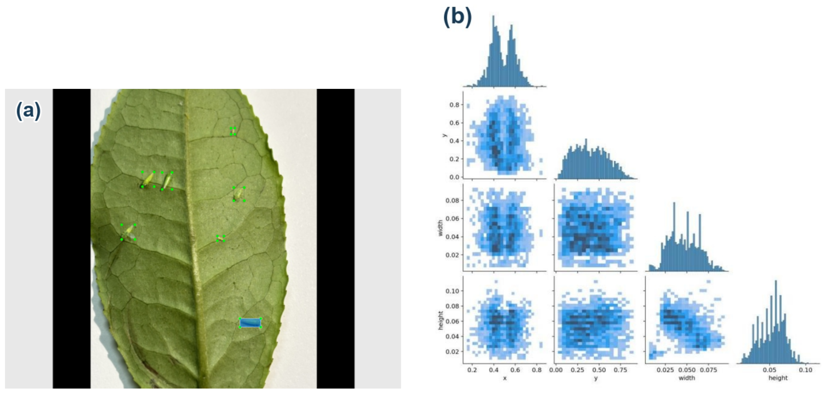
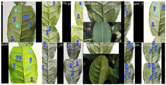
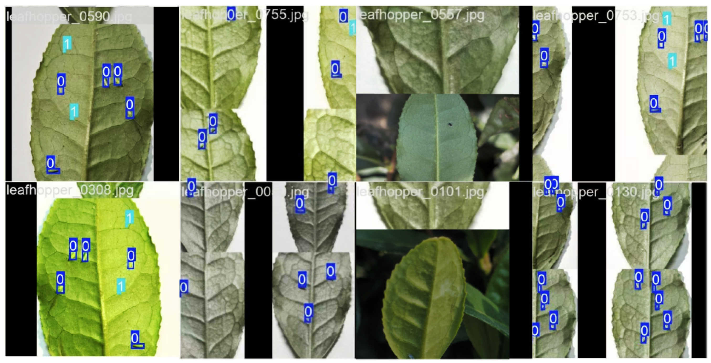
For an original image of width W and height H, a box was stored as its class index and normalized center and dimensions $(x_c/W,y_c/H,w/W,h/H)$. This representation permits annotation coordinates to be mapped to the resized input, but the apparent target scale still depends on how much of the original scene is included. The class mapping is fixed: 0 denotes adults and 1 denotes nymphs. Retaining that mapping during export is essential because a class-index swap would change the stage counts even if box locations were correct.

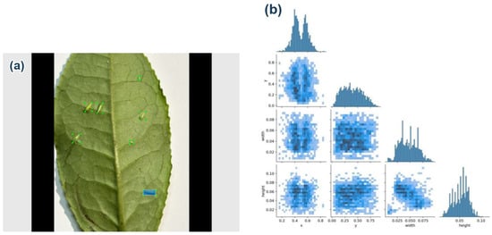
The label distribution reflects the way the images were collected. Target centers are concentrated in the leaf area, and box width tends to increase with box height. This is reasonable for a close-range camera aimed at one leaf, but it also limits what can be inferred about wide canopy images. The detector should therefore be viewed together with the acquisition protocol rather than as a general-purpose survey model. Most reported box widths occupy approximately 0.02–0.07 of the image width, and heights approximately 0.03–0.09 of the image height. At a 640-pixel input width, the former corresponds to about 13–45 pixels before feature-map reduction. Figure 4 shows annotation and label-distribution views.

Figure 4. Annotation examples and normalized label distributions. (a) Annotated example image; (b) normalized label distributions. Class 0 denotes adults and class 1 denotes nymphs.

Class balance also needs to be considered at the instance level. Nymphs account for 1830 of 3371 annotated targets (54.3%) and 186 of 339 test targets (54.9%). The adult/nymph proportions are therefore broadly similar in the original partitions, but this does not establish balance in leaf age, lighting, or insect pose. The instance totals show the amount of target material behind the aggregate scores; they do not establish independence among boxes from the same leaf or image. A single picture can contain several nearby insects with shared illumination and background.

2.3. YOLOv8-SED Architecture and Ablation Design

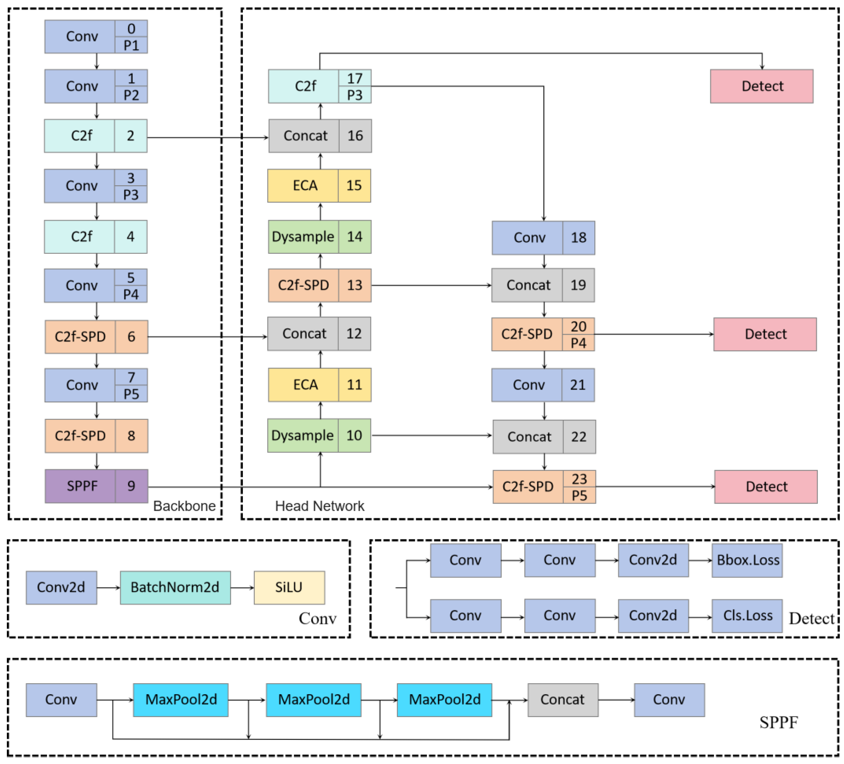
YOLOv8n is the baseline scale, consistent with the original 5.97 MB PyTorch (.pt) weight file and approximately 8.2 GFLOPs. The revised detector places C2f-SPD blocks in feature extraction, ECA at selected channel representations, and DySample in the feature-fusion upsampling path (Figure 5 and Figure 6). The operation-level details are given below so that the architecture overview and mechanism descriptions remain distinct. All eight single-, two-, and three-module combinations were evaluated under the same reported data split and training protocol. The ablation estimates configuration differences relative to YOLOv8n; it does not compare undocumented alternatives or establish that the modules act independently.

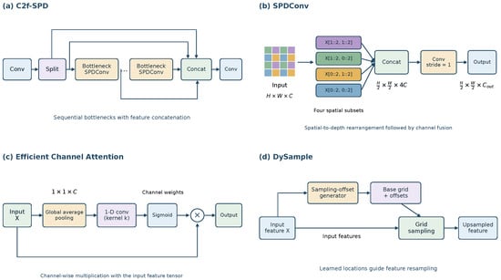
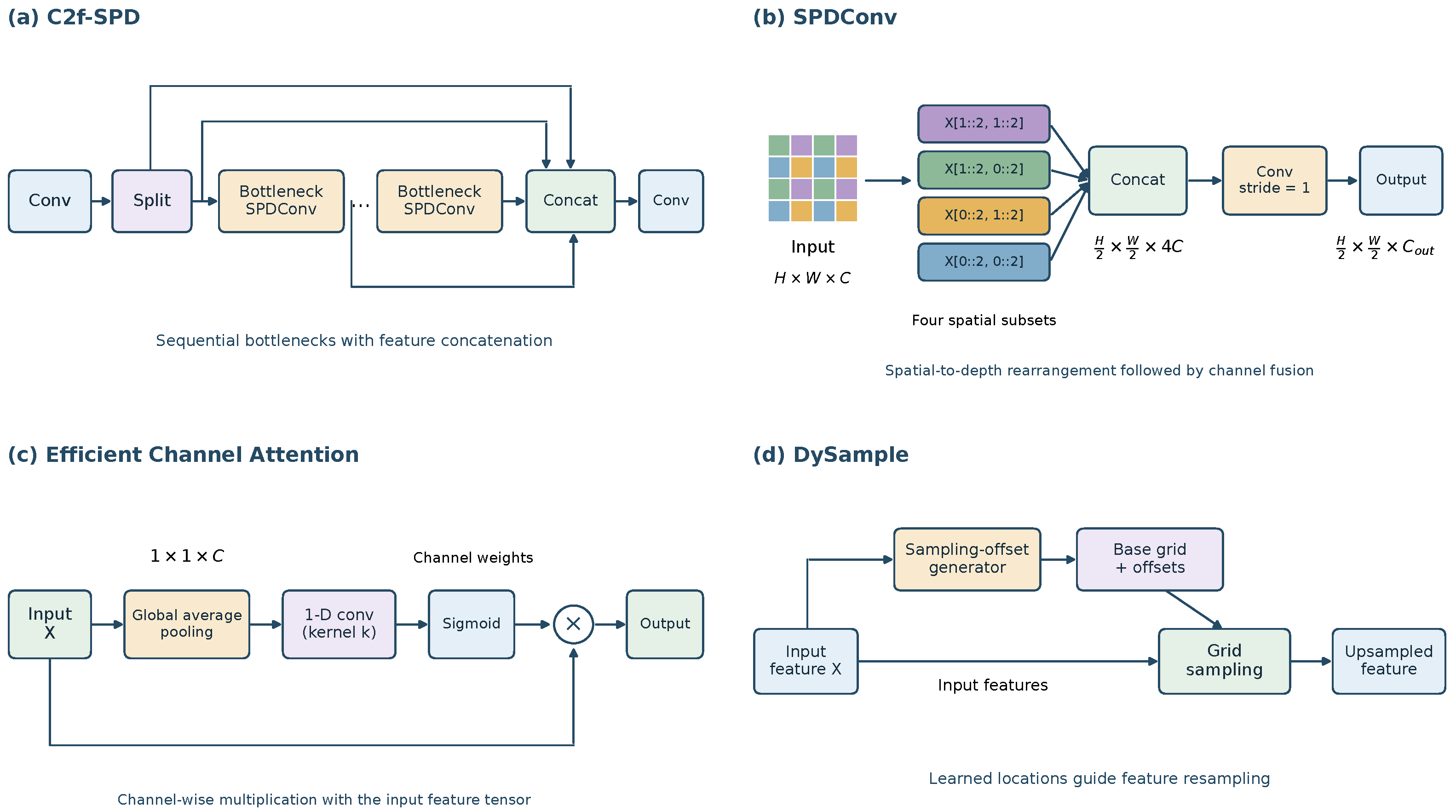
Figure 5. Operations incorporated into SED: C2f-SPD, spatial-to-depth, ECA, and DySample.

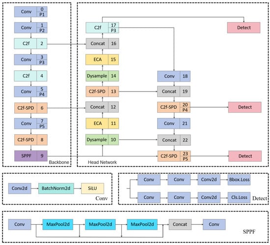
Figure 6. YOLOv8-SED connectivity. Supplementary File S5 separately identifies the available reconstruction and its layer-shape trace.

The eight configurations comprise the baseline, each single module, each pair, and the complete detector. Each was independently trained with five seeds using the same partitions and reported training settings. The main SED model and all main ablations use internal expansion $e=0.50$. A separate $e=0.55$ sensitivity variant is excluded from the main comparison. DySample is compared with nearest-neighbor upsampling; other upsampling families were not assessed.

2.3.1. Spatial-to-Depth Processing in C2f-SPD

The stride-two Conv layers 1, 3, 5, and 7 in Figure 6 retain the original backbone downsampling schedule. C2f-SPD changes the bottleneck processing inside selected C2f blocks rather than replacing those stride-two layers. Its purpose is to preserve local detail during feature processing after downsampling, when the already small insect representations are processed further. This distinguishes the backbone’s scale reduction from the subsequent feature transformation.

For scale factor 2, SPD rearranges the four spatial phases of each $2\times 2$ neighborhood into channels. Given an incoming feature tensor with dimensions $B\times c\times H\times W$, the rearranged tensor has dimensions $B\times 4c\times (H/2)\times (W/2)$ and contains the same number of values [14]. The four spatial positions remain available to the following $1\times 1$ convolution as channel information. This rearrangement–fusion design aims to reduce further degradation of local detail within the bottleneck. SPD itself involves no pooling or interpolation, but the learned projection is not generally invertible and cannot recover information discarded by earlier layers.

The bottleneck uses an encoding–fusion–restoration sequence: SPD, $1\times 1$ channel fusion, and depth-to-space (DTS). For its internal equal-width branch,

$$B\times c\times H\times W\stackrel{{\mathrm{SPD}}_2}{\to }B\times 4c\times \frac{H}{2}\times \frac{W}{2}\stackrel{1\times 1\mathrm{Conv}}{\to }B\times 4c\times \frac{H}{2}\times \frac{W}{2}\stackrel{{\mathrm{DTS}}_2}{\to }B\times c\times H\times W.$$

Here, c is the hidden branch width. The reduced spatial grid is intermediate: DTS restores $H\times W$ before the branch output is returned. Consequently, the neck C2f-SPD blocks at layers 13, 20, and 23 retain their respective incoming spatial resolutions. A residual connection, where enabled, additionally requires equal channel dimensions. The outer C2f projections determine the complete block’s input/output channels; spatial-size preservation does not imply identical external channel counts.

The intended efficiency mechanism combines parameter-free rearrangement, processing on the reduced spatial grid, and the hidden-channel configuration of the replacement bottleneck. For a convolution with kernel size k, groups g, and output grid $H_o\times W_o$, the convolutional weight count and multiply–accumulates (MACs), excluding bias and normalization, are

$$N_{\mathrm{weights}}={\displaystyle \frac{k^2{C}_{\mathrm{in}}{C}_{\mathrm{out}}}{g}}, \mathrm{MACs}=H_o{W}_o{\displaystyle \frac{k^2{C}_{\mathrm{in}}{C}_{\mathrm{out}}}{g}}.$$

For example, an equal-width path containing two dense $3\times 3$ convolutions has $18c^2$ convolution weights and $18HW{c}^2$ MACs. The $4c$-to-$4c$ projection in Table 2 has $16c^2$ convolution weights and $4HW{c}^2$ MACs. This comparison is restricted to the internal paths and excludes normalization, outer C2f projections, and repeat counts. In comparison with only one c-to-c $3\times 3$ convolution, the original weight count would instead be $9c^2$; therefore, a smaller kernel alone does not guarantee fewer parameters.

Table 2. C2f-SPD internal shape sequence: symbolic dimensions for the equal-width bottleneck branch.

Step	Tensor Dimensions $(\mathit{B},\mathit{C},\mathit{H},\mathit{W})$	Operation
Input	$(B,c,H,W)$	Hidden feature branch
SPD	$(B,4c,H/2,W/2)$	Spatial phases moved into channels
Channel fusion	$(B,4c,H/2,W/2)$	Learned $1\times 1$ projection
DTS	$(B,c,H,W)$	Spatial size restored

SPD and DTS have no learned convolutional weights. The fusion projection operates on one-quarter of the incoming spatial area, but its expanded channel counts must also enter the calculation. Thus, the comparison concerns the complete original and replacement bottlenecks, not a $1\times 1$ kernel in isolation. The measured whole-model results are 5.97 to 5.46 MB and 8.2 to 7.8 GFLOPs for baseline versus C2f-SPD alone, approximately 8.54% and 4.88% reductions from the rounded values. These measurements are not interpreted as universal per-block reduction ratios.

2.3.2. Efficient Channel Attention

ECA pools a feature tensor spatially to obtain a channel descriptor, uses a short one-dimensional convolution to model nearby channel interactions, applies a sigmoid, and multiplies the resulting weights back into the feature tensor [15]. The operation is economical because it avoids the fully connected bottleneck used by some channel-attention designs. The channel weighting can be summarized as

$$Y=\sigma \left(\mathrm{Conv}1{\mathrm{D}}_k\left(\mathrm{GAP}\left(X\right)\right)\right)\odot X.$$

The pooled descriptor summarizes the current feature channels; k is the channel-convolution kernel size; and ⊙ indicates multiplication, with the weights broadcast over spatial positions. This operation can change the contribution of channels sensitive to insect and background appearances without adding a dense channel-reduction network. It does not explicitly segment leaf veins or prove suppression of a particular confuser. Such an interpretation would require feature attribution or controlled background experiments, which were not performed here.

2.3.3. DySample Feature Reconstruction

DySample instead acts in the fusion path: it learns offsets for feature resampling, allowing upsampled positions to depend on input content [16]. A bilinearly resampled channel at a reference position can be expressed as

$$Y_c\left(q\right)=\sum _{p\in \mathcal{N}\left(u_q\right)}{X}_c\left(p\right)\prod _{d\in \{x,y\}}\max (0,1-|u_{q,d}-p_d\left|\right), u_q=q+\Delta q.$$

Here, q is expressed in input-feature coordinates, $\Delta q$ is a learned offset, and $\mathcal{N}\left(u_q\right)$ contains the neighboring grid positions used for interpolation. The module configuration specifies the offset groups and boundary handling for this sampling operation. Relative to fixed nearest-neighbor upsampling, the design permits the sampling locations to respond to local features. It may therefore help preserve the relation between a small target and the finer-resolution fusion grid, although this mechanism is a rationale rather than a directly measured boundary-recovery process.

2.3.4. Complete Architecture and Matched Combinations

The three operations address local feature rearrangement, channel weighting, and feature reconstruction. The main eight-configuration experiment keeps the original split, seeds, training settings, and operating thresholds fixed. The main SED internal expansion is $e=0.50$; the separate $e=0.55$ variant is not substituted into this comparison. Supplementary File S5 provides the model configuration (.yaml) and code for selected modules as Supplementary Materials.

2.4. Training, Checkpoint Selection, and Detection Metrics

Table 3 summarizes the training and inference. Training used an NVIDIA GeForce RTX 4080, with the recorded software environment PyTorch 1.11 and CUDA 11.3. The reported training and deployment environment is summarized with the confirmed settings in Supplementary File S5. The same experimental settings were applied across the eight YOLOv8-derived configurations.

Table 3. Reported training and deployment settings.

Setting	Value or Rule
Baseline/input	YOLOv8n/$640\times 640$ pixels
Maximum epochs/batch	100/16
Optimizer	SGD; initial learning rate: 0.01; momentum: 0.937; weight decay: 0.0005
Random seeds	12, 27, 42, 63, 89 for all eight configurations; original run: 42
Within-run checkpoint	Highest validation mAP@0.5; test metrics were not used to select weights
Architecture selection	Highest five-seed validation mAP@0.5; test results used only after selection
Pretrained initialization	COCO-pretrained YOLOv8n for YOLOv8-based configurations; transfer only shape-compatible tensors, with new/incompatible layers initialized separately
Learning-rate schedule	Initial learning rate 0.01; exact historical scheduler requires the original training arguments
Augmentation	Mosaic $p=1.0$; horizontal flip $p=0.5$; HSV gains $(0.015,0.7,0.4)$; brightness/contrast factors in $[0.75,1.25]$; MixUp $p=0.15$; custom CutMix $p=0.15$; default YOLOv8 scaling and translation
Confidence/NMS IoU	0.25/0.70 for the reported evaluation and deployment
Training platform	NVIDIA GeForce RTX 4080; reported PyTorch 1.11 and CUDA 11.3
Embedded platform	Raspberry Pi 4B CPU, 2 GB RAM, Raspberry Pi OS
Runtime/precision	ONNX Runtime 1.14.1/FP32; no quantization

MixUp and CutMix refer to the augmentation families, which are described in their original papers [18,19]. Mosaic was enabled with probability 1.0; horizontal flipping used probability 0.5; HSV gains were hgain = 0.015, sgain = 0.7, and vgain = 0.4; and random brightness and contrast factors were sampled over [0.75, 1.25]. MixUp and the custom CutMix module each used probability 0.15. Because CutMix is not exposed as a native operation in all Ultralytics YOLOv8 releases, we implemented it as an external augmentation module inserted after Mosaic. When triggered, it samples two images and their annotations, draws the mixing coefficient from Beta(1,1), composites the images, and updates the bounding-box annotations to the composed regions. RandAugment was not used.

For every run, the saved checkpoint with the highest validation mAP@0.5 was used for all final test metrics. This is not necessarily the last epoch, the epoch with maximum recall, or the checkpoint with maximum test performance. The original seed-42 values are retained separately for traceability. Five-run means and SDs describe variation due to training randomness on a fixed split; they are not a substitute for independent test sites or complete k-fold cross-validation. Full k-fold validation was not performed because of computational constraints.

• Repeated-Run Summaries and Checkpoint Separation

The main experiment comprises eight configurations and five seeds (40 runs). Architecture selection uses five-seed validation mAP@0.5, and within-run checkpoint selection uses the maximum validation mAP@0.5. Test evaluation follows these decisions. The original results.csv files and checkpoints were retained on the training server, providing a direct record of individual runs.

The repeated-run inventory comprises 40 original-partition ablation runs (Supplementary File S1), ten session-grouped runs (Supplementary File S2), and ten original-partition standard-comparator runs (Supplementary File S3). The requested 40+10 original-partition experiment is therefore separate from the additional grouped experiment. The supplementary compilation contains the reported aggregate summaries, the available historical seed-42 observations, and the complete run inventory; unavailable per-run entries in this compilation remain unfilled. Run-level F1 should be computed before averaging; five-run F1 summaries cannot be reconstructed by taking the harmonic mean of the reported mean precision and recall.

For metric z, the five-run mean and sample SD are $\overline{z}={\sum }_s{z}_s/5$ and $s_z={[{\sum }_s{(z_s-\overline{z})}^2/4]}^{1/2}$. F1 is calculated per run before aggregation. Seed variation on one split is distinct from replication across independent field sites.

Precision, recall, and F1 are defined using correctly classified, one-to-one matched detections:

$$P={\displaystyle \frac{TP}{TP+FP}}, R={\displaystyle \frac{TP}{TP+FN}}, F_1={\displaystyle \frac{2PR}{P+R}}.$$

(1)

A fixed-point detection match requires the correct class and IoU $\ge 0.5$, with one-to-one assignment. Unmatched predictions and annotations contribute to FP and FN. The NMS IoU of 0.70 controls within-image suppression and is distinct from the matching IoU. AP summarizes the precision–recall curve; mAP@0.5 averages class AP, and mAP@0.5:0.95 additionally averages ten IoU thresholds from 0.50 to 0.95 in steps of 0.05. Fixed-threshold precision/recall and the AP confidence sweep must be distinguished in the evaluation configuration in Supplementary File S5.

2.5. Pilot Field Protocol and Counting Units

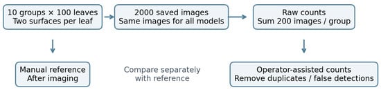
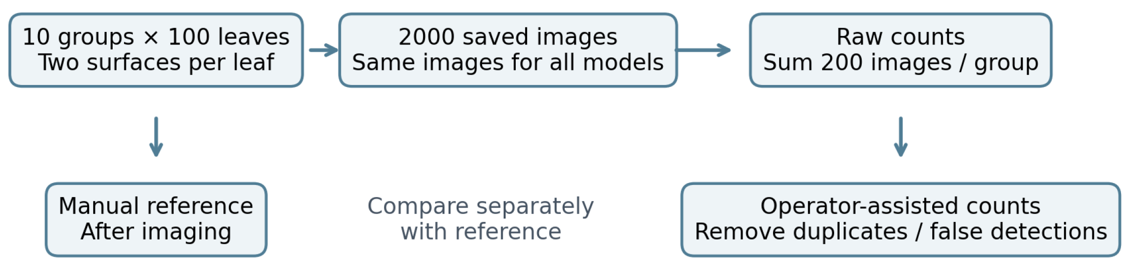
Field acquisition took place at Yucha Village, Shaoxing, Zhejiang, China (29.9350^° N, 120.7006^° E; approximately 65 m above sea level), using cultivar Longjing 43. The acquisition dates, recovered from the image records, span 12 May–3 June and 15 August–2 September 2024. Ten groups of 100 leaves were selected, giving 1000 leaves and 2000 images. Each leaf was photographed once from above (adaxial surface) and once from below (abaxial surface), without turning or touching the leaf during imaging. The same image collection was used for every detector comparison.

Imaging preceded manual inspection. The operator then gently turned the leaf and counted both surfaces, completing the leaf-level check within approximately 20 s of imaging. Two to three neighboring leaves were inspected when movement was noticed, but only individuals attributable to the sampled leaf were relevant to its reference count. This sequence reduces pre-imaging disturbance; it does not ensure that insects remain stationary between views or during subsequent inspection. The group reference is the sum for its 100 sampled leaves.

• Raw Automatic and Operator-Assisted Counts

For group i and model m, the raw count is the sum of all detections retained after confidence filtering and within-image NMS in its 200 images, before offline human review:

$$N_{m,i}^{\mathrm{raw}}={\displaystyle \sum _{j=1}^{200}}{\widehat{d}}_{m,i,j}, N_{m,i}^{\mathrm{assist}}=N_{m,i}^{\mathrm{raw}}-F_{m,i}-D_{m,i}.$$

(2)

Here, $F_{m,i}$ and $D_{m,i}$ denote mutually exclusive removals of obvious false detections and repeated appearances judged to represent the same insect. During review, paired leaf-surface images were compared using location, size, orientation, and visible appearance. Repeated appearances were counted once; clearly non-target detections, such as reflections, vein junctions, or dust, were rejected. No missed insects were added. NMS only suppresses overlapping predictions within an image and does not deduplicate insects between images.

The same trained observer acquired the images, made the manual reference counts, and subsequently reviewed the stored detections. Using the same observer allowed for a consistent operational rule for insect stage, marginal targets, and leaf identity. The model identities were concealed during separate reviews of each model’s outputs, but the observer knew the manual totals and used the original observation context to associate the records. Consequently, model blinding does not make the count reference and assisted output independent. Assisted counts are explicitly distinguished from automatic device output throughout the article. Group-level raw and assisted counts, net removals, and calculation details are provided in Supplementary File S6.

The four main field comparisons were run offline on the same 2000 saved images; they did not require four imaging passes. Review was repeated separately for each model. Supplementary File S6 presents the group-level counts, net removals, and error calculations for the four models.

For the image-annotation audit, two undergraduate annotators who had not participated in the field sampling, model development, or group counting independently annotated the 2000 saved field images using LabelImg and the training-data YOLO bounding-box convention. They were blinded to the model identities, reference group counts, and study hypotheses. A coauthor with an entomological background adjudicated disagreements. A true-positive match required the correct class and one-to-one IoU $\ge 0.5$. These annotation procedures are distinct from the unblinded observer’s assisted counting. Figure 7 summarizes the field acquisition and the separate raw automatic and operator-assisted counting paths.

Figure 7. Field acquisition and separate raw automatic and operator-assisted counting paths.

2.6. Count Agreement and Embedded Timing

For 100-leaf group i, the signed error is $d_i=N_{d,i}-N_{h,i}$, where $N_{h,i}$ is the direct manual count and $N_{d,i}$ denotes either raw or assisted output, analyzed separately. The descriptive summaries are

$$\mathrm{MAE}={\displaystyle \frac{1}{n}}\sum _i\left|d_i\right|, \mathrm{MRE}={\displaystyle \frac{100}{n}}\sum _i{\displaystyle \frac{|d_i|}{N_{h,i}}}, \mathrm{bias}=\overline{d}={\displaystyle \frac{1}{n}}\sum _i{d}_i.$$

(3)

All $N_{h,i}$ were positive; MRE would be undefined for a zero-reference group and such groups would require separate reporting. Pooled absolute relative error, $100{\sum }_i\left|d_i\right|/{\sum }_i{N}_{h,i}$, weights insects differently from the unit-mean MRE. The exploratory Bland–Altman limits of agreement are $\overline{d}\pm 1.96s_d$, using the sample SD of paired differences [20]. With only ten sampling groups, these limits are descriptive and their sampling uncertainty is substantial.

All timing tests on both platforms exclude the first three warm-up runs before calculating the effective-run statistics. Timing on the Raspberry Pi excludes those three warm-up runs and summarizes the five subsequent independent effective repetitions. GPU timing uses three warm-up runs followed by 30 effective runs; these GPU measurements are not the source of the reported embedded timing. Stage means and SDs and complete-cycle observations are reported separately. Total-cycle SD is computed from measured cycle totals, not by adding stage SDs. Leaf positioning, manual inspection, and offline review are outside the electronic timing interval. Active power is approximately 4.2 W; a separate five-measurement low-power record is $3.20\pm 0.21$ W (range 2.97–3.44 W).

3. Results

3.1. Five-Seed Ablation and Per-Class Performance

Table 4 presents the original-split results as mean ± SD over the five seeds. YOLOv8-SED reached $95.3\pm 0.7\%$ mAP@0.5 and $70.5\pm 1.0\%$ mAP@0.5:0.95, improvements of 6.5 and 9.2 percentage points over YOLOv8n. Recall increased by 10.5 points and F1 by 6.1 points. These are descriptive differences between means, not significance tests. All models share the same 79-image, 339-instance test set, so neither the images nor the five seeds constitute independent field replications.

Table 4. Eight configurations on the original test split: five-seed mean ± sample SD (%). Checkmarks indicate included modules. File size refers to the PyTorch checkpoint, not the FP32 ONNX model. GFLOPs and file sizes are configuration records rather than five-run statistics; the main SED expansion is $e=0.50$.

Model	C2f-SPD	ECA	DySample	P	R	F1	mAP@0.5	mAP@0.5:0.95	MB	GFLOPs
YOLOv8	×	×	×	$88.5\pm 0.8$	$87.2\pm 1.1$	$87.8\pm 0.9$	$88.8\pm 0.9$	$61.3\pm 1.1$	5.97	8.2
YOLOv8 + C2f-SPD	√	×	×	$87.8\pm 0.7$	$95.7\pm 1.0$	$91.6\pm 0.8$	$91.0\pm 0.9$	$65.5\pm 1.1$	5.46	7.8
YOLOv8 + ECA	×	√	×	$90.1\pm 0.6$	$88.4\pm 1.0$	$89.2\pm 0.8$	$93.9\pm 0.7$	$67.9\pm 1.0$	5.98	8.2
YOLOv8 + DySample	×	×	√	$88.7\pm 0.7$	$88.5\pm 0.8$	$88.6\pm 0.8$	$92.4\pm 0.8$	$66.6\pm 1.2$	5.99	8.2
YOLOv8 + C2f-SPD + ECA	√	√	×	$95.2\pm 0.6$	$87.6\pm 1.2$	$91.2\pm 0.9$	$94.5\pm 0.7$	$68.7\pm 1.0$	5.47	7.8
YOLOv8 + C2f-SPD + DySample	√	×	√	$89.4\pm 0.6$	$88.8\pm 1.0$	$89.1\pm 0.8$	$94.2\pm 0.7$	$68.3\pm 1.0$	5.48	7.8
YOLOv8 + ECA + DySample	×	√	√	$96.2\pm 0.5$	$87.3\pm 0.9$	$91.5\pm 0.7$	$94.9\pm 0.6$	$69.2\pm 0.9$	5.99	8.2
YOLOv8-SED	√	√	√	$90.3\pm 0.6$	$97.7\pm 0.8$	$93.9\pm 0.7$	$95.3\pm 0.7$	$70.5\pm 1.0$	5.99	8.2

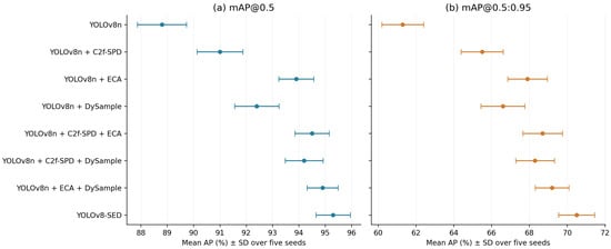
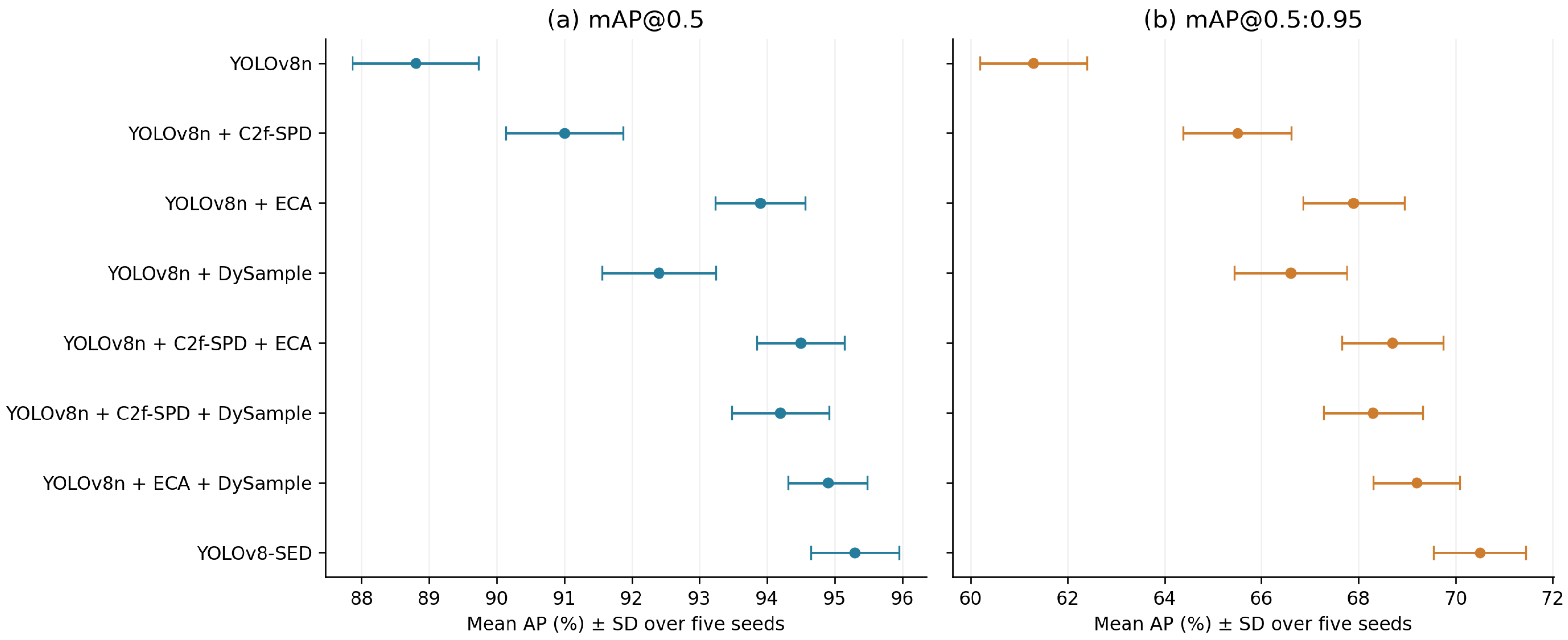
C2f-SPD alone increased mean recall by 8.5 percentage points while reducing mean precision by 0.7 points. ECA alone increased mAP@0.5 by 5.1 points, and DySample alone increased it by 3.6 points. The ECA–DySample pair had the highest precision ($96.2\pm 0.5\%$) but recall of only $87.3\pm 0.9\%$. Thus, maximizing precision alone does not maximize recovered insects. YOLOv8-SED gave the highest values for observed mean recall, F1, and both mAP measures. Differences of less than one point between some paired configurations are comparable with the observed run variation and should not be overinterpreted. Figure 8 labels each configuration explicitly.

Figure 8. Five-seed mean AP and one-SD error bars on the original partition.

The rechecked checkpoint-size records give 5.98 MB for ECA, 5.47 MB for SPD + ECA, and 5.48 MB for SPD + DySample; the latter two configurations have 7.8 GFLOPs. The standalone ECA and DySample additions change the baseline file size by approximately 0.01–0.02 MB, whereas C2f-SPD changes the bottleneck path. The main SED model remains $e=0.50$, 5.99 MB, and 8.2 GFLOPs. The $e=0.55$ variant is a separate sensitivity experiment, not the model behind these accuracy summaries. Weight tensors were stored in FP16 in the PyTorch checkpoints, while deployment used FP32 ONNX. Complexity follows the complete graph and its channel definitions and cannot be predicted by summing the rounded size changes of named modules. Raspberry Pi timing was measured for the baseline, SED, and standard comparators, not every ablation configuration.

• Descriptive Contribution of Module Combinations

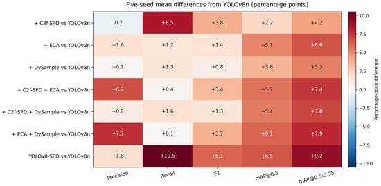
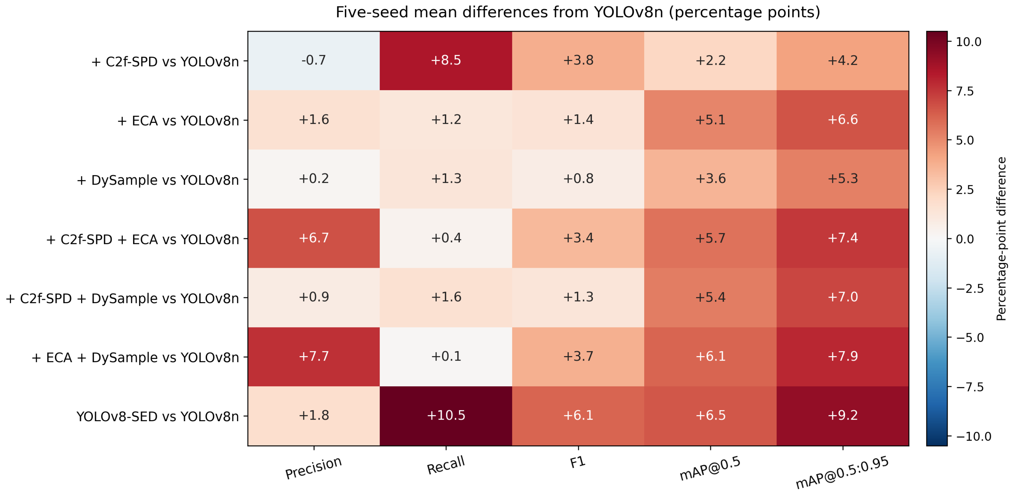
Figure 9 expands the ablation comparison to all five metrics using differences from the repeated-run baseline means. Single modules improve mean mAP@0.5:0.95 by 4.2 points for C2f-SPD, 6.6 for ECA, and 5.3 for DySample. The three two-module values are 68.7, 68.3, and 69.2%, respectively, and the complete configuration reaches 70.5%. This progression is consistent with a benefit in stricter localization, while the precision–recall tradeoffs show that all outcomes do not improve in parallel.

Figure 9. Metric differences from the YOLOv8n five-seed mean, in percentage points.

Adding the final module to each two-module combination increases mean mAP@0.5 by 0.8 points relative to SPD–ECA, 1.1 points relative to SPD–DySample, and 0.4 points relative to ECA–DySample. The corresponding mAP@0.5:0.95 increases are 1.8, 2.2, and 1.3 points. The precision, however, is lower than in the two combinations with the highest precision. These are configuration comparisons evaluated after validation-based selection, rather than independent causal estimates for individual modules.

These conditional differences are calculated from the rounded configuration means. They do not establish independent causal module effects, because the feature representations and optimization trajectories change when the configuration changes. The summaries also do not supply paired seed-level covariance for a confidence interval on a difference. The visible SD bars are therefore used to describe the scale of run variation rather than to assert a statistically significant rank among closely spaced configurations.

Adults had moderately higher metrics than nymphs (Table 5). Smaller nymph bodies provide a plausible explanation, although stage-specific illumination, occlusion, and appearance were not experimentally separated. Stricter-IoU AP remains considerably below AP@0.5, showing that accurate small-object boundary localization is still challenging even when an insect is detected.

Table 5. YOLOv8-SED per-class results on the original split, mean ± SD over five seeds (%). AP columns refer to one class; the corresponding two-class means are mAP.

Class	P	R	AP@0.5	AP@0.5:0.95
Adult	$91.2\pm 0.5$	$98.5\pm 0.7$	$96.2\pm 0.6$	$71.6\pm 0.8$
Nymph	$89.4\pm 0.7$	$96.9\pm 0.9$	$94.4\pm 0.7$	$69.4\pm 1.0$

The equal-class AP averages are $(96.2+94.4)/2=95.3\%$ and $(71.6+69.4)/2=70.5\%$, consistent with the full-model mAP means. Overall mAP SD cannot be obtained by averaging class SDs because the class scores within a run covary.

3.2. Original Single-Run Results, Split Sensitivity, and Training Behavior

Table 6 shows the historical seed-42 results separately from five-run summaries. The 98.3% recall belongs to the validation-mAP-selected checkpoint; it is neither the five-run mean nor a recall-based selection criterion. Re-evaluation of that fixed checkpoint on the adjusted 79-image subset gave 94.8% mAP@0.5, without retraining or selecting a new checkpoint. This is a diagnostic result for a modified test subset, not evidence of training/test independence. The five-seed grouped retraining described below is a different experiment.

Table 6. Historical seed-42 results from the original submission, retained separately from the five-seed summary. All values are percentages; checkmarks identify the included modules.

Model	C2f-SPD	ECA	DySample	P (%)	R (%)	mAP@0.5 (%)
YOLOv8	×	×	×	88.8	87.5	89.1
YOLOv8 + C2f-SPD	√	×	×	88.0	96.2	91.3
YOLOv8 + ECA	×	√	×	90.3	88.7	94.2
YOLOv8 + DySample	×	×	√	89.0	88.8	92.7
YOLOv8 + C2f-SPD + ECA	√	√	×	95.5	87.9	94.9
YOLOv8 + C2f-SPD + DySample	√	×	√	89.7	89.1	94.6
YOLOv8 + ECA + DySample	×	√	√	96.5	87.5	95.3
YOLOv8-SED	√	√	√	90.5	98.3	95.7

The validation comparison (Table 7) reports five-seed means on both partitions rather than comparing a validation mean with one seed’s test score. Consistent ranks are descriptive evidence of similar ordering; they do not establish the chronology of selection or eliminate dependence within the dataset.

Table 7. Validation and test mAP@0.5 (five-seed mean ± SD, %) on the original partition. Rank is identical for these two columns.

Configuration	Validation	Test	Rank
YOLOv8n	89.72±0.48	88.8±0.9	8
+ C2f-SPD	91.95 ± 0.42	91.0 ± 0.9	7
+ DySample	93.31 ± 0.39	92.4 ± 0.8	6
+ ECA	94.83 ± 0.45	93.9 ± 0.7	5
+ SPD + DySample	95.24 ± 0.37	94.2 ± 0.7	4
+ SPD + ECA	95.57 ± 0.41	94.5 ± 0.7	3
+ ECA + DySample	95.98 ± 0.36	94.9 ± 0.6	2
YOLOv8-SED	96.41 ± 0.33	95.3 ± 0.7	1

On the 630/77/78 session-grouped retraining split, baseline precision, recall, and mAP@0.5 are $83.60\pm 0.64\%$, $82.10\pm 0.72\%$, and $83.50\pm 0.59\%$. SED achieves $85.20\pm 0.56\%$, $92.70\pm 0.64\%$, and $90.10\pm 0.48\%$. The mAP advantage is 6.6 percentage points, compared with 6.5 points between the original-split five-seed means. Both models have lower absolute scores under grouping. These are descriptive paired-configuration differences; no significance test is inferred from the summary SDs. Grouped summaries and partition counts are listed in Supplementary Files S2 and S4.

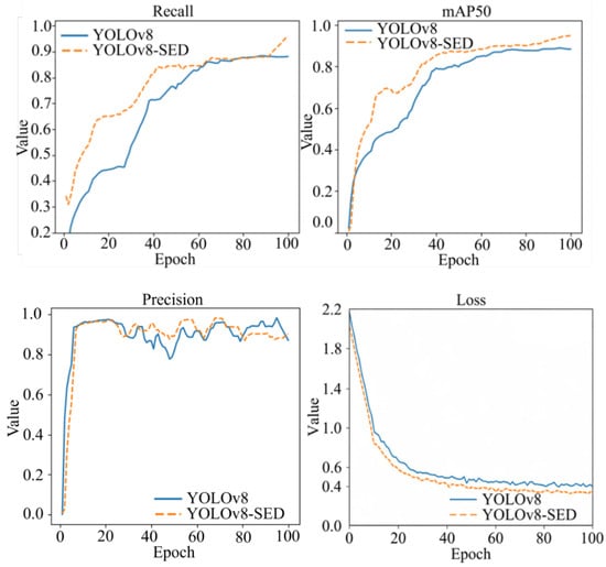
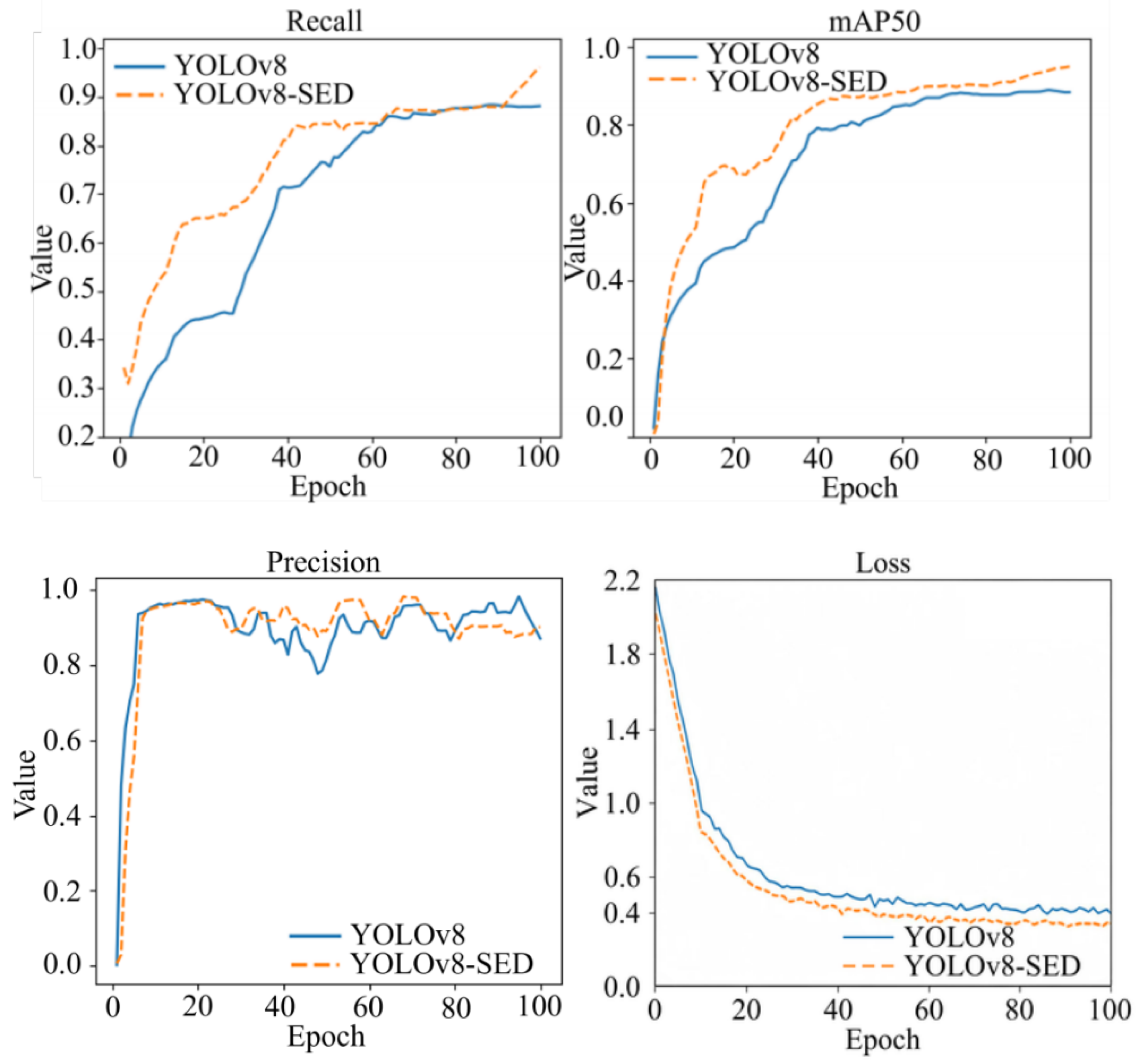
The maximum training duration was 100 epochs. The reported validation plots suggest an overall mAP plateau after approximately epoch 85; the author-reported inspection of the eight configurations also places broad stabilization near this point. However, the original YOLOv8-SED recall trace rises markedly during the final 5–10 epochs, from about 0.87 toward 0.95 (Figure 10). This cannot be described as complete stability of every metric. Small evaluation sets, changing confidence rankings, and checkpoint variation can contribute to such changes, but their individual effects cannot be determined from the available plot. The plot does not show a 0.983 validation-recall value and should not be used as evidence for that test statistic.

Figure 10. Single-run training and validation traces for baseline and SED. The seed-42 SED checkpoint was selected at epoch 92 by validation mAP@0.5.

Figure 10 shows precision, loss, validation recall, and mAP@0.5 traces. For the plotted seed-42 YOLOv8-SED run, the checkpoint with the highest validation mAP@0.5 was selected at epoch 92 and used for test evaluation. These curves describe the original single run and are not five-seed averages; convergence beyond the 100-epoch training limit was not tested. The late-epoch rise is reported rather than dismissed as proof of stable convergence. Figure 11 shows illustrative detections for adult (class 0) and nymph (class 1) leafhoppers.

Figure 11. Illustrative annotations and predictions for adult (class 0) and nymph (class 1) leafhoppers.

3.3. Embedded Execution and Survey Workload

The FP32 ONNX model completed one acquisition-to-display/save cycle in 1.34 s (SD 0.034 s) on the Raspberry Pi 4B across five independent repetitions. Table 8 reports the stage means and SDs; inference accounted for 69.4% of the mean cycle. The reciprocal rate is approximately 0.75 images/s, appropriate for deliberate still-image inspection rather than video-rate operation.

Table 8. Reported prototype stage times from five independent repetitions per stage (n = 5). Values are means and run-level SDs; the total row is the complete electronic cycle.

Stage	Mean (s)	Share (%)	SD (s)
Acquisition	0.21	15.7	0.008
Preprocessing	0.09	6.7	0.004
Inference	0.93	69.4	0.032
Display and storage	0.11	8.2	0.005
Total	1.34	100.0	0.034
Direct model comparison (same embedded protocol)
Model	Inference (s)	Full cycle (s)
YOLOv8n	0.91	1.32
YOLOv8-SED	0.93	1.34

Typical active power was approximately 4.2 W. The separate low-power record was $3.20\pm 0.21$ W, with a range of 2.97–3.44 W over five readings. It is not used as active power in the battery energy calculation.

The directly comparable baseline record is 0.91 s for inference and 1.32 s for the full cycle, versus 0.93 s and 1.34 s for SED. The main model therefore adds 0.02 s to both measurements; it does not provide a measured speed improvement. The first three warm-up runs were excluded on each platform. Supplementary File S8 summarizes the timing protocol and reported stage values.

For a complete 100-leaf group with two images per leaf, electronic cycles alone would take $200\times 1.34=268$ s (4.47 min). This is a calculated lower bound, not an observed survey duration. Leaf selection, positioning, focus adjustment, subsequent manual inspection, and offline review add unmeasured time. A timed complete survey, including operator work, was not conducted.

The software sequence is shown in Figure 12. A trigger starts LED illumination and camera acquisition, after which the obtained frame is passed to preprocessing and inference. The detector output is filtered and counted before the annotated frame and numeric summary are displayed and saved to local storage. The record includes the illumination status, image timestamp, and count for a single acquisition event. Keeping acquisition and output in the timing measurement avoids representing neural network execution alone as the time required to obtain a usable field record.

Figure 12. Embedded workflow from trigger and acquisition through inference, display, and local storage.

The complete stage mean is

$$T_{\mathrm{cycle}}=T_{\mathrm{acq}}+T_{\mathrm{pre}}+T_{\inf }+T_{\mathrm{out}}=0.21+0.09+0.93+0.11=1.34 \mathrm{s}.$$

The 0.41 s outside inference constitutes about 30.6% of the reported cycle. Even substantial acceleration of the network would leave these stages and the unmeasured operator work. This decomposition shows why model GFLOPs alone cannot establish practical survey speed: acquisition and output account for a material part of the measured electronic cycle, before any leaf handling or review.

3.4. Pilot Hundred-Leaf Count Comparison

Table 9 presents the four-model paired counts for ten 100-leaf groups. Manual reference counts range from four to nine insects per group, totaling 57. The raw totals for YOLOv8n, C2f-SPD, ECA, and SED are 54, 56, 57, and 60, respectively; the corresponding operator-assisted totals are 50, 51, 53, and 55. All assisted counts are less than or equal to the raw count for the same group and model, consistent with removal-only review.

Table 9. Paired field counts for ten 100-leaf groups. R: raw automatic sum over 200 images; A: operator-assisted count after offline review.

Group	Manual	YOLOv8n		+ C2f-SPD		+ ECA		YOLOv8-SED
		R	A	R	A	R	A	R	A
G01	5	5	5	5	5	6	5	6	5
G02	5	5	4	5	4	5	5	5	5
G03	7	6	6	7	6	6	6	7	6
G04	6	7	6	6	5	6	6	7	6
G05	4	3	3	4	4	5	4	4	4
G06	5	5	5	6	5	5	4	5	5
G07	9	8	7	9	8	9	8	9	8
G08	7	6	5	6	6	6	6	8	7
G09	4	4	4	4	4	4	4	4	4
G10	5	5	5	4	4	5	5	5	5
Total	57	54	50	56	51	57	53	60	55

Field acquisition: 12 May–3 June and 15 August–2 September 2024. Each group contains 100 leaves and 200 images. Group-level counts, net removals, and error calculations are provided in Supplementary File S6.

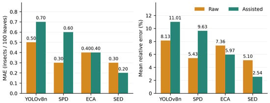
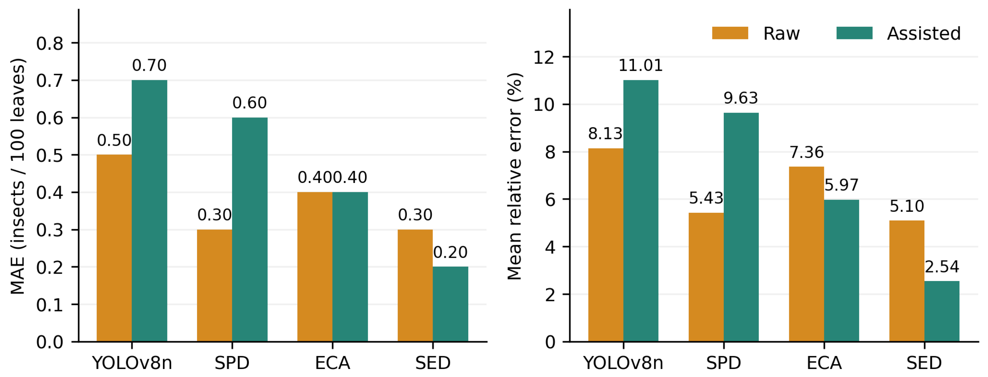
For SED, raw MAE is 0.30 insects per 100 leaves, MRE is 5.10%, and bias is $+0.30$ insects per 100 leaves (Table 10). Assisted MAE is 0.20, MRE is 2.54%, and bias is $-0.20$. Review reduces the SED total from 60 to 55, representing five net removals across G01, G03, G04, G07, and G08. These differences alone do not determine which removals were duplicates or false detections. The assisted total must not be equated with a true-positive total without matching the relevant image-level annotation records.

Table 10. Count-error statistics recalculated from Table 9. MRE is the mean of the ten group-specific absolute relative errors.

Model	Output	MAE a	MRE (%)	Bias a
YOLOv8n	Raw	0.50	8.13	−0.30
YOLOv8n	Assisted	0.70	11.01	−0.70
+ C2f-SPD	Raw	0.30	5.43	−0.10
+ C2f-SPD	Assisted	0.60	9.63	−0.60
+ ECA	Raw	0.40	7.36	0.00
+ ECA	Assisted	0.40	5.97	−0.40
YOLOv8-SED	Raw	0.30	5.10	+0.30
YOLOv8-SED	Assisted	0.20	2.54	−0.20

^a Units: insects per 100 leaves. Bias is model output minus manual reference. Each metric is calculated separately for raw and assisted outputs, using $n=10$ groups.

For the baseline and C2f-SPD models, removal-only review increases undercounting and MAE, because erroneous detections can partly offset missed insects in a total count. For ECA, absolute error is unchanged while MRE decreases because the distribution of group errors changes. The SED assisted values describe the combined detector–observer workflow, rather than autonomous counting accuracy. Group agreement is therefore interpreted together with the review procedure.

The exploratory SED Bland–Altman limits are approximately $-0.65$ to $1.25$ insects per 100 leaves for raw output and $-1.03$ to $0.63$ for assisted output, using bias $\pm 1.96$ sample SD of paired errors. These limits summarize ten observed groups and are not precise population limits.

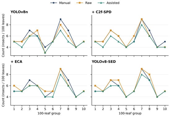
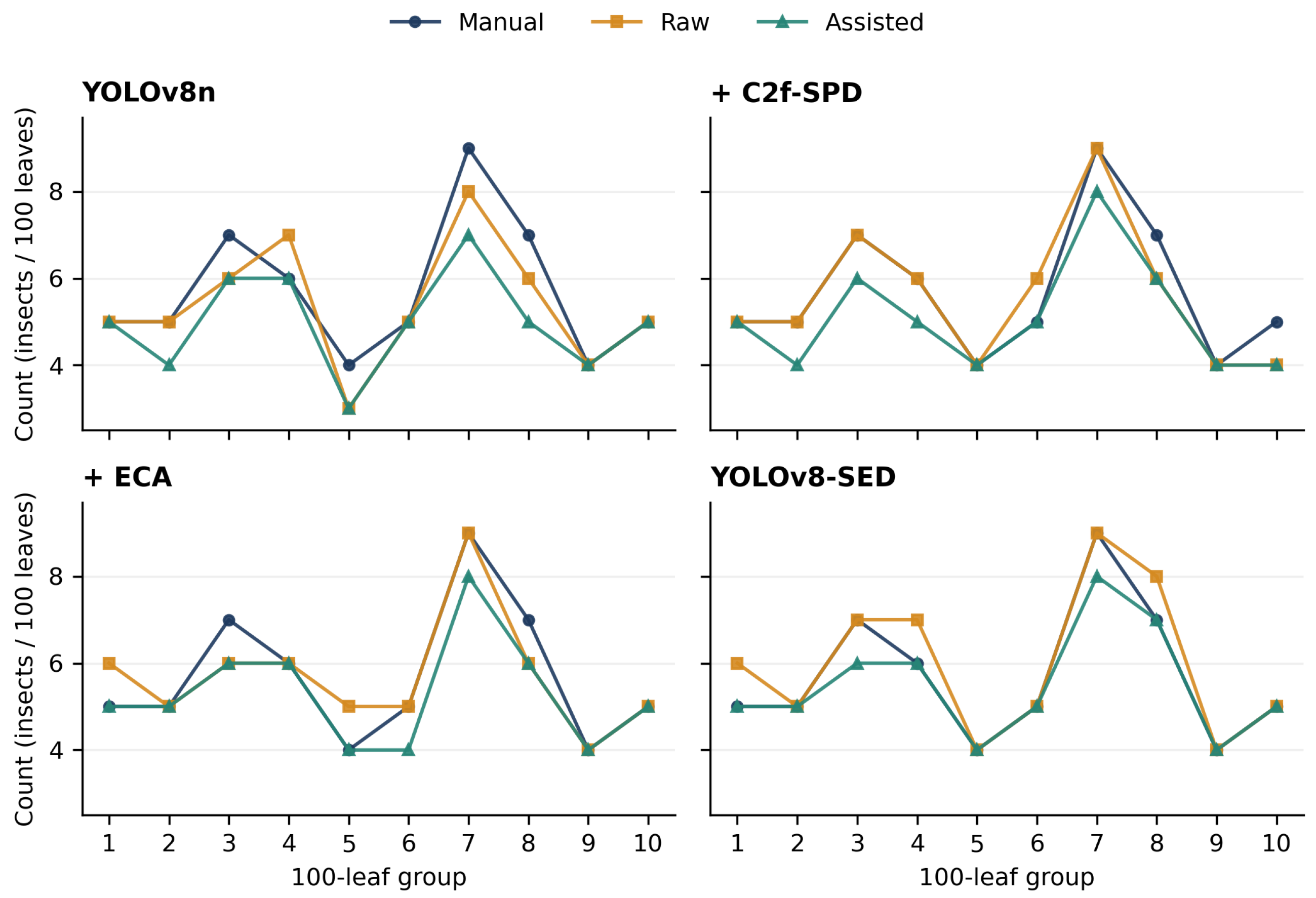
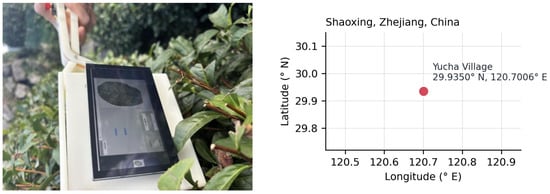
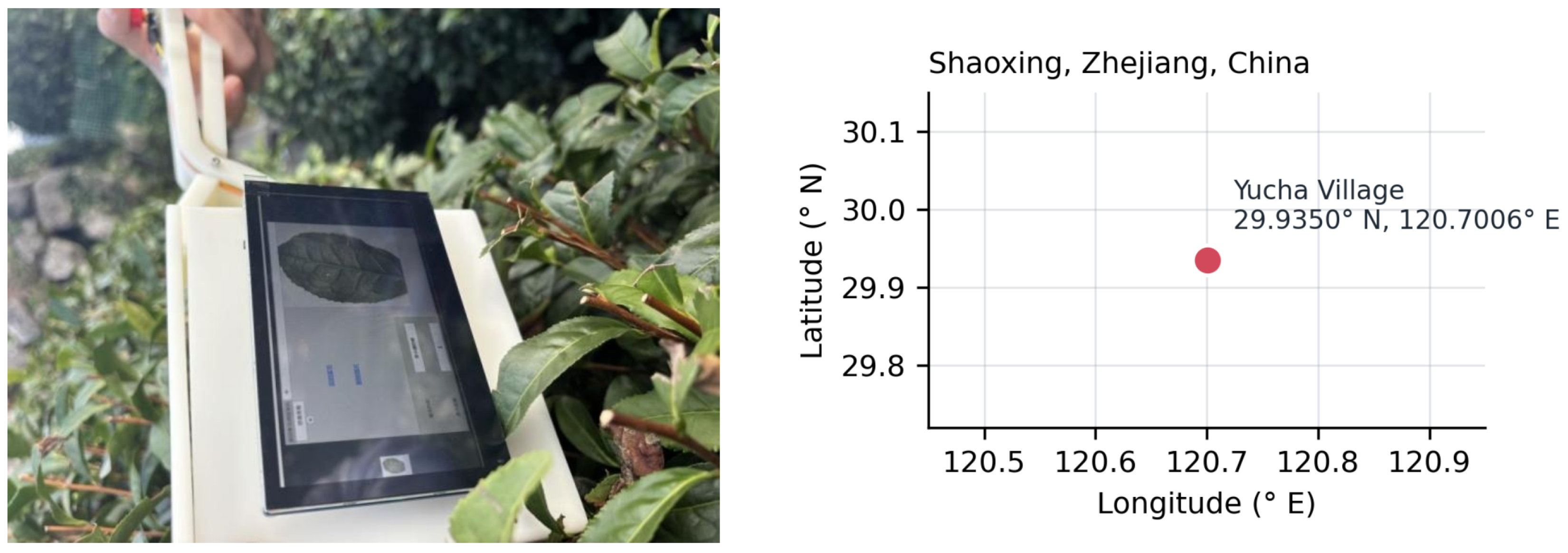
The annotated field examples identify non-target insects, leaf lesions, reflections, and dust as potential false-detection sources, and leaf-vein overlap, leaf hairs, and weak-light blur as missed-target sources. Supplementary File S7 gives the author-described inventory: four false-detection examples (one each involving an aphid, a leaf lesion, a reflection, and dust) and six missed-target examples (three vein-overlap, two leaf-hair occlusion and one weak-light blur). These selected cases are not used to infer the final field collection’s aggregate detection accuracy. Image appearances and unique insects are distinct counting units. Figure 13 compares the manual, raw automatic, and operator-assisted counts for each group and model. Figure 14 shows the raw and operator-assisted count errors (MAE and group-mean MRE), and Figure 15 shows the prototype in field use and the reported site coordinate at Yucha Village, Shaoxing.

Figure 13. Manual, raw automatic and operator-assisted counts for each 100-leaf group and model.

Figure 14. Raw and operator-assisted count errors: MAE (left) and group-mean MRE (right).

Figure 15. Prototype use (left) and the reported site coordinate at Yucha Village, Shaoxing (right).

3.5. Matched Lightweight Detector Comparison

The comparison uses standard YOLOv5n and YOLO11n configurations, each initialized from its own architecture’s official COCO-pretrained weights. The YOLOv8-derived ablations use YOLOv8n initialization with shape-compatible transfer; modified tensors are initialized separately. The models share the original split, training hyperparameters, augmentation settings, seeds, input size, and operating thresholds. The baseline and SED rows reuse the same five-run results and SDs as Table 4. Table 11 summarizes the comparison.

Table 11. Standard lightweight detector comparison. All accuracy values are five-seed mean ± SD (%). The .pt (MB) column reports the on-disk sizes of the original PyTorch checkpoint files; inference and cycle times were measured using their exported FP32 ONNX models on the Raspberry Pi. Checkpoint file size does not represent ONNX file size or runtime memory use.

Model	P	R	mAP50	mAP50–95	Params (M)	GFLOPs	.pt (MB)	Infer. (s)	Cycle (s)
YOLOv5n	$86.7\pm 0.9$	$85.4\pm 1.1$	$87.1\pm 0.9$	$59.2\pm 1.0$	1.86	5.6	3.72	0.72	1.12
YOLOv8n	$88.5\pm 0.8$	$87.2\pm 1.1$	$88.8\pm 0.9$	$61.3\pm 1.1$	3.01	8.2	5.97	0.91	1.32
YOLO11n	$89.7\pm 0.6$	$88.6\pm 0.8$	$90.5\pm 0.7$	$63.8\pm 0.8$	2.58	7.1	5.13	0.83	1.24
YOLOv8-SED	$90.3\pm 0.6$	$97.7\pm 0.8$	$95.3\pm 0.7$	$70.5\pm 1.0$	3.05	8.2	5.99	0.93	1.34

SED has the highest reported recall and mAP in this comparison, while YOLOv5n and YOLO11n have smaller files and shorter electronic cycles. The separate expansion-sensitivity variant ($e=0.55$) is excluded from the main comparison. Its reported size and timing summaries appear in Supplementary File S8; its seed, run count, and original evaluation records remain to be attached.

4. Discussion

4.1. Relation to Existing Tea-Pest Imaging Tasks

Damage recognition, direct detection, and trap monitoring observe different endpoints. RGB/hyperspectral methods can detect plant responses to feeding [9], direct insect detectors depend on current visibility, while traps additionally depend on attraction and exposure [10,11,12,13]. The present contribution is a close-range detector integrated with a handheld record-based inspection workflow. Published scores on different datasets cannot establish its superiority in hundred-leaf surveillance.

4.2. What the Model Comparisons Support

The five-seed results characterize optimization variation on the original split. The higher mAP@0.5:0.95 is consistent with improved localization, while precision and recall do not improve identically across configurations. The validation and test ranks agree, and the grouped retraining comparison retains a 6.6-point mAP advantage over the baseline. Absolute performance nevertheless falls under grouping. This supports further cross-session evaluation rather than a claim that all dependence or domain shift has been eliminated.

4.3. Operational Records and Workload

Local inference, display, and storage support inspection without a network connection. A useful record must also retain the leaf, surface, time, model version, and any human correction. The 1.34 s electronic cycle describes processing, whereas a complete survey also includes positioning, focus, direct inspection, and review. The calculated 4.47-min electronic lower bound for 100 leaves is not a measured survey duration.

4.4. Detection and Assisted Counting

Raw and assisted outputs answer different questions. Raw output measures accumulated image counts, whereas assisted output includes judgments about identity and non-target detections. Across the four models, review does not uniformly improve count error. Removing a false detection may expose a miss that it had offset numerically. The SED assisted result has the lowest observed group error, but the observer’s knowledge of reference counts can influence review decisions. The field results therefore support an operator-assisted inspection workflow.

4.5. Limitations and Further Validation

The principal test set contains 79 images; training-seed SDs describe optimization variability on a fixed split, not uncertainty across plantations. Session grouping separates recorded acquisition units, but the study still covers one site and cultivar. The 80-image negative challenge is small and taxonomically limited. The annotation rule excludes severely occluded targets, so performance on those targets requires separate evaluation.

Field counting comprises ten 100-leaf groups at low insect densities. The observer knew the manual counts during assisted review, and individual insects were not continuously tracked between views. Noncontact imaging reduces direct handling before capture but cannot exclude insect movement, duplicate appearances, or changes before reference inspection. The net reduction from raw to assisted totals does not alone distinguish duplicate removal from false-positive rejection. Field detection audits require explicit image identifiers, denominators, and matching rules before comparison with group counts.

The supplementary compilation documents confirm the settings, aggregate results, and available observations. Complete historical run records, source code, and weights remain necessary for exact reproduction; raw field images and labels are under controlled access. Checkpoint size is sensitive to serialization and precision; full-model complexity must be interpreted from its actual graph rather than inferred by adding rounded module-level file sizes. The expansion-sensitivity experiment is separate from the main $e=0.50$ model.

Further validation should use prospective sampling across sites and densities, blinded independent reference observers, traceable correction records, and representative field images. Complete survey time must include positioning, focus, manual inspection, and offline review. Calibrated field-of-view measurements and workload-controlled battery tests would improve the engineering evaluation. These requirements delimit the present feasibility study rather than demonstrating autonomous population monitoring.

5. Conclusions

YOLOv8-SED combines C2f-SPD, ECA, and DySample in a handheld Raspberry Pi prototype. The five-seed mAP@0.5 and mAP@0.5:0.95 on the original split were $95.3\pm 0.7\%$ and $70.5\pm 1.0\%$, exceeding the baseline means by 6.5 and 9.2 percentage points. Session-grouped retraining gave a mean mAP@0.5 of 90.1% for SED and 83.5% for the baseline. The main $e=0.50$ model uses a 5.99 MB PyTorch checkpoint and averages 1.34 s for the FP32 embedded capture-to-output cycle.

Ten groups of 100 leaves were evaluated, with raw automatic counts reported separately from operator-assisted outputs. The assisted counts followed offline duplicate and false-detection review by the same observer who knew the manual reference counts. The prototype demonstrates local detection and offline recording for close-range inspection. Broader prospective validation and complete survey-time measurements are needed to establish general field applicability.

References

- Qin, D.; Zhang, L.; Xiao, Q.; Dietrich, C.H.; Matsumura, M. Clarification of the Identity of the Tea Green Leafhopper Based on Morphological Comparison between Chinese and Japanese Specimens. PLoS ONE 2015, 10, e0139202. [Google Scholar] [CrossRef] [Scilit] [PubMed]
- Zhang, L.; Dietrich, C.H.; Xu, Y.; Yang, Z.; Chen, M.; Pham, H.T.; Le, C.C.V.; Qiao, L.; Matsumura, M.; Qin, D. Unraveling the hierarchical genetic structure of tea green leafhopper, Matsumurasca onukii, in East Asia based on SSRs and SNPs. Ecol. Evol. 2022, 12, e9377. [Google Scholar] [CrossRef] [Scilit] [PubMed]
- Shi, L.Q.; Zeng, Z.H.; Huang, H.S.; Zhou, Y.M.; Vasseur, L.; You, M.S. Identification of Empoasca onukii (Hemiptera: Cicadellidae) and Monitoring of its Populations in the Tea Plantations of South China. J. Econ. Entomol. 2015, 108, 1025–1033. [Google Scholar] [CrossRef] [Scilit] [PubMed]
- Ozawa, A. Sampling Method and Size Required for Estimation of Tea Green Leafhopper Empoasca onukii Matsuda Densities in Tea Fields. Chagyo Kenkyu Hokoku (Tea Res. J.) 2023, 136, 19–25. [Google Scholar] [CrossRef] [Scilit] [PubMed]
- Hunan Provincial Department of Agriculture and Rural Affairs. Tea Small Green Leafhopper Monitoring and Green Prevention and Control Technical Regulation; Technical Report HNZ184-2018; Hunan Provincial Department of Agriculture and Rural Affairs: Changsha, China, 2018.
- Kamilaris, A.; Prenafeta-Boldu, F.X. Deep learning in agriculture: A survey. Comput. Electron. Agric. 2018, 147, 70–90. [Google Scholar] [CrossRef] [Scilit]
- Redmon, J.; Divvala, S.; Girshick, R.; Farhadi, A. You only look once: Unified, real-time object detection. In Proceedings of the IEEE Conference on Computer Vision and Pattern Recognition; IEEE: New York, NY, USA, 2016; pp. 779–788. [Google Scholar] [CrossRef] [Scilit]
- Lin, T.Y.; Dollar, P.; Girshick, R.; He, K.; Hariharan, B.; Belongie, S. Feature pyramid networks for object detection. In Proceedings of the IEEE Conference on Computer Vision and Pattern Recognition; IEEE: New York, NY, USA, 2017; pp. 2117–2125. [Google Scholar] [CrossRef] [Scilit]
- Xu, Y.; Mao, Y.; Li, H.; Shen, J.; Xu, X.; Wang, S.; Zaman, S.; Ding, Z.; Wang, Y. A deep learning model based on RGB and hyperspectral images for efficiently detecting tea green leafhopper damage symptoms. Smart Agric. Technol. 2025, 10, 100817. [Google Scholar] [CrossRef] [Scilit]
- Li, Y.; Chen, T.; Xia, F.; Feng, H.; Ruan, Y.; Weng, X.; Weng, X. TTPRNet: A real-time and precise tea tree pest recognition model in complex tea garden environments. Agriculture 2024, 14, 1710. [Google Scholar] [CrossRef] [Scilit]
- Ye, R.; Gao, Q.; Qian, Y.; Sun, J.; Li, T. Improved YOLOv8 and SAHI model for the collaborative detection of small targets at the micro scale: A case study of pest detection in tea. Agronomy 2024, 14, 1034. [Google Scholar] [CrossRef] [Scilit]
- Wang, S.; Chen, D.; Xiang, J.; Zhang, C. A deep-learning-based detection method for small target tomato pests in insect traps. Agronomy 2024, 14, 2887. [Google Scholar] [CrossRef] [Scilit]
- Hakim, A.; Srivastava, A.K.; Hamza, A.; Owais, M.; Habib-ur-Rahman, M.; Qadri, S.; Qayyum, M.A.; Ahmad Khan, F.Z.; Mahmood, M.T.; Gaiser, T. YOLO-pest: An optimized YOLOv8x for detection of small insect pests using smart traps. Sci. Rep. 2025, 15, 14029. [Google Scholar] [CrossRef] [Scilit] [PubMed]
- Sunkara, R.; Luo, T. No More Strided Convolutions or Pooling: A New CNN Building Block for Low-Resolution Images and Small Objects. In Machine Learning and Knowledge Discovery in Databases; Springer: Cham, Switzerland, 2023. [Google Scholar] [CrossRef] [Scilit]
- Wang, Q.; Wu, B.; Zhu, P.; Li, P.; Zuo, W.; Hu, Q. ECA-Net: Efficient channel attention for deep convolutional neural networks. In Proceedings of the IEEE/CVF Conference on Computer Vision and Pattern Recognition; IEEE: New York, NY, USA, 2020. [Google Scholar] [CrossRef] [Scilit]
- Liu, W.; Lu, H.; Fu, H.; Cao, Z. Learning to Upsample by Learning to Sample. In Proceedings of the IEEE/CVF International Conference on Computer Vision; IEEE: New York, NY, USA, 2023. [Google Scholar] [CrossRef] [Scilit]
- Jocher, G.; Chaurasia, A.; Qiu, J. Ultralytics YOLOv8. Available online: https://github.com/ultralytics/ultralytics (accessed on 15 October 2026).
- Zhang, H.; Cisse, M.; Dauphin, Y.; Lopez-Paz, D. mixup: Beyond empirical risk minimization. In Proceedings of the International Conference on Learning Representations, Vancouver, BC, Canada, 30 April–3 May 2018. [Google Scholar]
- Yun, S.; Han, D.; Oh, S.J.; Chun, S.; Choe, J.; Yoo, Y. CutMix: Regularization strategy to train strong classifiers with localizable features. In Proceedings of the IEEE International Conference on Computer Vision; IEEE: New York, NY, USA, 2019. [Google Scholar] [CrossRef] [Scilit]
- Bland, J.M.; Altman, D.G. Statistical methods for assessing agreement between two methods of clinical measurement. Lancet 1986, 327, 307–310. [Google Scholar] [CrossRef] [Scilit]
Disclaimer/Publisher’s Note: The statements, opinions and data contained in all publications are solely those of the individual author(s) and contributor(s) and not of MDPI and/or the editor(s). MDPI and/or the editor(s) disclaim responsibility for any injury to people or property resulting from any ideas, methods, instructions or products referred to in the content. |
© 2026 by the authors. Licensee MDPI, Basel, Switzerland. This article is an open access article distributed under the terms and conditions of the Creative Commons Attribution (CC BY) license.