


Abstract
How to precisely depict the effects of high temperature on greenhouse crop growth and yield formation and derive optimal irrigation schedules remains an emerging challenge for current crop models. To address this issue, our study focused on drip-irrigated tomato plants grown in a greenhouse and adopted a two-factor experimental design with high temperature (TH: daily maximum temperature 35~40 °C) and two water levels (full irrigation, WH: 1.0Epan; deficit irrigation, WD: 0.6Epan), where Epan denotes the cumulative evaporation of a 20 cm standard evaporation pan. Forty-three parameters of the AquaCrop-OSPy model were screened using the Morris global sensitivity analysis method, and the selected highly sensitive parameters were processed via GLUE-based calibration and uncertainty characterization subjected to global optimization through a GLUE method to derive the model-based preferred strategy under high-temperature conditions in the greenhouse. On this basis, four indicators (yield, biomass (Bio), water consumption (ET) and water use efficiency (WUE)) were adopted to evaluate 20 combined scenarios of five temperature gradients and four irrigation strategies, which were then ranked using the TOPSIS–Entropy Weight (TEW) method. The results showed that the highly sensitive parameters of the AquaCrop-OSPy model under high-temperature greenhouse conditions included initial harvest index, water productivity, basal crop coefficient, maximum canopy cover, canopy growth coefficient, and days to maturity. After optimization using the GLUE method, the values of the above parameters were 70.9%, 15.2 g/m3, 1.36, 86.2%, 12.6%/d, and 108 d, respectively. The calibrated AquaCrop-OSPy model performed satisfactorily for canopy cover (CC), Bio, and yield under the evaluated experimental conditions, although ET and WUE simulations remained less accurate under combined high-temperature and deficit-irrigation conditions. The root mean square error of simulated CC was less than 7.2%, and the percentage errors of yield and Bio were less than 3.5% and 6.9%, respectively. Evaluation of the 20 temperature–irrigation coupled scenarios revealed that, among the scenarios evaluated, the 32~34 °C range combined with 1.1 or 0.9 Epan was associated with comparatively high simulated yield and WUE. Among the simulated scenarios evaluated using the TEW procedure, 34 °C + 1.1 Epan produced the highest comprehensive index (0.9283). The framework provides a model-based basis for identifying candidate irrigation strategies for greenhouse tomato under high-temperature conditions, which should be further tested experimentally.
1. Introduction
According to a 2024 report by the United Nations Educational, Scientific and Cultural Organization [1], approximately one-quarter of the global population is currently confronted with extremely high water scarcity stress. The frequent occurrence of extreme high-temperature events has further exacerbated the spatiotemporal imbalance of global water resource allocation and resulted in a significant reduction in global grain production, which serves as a critical stress factor constraining the sustainable development of agriculture. Reconciling the tension between water scarcity and food security has therefore become an urgent priority for countries worldwide. Protected agriculture, an essential production system for ensuring a stable vegetable supply, is equally threatened by high-temperature disasters, which pose new challenges to greenhouse environmental regulation and irrigation management. The semi-enclosed structural characteristic of greenhouses tends to cause the sustained accumulation of heat from solar radiation in the crop canopy and at the soil surface. When air temperature inside the greenhouse remains persistently above 35 °C, the structure of the D1 protein in the reaction center of photosystem II (PSII) is damaged and the carboxylation activity of ribulose-1,5-bisphosphate carboxylase/oxygenase (Rubisco) is inhibited, which in turn reduces carbon assimilation efficiency and substantially constrains crop yield formation [2,3]. Meanwhile, high-temperature conditions significantly increase the rate of crop water consumption and substantially intensify transpiration water demand, resulting in more complex dynamic patterns of crop water requirement [4]. Accordingly, how to precisely regulate the balance between crop water supply and demand under high-temperature greenhouse conditions and realize dynamic prediction of crop growth and development processes is a key scientific issue for ensuring the healthy and sustainable development of protected agriculture [5].
Previous studies have shown that regulating crop root-zone water dynamics is one of the most effective agronomic practices to alleviate the negative effects of heat stress [6]. Moderate irrigation can counteract heat-induced damage to the photosynthetic system to a certain extent, maintaining maximum leaf photochemical efficiency (Fv/Fm) and leaf area index (LAI) at appropriate levels. When the relative humidity inside the greenhouse is maintained at approximately 70%, crops can still maintain favorable stomatal conductance and leaf water potential under high-temperature stress [7]. A study on greenhouse cherry tomato by He et al. [8] further confirmed that net photosynthetic rate at the seedling stage decreased with rising temperature and increased with increasing irrigation volume. Specifically, under the treatment of high irrigation amount coupled with optimal temperature (125% Ep), the net photosynthetic rate reached 25.49 μmol/(m2·s), which was 48.8% higher than that under the combination of high temperature and low irrigation amount. Duan et al. [9] also observed in a study on heat injury in rice that irrigation can effectively mitigate heat damage to the photosynthetic apparatus by regulating the canopy micro-meteorological environment. However, current irrigation management for greenhouse crops still suffers from widespread practical issues, including excessively high irrigation quotas and inaccurate irrigation timing, which often cause a concurrent decline in both fruit yield and water use efficiency (WUE). Furthermore, excessive irrigation amount not only aggravates the ineffective consumption of water resources, but also triggers problems such as reduced soil aeration and secondary salinization, further restricting fruit yield formation and quality improvement [10].
Crop models serve as core mechanistic analytical platforms to reveal the feedback mechanisms among water, resource constraints, crop physiological responses, and grain yield output under climate change [11]. By quantitatively coupling environmental factors and crop physiological responses via mathematical equations, they provide technical tools for optimizing crop production management. At present, the widely used mainstream crop models include DSSAT, WOFOST, APSIM and AquaCrop. These models differ in research focus and underlying mechanisms, resulting in distinct application scopes. Nevertheless, it should be noted that systemic models such as DSSAT and APSIM impose high data requirements. Their applications rely on relatively complete meteorological, soil, agronomic, management and crop observational datasets. When measured field data are insufficient, calibrating cultivar genetic coefficients and evaluating model performance can be challenging, which restricts the practical application and extension of crop models in regions where field measurements are difficult to obtain. To address this issue, the Food and Agriculture Organization of the United Nations (FAO) developed the AquaCrop model in 2009. This model centers on the coupling relationship between water and yield. The most prominent advantage of this model lies in its parsimonious parameters and modest input data requirements. For instance, Ge et al. [12] compared the performance of AquaCrop and DSSAT under different mulching and irrigation schedules using greenhouse drip-irrigated tomato, and found that AquaCrop outperformed DSSAT in simulating canopy cover, with low relative errors for yield and WUE. Khafajeh et al. [13] verified the capability of the AquaCrop model to simulate ET, yield and Bio for greenhouse cucumber cultivation, offering decision support for irrigation management of greenhouse cucumbers. Furthermore, Locatelli et al. [14] assessed the long-term effects of deficit irrigation on greenhouse tomato yield using 30 year historical meteorological data, providing a basis for adaptive irrigation strategies under climate change.
The sources of error in the AquaCrop model are closely linked to the accuracy of parameter localization [15]. Traditional trial-and-error calibration relies heavily on the subjective empirical judgment of users, which makes it difficult to fully explore the parameter space and inter-parameter interactions. Where parameter compensation and equifinality may occur, the uniqueness and reliability of calibrated parameters cannot be guaranteed. Accordingly, effective management of model uncertainty is a critical component of improving crop model accuracy, and sensitivity analysis represents the core methodology for reducing model uncertainty and enhancing parameter calibration efficiency. Sensitivity analysis falls into two categories, local sensitivity analysis (LSA) and global sensitivity analysis (GSA). LSA only examines the gradient response of individual parameters near baseline values and neglects interactions among parameters, rendering it unsuitable for highly nonlinear crop growth models. GSA evaluates the contribution of parameters to output variance across their full value ranges, and is therefore more widely applied to sensitivity analysis of cultivar parameters in crop models. Within the GSA technical framework, the Morris method achieves preliminary dimensionality reduction of high-dimensional parameter spaces by calculating elementary effects of parameters. Its computational cost increases linearly with parameter dimensionality, making it appropriate for preliminary sensitivity screening of multi-parameter models [16]. The μ* statistic enables qualitative ranking of parameter importance, while σ indicates the presence of nonlinear or interaction effects, but it cannot quantitatively decompose the independent and interactive contributions of parameters to total output variance. By contrast, the Sobol’ method, grounded in variance decomposition theory, computes first-order and total-order sensitivity indices of parameters accurately via Monte Carlo sampling [17]. It can quantitatively resolve the contributions of parameter main effects and interaction effects to total output variance, but its computational cost scales as N × (2k + 2) with parameter dimensionality. Together, the two methods form a two-stage sensitivity analysis workflow of preliminary screening followed by refined calculation. Morris is first used to conduct preliminary screening and dimensionality reduction on 43 candidate parameters, and Sobol’ is then applied to perform variance decomposition on the reduced parameter set. This framework ensures quantitative accuracy while avoiding the Fourier spectrum leakage bias inherent to EFAST under high-dimensional parameter conditions [18].
Following the identification of key parameters, parameter calibration methods are required to achieve localized parameter calibration. Mainstream calibration approaches include the trial-and-error method, gradient descent-based methods (e.g., Levenberg–Marquardt), metaheuristic global optimization algorithms, and probabilistic–statistical methods. The trial-and-error method, essentially a univariate local adjustment strategy, is prone to falling into local optima under parameter coupling and equifinality [11]. Gradient descent-based methods are constrained by the highly non-convex nature of the AquaCrop objective function and tend to converge to spurious local minima. Metaheuristic algorithms can efficiently search for near-optimal solutions, but they only yield point estimates of parameters and fail to characterize the width of the posterior distribution or the equifinality phenomenon. The Generalized Likelihood Uncertainty Estimation (GLUE) method, proposed by Beven and Binley [17], screens behavioral parameter sets via Monte Carlo random sampling and likelihood functions. It enables parameter calibration, uncertainty interval characterization and equifinality handling, but lacks the capacity for quantitative analysis of parameter contributions [19].
These three methods play complementary roles. The Morris and Sobol’ methods are exclusively tasked with sensitivity quantification and are not involved in parameter optimization, together forming a sensitivity analysis chain of preliminary screening–refined quantification. GLUE independently undertakes parameter calibration and uncertainty analysis, performing Monte Carlo sampling and likelihood filtering on the key parameter set identified by Sobol’. The rationale behind this sequential coupling framework is as follows: Although the Morris + GLUE combination can accomplish calibration, the semi-quantitative screening from Morris cannot accurately characterize parameter interaction effects, and GLUE itself lacks the capacity for quantitative decomposition of variance contributions. Incorporating Sobol’ to conduct refined quantification prior to calibration enables the targeting of highly sensitive parameters while quantifying their main and interaction contributions, providing a quantitative basis for defining fixed versus floating parameter settings in GLUE. This framework ultimately forms a complete analytical pipeline of preliminary screening, refined quantification, calibration, and uncertainty characterization [20]. It should be emphasized that the calibration accuracy and uncertainty characterization performance of the GLUE method when integrated with the AquaCrop model under heat stress conditions remain to be validated.
To this end, our study takes greenhouse drip-irrigated tomato as the research subject. Based on two consecutive years of experiments with combined high-temperature and differential water treatments from 2024 to 2025, the Morris method is applied to screen 43 input parameters of the AquaCrop-OSPy model and identify sensitive parameters. Subsequently, the Sobol’ method is employed to perform refined variance decomposition on the screened parameters, quantitatively analyze the contributions of parameter main effects and interaction effects to the total output variance, and lock in the key parameter set. Finally, the GLUE method is adopted to implement Monte Carlo sampling and likelihood filtering on the identified key parameter set, so as to achieve parameter calibration and uncertainty interval characterization. The optimized model is then validated using data from an independent experimental year. Accordingly, the objectives of our study were (1) to clarify the differentiation patterns of AquaCrop-OSPy model parameter sensitivity across output variables under high-temperature greenhouse conditions and obtain a selected/calibrated parameter set; (2) to test the AquaCrop-OSPy model under high-temperature greenhouse conditions; (3) to evaluate irrigation strategies for greenhouse tomato under scenarios with different temperature and water combinations using the AquaCrop-OSPy model (the broader temperature × irrigation combinations are evaluated through model simulations, not experimentally tested treatments).
2. Materials and Methods
2.1. Experimental Site
The experiment was carried out from March to July in 2024 and 2025 at the Experimental Station for Efficient Agricultural Water Use in Henan Province (34°47′ N, 113°39′ E, altitude 80 m). The site has a warm temperate continental monsoon climate, with a long-term mean annual air temperature and precipitation of 14.2 °C and 548 mm, respectively. The experiments were conducted in two greenhouses with identical structure and dimensions. The steel frame greenhouses were oriented east–west, each covering an area of 84 m2 (8.0 m × 10.5 m). Vents were installed at the roof and on both the north and south sides. The greenhouse roof was covered with anti-drip polyethylene film, and 5 cm thick thermal insulation quilts were equipped to maintain interior air temperature during the seedling stage. The 0~60 cm soil layer inside the greenhouse was silty clay loam soil, with an average bulk density of 1.58 g/cm3 and an average field capacity of 0.30 cm3/cm3 (Table 1). The average soil pH, electrical conductivity and soil organic matter in the 0~20 cm soil layer were 6.4, 1.82 dS/m and 14.6 g/kg, respectively.
Table 1.
Soil types and hydraulic parameters in the 0–60 cm soil layer of the greenhouse.
2.2. Experimental Design
The local dominant tomato cultivar ‘Jingfan 404’ was selected as the experimental material. A wide–narrow row planting pattern was adopted, with wide and narrow rows of 65 cm and 45 cm. Seedlings were transplanted in March and harvested from late June to early July. Basal fertilizers applied were urea (46% N) at 112 kg/hm2, potassium sulphate (50% K2O) at 150 kg/hm2, and superphosphate (14% P2O5) at 120 kg/hm2. After the initiation of high-temperature and water treatments, topdressing was applied via a fertigation system along with irrigation water at the 2nd, 4th, 6th, 8th and 10th irrigation events. The topdressing rate was 188 kg/hm2 for urea and 25 kg/hm2 for potassium sulphate at each application. After the tomato fruit-setting stage, four fruit trusses were retained with four fruits per truss. Agronomic management practices (e.g., topping, pesticide spraying) were kept identical across all experimental plots.
The experiment was carried out in two greenhouses with identical structure (same dimensions, covering materials and ventilation configurations). A high-temperature treatment (TH) and two water gradients, i.e., high water (WH) and deficit water (WD), were established, with three replicates for each treatment. Each greenhouse contained three WH plots and three WD plots. Across the two greenhouse blocks, each water treatment had six plots. The experimental unit was the plot. The greenhouse was treated as a spatial block, and water treatment was treated as a fixed effect. The TH treatment was designed to maintain a daily maximum air temperature of no less than 35 °C and no greater than 40 °C, with temperature control primarily scheduled between 11:00 and 14:00. Air temperature inside the greenhouses was regulated by the BY-WSK smart greenhouse control system (Bangyou Hi-Tech Co., Ltd., Zhengzhou, China), which comprises a main control unit, distributed temperature-sensor modules, and an air-cooled compressor refrigeration device. Temperature sensors were installed at canopy height to collect real-time multi-point temperature data and transmit it to the main control unit. During the 11:00~14:00 period, whenever the temperature exceeded 40 °C, ventilation openings and internal fans were automatically activated for cooling, thereby maintaining temperature within the 35~40 °C range. Air temperature data were logged and updated automatically every 5 min. Both greenhouses were used under the same TH regulation, so ‘greenhouse’ was not treated as an experimental treatment but as a spatial block. Within each greenhouse, the two water levels (WH and WD) were randomized among plots with three replicated plots per treatment. In addition, temperature sensors and irrigation meters were installed independently in each plot, and the TH control was applied uniformly across the two greenhouses.
Irrigation frequency was scheduled according to the cumulative evaporation from a 20 cm standard evaporation pan (Epan), which was placed 30 cm above the crop canopy and adjusted upward as the plants grew. Daily evaporation from the preceding day was measured between 07:30 and 08:00 using a graduated cylinder with a precision of 0.1 mm. Irrigation events were triggered when cumulative evaporation reached 10 ± 2 mm. Two pan coefficients of 1.0 and 0.6 were adopted; here, 1.0Epan represents the well-watered condition, whereas 0.6Epan corresponds to the deficit-irrigated condition. It should be noted that temperature and water regulation treatments were initiated only after tomatoes entered the flowering and fruit-setting stages. Irrigation was performed using mulched drip irrigation. The emitter discharge rate of drip tapes was 1.1 L/h. A water meter with a precision of 0.001 m3 was installed at the inlet of each plot to quantify the water volume supplied to individual plots. In addition, a pressure gauge was fitted at the head of the main pipeline to regulate pipeline water pressure.
2.3. Measurements
2.3.1. Meteorological Factors
An automatic weather station at the greenhouse center continuously logged meteorological data, with all sensors positioned 2.0 m above the ground. Air temperature (Ta) and relative humidity (RH) were acquired by HOBO RS3-B and U23 Pro v2 data loggers (Onset Computer, Bourne, MA, USA). Solar radiation (Rs) came from an LI-200X pyranometer (Campbell Scientific, Inc., Logan, UT, USA), net radiation (Rn) from an NR-LITE2 net radiometer (Kipp & Zonen, Delft, The Netherlands), and wind speed from a WindSonic ultrasonic anemometer (Gill Instruments Ltd., Lymington, Hampshire, UK). All signals were sampled at 5 s intervals, 15 min averages were computed, and the final records were stored in a CR1000 data logger (Campbell Scientific, Inc., Logan, UT, USA).
2.3.2. Soil Water Content
For continuous monitoring of SWC during the crop growth period, an ECH2O system was used to monitor soil moisture. Data were automatically logged at 30 min intervals by a ZL6 data logger (Meter, Pullman, WA, USA). These sensors were installed at five depths (10, 20, 30, 40, and 60 cm) to capture the full soil profile.
2.3.3. Leaf Area Index and Canopy Cover
After transplanting, three plants of similar growth vigor were randomly selected and tagged in each plot. Plant height and leaf area were measured at seven-day intervals. Plant height was determined as the vertical distance from the stem base to the tallest apex using a measuring tape. For each tagged plant, the maximum transverse width and maximum longitudinal length of every leaf (starting from the cotyledons) were measured. Leaf area per plant was then estimated using the reduction-coefficient method, with a reduction coefficient of 0.684 determined from preliminary measurements. The leaf area index (LAI) was calculated as follows:
where L is the leaf length and W is the leaf width (cm); Sh is the row spacing (cm); and Sj is the plant spacing (cm). The canopy cover (CC) was estimated from LAI following the empirical exponential relationship based on the Beer–Lambert law adopted in the AquaCrop framework [21], expressed as follows:
2.3.4. Aboveground Biomass and Yield
At each growth stage, three representative plants were sampled and separated into stems, leaves, and fruits after root removal. Fresh weight was recorded for each fraction, which was then oven-dried. Samples were first oven-dried at 105 °C for 30 min for enzyme deactivation, followed by drying at 85 °C for 12 h. The dry matter of each fraction was weighed separately, and their sum represented the aboveground biomass. For yield assessment, twenty tomato plants were tagged in the center of each plot (three replicate plots per treatment), and total fruit weight per plot was recorded using an electronic balance (precision of 5 g).
2.3.5. Water Consumption
Water consumption (ET) was computed using the water balance approach:
where P is the precipitation (mm); Ir is the irrigation amount (mm); U is the groundwater recharge (mm); R is the surface runoff (mm); D is the deep percolation (mm); and ΔW is the change in soil water storage within the 0~60 cm layer (mm). In the greenhouse, precipitation was zero owing to the plastic film cover. The local water table remained below 5.0 m throughout the year, making groundwater recharge negligible. Moreover, surface runoff was considered negligible under mulched drip irrigation in the greenhouse. Deep percolation was assumed to be small based on the small individual irrigation amounts and the monitored soil water content in the 0~60 cm layer. However, this assumption is now explicitly acknowledged as a potential source of uncertainty in the water-balance estimate, especially because ET is one of the less accurately simulated variables. Therefore, the water balance equation includes only two terms: Ir and ΔW:
ET = P + Ir + U − R − D ± ΔW
ET = Ir+ΔW
Water use efficiency (WUE) and irrigation water use efficiency (IWUE) can be calculated using Equations (5) and (6), respectively:
where Y is the tomato yield (t/hm2). For comparison with outputs from AquaCrop, dry matter yield was substituted for grain yield in this study. Ir is the irrigation amount (mm).
2.4. AquaCrop-OSPy Model and Its Parameters
As a fundamentally water-driven crop model, AquaCrop partitions ET into soil evaporation (Es) and crop transpiration (Tr). It adopts canopy cover (CC) to characterize crop growth and development, while it computes final yield from biomass water productivity (WP) and harvest index (HI). The model comprises four integrated modules: meteorology, soil, crop, and management. To facilitate the coupling of parameter sensitivity analysis and parameter calibration procedures, our study employed the AquaCrop-OSPy model (version 3.0.12) for simulations. This variant shares the same underlying theoretical principle as the original AquaCrop model [22].
The AquaCrop-OSPy model adopts the canopy growth coefficient (CGC) to describe canopy development during the crop growth phase, as formulated in Equations (7) and (8). Canopy dynamics during the crop senescence phase are represented by the canopy decline coefficient (CDC), with its calculation formula given in Equation (9).
where CCt is the canopy cover at time t (%); CCx is the maximum canopy cover (%); CC0 is the initial canopy cover (%); t is the time (d); CGC is the canopy growth coefficient (%/d); and CDC is the canopy decline coefficient (%/d).
In the AquaCrop-OSPy model, ET, Es, and Tr are calculated by the following equations, respectively:
where CC* is the actual canopy cover (%); KcTr,x is the maximum transpiration coefficient; ET0 is the reference evapotranspiration (mm/d); Kex is the maximum evaporation coefficient; and Kr is the evaporation reduction coefficient.
ET = Es + Tr
Es = Kr × Kex × (1 − CC*) × ET0
Tr = KS,Tr × KS × CC* × KcTr,x × ET0
In the AquaCrop-OSPy model, the equations for calculating yield and Bio are as follows:
where Bio is the aboveground biomass (t/hm2); WP is the normalized water productivity (g/m2); Y is the yield (t/hm2); fHI is the harvest index adjustment factor; HI0 is the reference harvest index.
Y = fHI × HI0 × Bio
2.5. Morris Global Sensitivity Analysis
Global sensitivity analysis was conducted using the Morris method to identify parameters with significant influences on model simulation under high-temperature conditions. This method adopts a one-factor-at-a-time (OAT) trajectory design and performs random sampling in a multi-dimensional parameter space. Each trajectory comprises k + 1 sampling points, and at each point only one parameter value is changed by a fixed step size Δ while all other parameters remain unchanged. The elementary effect (EE) of each parameter is formulated as
After multiple trajectory samplings, the mean absolute elementary effect (μ*) and the standard deviation (σ) are computed statistically for each parameter.
where r is the number of trajectories. The classification of parameter sensitivity was based on a relative threshold approach, as shown in Table 2 and Table 3. A total of 43 crop parameters were selected, and their sensitivity with respect to yield, Bio, and CC was analyzed. The number of trajectories was set to three times the number of parameters (132 trajectories), yielding a total of 5808 simulations.
Table 2.
Parameters and value ranges of AquaCrop-OSPy model for greenhouse tomato.
Table 3.
Classification criteria by relative threshold method.
2.6. Sobol’ Variance Decomposition and GLUE-Based Parameter Calibration
After screening highly sensitive parameters with the Morris method, a two-stage approach combining Sobol’ variance decomposition and GLUE was adopted for parameter calibration and uncertainty analysis. In the first stage, variance decomposition was performed on the screened parameter set using the Sobol’ method, to quantitatively decompose the contributions of individual (first-order) effects and interaction effects of each parameter to the total output variance. In the second stage, the GLUE method was applied to the identified key parameter set to implement Monte Carlo sampling and likelihood filtering, completing parameter calibration and characterization of uncertainty intervals.
The first stage covers Sobol’ variance decomposition and optimal parameter identification. First, the first-order sensitivity index (Si) and total-order sensitivity index (STi) of each parameter are calculated. The proportional contributions of individual parameters and their interaction effects with other parameters to the total output variance are then quantified.
where Si is the first-order sensitivity index, representing the contribution proportion of the individual parameter Xi varying independently to the total output variance; Xi is the i th input parameter; VXi denotes the variance taken over Xi; Y is the model output response variable; V(Y) is the total output variance; is the conditional expectation with Xi fixed at a given value; STi is the total order sensitivity index, which includes the main effect of parameter Xi as well as the total contribution of its interactions with all other parameters.
The second stage is GLUE parameter calibration. Reasonable variation ranges are defined for each parameter based on prior knowledge. High-contribution parameters identified by Sobol’ (HI0, WP, CCx) were assigned wider ranges; moderate-contribution parameters (Kcb, CGC_CD) were assigned intermediate ranges; and the low-contribution parameter (MaturityCD) was assigned a narrower range. A total of 10,000 parameter combinations are generated through extensive Monte Carlo random sampling in the parameter space. Each parameter set is input into the AquaCrop-OSPy model for simulation, and the goodness of fit between simulated results and measured data is evaluated via the likelihood function. Parameter sets with values above the behavioral threshold are retained as behavioral parameter sets, to achieve parameter calibration and characterization of uncertainty intervals. The likelihood function is defined as
where yobs,i is the i th observed value; ysim,i(θ) is the simulated value; is the observation error variance. A higher likelihood value indicates better model simulation performance under the corresponding parameter set.
In our study, Morris was used only for preliminary screening and dimensionality reduction; Sobol’ was used only for variance decomposition and quantification of main and interaction effects; GLUE was used only for calibration and uncertainty characterization. Sobol’ was not used to calibrate parameters, and GLUE was not used to decompose variance. The sequential framework was intended to avoid blind calibration and to provide a quantitative basis for fixing or floating parameters in GLUE.
2.7. Model Evaluation
The data processed by THWH in 2024 was used for calibration, and the remaining data could be used for correction. The 2025 THWH and 2025 THWD treatments were used as independent validation datasets. The 2024 THWD treatment was retained only as an additional within-year check and was not considered fully independent validation. The determination coefficient (R2), root mean square error (RMSE), normalized root mean square error (NRMSE), percent deviation (PE), and index of agreement (dIA) were selected to evaluate the model performance.
where n is the number of observations; Mi and Si denote the observed and simulated values, respectively, and their mean values are denoted by and , respectively.
3. Results
3.1. Parameter Sensitivity Analysis Based on the Morris Method
Morris global sensitivity analysis was performed on 43 parameters of the AquaCrop-OSPy model, with a total of 5808 simulation runs. Yield, Bio, and CC were adopted as output variables. The μ* and σ values of each parameter are presented in Table 4.
Table 4.
Sensitivity ranking of different parameters for yield, biomass, and canopy cover.
Six parameters exhibited high sensitivity to yield. Specifically, HI0 was the most sensitive parameter (μ* = 189.49, σ = 78.45), as it directly determines the proportion of biomass converted into economic yield. Normalized WP ranked at the same level as HI0, with μ* of 185.93 and σ of 80.34, exerting a decisive influence on yield indirectly by regulating biomass accumulation. Kcb was also a highly sensitive parameter, ranking third (μ* = 92.72), which primarily affects the rate of biomass accumulation by regulating canopy transpiration. CGC_CD (μ* = 65.82) controls the rate of canopy expansion from the initial cover toward maximum cover, directly affecting the timing of light interception. CCx (μ* = 53.90) determines the upper threshold of canopy cover. The sensitivity of MaturityCD (μ* = 39.01) increased markedly under high-temperature conditions that accelerate crop growth and development, which is consistent with the finding of Zhao et al. [3] that high temperature shortens the crop growth period. The remaining 35 parameters were kept at their default values.
Similarly, six parameters also exhibited high sensitivity to Bio. WP (μ* = 1508.93) was the most sensitive parameter, being significantly higher than all other parameters, followed by Kcb (μ* = 788.38). The CGC_CD (μ* = 624.40) and the CCx (μ* = 415.77) affect biomass accumulation by controlling the rate of canopy expansion and the upper limit of light interception, respectively. MaturityCD (μ* = 298.92) also exhibited high sensitivity, indicating that the high temperature significantly affected the growth process of tomato and shortened the time to maturity. It should be noted that HI0 had no significant effect on Bio. HI0 represents the ratio of harvest organs to total biomass and is a yield partitioning parameter that functions only during yield calculation and does not participate in biomass accumulation. This differentiation pattern of parameter sensitivity provides a quantitative basis for distinguishing biomass formation parameters from yield formation parameters.
Four parameters exhibited high sensitivity to CC. Specifically, CCx was the most sensitive parameter. Under high-temperature greenhouse conditions, canopy expansion of tomato was suppressed, and the actual CCx was lower than that under ambient temperature conditions. Senescence CD had a μ* value of 0.1288, high temperature accelerated leaf senescence, and changes in Senescence CD would therefore significantly affect the shape of the second half of the CC curve. CDC_CD (μ* = 0.0802) controls the rate of the canopy decline stage. CGC_CD (μ* = 0.0647) primarily controls the expansion rate during the exponential growth phase of the canopy.
3.2. Parameter Optimization and Model Validation Based on Sobol’ Variance Decomposition and GLUE Calibration
3.2.1. Refined Sobol’ Variance Decomposition Analysis
Based on the Morris analysis results, six parameters (HI0, WP, Kcb, CCx, CGC_CD, and MaturityCD) were selected as the optimization targets. The selection followed the minimum sufficient set principle, reducing the optimization dimensionality from 43 to 6 and improving the efficiency of the optimization process. However, the Morris method can only qualitatively rank parameters by their sensitivity magnitude, and cannot quantitatively resolve the exact contribution ratios of individual effects and interaction effects to the total output variance. To address this, the Sobol’ variance decomposition method was employed to conduct a refined quantitative analysis on the six screened key parameters.
The Sobol’ method is based on the principle of variance decomposition, which decomposes the total variance of model outputs into contributions from individual parameter effects and interaction effects among parameters. The Si and STi were calculated to quantitatively evaluate the contribution of each parameter to output variance. The Saltelli sampling scheme was adopted with a base sample size N = 256 and parameter dimension k = 6, giving a total of 256 × (2 × 6 + 2) = 3584 simulation runs. Taking yield, Bio, and CC as target variables, the Si and STi of each parameter were computed, with results presented in Figure 1. For yield, HI0 had the highest STi (0.3382), contributing 30.5% to the total yield variance, followed by WP (STi = 0.2958, 26.7% contribution). Together, these two parameters accounted for more than 57% of the total variance, serving as the core parameters governing yield formation. The STi values of Kcb, CGC_CD, CCx, and MaturityCD were 0.1534, 0.1307, 0.1185, and 0.0721, respectively. Furthermore, STi values were consistently higher than Si values for all parameters, indicating the existence of positive interaction effects. HI0 exhibited the largest interaction effect (STi − Si = 0.0628), meaning that its coupling with other parameters had the greatest impact on yield. For Bio, WP showed a dominant role with an STi of 0.5746, contributing over 49% to the total Bio variance. This aligns with the underlying mechanism of the AquaCrop-OSPy model (Bio = WP × Σ(Tr/ET0). Kcb was the second most influential parameter with an STi of 0.2251, indirectly affecting Bio accumulation by regulating crop transpiration. The STi of HI0 was only 0.0031, showing no significant effect on Bio; that is, HI0 only participates in the yield calculation stage and is not involved in biomass accumulation. For CC, CCx was the most critical parameter with an STi of 0.6128, contributing over 56% to the total CC variance. CGC_CD ranked second with an STi of 0.1975, controlling the expansion rate during the canopy growth phase. The STi values of HI0 and WP were both below 0.01, indicating that canopy development is mainly regulated by canopy-related parameters (CCx, CGC_CD, and MaturityCD).
Figure 1.
Heatmap of Sobol’ sensitivity indices for key parameters of AquaCrop-OSPy model in high-temperature greenhouse tomato.
3.2.2. Trial-and-Error Method and GLUE-Based Parameter Calibration
Building on the quantified variance contributions of individual parameters, our study optimized model parameters using both the trial-and-error method and the GLUE approach, and validated the AquaCrop-OSPy model with the optimized parameter sets.
First, the trial-and-error method was applied. Time series of yield, Bio, and CC from the THWH treatment of greenhouse tomato in 2024 were used as the calibration dataset. Convergence was achieved progressively by comparing the goodness of fit between simulated and measured values. A total of approximately 180 manual calibration iterations were performed, with one model run per iteration, resulting in 180 simulation runs in total. The convergence criteria were set as RMSE < 5% for CC, PE < 8% for Bio, and PE < 5% for yield. Calibration was terminated when no significant improvement was observed for three consecutive iterations. Results of the trial-and-error method are presented in Table 5.
Table 5.
The parameter values obtained from optimization using the GLUE method.
Subsequently, parameter calibration was performed using the GLUE method, informed by the Sobol’ variance decomposition results. The Sobol’ results provided quantitative guidance for defining the GLUE parameter space and configuring the weights of the likelihood function. For prior range specification, interval widths were determined according to the proportion of STi for each parameter. High-contribution parameters (HI0, WP, and CCx, combined contribution > 50%) were assigned wide ranges for thorough exploration, HI0 ∈ [55%, 80%], WP ∈ [12, 22] g/m3, and CCx ∈ [60%, 95%]. Moderate-contribution parameters (Kcb and CGC_CD, with a combined contribution of approximately 28%) were assigned intermediate ranges: Kcb ∈ [0.90,1.50] and CGC_CD ∈ [5, 20]%/d. Low-contribution parameters (MaturityCD, contributing approximately 8%) were assigned narrower ranges to concentrate the search, MaturityCD ∈ [90,130] d. For likelihood weight configuration, the weights were configured according to the dominant parameters of each output variable identified by the Sobol’ analysis. Yield was dominated by HI0 and WP (combined contribution > 57%), and the likelihood weight of yield was therefore doubled (weight = 2.0). Bio was dominated by WP (contribution > 49%), with a weight of 1.0. CC was dominated by CCx (contribution > 56%), with a weight of 1.0. For sampling and screening, Latin hypercube sampling was employed to generate 10,000 parameter combinations, and the AquaCrop-OSPy model was run to compute the likelihood of each combination. Behavioral parameter sets were screened using the log-likelihood threshold L > Lmax + ln(0.6), and approximately 500 sets were retained. The threshold L > Lmax + ln(0.6) is now justified as a compromise between retaining enough behavioral parameter sets and excluding poor simulations. We tested ln(0.5), ln(0.6), and ln(0.7) thresholds; approximately 500 parameter sets were retained at In(0.6), and the calibrated parameter values changed little among thresholds. The likelihood weighted mean was adopted as the representative optimal parameter value, and the 95% confidence interval was characterized using the 2.5th and 97.5th percentiles. The calibration results are also presented in Table 5.
It can be seen that HI0 increased from 68.0% to 70.9%, an increment of 4.3%. WP increased from 13.0 to 15.2 g/m2 but remained below the initial model default value (18.0 g/m2). Kcb increased from 1.25 to 1.36, an increment of 8.8%. CCx was slightly adjusted downward from 89.0% to 86.2%, a decrease of 3.1%. CGC_CD increased from 11.9 to 12.6%/d, an increment of 5.9%, suggesting that high temperature accelerates growing degree day accumulation and shortens the growth period.
3.2.3. Model Validation
The six parameters optimized by the GLUE approach were incorporated into the AquaCrop-OSPy model, and model validation was performed using two high-temperature water treatments (THWH, THWD) across 2024 and 2025.
- (1)
- Canopy Cover
Figure 2 compares simulated and measured CC of greenhouse tomato under high temperature. The AquaCrop-OSPy model optimized with sequential sensitivity analysis and GLUE calibration accurately reproduces CC dynamics and outperforms the trial-and-error method. Specifically, during the mid-to-late growth stage, the GLUE simulation curve aligns more closely with measurements than the trial-and-error method, and mitigates the systematic overestimation bias of CC observed with the trial-and-error approach. For the 2024 THWH treatment, the trial-and-error method overestimated CC by 8.5% at approximately 80 days after transplanting (DAT), while the model optimized by the GLUE approach reduced this deviation to within 1.2%. For the 2025 THWD treatment, the trial-and-error method exhibited marked overestimation across 70~90 DAT, with a maximum deviation of around 12.3%, whereas the model optimized by GLUE constrained the deviation to within 3.5%. These findings indicate that the AquaCrop-OSPy model optimized by the GLUE approach has high robustness in CC simulation.
Figure 2.
Comparison between simulated and measured canopy cover by the AquaCrop-OSPy model optimized with two methods (GLUE and trial and error) under high-temperature greenhouse conditions.
Table 6 presents the statistical evaluation metrics for CC simulation produced by the two methods. For the THWH treatment, the AquaCrop-OSPy model optimized with the GLUE approach achieved R2 greater than 0.97, RMSE less than 3.5%, and NRMSE below 6.1. Compared with the trial-and-error method, these metrics were improved by 7.3%, 60.6%, and 62.8%, respectively. For the THWD treatment, the GLUE approach remained superior to the trial-and-error method, delivering improvements of 2.4%, 38.2%, and 39.6% in R2, RMSE, and NRMSE, respectively. In terms of the extent of metric improvement, the performance of the AquaCrop-OSPy model under the water-deficit treatment was inferior to that under the full-irrigation treatment under high-temperature greenhouse conditions.
Table 6.
Statistical evaluation indicators for canopy cover simulation using the AquaCrop-OSPy model optimized by two methods.
- (2)
- Yield, Biomass, Water consumption, and Water Use Efficiency
Table 7 presents the simulation results for yield, Bio, ET, and WUE from the AquaCrop-OSPy model optimized by the GLUE approach and the trial-and-error method. For the THWH treatment, the GLUE approach resulted in percent bias (PE) values of 3.55%~3.94% for yield, 4.99%~6.41% for Bio, 9.12%~9.87% for ET, and 14.37%~14.89% for WUE. Notably, the PE of ET was 32.5% lower than that achieved with the trial-and-error method. For the THWD treatment, the GLUE approach generated PE ranges of 3.90%~5.07% for yield, 6.41%~9.99% for Bio, 11.42%~15.21% for ET, and 13.33%~18.62% for WUE, with the PE of ET reduced by 21.1% relative to the trial-and-error method. These findings confirm that the AquaCrop-OSPy model optimized by the GLUE approach outperforms the trial-and-error method under both water regimes. It is worth noting that ET simulation errors reached approximately 9.1%~15.2% under the high-temperature treatments, and WUE errors reached approximately 13.3%~18.6% under THWD. The accuracy in simulation ET and WUE was lower than that in simulation CC, yield, and Bio.
Table 7.
Statistical indicators for simulated yield, biomass, crop consumption (ET) and water use efficiency (WUE) of the AquaCrop-OSPy model optimized by the GLUE and trial-and-error method under high-temperature greenhouse conditions.
3.3. Scenario Simulation of Irrigation Strategies Under High-Temperature Conditions
3.3.1. Design of Scenario Simulation Schemes
The limited temperature and water combinations in experimental settings are insufficient to determine the optimal irrigation strategy for tomato under high-temperature conditions. Our study therefore established 20 combined scenario schemes with five temperature gradients and four irrigation schedules. The AquaCrop-OSPy model optimized by the GLUE approach was applied to evaluate these schemes, and water allocation across different growth stages was optimized with the dual objectives of maximizing yield and WUE. Here, five temperature gradients were set, namely T32 (32 °C), T34 (34 °C), T36 (36 °C), T38 (38 °C), and T40 (40 °C), and these temperature treatments were applied during the tomato flowering and fruit-setting stages and lasted for 10 days. Four irrigation levels were set, namely K1.1 (1.1Epan), K0.9 (0.9Epan), K0.7 (0.7Epan), and K0.5 (0.5Epan). Taking the growth period of greenhouse tomato in 2024 (19 March to 11 July) as the reference, the corresponding irrigation schedules under different irrigation amounts are presented in Table 8.
Table 8.
Scenario setting of irrigation schedules under four irrigation levels.
3.3.2. Scenario Simulation Results
Twenty combined temperature and water scenarios were input into the optimized AquaCrop-OSPy model, and simulation results for yield and WUE were generated (Figure 3). For yield simulation, under the T32 and T34 treatments, the yield of K1.1 exceeded 9.0 t/hm2, with only a small difference between the two. Yields under the T32K0.9 and T34K0.9 treatments were 8.982 and 8.788 t/hm2, respectively, representing 1.5% and 3.5% reductions relative to the corresponding K1.1, while total irrigation amount decreased by 18.2%. As temperature rose to 36 °C, 38 °C, and 40 °C, yields across all irrigation schedules showed a consistent downward trend. The yield under the T40K1.1 treatment was only 7.889 t/hm2, 13.5% lower than that under T32K1.1. For WUE simulation, the T32K0.9 and T34K0.9 treatments achieved the highest WUE values, at 4.458 and 4.342 kg/m3, respectively. The WUE values under T32K1.1 and T34K1.1 were 4.231 and 4.244 kg/m3, respectively, indicating that a moderate reduction in irrigation amount (from K1.1 to K0.9) resulted in a small yield decline (1.5%~3.5%) but improved WUE. When temperature increased to 38 °C and 40 °C, WUE decreased significantly. The WUE under the T40K0.5 treatment was only 2.772 kg/m3, a substantial reduction of 37.8% compared with T32K0.9.
Figure 3.
Yield, water consumption (ET), and water use efficiency (WUE) simulated by the optimized AquaCrop-OSPy model under twenty combined scenarios.
It can be concluded that under 32 °C and 34 °C conditions, shifting the irrigation schedule from K1.1 to K0.9 caused minor fluctuations in both yield and WUE. When temperature reached 36 °C or above, each gradient reduction in irrigation amount led to a marked yield drop. This demonstrates that under high-temperature stress, maintaining a relatively high irrigation level is critical for tomato yield formation. Elevated temperature increases crop transpiration, which in turn reduces WUE. Therefore, growers who pursue maximum yield should give priority to the T32K1.1 and T34K1.1 combinations, whereas farmers who pursue maximum WUE should give priority to the T32K0.9 and T34K0.9 combinations.
3.3.3. Comprehensive Benefit Evaluation Based on the TOPSIS–Entropy Weight Method
To comprehensively evaluate the benefits of the different combination schemes in terms of water saving and yield increase, the TOPSIS–Entropy Weight (TEW) method was introduced in our study. The detailed calculation formulas of the TEW method can be found elsewhere [23]. Taking maximum yield and WUE together with minimum irrigation amount as the objectives, the weights of the three indices obtained by the Entropy Weight method were 0.328, 0.328, and 0.344, respectively. The comprehensive evaluation index Ci and the ranking of the 20 combination schemes were then calculated. At the same time, the temperature and water combination schemes established in our study were incorporated into the evaluation objects. The evaluation results are presented in Table 9.
Table 9.
Ranking of irrigation schedules under twenty-two temperature–water coupling scenarios based on the TOPSIS–Entropy Weight method.
According to the TEW evaluation results, the T34K1.1 combination achieved the optimal comprehensive benefit with a comprehensive index Ci of 0.9243, ranking first. The second and third places were claimed by the K1.1 and K0.9 schedules under 32 °C, with Ci values of 0.9211 and 0.8607, respectively. Interestingly, the combination with the lowest ranking was not observed under the 40 °C treatment but was T38K0.5, with Ci of 0.0027. Another noteworthy aspect is that, among the two combinations from the present experiment simulated by the AquaCrop-OSPy model, the combination THWH ranked only 11th among the 22 schemes, with Ci of 0.6242. This indicates that full irrigation under suitable temperature conditions still has advantages in practical production, and also fully demonstrates that establishing and evaluating multiple scenario combination schemes is necessary for screening temperature and water management strategies for greenhouse crops.
4. Discussion
4.1. Divergence of Output Variables in Parameter Sensitivity and Model Structure Analysis
Through Morris analysis, we found that different output variables exhibit significant divergence in their sensitivity to the same parameter, which was related to the structural equations of the AquaCrop-OSPy model and the stage-specificity of crop physiological processes. The sensitivity of WP to Bio (μ* = 1508.93) was much higher than its sensitivity to yield (μ* = 185.93). This is because WP acts as a direct multiplicative factor in the Bio calculation equation, whereas yield calculation requires secondary allocation through HI; thus, the biomass-driven effect of WP is partially buffered by HI because WP was a direct multiplicative factor in the Bio calculation equation, whereas yield calculation requires secondary allocation through HI, and the biomass effect of WP was partially buffered by HI. Conversely, HI exhibited high sensitivity to yield (μ* = 189.49) but little effect on Bio (μ* < 0.01 × max). This was because HI only functions during the yield calculation stage and does not participate in the Bio accumulation process. Notably, Wu et al. [24] used the EFAST method on the AquaCrop model for greenhouse tomato and reported parameter sensitivity divergence patterns consistent with this study, similarly identifying the dominant role of WP across multiple outputs and recognizing HI0, Kcb, CCx, and CGC_CD as highly sensitive parameters. Furthermore, our study using Morris analysis also identified HI0, WP, Kcb, CCx, and CGC_CD as the main sensitive parameters affecting the AquaCrop-OSPy model, which was consistent with the study of Rosa et al. [25] on wheat in Brazil. This study verified the sensitivity of the above core parameters in greenhouse tomato, and this cross-crop, cross-method consistency indicates that the core principle of water-driven yield accumulation in the AquaCrop-OSPy model determines the universal hierarchical pattern of parameter sensitivity.
4.2. GLUE Method and Physiological Mechanism of Parameter Variation
Compared with the trial-and-error method, the three-stage progressive framework established in this study (Morris screening → Sobol’ refined analysis → GLUE calibration) exhibits distinct methodological advantages. Morris screening reduced the number of parameters, compressing the dimensionality of subsequent Sobol’ variance decomposition and GLUE Monte Carlo sampling, and improving sampling efficiency by approximately two orders of magnitude. Sobol’ variance decomposition was completed prior to GLUE calibration, quantitatively determining the contribution ratios of independent and interaction effects for each parameter through Si and STi, thereby providing a basis for setting parameter prior ranges and configuring likelihood function weights in GLUE. The trial-and-error method was essentially a univariate local adjustment process that was prone to falling into local optima when coupling effects existed among parameters [11]. In contrast, GLUE, by retaining multiple behavioral parameter sets that satisfy the performance threshold, can further characterize the uncertainty in parameter calibration and the potential equifinality phenomenon. Coudron et al. [26] conducted cultivar level calibration on cauliflower and spinach and demonstrated that the dominant sensitivity of WP and HI0 as core parameters remains stable across different crops. Our study verified this pattern on greenhouse tomato, compared with the WOA parameter optimization method using NRMSE as the fitness function adopted by Zeng et al. [27]. WOA primarily obtains the parameter combination that optimizes the objective function through global search, whereas GLUE, by retaining multiple sets of behavioral parameters that satisfy the performance threshold, can further characterize the uncertainty in parameter calibration and the potential equifinality phenomenon.
After parameter calibration using the GLUE method, HI0 was increased from 68.0% to 70.9% (a 4.3% increase). Kim et al. [28] observed significant differences in HI between two cultivars in long-term high-temperature experiments on greenhouse cherry tomato (HR17: 0.65; HR24: 0.48), and HR24 exhibited stronger heat tolerance under high temperatures, which was complementary to the results of HI0 enhancement in our study. Results from Kim reflected the static inter-cultivar differences in HI0 and high-temperature adaptability. When the down-regulation of WP leads to a reduction in the absolute value of Bio, a corresponding increase in HI0 would otherwise result in a greater attenuation of simulated yield. Therefore, the essence of HI0 up-regulation may be a parameter compensation effect, whereby WP down-regulation and HI0 up-regulation constitute mathematical compensation among parameters, enabling simulated yield to accurately fit measured yield values. This phenomenon was particularly prominent within the GLUE likelihood screening framework, because the likelihood function in GLUE evaluates the final multi-objective output (the composite of yield, Bio, and CC) rather than a single parameter, and mathematical compensation among parameters is one of the core reasons why GLUE retains equivalent behavioral parameter sets [17]. Kcb was increased from 1.25 to 1.36 (an 8.8% increase). As can be seen from Equation (12), Kcb is the standardized crop transpiration coefficient under sufficient water supply and full canopy cover conditions, indirectly determined by CC and Ks, and does not directly incorporate a temperature regulation term [29]. Under the THWH high water treatment set in this study, Ks was approximately 1.0 (no water stress) and CCx reached 86.2%. The combination of these two factors led to a higher equivalent Kcb value retrieved by the model, which was consistent with the statement by Hsiao et al. [29] that conservative parameters require a modest upward adjustment under high-temperature, well-watered, and well-fertilized conditions. CCx was slightly adjusted from 89.0% to 86.2% (a 3.1% decrease), bringing it closer to the actual upper limit of canopy development under high-temperature conditions. CGC_CD was increased from 11.9%/d to 12.6%/d (a 5.9% increase); the calibrated increase in CGC_CD improved the model’s representation of the observed canopy dynamics, which may be consistent with accelerated canopy expansion under high temperature. In a review of the effects of high temperature on crops, Zhu et al. [30] pointed out that high temperature shortens the growth period by accelerating growing degree day accumulation. This effect explains the synergy between the increase in CGC_CD and the decrease in CCx, i.e., faster canopy expansion but lower final canopy cover. MaturityCD was shortened from 120 d to 108 d, consistent with the pattern of high temperature accelerating phenological processes. Schauberger et al. [20], based on a multi-model ensemble analysis, confirmed that high temperature significantly accelerates developmental processes and shortens the grain-filling period, which was consistent with the shortening of MaturityCD in our study. From the perspective of model logic, the shortening of MaturityCD means that the upper integration limit of Bio = WP × Σ(Tr/ET0) was advanced, mathematically requiring moderate increases in WP and Kcb to complete dry matter accumulation within a shorter period. The synergy among these three parameters reflects the self-consistency of the model.
In our study, two treatments (high-temperature + well-watered, high-temperature + deficit-irrigated) were used to verify that the AquaCrop-OSPy model optimized by GLUE exhibits high robustness in simulating CC, yield and Bio. Compared with the WOA calibration of Zeng et al. [27], the model achieved higher performance in yield and Bio. This framework may regulate transpiration indirectly solely through CC and SWC, while its representation of the direct effects of high temperature on plant stomatal aperture is inadequate. Accordingly, it has structural limitations under coupled high-temperature and irrigation stress scenarios. However, the poor simulation performance of ET was due to the following reasons: (1) the AquaCrop-OSPy transpiration module is driven mainly by soil water status and canopy cover, and the highly sensitive parameters identified here did not include soil–water–shape parameters, and (2) the model uses a simplified temperature stress description and does not fully represent stomatal closure or transpiration decline under extreme heat. Zeng et al. [27] also pointed out that this limitation stems from the oversimplified mechanism of the AquaCrop-OSPy model, which assumes that crop transpiration was only related to soil available water while neglecting the objective influence of temperature on actual crop transpiration.
4.3. Temperature Threshold Effect of Irrigation Strategies and Practical Implications for Greenhouse Tomato Production
Scenario simulation results revealed a temperature threshold effect with important practical implications. During the 32~34 °C range, the K1.1 irrigation schedule achieved the highest yield (9.1 t/hm2), while the K0.9 irrigation schedule achieved the highest WUE (4.4 kg/m3). However, when temperature exceeded 36 °C, both yield and WUE remained low even with increased irrigation (yield under T40K1.1 was 7.889 t/hm2, a 13.5% decrease compared with T32K1.1). This temperature threshold, to a certain extent, reflects the physiological basis of crop growth. The optimization of Kcb to 1.36 reflects the crop’s tendency to sharply increase transpiration demand under high temperatures. Within the temperature range of 32~34 °C, increasing irrigation amount (1.1 Epan) can effectively meet transpiration demand and sustain a relatively high yield. In contrast, when temperature exceeds 36 °C, the activity of ribulose-1,5-bisphosphate carboxylase/oxygenase (Rubisco) may be inhibited and photorespiration can be further enhanced, which potentially exceeds the compensatory capacity of irrigation regulation [2,3]. This finding was consistent with the conclusions of Duan et al. [9] on heat stress in rice, who found that irrigation can effectively alleviate high-temperature damage to the photosynthetic apparatus by regulating the canopy microclimate environment (reducing canopy temperature and increasing relative humidity), but its compensatory effect had a temperature upper limit. Zhang et al. [7], in a study under greenhouse high-temperature conditions, similarly demonstrated that micro-sprinkler irrigation combined with drip irrigation can reduce canopy temperature by 2~3 °C, but the cooling effect was limited under high-temperature conditions exceeding 38 °C. This study quantified the temperature threshold of this compensatory effect (approximately 36 °C); below 36 °C, high temperature can be alleviated via irrigation regulation; above 36 °C, cooling measures are required. Model-based scenario analyses can provide a useful framework for quantifying the water requirements associated with attainable crop production and for identifying management constraints, although such projections remain conditional on model structure, parameterization, and the environmental domain represented [31].
The TEW method provides a multi-criteria ranking based on model-generated indicators and the adopted weighting procedure and does not independently validate the model or crop irrigation response. The top four treatments in comprehensive benefit ranking all came from the 32~34 °C temperature range (T34K1.1, T32K1.1, T32K0.9, T34K0.9), among which T34K1.1 had a comprehensive index Ci of 0.9243, ranking first among the 24 combined schemes. This result indicates that under moderately high-temperature conditions, well-watered irrigation (K1.1) can achieve synergistic optimization of yield and comprehensive benefits, whereas when pursuing maximum WUE, the K0.9 irrigation schedule increases WUE to 4.342~4.458 kg/m3 with only a 1.5%~3.5% reduction in yield. The agronomic response to irrigation level may nevertheless depend on crop genotype and production environment, as experimentally demonstrated for contrasting irrigation regimes in other cropping systems [32]. Therefore, the irrigation strategy identified here should be considered specific to the modeled cultivar and greenhouse conditions until independently validated. From the scenario simulations, we can also observe that when temperature exceeds 36 °C, both tomato yield and WUE decrease significantly even with increased irrigation. Moreover, the T38K0.5 treatment had the smallest comprehensive index Ci, at only 0.0026, ranking last, indicating that greenhouse tomato production was significantly affected in terms of yield and WUE when exposed to high temperatures exceeding 36 °C combined with insufficient water, necessitating cooling intervention. It was worth noting that Bio serves as an intermediate variable that facilitates the interpretation of yield formation processes. Nevertheless, marketable yield and WUE represent the primary management targets for this study.
4.4. Limitations
The AquaCrop-OSPy model calibrated through the Morris–Sobol’–GLUE three-stage framework achieved high accuracy in the three core indicators of CC, yield, and Bio. However, the ET simulation accuracy still exhibited bias under the treatment of high temperature combined with deficit irrigation. The ET and WUE results obtained under this condition should therefore be used with caution when informing quantitative irrigation decisions.
The root causes of the above ET deviations can be explained by two reasons. On one hand, from the perspective of model-based transpiration calculation, AquaCrop is a typical water-driven model that partitions ET into soil evaporation and crop transpiration, both of which are determined by the degree of soil water stress. Therefore, the simulation accuracy of SWC was crucial for accurately predicting transpiration. Unfortunately, numerous studies have shown that its simulation accuracy is unsatisfactory under high-temperature or water-stress scenarios. Moreover, our sensitivity analysis results indicate that none of the highly sensitive parameters include any shape parameters related to the SWC model, which directly leads to persistent deficiencies in SWC simulation accuracy, thereby propagating errors to the ET component [33]. On the other hand, this can be explained from an environmental perspective. Taking the THWH treatment as an example, under full-irrigation conditions, the root-zone soil consistently maintains relatively high water content. As concluded in our above analysis, even when the temperature reaches 40 °C, the model still assumes that the crop will consistently maintain a high transpiration rate. However, in reality, plants may already exhibit a decline in transpiration rate under such high temperatures. Similarly, the model’s description of the effects of high-temperature stress on plants was overly simplified, employing only Tmax-lo and Tmax-up to describe the effects of temperature on crop flowering and fruit setting, and such an excessively simplistic description was clearly insufficient [27].
Furthermore, we designed 20 scenario modes to validate the performance of the AquaCrop-OSPy model. The outputs of these scenarios represent extrapolations derived from the model and require further experimental verification, especially under extreme temperature and water supply conditions. Caution is particularly warranted when thermal and water stresses differ from those encountered during model calibration, as acceptable agreement within the calibration domain may arise from parameter compensation effects. Accordingly, the revised interpretation treats scenario ranking as a conditional exploratory analysis, and independent experiments across a broader range of temperature and irrigation regimes are necessary before any production recommendations can be formulated. In addition, the AquaCrop-OSPy model cannot fully capture stomatal closure or transpiration reduction under extreme high temperatures. This structural limitation may compromise the reliability of predictions across the five temperature scenarios and could thereby affect the ranking derived from TEW.
In summary, in greenhouse tomato simulations involving high-temperature scenarios, relying solely on mathematical parameter calibration was insufficient to compensate for structural deviations. Future model optimization should focus on revising the physiological feedback mechanisms and soil water simulation logic under extreme stress conditions, which may further improve the model’s simulation capability under combined temperature and water scenarios. Finally, the three-stage framework achieves statistical optimality while maintaining the physiological interpretability of parameters. However, the parameters are treated as constants throughout the entire growth period and do not capture the differential responses to high-temperature stress across different growth stages. These limitations will be the focus of future research.
5. Conclusions
- (1)
- Based on the Morris global sensitivity analysis, the highly sensitive parameters of the AquaCrop-OSPy model under greenhouse high-temperature conditions exhibit significant output variable divergence characteristics. The parameters most sensitive to yield were HI0, WP, Kcb, CGC_CD, CCx, and MaturityCD. Parameters most sensitive to biomass were WP, Kcb, CGC_CD, CCx, MaturityCD, and HI0. Parameters most sensitive to canopy cover were CCx, SenescenceCD, CDC_CD, and CGC_CD.
- (2)
- Through Morris preliminary screening to identify core parameters, Sobol’ precise variance decomposition to quantitatively resolve independent and interaction contributions, and GLUE generalized likelihood uncertainty parameter calibration with likelihood weighting, the following parameter values were obtained: HI0 = 70.9%, WP = 15.2 g/m2, Kcb = 1.36, CCx = 86.2%, CGC_CD = 12.6%/d, and MaturityCD = 108 d.
- (3)
- The performance of the AquaCrop-OSPy model was improved after optimizing using the GLUE method. The calibrated model performed satisfactorily for canopy cover, biomass, and yield under the evaluated experimental conditions, with remaining limitations for ET and WUE under combined heat and water deficit.
- (4)
- According to the adopted TEW criteria, T34K1.1 was the highest-ranked simulated scenario, but experimental validation across the broader temperature × irrigation scenario space is still required before this combination can be considered an agronomic optimum. Among the simulated scenarios evaluated using the TEW procedure, within the 32~34 °C temperature range, the K1.1 or K0.9 irrigation schedule can achieve relatively high yield and WUE. The research results provide a theoretical basis for precision irrigation management of crops grown in a greenhouse under high-temperature conditions.
Author Contributions
Conceptualization, X.G. and G.X.; methodology, X.G., G.X. and W.Z.; software, G.X. and W.Z.; validation, X.G. and G.X.; formal analysis, G.X. and T.R.; investigation, W.Z., G.X., T.R. and X.C.; resources, X.G. and R.Q.; data curation, X.G., and G.X.; writing—original draft preparation, X.G. and G.X.; writing—review and editing, X.G.; supervision, R.Q.; project administration, X.G.; funding acquisition, X.G. and R.Q. All authors have read and agreed to the published version of the manuscript.
Funding
This research was funded by the Natural Science Foundation of Henan Province, grant number 262300421363; the Key Scientific Research Project of Higher Education Institutions in Henan Province, grant number 26A570003; and the National Natural Science Foundation of China, grant number 52322904.
Data Availability Statement
The original contributions presented in this study are included in the article. Further inquiries can be directed to the corresponding authors.
Conflicts of Interest
The authors declare no conflicts of interest.
References
- UNESCO. The United Nations World Water Development Report 2024: Water for Prosperity and Peace; UNESCO Publishing/United Nations: Paris, France, 2024; p. 153. [Google Scholar]
- Berry, J.; Bjorkman, O. Photosynthetic response and adaptation to temperature in higher plants. Annu. Rev. Plant Physiol. 1980, 31, 491–543. [Google Scholar] [CrossRef] [Scilit]
- Zhao, X.; Nishimura, Y.; Fukumoto, Y.; Li, J. Effect of high temperature on active oxygen species, senescence and photosynthetic properties in cucumber leaves. Environ. Exp. Bot. 2010, 70, 212–216. [Google Scholar] [CrossRef] [Scilit]
- Boulard, T.; Wang, S. Greenhouse crop transpiration simulation from external climate conditions. Agric. For. Meteorol. 2000, 100, 25–34. [Google Scholar] [CrossRef] [Scilit]
- Hasanuzzaman, M.; Bhuyan, M.H.M.B.; Anee, T.I.; Parvin, K.; Nahar, K.; Al Mahmud, J.; Fujita, M. Regulation of ascorbate-glutathione pathway in mitigating oxidative damage in plants under abiotic stress. Antioxidants 2019, 8, 384. [Google Scholar] [CrossRef] [Scilit] [PubMed]
- Zhang, J.; Zhao, R.; Liu, X.; Wang, Q.; Wen, T. Effects of irrigation amount on photosynthetic characteristics of tomato seedlings under sub-high temperature. Water Sav. Irrig. 2021, 15–19. [Google Scholar]
- Zhang, C.; Zhang, H.; Yan, H.; Acquah, S.J.; Xing, D. Effects of micro-sprinkler irrigation combined with drip irrigation on high-temperature environment and crop growth and physiological characteristics in greenhouse. Trans. Chin. Soc. Agric. Eng. 2018, 34, 83–92. [Google Scholar] [CrossRef]
- He, D.; Yang, T.; Xu, S.; Wang, J.; Zhao, Y.; Gao, H.; Zhang, Z. Synergistic effects of temperature, CO2 concentration and irrigation amount on growth, yield and quality of cherry tomato under greenhouse autumn-delayed cultivation. J. Plant Nutr. Fertil. 2025, 31, 1805–1818. [Google Scholar] [CrossRef]
- Duan, H.; Yu, Z.; Xu, Y.; Wang, Z.; Liu, L.; Yang, J. Effects of irrigation methods on mitigating high-temperature stress damage in rice. Acta Agron. Sin. 2012, 38, 107–120. [Google Scholar] [CrossRef] [Scilit]
- Xiang, L.; Zhang, J.; Li, J. Effects of irrigation amount and frequency on root growth, yield, and nutrient uptake of tomato. J. Northwest A F Univ. (Nat. Sci. Ed.) 2024, 52, 80–92. [Google Scholar]
- Sun, S.; Zhang, L.; Chen, Z.; Sun, J. Research progress on the application of aquacrop crop model. Sci. Agric. Sin. 2017, 50, 3286–3299. [Google Scholar] [CrossRef]
- Ge, J.; Yu, Z.; Gong, X.; Ping, Y.; Luo, J.; Li, Y. Evaluation of irrigation modes for greenhouse drip irrigation tomatoes based on aquacrop and dssat models. Plants 2023, 12, 3863. [Google Scholar] [CrossRef] [Scilit] [PubMed]
- Khafajeh, H.; Banakar, A.; Minaei, S.; Delavar, M. Evaluation of aquacrop model of cucumber under greenhouse cultivation. J. Agric. Sci. 2020, 158, 845–854. [Google Scholar] [CrossRef]
- Locatelli, S.; Barrera, W.; Verdi, L.; Nicoletto, C.; Dalla Marta, A.; Maucieri, C. Modelling the response of tomato on deficit irrigation under greenhouse conditions. Sci. Hortic. 2024, 326, 112770. [Google Scholar] [CrossRef] [Scilit]
- Gong, X.; Zeng, W.; Ren, T.; Li, X.; Li, Y.; Ge, J.; Sun, C.; Li, H. Performance of aquacrop and dssat models for greenhouse grown tomato under high-temperature conditions. Horticulturae 2026, 12, 941. [Google Scholar] [CrossRef] [Scilit]
- Morris, M.D. Factorial sampling plans for preliminary computational experiments. Technometrics 1991, 33, 161–174. [Google Scholar] [CrossRef]
- Beven, K.; Binley, A. The future of distributed models: Model calibration and uncertainty prediction. Hydrol. Process. 1992, 6, 279–298. [Google Scholar] [CrossRef] [Scilit]
- Saltelli, A.; Bolado, R. An alternative way to compute fourier amplitude sensitivity test (fast). Comput. Stat. Data Anal. 1998, 26, 445–460. [Google Scholar] [CrossRef] [Scilit]
- Akbari, E.; Boloorani, A.D.; Verrelst, J.; Pignatti, S.; Neysani Samany, N.; Soufizadeh, S.; Hamzeh, S. How global sensitive is the AquaCrop model to input parameters? A case study of silage maize yield on a regional scale. Front. Agron. 2024, 6, 1304611. [Google Scholar] [CrossRef] [Scilit]
- Schauberger, B.; Archontoulis, S.; Arneth, A.; Balkovic, J.; Ciais, P.; Deryng, D.; Elliott, J.; Folberth, C.; Khabarov, N.; Müller, C.; et al. Consistent negative response of us crops to high temperatures in observations and crop models. Nat. Commun. 2017, 8, 13931. [Google Scholar] [CrossRef] [Scilit] [PubMed]
- Ding, Y.; Chen, F.; Li, Y.; Tang, S.; Yu, L.; Yang, Y. Background and approach to the compilation of the comprehensive treatment action plan for groundwater over-exploitation in the north china plain. China Water Resour. 2020, 13, 22–25. [Google Scholar] [CrossRef]
- Kelly, T.D.; Foster, T. AquaCrop-OSPy: Bridging the gap between research and practice in crop-water modeling. Agric. Water Manag. 2021, 254, 106976. [Google Scholar] [CrossRef] [Scilit]
- Zhao, M.; Niu, D.; Li, B.; Pan, C.; Yao, M.; Mao, L.; Xu, Z.; Sun, L.; Gao, M. The comprehensive effects of water-nitrogen coupling regulation on energy-saving greenhouse tomato growth and water-nitrogen utilization. Front. Plant Sci. 2025, 16, 1644877. [Google Scholar] [CrossRef] [Scilit] [PubMed]
- Wu, K.; Zhao, W.; Wu, Y.; Yu, H.; Zhou, C. Efast-based global sensitivity analysis of the aquacrop model and optimization of water, fertilizer, and biochar management in greenhouse tomato production. Eur. J. Agron. 2026, 178, 128118. [Google Scholar] [CrossRef] [Scilit]
- Rosa, S.L.K.; Souza, J.L.M.D.; Tsukahara, R.Y.; Kochinski, E.G. Sensitivity analysis of the AquaCrop model for wheat crop in campos gerais region, paraná. Rev. Ceres 2023, 70, 32–42. [Google Scholar] [CrossRef] [Scilit]
- Coudron, W.; De Frenne, P.; Verheyen, K.; Gobin, A.; Boeckaert, C.; De Cuypere, T.; Lootens, P.; Pollet, S.; De Swaef, T. Usefulness of cultivar-level calibration of aquacrop for vegetables depends on the crop and data availability. Front. Plant Sci. 2023, 14, 1094677. [Google Scholar] [CrossRef] [Scilit] [PubMed]
- Zeng, W.; Gong, X.; Ren, T.; Wu, X.; Li, Y.; Qiu, R.; Ge, J.; Li, H.; Liang, J.; Chen, S. Calibration of AquaCrop-OSPy model for greenhouse tomato under high temperature conditions based on whale optimization algorithm. Horticulturae 2026, 12, 883. [Google Scholar] [CrossRef] [Scilit]
- Kim, S.; Jeong, J.; Kim, S. Morphological analysis-based yield modeling in greenhouse grown cherry tomato (Solanum lycopersicum) under prolonged heat stress. Front. Plant Sci. 2025, 16, 1730694. [Google Scholar] [CrossRef] [Scilit] [PubMed]
- Steduto, P.; Hsiao, T.C.; Raes, D.; Fereres, E. AquaCrop—The fao crop model to simulate yield response to water: I. Concepts and underlying principles. Agron. J. 2009, 101, 426–437. [Google Scholar] [CrossRef] [Scilit]
- Zhu, T.; De Lima, C.F.; De Smet, I. The heat is on: How crop growth, development, and yield respond to high temperature. J. Exp. Bot. 2021, 72, 7359–7373. [Google Scholar] [CrossRef] [Scilit] [PubMed]
- Da Silva, E.H.F.M.; Vieira Junior, N.A.; Fattori Junior, I.M.; Marin, F.R. Exploring avenues for tropical soybean intensification: How much water and nutrients are demanded to achieve exploitable yield? Sci. Agric. 2024, 81, e20230168. [Google Scholar] [CrossRef] [Scilit]
- Schwember, A.R.; Muñoz, L.A.; Gepts, P.; Amigo, R.; Méndez-Espinoza, A.; Tapia, G.; Carrasco, B.; Arriagada, O.; Cabeza, R.A. Response to nitrogen fertilization and irrigation management of common bean cultivars in central chile. Sci. Agric. 2025, 82, e20240207. [Google Scholar] [CrossRef] [Scilit]
- Gong, X.; Zeng, W.; Li, Y.; Ren, T.; Li, Y.; Ge, J.; Qiu, R. Integrating global crop models with knowledge graphs: Evolution, comparison, and future directions. Agric. Water Manag. 2026, 335, 110732. [Google Scholar] [CrossRef] [Scilit]
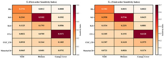
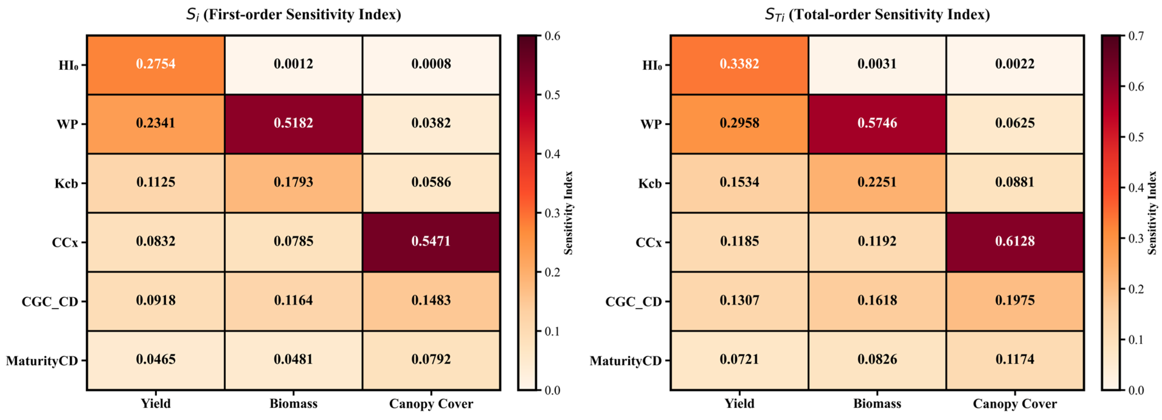
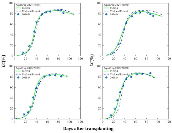
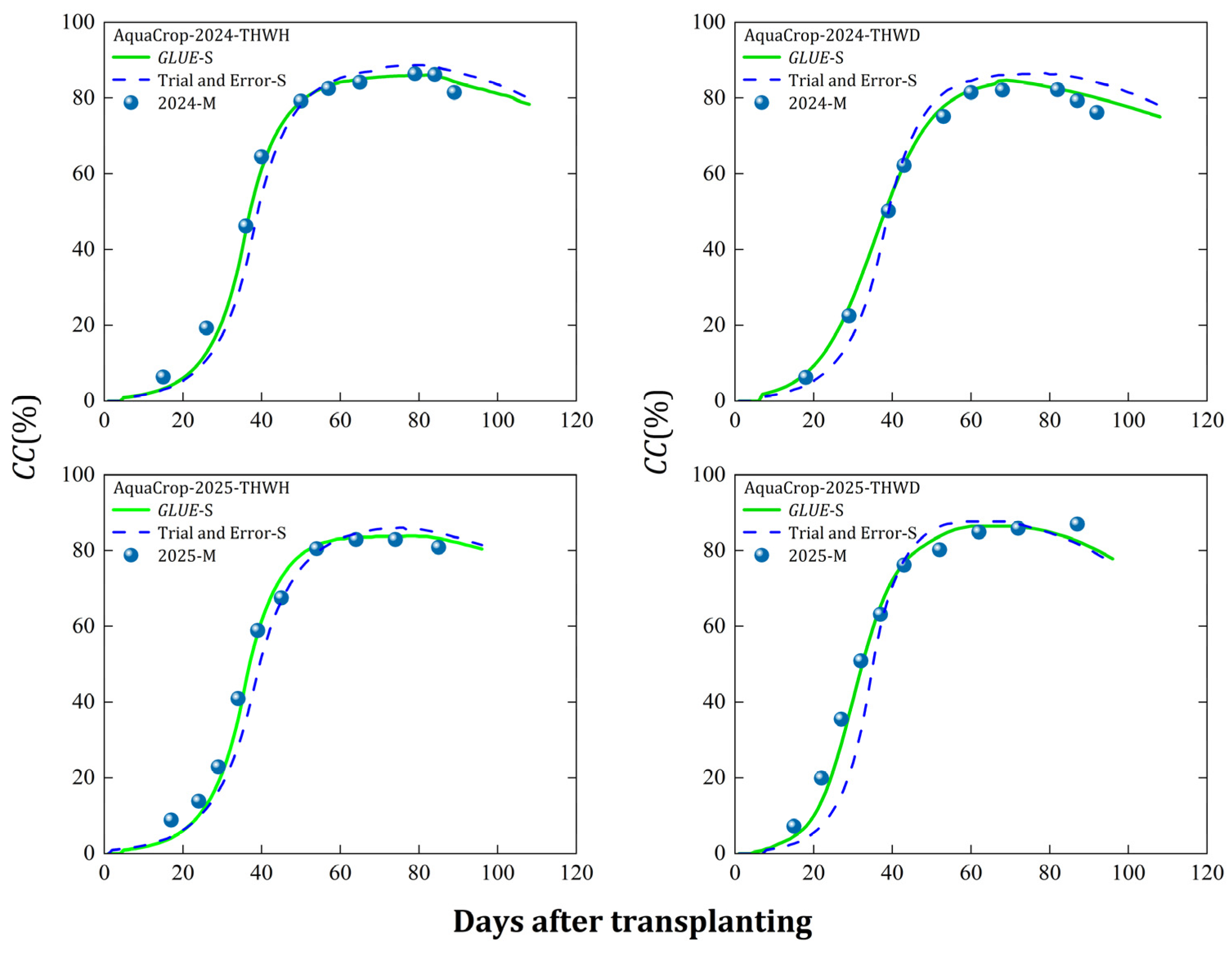
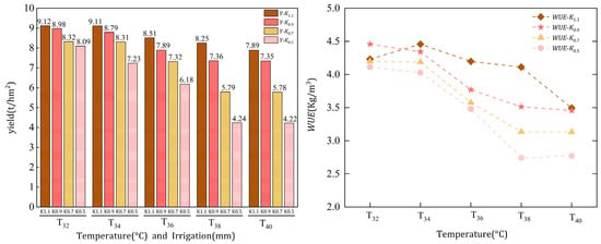
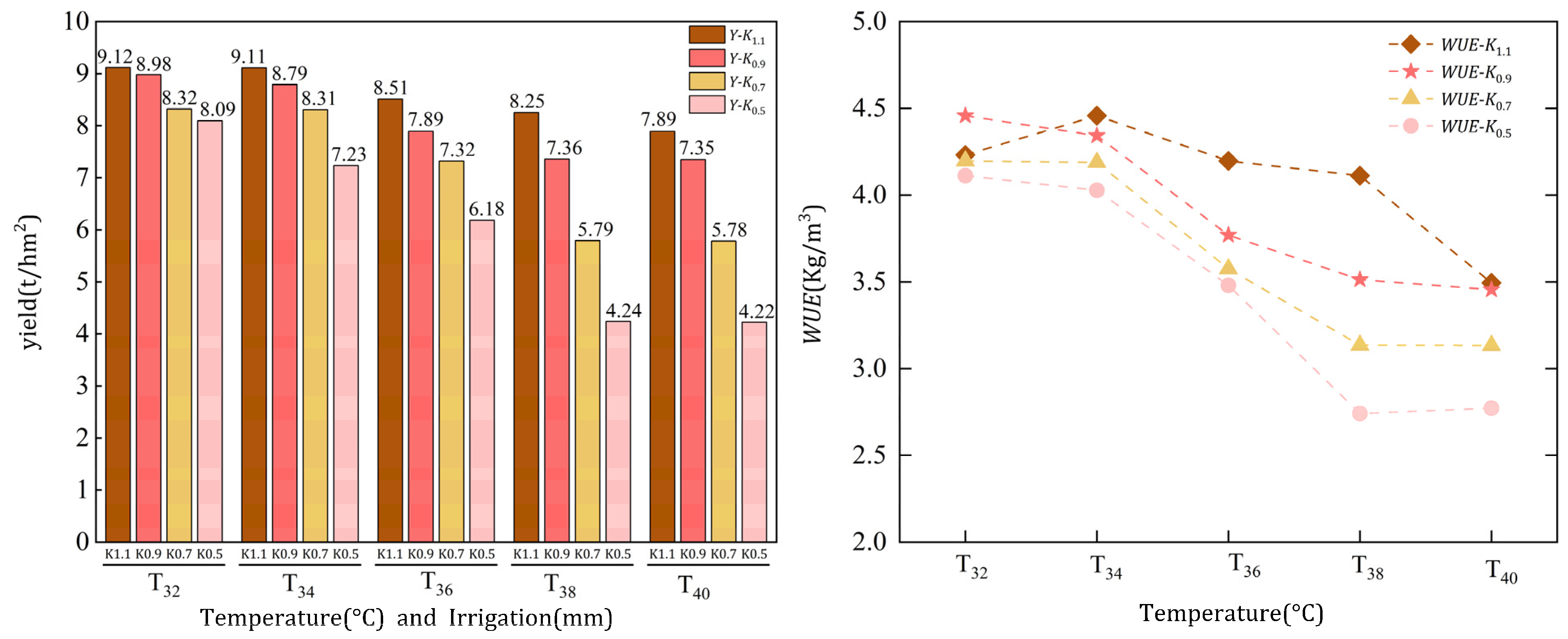

Disclaimer/Publisher’s Note: The statements, opinions and data contained in all publications are solely those of the individual author(s) and contributor(s) and not of MDPI and/or the editor(s). MDPI and/or the editor(s) disclaim responsibility for any injury to people or property resulting from any ideas, methods, instructions or products referred to in the content. |
© 2026 by the authors. Licensee MDPI, Basel, Switzerland. This article is an open access article distributed under the terms and conditions of the Creative Commons Attribution (CC BY) license.