


Abstract
Global olive oil consumption continues to grow, and Spain, particularly Andalusia, holds the largest cultivation area within the EU, covering 1.68 million hectares, which expanded by 7.7% between 2013 and 2023. However, precise data on the planting systems used are lacking; this information is essential for assessing crop intensification and its environmental, economic, and social implications. This study applies Deep Learning (DL) techniques to classify the planting system of olive parcels previously identified in a national cadastral database, using high-resolution RGB imagery acquired from a nationwide public aerial orthophotography program. Five DL algorithms (VGG19, InceptionV3, MobileNet, ResNet50, and Xception) were compared across different planting-system classification schemes and spatial resolutions, using a dataset of 8000 images (2000 per class) divided into training (70%), validation (20%), and testing (10%) subsets. The best results were obtained with a three-class scheme (traditional, intensive, and super-intensive) at 0.5 m/pixel resolution, reaching precision values of 99.00% with MobileNet and 98.66% with VGG19. These results support extending the approach to larger areas for regional-scale monitoring of planting systems, including other Mediterranean olive-growing regions, and provide a basis for further research on the water use and labor demand associated with each planting system.
1. Introduction
The Mediterranean region has been pivotal in the evolution and domestication of the olive tree (Olea europaea), establishing itself as the world’s leading supplier of olive oil to meet growing demand. Between 1995–1996 and 2019–2020, total consumption increased by 1.8 times [1]. This has driven a shift toward intensive cultivation systems characterized by high productivity. Olive orchard yields have increased substantially, from 500–600 kg/ha in traditional rainfed systems to 12,000–14,000 kg/ha in modern super-intensive systems [2]. However, the increased planting density and reduced spacing, while optimizing resource and land use, poses challenges in pest and disease management, labor requirements, light competition, and availability of water [3].
In 2022, the European Union (EU) accounted for two-thirds of the world’s olive oil production, with Spain contributing 63% of this output, covering 2.32 million hectares. Andalusia, the focus of this study, represents 72.6% of this area, accounting for 1.68 million hectares, with a 7.7% increase from 2013 to 2023 [4]. To support this expansion, intensified plantations with reduced tree spacing have been adopted. Traditionally, olive planting systems have been classified into three main categories based on planting density: traditional, intensive, and super-intensive [5]. Due to the growth of the super-intensive system, a new classification termed ’high-density intensive’ has been proposed [6], increasing the spacing between rows to reduce shading in the lower parts of the tree and decreasing the risk of disease without affecting long-term production. The specific density thresholds adopted for each class in this study are detailed in Section 2.3.
The growing adoption of more intensive plantations has progressively displaced traditional rainfed crops. This shift has increased input use, which has negatively impacted biodiversity and the ecological balance in various Mediterranean regions, including central Spain and southern Portugal [7,8,9]. Despite the potential benefits of olive intensification, it is crucial to address the challenges it poses to ensure long-term sustainability. This rapid evolution of olive cultivation systems has generated new challenges in terms of sustainability and efficiency. While intensification can increase productivity and carbon sequestration, it also demands higher irrigation and reduces labor needs, critical factors in arid and depopulated Mediterranean areas [10]. Furthermore, intensification typically requires greater fertilizer inputs, particularly nitrogen, phosphorus, and potassium, with the associated risk of over-fertilization, reduced oil quality, and environmental pollution if not properly managed [11], and has been associated with an increased incidence of pests and diseases, most notably Verticillium wilt, due to higher planting density and irrigation-related soil humidity [6]. To guarantee long-term sustainability, it is essential to address both the challenges of intensification and its impacts on rural livelihoods and community resilience. Recent studies highlight the importance of collecting farm-level data to optimize agricultural practices [12]. This shift has raised concerns among government institutions, which seek to legislate to improve the sustainability of agricultural systems and preserve crucial ecosystem services. The European Union (EU) and Spain have implemented significant policies such as the European Landscape Convention and the Common Agricultural Policy (CAP) 2023-27 to promote sustainable agricultural practices. In Spain, the CAP Strategic Plan (PEPAC) 2023–2027 emphasizes the importance of preserving traditional olive groves and those with high environmental value [13]. These initiatives underscore the need to develop effective tools for monitoring and classifying planting systems. Consequently, government institutions are seeking new tools to monitor and manage crops more efficiently.
In light of these challenges in sustainable olive grove management, there arises a need for advanced monitoring and classification tools. In this context, remote sensing (RS) has proven to be a versatile and efficient tool in olive growing, drawing on satellite, manned aerial, and unmanned aerial vehicle (UAV) platforms, each involving a different trade-off between spatial resolution, temporal frequency, and coverage area [14,15]. Satellite missions such as Sentinel-2 or Landsat provide frequent, low-cost coverage over wide areas, but their spatial resolution, typically 10 m or coarser, limits their ability to resolve individual tree crowns or fine-grained planting arrangements. UAV-based platforms can reach centimeter-level detail, sufficient for individual tree delineation and health assessment, but their limited coverage per flight and the logistical cost of repeated surveys constrain their suitability for regional-scale, recurring monitoring. Manned aerial photogrammetric programs, such as the one used in this study, occupy an intermediate position, providing sub-meter resolution over large national or regional extents at the cost of a lower revisit frequency than satellite or UAV platforms. However, processing the vast datasets generated by RS presents challenges for traditional classification methods [16,17,18,19]. This is where machine learning (ML) and deep learning (DL) become essential. ML identifies patterns and makes accurate predictions about crops, while DL, using deep neural networks such as convolutional neural networks (CNNs), significantly improves image classification. RS, combined with ML and DL, offers new perspectives for addressing the complexity of monitoring modern planting systems and opens the door to the creation of public statistics regarding the coverage and distribution of different olive planting systems. Its application in agriculture has facilitated advancements such as automated crop management [20]. Studies range from the identification of citrus trees [21,22] to the identification of hazelnut crops [23] and vine rows in terraced orchards [24]. Focusing on olive planting systems, studies such as [25] used image thresholding and Hough transform techniques to count olive trees in a plot and estimate production, achieving 98% accuracy in detecting olive tree crowns. In a related effort, ref. [26] compared five CNN architectures to classify the health status of olive trees from UAV imagery. On the other hand, more comprehensive studies, such as that of [27], employed the LeNet architecture to classify olive planting systems, achieving 97.5% accuracy at the sub-image level and 82% at the plot level.
These studies, however, leave gaps that are directly relevant to the operational monitoring of planting systems. First, ref. [25] relies on geometric image processing rather than learned representations, and [26] targets the health status of individual trees rather than planting structure, so neither addresses planting-system classification as such. Second, ref. [27], the only work to date that classifies olive planting systems with deep learning, is built on a single LeNet-based architecture, operates on aerial imagery at a single spatial resolution of 0.5 m, and adopts a single three-class taxonomy. Moreover, it classifies fixed-size image tiles individually and reconstructs a plot-level map by mosaicking the resulting predictions rather than assigning a class to the whole plot directly; the present study instead classifies each plot from a single whole-image input, without tiling or mosaicking. It therefore provides no evidence as to whether the reported performance depends on the architecture chosen, how it would be affected by finer or coarser imagery, or whether a four-class taxonomy that separates high-density intensive orchards remains separable from aerial imagery at all. Third, the drop from 97.5% accuracy at the sub-image level to 82% at the parcel level reported in that study indicates that patch-level performance does not transfer directly to the parcel, which is the unit on which agricultural statistics and policy instruments are actually built. This tiling strategy also requires one inference pass per tile plus a subsequent mosaicking step, increasing the computational cost relative to a single forward pass per plot and introducing an additional design choice—how predictions are reconciled across tile boundaries—that whole-plot classification avoids.
The primary objective of this study was to (a) compare the performance of five DL algorithms (MobileNet, InceptionV3, VGG19, ResNet50, and Xception) in classifying planting systems of olive parcels pre-identified through the SIGPAC database, (b) evaluate the impact of different image resolutions (0.5 and 0.25 m per pixel) on classification accuracy, and (c) analyze the effectiveness of three- and four-class classification schemes in capturing the diversity of current planting systems.
2. Materials and Methods
The workflow developed for the automatic classification of olive planting systems using deep learning techniques can be summarized in the following steps, described in detail in the subsequent sections: (1) selection of parcels containing olive orchards based on an official database; (2) extraction of aerial imagery corresponding to the selected parcels; (3) manual annotation of the extracted images; (4) training of various deep learning-based image classification algorithms; and (5) validation of the trained models. Two classification schemes were used throughout, clustering the extracted images according to a three-class and a four-class taxonomy of the planting systems, as detailed in Section 2.3.
2.1. Study Area
The present investigation incorporated olive orchard plots with different planting patterns located in Andalusia (southern Spain). The distribution of the plots was mainly concentrated along the Guadalquivir basin. Nevertheless, orchards from other areas were selected to ensure a representative sample and to include all the planting patterns to be studied. The geographical distribution of the study areas is delineated in Figure 1.
Figure 1.
Study site location (EPSG: 4326).
2.2. Data Sources
2.2.1. SIGPAC
The official database used for the selection of parcels containing olive orchards was the Geographic Information System for Agricultural Plots (SIGPAC) from [28], a database managed by the Spanish Agricultural Guarantee Fund (FEGA) and the agricultural departments of the autonomous regions. It allows for the geographic identification of agricultural plots declared by farmers for subsidy purposes under the Common Agricultural Policy (CAP). The system uses vector layers to provide detailed information about each plot, including its use and eligibility for subsidies. Olive parcel identification utilized SIGPAC database resources provided by the Andalusian Regional Government for 2017 and 2020, facilitating the identification of plantations registered within the CAP framework. These databases encompass comprehensive SIGPAC data through December 31, 2016, and 2019, respectively. The temporal consistency of PNOA imagery and SIGPAC information made possible the generation of an accurate training dataset.
2.2.2. PNOA
The imagery used in this study was sourced from the National Plan for Aerial Orthophotography (PNOA), managed by Spain’s National Geographic Institute (IGN). This program conducts nationwide aerial surveys with manned aircraft. PNOA imagery includes three multispectral bands, red (630–690 nm), green (520–600 nm), and blue (450–520 nm), with 8-bit radiometric resolution, and 36 scenes covering the study area were selected for analysis [29]. For dataset generation, orthomosaic images from the 2016 and 2019 flight campaigns, three years apart, were used, offering spatial resolutions of 0.5 m and 0.25 m per pixel, respectively.
2.3. Patterns for Olive Classification
The olive plantation classification methodology incorporated two distinct density-based taxonomic patterns, A and B. The primary classification framework (Pattern A), first defined by [6] and later applied by the Agricultural and Fisheries Research and Training Institute (IFAPA) [30], differentiates between traditional plantations (T), intensive plantations subdivided into low-density intensive (I) and high-density intensive (HDI), and super-intensive systems (SI). The secondary classification framework (Pattern B) consolidates these into three categorical designations: traditional (T), intensive (I), and super-intensive (SI), as described comprehensively by [3], who also provides a precise account of the classic plantation system classification.
Pattern A taxonomic criteria are defined as follows: (i) Traditional (T) olive orchards: characterized by expansive planting frameworks with inter-tree and inter-row spacing exceeding 7.5 m, maintaining densities lower than 204 trees/ha. (ii) Low-density intensive (I): exhibiting tree densities ranging from 204–600 trees/ha, with inter-tree spacing of 4–7 m and equivalent inter-row intervals. (iii) High-density intensive (HDI): comprising tree densities of 600–1000 trees/ha, with inter-tree spacing of 2–4 m and inter-row intervals of 4–7 m. (iv) Super-intensive (SI): characterized by inter-tree spacing of 1–2 m and inter-row intervals below 4 m, achieving densities of 1000–3000 trees/ha. In Pattern B, while traditional and super-intensive designations remain constant, both intensive subcategories are amalgamated into a unified intensive classification (I) in Table 1.
Table 1.
Density and spacing criteria for olive planting-system classification (Pattern A and Pattern B).
Note: In Pattern B, the Low-density intensive and High-density intensive classes are merged into a single Intensive (I) category (204–1000 trees/ha).
2.3.1. Classification Procedure
Figure 2 presents a schematic representation of the workflow implemented for the generation of the classification algorithm. The image extraction methodology comprised the following steps: (i) dataset generation through the identification of olive parcels using SIGPAC, parcel identification, and labeling [31]; (ii) centroid generation and image extraction with standardized dimensions of 299 × 299 pixels. The analytical process was then divided into four parallel streams based on the resolutions of the PNOA orthomosaics: (a) native 0.25 m resolution imagery; (b) native 0.5 m resolution imagery; (c) resampled imagery using the Nearest Neighbor technique in QGIS [3.40.15] (from 0.25 m to 0.5 m), selected because it preserves original pixel values without introducing interpolated artifacts and has been shown to yield classification performance comparable to more computationally intensive resampling approaches [32]; and (d) merging single-resolution datasets (0.25 m and 0.5 m) with the same planting pattern to create a multi-resolution dataset.
Figure 2.
Workflow for the generation of the classification algorithm.
2.3.2. Dataset Generation for Model Training
After selecting parcels containing olive orchards based on SIGPAC, the next step was to extract image patches of these parcels from PNOA in the size required by the classification algorithms. The cropping process was carried out by identifying the centroid of every olive orchard and drawing a square centered at this point with the desired dimensions of 299 × 299 pixels, as illustrated in Figure 3. Process automation was achieved through implementation of a custom PyQGIS script. Considering the differences in spatial resolution from 2016 and 2019 imagery, this cropping methodology resulted in coverage areas of 2.23 ha for the 2016 orthomosaics (0.5 m spatial resolution) and 0.56 ha for 2019 imagery (0.25 m spatial resolution).
Once the images were cropped, they were manually labelled by an expert through systematic visual inspection using QGIS. The images received two labels, each one according to one of the classification patterns previously detailed. According to Pattern A, the images were annotated as traditional, low-density intensive, high-density intensive, or super-intensive; according to Pattern B, the images were labelled as traditional, high-density and intensive, or super-intensive.
Figure 3.
Cropping methodology and results. (a,b) Real orthomosaic context for the 2016 (0.5 m) and 2019 (0.25 m) campaigns, respectively, showing centroid identification and buffer generation for the four planting systems (green: super-intensive; red: high-density intensive; blue: low-density intensive; orange: traditional). (c–f) Cropped samples at 0.5 m resolution (2016) for the super-intensive, high-density intensive, low-density intensive, and traditional systems, respectively. (g–j) Corresponding cropped samples at 0.25 m resolution (2019) for the same systems, in the same order.
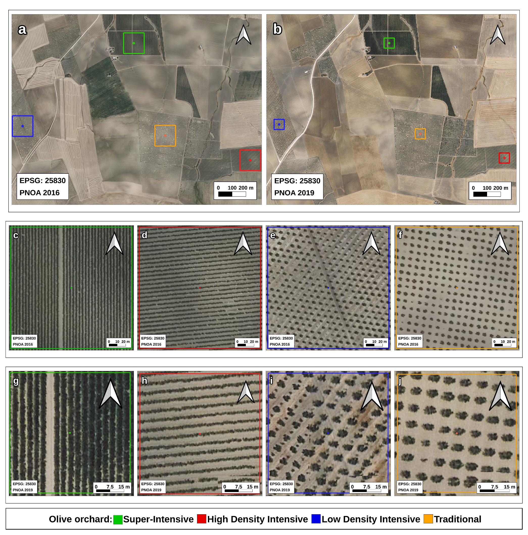
Since PNOA imagery from 2016 and 2019 had different spatial resolutions, this image property was considered in the generation of the datasets, creating both single-resolution (mono-resolution) and combined-resolution (multi-resolution) sets to simulate outcomes across various scenarios and to evaluate performance when input images have different resolutions. This approach aligns with prior studies [33] that demonstrated effective algorithmic training and validation across varying resolutions. Additionally, two datasets were obtained by resampling the 2019 images from 0.25 to 0.5 m resolution to evaluate whether image resolution or the data captured in a specific year influence the model’s performance. In this study, we analyzed whether a higher data density, understood as greater textural detail, could be counterproductive compared to the need to capture more contextual information. By modifying the resolution from 0.25 m to 0.5 m, the surface area analyzed by the model in each input window quadrupled, increasing from 0.56 ha to 2.23 ha. This increase is strategic, as it allows the neural network to process a much broader receptive field, facilitating the identification of geometric patterns and complete planting frameworks rather than overfitting to the variability of individual trees or shadows. This methodological decision was consistent with the recognized limitation of CNN architectures, whose inherently confined receptive field can impede the effective capture of extensive geographical features in remote-sensing imagery [34]. CNN-based models have proven effective at extracting the agricultural spatial structure from the textural transitions between and within fields in very-high-resolution imagery [35], supporting the choice of a broader spatial context to interpret the global and extended structure of the plantation. Therefore, using 0.5 m resolution optimized computational performance and ensured a more representative capture of contextual information for the classification of cropping systems. Finally, Table 2 details the specifications of the datasets according to the classification pattern used and the spatial resolution of the imagery.
Table 2.
Experimental design configuration for mono-resolution and multi-resolution dataset analysis.
The mono-resolution datasets (1–6) included approximately 8000 images for each resolution, while the multi-resolution datasets (7–8) contained approximately 16,000 images, created by merging two mono-resolution datasets. In datasets using Pattern A, each class was represented by a quarter of the samples. Datasets created according to Pattern B had one quarter of the samples for the traditional and super-intensive classes and two quarters for the ‘high-density and intensive’ class, as it results from merging two equally represented classes of Pattern A [33].
Data augmentation was applied to all datasets to account for the range of plot conditions encountered in the field [36]. Augmentation was implemented using the automated version generation engine within the Roboflow platform (Roboflow, Inc., Des Moines, IA, USA), where each source image in the training subset yielded three output versions, giving an expansion factor of 3× for the training set. Four methods were enabled, with the following configuration: a horizontal flip applied with 50 percent probability; a 90-degree rotation applied with equal probability across three states (none, clockwise, counter-clockwise); a Gaussian blur of between 0 and 1.25 pixels; and an exposure adjustment of between −15 and +15 percent. The partition was performed before any augmentation: the source image set was first divided into training (70%), validation (20%) and test (10%) subsets, and augmentation was subsequently applied exclusively to the training subset. Validation and test subsets therefore contain original, non-augmented imagery only. Class balance was enforced at dataset construction rather than at partitioning, as described above. Partitioning was performed randomly over the pooled set without explicit per-class stratification; because the source datasets were balanced by design, the resulting subsets preserved the intended class proportions with minor sampling variation. To verify the absence of leakage, we computed the pairwise intersections of source-image identifiers across the three partitions, and additionally of parcel-level identifiers, since multiple tiles may originate from the same parcel. All intersections were empty in both cases, confirming that neither augmented derivatives nor tiles from the same parcel are shared between the training, validation and test subsets.
2.3.3. Deep Learning Algorithms
The experimental framework utilized five deep learning (DL) architectures, selected for their proven success in agricultural image processing: MobileNet, VGG19, InceptionV3, ResNet 50, and Xception.
MobileNet is an efficient model for resource-constrained environments that use width and resolution multipliers to maintain precision while enhancing efficiency. It is based on depthwise separable convolutions, significantly reducing computational cost compared to standard convolutional networks. This architecture makes it particularly suitable for deployment on mobile and embedded devices without a substantial loss of accuracy [37]. Some authors have used it for classification and flowering recognition in agricultural applications [38].
Keras supports several state-of-the-art classifiers, including VGG19, InceptionV3, ResNet 50, and Xception, all of which have shown strong performance in agricultural applications. VGG19, introduced by [39], employs simple 3 × 3 convolutional layers and max-pooling operations for image classification tasks. Its efficacy was confirmed by [39] in a comparative study with VGG 16, processing over 160,000 images, and supported by [40,41] in agricultural contexts.
InceptionV3, with 48 layers, facilitates multi-scale feature extraction and resolution analysis for 299 × 299 pixel images, demonstrating superior performance [42]. It has been widely validated in agricultural applications [43], particularly for plant classification and pathology detection [37,44].
ResNet 50, introduced by [45], employs residual modules that enable effective training of deep networks through skip connections and global average pooling. This architecture has been successful in crop classification and soil analysis using multispectral imagery [46].
Xception, proposed by [47], extends Inception by using depthwise separable convolutions, achieving reduced parameter size while maintaining outstanding performance. However, it requires 299 × 299 pixel image inputs, similar to Inception V3. It outperforms VGG 16 and Inception V3 in plant pathology identification [48] and has demonstrated classification accuracy exceeding 97% in maize cultivation [49].
All five architectures were instantiated from Keras Applications with ImageNet-pretrained weights and without their top classification layers, obtained from the public Keras Applications repository (https://storage.googleapis.com/tensorflow/keras-applications/, accessed on 17 August 2026).
The models were applied through transfer learning [50]: the convolutional layers of the pretrained backbones were kept frozen, and only the final dense classification layer was trained, so that the networks operated as fixed feature extractors. This approach reuses the prior capacity of the models to recognize learned visual patterns, facilitating their adaptation to a new classification task without modifying the pretrained representations.
The computational implementation was executed on Google Colab Pro (Google LLC, Mountain View, CA, USA)’s infrastructure, employing a Tesla P100 GPU with 16 GB VRAM and 16 GB RAM. All architectures shared an identical training configuration for batch size (32), loss function (Sparse Categorical Crossentropy [51]), and the Adam optimizer with its default parameters (learning rate = 0.001, β1 = 0.9, β2 = 0.999, ε = 1 × 10⁻⁷) [52]. Training was capped at 500 epochs [53] and regulated by an early stopping criterion monitoring validation loss (mode = min, patience = 5 epochs); the final weights correspond to the last epoch executed rather than to the epoch of minimum validation loss, as weight restoration was not enabled. Input images were resized as required by each architecture: 224 × 224 × 3 for VGG19, MobileNet, and ResNet50, and 299 × 299 × 3 (matching the extracted tile size, without resizing) for InceptionV3 and Xception, all rescaled to [0, 1]. No fixed random seed was set during training; consequently, exact numerical reproducibility for individual runs is not guaranteed, although the relative performance of the architectures was consistent across the eight datasets evaluated. Model selection during development was guided by accuracy, while the comparative evaluation reported in Section 3 relies on the metrics described in Section 2.3.4 [54]. The complete configuration is summarized in Table 3.
Table 3.
Training hyperparameters for the five deep learning architectures.
2.3.4. Validation Methodology
Model validation encompassed a rigorous evaluation protocol to assess the effectiveness of the trained architectures under the previously specified parameters. The validation methodology implemented a comparative analysis between predicted outputs and ground truth labels from the test set, yielding key performance indicators: True Positives (TPs), True Negatives (TNs), False Positives (FPs), and False Negatives (FNs). Following the methodological framework widely adopted by many authors for the evaluation of deep learning models [55], these foundational metrics were utilized to compute comprehensive performance indicators. The evaluation framework incorporated precision metrics to quantify the ratio of correct positive predictions relative to total positive predictions, while recall measurements assessed the model’s capacity for positive case identification. The F1-Score was computed as the harmonic means of precision and recall metrics, providing a balanced metric of performance. Overall model performance was assessed using accuracy metrics, representing the proportion of correct predictions across the total prediction set. The mathematical formulation and detailed metric specifications are delineated in Table 4.
Table 4.
Mathematical definitions and formulas for evaluation parameters.
To evaluate the datasets, the precision Equation (1), recall Equation (2), and F1-Score Equation (3) results from the models must be averaged. This makes it possible to determine which dataset performs better, regardless of the model used. It also allows for the assessment of whether Pattern A or B is the optimal combination, as well as identifying the most suitable resolution in each.
To compare models, the macro F1-Score metric was used in Equation (4), which has also been employed by other authors to evaluate models in multiclass problems [56]. This metric computes a simple average of the F1-Score calculated independently for each class, where N is the number of classes and F1i corresponds to the F1-Score of class ‘i’. This approach treats all classes equally, measuring the overall performance of the model without favoring the most frequent classes, even when the datasets have different class distributions.
The four best-performing models from datasets 1 to 6, developed independently for patterns A and B at spatial resolutions of 0.25 m and 0.5 m, were identified for this analysis. Each of these models was tested using input data at the alternate resolution to the one used for training (Table 5). This procedure aimed to assess the robustness and generalization capability of the models when exposed to spatial resolutions differing from those encountered during training. Accordingly, four independent evaluation scenarios were conducted: models trained at 0.25 m for both patterns A and B were tested on imagery at 0.5 m, and conversely, models trained at 0.5 m were tested on imagery at 0.25 m.
Table 5.
Assessment to evaluate the generalization capacity of the best-performing models on spatial resolutions outside their training domain.
2.3.5. Experimental Design and Statistical Description
The experimental design comprised eight datasets (Table 2), resulting from the combination of two classification patterns (A, four classes; B, three classes), two spatial resolutions (0.25 m and 0.5 m, native and resampled), and a multi-resolution merge. Each dataset was partitioned following a 70-20-10 ratio for training, validation, and testing. No repeated measures or blocking structure was applied, as each image constituted an independent experimental unit. Model training and evaluation were implemented in Python [3.13], using Keras [3.13.0] as the high-level API for TensorFlow [2.20.0]. Image extraction and geoprocessing were performed in QGIS [3.40.15] using a custom PyQGIS script. Performance was assessed using precision, recall, F1-Score, and accuracy, as defined in Table 2.
3. Results
3.1. Analysis of the Validation Metrics to Evaluate the Datasets and Identify the Best General-Purpose Model
The DL algorithms classified planting systems with an average precision of 90.35% for Pattern A at 0.5 m resolution, and 85.10% at 0.25 m resolution (Table 6). For the Pattern B setup, precision was higher at 0.5 m and 0.25 m, reaching values of 98.26% and 95.26%, respectively. When orthomosaics at 0.5 m/pixel were used, model performance was higher than at 0.25 m, regardless of the pattern: 94.30%, corresponding to datasets 1 and 3, compared to 90.18%, corresponding to datasets 2 and 4, an increase of 4.12%.
As previously explained, datasets 5 and 6 were created by downsampling datasets 2 and 4 from 0.25 to 0.5 m spatial resolution. Decreasing the resolution did not improve the results, but they dropped from 90.18% (datasets 2 and 4) to 87.23% corresponding to datasets 5 and 6, around 3%. Regardless of resolution and without downsampling, Pattern A achieved a precision of 87.72%, corresponding to datasets 1 and 2, whereas Pattern B attained 96.76%, corresponding to datasets 3 and 4, which was approximately 9% higher.
Overall, the standard deviation is low, indicating that all models exhibit similar behavior across datasets. Only for datasets 4 and 8 did the standard deviation slightly exceed 2%, while for the remaining datasets it remained below 1%.
Table 6.
Average precision of the dataset design (Pattern A or B).
In general, the models predicting Pattern B, corresponding to datasets 3, 4, 6, and 8, achieved a higher average recall (92.09%) compared to those designed for Pattern A, corresponding to datasets 1, 2, 5, and 7 (87.28%) (Table 7). Certainly, models with three classes performed significantly better, regardless of resolution. When considering single-resolution setups independently of the number of classes and resampling strategies, models with datasets 1 and 3 with a spatial resolution of 0.5 m outperformed models with datasets 2 and 4 with a spatial resolution of 0.25 m by approximately 3%. Dataset 3, with a spatial resolution of 0.5 m and three classes, consistently yielded substantially better results than all others, regardless of the model used.
Regarding the resampled datasets, like the precision metric, recall decreased by approximately 5%, except for dataset 5, which showed results comparable to dataset 2, with similar recall. Concerning the multi-resolution setting, models with Pattern B yielded better results than those with Pattern A. As observed with precision, combining different resolutions and increasing the number of classes led to improved performance.
Table 7.
Average recall of the dataset design (Pattern A or B).
Dataset 3 appeared to be the least challenging, with minimal variability under the configuration of three classes and a 0.5 m resolution: all models achieved F1-Scores above 95%. Dataset 7 had the lowest observed standard deviation, indicating highly consistent results across architectures, and also yielded high performance across all models, with F1-Score values over 89%. Dataset 4 exhibited the higher standard deviation, primarily due to the performance of ResNet50, which consistently achieved lower F1-Scores compared to the other models. Overall, Pattern A with resampled resolutions of 0.25 and 0.5 m (datasets 2 and 5) yielded the lowest results, with similar performance between them. Notably, dataset 5 did not achieve results comparable to dataset 1, despite being a resampled version. The best performance for Pattern A was observed with the original dataset 1 configuration. In contrast, Pattern B generally produced higher scores than Pattern A, with the best combination obtained at a resolution of 0.5 m.
3.2. Macro F1-Score for the Evaluated Models
The macro F1-Score was computed for each model, along with the mean and standard deviation of F1-Score across all datasets (Table 8). Among the models evaluated, VGG19 and MobileNet stood out with the highest overall performance, achieving average macro F1-Scores of 90.22% and 89.96%, respectively. Although VGG19 showed the best overall performance, MobileNet outperformed it in several datasets. In contrast, ResNet50 obtained the lowest overall performance, with a mean macro F1-Score of 87.46%, approximately 3.5 percentage points lower than the top-performing models. Inception V3 and Xception exhibited intermediate results, with relatively consistent, though not outstanding, performance.
Table 8.
Average F1-Score of the dataset design (Pattern A or B).
3.3. Class-Wise Analysis of the Results
3.3.1. Class-Wise Results for Pattern A
Figure 4 presents the precision, recall and F1-Score values at class level for the 4 classes in Pattern A. The super-intensive and high-density classes yielded similar F1-Scores for both 0.5 m and 0.25 m spatial resolutions (Figure 4). For the intensive and traditional classes, a decrease in F1-Score of nearly 12% was observed when moving from 0.5 m to 0.25 m resolution for all models. When the image was resampled to 0.5 m, only the traditional class showed an improvement in performance across all models except for ResNet50; for the remaining three classes, F1-Scores decreased. According to the confusion matrices of the five models across these four datasets (Appendix A, Table A1, Table A2, Table A3 and Table A7), misclassifications primarily occurred between adjacent classes—those with similar planting frame structures above or below the target class. An exception was the traditional class, which was only misclassified with the super-intensive class in very isolated cases.
Figure 4.
Class-wise precision, recall, and F1-score for Pattern A (four classes) across spatial resolutions. (a.1–a.4) Precision for the super-intensive, high-density, intensive, and traditional classes, respectively. (b.1–b.4) Recall for the same four classes, in the same order. (c.1–c.4) F1-score for the same four classes, in the same order.
When both 0.25 m and 0.5 m datasets were combined, the resulting performance exceeded that of using only the 0.25 m dataset and was comparable to training exclusively on the 0.5 m dataset. The confusion pattern remained consistent, with most errors occurring between the most visually or structurally similar classes.
The class-wise analysis revealed that, for the super-intensive class, MobileNet model stood out by achieving the highest precision of 99% in the dataset, with a resolution of 0.5 m per pixel, accompanied by a recall of approximately 80%. This indicates that the model makes highly confident predictions when it detects a pattern, but it may miss some true positives. In contrast, VGG19 and Xception offered a more balanced performance between precision and recall, resulting in F1-Scores between 88% and 89%. Under multi-resolution conditions, a slight decrease in F1-Score was observed across most models. For the high-density class, a greater variability in performance was observed among the models. VGG19 and MobileNet consistently achieved high precision values, while the best F1-Score was shared between InceptionV3 and ResNet50, depending on the dataset.
In the case of intensive olive orchards, the classification performance showed greater robustness. MobileNet and Xception achieved F1-Scores close to or exceeding 90% across all datasets. This class was also characterized by high recall values in most models, indicating strong sensitivity in detecting this planting configuration. Traditional olive orchards exhibited the best overall results. Models such as Xception and VGG19 achieved F1-Scores between 95% and 99%, even under resampling or multi-resolution conditions. In addition, precision values were consistently high across all models.
3.3.2. Class-Wise Results for Pattern B
Figure 5 details the values of precision, recall and F1-Score at class level for the three classes in Pattern B; the corresponding confusion matrices are reported in Appendix A (Table A4, Table A5, Table A6 and Table A8). In this pattern, which involves the merging of two classes into a single category, a general improvement in performance was observed when using a spatial resolution of 0.5 m, yielding results (Figure 5) that surpassed those obtained with Pattern A. In fact, this configuration represented the most effective combination across all experiments, with all models achieving F1-Scores exceeding 95% for every class. When employing a finer resolution of 0.25 m, performance remained similarly high, with all models and classes attaining F1-Scores above 90%. However, when the 0.25 m data was resampled to a coarser 0.5 m resolution, a consistent decrease in performance was observed, approximately 10%, particularly in the super-intensive class and in the merged class comprising intensive and high-density categories. Conversely, the traditional class maintained the same performance levels observed at the native 0.5 m resolution. When combining datasets from different years and resolutions, the predictive performance for the intermediate and traditional classes tended to decline, whereas the super-intensive class retained high accuracy across most models, except for MobileNet, which exhibited a notable drop in F1-Score.
Figure 5.
Class-wise precision, recall, and F1-score for Pattern B (three classes) across spatial resolutions. (a.1–a.3) Precision for the super-intensive, high-density & intensive, and traditional classes, respectively. (b.1–b.3) Recall for the same three classes, in the same order. (c.1–c.3) F1-score for the same three classes, in the same order.
All models achieved high performance across all datasets for the super-intensive class. In the datasets, ResNet50 reached the highest score, with an F1 of 100%, while other models also maintained F1-Scores above 96%. In the higher resolution, the results remained excellent, with MobileNet and Xception displaying a particularly good balance between precision and recall (F1 ≈ 99%). After resampling, a performance reduction was observed in all models. Under multi-resolution conditions, a slight decrease in F1-Scores was observed across all models, likely due to increased spatial variability. In dataset 3 and dataset 4, all models achieved F1-Scores between 97% and 99%. However, with the resampled dataset, greater variation emerged, particularly in ResNet50, which dropped to F1 = 87%. In the multi-resolution dataset, some models showed reduced precision, although recall remained high. As a result, MobileNet and Xception continued to perform reliably, with F1-Scores between 93% and 97%. The traditional class showed the highest and most consistent results overall. All models performed exceptionally well in dataset 3 and dataset 4, with F1-Scores ranging from 97% to 99%. In the resampled dataset, ResNet50 experienced a moderate decrease (F1 = 89%), while the other models maintained strong performance. Under multi-resolution conditions, a minor drop in performance was noted, but VGG19 and Xception sustained high F1-Scores (98–99%), confirming their robustness. Across all configurations, the merged ‘intensive and high-density’ class, which accounts for approximately twice the sample count of each remaining class, did not obtain higher per-class scores than the two minority classes: the three categories fell within a comparable F1 range, and the single highest value (F1 = 100%, ResNet50) corresponded to the super-intensive class, which represents approximately one quarter of the samples. This indicates that the class imbalance introduced by the merge in Pattern B does not bias performance towards the over-represented class.
3.4. Validation of the Best-Performing Models on Unseen Data
Finally, to assess whether the models were able to predict at a spatial resolution different from that used during training, the two best-performing models according to the macro F1-Score, VGG19 and MobileNet, corresponding to Patterns A and B, respectively, were evaluated on unseen data. The VGG19-based model was trained using 0.5 m resolution data and tested with 0.25 m resolution inputs, and vice versa.
3.4.1. Results Using Pattern A
When VGG19 was tested on 0.5 m resolution data, the model achieved high precision (97%) but low recall (58%) for the super-intensive class (Table 9; confusion matrices in Appendix A, Table A9 and Table A10). This indicates that while the model was highly accurate in predicting the super-intensive class, it frequently failed to detect it, often misclassifying 33% of such instances as high-density and 7% as intensive. For the high-density class, the model demonstrated good sensitivity (recall) but tended to misclassify a considerable number of samples belonging to this category. The intensive class yielded a balanced performance with an F1-Score of 81%, representing the most stable behavior among the four classes regardless of resolution. Meanwhile, the traditional class was detected with high reliability regardless of the training resolution, suggesting it is easily distinguishable.
When trained on 0.5 m resolution data and tested with inputs at 0.25 m, the VGG19 model showed a decrease in precision but a substantial improvement in recall (+24%) for the super-intensive class, indicating improved ability to detect this plantation. For the high-density and intensive classes, precision increased slightly while recall decreased, resulting in a compensatory effect that preserved the F1-Score. The performance for the traditional class remained comparable to the previous evaluation, confirming its consistent detectability across spatial resolutions.
Table 9.
VGG19, the top-performing model for Pattern A under untrained resolution conditions.
3.4.2. Results for Pattern B
For Pattern B and MobileNet (Table 10; confusion matrices in Appendix A, Table A11 and Table A12), when predictions were made on 0.5 m resolution data using a model trained on 0.25 m data, the model frequently misclassified the super-intensive class. However, performance improved after merging the intermediate classes following a trend like the previously described scenario. As before, predictions for the traditional class remained highly reliable, with the model correctly identifying most true cases.
When the resolutions were reversed, overall performance improved when the model was trained on 0.5 m data. Nevertheless, across all scenarios, metrics consistently declined when the model was evaluated at a resolution different from the one used during training, whether under a single-resolution or multi-resolution setting.
Table 10.
MobileNet, the top-performing model for Pattern B under untrained resolution conditions.
3.4.3. Effect of Spatial Resolution on Receptive Field and Crown Texture
The asymmetric degradation observed in Section 3.4.1 and Section 3.4.2 can be explained by the interaction between the fixed receptive field of the networks and the variable ground extent represented by each pixel. Image tiles were extracted at 299 × 299 pixels and resampled to the 224 × 224 input used for all architectures, so that each input pixel corresponds to 1.33 pixels of the source imagery. The theoretical receptive field of the VGG19 backbone, computed layer by layer from kernel sizes, strides and pooling operations, is reported in Table 11.
Table 11.
Theoretical receptive field of the VGG19 backbone by convolutional block, expressed in input pixels, source-image pixels, and ground distance at 0.25 m and 0.5 m spatial resolution.
The receptive field is constant in pixel units, at 268 input pixels at the output of the final convolutional block, but the ground extent it covers depends on the resolution of the source imagery: approximately 89 m at 0.25 m resolution and 179 m at 0.5 m. In both cases it exceeds the 299-pixel extent of the extracted tile, so units at the final convolutional stage integrate the entire tile (74.8 m at 0.25 m resolution and 149.5 m at 0.5 m), with sensitivity decaying towards the periphery. A model trained at one resolution therefore applies filters calibrated for a spatial context that represents twice the ground extent when transferred to the other.
The same scaling governs crown texture. The inter-tree spacing that defines each planting system (Table 1) spans a different number of pixels at each resolution, as summarized in Table 12.
Table 12.
Inter-tree spacing of each planting system expressed in pixels at the two spatial resolutions.
The intrinsic image mechanism responsible for the accuracy decline in the super-intensive class is quantitatively explained by the interplay between the receptive field and the inter-tree spacing. A resolution degradation from 0.25 m to 0.5 m reduces the gap between super-intensive trees to 2–4 pixels. Consequently, adjacent crowns merge into a continuous textural block already at the image level, before any convolutional processing, and the network loses the ability to delineate individual tree boundaries. This directly explains the significant drop in recall observed for this class under cross-resolution evaluation, while precision remains high. By contrast, the traditional class retains more than 15 pixels between trees at both resolutions, consistent with the stability of its per-class metrics across all cross-resolution scenarios. Figure 3 presents visual comparisons of the exact same plot at both spatial resolutions for each planting system, illustrating the distortion of crown texture features and the geometric limitations highlighted by the receptive field analysis.
4. Discussion
Earlier work on olive planting-system classification has generally addressed planting density or a single architecture in isolation. The present study was designed to examine several of these factors jointly, namely the spatial relationship between trees, canopy size, and planting structure, by evaluating five deep learning architectures across image resolutions and classification schemes. The following sections discuss these results in relation to prior approaches (Section 4.1), the effect of spatial resolution and classification granularity (Section 4.2), architecture-specific performance (Section 4.3), cross-resolution generalization (Section 4.4), and directions for future work (Section 4.5).
4.1. Comparison with Previous Approaches to Planting-System Classification
Some authors have already applied deep learning models to classify olive grove planting patterns using orthophotos, but only for Pattern B [27]. To do so, they estimated the canopy cover fraction (FCC) and, based on this value, determined the type of planting pattern. However, this methodology presents certain limitations, such as the inclusion of weeds and cover crops, which introduces errors, especially considering that the current Common Agricultural Policy [13] encourages the presence of vegetation between trees to qualify for green payment schemes, which may further distort the FCC calculation. Notably, while [27] reported 82% accuracy at the plot level for Pattern B using an FCC-based approach with LeNet, the present study achieved a mean precision of 98.26% for the equivalent three-class configuration at 0.5 m resolution (dataset 3), suggesting that a direct classification approach based on spatial pattern recognition may be less sensitive to the FCC-related confounds discussed above. More recently, the same research group extended this line of work to medium-resolution satellite imagery, evaluating three CNN strategies (resizing, cropping, and fully convolutional networks) on Sentinel-2 data at 10 m and reporting a best overall accuracy of 80.6% for the three-class scheme [57]. That study argues that the temporal advantage of Sentinel-2, with a five-day revisit against the multi-year cycle of aerial orthophotography, offsets the loss of spatial detail, on the grounds that its accuracy is comparable to that previously obtained from 0.5 m orthophotos. The present results qualify that conclusion. Using direct spatial-pattern recognition rather than a canopy-cover-fraction proxy, the three-class scheme at 0.5 m reached an overall accuracy of 98.3% with VGG19 and 98.9% with MobileNet (Appendix A, Table A4), roughly 18 percentage points above the Sentinel-2 result and well above the 82% previously reported at the same spatial resolution. The apparent equivalence between 10 m and 0.5 m imagery therefore appears to be a property of the classification strategy rather than of the imagery itself: once the classifier exploits the geometric arrangement of the orchard, spatial resolution becomes decisive again, and the trade-off between spatial and temporal resolution must be reassessed accordingly. Other recent satellite-based studies have addressed adjacent aspects of olive orchard structure without performing the direct, multi-class planting-pattern classification undertaken here. Ref. [58] estimated olive tree density in Extremadura, Spain, from 435 samples obtained by detecting and counting individual trees via object detection on native-resolution PNOA orthophotos and then transferred the resulting density values to Sentinel-2 spectral bands via Random Forest regression; density, not planting-system class, was the output, and no parcel-level architecture was classified. Ref. [59] mapped the emergence of super-intensive olive plantations in Morocco using unsupervised satellite-based clustering but detected only that single class, from a comparatively small reference sample, rather than discriminating across the full range of planting patterns addressed by the present taxonomy. Other authors also performed tree counting using machine learning algorithms, but only for olive groves with discontinuous canopy cover, which prevents subsequent classification of the planting pattern in classes with continuous canopy [60]. Some researchers have proposed methodologies for distinguishing olive tree canopies, weeds, etc., but they require high-resolution RGB or multispectral UAV imagery [61], which limits the applicability of such approaches to large-scale areas for decision-making purposes. In this context, there is a need for high-level territorial analysis based on open data that supports decision-making. A high temporal resolution is not necessarily required, as previous studies have shown that monitoring programs with high spatial resolution and low temporal frequency can effectively assess large-scale temporal trends [62]. This suggests that, for certain macro-level analyses, a reduced temporal frequency of three years, like the one for the PNOA imagery used in this work, does not compromise the reliability of the conclusions.
4.2. Effect of Spatial Resolution and Classification Pattern on Model Performance
The spatial resolution of images has been recognized as a critical factor influencing classification performance across a wide range of remote sensing and computer vision applications. In this context, previous work has shown that spatial resolution requirements are specific to the application and the landscape being studied, rather than universal, and has proposed frameworks to guide such requirements [63]. Research has also shown that variations in image resolution can adversely affect the performance of convolutional neural network (CNN)-based classifiers, ultimately reducing the accuracy of the results [64]. In the present study, it was observed that, for any planting pattern, models trained with lower-resolution images achieved better performance metrics. This finding can be explained by two factors. First, since the input dimensions are limited to 299 × 299 pixels, images with a resolution of 0.5 m covered an agricultural area more than four times larger than that of 0.25 m resolution images, meaning the model received a broader territorial context as input, albeit with less detail. Second, it has been argued that the use of low-resolution imagery can facilitate both the distribution and training of deep learning models by reducing the risk of overfitting and focusing the learning process on high-level features, as is the case with planting pattern classification [65]. However, in datasets five and six, for which the resolution was reduced to 0.5 m through resampling, no improvement was observed compared to the results from the 0.25 m resolution. When considering both Pattern A and Pattern B, the latter consistently yielded better results, approximately 6% higher, regardless of spatial resolution. According to [3], Pattern B is the most used for defining olive grove planting frameworks, whereas [6] supports the use of Pattern A based on the analysis of canopy continuity. In this context, traditional and intensive plantations, which exhibit a discontinuous canopy structure as described by Pattern A, are more easily detected than those with a continuous canopy, such as high-density and super-intensive plantations, where canopy tangency can sometimes be observed. This continuity appeared to have a direct impact on the model’s ability to distinguish between patterns, which was reflected in the classification of outcomes. In fact, the confusion matrix of the best-performing model for Pattern A, VGG19, showed that most classification errors occurred between adjacent classes in terms of canopy continuity. The inferior performance observed for Pattern A, compared to Pattern B, may be attributed to a higher complexity in the decision space, which increased the likelihood of class confusion, as previously noted in the literature.
4.3. Architecture-Specific Performance: VGG19 and MobileNet
Pattern A was a classification scheme that performed well using both 0.25 m and 0.5 m spatial resolutions in a single-resolution setup. Classes with a higher number of trees per unit area benefit more from the 0.25 m resolution, as they require greater spatial detail to distinguish individual canopy structures. In contrast, classes with fewer trees per unit area achieved better results at 0.5 m resolution, which provides a broader spatial context that enhances the recognition of regular planting patterns. So, images at 0.25 m contain approximately 90 olive trees, whereas those at 0.5 m display around 400, which allowed for a clearer visualization of planting patterns in frameworks with fewer trees. This behavior was confirmed when applying resampling from 0.25 to 0.5 m, where an improvement was observed exclusively in the performance of the traditional class, with its F1-Score increasing from 84 to 91. This result suggests that this class was the most dependent on a larger surface area for the correct detection of the planting framework. This finding aligns with what is reported in [19], where the need for high-level contextual information is emphasized as essential for optimizing model performance.
In the case of Pattern A and the classes with continuous canopy (high-density and super-intensive), the opposite behavior was observed: the results improved with increasing resolution, with the F1-Score rising from 87 to 90 for both classes. Several authors have pointed out that, in certain situations, increasing the resolution can enhance [63,66] model performance when a higher level of detail is required, which corresponds to the case of continuous canopy classes. Conversely, when the model is trained to classify only three classes, as in the case of Pattern B, the impact of spatial resolution became less significant. This is because the reduced number of planting framework categories simplifies the classification task, resulting in more stable performance metrics regardless of the resolution used.
The results indicated that single-resolution configurations outperform multi-resolution approaches. Therefore, considering that both resolutions yielded satisfactory results for low-density planting frameworks, and for high-density the results were better at 0.25 m resolution, the combination of 0.25 m imagery and the VGG19 architecture emerges as a preferable option for Pattern A.
One possible reason why VGG19 outperformed more modern architectures such as MobileNet, Xception, InceptionV3, and ResNet50 in this specific task lies in its architectural simplicity and uniform depth, characteristics that have already shown great effectiveness in other agricultural applications. A recent study confirmed the robustness of VGG19 for vegetation feature extraction and classification in images captured by unmanned aerial vehicles (UAVs) [67]. As described in the methodology, its reliance on small 3 × 3 filters allows for consistent spatial feature extraction. This characteristic may be particularly advantageous when dealing with regular and repetitive spatial patterns, such as tree rows in olive groves, where deeper but more complex or fragmented architectures might overlook the broader structural regularities or overfit to fine-grained noise. In contrast, the controlled complexity of VGG19 may help maintain a balance between abstraction and spatial coherence. This full-tile integration is consistent with the discriminative capacity observed for planting patterns, whose characteristic spacing is resolved by intermediate blocks 3 and 4 (17–41 m at 0.25 m resolution; Table 11).
Considering Pattern B, the best performance was observed at 0.5 m, likely because there is only one high-density class, super-intensive, which was not easily confused with the intensive or traditional classes. Moreover, the latter two were best detected at 0.5 m, as previously demonstrated. Therefore, 0.5 m resolution emerges as the optimal choice for Pattern B. MobileNet may perform better with lower-resolution imagery due to its lightweight architecture, which is specifically optimized for efficiency in environments with limited computational resources and reduced input dimensionality [68]. Unlike deeper or more complex networks, MobileNet employs depthwise separable convolutions that reduce the number of parameters and operations, allowing it to generalize more effectively when fine spatial details are limited [69]. In scenarios involving lower-resolution images, where high-frequency features are inherently less available, MobileNet’s design focuses the learning process on broader, more abstract patterns, which can be advantageous for tasks such as planting pattern classification [70], which relies on contextual and structural cues rather than fine-grained texture. As a result, MobileNet’s simplicity becomes an asset under reduced spatial resolution conditions and fewer classes.
4.4. Generalization Across Training and Inference Resolutions
Regarding inference at resolutions different from those used during training, the present results show that classification metrics consistently declined whenever the evaluation resolution differed from the training resolution (Table 10 and Table 11). This is consistent with the features learned by each model being adapted to the scale at which the planting structure was presented during training. A train–test resolution discrepancy has also been documented in general-purpose image classification by Touvron et al. [71], who showed that standard data augmentation causes objects to appear at different apparent sizes at training and test time, and who addressed it by fine-tuning the classifier at the test resolution rather than by matching the two resolutions. Their setting is not directly transferable to the present case: they varied the pixel dimensions of the network input while the scale of the imaged objects remained fixed, whereas here the extracted tile size was fixed at 299 × 299 pixels for every architecture (Section 2.3.3), and it was the ground sampling distance, and therefore both the ground area covered and the apparent size of the planting framework, that changed. Fine-tuning at the evaluation resolution was not performed in this study; it constitutes a plausible route to mitigate the observed degradation and remains to be tested, together with the influence of the resampling method used to convert between spatial resolutions.
To further characterize the resolution-driven decline reported above, we quantified the underlying texture and periodicity differences, focusing on the super-intensive class, where the effect is largest, and on the same four parcels shown in Figure 3, now reproduced at native resolution to make the texture difference directly visible. Using paired 150 m buffer crops of matched physical extent centered on field-checked centroids, grey-level co-occurrence texture (GLCM) analysis showed higher correlation at native 0.25 m than at native 0.5 m and further degradation under naive nearest-neighbor resampling without anti-aliasing; the same pattern held, with one documented exception in the intensive class, across the other three planting-density classes. The dominant spatial period of the super-intensive planting grid, estimated from the 2D power spectrum and validated against real field spacings (nominal 3.6–3.8 m, measured 3.74–3.75 m, under 2.5% difference between the independent 2016 and 2019 estimates), gives an effective row gap of 1.20 m, equivalent to only 2.4 px at 0.5 m/px, at the edge of what a 0.5 m sensor can resolve (high density was checked separately and excluded from this mechanism, since its own canopy geometry does not follow the same row-gap logic).
This is consistent with an aliasing mechanism behind the recall decline already re-ported for the super-intensive class (Section 3.4.1: 58% recall at 0.5 m, a further 24-point change when the same model is evaluated at 0.25 m instead). The error at 0.5 m is specific, not diffuse: 79.3% of super-intensive misclassifications (33.5% of all super-intensive cases) are assigned to high density rather than to traditional or intensive. At 0.5 m, the super-intensive row gap approaches the two-pixel Nyquist limit, and the discrete-row pattern degrades toward the continuous canopy mass that visually defines high density; we report this as evidence consistent with the aliasing hypothesis, not as a demonstration of the causal mechanism.
4.5. Future Research Directions
Additionally, developing pre-classification models capable of automatically distinguishing olive from non-olive parcels directly from remote sensing imagery, rather than relying on an olive-specific administrative database such as SIGPAC, would improve the scalability and autonomy of the methodology; a comparable binary land-classification approach has recently been demonstrated at regional scale using EfficientNet on aerial imagery [72].
5. Conclusions
The implementation of different deep learning algorithms has been carried out for the classification of orthophotos of olive plots with different spatial resolutions to classify the plots according to their planting system. Two classification schemes were used: one with three classes (Pattern B) and another with four classes (Pattern A). In Pattern B, the inclusion of only one high-density with intensive class minimized confusion with other planting patterns, such as traditional and super-intensive. This reduced class ambiguity in Pattern B resulted in higher and more stable classification metrics across all tested resolutions, making it a more robust framework for operational deployment in olive grove analysis.
The use of 0.5 m spatial resolution imagery improved results for planting frameworks with fewer trees per unit area, especially in traditional and intensive configurations characterized by prominent canopy discontinuity. This resolution captured a broader territorial context, aiding the model in interpreting spatial arrangements. Conversely, high-density frameworks with continuous canopies benefit more from the detail at 0.25 m resolution, essential for distinguishing subtle canopy transitions. The optimal spatial resolution may depend on the planting class.
VGG19 provided the most accurate results for Pattern A with 0.25 m resolution imagery, while MobileNet achieved the best results under lower spatial resolution in Pattern B. This suggests that both models are particularly effective at identifying regular patterns and distinguishing vegetative structures, even under moderate spatial variability. Their architecture, which is well-suited for capturing local spatial features, likely contributed to their robust performance across diverse scenarios. Consistency between spatial resolution during model training and inference was crucial for reliable results, as changes can distort spatial features and reduce classification accuracy.
Unlike previous research on olive planting-system classification, which focused mainly on planting density or relied on a single algorithm, this study combined multiple factors, namely the spatial relationship between trees, canopy size, and planting structure, systematically evaluating the performance of five deep learning architectures across different image resolutions and classification schemes.
Based on these results, two operational protocols can be derived, depending on the intended use case.
For large-scale, low-cost census applications, where operational stability and computational efficiency across successive PNOA acquisition cycles take priority over fine sub-class resolution, (1) select candidate parcels via SIGPAC, as described in Section 2.1; (2) extract centroid-based 299 × 299-pixel image patches from native 0.5 m PNOA imagery, following the three-class Pattern B taxonomy; (3) classify using MobileNet, given its lower computational cost and its superior performance under this resolution and class scheme (Section 4.3); (4) restrict inference to imagery of the same spatial resolution used in training, since cross-resolution evaluation produced a marked decline in the super-intensive class (Table 10); (5) re-run the classification at each new PNOA acquisition cycle, three years for the flight campaigns used in this study, consistent with evidence that monitoring programs with high spatial resolution and low temporal frequency remain adequate for large-scale trend assessment [61].
For fine-grained scientific analysis requiring discrimination of high-density intensive orchards from other intensive systems, (1) select candidate parcels via SIGPAC; (2) extract image patches from native 0.25 m PNOA imagery, following the four-class Pattern A taxonomy; (3) classify using VGG19, the best-performing architecture for this configuration (Section 4.3); (4) maintain training-inference resolution consistency, as in the census protocol; (5) prioritize manual review of parcels flagged with confusion between adjacent canopy-continuity classes, namely intensive versus high-density intensive, since these represent the dominant error mode identified in the confusion matrices (Appendix A, Table A1, Table A2 and Table A3).
Orthoimages from public programs with resolutions between 0.25 and 0.5 m enabled the classification of olive grove planting patterns, supporting both fine-scale canopy structure analysis and large-scale monitoring. Combining open-access remote sensing data with tailored deep learning architecture offers scalable tools for agricultural landscape assessment.
Author Contributions
Conceptualization, F.J.M.-C. and F.P.-P.; Methodology, F.J.M.-C., F.P.-P. and J.M.-L.; Software, J.M.-L.; Validation, J.M.-L.; Formal Analysis, J.M.-L.; Investigation, F.P.-P. and J.M.-L.; Data Curation, J.M.-L.; Writing—Original Draft Preparation, J.T.-S., F.P.-P. and J.M.-L.; Writing—Review and Editing, S.C.-M., J.T.-S., F.P.-P. and J.M.-L.; Supervision, F.J.M.-C. and F.P.-P. All authors have read and agreed to the published version of the manuscript.
Funding
This research received no external funding.
Data Availability Statement
The datasets generated and analyzed during this study have been deposited in Zenodo and are currently under embargo, as the results are still being evaluated and are subject to ongoing review processes. The data will be made publicly available in Zenodo once the corresponding studies have been completed.
Conflicts of Interest
The authors declare no conflicts of interest.
Appendix A
Note: In the confusion matrices below, rows correspond to the observed (ground-truth) class and columns to the class predicted by the model. Abbreviations follow the taxonomy defined in Table 1: T, Traditional; I, Low-density intensive (Pattern A only); HD, High-density intensive (Pattern A only), abbreviated as HDI in Table 1; S, Super-intensive, abbreviated as SI in Table 1. In Pattern B tables, HD-I denotes the merged High-density-and-intensive category resulting from the fusion of the HDI and I classes of Pattern A (see Section 2.3).
Table A1.
Confusion matrices for Pattern A at 0.5 m spatial resolution.
Table A2.
Confusion matrices for Pattern A at 0.25 m spatial resolution.
Table A3.
Confusion matrices for Pattern A at combined 0.5 m and 0.25 m spatial resolution.
Table A4.
Confusion matrices for Pattern B at 0.5 m spatial resolution.
Table A5.
Confusion matrices for Pattern B at 0.25 m spatial resolution.
Table A6.
Confusion matrices for Pattern B at combined 0.5 m and 0.25 m spatial resolution.
Table A7.
Confusion matrices for Pattern A with imagery resampled to 0.5 m.
Table A8.
Confusion matrices for Pattern B with imagery resampled to 0.5 m.
Table A9.
Confusion matrix for Pattern A (VGG19) trained at 0.5 m and evaluated at 0.25 m.
Table A10.
Confusion matrix for Pattern A (VGG19) trained at 0.25 m and evaluated at 0.5 m.
Table A11.
Confusion matrix for Pattern B (MobileNet) trained at 0.5 m and evaluated at 0.25 m.
Table A12.
Confusion matrix for Pattern B (MobileNet) trained at 0.25 m and evaluated at 0.5 m.
References
- Mili, S.; Bouhaddane, M. Forecasting Global Developments and Challenges in Olive Oil Supply and Demand: A Delphi Survey from Spain. Agriculture 2021, 11, 191. [Google Scholar] [CrossRef] [Scilit]
- Rato-Nunes, J.; Telo-da-Gama, J.; Peña, D.; Loures, L.; Albaran, A.; Fernández-Rodríguez, D.; Vicente, L.; López-Piñeiro, A. Hedgerow Olive Orchards versus Traditional Olive Orchards: Impact on Selected Soil Chemical Properties. Agriculture 2024, 14, 251. [Google Scholar] [CrossRef] [Scilit]
- Lo Bianco, R.; Proietti, P.; Regni, L.; Caruso, T. Planting Systems for Modern Olive Growing: Strengths and Weaknesses. Agriculture 2021, 11, 494. [Google Scholar] [CrossRef] [Scilit]
- MAPA. ESYRCE. Available online: https://www.mapa.gob.es/es/estadistica/temas/estadisticas-agrarias/agricultura/esyrce/ (accessed on 15 April 2025).
- International Olive Council. Production Techniques in Olive Growing; International Olive Council: Madrid, Spain, 2007. [Google Scholar]
- Rallo, L.; Barranco, D.; Castro-García, S.; Connor, D.J.; del Campo, M.G.; Rallo, P. High-Density Olive Plantations; Wiley: Hoboken, NJ, USA, 2013; Volume 41. [Google Scholar]
- Pérez, C.; Acebes, P.; Franco, L.; Llusia, D.; Morales, M.B. Olive Grove Intensification Negatively Affects Wintering Bird Communities in Central Spain. Basic Appl. Ecol. 2023, 70, 27–37. [Google Scholar] [CrossRef] [Scilit]
- Guzmán, G.; Boumahdi, A.; Gómez, J.A. Expansion of Olive Orchards and Their Impact on the Cultivation and Landscape through a Case Study in the Countryside of Cordoba (Spain). Land Use Policy 2022, 116, 106065. [Google Scholar] [CrossRef] [Scilit]
- Guerrero-Casado, J.; Carpio, A.J.; Tortosa, F.S.; Villanueva, A.J. Environmental Challenges of Intensive Woody Crops: The Case of Super High-Density Olive Groves. Sci. Total Environ. 2021, 798, 149212. [Google Scholar] [CrossRef] [Scilit] [PubMed]
- Sousa, A.A.R.; Barandica, J.M.; Aguilera, P.A.; Rescia, A.J. Examining Potential Environmental Consequences of Climate Change and Other Driving Forces on the Sustainability of Spanish Olive Groves under a Socio-Ecological Approach. Agriculture 2020, 10, 509. [Google Scholar] [CrossRef] [Scilit]
- Zipori, I.; Erel, R.; Yermiyahu, U.; Ben-gal, A.; Dag, A. Sustainable Management of Olive Orchard Nutrition: A Review. Agriculture 2020, 10, 11. [Google Scholar] [CrossRef] [Scilit]
- Gomez, J.A.; Montero, A.S.; Guzman, G.; Soriano, M.-A. In-Depth Analysis of Soil Management and Farmers’ Perceptions of Related Risks in Two Olive Grove Areas in Southern Spain. Int. Soil Water Conserv. Res. 2021, 9, 461–473. [Google Scholar] [CrossRef] [Scilit]
- MAPA. PEPAC SPAIN 2023–2027. 2023. Available online: https://www.mapa.gob.es/es/pac/pac-2023-2027/plan-estrategico-pac (accessed on 9 August 2026).
- Anastasiou, E.; Balafoutis, A.T.; Fountas, S. Trends in Remote Sensing Technologies in Olive Cultivation. Smart Agric. Technol. 2023, 3, 100103. [Google Scholar] [CrossRef] [Scilit]
- Messina, G.; Modica, G. The Role of Remote Sensing in Olive Growing Farm Management: A Research Outlook from 2000 to the Present in the Framework of Precision Agriculture Applications. Remote Sens. 2022, 14, 5951. [Google Scholar] [CrossRef] [Scilit]
- Ma, L.; Liu, Y.; Zhang, X.; Ye, Y.; Yin, G.; Johnson, B.A. Deep Learning in Remote Sensing Applications: A Meta-Analysis and Review. ISPRS J. Photogramm. Remote Sens. 2019, 152, 166–177. [Google Scholar] [CrossRef] [Scilit]
- Maxwell, A.E.; Warner, T.A.; Fang, F. Implementation of Machine-Learning Classification in Remote Sensing: An Applied Review. Int. J. Remote Sens. 2018, 39, 2784–2817. [Google Scholar] [CrossRef] [Scilit]
- Zhang, L.; Zhang, L. Artificial Intelligence for Remote Sensing Data Analysis: A Review of Challenges and Opportunities. IEEE Geosci. Remote Sens. Mag. 2022, 10, 270–294. [Google Scholar] [CrossRef] [Scilit]
- Zhu, X.X.; Tuia, D.; Mou, L.; Xia, G.S.; Zhang, L.; Xu, F.; Fraundorfer, F. Deep Learning in Remote Sensing: A Comprehensive Review and List of Resources. IEEE Geosci. Remote Sens. Mag. 2017, 5, 8–36. [Google Scholar] [CrossRef] [Scilit]
- Attri, I.; Awasthi, L.K.; Sharma, T.P.; Rathee, P. A Review of Deep Learning Techniques Used in Agriculture. Ecol. Inform. 2023, 77, 102217. [Google Scholar] [CrossRef] [Scilit]
- Chen, Y.; Hou, C.; Tang, Y.; Zhuang, J.; Lin, J.; He, Y.; Guo, Q.; Zhong, Z.; Lei, H.; Luo, S. Citrus Tree Segmentation from UAV Images Based on Monocular Machine Vision in a Natural Orchard Environment. Sensors 2019, 19, 5558. [Google Scholar] [CrossRef] [Scilit] [PubMed]
- Osco, L.P.; Nogueira, K.; Marques Ramos, A.P.; Faita Pinheiro, M.M.; Furuya, D.E.G.; Gonçalves, W.N.; De Castro Jorge, L.A.; Marcato Junior, J.; Dos Santos, J.A. Semantic Segmentation of Citrus-Orchard Using Deep Neural Networks and Multispectral UAV-Based Imagery. Precis. Agric. 2021, 22, 1171–1188. [Google Scholar] [CrossRef] [Scilit]
- Sasso, D.; Lodato, F.; Sabatini, A.; Pennazza, G.; Vollero, L.; Santonico, M.; Merone, M. Hazelnut Mapping Detection System Using Optical and Radar Remote Sensing: Benchmarking Machine Learning Algorithms. Artif. Intell. Agric. 2024, 12, 97–108. [Google Scholar] [CrossRef] [Scilit]
- Figueiredo, N.; Padua, L.; Cunha, A.; Sousa, J.J.; Sousa, A. Exploratory Approach for Automatic Detection of Vine Rows in Terrace Vineyards. Procedia Comput. Sci. 2023, 219, 139–144. [Google Scholar] [CrossRef] [Scilit]
- Khan, A.; Khan, U.; Waleed, M.; Khan, A.; Kamal, T.; Marwat, S.N.K.; Maqsood, M.; Aadil, F. Remote Sensing: An Automated Methodology for Olive Tree Detection and Counting in Satellite Images. IEEE Access 2018, 6, 77816–77828. [Google Scholar] [CrossRef] [Scilit]
- Sehree, N.A.; Khidhir, A.M. Olive Trees Cases Classification Based on Deep Convolutional Neural Network from Unmanned Aerial Vehicle Imagery. Indones. J. Electr. Eng. Comput. Sci. 2022, 27, 92–101. [Google Scholar] [CrossRef] [Scilit]
- Martínez-Ruedas, C.; Yanes-Luis, S.; Díaz-Cabrera, J.M.; Gutiérrez-Reina, D.; Linares-Burgos, R.; Castillejo-González, I.L. Detection of Planting Systems in Olive Groves Based on Open-Source, High-Resolution Images and Convolutional Neural Networks. Agronomy 2022, 12, 2700. [Google Scholar] [CrossRef] [Scilit]
- Descarga de Información Geográfica. SIGPAC—Junta de Andalucía. Available online: https://www.juntadeandalucia.es/organismos/agriculturapescaaguaydesarrollorural/servicios/sigpac/visor/paginas/sigpac-descarga-informacion-geografica-shapes-provincias.html (accessed on 24 September 2023).
- Centro Nacional de Información Geográfica (CNIG). PNOA IGN. Available online: https://centrodedescargas.cnig.es/CentroDescargas/fotos-imagenes-aereas (accessed on 15 April 2025).
- Hidalgo, J.J. Optimizacion Del Medio Productivo: Marcos y Densidad de Plantación En Olivar. In Jornadas de Olivar 2014/2016 (Situación Olivicultura Actual); Caja Rural Granada: Granada, Spain, 2017; pp. 19–30. [Google Scholar]
- Muñoz-Lorite, J.; Pérez-Porras, F. Dataset_Olive_grove_SADIT. Zenodo. 2025. Available online: https://zenodo.org/records/17488027 (accessed on 9 August 2026).
- Koester, E.; Sahin, C.S. A Comparison of Super-Resolution and Nearest Neighbors Interpolation Applied to Object Detection on Satellite Data. arXiv 2019, arXiv:1907.05283. [Google Scholar]
- Gong, P.; Liu, H.; Zhang, M.; Li, C.; Wang, J.; Huang, H.; Clinton, N.; Ji, L.; Li, W.; Bai, Y.; et al. Stable Classification with Limited Sample: Transferring a 30-m Resolution Sample Set Collected in 2015 to Mapping 10-m Resolution Global Land Cover in 2017. Sci. Bull. 2019, 64, 370–373. [Google Scholar] [CrossRef] [Scilit] [PubMed]
- Wu, H.; Zhang, M.; Huang, P.; Tang, W. CMLFormer: CNN and Multiscale Local-Context Transformer Network for Remote Sensing Images Semantic Segmentation. IEEE J. Sel. Top. Appl. Earth Obs. Remote Sens. 2024, 17, 7233–7241. [Google Scholar] [CrossRef] [Scilit]
- Persello, C.; Tolpekin, V.A.; Bergado, J.R.; de By, R.A. Delineation of Agricultural Fields in Smallholder Farms from Satellite Images Using Fully Convolutional Networks and Combinatorial Grouping. Remote Sens. Environ. 2019, 231, 111253. [Google Scholar] [CrossRef] [Scilit] [PubMed]
- Maharana, K.; Mondal, S.; Nemade, B. A Review: Data Pre-Processing and Data Augmentation Techniques. Glob. Transit. Proc. 2022, 3, 91–99. [Google Scholar] [CrossRef] [Scilit]
- Howard, A.G.; Zhu, M.; Chen, B.; Kalenichenko, D.; Wang, W.; Weyand, T.; Andreetto, M.; Adam, H. MobileNets: Efficient Convolutional Neural Networks for Mobile Vision Applications. arXiv 2017, arXiv:1704.04861. [Google Scholar]
- Lu, J.; Lin, W.; Chen, P.; Lan, Y.; Deng, X.; Niu, H.; Mo, J.; Li, J.; Luo, S. Research on Lightweight Citrus Flowering Rate Statistical Model Combined with Anchor Frame Clustering Optimization. Sensors 2021, 21, 7929. [Google Scholar] [CrossRef] [Scilit] [PubMed]
- Simonyan, K.; Zisserman, A. Very Deep Convolutional Networks for Large-Scale Image Recognition. In Proceedings of the 3rd International Conference on Learning Representations, ICLR 2015—Conference Track Proceedings, San Diego, CA, USA, 7–9 May 2015. [Google Scholar]
- Cao, X.; Wei, Z.; Gao, Y.; Huo, Y. Recognition of Common Insect in Field Based on Deep Learning. J. Phys. Conf. Ser. 2020, 1634, 012034. [Google Scholar] [CrossRef] [Scilit]
- Nguyen, T.H.; Nguyen, T.N.; Ngo, B.V. A VGG-19 Model with Transfer Learning and Image Segmentation for Classification of Tomato Leaf Disease. AgriEngineering 2022, 4, 871–887. [Google Scholar] [CrossRef] [Scilit]
- Szegedy, C.; Vanhoucke, V.; Ioffe, S.; Shlens, J. Rethinking the Inception Architecture for Computer Vision. In Proceedings of the IEEE Conference on Computer Vision and Pattern Recognition, Las Vegas, NV, USA, 27–30 June 2016. [Google Scholar]
- Xiaoling, X.; Cui, X. Inception-v3 for Flower Classification; Institute of Electrical and Electronics Engineers: Piscataway, NJ, USA, 2017. [Google Scholar]
- Han, S.; Liu, J.; Zhou, G.; Jin, Y.; Zhang, M.; Xu, S. InceptionV3-LSTM: A Deep Learning Net for the Intelligent Prediction of Rapeseed Harvest Time. Agronomy 2022, 12, 3046. [Google Scholar] [CrossRef] [Scilit]
- Al Sahili, Z.; Awad, M. The Power of Transfer Learning in Agricultural Applications: AgriNet. Front. Plant Sci. 2022, 13, 992700. [Google Scholar] [CrossRef] [Scilit] [PubMed]
- He, K.; Zhang, X.; Ren, S.; Sun, J. Deep Residual Learning for Image Recognition. In Proceedings of the IEEE Conference on Computer Vision and Pattern Recognition, Las Vegas, NV, USA, 27–30 June 2016. [Google Scholar]
- Kussul, N.; Lavreniuk, M.; Skakun, S.; Shelestov, A. Deep Learning Classification of Land Cover and Crop Types Using Remote Sensing Data. IEEE Geosci. Remote Sens. Lett. 2017, 14, 778–782. [Google Scholar] [CrossRef] [Scilit]
- Chollet, F. Xception: Deep Learning with Depthwise Separable Convolutions. In Proceedings of the IEEE Conference on Computer Vision and Pattern Recognition, Honolulu, HI, USA, 21–26 July 2017. [Google Scholar]
- Altalak, M.; Ammad uddin, M.; Alajmi, A.; Rizg, A. Smart Agriculture Applications Using Deep Learning Technologies: A Survey. Appl. Sci. 2022, 12, 5919. [Google Scholar] [CrossRef] [Scilit]
- Garibaldi-Márquez, F.; Flores, G.; Mercado-Ravell, D.A.; Ramírez-Pedraza, A.; Valentín-Coronado, L.M. Weed Classification from Natural Corn Field-Multi-Plant Images Based on Shallow and Deep Learning. Sensors 2022, 22, 3021. [Google Scholar] [CrossRef] [Scilit] [PubMed]
- Oppenheim, D.; Shani, G.; Erlich, O.; Tsror, L. Using Deep Learning for Image-Based Potato Tuber Disease Detection. Phytopathology 2019, 109, 1083–1087. [Google Scholar] [CrossRef] [Scilit] [PubMed]
- Andrei-Alexandru, T.; Henrietta, D.E. Low Cost Defect Detection Using a Deep Convolutional Neural Network. In Proceedings of the 2020 IEEE International Conference on Automation, Quality and Testing, Robotics (AQTR); IEEE: Piscataway, NJ, USA, 2020; pp. 1–5. [Google Scholar]
- Huh, M.; Agrawal, P.; Efros, A.A. What Makes ImageNet Good for Transfer Learning? arXiv 2016, arXiv:1608.08614. [Google Scholar]
- Kingma, D.P.; Ba, J. Adam: A Method for Stochastic Optimization. arXiv 2015, arXiv:1412.6980. [Google Scholar]
- Clinton, N.; Holt, A.; Scarborough, J.; Yan, L.; Gong, P. Accuracy Assessment Measures for Object-Based Image Segmentation Goodness. Photogramm. Eng. Remote Sens. 2010, 76, 289–299. [Google Scholar] [CrossRef] [Scilit]
- Grandini, M.; Bagli, E.; Visani, G. Metrics for Multi-Class Classification: An Overview. arXiv 2020, arXiv:2008.05756. [Google Scholar]
- Opitz, J.; Burst, S. Macro F1 and Macro F1. arXiv 2019, arXiv:1911.03347. [Google Scholar]
- Martínez-Ruedas, C.; Yanes-Luis, S.; Linares-Burgos, R.; Gutiérrez-Reina, D.; Castillejo-González, I.L. Assessment of CNN-Based Methods for Discrimination of Olive Planting Systems with Sentinel-2 Images. Comput. Electron. Agric. 2025, 234, 110311. [Google Scholar] [CrossRef] [Scilit]
- Lozano-Tello, A.; Luceño, J.; Caballero-Mancera, A.; Clemente, P.J. Estimating Olive Tree Density in Delimited Areas Using Sentinel-2 Images. Remote Sens. 2025, 17, 508. [Google Scholar] [CrossRef] [Scilit]
- Navarro, R.; Wirkus, L.; Dubovyk, O. Spatio-Temporal Assessment of Olive Orchard Intensification in the Saïss Plain (Morocco) Using k-Means and High-Resolution Satellite Data. Remote Sens. 2022, 15, 50. [Google Scholar] [CrossRef] [Scilit]
- Waleed, M.; Um, T.-W.; Khan, A.; Khan, U. Automatic Detection System of Olive Trees Using Improved K-Means Algorithm. Remote Sens. 2020, 12, 760. [Google Scholar] [CrossRef] [Scilit]
- Šiljeg, A.; Panđa, L.; Domazetović, F.; Marić, I.; Gašparović, M.; Borisov, M.; Milošević, R. Comparative Assessment of Pixel and Object-Based Approaches for Mapping of Olive Tree Crowns Based on UAV Multispectral Imagery. Remote Sens. 2022, 14, 757. [Google Scholar] [CrossRef] [Scilit]
- von Brömssen, C.; Fölster, J.; Eklöf, K. Temporal Trend Evaluation in Monitoring Programs with High Spatial Resolution and Low Temporal Resolution Using Geographically Weighted Regression Models. Environ. Monit. Assess. 2023, 195, 547. [Google Scholar] [CrossRef] [Scilit] [PubMed]
- Löw, F.; Duveiller, G. Defining the Spatial Resolution Requirements for Crop Identification Using Optical Remote Sensing. Remote Sens. 2014, 6, 9034–9063. [Google Scholar] [CrossRef] [Scilit]
- Kannojia, S.P.; Jaiswal, G. Effects of Varying Resolution on Performance of CNN Based Image Classification: An Experimental Study. Int. J. Comput. Sci. Eng. 2018, 6, 451–456. [Google Scholar] [CrossRef] [Scilit]
- Mei, W.; Wang, H.; Fouhey, D.; Zhou, W.; Hinks, I.; Gray, J.M.; Van Berkel, D.; Jain, M. Using Deep Learning and Very-High-Resolution Imagery to Map Smallholder Field Boundaries. Remote Sens. 2022, 14, 3046. [Google Scholar] [CrossRef] [Scilit]
- Ainiwaer, M.; Ding, J.; Kasim, N. Deep Learning-Based Rapid Recognition of Oasis-Desert Ecotone Plant Communities Using UAV Low-Altitude Remote-Sensing Data. Environ. Earth Sci. 2020, 79, 216. [Google Scholar] [CrossRef] [Scilit]
- Llerena, L.; Rodríguez, N.; Ponce, K. System for the Generation and Georeferenced Visualization of Agricultural Crop Datasets Using Imagro Hybrid Platform. Artif. Intell. Appl. 2026. [Google Scholar] [CrossRef] [Scilit]
- Kamal, K.C.; Yin, Z.; Wu, M.; Wu, Z. Depthwise Separable Convolution Architectures for Plant Disease Classification. Comput. Electron. Agric. 2019, 165, 104948. [Google Scholar] [CrossRef] [Scilit]
- Ugwah, V.N.; Abolghasemi, V. Optimised MobileNet for Very Lightweight and Accurate Plant Leaf Disease Detection. Sci. Rep. 2025, 15, 43690. [Google Scholar] [CrossRef] [Scilit] [PubMed]
- Touvron, H.; Vedaldi, A.; Douze, M.; Jégou, H. Fixing the Train-Test Resolution Discrepancy. In Advances in Neural Information Processing Systems; Curran Associates, Inc.: Red Hook, NY, USA, 2019. [Google Scholar]
- Pantaleo, E.; Giannico, V.; Cilli, R.; Camposeo, S.; Elia, M.; Lafortezza, R.; Monaco, A.; Sanesi, G.; Tangaro, S.; Bellotti, R.; et al. Automated Olive Grove Classification and Tree Counting in Very High Resolution Aerial Imagery Using Deep Learning. Smart Agric. Technol. 2025, 12, 101551. [Google Scholar] [CrossRef] [Scilit]
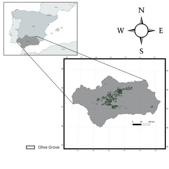
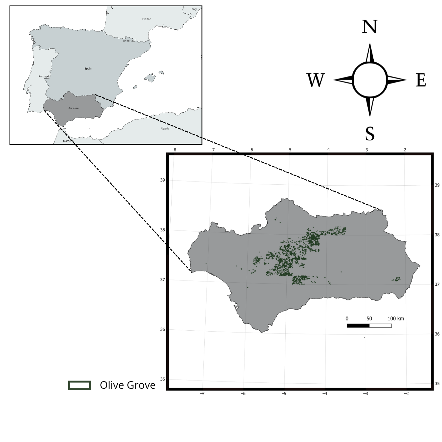
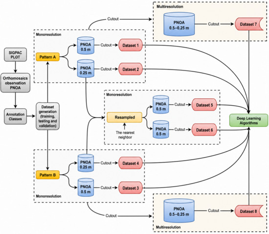
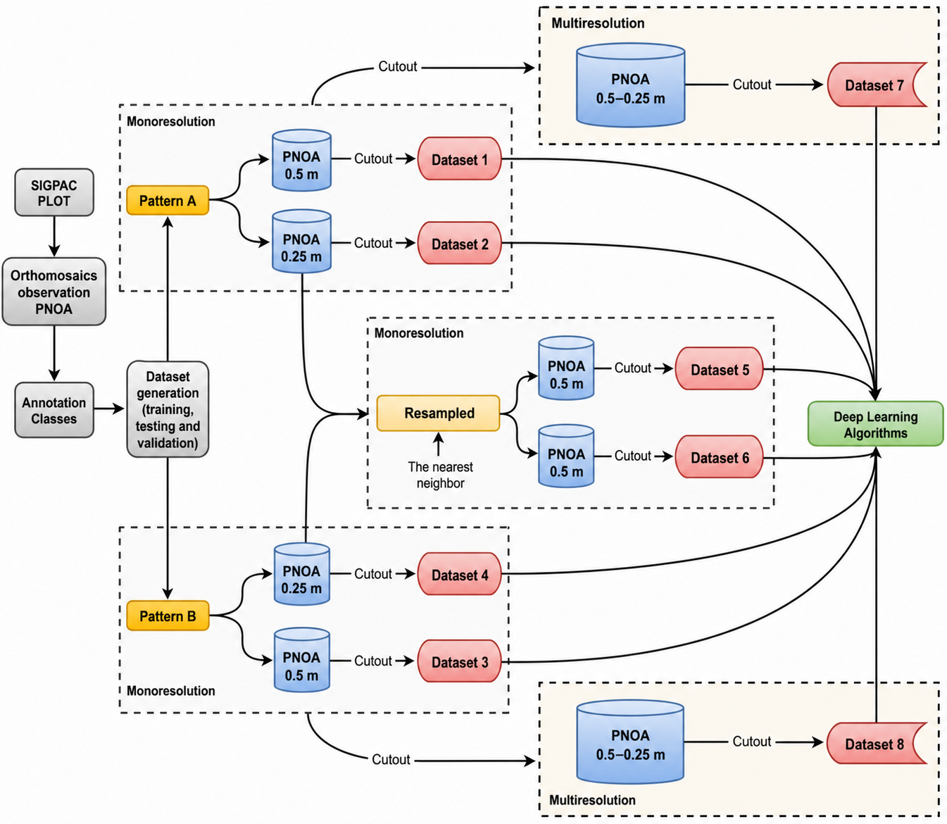
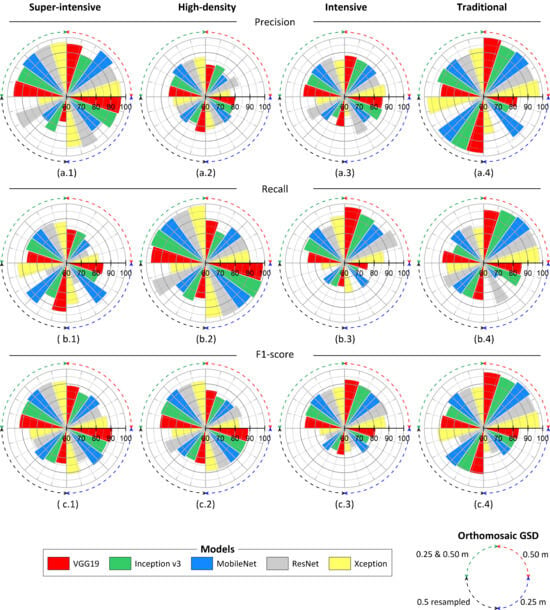
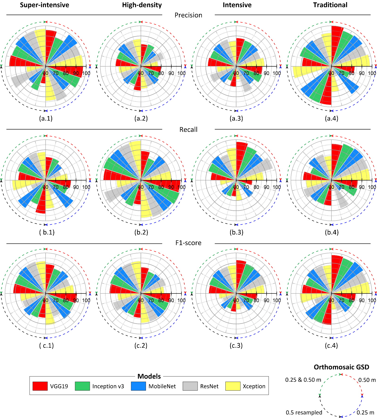
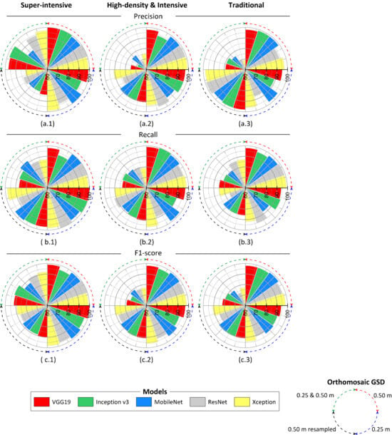
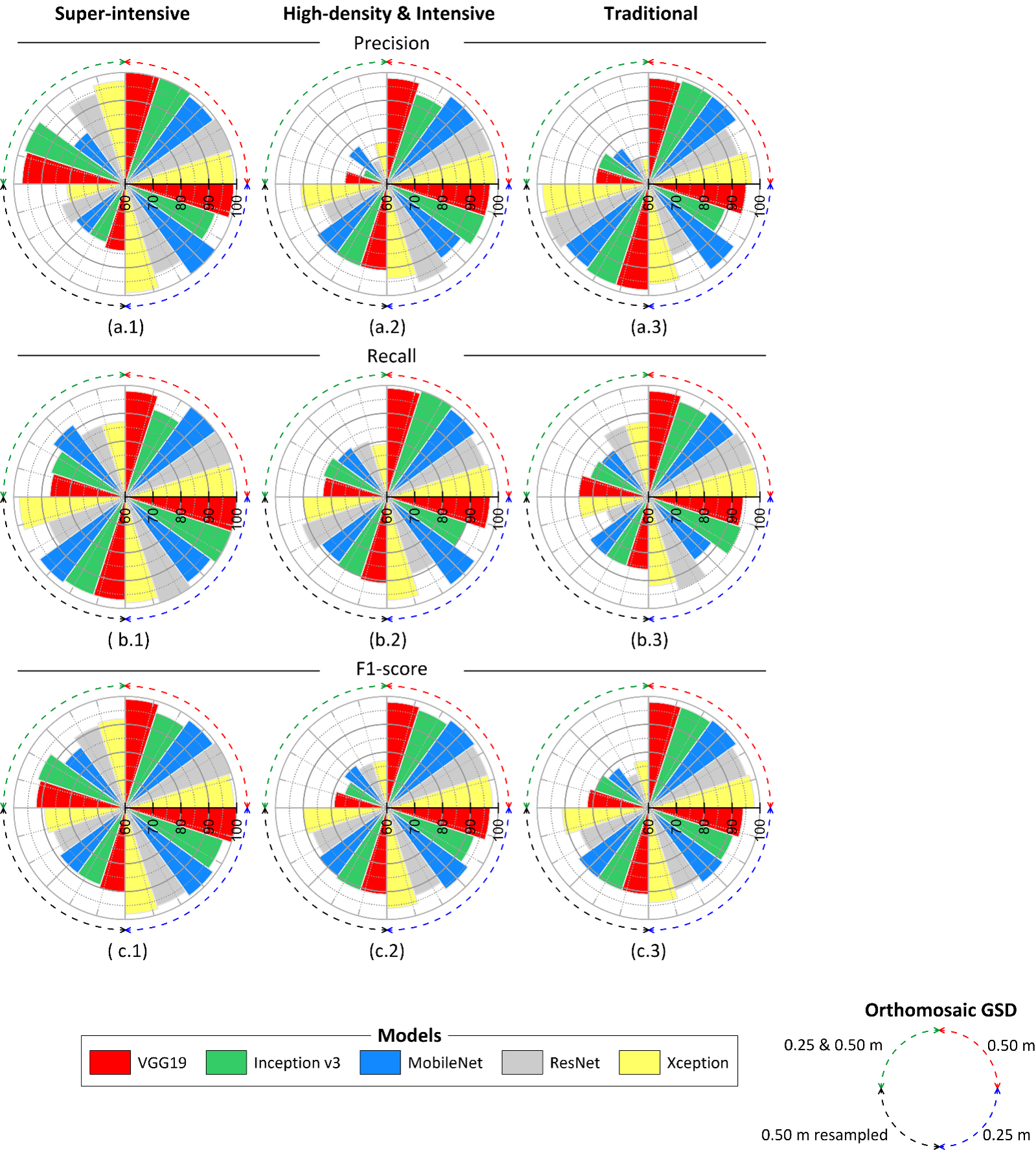

Disclaimer/Publisher’s Note: The statements, opinions and data contained in all publications are solely those of the individual author(s) and contributor(s) and not of MDPI and/or the editor(s). MDPI and/or the editor(s) disclaim responsibility for any injury to people or property resulting from any ideas, methods, instructions or products referred to in the content. |
© 2026 by the authors. Licensee MDPI, Basel, Switzerland. This article is an open access article distributed under the terms and conditions of the Creative Commons Attribution (CC BY) license.