Where Do Crystal Graph Networks Fail? A Space-Group-Resolved Error Analysis of Band Gap Prediction with a Simple Edge-Aware GNN: Crystal-X

Abstract

Graph neural networks (GNNs) for crystal property prediction are typically evaluated by a single aggregate error, which can mask where, and for which classes of materials, these models fail. In this study, we present a space-group-, centering-type-, and band gap-resolved error analysis of GNN band gap prediction on the Materials Project dataset. As a channel for this analysis we use Crystal-X, a deliberately simple model: a standard graph convolutional backbone with two minor architectural modifications, an asymmetric edge convolution and a neighbor-feature transformation, that supplement bond information often treated as secondary in node-centric models. Crystal-X is not a state-of-the-art model: it reaches a band gap MAE of 0.256 eV on the MP 2018.6 dataset, behind ALIGNN (0.22 eV) and PotNet (0.20 eV), though ahead of older baselines such as CGCNN (0.39 eV), SchNet (0.415 eV), and MEGNet (0.33 eV) while using only the nine-property CGCNN atomic feature set. Its value here is as a controlled, low-complexity testbed for the error analysis. That analysis reveals systematic patterns that aggregate MAE conceals: errors concentrate in underrepresented band gap ranges and in low-symmetry and non-centrosymmetric space groups; per-group errors for sparsely populated space groups are dominated by sampling noise; and modest, as-yet-unverified gains from edge-aware convolutions appear in monoclinic and non-primitive-centered systems. We argue that this kind of granular, symmetry-resolved evaluation should accompany aggregate benchmarks when assessing crystal GNNs.

1. Introduction

Materials discovery and prediction with machine learning (ML) methods are positioned to accelerate the development of technologically useful materials. For example, ML models achieved remarkable success in diverse applications ranging from predicting protein structures [1] and earthquake detection [2]. In materials science, graph neural networks (GNNs) have emerged as powerful tools that leverage graph-based representations of atomic structures. By intuitively modeling a lattice structure as a 3D graph, GNNs attempt to simulate the crystal properties as they exist in nature [3].

In 2018, researchers developed a Crystal Graph Convolutional Neural Network (CGCNN) to predict material properties [4]. This model established a paradigm for representing crystals as undirected graphs $G=(V,E)$ with atom features ${\mathbf{v}}_i\in V$ and bond features ${\mathbf{e}}_{ij}\in E$. Numerous models have since been released that aim to predict material properties. This includes SchNet [5], MegNET [6], and Atomistic Line Graph Neural Network (ALIGNN) [7]. ALIGNN model proposed integrated bond angles into the feature vectors by employing the radial basis function (RBF) to encode bond angle information. In all of the aforementioned ideas, there has been one persistent theme: these approaches predominantly focused on node-centric feature learning, treating edge attributes as static secondary parameters despite the critical importance of chemical bonds [8]. In the application of ML in this aspect, Lin et al. have demonstrated improved results with interatomic potential modeling [9].

The recent success of multi-modal models that merge atomic environments, bond features, and auxiliary descriptors boosts accuracy and understanding of complex structures, for example, Moro et al. reduced MAE from 0.50 eV (CGCNN) to 0.40 eV by integrating latent-space similarities with density of states (DOS) [10].

Against this backdrop, the primary contribution of this work is not a new state-of-the-art model but a granular error analysis of GNN band gap prediction: we break test errors down by space group, crystal centering type, and band gap range, and examine how dataset imbalance in the Materials Project propagates into systematic, structure-dependent prediction errors. Such symmetry-resolved diagnostics are, in our experience, rarely reported alongside the customary aggregate MAE, yet they reveal failure modes, underrepresented band gap classes, low-symmetry and non-centrosymmetric groups, and sparsely populated groups whose per-group errors are dominated by sampling noise, that an aggregate number cannot.

As an instrument for this analysis we use Crystal-X, a deliberately simple GNN. Its architectural departures from a standard crystal-graph backbone are minor: an asymmetric edge convolution adapted from the EdgeConv design of Dynamic Graph CNN for point clouds [11], and a neighbor-feature transformation that lifts interatomic-distance encodings into the node feature space. We make no claim of architectural novelty beyond this adaptation. Its simplicity is, for our purposes, a feature: a small model with a compact nine-property atomic feature set makes it easier to attribute error patterns to data and symmetry effects rather than to elaborate architectural machinery, and it provides a clean baseline against which the effect of explicit edge information can be probed via ablation.

2. Methodology

2.1. Graph Embeddings

For crystal embedding, we construct a periodic graph. For each crystal, the atom features are stacked in the array $\mathbf{X}=\{{\mathbf{x}}_1,{\mathbf{x}}_2,\dots ,{\mathbf{x}}_n\}\in {\mathbb{R}}^d$, where d is the dimensionality of the atomic features. Corresponding to each atom feature ${\mathbf{x}}_i$, we define its local environment in terms of its k nearest neighbors. The selection of $k=15$ nearest neighbors balances performance and efficiency. Experiments showed that higher k values produced minimal improvements (<0.02 eV MAE improvement for each successive addition of 5 neighbors) while increasing training time by over 200%. This neighbor feature vector is represented as $\mathcal{N}\left(i\right)=\{{\mathbf{x}}_{v_1},{\mathbf{x}}_{v_2},\dots ,{\mathbf{x}}_{v_k}\}\in {\mathbb{R}}^{k\times d_e}$. Here, $d_e$ is the dimension of each neighbor feature, depending on the number of Gaussian basis functions used to expand each interatomic distance, defined by the discrete steps from $d_{min}$ to $d_{max}$ (with $d_{min}=0$ Å, $d_{max}=20$ Å, step 0.2 Å, giving $d_e=100$). Next, each of the feature $\mathcal{N}\left(i\right)$ is stacked together to form the vector ${\mathbf{X}}_{\mathcal{N}}=\{\mathcal{N}\left({\mathbf{x}}_1\right),\mathcal{N}\left({\mathbf{x}}_2\right),\dots ,\mathcal{N}\left({\mathbf{x}}_n\right)\}$. With this, the first dimension of $\mathbf{X}$ and ${\mathbf{X}}_{\mathcal{N}}$ matches.

In addition to the feature vectors defined above, we employ a third vector defining graph connectivity, $\mathbf{E}\in {\mathbb{R}}^{2\times (N·K)}$. The first row includes the source nodes, while the second row includes the target nodes.

Each node feature, ${\mathbf{x}}_{\mathbf{i}}$, embeds the local property of the element. For this research, we adapted the same atomic feature set proposed in the CGCNN [4], embedding nine properties: group number, period number, electronegativity, covalent radius, valence electrons, 1st ionization energy, electron affinity, orbital block, and atomic volume. For the construction of the neighbor feature ${\mathbf{X}}_{\mathcal{N}}$, we set the $d_{min}=0$ Å and $d_{max}=20$ Å with a step of 0.2 Å.

2.2. Crystal-X Architecture

The Crystal-X architecture consists of two major components: the neighbor feature transformation, characterized by $f_e$, and an asymmetric graph edge convolution function. The algorithm is described in Algorithm 1.

Algorithm 1 Graph Convolution with Edge Features

Input: Node features ${\mathbf{X}}^{\left(l\right)}\in {\mathbb{R}}^{N\times d}$, neighbor features ${\mathbf{X}}_{\mathcal{N}}\in {\mathbb{R}}^{N\times K\times d_e}$, edge connectivity $\mathbf{E}\in {\mathbb{R}}^{2\times (N·K)}$ Parameter: Edge MLP $f_e$, Graph convolution function $f_g$ Output: Updated node features ${\mathbf{X}}^{(l+1)}\in {\mathbb{R}}^{N\times d}$  1: Transform neighbor features: ${\mathbf{X}}_{\mathcal{N}}^{\prime }\leftarrow f_e\left({\mathbf{X}}_{\mathcal{N}}\right)$ {Shape: $N\times K\times d$}  2: Flatten edge features: $\mathbf{e}\leftarrow \mathrm{flatten}\left({\mathbf{X}}_{\mathcal{N}}^{\prime }\right)$ {Shape: $(N·K)\times d$}  3: Initialize: ${\mathbf{H}}_{src}\leftarrow {\mathbf{0}}^{N\times d}$, ${\mathbf{H}}_{tgt}\leftarrow {\mathbf{0}}^{N\times d}$  4: Aggregate edge features to source nodes: ${\mathbf{H}}_{src}\left[i\right]\leftarrow {\sum }_{k:\mathbf{E}[1,k]=i}\mathbf{e}\left[k\right]$ for all $i=1,\dots ,N$  5: Aggregate edge features to target nodes: ${\mathbf{H}}_{tgt}\left[j\right]\leftarrow {\sum }_{k:\mathbf{E}[2,k]=j}\mathbf{e}\left[k\right]$ for all $j=1,\dots ,N$  6: Combine features: ${\mathbf{H}}_{com}\leftarrow {\mathbf{H}}_{src}+{\mathbf{H}}_{tgt}$  7: Apply graph convolution: ${\mathbf{X}}_{conv}\leftarrow f_g({\mathbf{H}}_{com},{\mathbf{X}}^{\left(l\right)},\mathbf{E})$  8: Add residual: ${\mathbf{X}}^{(l+1)}\leftarrow {\mathbf{X}}_{conv}+{\mathbf{H}}_{com}$  9: return  ${\mathbf{X}}^{(l+1)}$

The MLP transformation $f_e$ processes each neighbor feature independently, producing ${\mathbf{X}}_{\mathcal{N}}^{\prime }\in {\mathbb{R}}^{N\times k\times d}$ where d matches the dimensionality of the node feature. Next, this 3D tensor is flattened into a 2D tensor with the shape ${\mathbb{R}}^{(N·k)\times d}$. In order to map this transformed feature vector to our original dimensions of atom feature vector, $\mathbf{X}$, we generate two new tensors, ${\mathbf{H}}_{src}\mathrm{and}{\mathbf{H}}_{tgt}$. The content of these tensors are filled using scatter-and-sum aggregation function. For example, if $\mathbf{E}\left[1\right]=[1,1,2]$, then:

• ${\mathbf{H}}_{src}\left[1\right]+=\mathbf{e}\left[1\right]+\mathbf{e}\left[2\right]$ (edges 1,2 have source node 1)
• ${\mathbf{H}}_{src}\left[2\right]+=\mathbf{e}\left[3\right]$ (edge 3 has source node 2)

In addition to the above, a separate ${\mathbf{H}}_{src}\mathrm{and}{\mathbf{H}}_{tgt}$ helps to retain the bidirectionality of the bond information encoded in the original neighbor feature vector. Finally, for our main edge convolution function, $f_g({\mathbf{H}}_{com},{\mathbf{X}}^{\left(l\right)})$, we propose the following equation for the asymmetric edge convolution layer:

$${\mathbf{X}}_{conv}=f_g\left(\left[{\mathbf{H}}_{com}\parallel {\mathbf{H}}_{com}-{\mathbf{X}}^{\left(l\right)}\right]\right),$$

(1)

where ‖ denotes the concatenation between the aggregated learned neighbor characteristic ${\mathbf{H}}_{com}$ and the node characteristic ${\mathbf{X}}^{\left(l\right)}$, and $f_g$ represents the convolution parameters. A mean aggregator function is embedded in the final step of this layer.

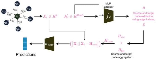
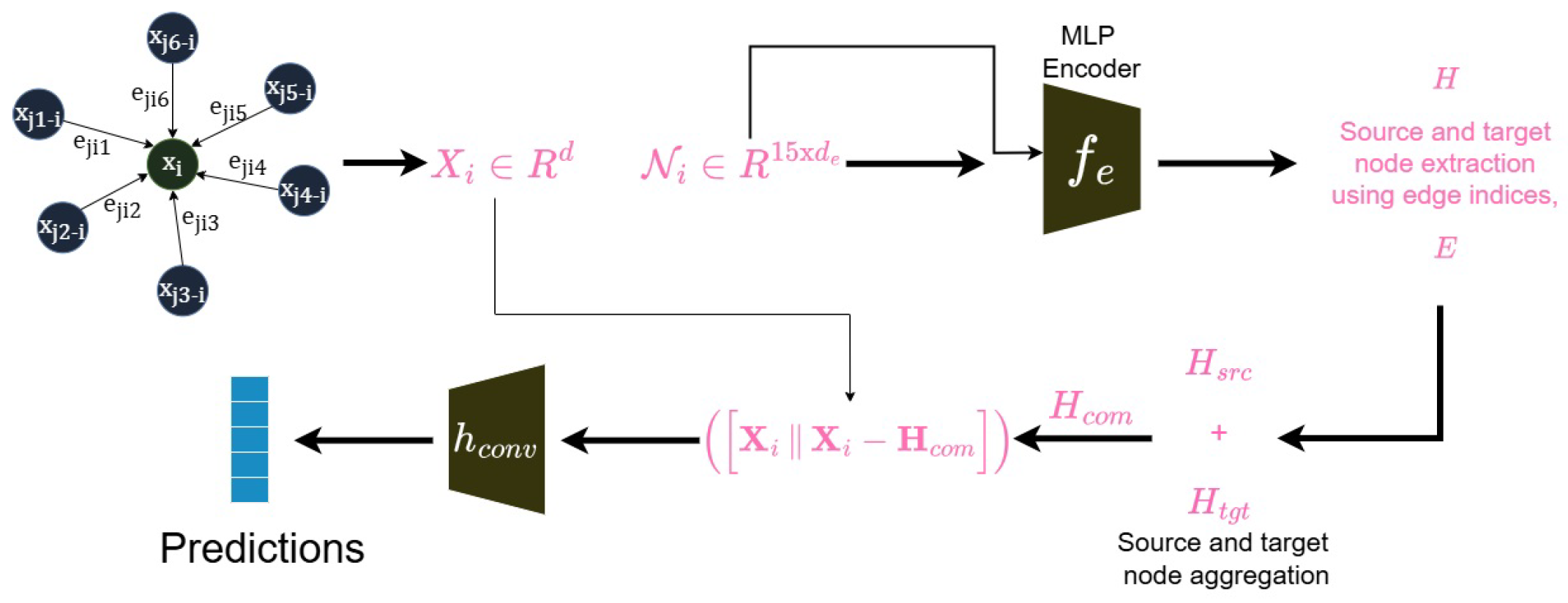
The difference vector in the above function models the local geometry of the crystal relative to the central atom, and by concatenating both the atom features and the edge features, we fulfill our goal of executing a combined node and edge-centric convolution. The overall layout of the model is shown in Figure 1.

Figure 1. Hierarchical message-passing framework combining node features (${\mathbf{x}}_i$) and neighbor/edge features ($\mathcal{N}\left(i\right)$).

The model uses an atom feature length of 64 and 6 convolutional layers. The parameters of $f_e$ are modeled by 3 layers of MLP with SeLU activation functions. In addition, our edge MLP employs hidden dimensions of 128 and 256 and uses a dropout ratio of 0.1. The dataset was split using an 80%:10%:10% ratio for training, validating, and testing.

For training, we implemented the Mean Squared Error (MSE) loss. The model parameters were optimized using the AdamW optimizer with a learning rate of $1\times {10}^{-4}$ and a weight decay of $1\times {10}^{-5}$.

3. Results and Discussion

3.1. Model Performance

Dataset selection critically influences model performance, requiring a rigorous evaluation to mitigate inherent biases, such as skewed class distributions, that may compromise generalization or introduce unintended artifacts. For Crystal-X training, the Materials Project Dataset [12] was chosen, specifically their MP 2018.6 Dataset version, containing 68,580 different inorganic materials, and for general purpose benchmarking, the Matbench Dataset [13] was chosen. The former was selected to evaluate and report the Crystal-X’s performance against current published models and data collected from literature, while the latter was chosen due to its out-of-distribution (OOD) testing strategy. Matbench provides two different datasets for training and testing. The training dataset is constructed using datasets discussed in literature, predominantly the Materials Project dataset. Matbench v0.1 evaluates each task with a fixed nested five-fold cross-validation protocol, so that reported errors reflect performance under a held-out, distribution-shifted split rather than a single random partition. In addition, subsequent results discussed in the Analysis section below are derived from the model trained on the newer MP 2022 Dataset version, containing over 153,000 materials, almost twice the original 2018.6 version. Because the headline comparison in Table 1 uses MP 2018.6 while the per-space-group analysis uses MP 2022, the two should not be read as directly comparable.

Table 1. Comparison of band gap ($E_g$) predictions across different models for the MP 2018.6 Dataset, and scaled error on the Matbench v0.1 benchmark. The underlined and bold values distinguish our results from those of the other models.

Model	Matbench Error	Band-Gap MAE (eV)
CGCNN [4]	0.229	0.39
CrabNet [14]	0.200	0.263
SchNet [5]	0.177	0.415
MEGNet [6]	—	0.33
MODNet [15]	0.165	—
Crystal-X (Ours)	0.162	0.256
ALIGNN [7]	0.140	0.22
PotNet [9]	—	0.20

A regression model was employed to evaluate performance, and the final errors are reported in terms of mean absolute error (MAE) for the MP 2018.6 Dataset, while the Matbench results are reported using the standard scaled error (the lower the better), defined as the ratio of the MAE to the mean absolute deviation (MAD) of the target:

$$\mathrm{Scaled}\mathrm{Error}={\displaystyle \frac{\mathrm{MAE}}{\mathrm{MAD}}}={\displaystyle \frac{{\sum }_{i=1}^n\left|y_i^{\mathrm{pred}}-y_i^{\mathrm{actual}}\right|}{{\sum }_{i=1}^n\left|y_i^{\mathrm{actual}}-{\overline{y}}^{\mathrm{actual}}\right|}}$$

(2)

The model performance, alongside those reported by other GNN regression models for predicting band gaps, is summarized in Table 1. We stress that this table is provided to situate the testbed, not to claim a leaderboard position: Crystal-X does not reach the accuracy of ALIGNN (0.22 eV) or PotNet (0.20 eV) on $E_g$, and the baseline figures are quoted from the literature on potentially different splits, so the comparison is indicative only. For the parameter count and training time per epoch at matched batch size, Crystal-X’s performance is reported with ∼1.002 million parameters and 8.3 s/epoch, ALIGNN’s with ∼4.026 million and 205 s/epoch, and PotNet’s with ∼1.76 million and 26.33 s/epoch. This highlights the architectural simplicity and training speed of Crystal-X while keeping up with these state-of-the-art models’ accuracies.

However, a consistent test dataset is used for reporting the scaled error for all the models for Matbench only, and hence gives a clearer picture about the relative performances of the models. Within those limits, Crystal-X performs reasonably for its size, with a lower reported MAE than the older CGCNN (0.39 eV), SchNet (0.415 eV), and MEGNet (0.33 eV) baselines relative to the original CGCNN implementation on the MP 2018.6 Dataset, this corresponds to a nominal reduction from 0.39 eV to 0.256 eV (34.4%).

It is crucial to emphasize that all models in the Table 1 were trained on Materials Project DFT-calculated band gaps, which inherit the systematic errors from the functional band gap underestimation [16].

3.2. Model Analysis

Recent advancements in ML have underscored the critical need for explainable AI (XAI) in scientific discovery [17]. Traditionally, AI analyses have prioritized predictive accuracy, often treating ML models as black boxes provided they delivered superior results [18]. However, the growing emphasis on trust, reproducibility, and actionable insights has significantly increased the demand for XAI in scientific contexts [19]. Specifically, in materials science, Oviedo et al. highlight two crucial aspects: intrinsic explainability (innately interpretable model architectures) and posthoc analyses (retrospective methods to interpret learned patterns) [20]. Drawing on this framework, we assess Crystal-X qualitatively: its edge-aware design lends a degree of architectural transparency (an intrinsic aspect), and we use posthoc error diagnostics across space groups and band gap ranges to interpret where and why the model fails. We do not claim a full feature-attribution (e.g., SHAP) study here; that is left to future work.

3.2.1. Architectural Rationale of the Testbed Model

Crystal-X’s explicit modeling of edge relationships (e.g., local atomic environments) is a modest design choice rather than a claimed advantage over the field. While CGCNN learns from node-based convolutions that simply join the atom and neighbor features, Crystal-X performs joint edge-node convolutions, directly incorporating pairwise interactions that domain intuition suggests matter for atomic properties. A practical consequence is that the model operates without stacking additional hand-engineered features, such as thermal-stability data: several second-generation models use the Matminer [21] featurizer, which returns up to 128 structural features, whereas ours embeds only nine atomic properties. This compactness is what makes the model a convenient diagnostic testbed, though it also plausibly contributes to its gap relative to PotNet, whereas Crystal-X uses same features and the featurizer algorithm as ALIGNN and CGCNN, making the difference between the latter 3 only on an architectural level.

To probe the effect of the edge-feature processing, we implement a baseline model that runs without it, i.e., concatenating raw neighbor features directly onto our atom feature vector. This experiment on the MP Dataset yielded an average MAE of 0.315 eV, versus an average of 0.256 eV with edge-feature processing across three different seeds. This provides suggestive evidence that explicit treatment of neighbor feature vectors is worth further attention.

3.2.2. Posthoc Analysis: Uncovering Dataset Biases

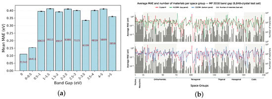
One of the key uses of posthoc analysis is to diagnose systematic limitations in the data or model. The MP dataset used for training exhibits an inherent bias. Figure 2a demonstrates the number of materials per division of the band gap range.

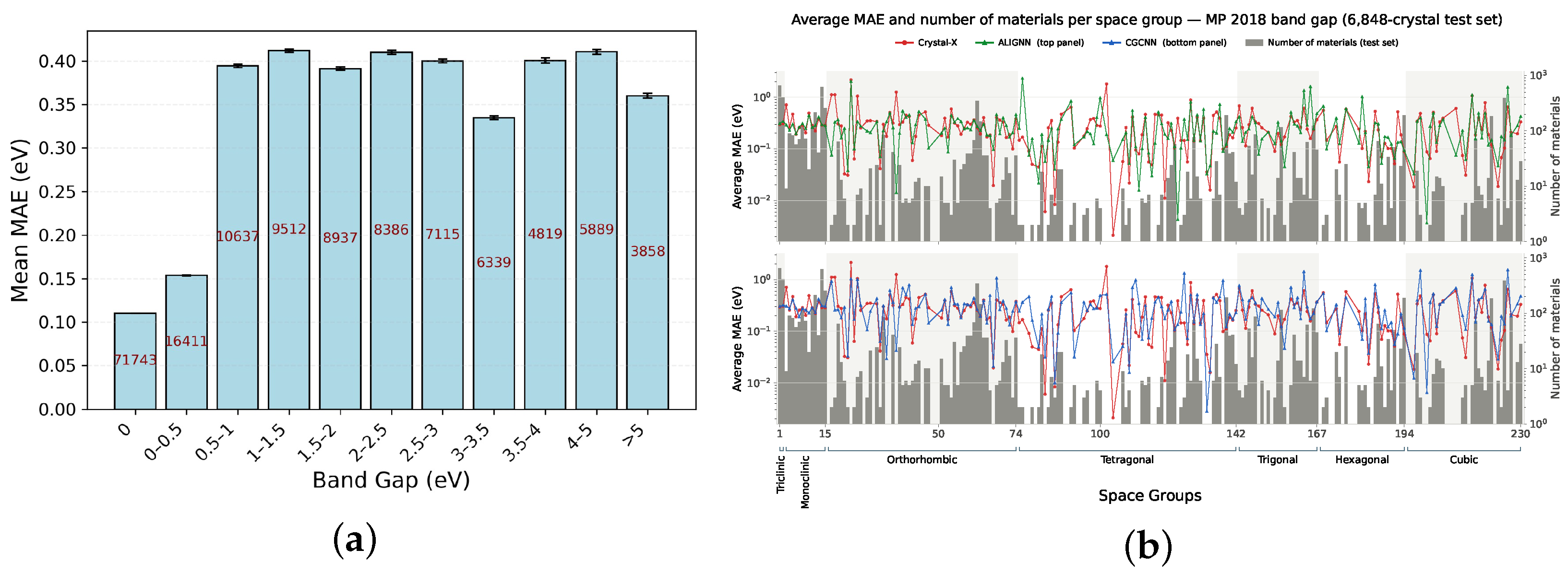
Figure 2. (a) Average MAE, shown by blue bars, and number of materials, shown by red labels on the bars, for band gap ranges on the MP 2022 Dataset. The counts were obtained by comparing the target values of each crystal from the dataset, and then placing them in each band gap bracket. (b) The average MAE and material count for each space group for ALIGNN, Crystal-X, and CGCNN on the MP 2018.6 Dataset. On the left y-axis, we report the MAE for each space group, while the right y-axis shows the material count. The reported analysis is with a consistent testing dataset.

Figure 2a shows low MAE ($0.11$ eV) for metallic materials ($E_g=0$) and MAE ($0.15$ eV) for small-gap materials ($E_g<0.5$ eV), but higher MAE ($0.39$ eV) for larger-gap materials ($E_g>0.5$ eV), reflecting increased complex bonding environments, structural diversity, and less data representation in training sets [22,23]. This highlights the need for targeted strategies like dataset augmentation [24] or SHAP analysis [4,20,25] to enhance prediction accuracy for large band gap materials. We propose a more granular evaluation approach.

We segment our test data based on space group numbers to analyze categories further. Figure 2b shows the relative performance of Crystal-X vs. CGCNN and ALIGNN models. For the graph of Crystal-X vs. CGCNN, the trends exhibit similar error spikes. For the orthorhombic range (50–70 space groups) both models follow almost equivalently low errors. However, for regions with higher asymmetry, such as the monoclinic lattice region (3–15), Crystal-X achieves marginally lower errors.

For centering types, primitive, face-centered, body-centered, and base-centered, Crystal-X also shows lower errors than CGCNN as structural complexity increases. For example:

• Primitive triclinic: Crystal-X records an MAE of 0.30 eV, compared to CGCNN’s 0.42 eV
• Base-centered monoclinic: Crystal-X records 0.31 eV versus CGCNN’s 0.38 eV
• Body-centered tetragonal: Crystal-X records 0.20 eV versus CGCNN’s 0.23 eV

These observations strengthen the hypothesis that modeling explicit edge features improves prediction accuracy in structurally complex settings. In general, Figure 2b shows that, except for some anomalies, the trend stays quite consistent across space groups. For a more comprehensive breakdown of space group analysis, we test Crystal-X’s performance on a broader and more recent dataset, the MP 2022 dataset.

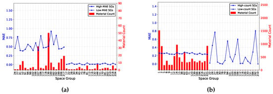
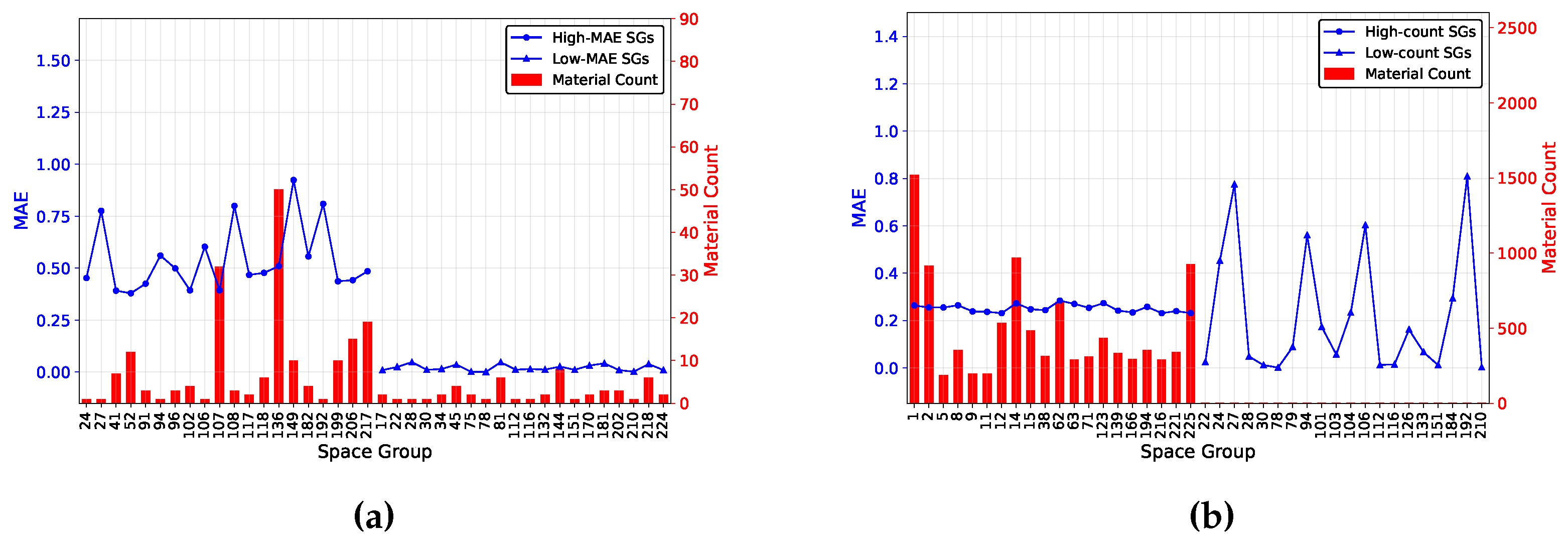
Figure 3a,b represent the standalone data for Crystal-X performance in extreme cases to better understand the limitations of ML models in predicting material properties. In Figure 3a, we display the model performance in the 20 space groups with the highest MAE and the lowest MAE respectively. Similarly, in Figure 3b, we display the model performance in the 20 space groups with the highest number of materials and the lowest number of materials, respectively. Some key findings from this analysis are summarized below:

Figure 3. MAE and material count analysis for selected space groups on the MP 2022 Dataset. (a) MAE and material counts for the 20 space groups with the highest and lowest errors on the MP 2022 Dataset, highlighting the influence of lattice type on model accuracy and explainability. (b) MAE and material counts for the 20 space groups with the highest and lowest counts on the MP 2022 Dataset.

• For triclinic lattice types (Space Groups 1, 2) (MAE ∼0.25 eV), while abundant in the dataset (>15% of samples), the model fails to perform better than the average MAE of the whole dataset. Despite showing comparative improvements, a likely reason for this still remains the model’s failure to capture asymmetric bond angles critical to crystal stability and material properties. An improvement to address this may include explicit encoding of bond angle information, as was originally proposed by ALIGNN [7]. This will help us improve the model’s overall generalizability to any irregularly structured crystal systems.
• Non-centrosymmetric systems, particularly in the orthorhombic (space groups 25, 46), tetragonal (space group 102, 106), and hexagonal lattice (space group 182) types, exhibit high prediction errors, along with also being relatively rare. This suggests that the model’s poor performance can be accounted for by both data scarcity and its inability to capture structural features of non-centrosymmetric systems.
• Figure 3a shows the materials with the lowest MAE for several crystal systems on the right side (e.g., space groups 22, 28, 112, 151, etc.) also happen to be the ones with extremely low counts (<5 samples). While on the left side, enantiomorphic cubic variants (e.g., Space Group 206) show high errors (MAE ∼0.45 eV) despite a simple crystal structure. We suggest that the model obtains the lowest MAE because of shared crystallographic features with the trained materials. These per-group MAEs are computed on fewer than five test structures and are therefore dominated by sampling noise; we treat them as anecdotal rather than as evidence of a systematic effect.

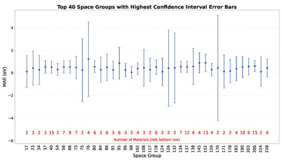
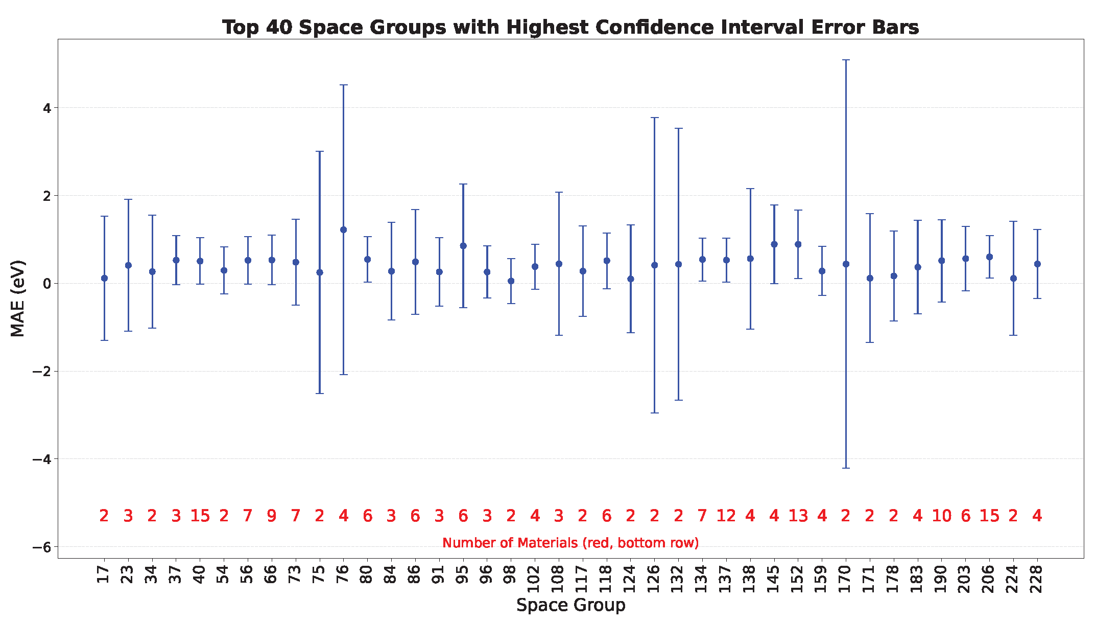
To test these examples, we used 95% confidence interval tests for 40 space groups with the longest error bars. We note that for groups with very small n (some with $n<5$), the t-interval assumptions are weak and the resulting intervals are only loosely indicative. The confidence intervals quantify the uncertainty in the estimated mean MAE for each space group. A longer confidence interval error bar for a certain space group would reflect that the model is less certain about the exact value of MAE. The formula used for calculating the 95% confidence interval is as follows:

$$CI=\overline{X}\pm t_{{\displaystyle \frac{\alpha }{2}},df}\times {\displaystyle \frac{\sigma }{\sqrt{n}}}$$

where $\overline{X}$ is the sample mean, $t_{\alpha /2,df}$ is the critical value of the t-distribution at the desired confidence level (95%) with degrees of freedom $df=n-1$, $\sigma$ is the sample standard deviation, and n is the sample size. The difference between the upper and lower value is equal to the length of error bars.

The Figure 4 shows MAE for the most uncertain predictions. For example, space groups 17, 98, 124, and 171, exhibit MAE in the range of 0.1 eV, but their high confidence interval error bar range indicates that the model is actually less certain in these groups due to low count.

Figure 4. Per-space-group mean MAE (blue points) with 95% confidence intervals (blue bars) for the 40 space groups with the widest intervals on the MP 2022 test set. The red numbers along the bottom row give the number of test materials in each group; the widest intervals correspond to the smallest counts. Owing to the very small per-group sample sizes, some intervals extend below zero; the MAE itself is non-negative.

Figures like Figure 2 and Figure 4 are often skipped out of model analysis. As such, this hinders the overall generalizability and interpretability of the model. In order for machine learning to improve its material discovery capabilities, a more in-depth benchmarking protocol and dataset imbalances need to be discussed for every model.

To improve model performance in areas where we lack data, we suggest developing better feature selection algorithms that result in better learning. For example, researchers have proposed an entropy-targeted active learning (ET-AL) framework designed to strategically select new data points that enhance representations of underrepresented crystal systems [24]. This technique has been particularly effective in enhancing model generalizability and improving accuracy in accelerated materials discovery pipelines.

In addition, Gong et al. proposed simple hybridization of GNNs and descriptors [26]. Instead of developing complex GNN architectures to improve accuracy, a concatenation of the descriptor vector with the learned features vector has shown improvements in learning from limited data points over pure GNN architectures such as CGCNN.

Taken together, these diagnostics answer the question where GNNs fail to capture crystal symmetry: they fail predominantly on large-gap materials ($E_g$ > 0.5 eV, versus near-metallic gaps where error is lowest), on low-symmetry space groups (triclinic and monoclinic), and on non-centrosymmetric systems: regions that are, with few exceptions, also underrepresented or structurally difficult in the training data. The other angle, why these models fail in these regions, is left for future work for a more intrinsic exploration of the failure modes.

4. Conclusions

The central message of this work is methodological: aggregate benchmark numbers (e.g., MAE) hide systematic structure in where a model’s errors actually fall. Our space-group-, centering-, and band gap-resolved error analysis on the Materials Project dataset shows that prediction errors concentrate systematically in underrepresented band gap classes and in low-symmetry and non-centrosymmetric space groups, that class imbalance propagates directly into model errors, and that per-group statistics for sparsely populated space groups are dominated by sampling noise and should be interpreted with care. We answer this question by breaking down the failure modes of the models: localizing failure by space group, centering type, and band gap range. To demonstrate this analysis, we used Crystal-X, a simple GNN whose two minor modifications to a standard backbone, a neighbor-feature transformation and an asymmetric edge convolution, make it a compact, controlled testbed; it reaches a reasonable 0.256 eV band gap MAE with only nine atomic features, but it does not match state-of-the-art models such as ALIGNN or PotNet, and we do not present it as a competitor to them. The apparent gains from edge-aware convolutions in monoclinic and non-primitive-centered systems are encouraging. We hope this kind of granular, symmetry-resolved error reporting becomes a routine companion to aggregate metrics in crystal-property ML, and we see targeted data acquisition for underrepresented symmetry classes, e.g., via entropy-targeted active learning, as the most promising next step.

References

- Senior, A.W.; Evans, R.; Jumper, J.; Kirkpatrick, J.; Sifre, L.; Green, T.; Qin, C.; Žídek, A.; Nelson, A.W.R.; Bridgland, A.; et al. Improved protein structure prediction using potentials from deep learning. Nature 2020, 577, 706–710. [Google Scholar] [CrossRef] [Scilit] [PubMed]
- Zhexebay, D.; Skabylov, A.; Ibraimov, M.; Khokhlov, S.; Agishev, A.; Kudaibergenova, G.; Orazakova, A.; Agishev, A. Deep Learning for Early Earthquake Detection: Application of Convolutional Neural Networks for P-Wave Detection. Appl. Sci. 2025, 15, 3864. [Google Scholar] [CrossRef] [Scilit]
- Schütt, K.T.; Arbabzadah, F.; Chmiela, S.; Müller, K.R.; Tkatchenko, A. Quantum-chemical insights from deep tensor neural networks. Nat. Commun. 2017, 8, 13890. [Google Scholar] [CrossRef] [Scilit] [PubMed]
- Xie, T.; Grossman, J.C. Crystal Graph Convolutional Neural Networks for an Accurate and Interpretable Prediction of Material Properties. Phys. Rev. Lett. 2018, 120, 145301. [Google Scholar] [CrossRef] [Scilit] [PubMed]
- Schütt, K.T.; Sauceda, H.E.; Kindermans, P.J.; Tkatchenko, A.; Müller, K.R. SchNet—A deep learning architecture for molecules and materials. J. Chem. Phys. 2018, 148, 241722. [Google Scholar] [CrossRef] [Scilit] [PubMed]
- Chen, C.; Ye, W.; Zuo, Y.; Zheng, C.; Ong, S.P. Graph Networks as a Universal Machine Learning Framework for Molecules and Crystals. Chem. Mater. 2019, 31, 3564–3572. [Google Scholar] [CrossRef] [Scilit]
- Choudhary, K.; DeCost, B. Atomistic Line Graph Neural Network for improved materials property predictions. npj Comput. Mater. 2021, 7, 185. [Google Scholar] [CrossRef] [Scilit]
- Pauling, L. The nature of the chemical bond: Application of results obtained from quantum mechanics and from a theory of paramagnetic susceptibility to the structure of molecules. J. Am. Chem. Soc. 1931, 53, 1367–1400. [Google Scholar] [CrossRef] [Scilit]
- Lin, Y.; Yan, K.; Luo, Y.; Liu, Y.; Qian, X.; Ji, S. Efficient Approximations of Complete Interatomic Potentials for Crystal Property Prediction. In Proceedings of the 40th International Conference on Machine Learning, Honolulu, HI, USA, 23–29 July 2023; Krause, A., Brunskill, E., Cho, K., Engelhardt, B., Sabato, S., Scarlett, J., Eds.; PMLR: Cambridge, MA, USA, 2023; Volume 202, pp. 21260–21287. [Google Scholar]
- Moro, V.; Loh, C.; Dangovski, R.; Ghorashi, A.; Ma, A.; Chen, Z.; Kim, S.; Lu, P.Y.; Christensen, T.; Soljačić, M. Multimodal foundation models for material property prediction and discovery. Newton 2025, 1, 100016. [Google Scholar] [CrossRef] [Scilit]
- Wang, Y.; Sun, Y.; Liu, Z.; Sarma, S.E.; Bronstein, M.M.; Solomon, J.M. Dynamic Graph CNN for Learning on Point Clouds. ACM Trans. Graph. 2019, 38, 146:1–146:12. [Google Scholar] [CrossRef] [Scilit]
- Jain, A.; Ong, S.P.; Hautier, G.; Chen, W.; Richards, W.D.; Dacek, S.; Cholia, S.; Gunter, D.; Skinner, D.; Ceder, G.; et al. Commentary: The Materials Project: A materials genome approach to accelerating materials innovation. APL Mater. 2013, 1, 011002. [Google Scholar] [CrossRef] [Scilit]
- Dunn, A.; Wang, Q.; Ganose, A.M.; Dopp, D.A.; Jain, A. Benchmarking Materials Property Prediction Methods: The Matbench Test Set and Automatminer Reference Algorithm. npj Comput. Mater. 2020, 6, 138. [Google Scholar] [CrossRef] [Scilit]
- Wang, A.Y.T.; Kauwe, S.K.; Murdock, R.J.; Sparks, T.D. Compositionally restricted attention-based network for materials property predictions. npj Comput. Mater. 2021, 7, 77. [Google Scholar] [CrossRef] [Scilit]
- De Breuck, P.P.; Hautier, G.; Rignanese, G.M. Materials property prediction for limited datasets enabled by feature selection and joint learning with MODNet. npj Comput. Mater. 2021, 7, 83. [Google Scholar] [CrossRef] [Scilit]
- Sim, E.; Song, S.; Burke, K. Quantifying Density Errors in DFT. J. Phys. Chem. Lett. 2018, 9, 6385–6392. [Google Scholar] [CrossRef] [Scilit] [PubMed]
- Samek, W.; Montavon, G.; Vedaldi, A.; Hansen, L.K.; Müller, K.R. Explainable AI: Interpreting, Explaining and Visualizing Deep Learning. In Explainable AI: Interpreting, Explaining and Visualizing Deep Learning; Samek, W., Montavon, G., Vedaldi, A., Hansen, L.K., Müller, K.R., Eds.; Lecture Notes in Computer Science; Springer: Cham, Switzerland, 2019; Chapter 1; pp. 5–12. [Google Scholar] [CrossRef] [Scilit]
- Guidotti, R.; Monreale, A.; Ruggieri, S.; Turini, F.; Giannotti, F.; Pedreschi, D. A Survey Of Methods For Explaining Black Box Models. ACM Comput. Surv. 2018, 51, 93:1–93:42. [Google Scholar] [CrossRef] [Scilit]
- Gilpin, L.H.; Bau, D.; Yuan, B.Z.; Bajwa, A.; Specter, M.; Kagal, L. Explaining Explanations: An Overview of Interpretability of Machine Learning. In Proceedings of the 2018 IEEE 5th International Conference on Data Science and Advanced Analytics (DSAA), Turin, Italy, 1–4 October 2018; pp. 80–89. [Google Scholar] [CrossRef] [Scilit]
- Oviedo, F.; Ferres, J.L.; Buonassisi, T.; Butler, K.T. Interpretable and Explainable Machine Learning for Materials Science and Chemistry. Acc. Mater. Res. 2022, 3, 597–607. [Google Scholar] [CrossRef] [Scilit]
- Ward, L.; Dunn, A.; Faghaninia, A.; Zimmermann, N.E.R.; Bajaj, S.; Wang, Q.; Montoya, J.H.; Chen, J.; Bystrom, K.; Dylla, M.; et al. Matminer: An open source toolkit for materials data mining. Comput. Mater. Sci. 2018, 152, 60–69. [Google Scholar] [CrossRef] [Scilit]
- Ward, L.; Agrawal, A.; Choudhary, A.; Wolverton, C. A general-purpose machine learning framework for predicting properties of inorganic materials. npj Comput. Mater. 2016, 2, 16028. [Google Scholar] [CrossRef] [Scilit]
- Meredig, B.; Agrawal, A.; Ong, S.P.; Saal, J.E.; Doak, J.; Thompson, A.; Yang, K.; Choudhary, A.; Wolverton, C. Combinatorial screening for new materials in unconstrained composition space with machine learning. Phys. Rev. B 2014, 89, 094104. [Google Scholar] [CrossRef] [Scilit]
- Zhang, H.; Chen, W.; Rondinelli, J.M.; Chen, W. ET-AL: Entropy-targeted active learning for bias mitigation in materials data. Appl. Phys. Rev. 2023, 10, 021403. [Google Scholar] [CrossRef] [Scilit]
- Lundberg, S.M.; Lee, S.I. A Unified Approach to Interpreting Model Predictions. Adv. Neural Inf. Process. Syst. 2017, 30, 4765–4774. [Google Scholar]
- Gong, S.; Yan, K.; Xie, T.; Shao-Horn, Y.; Gomez-Bombarelli, R.; Ji, S.; Grossman, J.C. Examining graph neural networks for crystal structures: Limitations and opportunities for capturing periodicity. Sci. Adv. 2023, 9, eadi3245. [Google Scholar] [CrossRef] [Scilit] [PubMed]
Disclaimer/Publisher’s Note: The statements, opinions and data contained in all publications are solely those of the individual author(s) and contributor(s) and not of MDPI and/or the editor(s). MDPI and/or the editor(s) disclaim responsibility for any injury to people or property resulting from any ideas, methods, instructions or products referred to in the content. |
© 2026 by the authors. Licensee MDPI, Basel, Switzerland. This article is an open access article distributed under the terms and conditions of the Creative Commons Attribution (CC BY) license.