


Abstract
Here we investigate the topological phase transition of a general one-dimensional (1D) disordered Su–Schrieffer–Heeger (SSH) model, with two tunable parameters, the disorder distribution center and a dimensionless ratio k between the disorder strengths of the intracell and intercell hopping terms. First, for each realization or the ensemble average, we numerically observe a topological phase transition (TPT) with quantized real-space winding number jump and disappearing of zero-energy edge states when the disorder strength increases. Second, surprisingly, we find that the critical point of TPT is determined by the equality between the geometry means of intracell and intercell hopping terms. Third, a new theory based on the redefined sublattices is developed, which proves that the critical condition of TPT of the 1D disordered model is governed by the equality of the products of odd and even hopping terms and agrees with our numerical results. The theory also shows that the sudden change picture of TPT, not the gradual inverse picture, is correct, and that the origin of TPT is from the sub-symmetry of the model. Fourth, other models with different parameters are also studied. The TPTs of these models also follow our theoretical predictions. These results contribute to a better understanding of TPTs in 1D disordered systems.
1. Introduction
Topology is an important concept in modern physics. Among the topological models, the one-dimensional (1D) Su–Schrieffer–Heeger (SSH) model may be the simplest one which can possess the topologically non-trivial band structure [1]. Along with the rapid development of topological models, the extension of the original SSH model is widely investigated, which includes extending the original SSH model to the higher spatial dimensions [2], enlarging the unit cell of the original SSH model [3,4] and introducing more terms into the model, e.g., long-range hoppings [5,6] and spin–orbit coupling.
An interesting research direction for the extended SSH model is introducing disorder into the 1D SSH model. Disorder should be understood as an effective description of static and/or experimentally relevant fluctuations in the hopping amplitudes, which may arise from several physical sources. These include, for instance, structural imperfections, lattice distortions, or fabrication-induced inhomogeneities, as commonly considered in disordered SSH-type systems. Disorder can drive the system from being topologically nontrivial to trivial as the disorder strength increases and vice versa. This disorder-induced topological phase transition (TPT) is found in optical fiber systems [7], atomic chains [8,9,10], mechanical systems [11], waveguides [12], etc. One of essential difficulties for the topological study of disordered systems is to find a topological invariant to signify the TPT. Unlike periodic systems where the topological invariant could be well defined in k-space, for disordered systems, we need to find other topological invariants. For example, the Bott index is proposed to describe the topology of disordered systems [13], which also leads to the birth of real-space Chern number [14]. Recently, real-space winding number [10,15] is proposed and has been widely used to study topology of disordered systems, which is powerful tool since it is defined by the direct eigen-solutions of disordered systems. Also, many new topological phenomena are observed for 1D disordered SSH models, and theories have been constructed to understand these new phenomena. The spring-mass chain with disorder [16] is investigated numerically to find the bilateral capacity of the disorder to drive topological transitions. The SSH model with only disordered intercell hopping terms [11] is studied, where a -topological invariant is defined by the non-Hermitian part of the Hamiltonian, and its fluctuation is also investigated numerically and theoretically. Nava et al. have studied the nonequilibrium current through the disordered SSH chain connected to two baths [12], and the even–odd differential occupancy as the topological invariant is used to describe the topological nontrivial phases. Very recently, the 1D disordered SSH model with a ratio of disorder strength between the intracell and intercell hopping terms was studied by Ren et al. [17]. The gapped and ungapped TAI phases were found, and for the ungapped TAI phase, it was demonstrated that the localized bulk states and topological edge states can coexist stably at zero energy.
However, with all these fruitful studies of topological properties, the critical condition and physical origin of TPT of 1D disordered SSH models has not been well investigated. In other words, questions, such as “Which parameters determine the critical TPT condition of 1D disordered SSH models and can we predict the TPT by these parameters?” and “What’s the correct picture and the origin of TPT of 1D disordered SSH models?” still need to be answered.
In this work, we study a general 1D disordered SSH model with tunable parameters: , which determines the disorder distribution center, and k, which is the dimensionless ratio of disorder strength between the intracell hopping terms and the intercell hopping terms. As each individual realization explicitly preserves chiral symmetry, the ensemble automatically satisfies the corresponding symmetry constraints required in the statistical topological insulators description [18]. So our model can be viewed as a specific subset of STIs. First, a 1D disordered SSH model with and is investigated. We observed edge-state disappearing in the energy spectrum at certain critical point with increasing disorder strength. Also, by numerical calculation, we found that the real-space winding number jumped from the unit to zero in the process, which demonstrates that every realization undergoes TPT. Although the critical point differs for each realization, the critical condition of the TPT for the disordered model can be defined based on the ensemble average of all realizations. Furthermore, we surprisingly found that the critical point of every realization or the critical point of ensemble average was determined by the equality between the geometric means of the intracell and intercell hopping terms. Since we naively thought that the TPT was from the local gradual inverse between the averaged intercell and intracell terms, these interesting results regarding geometric means are anti-intuition and also imply the different origin of the TPT. To explain these phenomena, we develop the theory based on the redefined sublattices and prove that the critical point of TPT is really governed by equality between the product’s intracell and intercell hopping terms. Our theory also reveals that the sudden change picture of TPT is the correct one and the origin of the TPT of disordered 1D SSH model is from the sub-symmetry of the system. Since our theory is a general one for 1D disordered models, it should be also available for disordered SSH models with different and k. Our numerical results demonstrate that our theory is available for other models, including the model in work [17], where two TPTs for TAI phases can be explained by our theory. Our theoretical and numerical results may be useful for exploring the topological study of 1D disordered systems.
This paper is organized as follows. In Section 2, the general 1D disordered SSH model with a certain ratio of disorder strength between the intracell hopping term and the intercell hopping term is introduced, as well as the real-space winding number. In Section 3, we provide a overview of the topological properties and disorder properties of the proposed 1D disordered SSH model, e.g., the finite scale energy spectrum, the edge states, the real-space winding number, its ensemble average, and the different means of the hopping terms. Some puzzling phenomena are revealed. In Section 4, the TPT condition of the 1D disordered SSH model is derived. In Section 5, the general 1D disordered SSH models with other parameters are investigated to verify the TPT condition. Finally, conclusions are given in Section 6.
2. Model and Methods
In this section, we will introduce a general 1D disordered SSH model with two tunable parameters for the topological study as shown in Figure 1. The Hamiltonian of the disordered SSH model is given by
where and are the annihilation and the creation operator corresponding to the sites at the A and the B sublattices of the ith unit cell and , m is the total number of unit cells. The disorder is introduced in following ways. The intracell hopping terms are , and the intercell hopping terms are , where W is the disorder strength, k is the first tunable parameter for the chosen ratio between the disorder strengths for intercell and intracell hopping terms, and are the independent random numbers for site-A and site-B in ith cell with even distribution in the range , and is the second tunable parameter for the distribution center of random numbers. Unless otherwise specified, in this work, we choose , , and , corresponding to the initial periodic system with topologically nontrivial phase in the clean limit.
Figure 1.
SSH model with a certain ratio of disorder strength between the intracell hopping term and the intercell hopping term . The box represents the finite model with N lattices.
We hope to explain more details for the two tunable parameters. First, is introduced in to enhance the universality of the model. With , the random number all take positive values and both distribution centers of and are . We will see that the positive and will greatly increase the numerical stability for our topological study. With between 0 and , the random numbers may take negative values, and the model exhibits some distinct features. With , both distribution centers of and are 0, and our model is same as the model from Ren’s work [17]. Second, the ratio k can tune the relative disorder strength between the intracell terms and the intercell terms and the arithmetic mean values of and . For example, when we choose , the arithmetic mean values of intracell hopping terms and intercell hopping terms are and , respectively. Hence, the size relationship between arithmetic mean values could be changed if k is not unit and W is large enough. According to the traditional topology theory of SSH model, the TPT from topologically nontrivial to trivial or vice versa may appear for our model. The physical realization of the parameter k relies on both the initial design of the system and external-field-controlled tuning.
From the view of symmetries, the disorder on the hopping terms breaks translation symmetry, but the chiral symmetry is preserved for the model of Equation (1), i.e., where is the chiral operator. The chiral symmetry also indicates that, when the model is topologically nontrivial, the zero-energy states may appear for the model with the open boundary condition.
In this paper, we will use the following numerical methods for topological study. For the first one, we solve the Schodinger equation by the Hamiltonian Equation (1) with an open boundary condition. In more detail, we write the Hamiltonian Equation (1) as a matrix. In this work, we choose the total lattice number for the finite model with open boundary condition, so that the Hamiltonian is matrix. Numerically, we use MATLAB R2022B’s Eigs-function to process this eigen-equation, which outputs the eigenvalues and eigenfunctions of the our model with the open boundary condition. The energy spectrum of the system is obtained by rearranging the eigenvalues, and the eigenfunctions corresponding eigenvalues could also be obtained.
Then, based on the results of eigenfunctions, we can obtain the real-space winding number [15] for every realization of our disordered model to signify the topological property of the model. The real-space winding number could be calculated by
where , for or B. The ith column in is the sector of the ith eigenfunctions below the gap under consideration. is the projector operator of sublattice . The position operator is , whose eigenvalues are the center of mass of the Wannier states. We will see that the real-space winding number approach is a good method for the topological study of 1D disordered systems since it can reproduce an exactly quantized winding number for disordered 1D realizations.
The second numerical method is based on the transfer matrix method [19]. To acquire the transmission spectra, we assume that the disordered SSH model is with the incidence from left-side waveguide and the transmission at the right-side waveguide. Then, the wavefunction magnitude on the sites satisfies the matrix equation:
where is the transfer matrix for the nth site, given by , is the energy of incident electrons, is the hopping term from the nth site to the th site no matter it is or , and is the wavefunction magnitude on the nth site. We suppose the disordered model starts from site and ends at . Then, the relation between the transmitted wavefunction at the sites and of the right waveguide and the incident wavefunction at the cites and of the left waveguide can be obtained by
The global transfer matrix can be obtained using the parameters of our model. We assume the transmitted wavefunction to be and at the right waveguide. With Equation (4), we can obtain the wavefunction and at the left waveguide. Since both wavefunction and have the form , the incident-wave amplitude and the reflected-wave amplitude can be obtained from and . So that the transmission coefficient and the reflection coefficient can be obtained. Based on the transfer matrix method, we can calculate the transmission spectra of the realizations and also can check the results of the interface states obtained by the first numerical method.
3. Results for the Model with
In this section, we will study the TPT of our disordered SSH model from several aspects. First, we show the energy spectra of the finite-size disordered SSH model with the open boundary condition and find the clues of TPT, e.g., the zero-energy states which look like topological edge states exist with weak disorder and then disappear when the disorder increases to a very large value. Second, the real-space winding number is calculated, which clearly shows the TPT, since jumps from 1 to 0 when the disorder strength increases [15]. Third, the properties of TPT are also investigated, e.g., the relation between the critical point and the disordered hopping terms.
3.1. Energy Spectrum and Edge States of a Realization
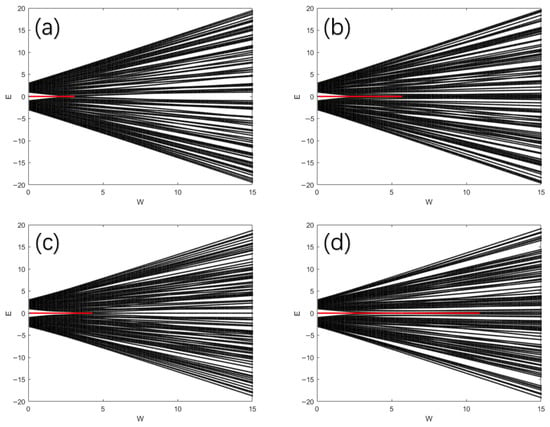
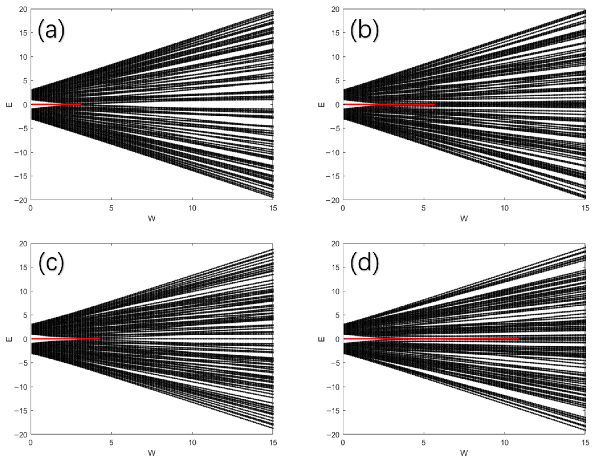
In order to study the topological properties, we calculate the energy spectra versus disorder strength W of four typical finite-size () realizations of our model with open boundary condition. Based on the Hamiltonian of a realization with the certain disorder strength W of our model, we calculate the eigen-functions and eigenvalues. Then, the energy spectrum versus W of the finite-size realization can be obtained. In Figure 2a–d, we show the energy spectra versus W for four disorder realizations.
Figure 2.
The energy spectrum of the finite model with lattice number versus the disorder strength W for different realizations. The red line denotes the topological edge states of our model with the open boundary condition. (a) The 1st realization; (b) The 2nd realization; (c) The 12th realization; (d) The 24th realization.
We observe the following characteristics of the spectra from Figure 2a–d. First, We find that, for the periodic system with (no disorder), two degenerated zero-energy states exist inside the gap since we set the original value of the intercell hopping term to larger than that of the intracell hopping term and the system is topologically nontrivial. Second, under small disorder, the degenerate zero-energy boundary states still exist inside the gap while the gap width decreases with increasing W. Third, when the disorder reaches a certain threshold value for one realization, the gap between two bands will be closed while the zero-energy states are still there. The co-existence of the closed gap and the topological edge-states are also observed in [17,20], and have been called un-gapped TAI in [17]. The zero-energy states disappear with a further increase in W; then, the whole range of the spectrum is occupied by the disordered eigen-values of localized states. This process is obviously different from the traditional TPT with gap closing and reopening for periodic systems, since no gap reopening occurs for larger disorder strengths W. However, these findings with increasing disorder strengths are very inspiring. From the topological nontrivial property with to the disappearance of zero-energy states with a large value of W, we can guess that there may be a TPT in the process, which needs to be further studied carefully.
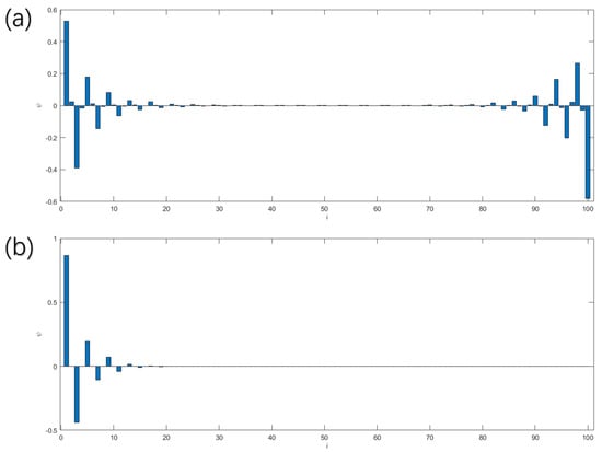
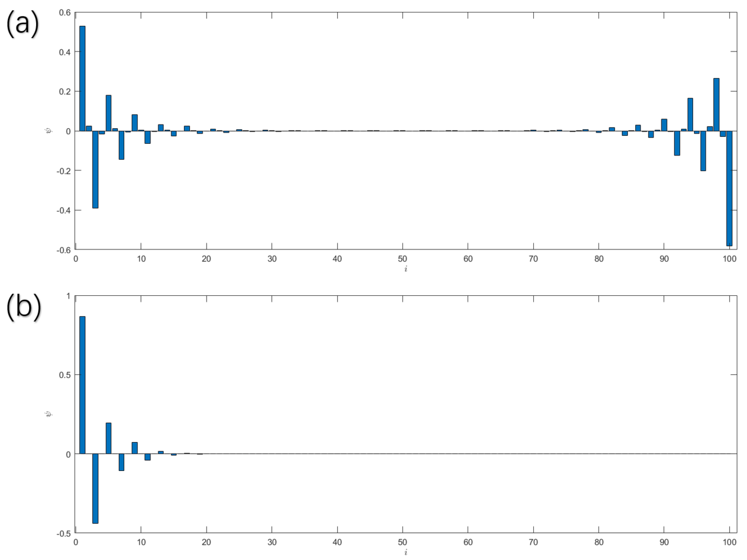
Figure 3a demonstrates the wavefunction of the zero-energy state versus the lattice number i for the realization in Figure 2a with W = 1. Obviously, such a zero-energy state for disordered systems is localized at both left and right boundaries of the finite model with the open boundary condition. We notice that the wavefunction of the zero-energy state in Figure 3a does not strictly satisfy the requirement of chiral symmetry, but the minor error vanishes as the number of lattice sites increases. In contrast, we present a zero-energy state of a much longer model with in Figure 3b, which clearly satisfies the chiral-symmetry requirement. So the minor error is from coupling of the zero-energy states in our model with finite size .
Figure 3.
(a) The wavefunction versus the x of two zero-energy edge-states for the realization of Figure 2a, with total lattice number . The property of chiral symmetry—that the field on one kind sublattices for one edge-state is zero—is not strictly complied, which is caused by the coupling between two edge states since the small length of the model. (b) Field distribution of the leftmost 100 sites of zero-energy states from the model with a total lattice number of . The property of chiral symmetry is strictly complied, since the coupling between two edge-states is very weak because the model is long enough.
3.2. Topological Phase Transition
We will further investigate the TPT of our model with increasing disorder strength W, based on the topological invariant, e.g., the real-space winding number given in Equation (3). As mentioned in the previous subsection, from the energy spectrum as well as the field distribution, we guess that there may be a TPT. Next, we will strictly show that the TPT truly exists for every realization and for the disordered model from a definition of the ensemble average.
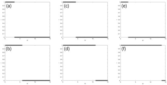
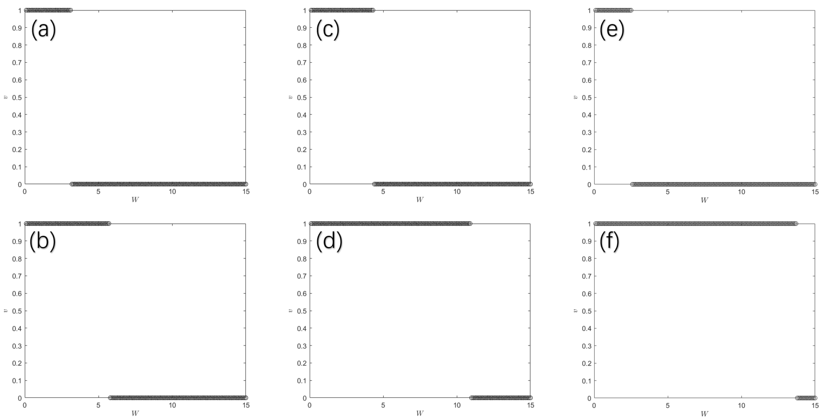
First, we can calculate the real-space winding number of disorder realizations in Figure 4a–d from Equation (2), since we can obtain all eigen-functions from the eigen-equation. The results are shown in Figure 4a–d. For all of the realizations demonstrated, is 1 initially, then it jumps to 0 at a certain value of disorder strength W. This evolution pattern proves that there is TPT for every realization. This also agrees with the disappearance of zero-energy states in Figure 2 in the energy spectra. To demonstrate that the conclusions are universal rather than being restricted to a specific value , we also provide examples for and in Figure 4e,f.
Figure 4.
The evolving of real-space winding number versus disorder strength W for six different realizations, respectively. The system undergoes a TPT when jumps from 1 to 0. (a–d) . (e) . (f) .
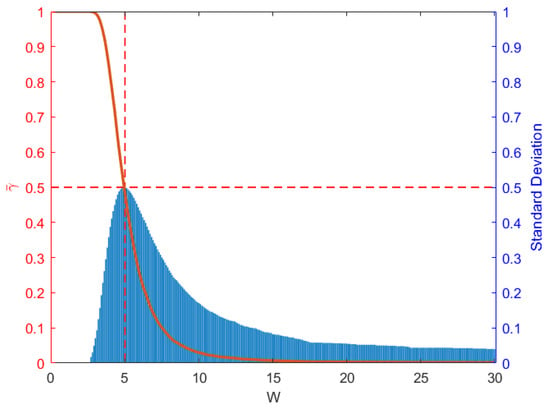
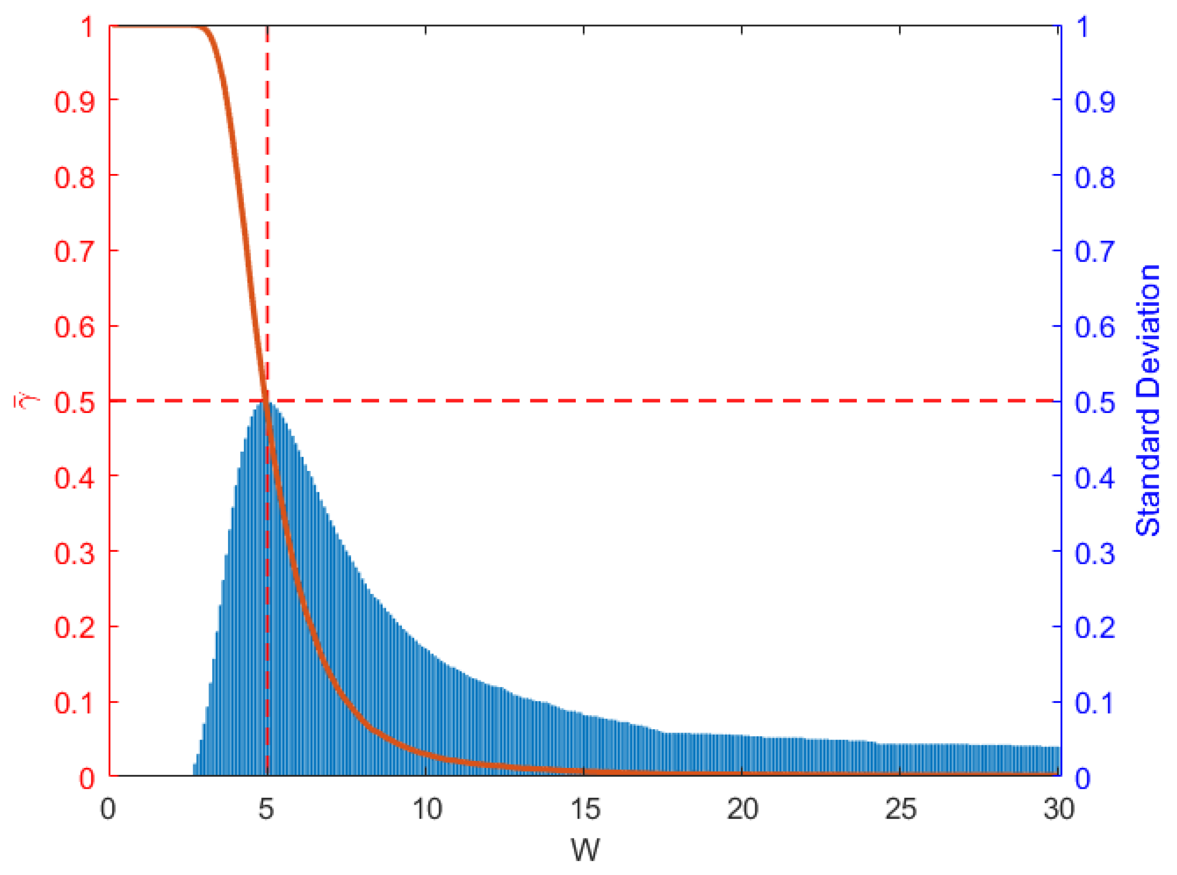
Figure 2, Figure 3 and Figure 4 only present specific realizations. However, as for the disordered model, only the ensemble average can truly reflect the characteristics of the system. So we calculate the ensemble average of real-space winding number [15] with realizations versus the disorder strength W. Based on the eigen-functions of realizations of our model, we can calculate the real-space winding number of all realizations. By the statistical distribution of , we can obtain the average value and the standard deviation of for these realizations versus W, which are shown in Figure 5.
Figure 5.
The ensemble average of the real-space winding number over 10,000 disorder realizations, shown by the red line, and its standard deviation, shown by blue bars, versus disorder strength W. The red dashed line denotes the TPT point, defined by . It is clearly shown that there is a TPT, since the ensemble average decreases from 1 to near-zero value when the disorder strength W increases.
From Figure 5, we observe the following characteristics. First, the initial equals to 1 when , which agrees with our expectation. Second, with the increase in disorder strength, keeps almost unchanged when and the standard deviation is zero, also. Third, when , starts to decrease and the standard deviation increases quickly. Forth, decreases from 1 to almost zero in the range . This clearly shows that there is a TPT in this process statistically. In this work, we define the critical point of the TPT as . For this model, we find critical point at , which is signified by the dashed line in Figure 3. Fifth, at the critical point, the standard deviation gets to its maximum value , which is same as the average value.
Comparing the evolution process in Figure 5 with the spectrum of one realization shown in Figure 2, we can see some interesting points. First, when , we observe unit and zero fluctuation in Figure 5. Also, in this disorder strength range, we observe that the gap does not close for almost all random realizations in Figure 5. Actually, the W is not a small value anymore in this range, and the localization length is only several cell lengths. This means that the system is topologically nontrivial even when the wavefunctions are quite localized. So, the topological property is quite robust against disorder for SSH model. Second, when the disorder strength is strong enough to cause the close of the gap and the disappearing of topological edge states for some realizations, the starts to decrease and the standard deviation starts to increase in Figure 5. So the decrease in is from the starting of TPT for certain realizations. Third, at critical point , there is exactly half of the realizations have passed the phase transition, so that the standard deviation arrives at its maximum , also. Forth, when W is very large, e.g., , the standard deviation is still not zero, which means that some rare realizations have not passed the phase transition yet. This is quite significant, since the W is about six times larger than at this point. We looked into one of the rare realizations, which is topologically nontrivial when W is 29, and found some characteristics with its random number (this will be discussed later in Section 5).
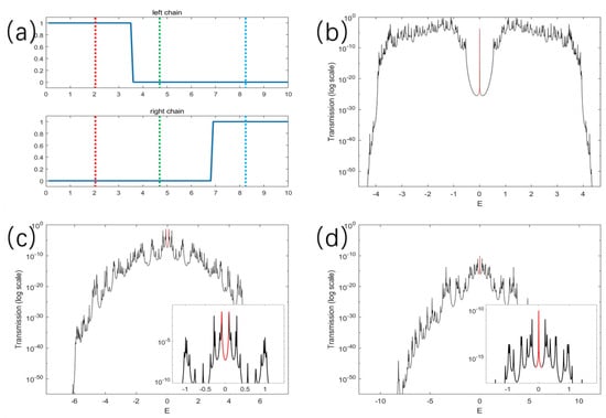
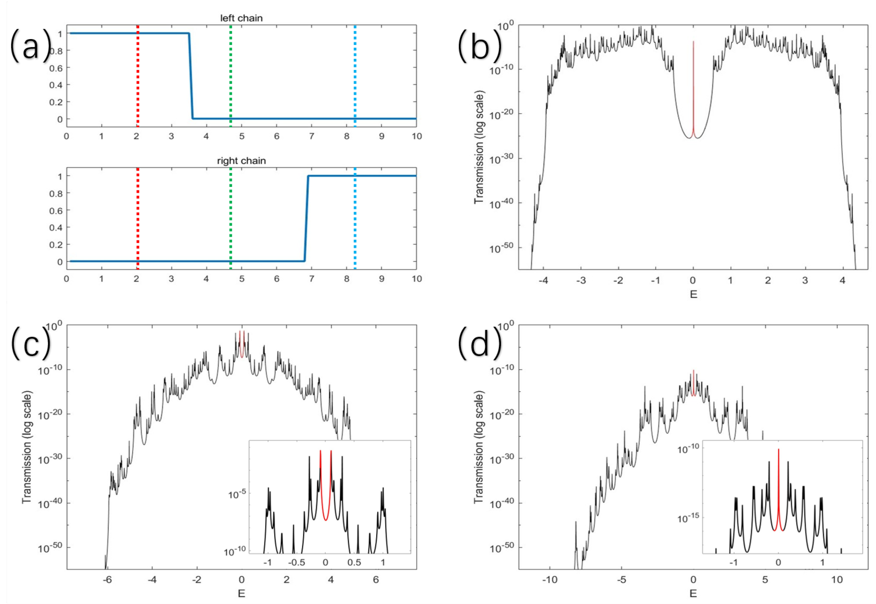
However, end states are not genuinely topological, since both phases are adiabatically connected to the atomic limit [21]. In contrast, the interface (domain-wall) states between regions with distinct topological invariants provide a more direct manifestation of topological protection, as they are guaranteed by bulk–boundary correspondence. We construct an interface between two SSH chains belonging to two different regions or the same region of disorder-induced topological phases. Then, we observe the evolution of the corresponding interface state with increase in disorder strength W, with gap at first or with gap closed while W is large enough. By considering two distinct scenarios—where the critical points of the left and right SSH chains are either the same or different—we systematically track the occurrence and disappearance of the interface state. We find that the occurrence or disappearance of the zero-energy edge state really corresponds to the theoretical prediction based on the topological phases of two SSH chains. For the first case, originally two periodic SSH chains are conjugated with each other and their disorder realizations are also same. So, they share the same TPT point. Before and after the critical point, both of them go through the topological phase transition. So, the left and right SSH chains always have different topological phases. According to our theory, the interface state should always exists with gap or with the gap closed. The observed phenomena of interface state, agrees with our theory very well.
As the first case is a subset of the second case, we will display the second case in detail. For the second case, originally, two periodic chains are also chosen to be conjugated with each other with different topological phases. But the disorder realizations of two chains are chosen to be different. So they have different TPT points, as shown in Figure 6a. With the increase in W, the two SSH chains initially reside in topologically distinct phases, then transition into the same phase, and eventually become topologically distinct again. According to our theory, in the process, correspondingly, the interface state first exists, then disappears, and finally occurs again. The numerical results, shown in Figure 6b–d, agree with our theoretical prediction very well. These results provide strong evidence for the presence of nontrivial interface physics between disorder-induced topological phases, thus improving the physical interpretation of the disorder-induced TPT.
Figure 6.
Evolution of the interface state in a composite SSH chain. (a) Real winding number (RWN) of the two individual SSH chains as a function of disorder strength before coupling. (b) Composite phases corresponding to the red vertical line in (a), where an interface state appears within the gap. (c) Composite phases corresponding to the green vertical line in (a), where the interface state disappear from the gap. (d) Composite phases corresponding to the blue vertical line in (a), where an interface state reemerges in the gap.
3.3. Different Pictures for TPT
From the real-space winding number, we demonstrate that there is a TPT for our model. But the physical picture for such TPT process for disorder systems has not been well studied so far, and the critical point of such disorder systems cannot be predicted generally.
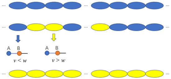
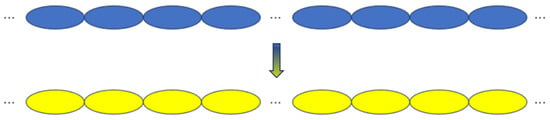
The first picture of TPT process is “the gradual change picture”. We suppose that the disordered system is composed by the local cells. For the pure periodic system of the SSH model, the topological property is determined by the relative size of intracell hopping and intercell hopping. Based on this idea, we can intuitively propose a “gradual chain inversion process”, which can be described by the “partial inversion” of disordered SSH chain. The so-called inversion refers to the change of the relative size between the local intracell and local intercell hopping terms and . The gradual picture of the process is shown in Figure 7.
Figure 7.
Schematic diagram of the gradual change picture of the TPT with the local chain inversion process. The blue ellipse represents unit cells whose intracell hopping is smaller than the intercell hopping, and the yellow ellipse represents unit cells whose intracell hopping is larger than the intercell hopping. With the local inversion of hopping terms, the model gradually goes through the TPT.
In Figure 7, the ellipses of different colors represent unit cells with different relative sizes between intracell and intercell hopping terms. In detail, the entire SSH chain under a clean limit is composed of blue ellipses in the initial state. With the gradual increase of disorder strength W, the added values of and of intracell and intercell hopping terms and will also increase differently due to the existence of ratio k. Considering that every lattice is with random disorder strength, the magnitude of this increase is not certain, and it may be the case that is still smaller than . But in general, because of the existence of ratio k, the intercell hopping term should increase less than the intracell hopping term . So the relative size between the intracell and intercell hopping terms of some unit cells inverses from the initial state, smaller than , to the new state, larger than . This corresponds to the Figure 7, where some blue ellipses are gradually transformed into yellow ellipses. Finally, when the disorder strength is large enough, the difference between and is greater than the difference between and in the initial state. At this time, all blue ellipses are transformed into yellow ellipses and all unit cells are inversed. So the TPT occurred.
However, this gradual inversion picture is also quite unnatural in some way. First, such a gradual inversion picture is not compatible with the sudden change picture of topology. Since topology is the basic connectivity property of the geometry, the topological phase transition generally is the “sudden change picture”, e.g., a hole is generated on the space. Second, we also find that if we change a hopping term from to , which does not change any relative size of the hopping terms locally, the total topology, signified by the real-space winding number of a realization of the disordered SSH model, will change.
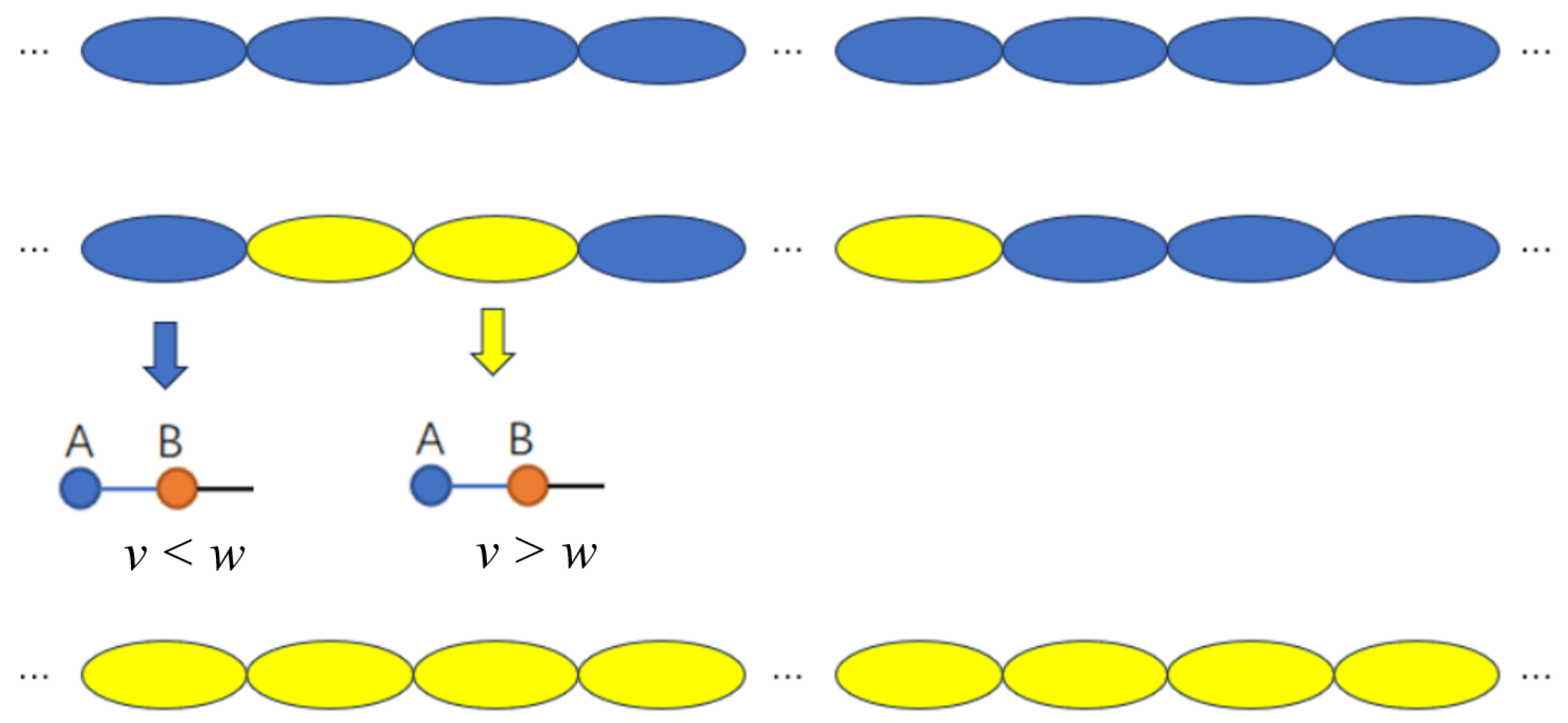
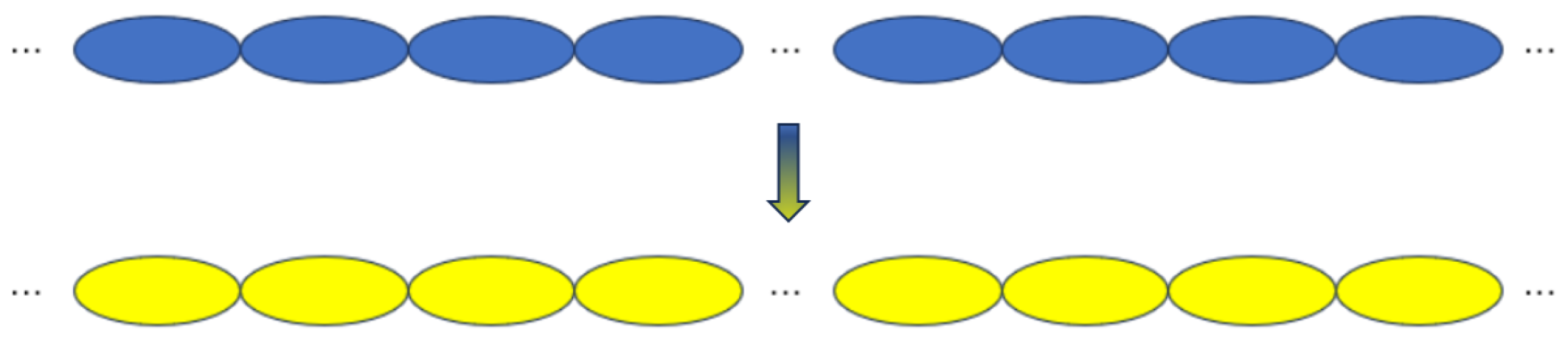
Therefore, we can assume second picture of TPT process which is the sudden change picture. In Figure 8, we show the sudden change picture of the TPT schematically, whose topology is a global property and can be suddenly changed globally in the TPT process. Briefly, the idea is to represent the entire disordered SSH chain in terms of two effective sublattices so that crossing the critical point impacts the behavior of the entire chain. This picture is quite anti-intuition, and we will show that it is a correct picture of the TPT of the disordered SSH model.
Figure 8.
The schematic diagram of the sudden change picture of the TPT for the disordered SSH model. From the blue topological nontrivial chain, the model is suddenly changed into a yellow topological trivial chain, or vice versa.
3.4. Different Means of Hopping Terms Versus TPT Point
In our assumption about the chain inversion process, we naively guessed that the TPT point of such a disordered system is still determined by the relative size of arithmetic mean of disordered intracell hopping and intercell hopping. Next, we will show that this naive guess is not correct. The critical point is determined by another mean value of disordered hopping terms, and the physical reason behind it is very inspiring for us to understand the TPT of disorder systems.
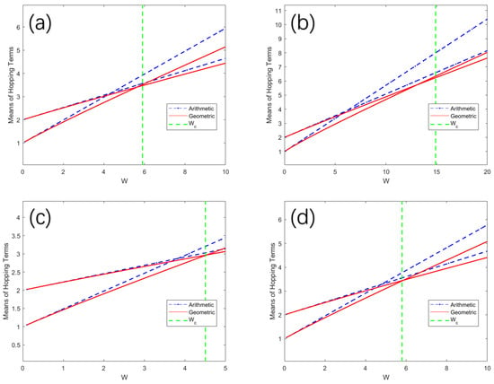
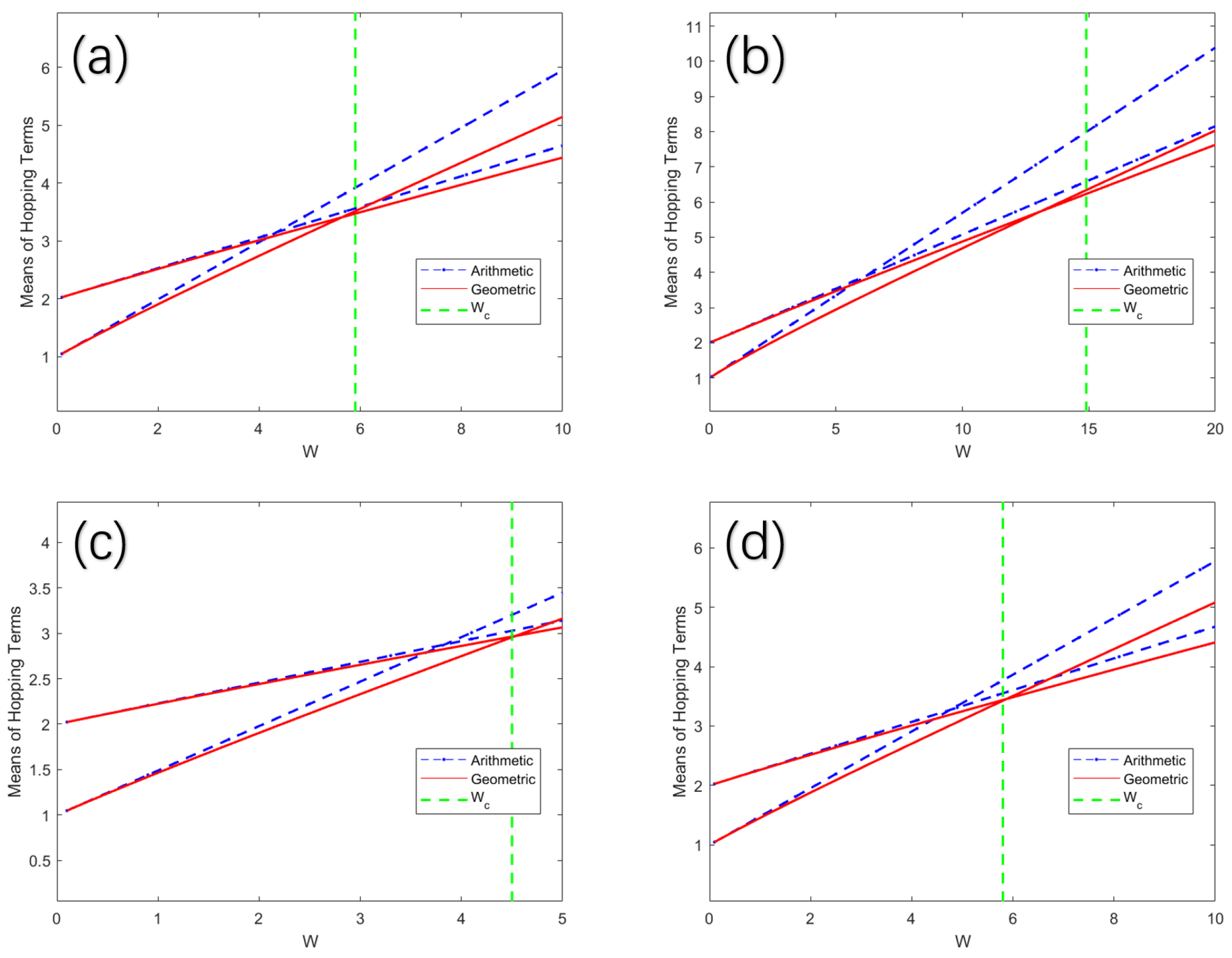
First, we start from different realizations and try to find the relation between the TPT with the arithmetic mean values. But we immediately find that the relative size reversal of the arithmetic mean values of intracell and intercell hopping terms does not correspond to the phase transition point. Then, we try the geometry mean values of the intracell and intercell hopping terms. These results versus disorder strength W are shown in Figure 9. In Figure 9, each blue dashed line represents the arithmetic mean value of intracell and intercell hopping terms, while each blue solid line represents the geometry mean value of intracell and intercell hopping terms. Obviously, each intersections of the solid lines and the dashed lines are the cases where the mean values of intracell hopping terms and intercell hopping terms are equal. The vertical green line signifies the of the critical point of TPT for every realization. From Figure 9, we can see that the intersections of red solid and dashed lines, representing geometric mean values, provide a better correspondence to the critical disorder strength , whereas the intersections of blue lines , representing arithmetic mean values, are generally much smaller than .
Figure 9.
The arithmetic and geometric mean values of the hopping terms of four different realizations vs disorder strength W. (a) The 1Oth realization; (b) The 48th realization; (c) The 56th realization; (d) The 245th realization. The blue lines and red lines show the arithmetic and geometric means of the intracell and intercell hopping terms; the green line indicates the critical disorder strength of each realization defined by the jumping point of real space winding number. It is evident that the intersection of the red lines coincides with the green line in each realization, whereas that of the blue lines does not. There is about a deviation in (b), which will be discussed later.
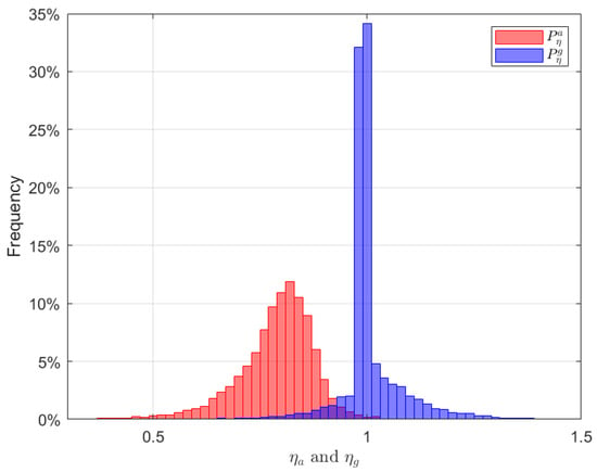
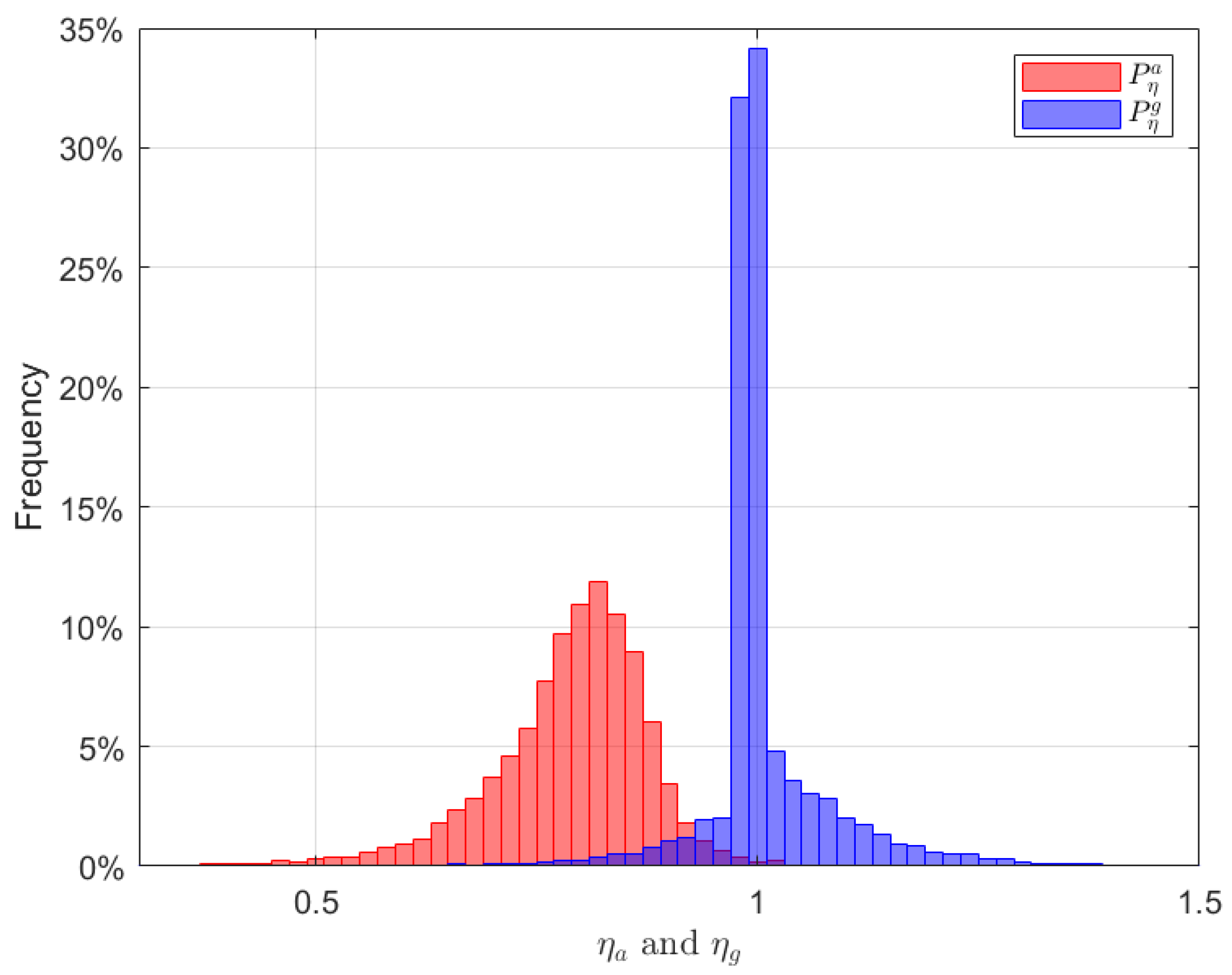
To further validate our observation, we obtain the ratios of the intersection point of those mean values to of 10,000 realizations and draw the probability distribution of these realizations in Figure 10, where denotes the ratios of the of intersection of arithmetic mean values to , and denotes the ratios of the of the intersection point of geometric mean values to . First, we can see that the distribution of for arithmetic mean is located well below 1, while the distribution of for geometry mean is around 1. Second, the distribution of is expanding in a wide range, while the distribution of is very focusing. Figure 9 clearly demonstrates an excellent microscopic correspondence of and , while Figure 10 further shows that this correspondence is well preserved statistically. Therefore it strongly supports our conclusion that the intersection point of geometric mean values can be used to predict the critical value of TPT points .
Figure 10.
The distribution of and of 10,000 realizations by r, where and are the ratio between the disorder strength of the intersections of the arithmetic means and geometric means to the disorder strength of the critical point of a certain realization. We can see that is focused at , while is widely distributed in a range from 0.65–0.85.
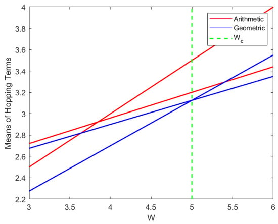
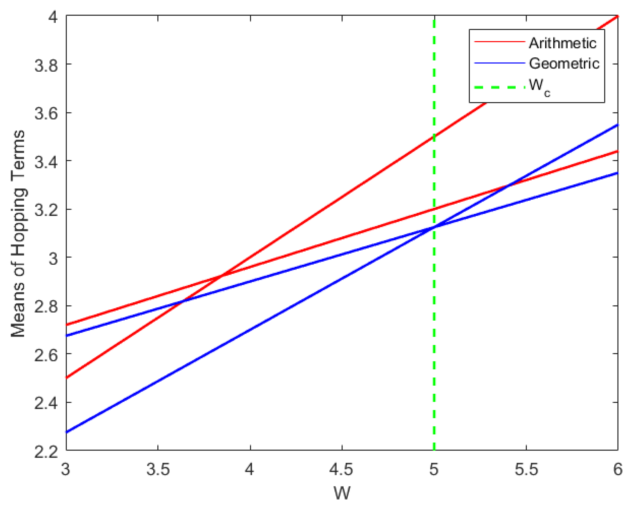
Figure 10 shows the correspondence for every realization. We also need to demonstrate the correspondence for ensemble average for the disordered SSH model. The results of the arithmetic and geometric mean values of intracell and intercell hopping terms over 10,000 disorder realizations are shown in Figure 11. We observe the following characteristics. First, initially the mean value of the intercell hopping terms is bigger than that of the intracell hopping terms. It agrees with the initial parameters of our model. Second, the mean value of the intercell hopping terms is increasing more slowly than that of the intracell hopping terms. This is because the ratio k is smaller than 1. Third, the arithmetic means (blue lines) are larger than the geometric means (red lines). Forth, when the intersection of the red lines happens, the disorder strength of the intersection matches to the critical value of the TPT point, the same as shown in Figure 5. However, the arithmetic means of hopping terms intersect at the disorder strength , which does not agree with the critical value . We further investigate this property by calculating the geometric means of hopping terms under different initial parameters, and find a same uniformity of the intersection point and the critical value . Obviously, the critical point is determined by the geometric mean values of intracell and intercell hopping terms. We may draw a preliminary conclusion that the TPT will occur when the geometric means of intracell hopping terms equals to the geometric means of intercell hopping terms.
Figure 11.
The arithmetic and geometric mean values of hopping terms over 10,000 disorder realizations versus the disorder strength W. The red line denotes the arithmetic means of the intracell hopping terms and the intercell hopping terms. The blue line represents the geometric means. The green line denotes the mean critical value of the disorder strength of the TPT point . Obviously, the intersection of the blue lines corresponds to the TPT point for the ensemble average.
4. Discussion and Theory
In this section, we will construct the theory to predict the critical point of TPT of a disordered SSH model. We can theoretically demonstrate that the critical point corresponds to the intersection of the geometric means of the hopping terms, which agrees with the observations of our numerical results in Section 3.3.
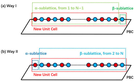
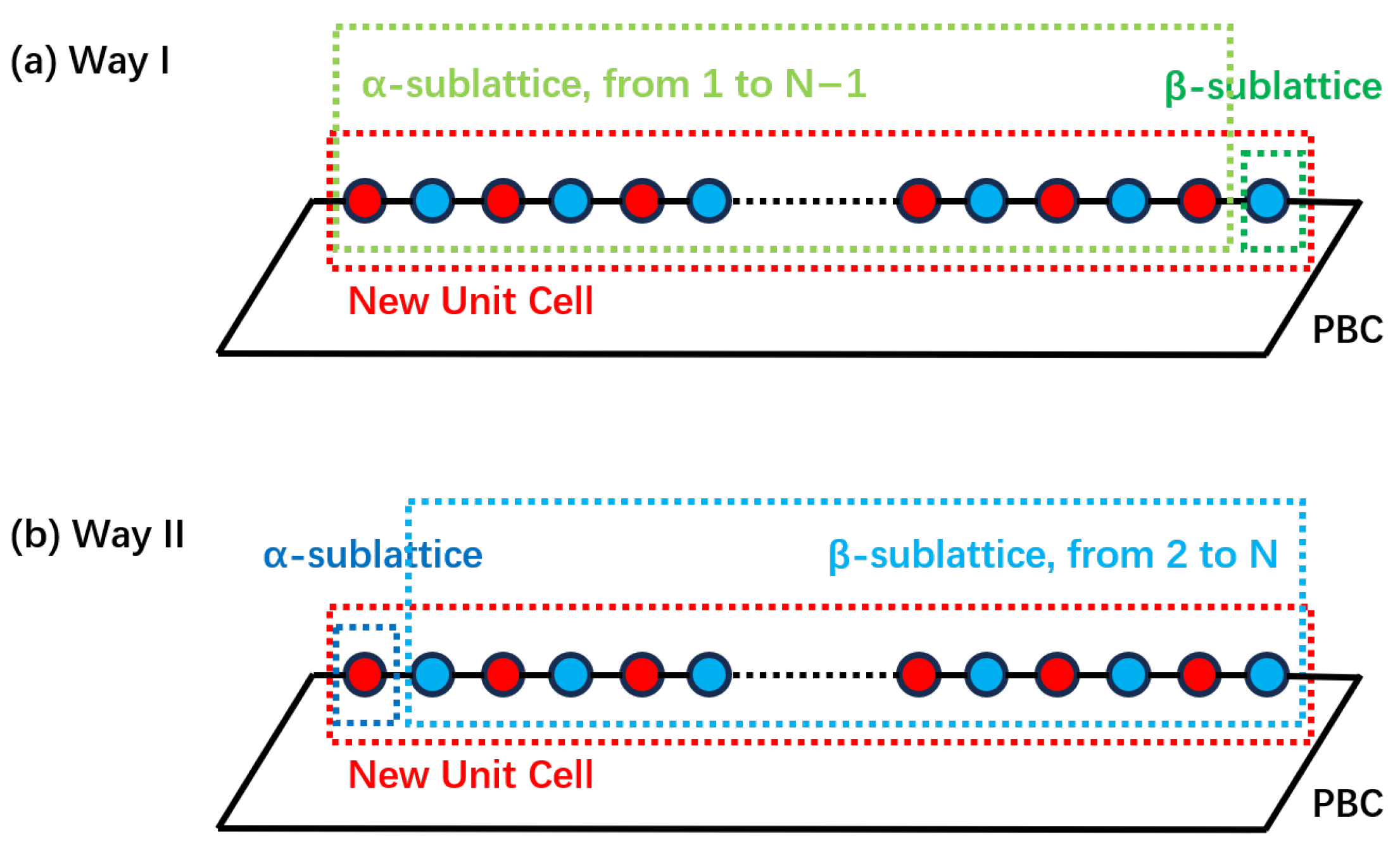
First, we consider a N-lattices disordered SSH model with periodic boundary condition (PBC), which is widely used in topological studies of disordered systems [2,3,5,15] and also used in our calculation of real-space winding number. Since the periodic boundary condition, the total N-lattices disordered SSH model can be thought as a new unit cell of infinite periodic system, as shown in Figure 12. Following another work from our group [22], we can redefine the sublattices of the new cell in two methods. The first method I is to define that the cell contains the -sublattice, which consists of the 1st to st lattices of the N-lattice disordered SSH model, and the -sublattice, which consists of only the Nth lattice of the N-lattice disordered SSH model, as shown by the green squares in Figure 12a. The second method is to note that the cell contains the -sublattice, which consists of only the 1st lattice of the N-lattice disordered SSH model, and the -sublattice, which consists of the 2nd–Nth lattices of the N-lattice disordered SSH model, as shown by the blue squares in Figure 12b.
Figure 12.
Two methods to redefine the sublattices of the finite disordered SSH model with N lattices, which is thought of as a new cell since the periodic condition is applied. In (a), we redefine the lattices from 1 to of the disordered SSH model as the -sublattice and the N lattice as the -sublattice. In (b), we redefine the 1 lattice as the -sublattice and the lattices from 2 to N as the -sublattice.
Then the Hamiltonian of -sublattice of I-method can be expressed as
Similarly, the Hamiltonians of the -sublattice of -method can be expressed as
where the means the hopping from the lattice to , etc.
Since and are SSH chains with odd lattices (), each of them must have a chiral zero-energy edge state [23]. We can obtain the chiral edge state by resolving the determinant and . The results are given by
where and are normalization coefficients. For convenience in the following derivation, we denote
For the classical SSH model, the condition for a TPT is that the intracell hopping term equals the intercell hopping term. By redefining the sublattices in method I or , we can map a realization of the N-lattice disordered model under PBC to an effective classical SSH model where each cell contains two sublattices.
As shown in Figure 12, the effective intracell hopping term is the hopping from -sublattice to -sublattice, and the effective intercell hopping term is the hopping from -sublattice to -sublattice.
Consequently, similarly to the classical SSH model, the condition for the TPT, where the chiral edge states emerge or disappear, becomes that the effective intracell hopping term equals the effective intercell hopping term:
Following the approach proposed in our recent work [22], the effective intracell and intercell hopping terms for the redefined sublattice in method I and is given by
The left side of Equation (11) is the product of all hopping terms from odd lattice to the even lattice, which corresponds to the intracell hopping terms of the N-lattice disordered SSH model. The right side is the product of all hopping terms from the even lattice to the odd lattice, which corresponds to the intercell hopping terms. Then we can acquire that the condition we derived through super-lattice theory agrees with our discovery in Section 3.4. The result of Equation (11) proves that the TPT will occur when the geometric means of intracell hopping terms equals to the geometric means of intercell hopping terms. This conclusion can be obtained for each realization of our disordered SSH model, thus being valid for the ensemble average.
Such a redefinition of the sublattices and the theoretical conclusion that the geometric means, not the arithmetic means, determines the TPT may appear counterintuitive. Obviously, the geometric means is very sensitive to the value of the single hopping term, while the arithmetic means seems more robust. However, it reflects the physical origin of the TPTs of this disordered system. By redefining the N-lattice 1D disordered SSH model to two effective sublattices, we effectively restore the underlying sub-symmetry of the system [22]. The TPT of the system is then again determined by the effective intercell and intracell hopping terms of the newly redefined sublattices, just like the conventional SSH model. This perspective also clarifies the physical picture of the TPTs of our model in Section 3.3 of this work. The TPT is not from a gradual local-changing picture, which we used to naively believe that local transitions accumulate and lead to a TPT, but rather a global sudden change picture.
5. Other Models with Different and k
In this section, we will apply our theory to other 1D disordered SSH models and prove its validity. We will first introduce the new models, then investigate the real-space winding number and calculate the products of the hopping terms. We can numerically demonstrate that the critical point is corresponding to the intersection of products of odd and even hopping terms, which agrees with the theoretical results of Equation (11).
5.1. Results for the Model with
We first introduce a variant of our 1D disordered SSH model. As introduced in Section 2, the Hamiltonian is given by
where the parameters remain the same except for the random numbers and , which are defined with the rectangular distribution in the range now.
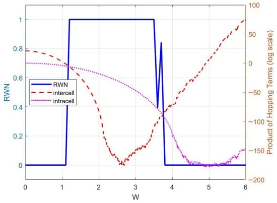
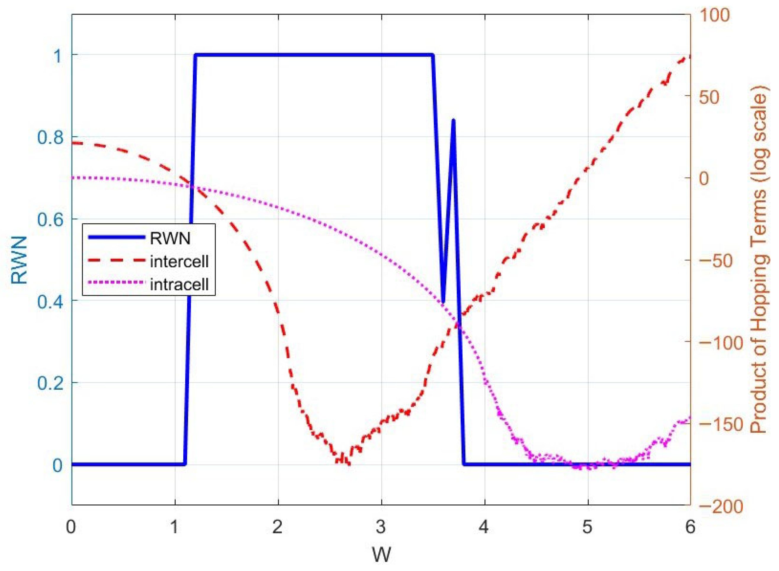
The change in the range of and causes some differences. Since the hopping terms could be negative, the geometric means of the hopping terms are not available anymore. However, based on Equation (11), we can directly calculate the products of the intercell and intracell hopping terms and compare the size of them. The results of four realizations are shown by Figure 13.
Figure 13.
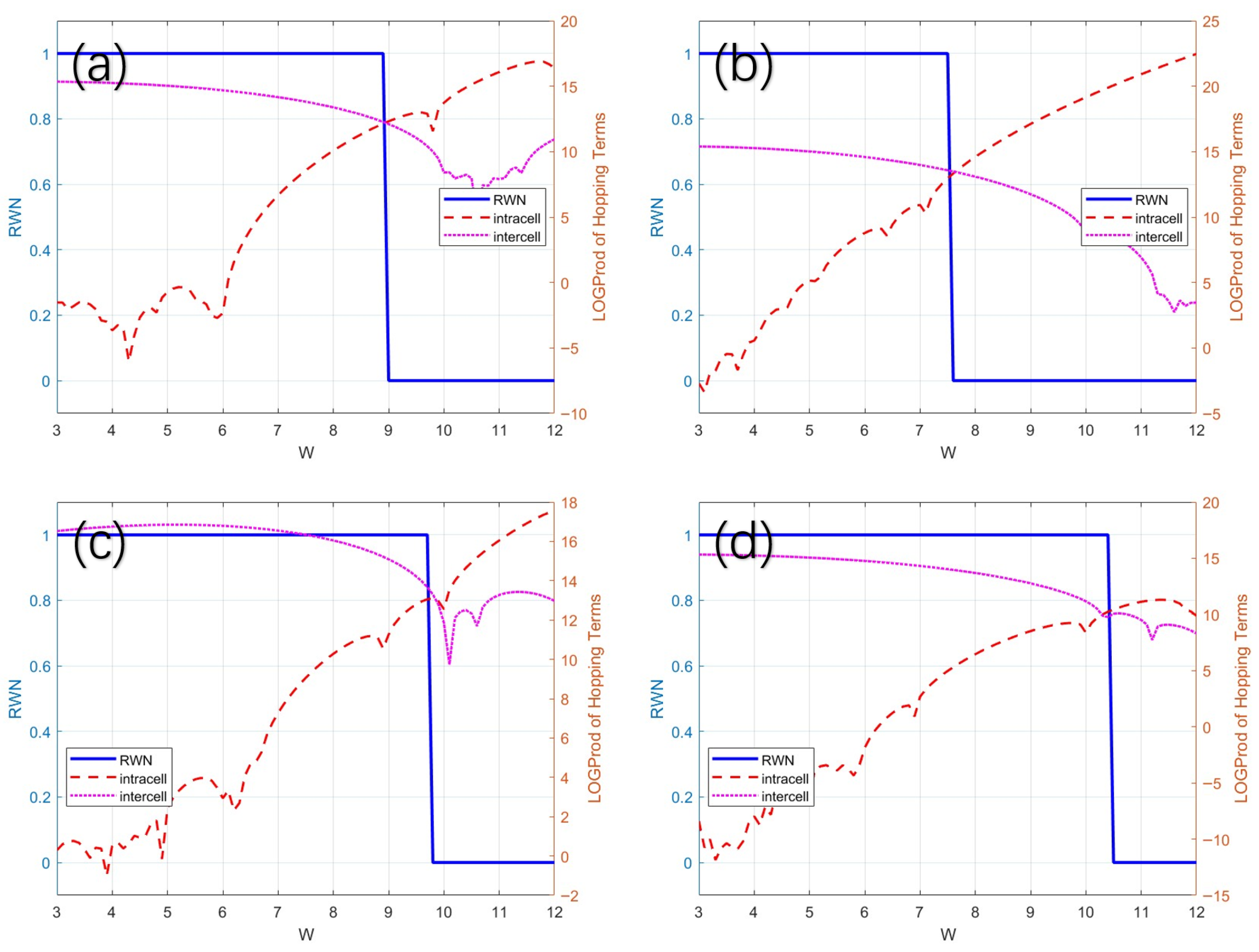
The absolute value of the product of the intercell and intracell hopping terms versus the disorder strength W of different realizations, which are shown by pink and red dotted lines on a logarithmic scale. (a) The 233th realization; (b) The 487th realization; (c) The 520th realization; (d) The 888th realization. The blue line shows the development of the real-space winding number of the realizations versus W. Obviously, the intersections of the pink and red lines approximately coincide with the TPT point.
In Figure 13a, the blue line shows the real-space winding number of the model, and the pink and red dot lines respectively show the products of the intercell and intracell hopping terms, which are plotted on a logarithmic scale. The realization has a TPT point at , while the product of the intercell and intracell hopping terms also have an intersection at . Figure 13b also show the same conclusion. Our theoretical result in Equation (11) is verified numerically for this model.
For realizations like Figure 13c,d, the intersection does not exactly coincide with the critical TPT point. Such a deviation is because of the large fluctuations around the TPT point, which are generally caused by some hopping terms whose values are very small. In such cases, the TPT point could be more accurately characterized by the intersection of envelopes of the pink and red lines rather than by the lines themselves.
5.2. Results for the Model with
Another model, the same as that in [17], was also investigated, where the initial hopping terms are and the random numbers are defined with the rectangular distribution in the range and the lattice number is . In Figure 14, we select a single realization and show the real-space winding number as a function of W by the blue line, with a plateau indicating two TPTs at different values of W. We then compute the products of the intercell and intracell hopping terms, which are represented by the pink and red lines, respectively. We observe that, for the two critical TPT points, which are revealed in [17], there remains a clear correspondence with the intersections of pink and red lines. The conclusion of Equation (11) remains valid, as shown in Figure 14. Even more so, the strong phase fluctuation around second TPT (from ungapped TAI to trivial phase) can also explained from the large fluctuation of the products of the intercell and intracell hopping terms.
Figure 14.
The product of the intercell and intracell hopping terms versus disorder strength W for a typical realization for the model with . The blue line shows the development of the real-space winding number of the realizations versus W. We can see that two intersections still correspond to the two TPT points of the model.
5.3. Results for the Model with Different k
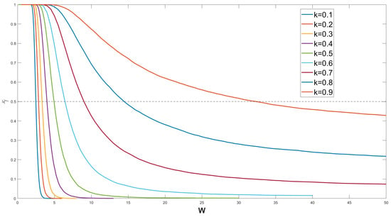
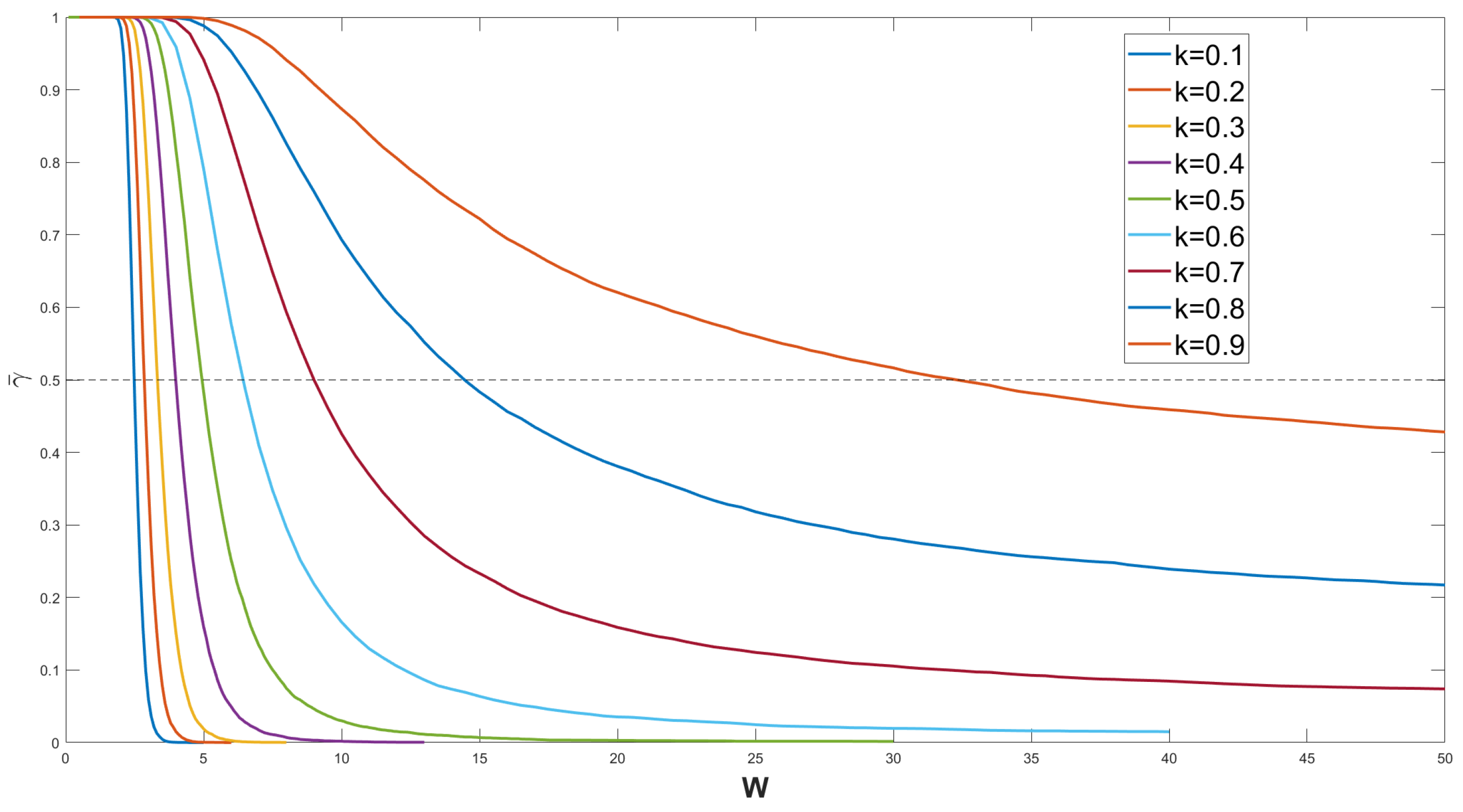
Models with different k were also investigated. First, the ensemble average of the real-space winding number as a function of W over 10,000 disorder realizations for different values of k is shown in Figure 15. Due to our choice of initial parameters, and , k was restricted to be less than 1 to ensure the TPT. The nine curves in the figure, from left to right, correspond to . All of the curves stably cross the dashed line , indicating the occurrence of a TPT. As discussed in Section 3.3, the smaller the value of k, the smaller the critical W at which the TPT occurs.
Figure 15.
The ensemble average of the real-space winding number over 10,000 disorder realizations, shown by colored lines, versus disorder strength W are presented. The dashed line denotes the TPT point defined by . It is clearly shown that there are TPTs, since the ensemble average decreases from 1 to near-zero value when disorder strength W increases.
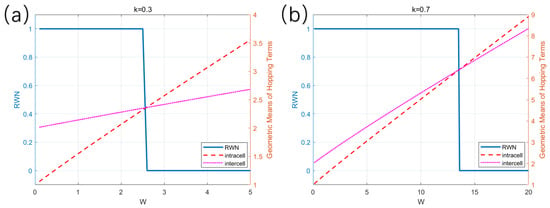
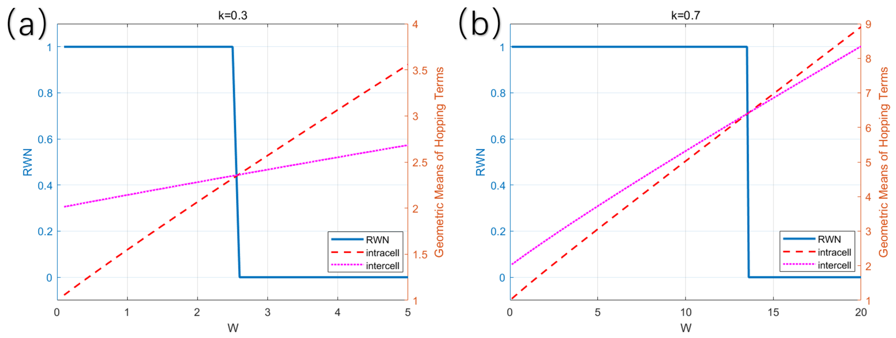
Also, the intersection point of geometric mean values still can be used to predict the critical value of TPT points . We present two examples, corresponding to one realization with and one realization with , as shown in Figure 16a,b. The geometric mean values of intracell and intercell hopping terms are shown by red and pink dashed lines. The blue line represents the real-space winding number (RWN) versus W. Obviously, the intersection of pink and red dashed lines corresponds to the TPT point of the realization.
Figure 16.
Intersection of geometric mean values of intracell and intercell hopping terms corresponding to the TPT point of the realization. The red line denotes the geometric mean values of intracell hopping terms. The pink dashed line denotes the geometric mean values of intercell hopping terms. The blue line represents the real-space winding number (RWN) versus W. (a) . (b) .
The results of those models with different parameters show that our theory does not rely on model details. This theory does not depend on the type of disorder: it holds for different disorder distributions described by , different realizations, and different values of the ratio k. Once the product of the intercell and intracell hopping terms equal to each other, TPT will occur in the realization. With the models discussed above, we demonstrate the validity of our theory.
6. Conclusions
In conclusion, we have studied the topology of a general 1D disordered SSH model with two tunable parameters, a disorder distribution center , and a ratio k between the disorder strengths of the intracell and intercell hopping terms. Several important conclusions are obtained. First, by means of numerical calculations and the real-space winding number, we find that the model generally exhibits TPTs. Second, the critical TPT points are determined by the intersections of the products (or geometric means) of the intercell and intracell hopping terms. Third, we develop the theory for such a general 1D disordered model by redefined the sublattices of our model. We demonstrate that the TPTs are governed by the products of the odd and even hopping terms, and when they are equal to each other, the TPT will occur. Fourth, based on both the analysis of numerical results and theoretical derivation, we establish the physical picture of TPT of 1D disordered models, which is a sudden global transition for the whole system. We also reveal the sub-symmetry origin of the TPT of the disordered SSH model.
Further work on this topic may be extended by incorporating next-nearest-neighbor (NNN) hopping or on-site potential disorder, exploring non-Hermitian perturbations, applying to other STI systems, or generalizing the framework to higher-dimensional systems, such as the ladder-like Kitaev chain. Such developments could induce richer disorder-induced phase diagrams and new classes of topological phenomena. Broadening the disordered topological models to various physical platforms could lead to novel applications, including acoustic, photonic, and mechanical systems.
Author Contributions
Conceptualization, X.W.; methodology, X.W.; software, X.W.; formal analysis, X.W. and Y.L. (Yunlin Li); data curation, X.W., Y.L. (Yufu Liu), Z.L. and Y.H.; writing, X.W.; supervision, X.J. All authors have read and agreed to the published version of the manuscript.
Funding
This research received no external funding.
Institutional Review Board Statement
Not applicable.
Informed Consent Statement
Not applicable.
Data Availability Statement
The original contributions presented in this study are included in the article. Further inquiries can be directed to the corresponding author.
Conflicts of Interest
The authors declare no conflicts of interest.
References
- Heeger, A.J.; Kivelson, S.; Schrieffer, J.R.; Su, W.-P. Solitons in conducting polymers. Rev. Mod. Phys. 1988, 60, 781–850. [Google Scholar] [CrossRef] [Scilit]
- Zhang, S.; Zhou, Q. A two-leg Su–Schrieffer–Heeger chain with glide reflection symmetry. Phys. Rev. A 2017, 95, 061601. [Google Scholar] [CrossRef] [Scilit]
- Martinez Alvarez, V.M.; Coutinho-Filho, M.D. Edge states in trimer lattices. Phys. Rev. A 2019, 99, 1. [Google Scholar] [CrossRef] [Scilit]
- Zhang, Y. Fractal topological band-gap structure induced by singularities in the one-imensional Thue–Morse system. Photon. Res. 2021, 9, 622–629. [Google Scholar] [CrossRef] [Scilit]
- Li, L.; Xu, Z.; Chen, S. Topological phases of generalized Su–Schrieffer–Heeger models. Phys. Rev. B 2013, 89, 163–167. [Google Scholar] [CrossRef] [Scilit]
- Perez-Gonzalez, B.; Bello, M.; Gomez-Leon, A.; Platero, G. Interplay between long-range hopping and disorder in topological systems. Phys. Rev. B 2019, 99, 035146. [Google Scholar] [CrossRef] [Scilit]
- Bellani, V.; Diez, E.; Hey, R.; Toni, L.; Tarricone, L.; Parravicini, G.B.; Domínguez-Adame, F.; Gómez-Alcalá, R. Experimental Evidence of Delocalized States in Random Dimer Superlattices. Phys. Rev. Lett. 1999, 82, 2159. [Google Scholar] [CrossRef] [Scilit]
- Naether, U.; Stützer, S.; Vicencio, R.A.; Molina, M.I.; Tünnermann, A.; Nolte, S.; Kottos, T.; Christodoulides, D.N.; Szameit, A. Experimental observation of superdiffusive transport in random dimer lattices. New J. Phys. 2013, 15, 013045. [Google Scholar] [CrossRef] [Scilit]
- Hsu, H.C.; Chen, T.W. Topological Anderson insulating phases in the long-range Su–Schrieffer–Heeger model. Phys. Rev. B 2020, 102, 205425. [Google Scholar] [CrossRef] [Scilit]
- Mondragon-Shem, I.; Hughes, T.L.; Song, J.; Prodan, E. Topological Criticality in the Chiral-Symmetric AIII Class at Strong Disorder. Phys. Rev. Lett. 2014, 113, 046802. [Google Scholar] [CrossRef] [Scilit]
- Shapiro, D.S.; Remizov, S.V.; Lebedev, A.V.; Babukhin, D.V.; Akzyanov, R.S.; Zhukov, A.A.; Bork, L.V. Critical phase boundary and finite-size fluctuations in the Su-Schrieffer-Heeger model with random intercell couplings. Phys. Rev. A 2022, 105, 023321. [Google Scholar] [CrossRef] [Scilit]
- Nava, A.; Campagnano, G.; Sodano, P.; Giuliano, D. Lindblad master equation approach to the topological phase transition in the disordered Su–Schrieffer–Heeger model. Phys. Rev. B 2023, 107, 035113. [Google Scholar] [CrossRef] [Scilit]
- Loring, T.A.; Hastings, M.B. Disordered topological insulators via C*-algebras. Europhys. Lett. 2010, 92, 67004. [Google Scholar] [CrossRef] [Scilit]
- Bianco, R.; Resta, R. Mapping topological order in coordinate space. Phys. Rev. B 2011, 84, 241106. [Google Scholar] [CrossRef] [Scilit]
- Lin, L.; Ke, Y.; Lee, C. Real-space representation of the winding number for a one-dimensional chiral-symmetric topological insulator. Phys. Rev. B 2021, 103, 224208. [Google Scholar] [CrossRef] [Scilit]
- Shi, X. Disorder-induced topological phase transition in a one-dimensional mechanical system. Phys. Rev. Res. 2021, 10, 142–149. [Google Scholar] [CrossRef] [Scilit]
- Mina, R. Realization of Gapped and Ungapped Photonic Topological Anderson Insulators. Phys. Rev. Lett. 2024, 132, 066602. [Google Scholar] [CrossRef] [Scilit]
- Fulga, I.C.; van Heck, B.; Edge, J.M.; Akhmerov, A.R. Statistical topological insulators. Phys. Rev. B 2014, 89, 155424. [Google Scholar] [CrossRef] [Scilit]
- Markoš, P.; Soukoulis, C.M. Wave Propagation: From Electrons to Photonic Crystals and Left-Handed Materials; Princeton University Press: Princeton, NJ, USA, 2008. [Google Scholar]
- Chen, L. Disorder dependence of helical edge states in HgTe/CdTe quantum wells. New J. Phys. 2014, 14, 043028. [Google Scholar] [CrossRef] [Scilit]
- Traverso, S.; Sassetti, M.; Traverso Ziani, N. Emerging topological bound states in Haldane model zigzag nanoribbons. npj Quantum Mater. 2024, 9, 9. [Google Scholar] [CrossRef] [Scilit]
- Li, Y.; Liu, Y.; Wang, X.; Zhang, H.; Jiang, X. General theory for nonzero subsymmetry-protected topological chiral boundary states. Phys. Rev. Res. 2026, 8, 013256. [Google Scholar] [CrossRef] [Scilit]
- Anastasiadis, A.; Styliaris, G.; Chaunsali, R.; Theocharis, G. Bulk-edge correspondence in the trimer Su–Schrieffer–Heeger model. Phys. Rev. B 2022, 106, 085109. [Google Scholar] [CrossRef] [Scilit]


Disclaimer/Publisher’s Note: The statements, opinions and data contained in all publications are solely those of the individual author(s) and contributor(s) and not of MDPI and/or the editor(s). MDPI and/or the editor(s) disclaim responsibility for any injury to people or property resulting from any ideas, methods, instructions or products referred to in the content. |
© 2026 by the authors. Licensee MDPI, Basel, Switzerland. This article is an open access article distributed under the terms and conditions of the Creative Commons Attribution (CC BY) license.