Proposal of a Modified Loss Function with the Gaussian Copula Density Function to Improve LSTM Predictions of PM₁₀ and PM_2.5 Concentrations

Abstract

Air pollution forecasting for Particulate Matter (${\mathrm{PM}}_{10}$ and ${\mathrm{PM}}_{2.5}$) is a challenge for human health in order to improve the life quality of humans around the world. This research focuses on evaluating a Long Short-Term Memory (LSTM) neural network model with an improvement in the loss function using the Gaussian Copula Density function to predict ${\mathrm{PM}}_{10}$ and ${\mathrm{PM}}_{2.5}$ levels in four stations (AJM, CAM, MER and PED) in Mexico City. The model is compared with a plain LSTM neural network model for forecasting 12, 24, 48 and 72 h using error metrics root mean square error (RMSE), mean absolute error (MAE) and mean absolute percentage error (MAPE). The results demonstrate a superior performance of the modified loss function model, achieving the lowest error values across multiple stations and forecast horizons.

1. Introduction

Today, air pollution is an important concern for human health. Every year, thousands of people experience the effects of living in polluted areas, causing different health problems and, in some cases, even worse [1]. One of the primary air pollutants is particulate matter (PM), specifically ${\mathrm{PM}}_{10}$ and ${\mathrm{PM}}_{2.5}$ particles, which have small diameters of $10\mathsf{\mu }$m or $2.5\mathsf{\mu }$m, respectively [2].

Therefore, it is imperative to assess particulate matter concentrations in urban environments, where the majority of the global population resides. Fortunately, recent advancements in science and technology have facilitated the emergence of innovative methodologies for analyzing contemporaneous particulate matter levels and forecasting future concentrations [3] and predicting future levels [4,5,6].

One of these emerging techniques is Artificial Intelligence (AI), specifically neural networks, which are now widely applied in various fields [7]. An example of such an application is the prediction of the levels of particles in urban areas [4,5,6]. In this research, the technique used is the Long Short-Term Memory (LSTM) Neural Network, a powerful tool with diverse applications, which will be used to predict particulate matter levels for ${\mathrm{PM}}_{10}$ and ${\mathrm{PM}}_{2.5}$.

An important advancement in this neural network is the integration of an advanced statistical technique called Copulas, specifically Gaussian copulas [8]. A copula is a function that is used to model the dependence between random variables [9]. This approach separates the dependence structure from the individual marginal distributions [10,11].

This statistical technique can be used in the loss function of an LSTM neural network model to reduce the model error during training and testing by applying a penalty based on the Gaussian copula density function to improve the prediction of the levels of particles ${\mathrm{PM}}_{10}$ and ${\mathrm{PM}}_{2.5}$ for 12, 24, 48 and 72 h in the metropolitan area of Mexico City.

These results are compared with a basic LSTM neural network using the same hyperparameters and standard error metrics such as root mean square error (RMSE), mean absolute error (MAE) and mean absolute percentage error (MAPE); these error metrics show whether the performance of the new loss function proposed is useful or not in the forecasting of ${\mathrm{PM}}_{10}$ and ${\mathrm{PM}}_{2.5}$ particles.

2. Background

2.1. Urban Airborne Pollution

Air pollution is a complex mixture of particulate matter (PM), gases, and organic and inorganic compounds present in indoor and outdoor air [2]. Currently, air pollution is a global public health problem because it is one of the five leading risk factors for mortality worldwide [1].

Air pollution is determined by the presence of pollutants in the air in large quantities over extended periods [12]. Most of the global population resides in places where the air pollution levels exceed the World Health Organization (WHO) health-based air-quality guidelines [13]. Airborne pollutants include dispersed particles, hydrocarbons, CO, CO₂, NO, NO₂, SO₃, particulate matter, among others including carbonaceous aerosol particles [12,13].

As mentioned before, air pollution poses a considerable risk to human health. Several studies [13,14,15,16] have shown that long exposure to high levels of air pollution can cause numerous health implications such as reduced lung function, incidence of asthma, increased allergic response, lung cancer, or other types of cancer. Another study [17] has shown that air pollution could even affect mental health.

Particulate Matter

Particulate matter (PM) nowadays is one of the most common air pollutants with a complex combination of particles and gaseous substances [18], composed of acidic organic chemicals, metals, and dust particles [19]. The sources where these particles come from can be natural (sea spray, volcanoes, forests, and deserts) or anthropogenic (combustion processes, mechanical or industrial, vehicular emissions and cigarette smoke). This can be named as the primary source [18,19].

Particulate matter is primarily classified into two types, which are particles with a diameter $<2.5$ $\mathsf{\mu }\mathrm{m}$ known as ${\mathrm{PM}}_{2.5}$ particles, considered one of the major health risk factors due to their extremely small size [20]. Particles with a diameter $<10$ $\mathsf{\mu }\mathrm{m}$ are known as ${\mathrm{PM}}_{10}$ particles and are among the most studied [20].

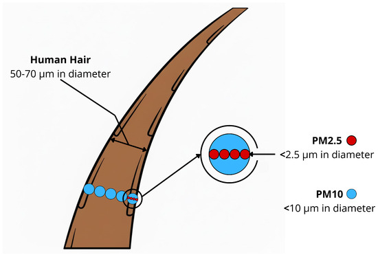
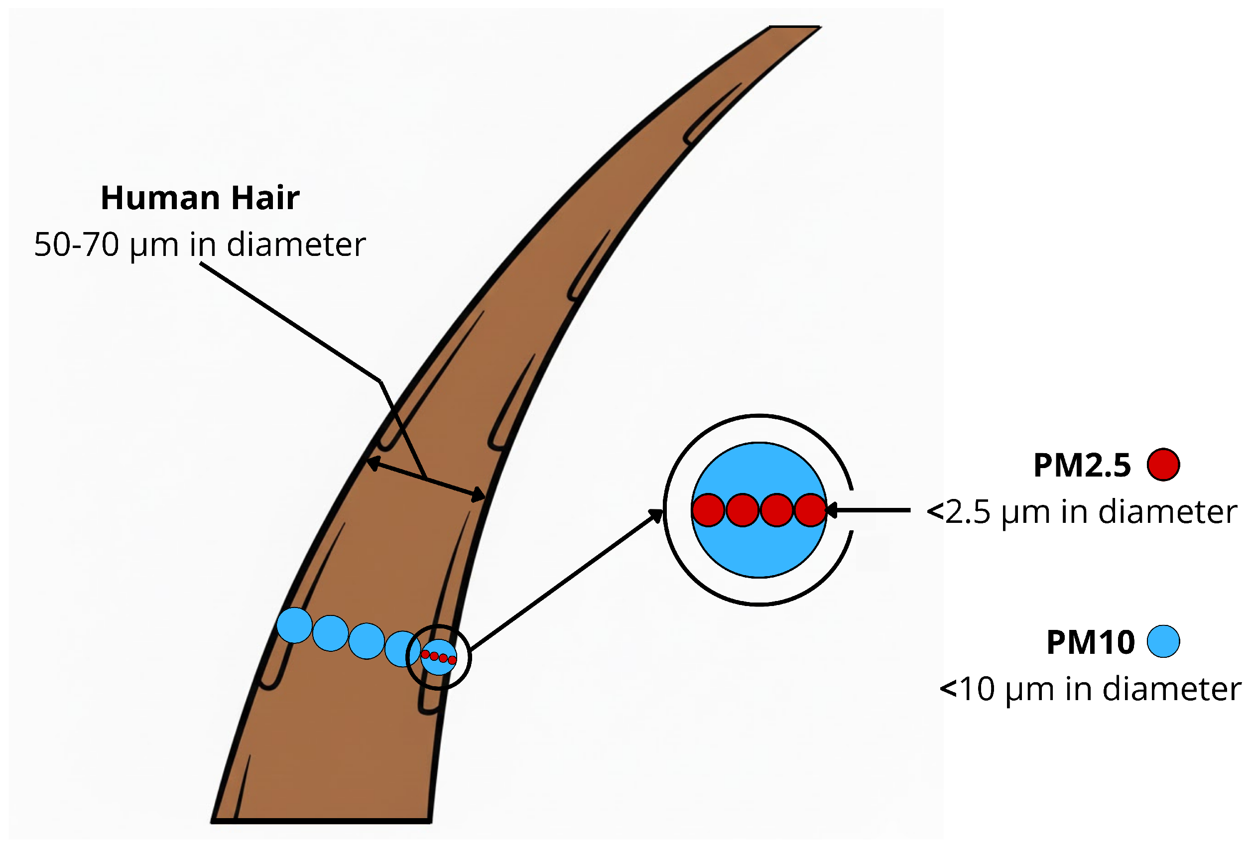
The high concentration of PM in the atmosphere causes several human health problems in multiple organ systems, including the respiratory, cardiovascular and central nervous systems [15]. Long-term exposure to PM is associated with lung cancer, and it is associated with decreased pulmonary function and many other health effects in humans [21]. Figure 1 shows the comparison size of PM particles.

Figure 1. Size comparisons for PM particles with a human hair. ${\mathrm{PM}}_{2.5}$ particles (red) and ${\mathrm{PM}}_{2.5}$ particles (blue).

In Mexico, the Mexican Official Standard (NOM), NOM-025-SSA1-2014, related to air quality levels, establishes the maximum average values for the concentration of particulate matter [22]. In a global context, the WHO also establishes the maximum acceptable average concentration levels of particulate matter [21]. These values are measured in $\mathsf{\mu }$g/m³ shown in Table 1.

Table 1. Overview of guidelines for particulate matter concentration levels according to WHO and NOM [21,22].

	PM10 (μg/m3)		PM2.5 (μg/m3)
	Daily Average	Annual Average	Daily Average	Annual Average
WHO	50	20	25	10
Mexico	75	40	45	12

2.2. Copulas

A copula is a powerful tool for modeling and capturing dependence structures among variables, mapping marginal distributions and forming their joint cumulative distribution [9]. Copulas were introduced in 1959 by Abe Sklar in order to pair random variables. Copulas have the ability to model the dependence structure independently from marginal distributions, allowing a better understanding of the dependence structure and a wide range of joint distributions [10,11].

A formal definition of a copula is as follows:

Definition 1 (Copula-definition). 

An n-dimensional copula is a function $C:{[0,1]}^n⟶[0,1]$, that satisfies the following properties:

• C is grounded, i.e., for every $\mathbf{u}=(u_1,\dots ,u_n)\in {[0,1]}^n$, $C\left(\mathbf{n}\right)=0$ if at least one coordinate is equals to zero.
• C grounded and increasing, i.e., the C-volume of every box whose vertices lie in ${[0,1]}^n$ is positive.
• $C(1,\dots ,1,u_i,1,\dots ,1)=u_i$ for all $u_i\in [0,1]$, $i=1,\dots ,n$.

Thus, a copula can be defined as a multivariate distribution supported on ${[0,1]}^n$ whose marginals are uniform on $[0,1]$ [8,11]. The most important concept in copula theory is Sklar’s Theorem 1.

Theorem 1 (Sklar’s Theorem). 

Given an n-dimensional distribution function F with continuous marginal distributions $F_1,\dots ,F_n$, then there exists an n-copula C such that.

$$F(x_1,\dots ,x_n)=C(F_1\left(x_1\right),\dots ,F_n\left(x_n\right))$$

(1)

Sklar’s theorem guarantees that the function C is unique if the marginal distributions $F_1,\dots ,F_n$ are continuous. This theorem provides both a construction scheme for copulas and a parametrization of multivariate distributions.

Given a multivariate distribution F with marginals $F_1,\dots ,F_n$ the function

$$C(u_1,\dots ,u_n)=F\left(F_1^{-1}\left(u_1\right),\dots ,F_n^{-1}\left(u_n\right)\right)$$

(2)

This automatically becomes a n-copula; this copula is the copula of the multivariate distribution F [8,11,23].

Gaussian Copulas

The Gaussian copula is the copula derived from the Gaussian distribution. Where $\mathsf{\Phi }$ is the cumulative distribution function of a normal distribution and ${\mathsf{\Phi }}_{\rho }$ is the n-dimensional joint cumulative distribution function of a multivariate normal distribution and $\rho$ is the correlation matrix [8].

$$C_{\rho }(u_1,\dots ,u_n)={\mathsf{\Phi }}_{\rho }\left({\mathsf{\Phi }}^{-1}\left(u_1\right),\dots ,{\mathsf{\Phi }}^{-1}\left(u_n\right)\right)$$

(3)

Whose density

$$c_{\rho }(u_1,\dots ,u_n)={\displaystyle \frac{\partial C_{\rho }(u_1,\dots ,u_n)}{\partial u_1,\dots ,\partial u_n}}$$

(4)

This can be described as:

$$c_{\rho }(u_1,\dots ,u_n)={\displaystyle \frac{1}{\sqrt{\det \rho }}}\exp \left(-{\displaystyle \frac{1}{2}}{\left[\begin{array}{c}{\mathsf{\Phi }}^{-1}\left(u_1\right)\\ ⋮\\ {\mathsf{\Phi }}^{-1}\left(u_n\right)\end{array}\right]}^{\mathsf{T}}\left({\rho }^{-1}-I\right)\left[\begin{array}{c}{\mathsf{\Phi }}^{-1}\left(u_1\right)\\ ⋮\\ {\mathsf{\Phi }}^{-1}\left(u_n\right)\end{array}\right]\right)$$

(5)

where ${\mathsf{\Phi }}^{-1}\left(u_i\right)$ is the inverse cumulative distribution function of a normal distribution [8].

Let us note that Theorem 1 and Equation (2) ensure that Equation (3) is a copula [8].

2.3. Neural Networks

The human brain possesses several advantages over a digital computer. Our brain is remarkably robust, and what makes it especially interesting is its ability to learn; it does not need any kind of upgrade. If we decide to learn something, the brain can adapt and make it possible [7].

The computations made by our brain are conducted by a highly interconnected network of neurons which communicate by sending electric pulses through the neural wiring consisting of axons, synapses and dendrites [7].

Artificial neural networks (ANNs) are inspired by the functionality of neurons in our brain. ANNs were developed to simulate the ability to learn using simple elements [4]. In 1943, Warren McCulloch and Walter Pitts modeled a neuron as a switch that receives input from other neurons and, depending on the total weighted input, is either activated or remains inactive, where the weight is the strength of the connection between neurons [7].

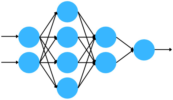
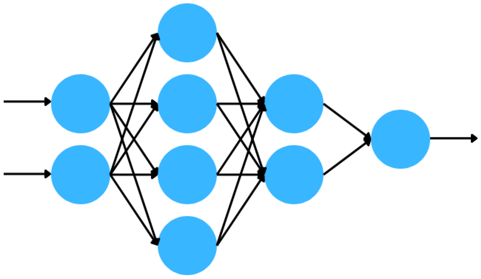
An ANN consists of three types of layers, the input layer, the hidden layers and the output layer. Where the input layer depends on the dimension of the data [24], and hidden layers are intermediate layers between the input and output layers. Some problems can be solved with a single hidden layer, while others require multiple hidden layers. The hidden layers are where training and feature learning take place [25]. Finally, the values obtained after the training came from the output layer; neurons in the output layer have a direct relation with the complexity of the problem [25].

In Figure 2, a basic illustration of a completely connected ANN.

Figure 2. Graphical illustration of a four-layer neural network with 2 inputs and 1 output, based on Ramírez-Montañez illustration.

Over the years, different ANN topologies have been proposed with different advantages and properties to solve different problems [4].

2.3.1. Recurrent Neural Networks

Recurrent Neural Networks (RNN), one of the most used and famous neural networks due to the capability to represent time series, video, audio or anything that is presented by means of data sequences [26]. RNNs embed historical input information in the network’s internal state and can map all historical input dates to obtain the final output [27].

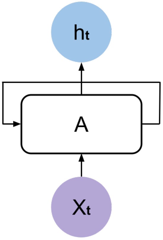
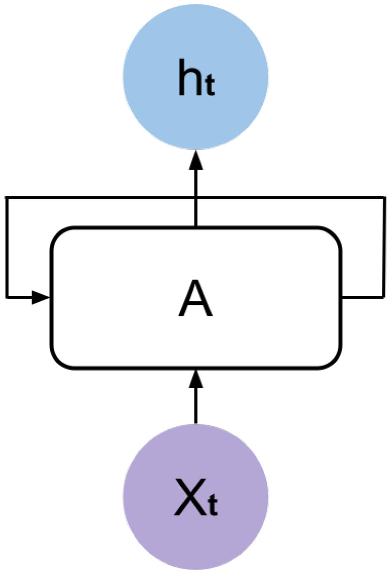
In Figure 3, where $x_t$ and $h_t$ are the input and output signals, respectively. This topology shows that RNNs are related to sequences and lists. In order to easily understand a simple RNN, we can think of an RNN as an NN with a single layer that is repeated and passes the information to the next NN. Usually, RNNs use the hyperbolic tangent activation function [5].

Figure 3. Recurrent neural network model.

2.3.2. LSTM Neural Network

The Long Short-Term Memory (LSTM) model, proposed by Hochreiter and Schmidhuber in 1997 [4]. They designed this model in order to avoid long-term dependency problems [27]. LSTM neural networks are capable of capturing data from past stages and using it for future predictions [24] by long-term memory in the form of weights [4], which are modified during network training and short-term memory defined in activation functions between the communication of the neuron nodes [7].

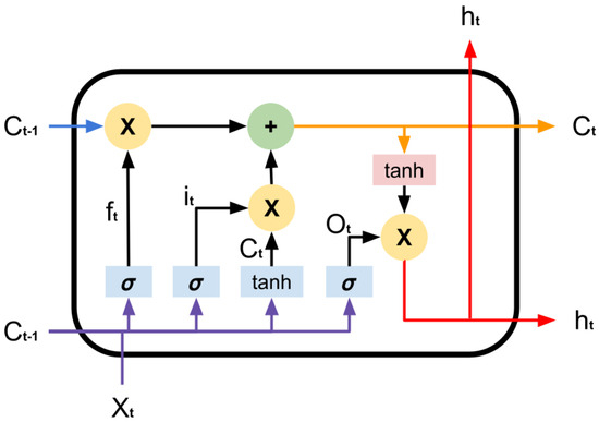
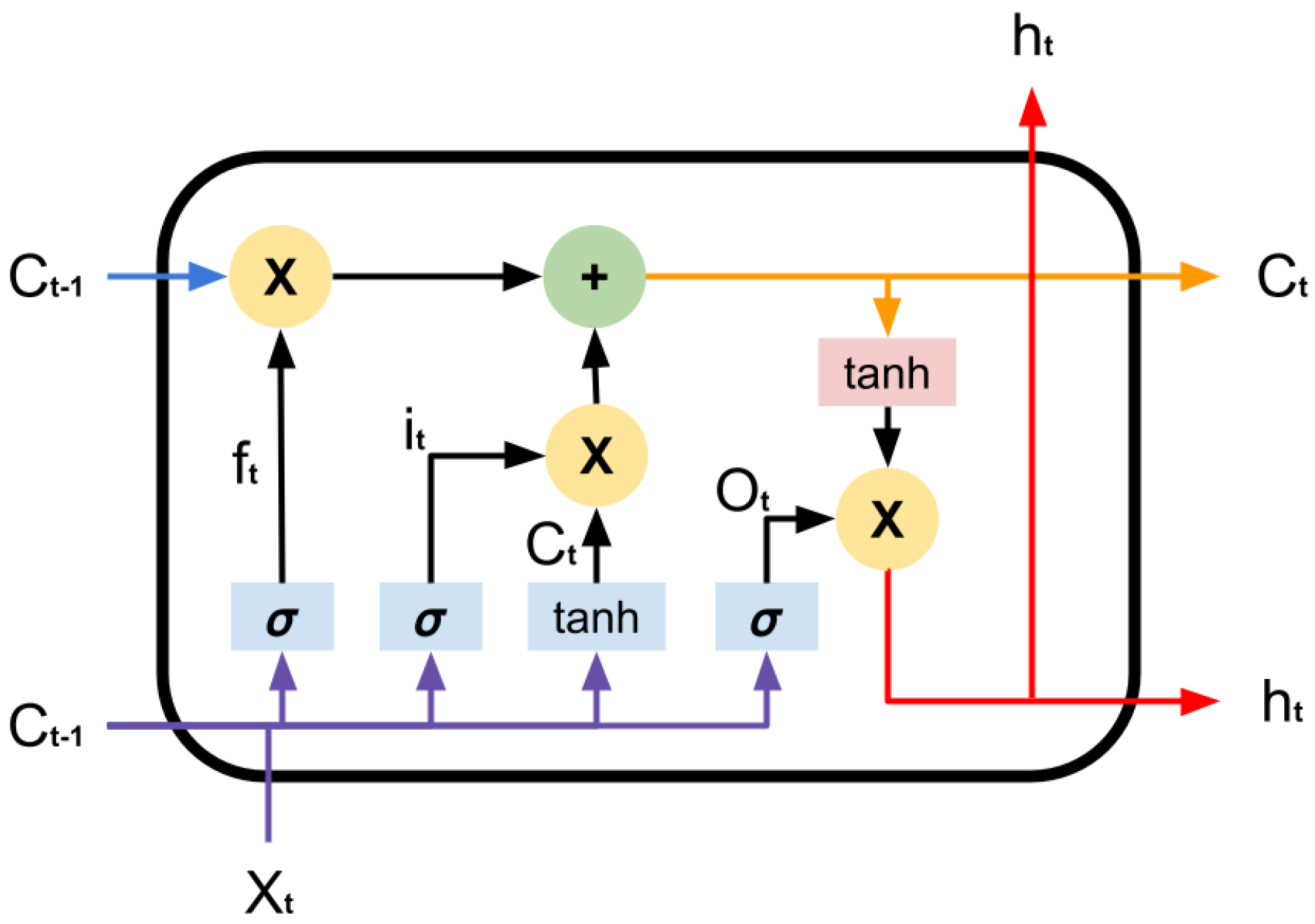
The LSTM model introduces a block of memory, composed by simple blocks connected in a specific way as in Figure 4 [4], this model has the capability to add or remove information to the cell state, regulated by structures called gates the input gate i, forget gate f and output gate o [5].

Figure 4. LSTM memory block where $f_t$ is the forget gate, $i_t$ the input gate and $O_t$ the output gate.

The LSTM model works as follows [5]:

1.

The forget gate takes the input values $h_{t-1}$ and $x_t$, then applies the sigmoid function $\sigma$ to determine what to preserve and discard. If the output of the sigmoid function is 1, the data needs to be kept entirely, while 0 erases the data, then it is multiplied by $C_{t-1}$.

$$f_t=\sigma \left(W·\left[h_{t-1},x_t\right]+b_f\right)$$

(6)

where W is the weight, $h_t$ is the hidden state and $b_f$ the bias.

2.

Then a sigmoid layer called input gate decides which values are going to be updated. Afterwards, a tanh layer creates a new vector of candidate values ${\widehat{C}}_t$, which could be added to the cell state. Then these two steps are combined to create an update to the state:

$$i_t=\sigma \left(W_i·\left[h_{t-1},x_t\right]+b_i\right)$$

(7)

$$C_t=tanh\left(W_c·\left[h_{t-1},x_t\right]+b_C\right)$$

(8)

3.

The next stage is that the old cell state $C_{t-1}$ is updated to the new cell state $C_t$.

$$C_t=f_t\ast C_{t-1}+i_t\ast C_t$$

(9)

4.

Finally, an output is chosen.

$$o_t=\sigma \left(W_o·\left[h_{t-1},x_t\right]+b_o\right)$$

(10)

$$h_t=o_t\ast tanh\left(C_t\right)$$

(11)

2.3.3. Neural Networks for Air Quality Research

Artificial neural networks have become important tools in air pollution research because of their ability to capture complex relationships among environmental variables. They have been applied to forecast different types of particulate matter and pollutants, improving the accuracy of air quality prediction compared to traditional methods.

Recent research by Mauricio-Alvarez et al. developed a transformer-based deep learning model to forecast coarse particulate matter (PMCO) levels at different forecasting horizons in Mexico City. The results demonstrated superior performance over conventional models across different prediction horizons [6].

A study conducted by Ramírez-Montañez et al. [4] employs a Long Short-Term Memory (LSTM) neural network to predict exceedances of ${\mathrm{PM}}_{10}$ particulate matter in Mexico City. The primary objective is to enhance air quality monitoring by forecasting instances when pollutant concentrations are expected to exceed the thresholds specified in the Mexican environmental standard NOM-025-SSA1-2014.

Becerra-Rico et al. developed a predictive model for airborne particulate pollution in Mexico City utilizing Long Short-Term Memory (LSTM) and Gated Recurrent Unit (GRU) architectures. The research aimed to forecast ${\mathrm{PM}}_{10}$ concentrations across various temporal horizons. Both models effectively captured the non-linear dynamics of particulate matter; LSTM generally yielded lower Root Mean Square Error (RMSE) values for short-term predictions, whereas GRU produced more consistent performance over extended forecast periods [5].

In other works related to the prediction of the levels of particulate matter, the authors Zhiyuan et al. combined 6 machine learning algorithms for the prediction of ${\mathrm{PM}}_{2.5}$ and NO_X particles at three roadside stations in Hong Kong [28].

These examples show how neural networks are becoming valuable tools for air pollution research, helping to improve predictions and support better air quality management.

3. Materials and Methods

Mexico has a monitoring network in Mexico City named the Atmospheric Monitoring System (SIMAT). This system is responsible for monitoring air quality. It is complemented by four subsystems: the Automatic Atmospheric Monitoring Network (RAMA), Manual Atmospheric Monitoring Network (REDMA), Meteorology and Solar Radiation Network (REDMET) and Deposit Atmospheric Network (REDDA) [3].

The RAMA network uses equipment to measure carbon dioxide, carbon monoxide, nitrogen dioxide, ozone, nitrogen oxides, sulfur dioxide, ${\mathrm{PM}}_{10}$, ${\mathrm{PM}}_{2.5}$ and coarse particles [3].

The time series variables used to train and test the model are ${\mathrm{PM}}_{10}$ and ${\mathrm{PM}}_{2.5}$ particle pollution concentrations in $\mathsf{\mu }$g/m³.

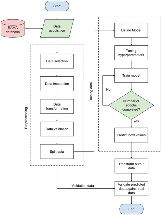
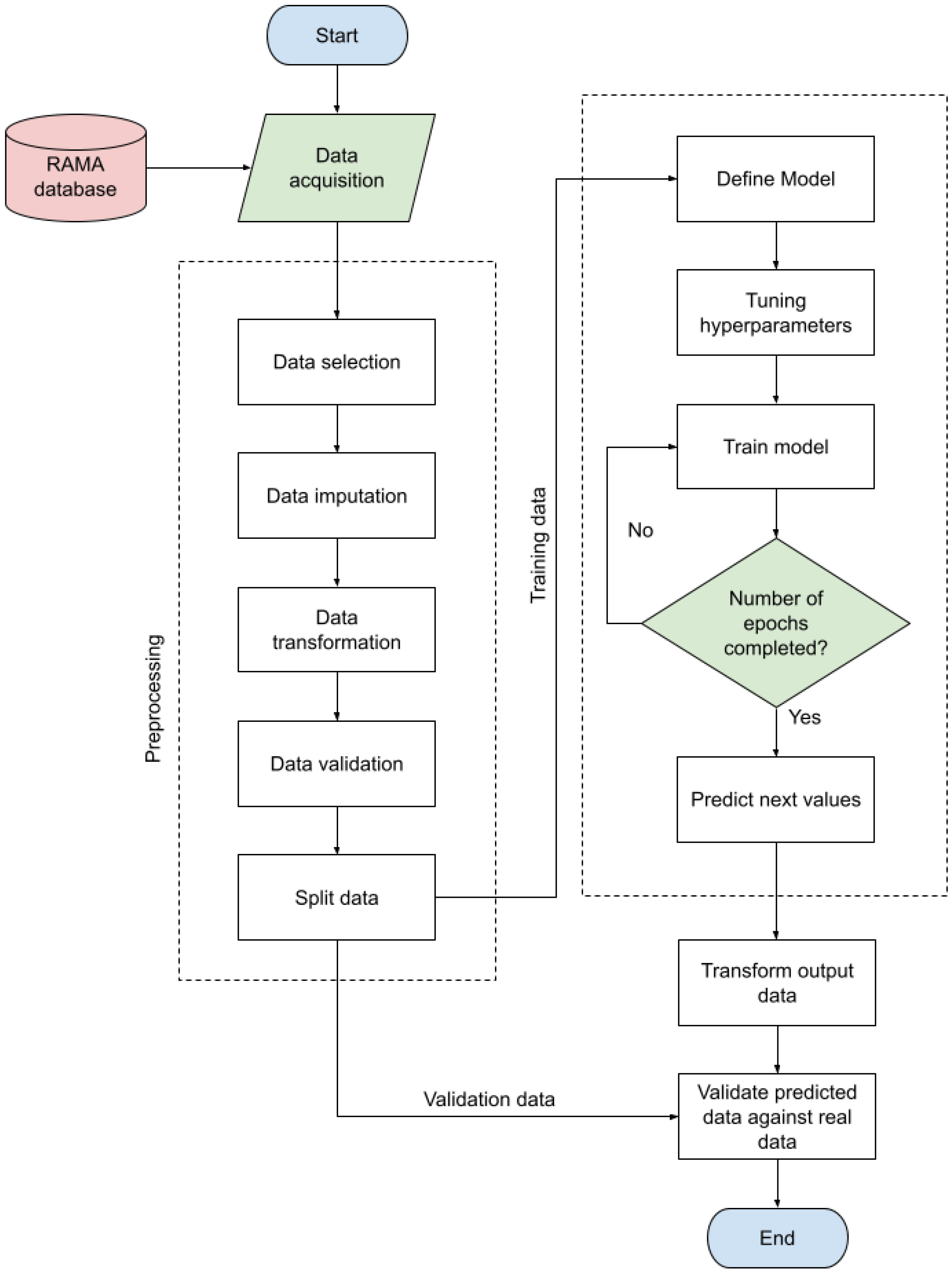
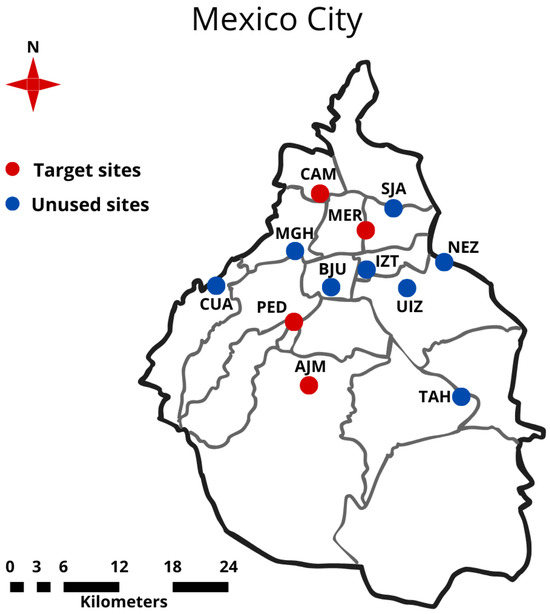
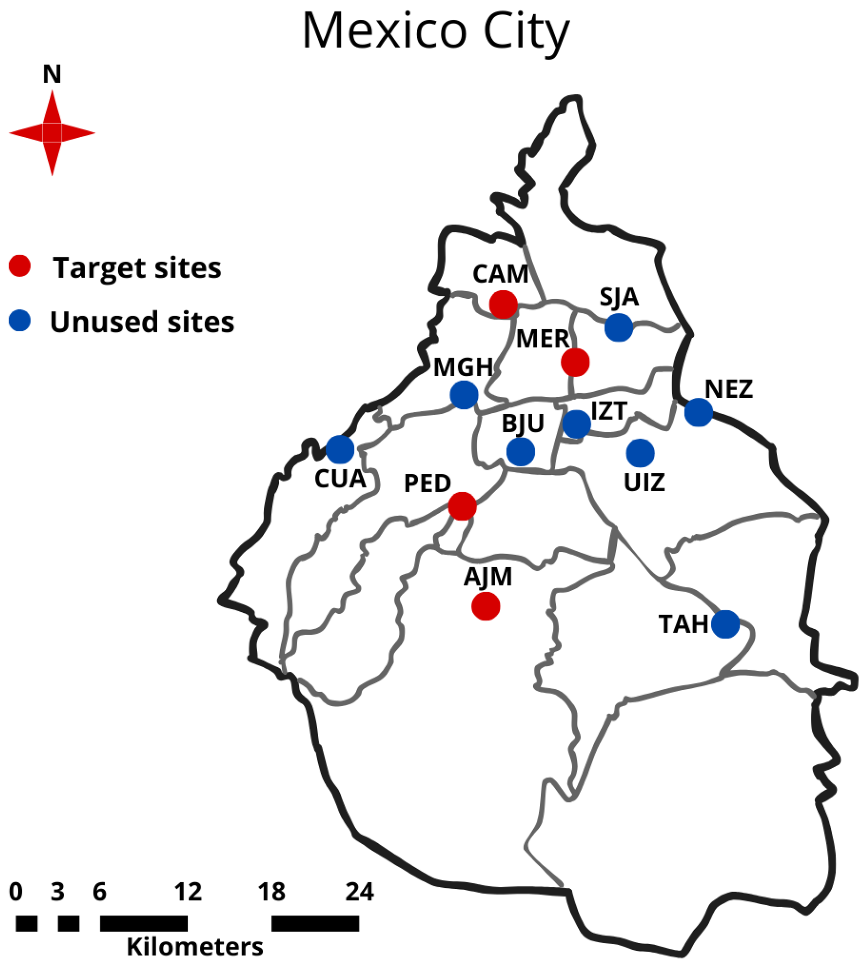
The following methodology was based on an investigation previously mentioned by Mauricio-Alvarez [6]. The next methodology Figure 5 was followed for ${\mathrm{PM}}_{10}$ and ${\mathrm{PM}}_{2.5}$ airborne particle forecasting using as training data the AJM (Ajusco Medio), CAM (Camarones), MER (Merced) and PED (Pedregal) stations Figure 6.

Figure 5. Methodology flowchart.

Figure 6. Geographic location of the monitoring stations networks, AJM, CAM, MER and PED stations (red color).

1.

Data acquisition: the raw data used was obtained from RAMA since January 2024 to December 2024, specifically the ${\mathrm{PM}}_{10}$ and ${\mathrm{PM}}_{2.5}$ data were obtained from the RAMA database.

2.

Data selection: This segment involves the selection of monitoring stations exhibiting the minimum percentage of missing values across all examined variables. For this study, the stations AJM, CAM, MER, and PED (Figure 6) within the Mexico City metropolitan area were selected. Table 2 presents the percentage of missing values for each variable. (Figure 6)

Table 2. Percentage of missing values for ${\mathrm{PM}}_{10}$ and ${\mathrm{PM}}_{2.5}$ at AJM, CAM, MER and PED stations.

	AJM	CAM	MER	PED
${\mathrm{PM}}_{10}$	7.69%	16.07%	12.90%	10.32%
${\mathrm{PM}}_{2.5}$	8.44%	16.85%	13.22%	10.87%

3.

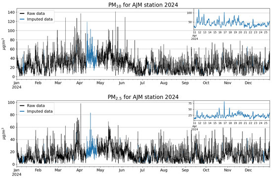
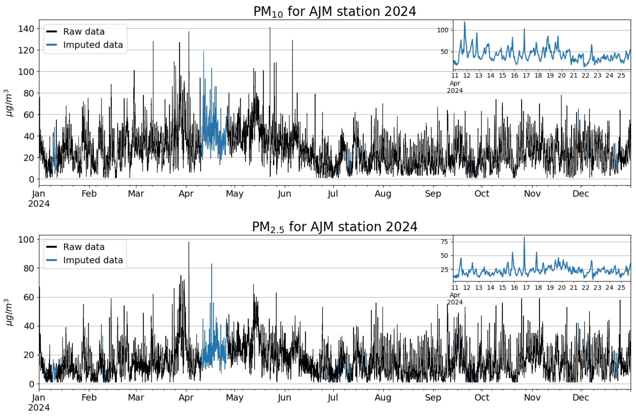
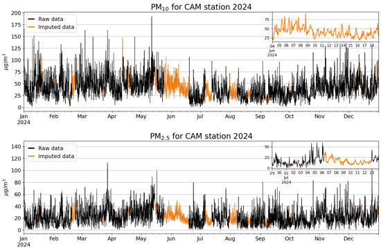
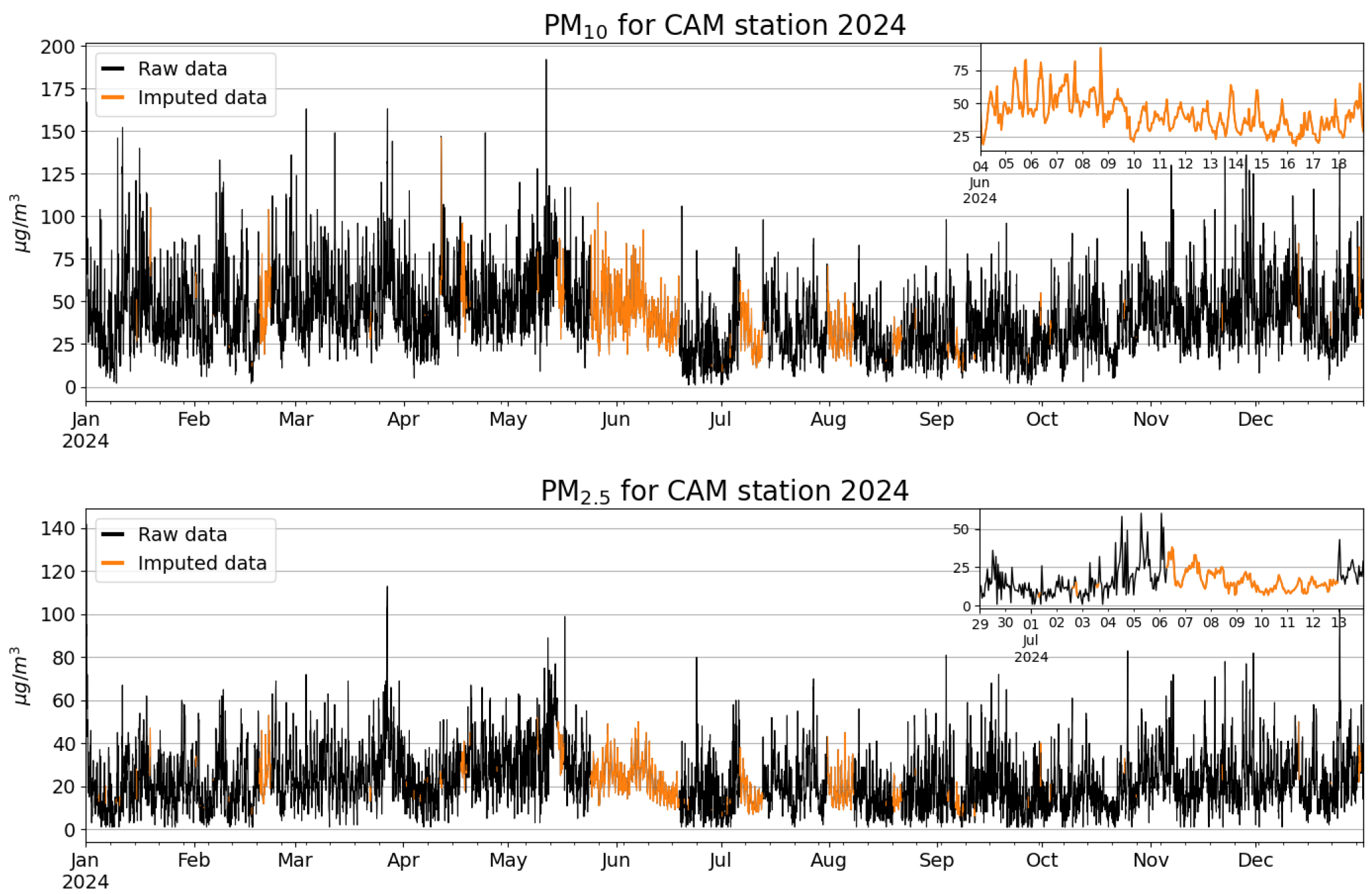
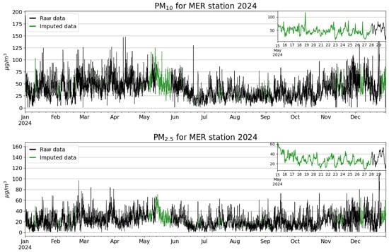
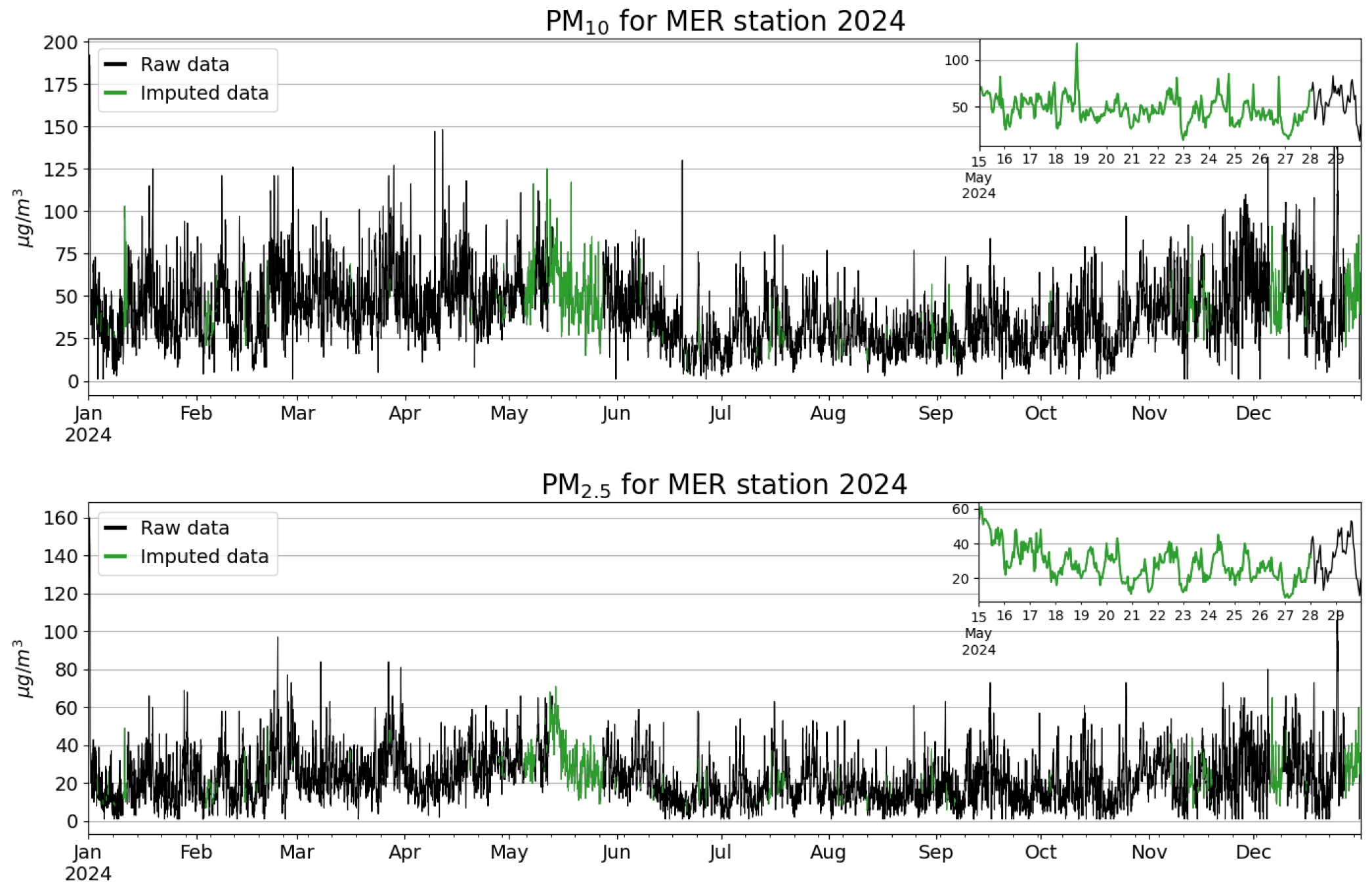
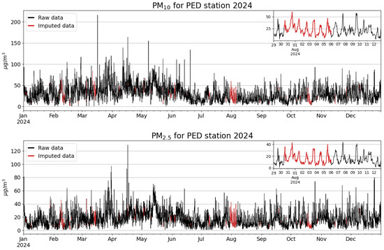
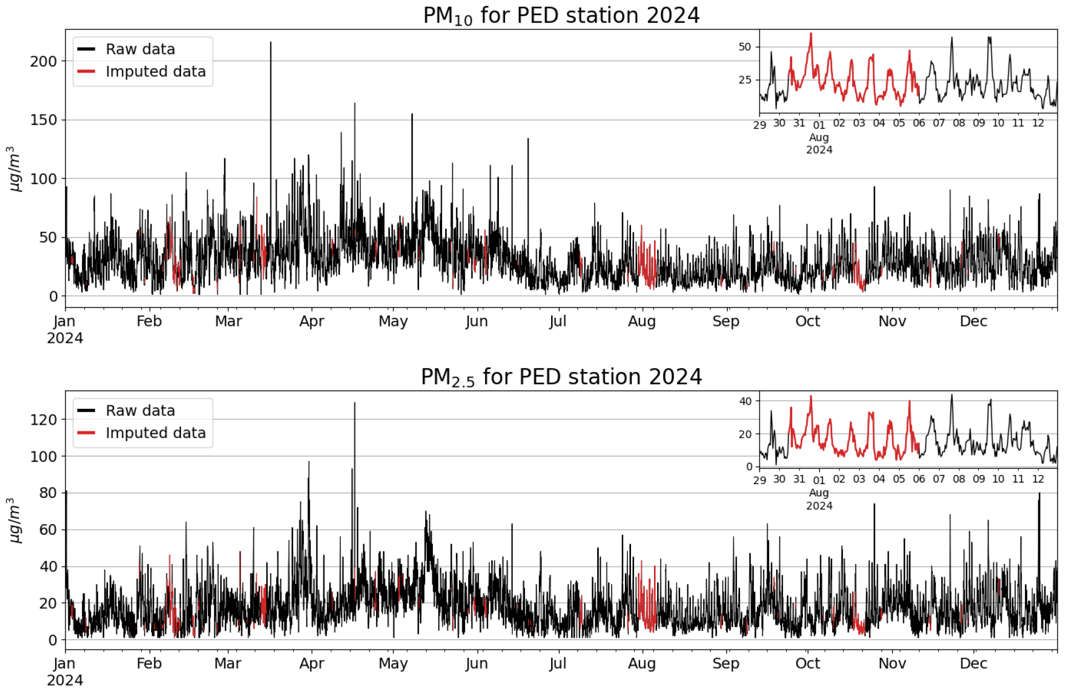
Fill missing values: The MICE (Multivariate Imputation by Chained Equations) technique was selected to handle missing data. In Figure 7, Figure 8, Figure 9 and Figure 10, it is observed that the ${\mathrm{PM}}_{10}$ and ${\mathrm{PM}}_{2.5}$ raw data and imputed data for AJM, CAM, MER and PED stations, respectively.

Figure 7. Raw data (shown in black) and imputed data (blue color) for ${\mathrm{PM}}_{10}$ and ${\mathrm{PM}}_{2.5}$ particle levels at AJM station.

Figure 8. Raw data (showed in black) and imputed data (orange color) for ${\mathrm{PM}}_{10}$ and ${\mathrm{PM}}_{2.5}$ particles levels at CAM station.

Figure 9. Raw data (showed in black) and imputed data (green color) for ${\mathrm{PM}}_{10}$ and ${\mathrm{PM}}_{2.5}$ particles levels at MER station.

Figure 10. Raw data (shown in black) and imputed data (red color) for ${\mathrm{PM}}_{10}$ and ${\mathrm{PM}}_{2.5}$ particle levels at PED station.

4.

Data transformation: Box–Cox function was used to transform the original data distribution to a better approximation of a normal distribution.

5.

Data segmentation: The dataset used includes the 366 days of the year 2024. The data will be divided into 6 subsets, each subset represents two months of the year 2024, January-February, March-April, May-June, July-August, September-October and November-December. All the subsets will be separated into training (80%) and testing (20%). This separation will help reduce overfitting, thus ensuring the accuracy of the results.

6.

Model construction: For forecasting purposes, the LSTM model was selected due to its proficiency in capturing temporal dependencies within time series data, augmented by enhancements to the loss function incorporating Gaussian copulas.

The proposed novel loss function is as follows.

$$\mathrm{Loss}\mathrm{Function}=\mathrm{MSE}-\mathrm{Gaussian}\mathrm{Copula}\mathrm{Density}\mathrm{Function}$$

(12)

MSE is the Mean Squared Error given by

$$\mathrm{MSE}={\displaystyle \frac{1}{N}}\sum _{i=0}^N\left(y_i-\widehat{y_i}\right)$$

(13)

where $y_i$ is the real value and $\widehat{y_i}$ is the predicted value

$$\mathrm{Loss}\mathrm{function}={\displaystyle \frac{1}{N}}\sum _{i=0}^N\left(y_i-\widehat{y_i}\right)-\lambda ·c_{\rho }\left(\widehat{y}\right)$$

(14)

A better description of $c_{\rho }\left(\widehat{y}\right)$ is given by

$$c_{\rho }({\widehat{y}}_1,\dots ,{\widehat{y}}_N)={\displaystyle \frac{1}{\sqrt{\det \rho }}}\exp \left(-{\displaystyle \frac{1}{2}}{\left[\begin{array}{c}{\mathsf{\Phi }}^{-1}\left({\widehat{y}}_1\right)\\ ⋮\\ {\mathsf{\Phi }}^{-1}\left({\widehat{y}}_N\right)\end{array}\right]}^{\mathsf{T}}\left({\rho }^{-1}-I\right)\left[\begin{array}{c}{\mathsf{\Phi }}^{-1}\left({\widehat{y}}_1\right)\\ ⋮\\ {\mathsf{\Phi }}^{-1}\left({\widehat{y}}_N\right)\end{array}\right]\right)$$

(15)

$\lambda$ is a constant to regulate the weight of the Gaussian copula density term.

7.

Comparative model: The model used to compare the time series is the same as an LSTM neural network with the same hyperparameters; the difference is the loss function, which is MSE.

8.

Model training: The LSTM neural network was trained using the training dataset with the hyperparameters shown in Table 3. The model has a key difference in a new proposed loss function.

Table 3. LSTM model hyperparameters.

Hyperparameter	Value
Input Shape	loop_back,2
Loop back	24
Learning rate	0.001
LSTM Units	64
Optimizer	Adam
Loss Function	MSE $-\lambda ·$ Gaussian Copula Density or MSE
Epochs	20
Batch Size	32

9.

Forecasting for evaluation: After training, the model for LSTM with data augmentation dataset and the original dataset were both used to predict future values of 12, 24, 48 and 72 h intervals. To validate the performance of the model with and without data augmentation, we used multiple evaluation metrics: Root Mean Square Error (RMSE), Mean Absolute Error (MAE) and Mean Absolute Percentage Error (MAPE). These metrics indicate if there is an improvement of the model performance.

3.1. Missing Values Imputation

In order to fill the missing values in our original dataset, the technique implemented is MICE (Multivariate Imputation by Chained Equations). Table 4 and Table 5 show the statistical values for the raw dataset and the imputed dataset, respectively.

Table 4. Raw data statistics for ${\mathrm{PM}}_{10}$ and ${\mathrm{PM}}_{2.5}$ particles.

	PM2 (μg/m3)					PM2.5 (μg/m3)
Station	Min	Max	Mean	$\mathbf{\sigma }$	Missing Values	Min	Max	Mean	$\mathbf{\sigma }$	Missing Values
AJM	1.0	141	26.165	16.052	674	1.0	98	15.916	11.005	739
CAM	1.0	192	42.050	21.769	1412	1.0	142	22.838	13.545	1480
MER	1.0	192	40.271	20.753	1130	1.0	160	22.649	13.751	1158
PED	1.0	216	30.786	17.898	904	1.0	129	18.002	11.438	952

Table 5. Imputed data statistics for ${\mathrm{PM}}_{10}$ and ${\mathrm{PM}}_{2.5}$ particles.

	PM10 (μg/m3)				PM2.5 (μg/m3)
Station	Min	Max	Mean	$\mathbf{\sigma }$	Min	Max	Mean	$\mathbf{\sigma }$
AJM	1.0	141	26.693	16.268	1.0	98	16.034	10.925
CAM	1.0	142	41.708	21.087	1.0	142	22.612	12.910
MER	1.0	192	40.989	20.368	1.0	160	23.368	13.512
PED	1.0	216	30.413	17.616	1.0	129	17.690	11.228

3.2. Data Transformation

Gaussian copulas have the characteristic of dealing with normal distribution data and use the normal distribution as an intermediate distribution to model complex joint probability distributions [29].

As mentioned before, the data might follow a normal distribution. In this investigation, none of the data implemented follows a normal distribution according to the Anderson–Darling hypothesis test [30]. This test was selected due to an investigation conducted by Scholz [31], who mentioned in his research that this test is one of the most powerful among other tests.

Table 6 shows the statistical value for the Anderson–Darling hypothesis test, where none of the variables for each station follow a normal distribution.

Table 6. Statistic value of Anderson–Darling hypothesis test for ${\mathrm{PM}}_{10}$ and ${\mathrm{PM}}_{2.5}$ for AJM, CAM, MER and PED stations.

Variable	AJM	CAM	MER	PED
${\mathrm{PM}}_{10}$	3.076	6.155	4.168	4.106
${\mathrm{PM}}_{2.5}$	6.155	4.877	8.654	8.038

In this case, the use of Gaussian copulas is not the best option due to the data distribution based on the results of Table 6, but fortunately, the Box–Cox function helped with this [32], which is used to transform the data distribution to a normal distribution. Box and Cox introduced a power transformation, which is given by:

$$y^{\left(\lambda \right)}=\left\{\begin{array}{ccc}(y^{\lambda }-1)/\lambda & & \lambda \ne 0\\ lny& & \lambda =0\end{array}\right.$$

(16)

where $\lambda \in \mathbb{R}$ is the power transformation parameter.

Table 7 shows the result of the Anderson–Darling hypothesis test used for data transformed by the Box–Cox function.

Table 7. Results of Anderson–Darling hypothesis test for ${\mathrm{PM}}_{10}$ and ${\mathrm{PM}}_{2.5}$ variables transformed by Box–Cox function at AJM, CAM, MER and PED stations.

Variable	AJM	CAM	MER	PED
${\mathrm{PM}}_{10}$	0.619	0.366	0.253	0.746
${\mathrm{PM}}_{2.5}$	0.631	0.566	0.589	0.448

The outcomes derived from the Anderson–Darling normality test revealed that the Box–Cox function emerges as an optimal data transformation. Table 8 shows the statistics for transformed data. After this transformation, Gaussian copulas can be an option for these data.

Table 8. Transformed data statistics for ${\mathrm{PM}}_{10}$ and ${\mathrm{PM}}_{2.5}$ particles.

	PM10				PM2.5
Station	Min	Max	Mean	$\mathbf{\sigma }$	Min	Max	Mean	$\mathbf{\sigma }$
AJM	0.0	16.995	6.714	2.521	0.0	12.084	4.425	1.950
CAM	0.0	17.231	8.046	2.148	0.0	16.862	6.121	2.134
MER	0.0	21.467	9.230	2.659	0.0	17.000	6.015	2.091
PED	0.0	14.667	5.937	1.767	0.0	11.364	4.309	1.541

3.3. Forecasting

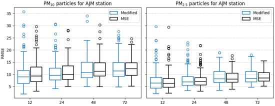
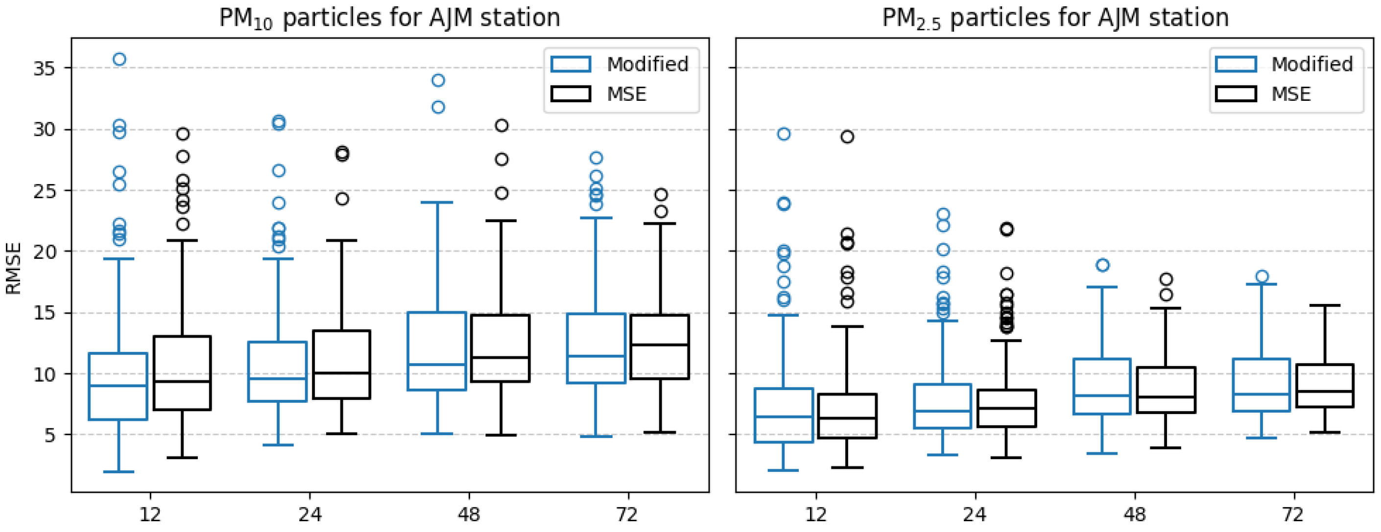
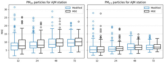
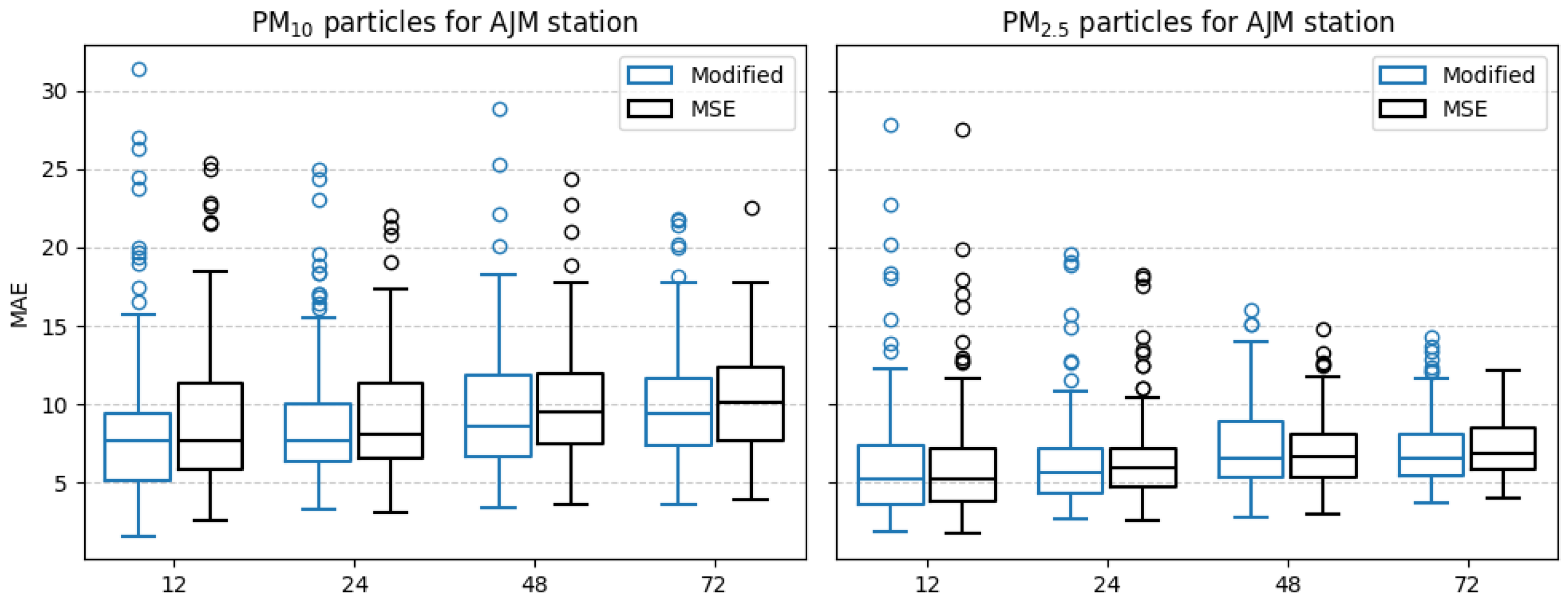
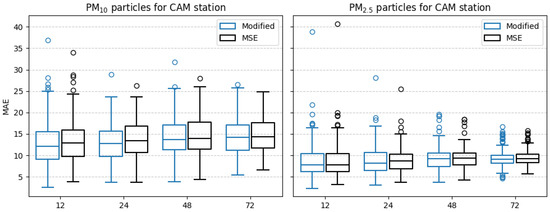
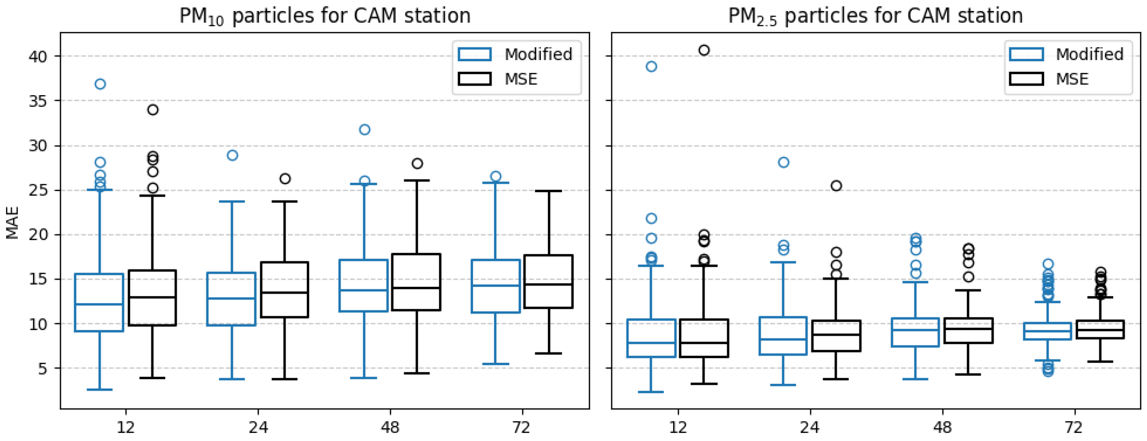
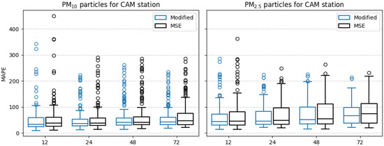
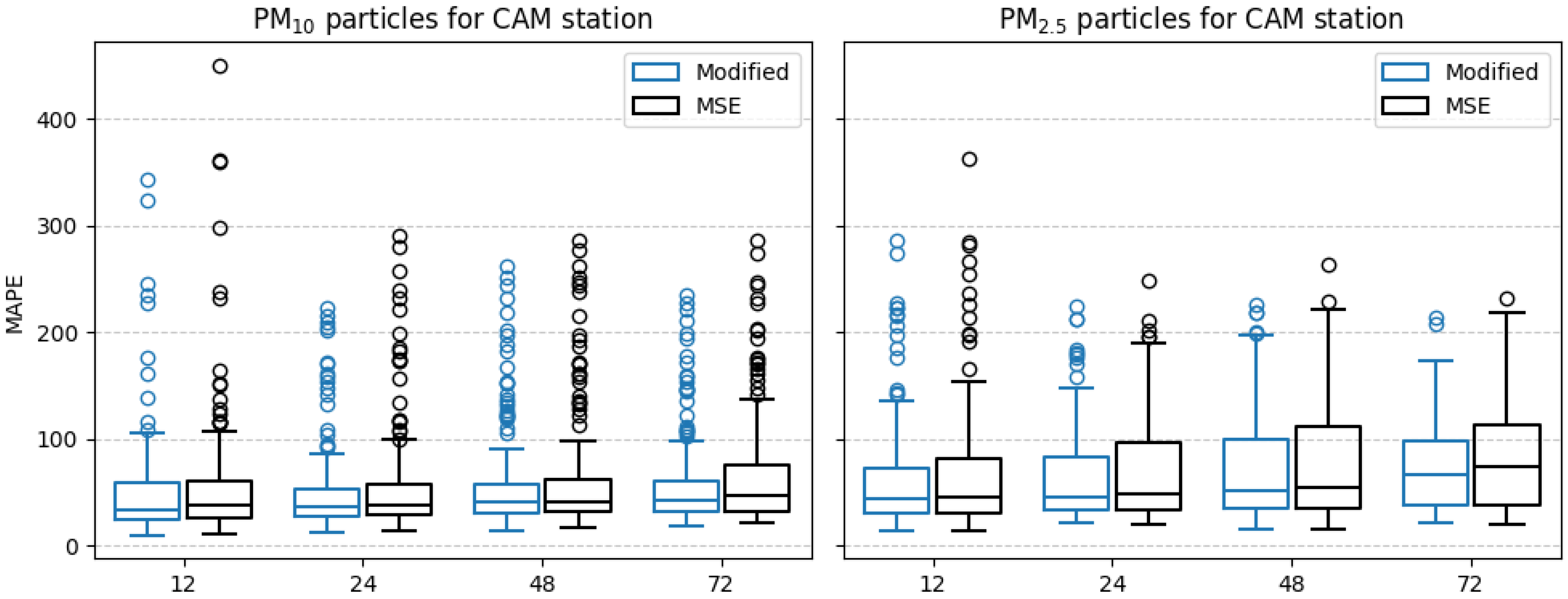
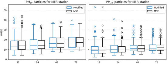
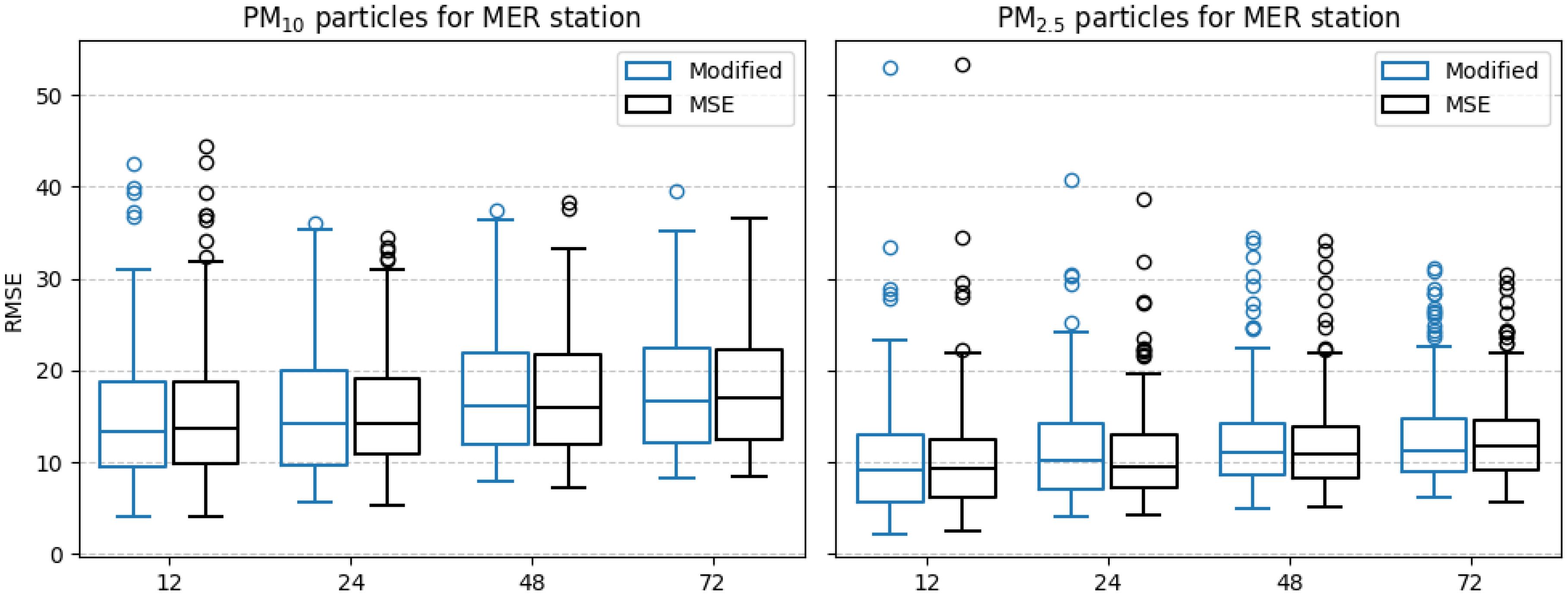
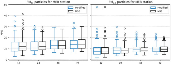
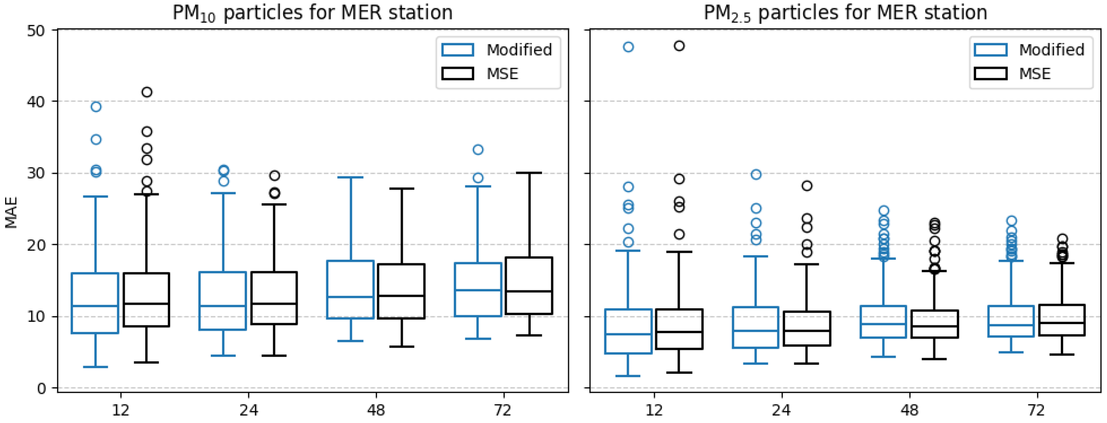
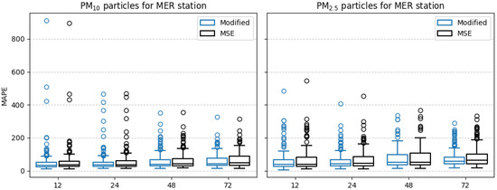
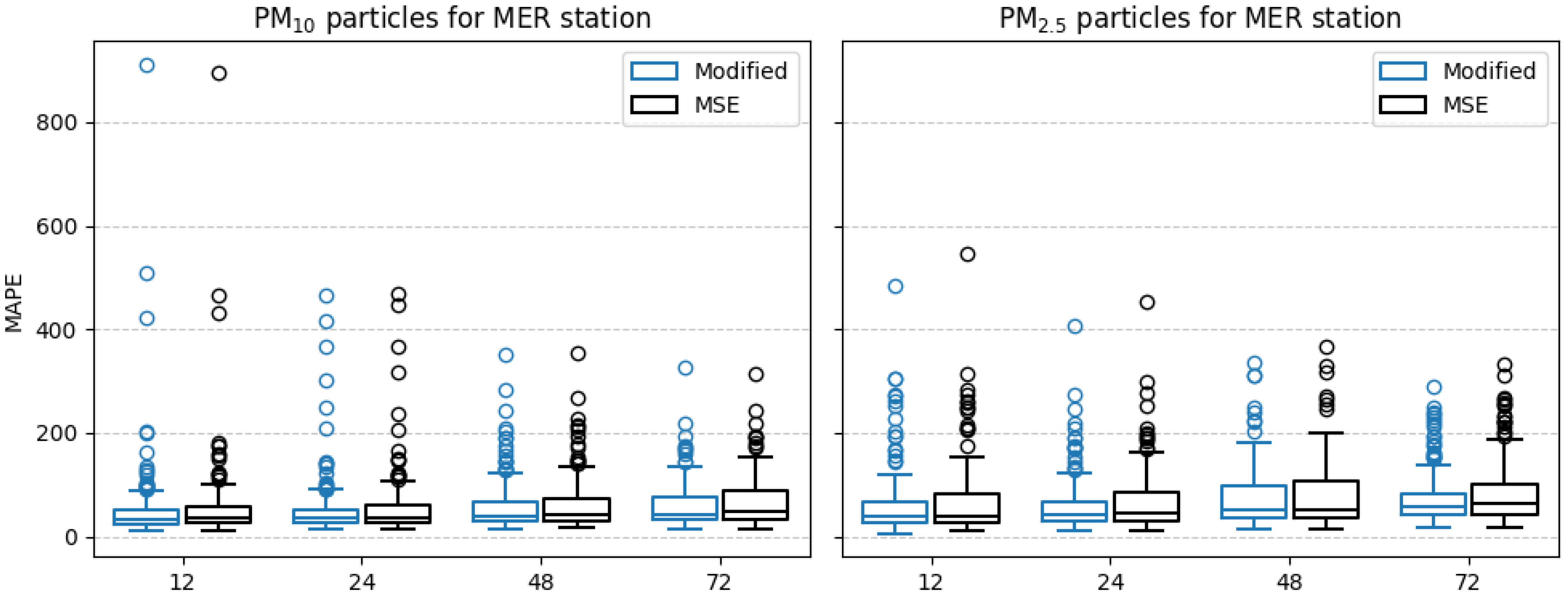
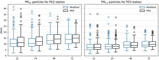
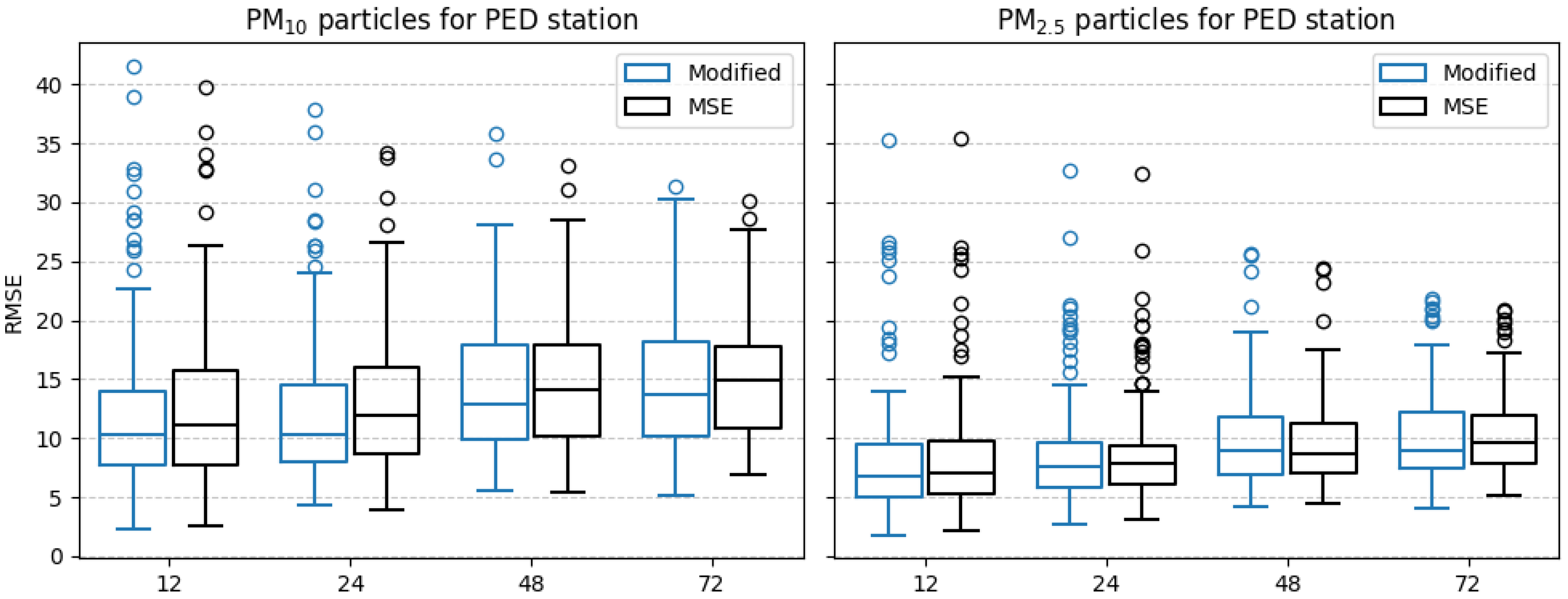
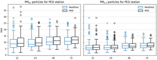
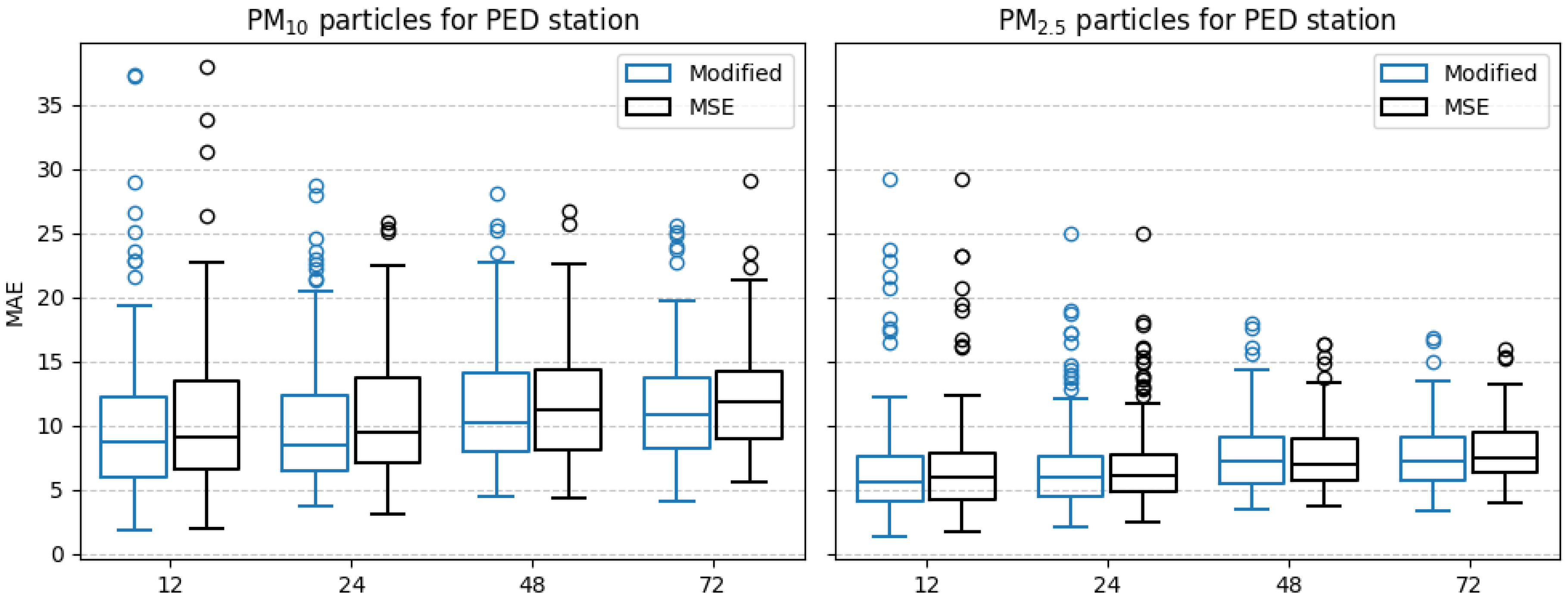
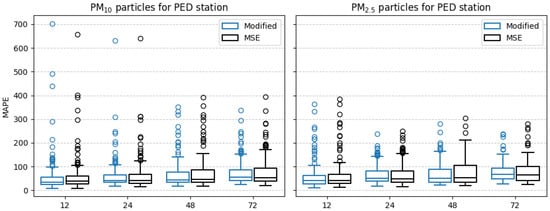
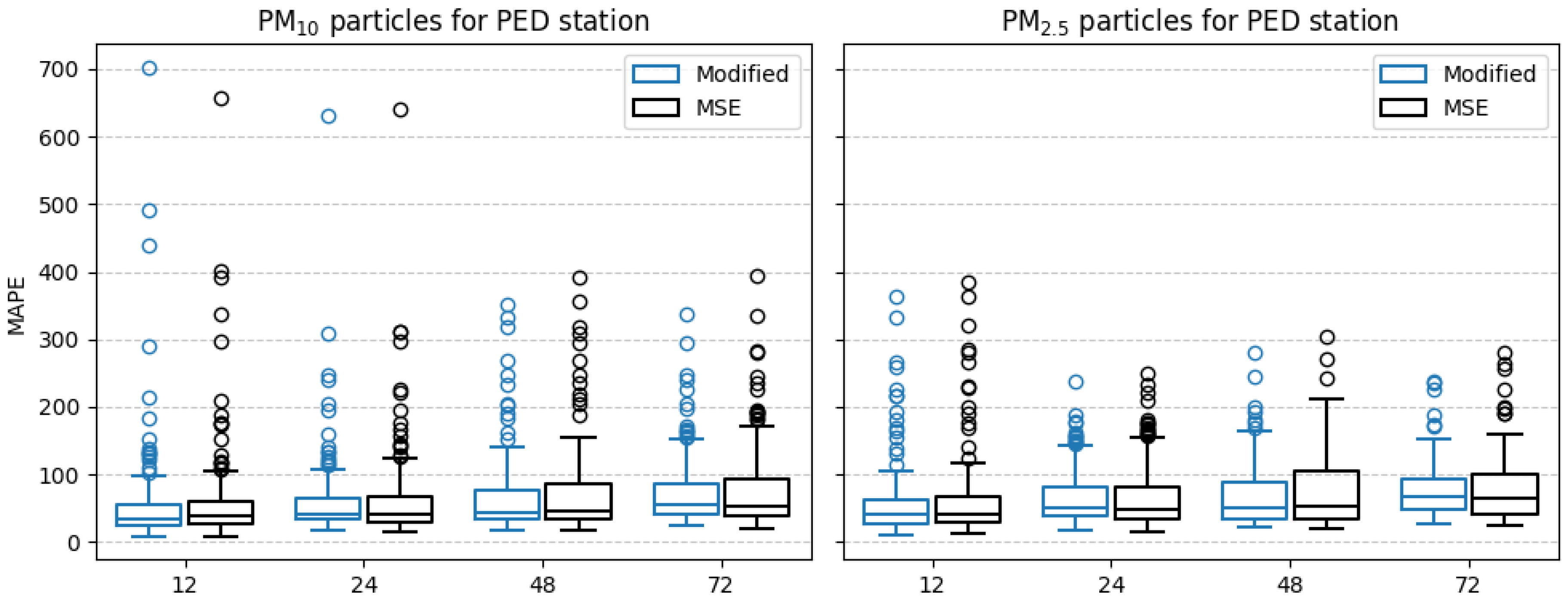
The results of the models’ performance LSTM with a modified loss function and LSTM model for forecasting ${\mathrm{PM}}_{10}$ and ${\mathrm{PM}}_{2.5}$ at AJM, CAM, MER and PED stations are presented in the following Table 9, Table 10, Table 11, Table 12, Table 13, Table 14, Table 15, Table 16, Table 17, Table 18, Table 19 and Table 20 show the minimum, maximum and mean values for the error metrics described before. In addition, Figure 11, Figure 12, Figure 13, Figure 14, Figure 15, Figure 16, Figure 17, Figure 18, Figure 19, Figure 20, Figure 21 and Figure 22 show boxplots of the error metrics for different forecast horizons using the modified loss function and MSE as the loss function.

Table 9. LSTM with modified loss function RMSE (μg/m³) ${\mathrm{PM}}_{10}$.

Hours	12			24			48			72
Site	Min	Max	Mean	Min	Max	Mean	Min	Max	Mean	Min	Max	Mean
AJM	1.979	35.743	10.068	4.173	30.710	10.786	5.004	33.976	12.198	4.855	27.617	12.564
CAM	3.175	39.222	15.770	4.673	36.464	16.331	4.937	39.626	17.999	6.804	34.072	18.157
MER	4.072	42.559	14.964	5.616	36.036	15.624	7.916	37.407	17.393	8.220	39.576	17.897
PED	2.291	41.542	12.049	4.345	37.920	12.682	5.624	35.838	14.280	5.196	31.347	14.649

Table 10. LSTM with modified loss function MAE (μg/m³) ${\mathrm{PM}}_{10}$.

Hours	12			24			48			72
Site	Min	Max	Mean	Min	Max	Mean	Min	Max	Mean	Min	Max	Mean
AJM	1.583	31.417	8.467	3.250	24.958	8.828	3.417	28.896	9.886	3.542	21.847	10.060
CAM	2.583	36.833	13.091	3.750	28.875	13.111	3.833	31.729	14.461	5.486	26.486	14.450
MER	2.917	39.250	12.660	4.458	30.500	12.691	6.458	29.375	14.037	6.875	33.333	14.262
PED	1.833	37.333	10.065	3.792	28.750	10.208	4.500	28.167	11.413	4.139	25.667	11.590

Table 11. LSTM with modified loss function MAPE (%) ${\mathrm{PM}}_{10}$.

Hours	12			24			48			72
Site	Min	Max	Mean	Min	Max	Mean	Min	Max	Mean	Min	Max	Mean
AJM	10.34	504.66	63.83	11.45	436.67	68.33	15.14	588.30	84.63	17.78	567.03	84.35
CAM	10.27	342.76	51.26	13.25	223.64	51.91	14.19	261.28	61.70	19.23	234.92	61.55
MER	11.72	911.22	57.05	15.07	466.85	55.80	14.33	352.58	62.36	14.17	326.80	61.45
PED	9.15	702.43	57.33	16.51	630.08	63.51	16.47	351.74	66.91	23.87	338.53	76.07

Table 12. LSTM with modified loss function RMSE (μg/m³) ${\mathrm{PM}}_{2.5}$.

Hours	12			24			48			72
Site	Min	Max	Mean	Min	Max	Mean	Min	Max	Mean	Min	Max	Mean
AJM	2.082	29.628	7.395	3.335	23.059	7.808	3.388	18.893	8.990	4.754	18.021	9.082
CAM	2.887	44.373	10.548	3.791	37.129	11.113	4.477	28.941	11.900	5.278	24.138	12.159
MER	2.236	53.088	10.396	4.031	40.717	11.411	4.914	34.519	12.485	6.242	31.146	12.892
PED	1.803	35.338	8.202	2.723	32.731	8.689	4.240	25.681	9.958	4.064	21.917	10.147

Table 13. LSTM with modified loss function MAE (μg/m³) ${\mathrm{PM}}_{2.5}$.

Hours	12			24			48			72
Site	Min	Max	Mean	Min	Max	Mean	Min	Max	Mean	Min	Max	Mean
AJM	1.833	27.833	6.158	2.625	19.625	6.297	2.771	16.000	7.147	3.736	14.319	7.065
CAM	2.333	38.833	8.702	3.042	28.125	8.849	3.792	19.625	9.345	4.611	16.667	9.340
MER	1.667	47.667	8.763	3.333	29.833	9.080	4.271	24.792	9.820	4.903	23.319	9.957
PED	1.417	29.250	6.809	2.167	25.042	6.934	3.438	17.938	7.803	3.347	16.833	7.801

Table 14. LSTM with modified loss function MAPE (%) ${\mathrm{PM}}_{2.5}$.

Hours	12			24			48			72
Site	Min	Max	Mean	Min	Max	Mean	Min	Max	Mean	Min	Max	Mean
AJM	11.79	390.27	64.06	12.47	264.93	69.54	18.90	308.79	81.31	21.66	273.38	81.35
CAM	13.96	286.45	64.68	21.57	223.99	64.87	15.47	225.96	73.87	22.06	214.62	73.52
MER	6.24	484.09	63.68	12.37	408.09	62.87	15.75	334.78	75.87	17.19	289.81	77.08
PED	10.53	363.41	58.47	16.71	238.13	66.61	21.40	280.75	68.02	27.59	238.46	77.60

Table 15. LSTM RMSE (μg/m³) ${\mathrm{PM}}_{10}$.

Hours	12			24			48			72
Site	Min	Max	Mean	Min	Max	Mean	Min	Max	Mean	Min	Max	Mean
AJM	3.052	29.590	10.390	5.067	28.104	11.134	4.954	30.344	12.284	5.161	24.620	12.678
CAM	5.061	37.210	16.110	4.428	33.951	16.767	5.234	36.098	18.107	8.265	31.255	18.553
MER	4.114	44.479	15.362	5.355	34.544	15.738	7.239	38.262	17.263	8.452	36.670	18.184
PED	2.598	39.840	12.535	3.951	34.271	13.155	5.353	33.134	14.352	6.936	30.189	15.023

Table 16. LSTM MAE (μg/m³) ${\mathrm{PM}}_{10}$.

Hours	12			24			48			72
Site	Min	Max	Mean	Min	Max	Mean	Min	Max	Mean	Min	Max	Mean
AJM	2.516	25.367	8.807	3.081	22.084	9.220	3.555	24.394	10.129	3.903	22.523	10.301
CAM	3.881	33.984	13.504	3.732	26.234	13.706	4.387	28.015	14.728	6.623	24.796	15.059
MER	3.459	41.358	13.056	4.450	29.711	12.953	5.717	27.786	14.035	7.256	29.998	14.729
PED	2.041	37.978	10.589	3.064	25.805	10.764	4.386	26.765	11.679	5.558	29.122	12.083

Table 17. LSTM MAPE (%) ${\mathrm{PM}}_{10}$.

Hours	12			24			48			72
Site	Min	Max	Mean	Min	Max	Mean	Min	Max	Mean	Min	Max	Mean
AJM	9.01	622.33	76.17	10.07	599.83	81.81	13.22	613.50	95.42	16.86	618.80	97.74
CAM	11.28	449.69	57.23	14.28	289.85	58.65	16.83	286.33	66.69	21.09	286.13	69.35
MER	11.09	895.70	59.68	14.84	468.74	60.21	16.92	355.48	63.67	14.39	315.49	67.55
PED	8.86	656.84	61.98	15.09	641.69	65.24	18.00	392.75	73.96	19.89	394.48	77.72

Table 18. LSTM RMSE (μg/m³) ${\mathrm{PM}}_{2.5}$.

Hours	12			24			48			72
Site	Min	Max	Mean	Min	Max	Mean	Min	Max	Mean	Min	Max	Mean
AJM	2.232	29.342	7.280	3.070	21.880	7.798	3.885	17.689	8.686	5.217	15.519	9.095
CAM	3.481	46.311	10.670	4.663	34.385	11.026	4.917	27.934	11.808	6.414	24.073	12.112
MER	2.553	53.367	10.582	4.352	38.639	11.007	5.121	34.179	12.017	5.667	30.51	12.827
PED	2.105	35.383	8.312	3.116	32.396	8.767	4.521	24.379	9.671	5.103	20.878	10.297

Table 19. LSTM MAE (μg/m³) ${\mathrm{PM}}_{2.5}$.

Hours	12			24			48			72
Site	Min	Max	Mean	Min	Max	Mean	Min	Max	Mean	Min	Max	Mean
AJM	1.790	27.543	6.129	2.593	18.275	6.380	3.011	14.787	6.995	4.002	12.167	7.271
CAM	3.241	40.691	8.783	3.681	25.516	8.862	4.251	18.459	9.363	5.652	15.802	9.490
MER	2.120	47.805	8.924	3.421	28.175	8.857	4.045	22.997	9.485	4.622	20.899	10.072
PED	1.744	29.287	6.954	2.438	25.030	7.107	3.801	16.421	7.687	4.043	16.016	8.076

Table 20. LSTM MAPE (%) ${\mathrm{PM}}_{2.5}$.

Hours	12			24			48			72
Site	Min	Max	Mean	Min	Max	Mean	Min	Max	Mean	Min	Max	Mean
AJM	11.81	433.07	73.74	11.50	342.36	79.33	15.44	386.90	91.85	21.00	334.99	96.74
CAM	14.74	363.29	69.73	20.09	248.02	70.37	15.48	262.91	79.11	19.75	231.54	82.02
MER	10.82	546.74	67.81	11.84	454.25	68.66	13.33	365.60	79.65	17.40	331.68	87.53
PED	13.36	385.98	63.81	14.03	250.84	66.95	19.23	303.41	74.73	23.51	281.63	79.83

Figure 11. Boxplots of root mean square error (RMSE) values across different forecast horizons (12, 24, 48 and 72 h) for ${\mathrm{PM}}_{10}$ (left) and ${\mathrm{PM}}_{2.5}$ (right) for AJM station.

Figure 12. Boxplots of mean absolute error (MAE) values across different forecast horizons (12, 24, 48 and 72 h) for ${\mathrm{PM}}_{10}$ (left) and ${\mathrm{PM}}_{2.5}$ (right) for AJM station.

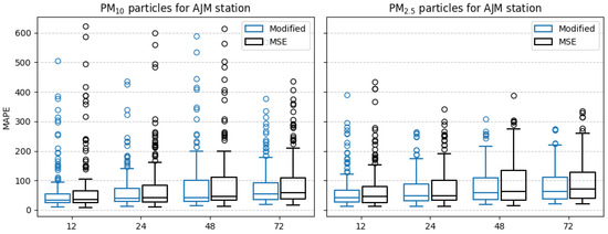
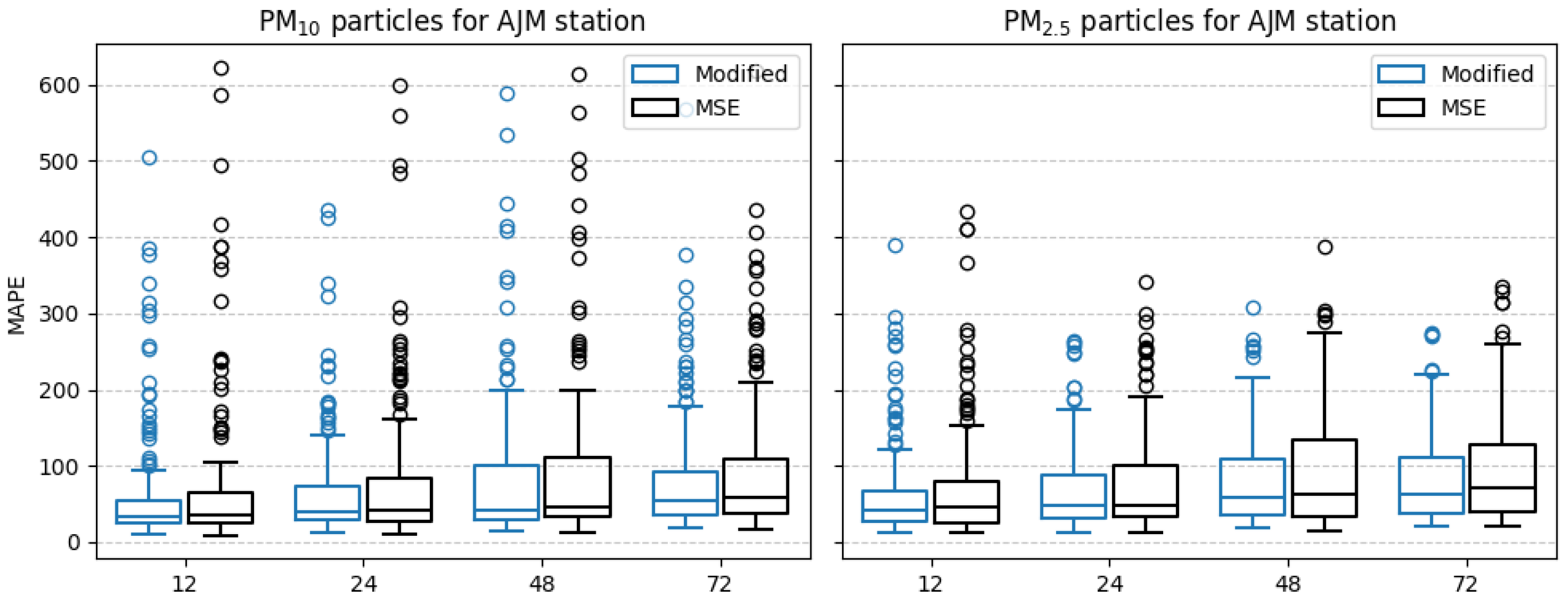
Figure 13. Boxplots of mean absolute percentage error (MAPE) values across different forecast horizons (12, 24, 48 and 72 h) for ${\mathrm{PM}}_{10}$ (left) and ${\mathrm{PM}}_{2.5}$ (right) for AJM station.

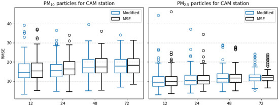
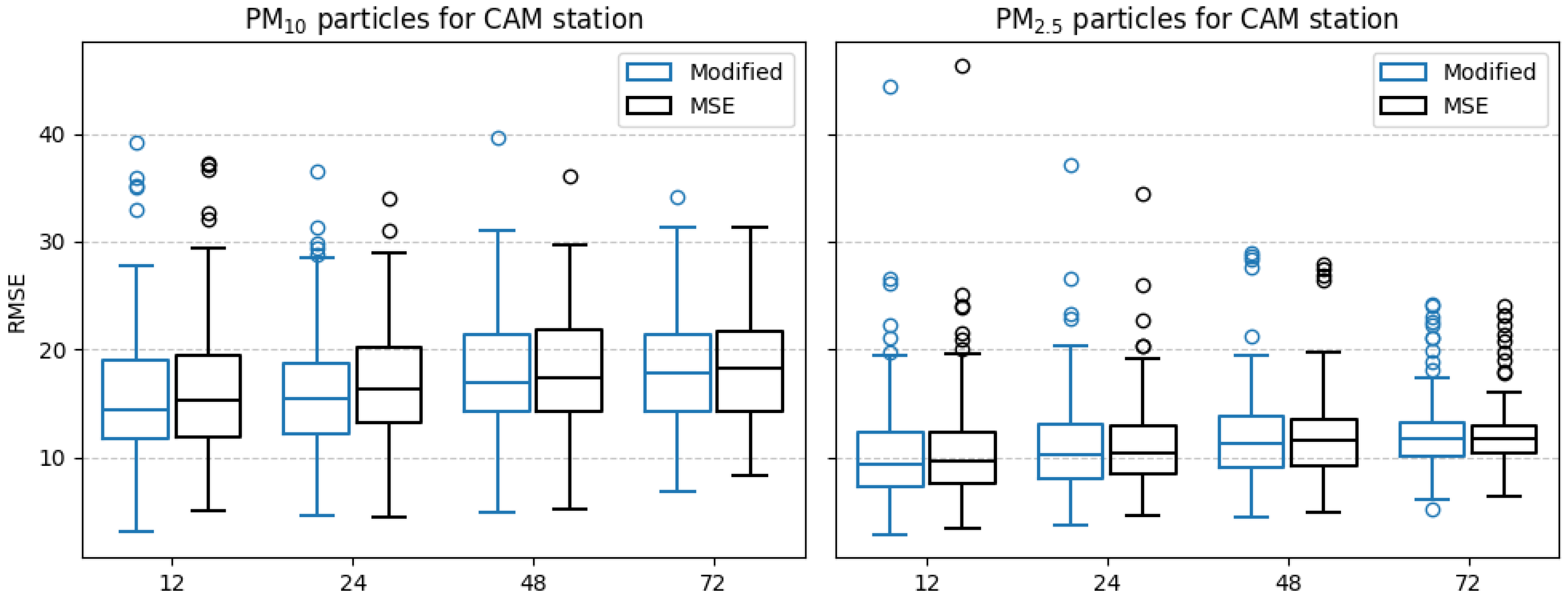
Figure 14. Boxplots of root mean square error (RMSE) values across different forecast horizons (12, 24, 48 and 72 h) for ${\mathrm{PM}}_{10}$ (left) and ${\mathrm{PM}}_{2.5}$ (right) for CAM station.

Figure 15. Boxplots of mean absolute error (MAE) values across different forecast horizons (12, 24, 48 and 72 h) for ${\mathrm{PM}}_{10}$ (left) and ${\mathrm{PM}}_{2.5}$ (right) for CAM station.

Figure 16. Boxplots of mean absolute percentage error (MAPE) values across different forecast horizons (12, 24, 48 and 72 h) for ${\mathrm{PM}}_{10}$ (left) and ${\mathrm{PM}}_{2.5}$ (right) for CAM station.

Figure 17. Boxplots of root mean square error (RMSE) values across different forecast horizons (12, 24, 48 and 72 h) for ${\mathrm{PM}}_{10}$ (left) and ${\mathrm{PM}}_{2.5}$ (right) for MER station.

Figure 18. Boxplots of mean absolute error (MAE) values across different forecast horizons (12, 24, 48 and 72 h) for ${\mathrm{PM}}_{10}$ (left) and ${\mathrm{PM}}_{2.5}$ (right) for MER station.

Figure 19. Boxplots of mean absolute percentage error (MAPE) values across different forecast horizons (12, 24, 48 and 72 h) for ${\mathrm{PM}}_{10}$ (left) and ${\mathrm{PM}}_{2.5}$ (right) for MER station.

Figure 20. Boxplots of root mean square error (RMSE) values across forecast horizons (12, 24, 48, and 72 h) for ${\mathrm{PM}}_{10}$ (left) and ${\mathrm{PM}}_{2.5}$ (right) at the PED station.

Figure 21. Boxplots of mean absolute error (MAE) values across different forecast horizons (12, 24, 48 and 72 h) for ${\mathrm{PM}}_{10}$ (left) and ${\mathrm{PM}}_{2.5}$ (right) for PED station.

Figure 22. Boxplots of mean absolute percentage error (MAPE) values across different forecast horizons (12, 24, 48 and 72 h) for ${\mathrm{PM}}_{10}$ (left) and ${\mathrm{PM}}_{2.5}$ (right) for PED station.

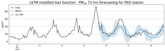
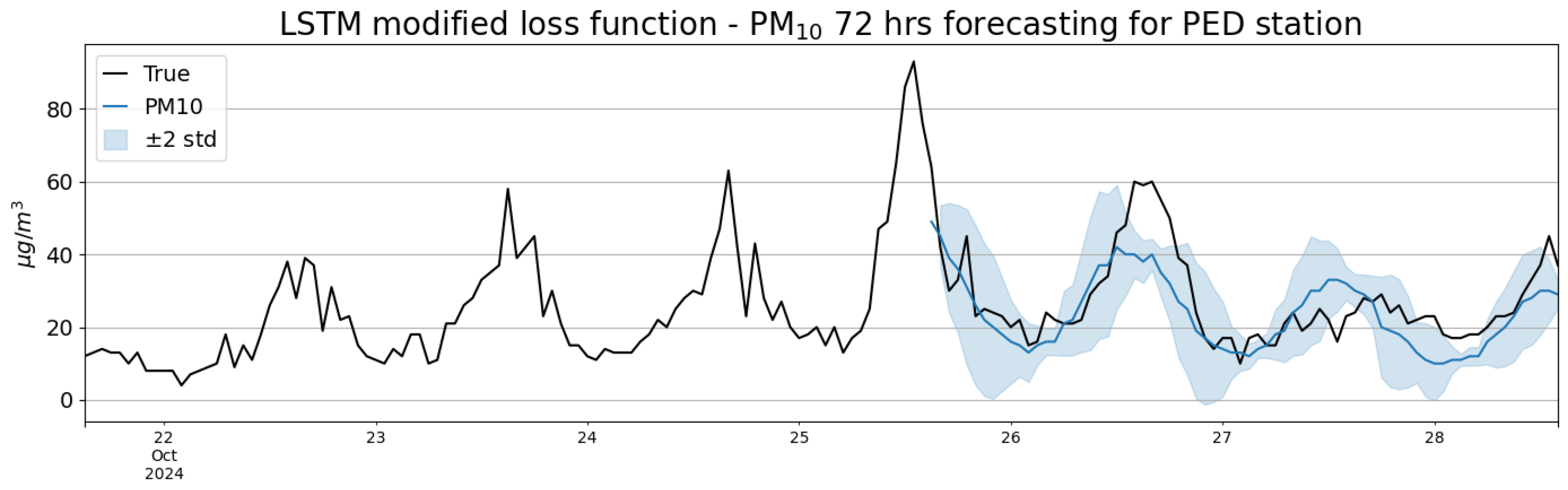
As observed in the results, the LSTM model with the modified loss function shows an improvement in most cases by showing a lower RMSE, MAE and MAPE values for the different forecasting horizons across all stations. Figure 23 shows the LSTM model with a modified loss function for a 72 h forecasting of ${\mathrm{PM}}_{10}$ particles at the PED station.

Figure 23. 72 h forecasting for PED station using LSTM model with modified loss function.

The data presented in the preceding tables and figures demonstrate the effectiveness of the forecasting models. Nonetheless, it is important to note that these models generally exhibit superior performance for ${\mathrm{PM}}_{10}$, compared to ${\mathrm{PM}}_{2.5}$. Additionally, the standard LSTM model surpasses the proposed new model only in a limited number of instances.

4. Discussion

The results obtained demonstrated that the proposed LSTM model with a modified loss function based on Gaussian copulas outperforms the traditional LSTM in forecasting ${\mathrm{PM}}_{10}$ and ${\mathrm{PM}}_{2.5}$ concentrations across the four monitoring sites and at different prediction horizons. The consistent reduction in RMSE, MAE, and MAPE confirms that the incorporation of a statistical method allows the model to capture more dependence between variables.

An important finding is that the proposed model performed particularly well for the prediction of ${\mathrm{PM}}_{10}$ particles at AJM station for the 24-h horizon forecasting, with an RMSE of 10.786 ($\mathsf{\mu }$g/m³), MAE of 8.828 ($\mathsf{\mu }$g/m³) and MAPE of 68.33% (Table 9, Table 10 and Table 11) where the improvements were most significant compared to the baseline model with an RMSE of 11.134 ($\mathsf{\mu }$g/m³), MAE of 9.220 ($\mathsf{\mu }$g/m³) and MAPE of 81.81% (Table 15, Table 16 and Table 17). While for ${\mathrm{PM}}_{2.5}$ particles, again the AJM station for an horizon of 72-h obtained an improvement with an RMSE of 9.082 ($\mathsf{\mu }$g/m³), MAE of 7.065 ($\mathsf{\mu }$g/m³) and MAPE of 81.35% (Table 12, Table 13 and Table 14). In this case, the improvements proved most evident compared to the baseline model with an RMSE of 9.095 ($\mathsf{\mu }$g/m³), MAE of 7.271 ($\mathsf{\mu }$g/m³) and MAPE of 96.74% (Table 15, Table 16 and Table 17).

The results (Figure 11, Figure 12, Figure 13, Figure 14, Figure 15, Figure 16, Figure 17, Figure 18, Figure 19, Figure 20, Figure 21 and Figure 22) also reveal that the improvements are more substantial for ${\mathrm{PM}}_{10}$ than for ${\mathrm{PM}}_{2.5}$. This is likely due to the more stable behavior of ${\mathrm{PM}}_{10}$ concentrations relative to ${\mathrm{PM}}_{2.5}$, suggesting that the addition of more variables, such as wind speed, humidity, and temperature, could help improve performance.

To ensure that the performance of the proposed model was not due to overfitting, several measures were implemented, such as temporal cross-validation, splitting of data into training and test sets in multiple time windows, and moderate hyperparameter tuning shown in Table 3.

Another key advantage of this approach lies in its computational efficiency. The Gaussian copula component integrated into the loss function entails only minimal additional computation, rendering the method lightweight and straightforward to implement. Consequently, a modest modification to a conventional LSTM architecture yields substantial enhancements in predictive performance without appreciably increasing training duration or necessitating advanced hardware.

Although prediction errors predictably escalated at extended forecast horizons (48 and 72 h), the proposed model consistently surpassed the baseline, demonstrating its robustness and stability. Overall, these results underscore the practical value of hybridizing recurrent neural networks with statistical techniques to advance air quality forecasting research.

5. Conclusions

This study presented a model for forecasting ${\mathrm{PM}}_{10}$ and ${\mathrm{PM}}_{2.5}$ concentrations that integrates an LSTM network with a modified loss function that incorporates the Gaussian copula density. The results of four monitoring stations in Mexico City demonstrate that the proposed model consistently outperforms the traditional LSTM across multiple prediction horizons, achieving lower RMSE, MAE, and MAPE values.

The inclusion of the Gaussian copula in the loss function proved effective as a form of statistical regularization, capturing dependencies between variables and mitigating overfitting, thereby enabling better generalization. The validation strategy, based on temporal cross-validation and careful data splitting, ensured that the improvements were not the result of biased training.

The model showed the greatest improvements in the forecasting of particles ${\mathrm{PM}}_{10}$, particularly at the AJM station for the 24 h horizon, while the forecast for particles ${\mathrm{PM}}_{2.5}$ presented smaller but consistent gains, suggesting that the incorporation of meteorological variables could further enhance precision. Despite the expected increase in error with longer horizons, the hybrid approach remained more robust and stable than the baseline model.

An additional advantage of this method is its low computational cost, as the Gaussian copula term requires minimal additional resources. This makes the approach suitable for real-world deployment, because a small modification to the standard LSTM architecture yields an improvement in predictive performance.

In conclusion, the integration of advanced statistical methods with deep learning models represents a real strategy to address complex environmental forecasting tasks for environmental applications. Future work should explore alternative copulas, hybrid architectures, and the inclusion of more meteorological variables to further improve the prediction of ${\mathrm{PM}}_{10}$ and ${\mathrm{PM}}_{2.5}$ particles and enhance real-world applications in air quality management systems.

References

- Fouladi, F.; Bailey, M.J.; Patterson, W.B.; Sioda, M.; Blakley, I.C.; Fodor, A.A.; Jones, R.B.; Chen, Z.; Kim, J.S.; Lurmann, F.; et al. Air pollution exposure is associated with the gut microbiome as revealed by shotgun metagenomic sequencing. Environ. Int. 2020, 138, 105604. [Google Scholar] [CrossRef] [Scilit]
- Calderón-Garcidueñas, L.; Calderón-Garcidueñas, A.; Torres-Jardón, R.; Avila-Ramírez, J.; Kulesza, R.J.; Angiulli, A.D. Air pollution and your brain: What do you need to know right now. Prim. Health Care Res. Dev. 2015, 16, 329–345. [Google Scholar] [CrossRef] [Scilit] [PubMed]
- SEDEMA. Atmospheric Monitoring Directorate. Figshare. Available online: http://www.aire.cdmx.gob.mx/default.php?opc=’ZaBhnmI=’ (accessed on 1 December 2025).
- Montañez, J.A.R.; Fernandez, M.A.A.; Arriaga, S.T.; Arreguin, J.M.R.; Calderon, G.A.S. Evaluation of a Recurrent Neural Network LSTM for the Detection of Exceedances of Particles PM10. In Proceedings of the 2019 16th International Conference on Electrical Engineering, Computing Science and Automatic Control (CCE), Mexico City, Mexico, 11–13 September 2019. [Google Scholar]
- Becerra-Rico, J.; Aceves-Fernández, M.A.; Esquivel-Escalante, K.; Pedraza-Ortega, J.C. Airborne particle pollution predictive model using gated recurrent unit (gru) deep neural networks. Earth Sci. Inform. 2020, 13, 821–834. [Google Scholar] [CrossRef] [Scilit]
- Mauricio-Álvarez, L.E.; Aceves-Fernandez, M.A.; Pedraza-Ortega, J.C.; Ramos-Arreguín, J.M. Evaluation of a transformer-based model for the temporal forecast of coarse particulate matter (PMCO) concentrations. Earth Sci. Inform. 2024, 17, 3095–3110. [Google Scholar] [CrossRef] [Scilit]
- Krogh, A. What are artificial neural networks? Nat. Biotechnol. 2008, 26, 195–197. [Google Scholar] [CrossRef] [Scilit]
- Malevergne, Y.; Sornette, D. Testing the gaussian copula hypothesis for financial assets dependences. Quant. Financ. 2003, 3, 231–250. [Google Scholar] [CrossRef] [Scilit]
- Tootoonchi, F.; Sadegh, M.; Haerter, J.O.; Räty, O.; Grabs, T.; Teutschbein, C. Copulas for hydroclimatic analysis: A practice-oriented overview. Wiley Interdiscip. Rev. Water 2022, 9, 1579. [Google Scholar] [CrossRef] [Scilit]
- Mukhopadhyay, S.; Parzen, E. Nonparametric universal copula modeling. Appl. Stoch. Models Bus. Ind. 2020, 36, 77–94. [Google Scholar] [CrossRef] [Scilit]
- Kolev, N.; Anjos, U.D.; Mendes, B.V. Copulas: A review and recent developments. Stoch. Models 2006, 22, 617–660. [Google Scholar] [CrossRef] [Scilit]
- Manisalidis, I.; Stavropoulou, E.; Stavropoulos, A.; Bezirtzoglou, E. Environmental and health impacts of air pollution: A review. Front. Public Health 2020, 8, 2296–2565. [Google Scholar] [CrossRef] [Scilit] [PubMed]
- Turner, M.C.; Andersen, Z.J.; Baccarelli, A.; Diver, W.R.; Gapstur, S.M.; Pope, C.A., III; Prada, D.; Samet, J.; Thurston, G.; Cohen, A. Outdoor air pollution and cancer: An overview of the current evidence and public health recommendations. CA Cancer J. Clin. 2020, 70, 460–479. [Google Scholar] [CrossRef] [Scilit]
- Hormati, M.; Mohammadi, M.J.; Iswanto, A.H.; Mansourimoghadam, S.; Taifi, A.; Maleki, H.; Mustafa, Y.F.; Dehaghi, B.F.; Afra, A.; Taherian, M.; et al. Consequences and health effects of toxic air pollutants emission by industries. J. Air Pollut. Health 2022, 7, 95–108. [Google Scholar] [CrossRef] [Scilit]
- Arias-Pérez, R.D.; Taborda, N.A.; Gómez, D.M.; Narvaez, J.F.; Porras, J.; Hernandez, J.C. Inflammatory effects of particulate matter air pollution. Environ. Sci. Pollut. Res. 2020, 27, 42390–42404. [Google Scholar] [CrossRef] [Scilit]
- Kampa, M.; Castanas, E. Human health effects of air pollution. Environ. Pollut. 2008, 151, 362–367. [Google Scholar] [CrossRef] [Scilit]
- Bakolis, I.; Hammoud, R.; Stewart, R.; Beevers, S.; Dajnak, D.; MacCrimmon, S.; Broadbent, M.; Pritchard, M.; Shiode, N.; Fecht, D.; et al. Mental health consequences of urban air pollution: Prospective population-based longitudinal survey. Soc. Psychiatry Psychiatr. Epidemiol. 2021, 56, 1587–1599. [Google Scholar] [CrossRef] [Scilit]
- Kutralam-Muniasamy, G.; Pérez-Guevara, F.; Martínez, I.E.; Chari, S.V. Particulate matter concentrations and their association with covid-19-related mortality in mexico during june 2020 saharan dust event. Environ. Sci. Pollut. Res. 2021, 28, 49989–50000. [Google Scholar] [CrossRef] [Scilit] [PubMed]
- Hernández-Escamilla, J.A.; Flores-Margez, J.P.; Shukla, M.K. Particulate matter: Capture and quantification in natural and anthropogenic sources. J. Environ. Anal. Toxicol. 2015, 5, 2161-0525. [Google Scholar] [CrossRef]
- Mainka, A.; Żak, M. Synergistic or antagonistic health effects of long- and short-term exposure to ambient NO2 and PM2.5: A review. Int. J. Environ. Res. Public Health 2022, 19, 14079. [Google Scholar] [CrossRef] [Scilit] [PubMed]
- Kyung, S.Y.; Jeong, S.H. Particulate-matter related respiratory diseases. Tuberc. Respir. Dis. 2020, 83, 116–121. [Google Scholar] [CrossRef] [Scilit] [PubMed]
- Ramírez-Sánchez, H.U.; Fajardo-Montiel, A.L. Air pollution in medium-sized mexican cities. Asian J. Environ. Ecol. 2023, 22, 1–15. [Google Scholar] [CrossRef] [Scilit]
- Hollenbach, F.M.; Bojinov, I.; Minhas, S.; Metternich, N.W.; Ward, M.D.; Volfovsky, A. Multiple imputation using gaussian copulas. Sociol. Methods Res. 2018, 50, 1259–1283. [Google Scholar] [CrossRef] [Scilit]
- Moghar, A.; Hamiche, M. Stock market prediction using lstm recurrent neural network. Procedia Comput. Sci. 2020, 170, 1168–1173. [Google Scholar] [CrossRef] [Scilit]
- Uzair, M.; Jamil, N. Effects of Hidden Layers on the Efficiency of Neural networks. In Proceedings of the 2020 IEEE 23rd International Multitopic Conference (INMIC), Bahawalpur, Pakistan, 5–7 November 2020. [Google Scholar]
- Gonzalez, J.; Yu, W. Non-linear system modeling using lstm neural networks. IFAC-PapersOnLine 2018, 51, 485–489. [Google Scholar] [CrossRef] [Scilit]
- Hua, Y.; Zhao, Z.; Li, R.; Chen, X.; Liu, Z.; Zhang, H. Deep learning with long short-term memory for time series prediction. IEEE Commun. Mag. 2019, 57, 114–119. [Google Scholar] [CrossRef] [Scilit]
- Li, Z.; Yim, S.H.; Ho, K.F. High temporal resolution prediction of street-level PM2.5 and nox concentrations using machine learning approach. J. Clean. Prod. 2020, 268, 121975. [Google Scholar] [CrossRef] [Scilit]
- Randall, T.; Koo, J.; Videau, B.; Kruse, M.; Wu, X.; Hovland, P.; Hall, M.; Ge, R.; Balaprakash, P. Transfer-learning-based Autotuning using Gaussian Copula. In Proceedings of the 37th International Conference on Supercomputing, Orlando, FL, USA, 21–23 June 2023. [Google Scholar]
- Razali, H.M.; Wah, Y.B. Power comparisons of shapiro-wilk, kolmogorov-smirnov, lilliefors and anderson-darling tests. J. Stat. Model. Anal. 2011, 2, 21–33. [Google Scholar]
- Scholz, F.W.; Stephens, M.A. K-sample anderson–darling tests. J. Am. Stat. Assoc. 1987, 82, 918–924. [Google Scholar] [CrossRef] [Scilit]
- Asar, O.; Ilk, O.; Dag, O. Estimating box-cox power transformation parameter via goodness-of-fit tests. Commun. Stat. Simul. Comput. 2014, 49, 91–105. [Google Scholar] [CrossRef] [Scilit]
Disclaimer/Publisher’s Note: The statements, opinions and data contained in all publications are solely those of the individual author(s) and contributor(s) and not of MDPI and/or the editor(s). MDPI and/or the editor(s) disclaim responsibility for any injury to people or property resulting from any ideas, methods, instructions or products referred to in the content. |
© 2026 by the authors. Licensee MDPI, Basel, Switzerland. This article is an open access article distributed under the terms and conditions of the Creative Commons Attribution (CC BY) license.