Multi-Step Forecasting of Weekly Dengue Cases Using Data Augmentation and Convolutional Recurrent Neural Networks

Abstract

Dengue case forecasting is important for the prevention and early control of outbreaks, as well as for the optimization of healthcare resources, among other aspects. This study addresses the need to develop increasingly accurate forecasting models that can support informed decision-making before and during dengue epidemics. Accordingly, two new models based on convolutional and recurrent neural networks, namely ConvLSTM and ConvBiLSTM, combined with data augmentation based on linear interpolation, are proposed. As a case study, weekly dengue cases in Peru from 2000 to 2024 are used. The proposed models are compared with well-known recurrent neural network-based models such as LSTM, BiLSTM, GRU, and BiGRU, both with and without data augmentation. The results show that the proposed models with data augmentation achieve comparable and superior performance to the benchmark models, while also exhibiting a lower average computational cost.

1. Introduction

Dengue is a major public health concern [1] in tropical and subtropical regions [2], with recurrent outbreaks posing significant challenges to healthcare systems worldwide. Its rapid spread, driven by factors such as climate variability and urbanization [3], has led to a substantial increase in reported cases in recent decades, particularly in Latin America, Southeast Asia, and Africa.

In Peru, dengue outbreaks have shown pronounced temporal variability. In 2024, a total of 280,242 cases were reported, whereas in 2025 only 39,211 cases were registered, representing a sharp decrease compared to the previous year. Despite this variability, Peru continues to exhibit one of the highest dengue-related mortality rates in Latin America, underscoring the need for effective tools to support early outbreak detection and public health decision-making.

Dengue transmission is strongly influenced by climatic conditions [4] such as temperature, rainfall, and humidity, which favor the proliferation of the Aedes aegypti mosquito [5]. Accurate forecasting of dengue cases weeks in advance enables health authorities to intensify vector control measures, implement preventive campaigns, and optimize healthcare resource allocation, thereby reducing the risk of small outbreaks escalating into large-scale epidemics.

In this context, forecasting dengue cases has emerged as a critical component of early warning systems [6]. Recent studies have increasingly relied on data-driven and deep learning-based approaches to capture the complex temporal dynamics of dengue transmission. Motivated by this need, this study proposes a novel dengue case forecasting framework that integrates data augmentation strategies with spatiotemporal neural network architectures, specifically ConvLSTM [7] and ConvBiLSTM [8] models, to improve predictive performance under limited and highly variable data scenarios.

Based on the literature review, it is observed that most studies on dengue case forecasting primarily focus on multivariate models based on deep learning techniques, particularly LSTM [9] and its variants. However, univariate models have been scarcely explored, despite requiring fewer data and being potentially more suitable in scenarios where the availability of explanatory variables is limited. This is particularly critical given that dengue time series are often short, highly variable, and characterized by extreme outbreak peaks, which pose significant challenges for data-hungry deep learning models [10]. Furthermore, both single-step and multi-step forecasting frameworks in existing studies rarely conduct a systematic analysis of data augmentation techniques as a strategy to enhance model performance. This lack of investigation limits the understanding of the impact of data augmentation on dengue outbreak prediction, especially in contexts characterized by short or highly variable time series.

The main inspiration for developing the proposal comes from works such as [11] and [12], where for multi-step predictions the historical univariate data were organized in a matrix (2D) format, achieving superior results compared to models that operate only with data arranged in a vector (1D) format.

A univariate model that processes input data arranged in a two-dimensional (2D) format is capable of capturing not only temporal dependencies but also spatial correlations induced by the inherent width–height structure of the data representation. In contrast, conventional LSTM models that operate on one-dimensional (1D) input sequences assume the presence of temporal correlations only. A key limitation of the former approach lies in the transformation of a 1D vector into a 2D representation: depending on the selected number of rows, the effective number of training samples is reduced, as the data are partitioned into matrix rows rather than individual observations. This reduction in sample size may increase the risk of overfitting; therefore, the incorporation of data augmentation techniques becomes crucial to enhance generalization performance.

The proposed approach is compared with various deep learning models including Long Short-Term Memory (LSTM) [13], Bidirectional LSTM (BiLSTM) [14], Gated Recurrent Unit (GRU) [15], and Bidirectional GRU (BiGRU) [16], with prediction steps including 2, 4, and 6 weeks.

The forecasting horizons of 2, 4, and 6 weeks were selected to reflect short-, medium-, and long-term decision-making needs in dengue surveillance. Short-term forecasts support early warning detection, while medium- and long-term horizons are critical for vector control planning and healthcare resource allocation.

The main contributions of this work are listed below:

-

A new approach for multi-step dengue cases forecasting based on convolutional neural networks and recurrent neural networks.

-

A data augmentation technique for time series regression based on linear interpolation.

-

A comparative study between the proposed approach and different benchmark models.

This study hypothesizes that incorporating data augmentation techniques can enhance the predictive performance of CNN + RNN-based models in dengue forecasting, particularly in scenarios characterized by short and highly variable time series.

The remainder of the paper is structured as follows: Section 2, which describes previous research on the topic. Section 3, which details the study’s methodology, including the description of the proposed approach. Section 4, where the achieved results and their implications are analyzed. Finally, Section 5 summarizes the main findings of this study.

2. Literature Review

2.1. Data Augmentation Related Works

Several data augmentation techniques have been developed for time series, grounded on three main pillars [17]: traditional algorithms, variational autoencoders (VAE), and generative adversarial network (GAN). In this work, we focus on the former, since the proposed approach implements one based on traditional algorithms such as linear interpolation.

Traditional algorithms are defined as techniques that take samples from the input data and generate new ones through various transformations such as time warping [18], jittering [19,20], window slicing [21], window warping [22], time flipping [23], and others.

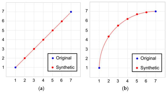
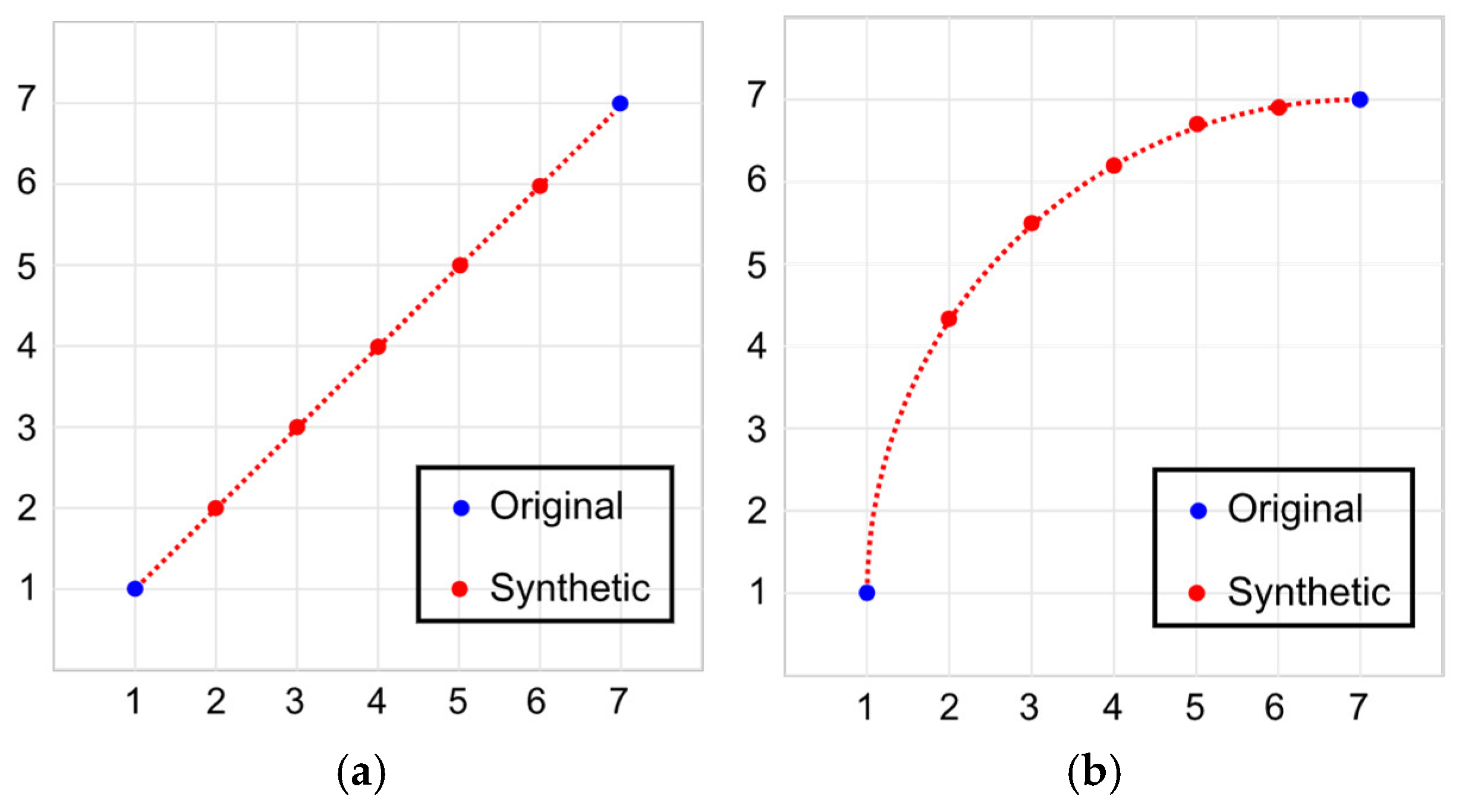
Time warping is one of the most popular techniques and can be implemented in various ways, such as linear interpolation [24,25] or polynomial interpolation [26,27]. Time warping consists of adding synthetic values between each pair of values in the time series without altering its 1D nature. Figure 1 shows how time warping is used in time series.

Figure 1. Data augmentation with time warping. (a) Linear interpolation and (b) polynomial interpolation.

2.2. One-Step Dengue Related Works

According to the literature review, only five studies were found on one-step forecasting of dengue cases. In [28], the authors propose an LSTM model to predict weekly dengue cases in Puerto Rico, achieving an RMSE of 15.67 cases. Then, in [29], an LSTM model is also proposed to predict monthly dengue cases in the Philippines, achieving an RMSE of 73.17 cases. In [30], the authors proposed an LSTM with an attention layer to predict weekly dengue cases in Malaysia, achieving an RMSE of 3.10 cases. Table 1 summarizes the works on one-step forecasting for dengue cases. In [4], a multivariate CNN-LSTM-based model was used to predict weekly dengue cases in Brazil, achieving an RMSE of 10.52. In [31], the authors implemented a multivariate model to predict weekly dengue cases in Singapore, using decomposition techniques and AutoML, achieving a MAPE of 14.27%. In [32], the authors implement an ARIMA model to predict monthly dengue cases, achieving a MAPE of 43.40%. In [33], the authors implement several machine learning models, such as XGBoost, SVR, and MLP, with XGBoost being the most accurate, achieving a MAPE of 0.129%. In [34], the author implements several multivariate machine learning models, with Random Forest emerging as the best-performing model, achieving a MAPE of 4.2%.

Table 1. One-step related works for dengue forecasting.

Work	Country	Technique	Freq.	Step Size	Metric	Value
[28]	Puerto Rico	LSTM	Weekly	1	RMSE	15.67
[29]	Philippines	LSTM	Monthly	1	RMSE	73.17
[30]	Malaysia	LSTM-ATT	Weekly	1	RMSE	3.10
[35]	Brazil	CatBoost-SVM-LSTM	Monthly	1	nRMSE	[0.041–0.274]
[36]	Brazil	LSTM-ARIMA	Monthly	1	MAPE	32.19%
[4]	Brazil	CNN-LSTM	Weekly	1	RMSE	10.52
[31]	Singapore	AutoML	Weekly	1	MAPE	14.27%
[32]	Thailand	ARIMA	Monthly	1	MAPE	43.40%
[33]	Bangladesh	XGBoost	Weekly	1	MAPE	0.129%
[34]	Bangladesh	RF	Daily	1	MAPE	4.2%

2.3. Multi-Step Dengue Related Works

LSTM is one of the most widely used models for multi-step forecasting, and it is implemented in related works such as [37,38,39,40]. Another group of studies uses LSTM variants, such as LSTM with attention layers (LSTM-ATT), as in [41]; others work with bidirectional models like BiLSTM in [29]; and others use GRU models, as in [38]. Only one study, [42], implemented an optimization algorithm known as particle swarm optimization (PSO) combined with a neural network known as generalized regression neural network (GRNN). Another group of works uses machine learning techniques such as support vector machine (SVM) and multi-layer perceptron [43] and random forest [44]. One study [45] was identified that applied a statistical technique, the least absolute shrinkage and selection operator (LASSO), for forecasting weekly dengue cases. Another standalone study [46] implements a Bayesian model. These works are summarized in Table 2.

Table 2. Multi-step related works for dengue forecasting.

Work	Country	Technique	Freq.	Step Size	Metric	Value
[45]	Singapore	LASSO	Weekly	[1,12]	MAPE	[17.00– 24.00]
[37]	China	LSTM	Monthly	[1,12]	RMSE	[54.06–43.10]
[43]	China	SVM, MLP	Weekly	[1,8]	R2	[0.80–0.36]
[44]	Colombia	RF	Weekly	[1,12]	MAE	[13.86–26.76]
[41]	Vietnam	LSTM-ATT	Monthly	[1,3]	RMSE	[0.529–9.544]
[38]	Singapore	RNN, GRU, LSTM, BiLSTM, CNN	Weekly	[1,4]	MAPE	[12.27–17.89]
[42]	Indonesia	EMD-GRNN-PSO		[1,3]	MSE	[0.0001]
[39]	Brazil	LSTM		[4]	MAPE	[21.87–29.95]
[47]	Singapore	BiLSTM	Weekly	[1,4]	MAPE	[12.12–14.62]
[40]	Brazil	LSTM	Weekly	[4,12]	MAPE	[19.63–29.11]
[46]	Singapore	Bayes	Weekly	[2,8]	AUC	[97.8–94.2]

According to the literature review, it is evident that most of the studies were conducted for Asian countries, with only a few focusing on Latin America. Likewise, the majority of the models are multivariable. All the implemented models work with the original 1D form of the time series; none of them organize the time series in a matrix format. In this work, the data is arranged in a matrix (2D) format, leveraging the spatial capabilities of convolutional neural networks such as CNNs, and the sequential capabilities of recurrent neural networks such as LSTMs.

ConvLSTM and ConvBiLSTM architectures were selected due to their ability to jointly model local temporal patterns through convolutional operations and long-range dependencies via recurrent gating mechanisms. This combination is particularly suitable for highly variable epidemiological time series, where abrupt changes and outbreak peaks must be captured at multiple temporal scales.

While alternative architectures such as temporal convolutional networks (TCNs) and transformer-based forecasters have demonstrated strong performance in large-scale multivariate forecasting tasks, they typically require extensive hyperparameter tuning and larger datasets to fully exploit their attention mechanisms. In contrast, ConvLSTM-based models offer a more stable and data-efficient learning process, which is advantageous in univariate dengue forecasting scenarios characterized by limited explanatory variables and moderate dataset sizes.

Furthermore, the bidirectional variant (ConvBiLSTM) enables the model to learn richer temporal representations within the input window, improving robustness to local fluctuations without introducing the computational overhead associated with transformer-based models.

The objective of this study is not to exhaustively benchmark all state-of-the-art architectures, but to analyze the impact of data augmentation on convolutional–recurrent models under controlled experimental conditions.

The main differences between the studies in the literature and the proposed approach are summarized in Table 3.

Table 3. Main differences between this study and related works.

Related Works	This Study
- Most studies were conducted using dengue data from Asian countries, with only five focusing on Latin America (Colombia, Puerto Rico, and Brazil).	- The study used weekly dengue case data from Peru.
- The majority of the works exploit only the original 1D form of time series, mainly using models such as LSTM and its variants.	- The 1D time series is converted into a 2D format, and the spatiotemporal characteristics of the series are leveraged using a hybrid ConvLSTM and ConvBiLSTM model.
- None of the studies applied data augmentation to enhance the forecasting performance of the models.	- A data augmentation strategy was implemented to reduce prediction errors.
- Most of them implemented multivariate models.	- The proposed method is univariate; it works only with historical data.

3. Materials and Methods

3.1. Data Collection

The data related to weekly dengue cases in Peru, used in this study, were downloaded from the repository of the Ministry of Health of Peru from the following link: https://www.dge.gob.pe/sala-situacional-dengue/ accessed on 1 July 2024.

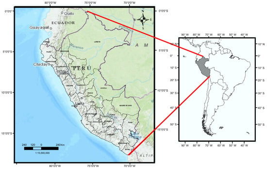
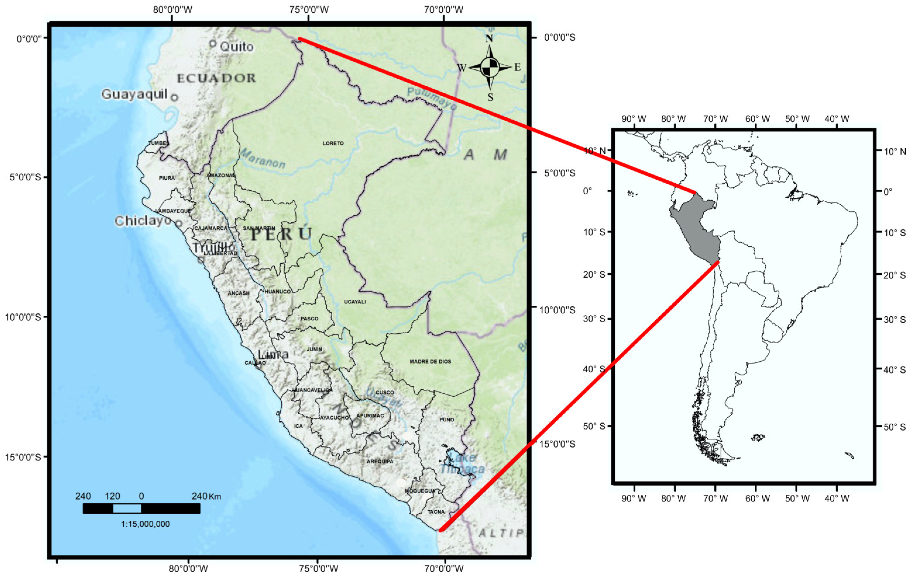
The dataset contains weekly dengue case data from the years 2000 to 2024. Figure 2 shows the location of Peru in South America.

Figure 2. Location of Peru in South America.

3.2. Data Preparation

The dataset contains a total of 1321 records, corresponding to Peruvian weekly dengue cases.

3.2.1. Matrix Organization

In this study, the proposed approach for multi-step forecasting predicts 2, 4, and 6 weeks. Unlike most state-of-the-art models for dengue forecasting, the historical data is structured in a matrix format.

To predict 2 weeks, the data is organized into a n × 2 matrix, where (n) is the number of rows in the matrix, and 2 represents the number of weeks. Similarly, to predict 4 weeks, the data is organized into a n × 4 matrix. To predict 6 weeks, the data is organized into a n × 6 matrix.

It is important to highlight that the number of columns in the matrix will depend on the number of prediction steps of the model. For example, if we want to predict one step ahead, the number of columns will be 1; if we want to predict two steps ahead, the number of columns will be 2; and so on.

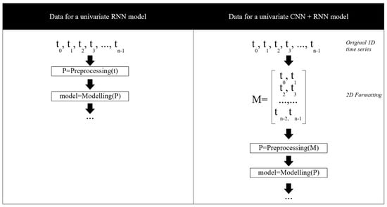
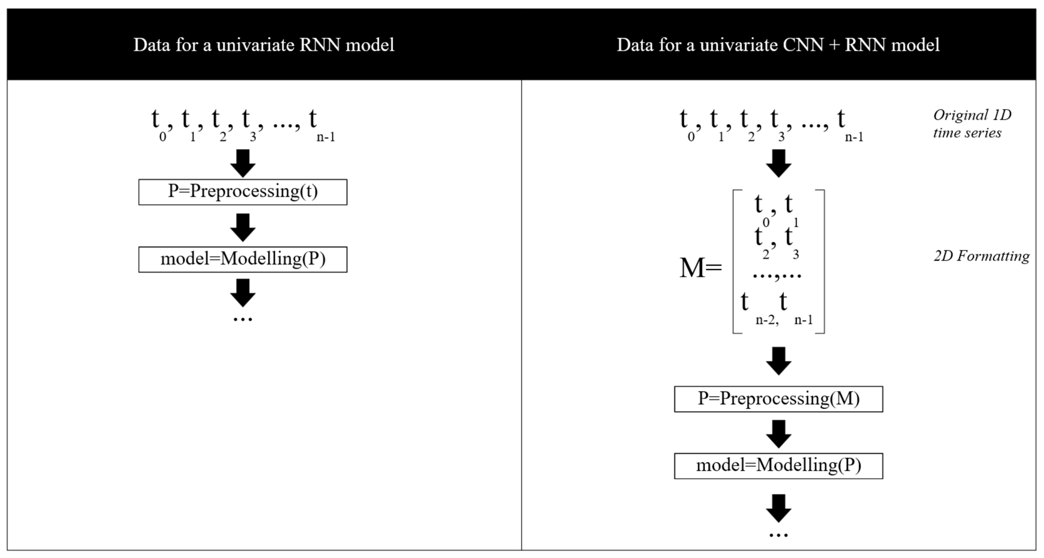
Figure 3 illustrates the differences in the preprocessing steps between a standard RNN and the matrix organization for the proposed CNN + RNN-based models.

Figure 3. Illustration of how the original time series is used in an RNN and in a CNN + RNN architecture. The left panel shows the processing of the time series t for the univariate RNN used in this study, while the right panel presents the processing of the time series t for the univariate CNN + RNN-based models.

The matrix organization of the time series allows the CNN component to capture local temporal patterns across multiple consecutive time steps within each window. By reshaping the 1D time series into a 2D representation, convolutional filters can learn short-term dependencies and local structures that are not explicitly modeled when using a standard univariate RNN alone.

3.2.2. Data Splitting

The dataset was partitioned into training, validation, and test sets using a 70/15/15 split, strictly following the chronological order of the time series. The earliest 70% of the observations were used for training, the subsequent 15% for validation, and the most recent 15% for testing, thereby preventing any form of data leakage.

3.2.3. Data Augmentation

Once the data was organized in matrix form, the next step is to perform the corresponding data augmentation in order to avoid model overfitting. For this purpose, linear interpolation was used. Data augmentation through interpolation was applied exclusively to the training set and only after the chronological data split. The validation and test sets remained unchanged to prevent any leakage of future information into the training process.

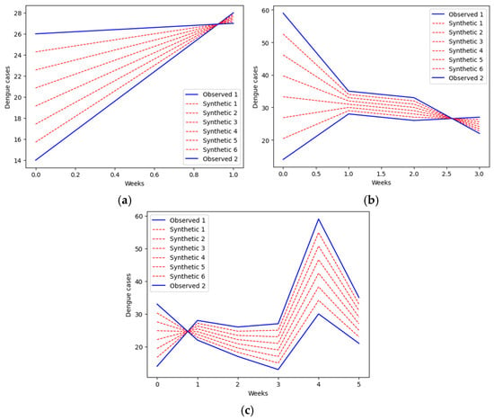
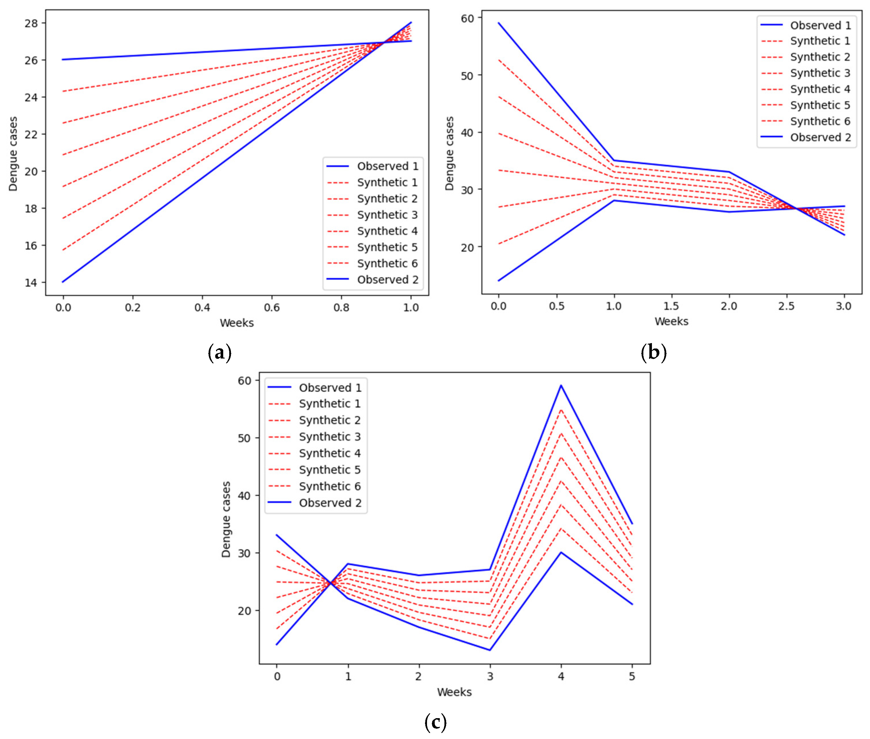
Examples of the result of this process are shown in Figure 4.

Figure 4. Six synthetic rows obtained through linear interpolation from two rows of observed cases. (a) The Observed1 data correspond to the first two weeks of the year 2000, and the Observed2 data correspond to the next two weeks of the same year. (b) The Observed1 data correspond to the first month of the year 2000, and Observed2 correspond to the next month of the same year. (c) The Observed1 data correspond to the first six weeks of the year 2000, and the second row corresponds to the following six weeks of the same year.

3.2.4. Normalization

To implement neural networks and ensure fast convergence, it is necessary to normalize the time series. In this study, min–max normalization [48] was used, computed as shown in Equation (1).

$$x^{\prime }={\displaystyle \frac{(x-\min \left(x\right))}{\max \left(x\right)-\mathrm{m}\mathrm{i}\mathrm{n}\left(x\right)}}$$

(1)

where x′ is the normalized value, x is the value to be normalized, and min(x) and max(x) are the minimum and maximum values of the vector to be normalized.

Min–max normalization was applied using scaling parameters (minimum and maximum values) computed exclusively from the training set. These parameters were then fixed and applied to the validation and test sets to prevent information leakage.

3.3. Modelling

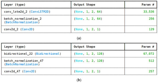
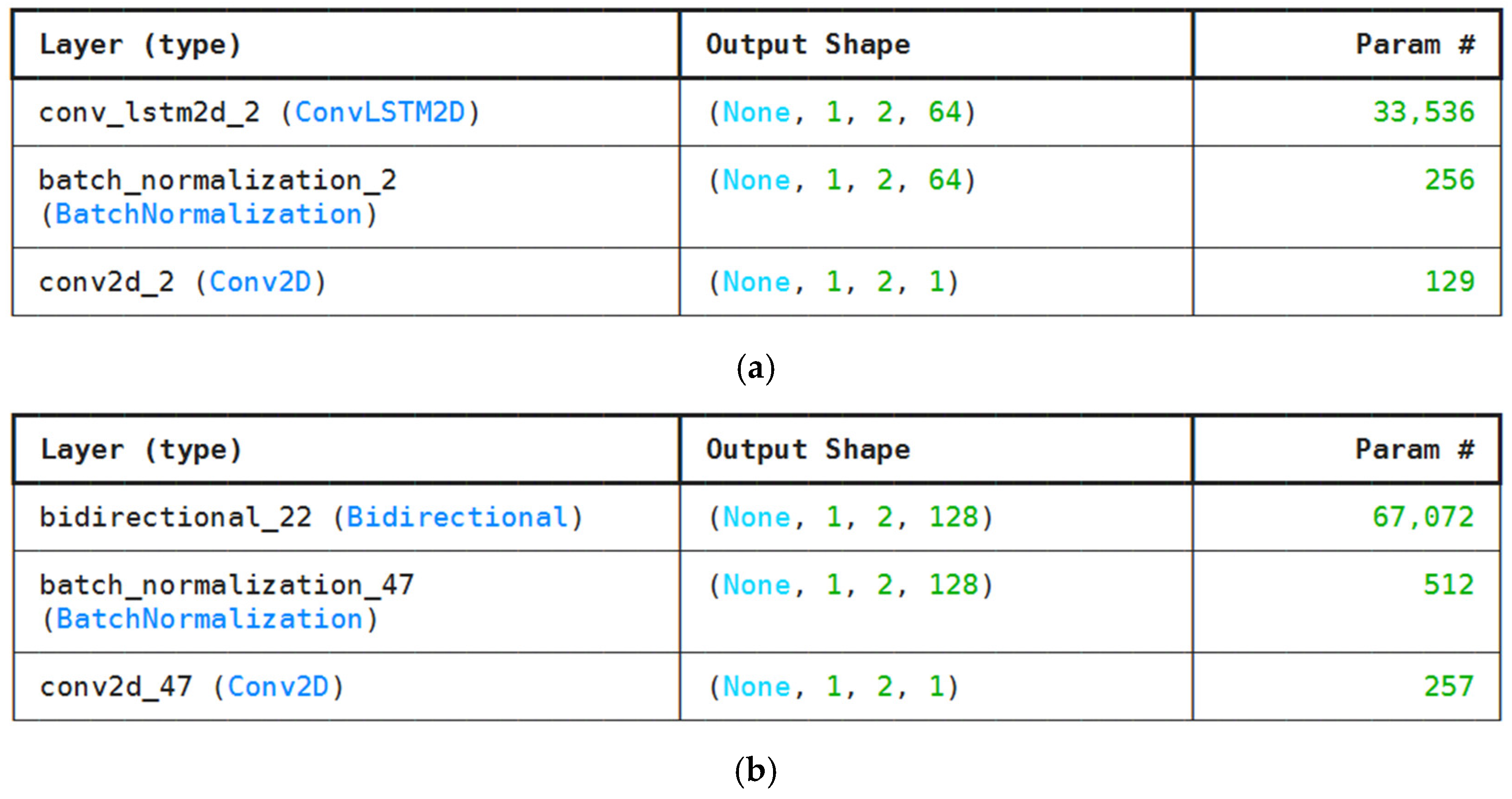
The model architectures in the proposed approach are shown in Figure 5.

Figure 5. Architecture of models. (a) ConvLSTM and (b) ConvBiLSTM.

The first of the implemented models of the proposed approach is based on a ConvLSTM2D architecture, which is designed to simultaneously capture temporal and spatial dependencies in matrix-structured data. The model input corresponds to a sequence of previously normalized matrices. The model is composed of the following layers.

The ConvLSTM2D layer, which contains 64 filters, with a (1,2) kernel, padding same, ReLU as the activation function, and does not return sequences. As shown in Figure 5a, a (1,2) kernel is applied to a matrix with n rows and 2 columns. Similarly, a (1,4) kernel is required for a matrix with 4 columns, while a (1,6) kernel is required for a matrix with 6 columns. In summary, a ConvLSTM2D layer is an extension of the classical LSTM in which linear (matrix-based) operations are replaced by convolutions. The gating mechanisms remain the same as in a standard LSTM, namely the forget gate, input gate, cell state, and output gate.

The BatchNormalization layer normalizes the activation of the previous output, speeding up training convergence and improving model stability. The Conv2D layer has 1 filter, a (1,2) kernel, padding same, and linear activation for regression tasks. This layer acts as a spatial decoder that transforms the latent representations into the final predicted matrix output.

The Conv2D layer serves as the output layer of the ConvLSTM model for regression, performing the final convolutional projection and predicting a single row with 2, 4, or 6 columns corresponding to the prediction horizons analyzed in this study.

The second model is similar to the previous one; however, the main difference is the use of a bidirectional first layer (ConvBiLSTM2D) instead of ConvLSTM2D, which enables the input matrix to be processed in both forward and backward temporal directions. Both architectures can be observed in Figure 5.

To ensure a controlled and reproducible comparison, the main architectural hyperparameters (e.g., number of layers and hidden units) were kept consistent across all models. This design choice allows isolating the impact of the proposed data augmentation strategy and recurrent architecture, rather than performance differences arising from extensive hyperparameter tuning. While this strategy may not yield the optimal configuration for each individual architecture, it provides a fair baseline for comparative evaluation under equivalent model capacity.

All the implemented models used the same number of layers and neurons in each layer. They were implemented in the Jupyter IDE using the TensorFlow 2.18.0 library in Python language 3.11.7. The lookback for each model is twelve weeks. The models were compiled with ‘mse’ as the loss function and ‘adam’ as the optimizer, with a batch size of 16 and 50 training epochs.

All models were trained using the same training protocol to ensure a controlled and fair comparison across architectures and data augmentation configurations. A fixed number of training epochs and a constant learning rate were used for all experiments, and model selection was based on validation performance.

Although standard robustness techniques such as early stopping, learning-rate scheduling, and repeated trials with multiple random seeds can further improve training stability, they were not incorporated in this study in order to maintain experimental consistency and computational feasibility across all evaluated models.

Despite this, the proposed models exhibit consistent performance improvements across multiple forecasting horizons, suggesting that the observed gains are not driven by isolated training instabilities.

3.4. Evaluation

The achieved results are evaluated using three metrics, which include: Root Mean Squared Error (RMSE), which allows assessing the prediction error in terms of the original values of the time series; Mean Absolute Percentage Error (MAPE), which evaluates the results in percentage terms; and finally, the correlation coefficient R, which measures the level of correlation between the observed and predicted data. Equations (2)–(4) enable their implementation.

$$RMSE=\sqrt{{\displaystyle \frac{\sum _{i=1}^n{\left(P_i-X_i\right)}^2}{n}}}$$

(2)

$$MAPE={\displaystyle \frac{1}{n}}{\sum }_{i=1}^n\left|{\displaystyle \frac{\left(X_i-P_i\right)}{X_i}}\ast 100\right|$$

(3)

$$R=\sqrt{{\displaystyle \frac{ \sum _{i=1}^n(P_i-\overline{P})(X_i-\overline{X})}{\sum _{i=1}^n{\left(P_i-\overline{P}\right)}^2\sum _{i=1}^n{\left(X_i-\overline{X}\right)}^2}}}$$

(4)

where $P_i$ is each predicted value, $X_i$ is each observed value, n is the total number of predicted data points, $\overline{P}$ is the mean of the predicted data, and $\overline{X}$ is the mean of the observed data.

RMSE and the correlation coefficient (R) were selected to evaluate overall predictive accuracy and linear association between observed and predicted values. Additionally, MAPE was included due to its widespread use in related dengue forecasting studies and its intuitive percentage-based interpretation.

However, it is important to note that MAPE can be unstable for epidemiological time series when observed values are small, as is often the case during non-outbreak periods. In such situations, small absolute errors may lead to disproportionately large percentage errors, potentially overemphasizing model deficiencies in low-incidence intervals.

This limitation is particularly relevant for dengue case forecasting, which is characterized by high variability and abrupt transitions between low and peak incidence periods. Consequently, MAPE results should be interpreted with caution and considered complementary to RMSE-based evaluations.

MAE was added as an alternate metric in Appendix A.

Model evaluation was conducted using a single, strictly chronological train–validation–test split in order to ensure temporal consistency and avoid information leakage. This evaluation design allows for a controlled comparison of model architectures and data augmentation strategies under identical conditions.

While rolling-origin (walk-forward) evaluation is widely regarded as a best practice in time series forecasting, its application would require multiple retraining cycles and substantially increase computational cost, particularly for deep convolutional–recurrent architectures combined with data augmentation.

Therefore, a fixed split was adopted in this study to balance methodological rigor and experimental feasibility. Future work will extend the evaluation protocol to rolling-origin validation to further assess temporal robustness.

4. Results and Discussions

4.1. Results

This section presents and describes the results achieved by the proposed approach including models ConvLSTM and ConvBiLSTM both without and with data augmentation.

According to Table 4, it can be observed that, in terms of RMSE, for a two-step prediction horizon, the best-performing model is ConvLSTM with four synthetic rows (DA4 + ConvLSTM), which also achieves the best performance for the four- and six-step prediction horizons. In contrast to ConvLSTM, ConvBiLSTM exhibits different optimal models for each prediction horizon. Furthermore, it is observed that, in all cases, the data augmentation technique proposed in this study improves the performance of the baseline models.

Table 4. Results in terms of RMSE of the Proposed Approach.

Model	Prediction Steps
	2	4	6
ConvLSTM	3041.8464	4443.3142	3983.9429
DA2 + ConvLSTM	1583.5745	2105.9220	4458.1269
DA4 + ConvLSTM	300.1274	1092.9905	1473.1886
DA6 + ConvLSTM	1008.8756	1500.7813	1910.4980
ConvBiLSTM	2872.8847	12,540.7191	5177.2140
DA2 + ConvBiLSTM	1547.9647	2409.0993	3176.6682
DA4 + ConvBiLSTM	1861.0425	1481.4508	2068.3653
DA6 + ConvBiLSTM	2138.4653	2753.9465	1512.5834

The large RMSE gap observed in Table 4 between ConvLSTM without data augmentation and DA4 + ConvLSTM for the two-step forecasting horizon is primarily explained by the behavior of RMSE under highly variable epidemiological conditions. Weekly dengue case series are characterized by abrupt outbreak peaks, where a small number of large prediction errors can disproportionately inflate RMSE values.

The baseline ConvLSTM model, trained without data augmentation, exhibits poor generalization during these extreme outbreak periods, resulting in a limited number of very large errors that dominate the RMSE. In contrast, the proposed DA4 strategy increases the effective density of training samples in high-variability regions through interpolation, allowing the model to better learn outbreak dynamics and significantly reduce peak-related errors.

As a result, the reduction in RMSE is not linear but rather driven by the mitigation of a small number of extreme prediction failures. Importantly, all models were trained and evaluated under the same strictly chronological data split and identical evaluation protocol, ruling out information leakage as a cause of the observed performance gap.

According to Table 5, in terms of MAPE, unlike RMSE, it is observed that the best-performing models are not the same for each prediction horizon. Thus, for the two-step prediction horizon, the best model is ConvLSTM with four synthetic rows (DA4 + ConvLSTM), achieving a MAPE of 6.81%. For the four-step prediction horizon, ConvBiLSTM with two synthetic rows (DA2 + ConvBiLSTM) yields the best MAPE (15.31%). Finally, for the six-step prediction horizon, ConvBiLSTM with six synthetic rows (DA6 + ConvBiLSTM) achieves the lowest MAPE (16.08%).

Table 5. Results in terms of MAPE of the Proposed Approach.

Model	Prediction Steps
	2	4	6
ConvLSTM	58.33	59.20	64.70
DA2 + ConvLSTM	20.84	19.35	69.05
DA4 + ConvLSTM	6.81	21.05	34.01
DA6 + ConvLSTM	16.22	21.45	17.29
ConvBiLSTM	44.27	86.78	57.41
DA2 + ConvBiLSTM	27.00	21.97	59.24
DA4 + ConvBiLSTM	23.45	15.31	25.12
DA6 + ConvBiLSTM	27.77	28.48	16.08

The observed discrepancies between RMSE- and MAPE-based rankings highlight the known sensitivity of MAPE to low observed values, reinforcing the importance of multi-metric evaluation in highly variable epidemiological time series.

According to Table 6, in terms of the correlation coefficient (R), similar to RMSE, only one model exhibits the best performance. For the two-, four-, and six-step prediction horizons, ConvLSTM with four synthetic rows achieves the highest correlation values of 0.9982, 0.9749, and 0.9665, respectively. These results confirm the contribution of the proposed data augmentation technique to improving prediction accuracy.

Table 6. Results in terms of R of the Proposed Approach.

Model	Prediction Steps
	2	4	6
ConvLSTM	0.8990	0.7512	0.7617
DA2 + ConvLSTM	0.9471	0.9520	0.6492
DA4 + ConvLSTM	0.9982	0.9749	0.9665
DA6 + ConvLSTM	0.9896	0.9536	0.9390
ConvBiLSTM	0.9141	0.6554	0.4523
DA2 + ConvBiLSTM	0.9501	0.9236	0.8419
DA4 + ConvBiLSTM	0.9468	0.9587	0.9295
DA6 + ConvBiLSTM	0.9000	0.8897	0.9541

At this point, it is important to highlight that DA4 + ConvLSTM is the best-performing model across different forecasting horizons in terms of RMSE and R; however, this is not the case in terms of MAPE. This behavior is explained by the way these metrics operate. While RMSE strongly penalizes large errors, MAPE is highly sensitive to small values to be predicted or to the observed values $X_i$ in (3). Therefore, in highly variable time series such as weekly dengue cases, the DA4 + ConvLSTM model fits high values well, resulting in a low RMSE, but may perform poorly on low values, leading to a high MAPE.

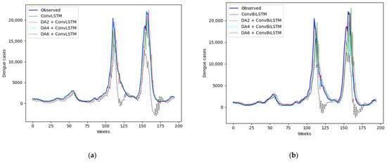
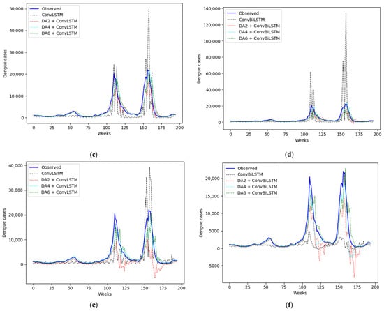
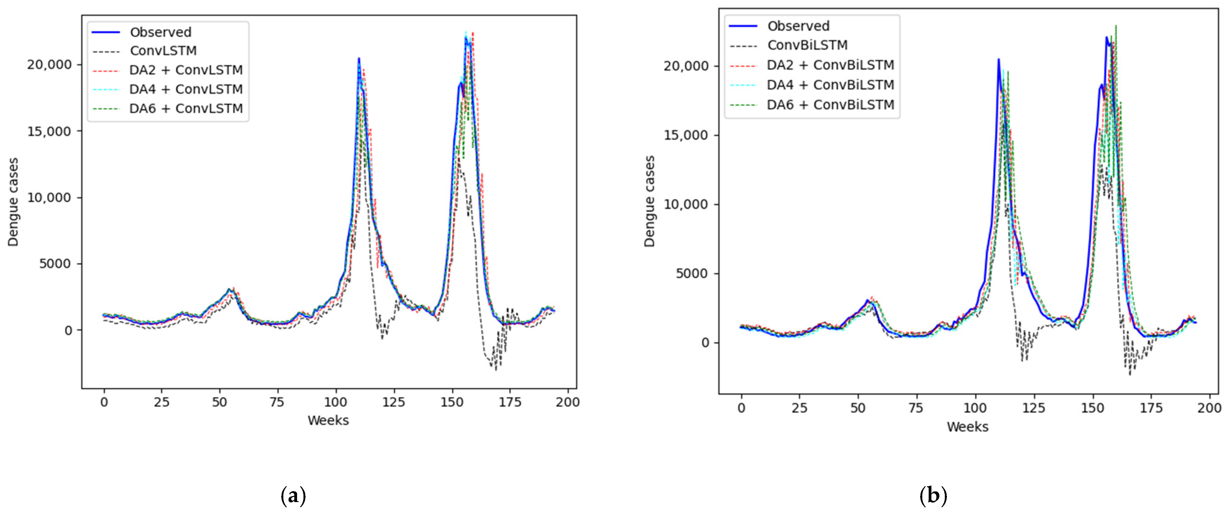
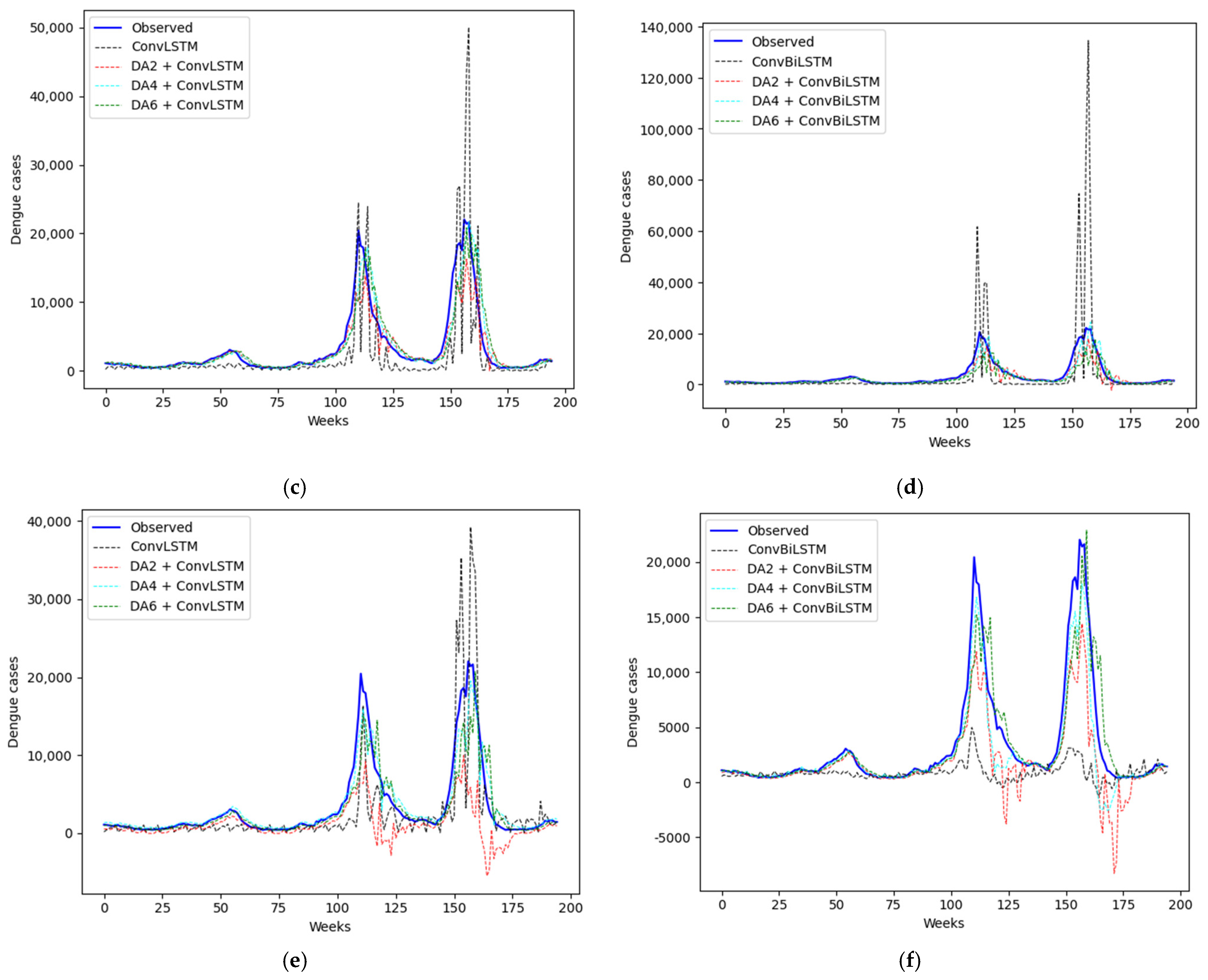
According to Figure 6, the graphical results confirm what was described in the previous tables: both models without data augmentation exhibit the poorest performance. For two-step forecasting, the best results are obtained with the ConvLSTM model using four synthetic values; as shown in Figure 6a, the cyan curve overlaps more closely with the observed data. For four-step forecasting, similar to the previous case, ConvLSTM outperforms ConvBiLSTM, with four being the optimal number of synthetic items. Finally, for six-step forecasting, as in the previous cases, ConvLSTM again achieves better results than ConvBiLSTM, with four synthetic items being the optimal amount.

Figure 6. Predictions of the implemented models with different levels of data augmentation: zero, two, four, and six synthetic items. (a) ConvLSTM for two-step forecasting (b) ConvBiLSTM for two-step forecasting, (c) ConvLSTM for four-step forecasting, (d) ConvBiLSTM for four-step forecasting, (e) ConvLSTM for six-step forecasting, and (f) ConvBiLSTM for six-step forecasting.

Regarding result stability, all reported metrics correspond to a single chronological train–validation–test split and one training run per model. Confidence intervals and repeated runs with different random seeds were not included in the current experimental setup.

As a consequence, the reported performance gains should be interpreted as indicative rather than definitive. Future work will incorporate repeated experiments with multiple random seeds and the reporting of variability measures (e.g., mean ± standard deviation or confidence intervals) to provide a more robust assessment of model stability.

4.2. Discussions

4.2.1. Comparison with Benchmark Models

The benchmark models implemented in this study include LSTM, BiLSTM, GRU, and BiGRU, all of them evaluated with and without the use of data augmentation.

Regarding baseline selection, the experimental comparison focuses primarily on recurrent neural network architectures (LSTM, BiLSTM, GRU, and BiGRU), which are widely adopted benchmarks in epidemiological time series forecasting. This choice allows for a controlled evaluation of the proposed data augmentation strategies and 2D input representations under comparable deep learning frameworks.

Classical statistical models such as ARIMA or SARIMA, as well as machine learning approaches like Prophet or XGBoost, were not included in the current experimental setup. While these methods are strong baselines in many forecasting tasks, they are typically designed for univariate or low-dimensional inputs and do not natively exploit the spatiotemporal correlations induced by the proposed 2D data formatting.

Nevertheless, we acknowledge that including a broader set of statistical and machine learning baselines would further strengthen the empirical evaluation. This will be addressed in future work to provide a more comprehensive assessment across heterogeneous forecasting paradigms.

Data augmentation is implemented by applying time warping, which increases the length of the time series by inserting synthetic elements between each pair of values in the original time series. The numbers of synthetic data points are 2, 4, and 6, and the augmentation technique used is linear interpolation, as shown in Figure 1a.

LSTM is a recurrent neural network architecture tailored for time series modeling, specifically designed to mitigate the vanishing gradient problem by incorporating a memory mechanism that selectively preserves or discards information through input, forget, and output gates.

BiLSTM extends the standard LSTM by capturing temporal dependencies in both forward and backward directions. It consists of two LSTM networks that process the sequence in opposite temporal orders, whose outputs are subsequently merged.

GRU is a recurrent neural network closely related to LSTM but characterized by a more compact and computationally efficient structure, employing only two gating mechanisms: the reset gate and the update gate.

BiGRU further extends the GRU architecture by enabling bidirectional sequence processing, allowing the model to exploit both past and future contextual information.

The hyperparameters used to implement the benchmark models are detailed in Table 7.

Table 7. Hyperparameters of the benchmark models.

Model	Hyperparameters
LSTM	[100, 50, n *], droprate: 0.2, 0.2, learning rate: 0.001
BiLSTM	[100, 50, n *], droprate: 0.2, 0.2, learning rate: 0.001
GRU	[100, 50, n *], droprate: 0.2, 0.2, learning rate: 0.001
BiGRU	[100, 50, n *], droprate: 0.2, 0.2, learning rate: 0.001

* n corresponds to the prediction steps 2, 4, or 6.

All the implemented benchmark models used the same number of layers and neurons in each layer. They were implemented in the Jupyter IDE using the TensorFlow 2.18.0 library in Python language. The lookback for each model is 12 weeks. The models were compiled with ‘mse’ as the loss function and ‘adam’ as the optimizer, with a batch size of 50 and 50 training epochs. The results achieved are shown and described below.

According to Table 8, in terms of RMSE, for the two-, four-, and six-step prediction horizons, the best-performing model for predicting weekly dengue cases is one of the models proposed in this study, namely DA4 + ConvLSTM, achieving RMSE values of 300.1274, 1092.9905, and 1473.1882 cases, respectively, outperforming all baseline models as well as the other proposed model, DA4 + ConvBiLSTM.

Table 8. Results in terms of RMSE of the Benchmark Models.

Model	Prediction Steps
	2	4	6
LSTM	1284.9484	2116.7638	2846.2583
DA2 + LSTM	743.1805	1471.4252	1954.6164
DA4 + LSTM	697.3459	1566.9055	2027.7721
DA6 + LSTM	719.4744	1624.8094	2085.0910
BiLSTM	1281.9727	1962.4873	2632.6125
DA2 +BiLSTM	737.2250	1486.1500	1931.2504
DA4 + BiLSTM	687.2845	1531.2544	2048.8066
DA6 + BiLSTM	735.8546	1598.8743	2107.9096
GRU	1136.7862	1958.8743	2739.5901
DA2 + GRU	713.4341	1459.4481	5872.3692
DA4 + GRU	1570.2819	1575.6557	1981.6978
DA6 + GRU	705.2032	1592.9134	2111.2799
BiGRU	1020.8676	1979.1655	3003.5299
DA2 + BiGRU	651.9660	1524.9624	1956.0161
DA4 + BiGRU	1515.4953	1549.9499	1963.6117
DA6 + BiGRU	713.8828	1532.1869	2121.6923
DA4 + ConvLSTM	300.1274	1092.9905	1473.1882
DA4 + ConvBiLSTM	1861.0425	1481.4508	2068.3653

The best baseline models are as follows: for the two-step prediction horizon, BiLSTM with four synthetic items (DA4 + BiLSTM) with an RMSE of 687.2845 cases; for the four-step prediction horizon, LSTM with two synthetic items (DA2 + LSTM) with an RMSE of 1471.4252 cases; and for the six-step prediction horizon, BiLSTM with two synthetic items (DA2 + BiLSTM) with an RMSE of 1931.2504 cases. All these baseline models are outperformed by the proposed DA4 + ConvLSTM model.

According to Table 9, in terms of MAPE, for the two-step prediction horizon, the best-performing model is the one proposed in this study, DA4 + ConvLSTM, achieving a MAPE of 6.81%. For the four-step prediction horizon, the best model is a baseline model, DA2 + BiLSTM, with a MAPE of 14.74%, followed by another baseline model, DA4 + BiLSTM, with a MAPE of 15.02%, and, in third place, the model proposed in this study, DA4 + ConvBiLSTM, with a MAPE of 15.31%. Finally, for the six-step prediction horizon, the best-performing model is the one proposed in this study, DA4 + ConvBiLSTM, achieving a MAPE of 25.12% and outperforming all baseline models.

Table 9. Results in terms of MAPE of the Benchmark Models.

Model	Prediction Steps
	2	4	6
LSTM	17.19	25.42	30.15
DA2 + LSTM	9.20	20.92	28.22
DA4 + LSTM	8.42	15.88	28.74
DA6 + LSTM	7.28	15.95	28.13
BiLSTM	17.36	20.92	32.09
DA2 +BiLSTM	8.77	14.74	28.27
DA4 + BiLSTM	8.13	15.02	27.75
DA6 + BiLSTM	9.41	15.43	28.87
GRU	13.18	19.38	31.16
DA2 + GRU	9.37	17.78	24.25
DA4 + GRU	19.81	16.10	31.47
DA6 + GRU	11.86	15.63	28.18
BiGRU	14.78	20.92	30.56
DA2 + BiGRU	10.60	19.82	30.02
DA4 + BiGRU	16.79	15.57	27.06
DA6 + BiGRU	9.30	16.06	29.97
DA4 + ConvLSTM	6.81	21.05	34.01
DA4 + ConvBiLSTM	23.45	15.31	25.12

According to Table 10, in terms of the correlation coefficient (R), similar to RMSE, the best-performing model is the one proposed in this study, DA4 + ConvLSTM, achieving R values of 0.9982, 0.9749, and 0.9665 for the two-, four-, and six-step prediction horizons, respectively. Among the baseline models, for the two-step prediction horizon, the best baseline model is DA2 + BiGRU with an R coefficient of 0.9914; for the four-step prediction horizon, the best baseline model is DA2 + BiLSTM with an R coefficient of 0.9572; and for the six-step prediction horizon, the best baseline model is DA2 + GRU with an R coefficient of 0.9425. All the best baseline models are outperformed by DA4 + ConvLSTM.

Table 10. Results in terms of R of the Benchmark Models.

Model	Prediction Steps
	2	4	6
LSTM	0.9740	0.9335	0.9226
DA2 + LSTM	0.9883	0.9539	0.9339
DA4 + LSTM	0.9897	0.9481	0.9095
DA6 + LSTM	0.9892	0.9447	0.9044
BiLSTM	0.9756	0.9297	0.9062
DA2 +BiLSTM	0.9899	0.9572	0.9229
DA4 + BiLSTM	0.9901	0.9501	0.9079
DA6 + BiLSTM	0.9893	0.9470	0.9035
GRU	0.9786	0.9374	0.9181
DA2 + GRU	0.9902	0.9602	0.9425
DA4 + GRU	0.9485	0.9480	0.9158
DA6 + GRU	0.9895	0.9462	0.9067
BiGRU	0.9795	0.9445	0.9251
DA2 + BiGRU	0.9914	0.9515	0.9196
DA4 + BiGRU	0.9506	0.9497	0.9166
DA6 + BiGRU	0.9894	0.9508	0.9038
DA4 + ConvLSTM	0.9982	0.9749	0.9665
DA4 + ConvBiLSTM	0.9468	0.9587	0.9295

Subsequently, we graphically compare the predictions of the best ConvLSTM- and ConvBiLSTM-based models with those of the best models based on recurrent neural networks, such as LSTM, BiLSTM, GRU, and BiGRU.

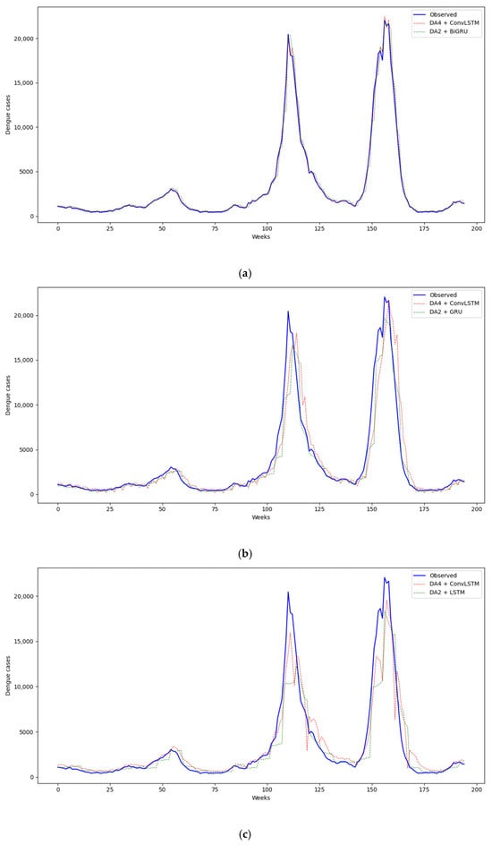
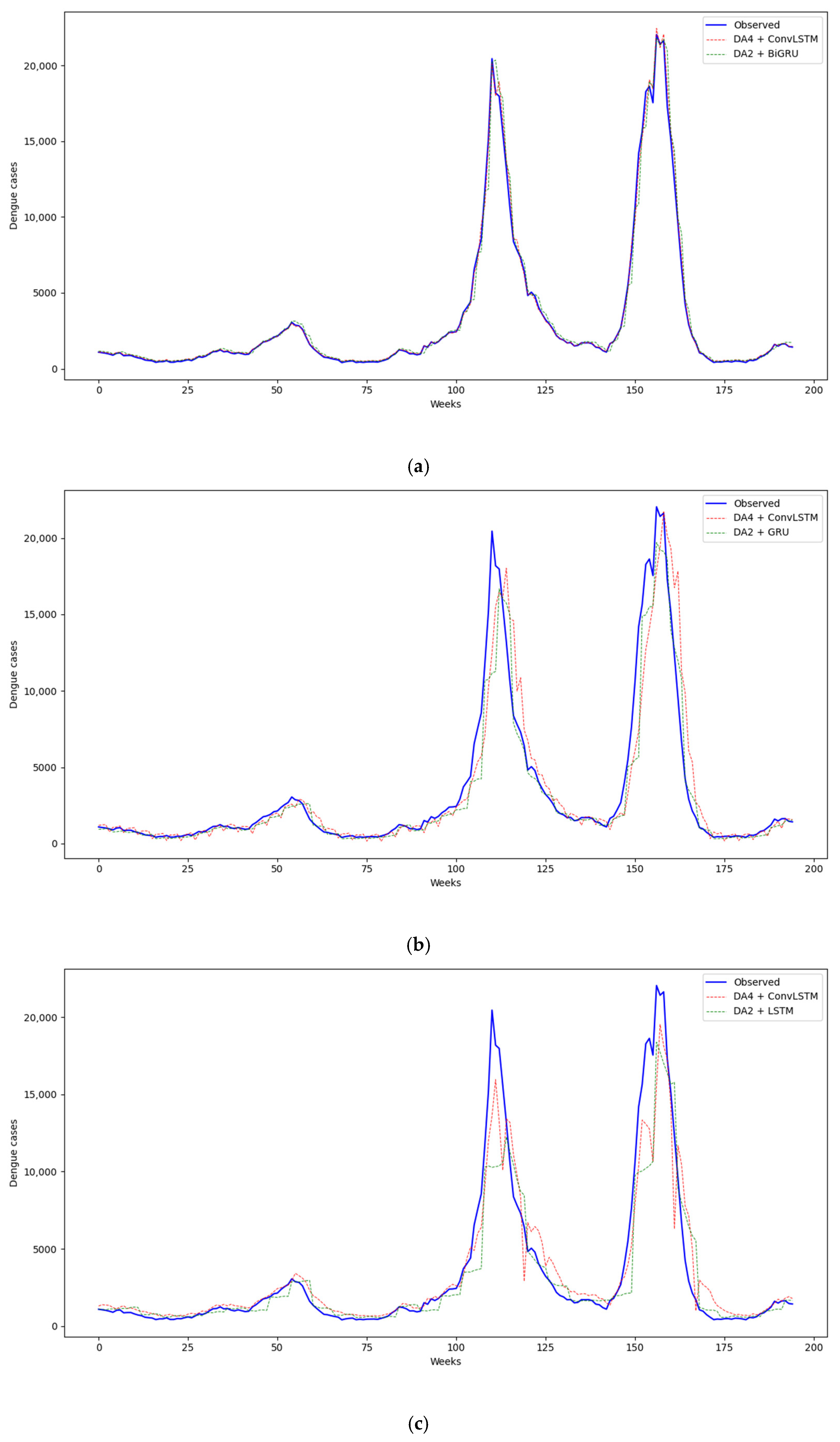
According to Figure 7, for two-step forecasting, both models achieve high predictive accuracy; however, the proposed DA4 + ConvLSTM consistently tracks the observed dengue case dynamics more closely than the strongest baseline, DA2 + BiGRU.

Figure 7. A total of 195 predicted weeks of the best proposed model vs. the best baseline model. (a) Two-step forecasting, (b) four-step forecasting, and (c) six-step forecasting.

For four-step forecasting, the performance gap between both models narrows, suggesting that mid-term predictions introduce higher uncertainty and reduce the relative advantage of short-range temporal dependencies. Nevertheless, the proposed model maintains comparable accuracy, demonstrating stable generalization as the forecasting horizon increases.

In the six-step forecasting scenario, the proposed DA4 + ConvLSTM again outperforms the baseline across most prediction segments, indicating a greater robustness to long-term temporal degradation. This is especially relevant for early outbreak monitoring, as reliable multi-week forecasts enable earlier intervention planning and resource allocation.

4.2.2. Analysis of Prediction Errors

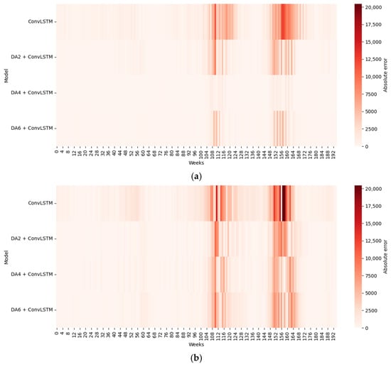
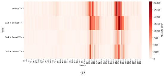
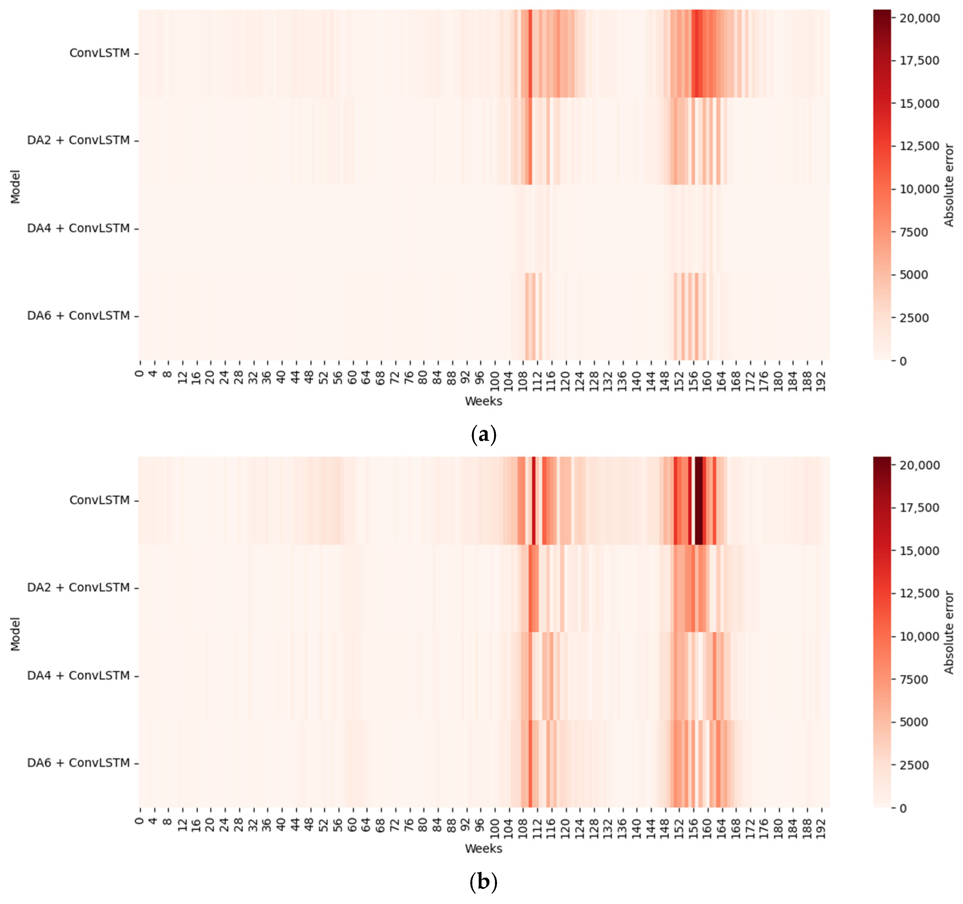
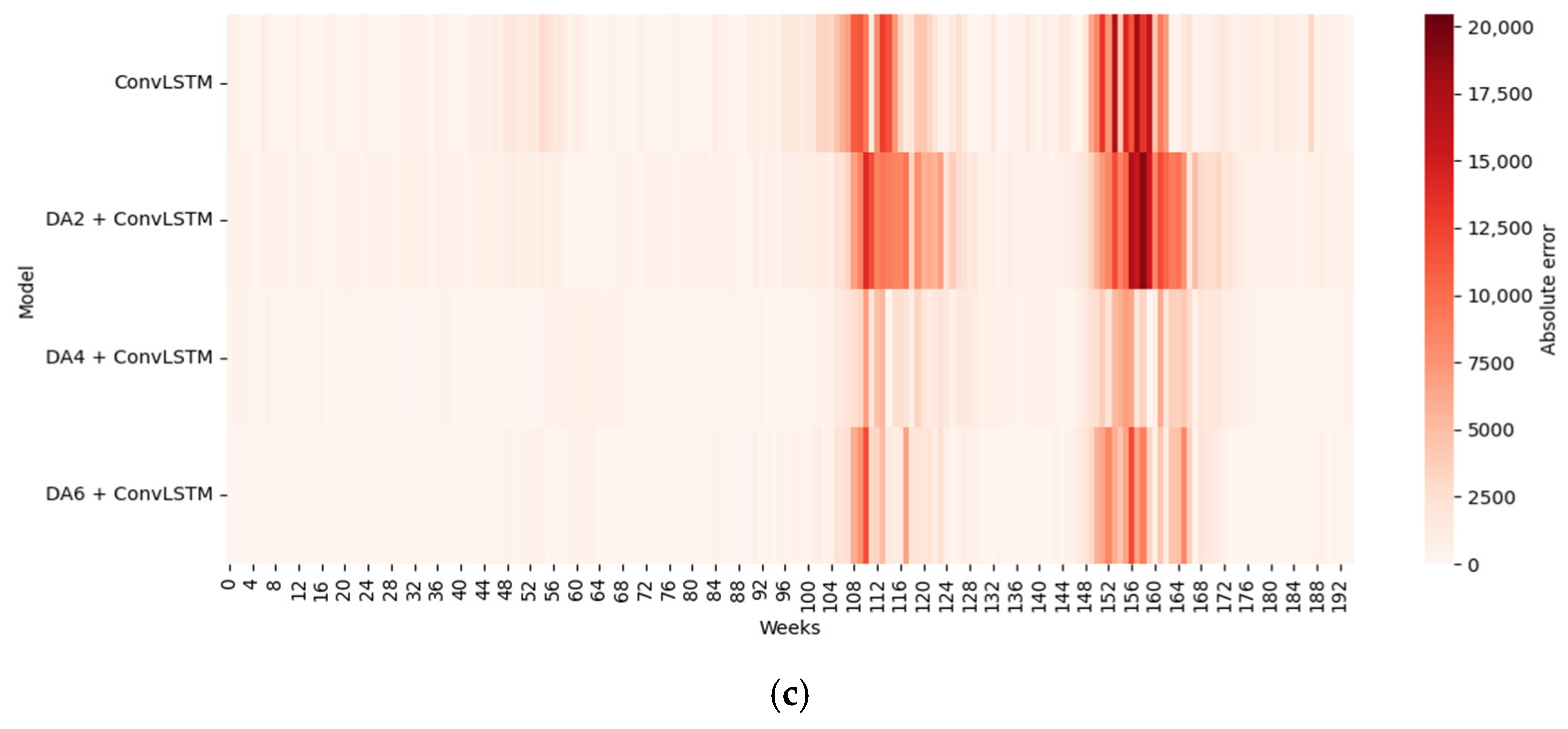
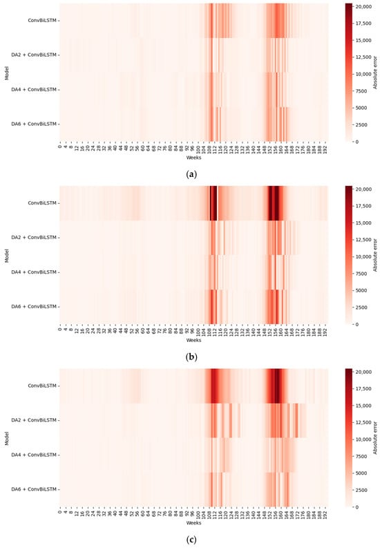
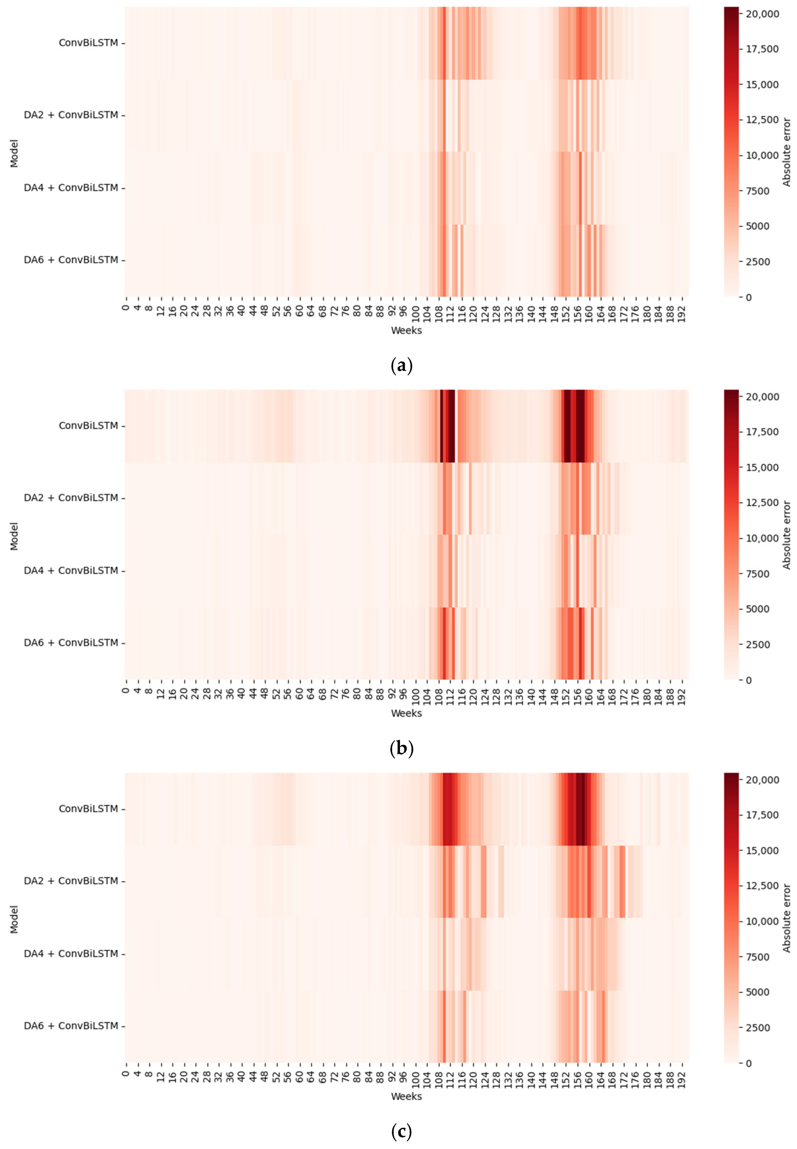
To analyze the errors in the predictions of the best proposed models, the corresponding heat maps were generated.

According to Figure 8a, for two-step forecasting, the proposed ConvLSTM-based models exhibit their highest absolute errors in two specific segments of the test set, namely between weeks 104 and 124 and weeks 150 and 172. These intervals coincide with the most extreme peaks in the observed dengue cases, as shown in Figure 6, indicating that sudden outbreaks remain the most challenging scenarios for short-term forecasting.

Figure 8. Heatmaps of proposed model ConvLSTM in test data. (a) two-step forecasting, (b) four-step forecasting, and (c) six-step forecasting.

Among all variants, the proposed DA4 + ConvLSTM model shows a noticeably lower error intensity in these high-variability segments, suggesting that the incorporation of four synthetic samples through data augmentation improves the model’s ability to learn extreme temporal patterns. This results in a more accurate representation of outbreak peaks, which are critical for early warning systems.

Figure 8b shows that for four-step forecasting, a similar error distribution pattern is preserved, with the largest errors again concentrated in the same extreme-value segments. However, the magnitude of these errors increases, reflecting the accumulation of uncertainty as the forecasting horizon expands. Despite this increase, DA4 + ConvLSTM continues to outperform the other variants, demonstrating greater robustness to mid-term temporal degradation. Notably, in this setting, DA2 + ConvLSTM becomes the worst-performing model, suggesting that limited data augmentation is insufficient to mitigate error propagation at longer horizons.

Finally, Figure 8c illustrates that for six-step forecasting, the error hotspots remain localized in the same outbreak periods, confirming that extreme dengue peaks dominate long-horizon prediction errors. Once again, DA4 + ConvLSTM achieves the lowest overall error intensity, highlighting its superior generalization capability under highly variable conditions. This behavior is particularly relevant for public health decision-making, as reliable multi-week forecasts during outbreak periods enable earlier intervention planning and more effective resource allocation.

According to Figure 9a, for two-step forecasting, the ConvBiLSTM-based models exhibit their highest absolute errors in the same outbreak-related segments previously identified for ConvLSTM, confirming that extreme dengue peaks remain the most challenging events to predict regardless of the recurrent architecture. In this short-term setting, DA2 + ConvBiLSTM achieves the lowest error intensity, suggesting that a moderate level of data augmentation is sufficient for the bidirectional architecture to effectively capture short-range temporal dependencies.

Figure 9. Heatmaps of proposed model ConvBiLSTM in test data. (a) Two-step forecasting, (b) four-step forecasting, and (c) six-step forecasting.

Figure 9b shows that for four-step forecasting, error concentrations persist in the same high-variability segments; however, DA4 + ConvBiLSTM outperforms the other variants. This indicates that as the forecasting horizon increases, additional synthetic samples become necessary to compensate for error propagation and to maintain stable bidirectional temporal representations. In contrast, the baseline ConvBiLSTM model consistently exhibits the poorest performance, highlighting its limited generalization capability when trained without data augmentation.

Finally, Figure 9c demonstrates that for six-step forecasting, the error distribution remains dominated by the same outbreak periods, reinforcing the notion that long-horizon forecasting accuracy is primarily constrained by extreme case dynamics. Once again, DA4 + ConvBiLSTM delivers the best overall performance, confirming that stronger data augmentation enhances the robustness of bidirectional models under highly variable conditions. From a practical perspective, this robustness is crucial for multi-week dengue outbreak preparedness and early response planning.

In summary, the error analysis reveals that the largest prediction errors consistently occur during peak outbreak weeks, which represent the most critical periods for public health decision-making. These peaks are characterized by abrupt, nonlinear increases in dengue cases, often driven by complex interactions between climatic conditions, vector dynamics, and human mobility, which are difficult to fully capture using historical case data alone.

Although the proposed models significantly reduce overall error and improve performance relative to baseline approaches, residual inaccuracies during peak weeks indicate that forecasting extreme outbreak magnitudes remains a challenging task. From a public health perspective, these errors may affect the precise estimation of peak intensity; however, the models still provide valuable early signals regarding the timing and onset of outbreak periods.

Importantly, the ability to anticipate the rising phase of an outbreak several weeks in advance enables authorities to initiate vector control measures, allocate healthcare resources, and implement preventive campaigns, even if the exact peak magnitude is not perfectly predicted. Therefore, the proposed models should be interpreted as decision-support tools for early warning rather than exact peak quantification mechanisms.

Future work will focus on improving peak prediction accuracy by incorporating additional exogenous variables, adaptive loss functions that emphasize extreme values, and probabilistic forecasting frameworks to better quantify uncertainty during outbreak periods.

4.2.3. Statistical Analysis

Statistical analysis was conducted to compare the distributions of forecasting errors using the Kolmogorov–Smirnov (KS) test. The KS test was employed as a non-parametric tool to assess whether the error distributions of different models differ significantly, without assuming a specific error distribution.

It is important to note that the KS test evaluates distributional differences rather than directly testing predictive accuracy superiority. Therefore, the statistical results should be interpreted as complementary to the performance metrics (RMSE, R, and MAPE), rather than as definitive evidence of model dominance.

For forecasting horizons where the reported p-values exceed the 0.05 significance level, no statistically significant difference between models can be concluded, even if one model exhibits lower average error values. In such cases, performance differences are discussed in descriptive rather than inferential terms.

To determine whether one model is significantly different than another, in this section the Kolmogorov–Smirnov (KS) test for two samples was applied. This test determines whether there is a significant difference between the proposed models and the benchmark models.

According to Table 11, it can be observed that only for six-step forecasting—where the best benchmark model is DA2 + LSTM—the p-value is lower than 0.05, indicating that only in this case the DA4 + ConvLSTM model is significantly different to the baseline model. For two prediction steps, the p-value is far from 0.05; therefore, in this case, the proposed model is not significantly different to the baseline model. Finally, for four prediction steps, the p-value is closer to 0.05; however, it is still not below this threshold, and thus it cannot be stated that the proposed model is significantly different to the baseline model.

Table 11. p-values for Kolmogorov–Smirnov (KS) test between DA4 + ConvLSTM and the best benchmark models.

Model	Prediction Steps
	2	4	6
DA2 + LSTM	-	-	0.0020
DA2 + GRU	-	0.0811	-
DA2 + BiGRU	0.9166	-	-

According to Table 12, unlike the ConvLSTM model, ConvBiLSTM achieves p-values lower than 0.05 for two prediction horizons, namely two and six steps, indicating that its results for these horizons are significantly different to those of the best benchmark models. Only for the four-step prediction horizon is a p-value greater than 0.05 obtained; therefore, in this case, the results of the proposed ConvBiLSTM model are not significantly different to the benchmark models.

Table 12. p-values for Kolmogorov–Smirnov (KS) test between DA4 + ConvBiLSTM and the best benchmark models.

Model	Prediction Steps
	2	4	6
DA2 + LSTM	-	-	0.0001
DA2 + GRU	-	0.6124	-
DA2 + BiGRU	0.0012	-	-

4.2.4. Computational Cost, Latency and Memory Usage

Table 13 shows the computational cost required to train each of the models implemented in this study, including the proposal model, on a computer with a HP Boeblingen Germany Core i7-13700H processor at 2.40 GHz, 16 GB of RAM, running on a Windows 11 environment.

Table 13. Computational cost of the implemented models in seconds.

Model	Prediction Steps
	2	4	6	Avg
ConvLSTM	13.1737	8.7206	7.4374	9.7772
DA2 + ConvLSTM	28.8617	17.5682	12.1639	19.5313
DA4 + ConvLSTM	47.7088	26.4754	19.1006	31.0949
DA6 + ConvLSTM	65.4445	35.3497	25.1865	41.9936
ConvBiLSTM	17.2780	11.4644	9.6043	12.7822
DA2 + ConvBiLSTM	39.0698	24.1147	17.4642	26.8829
DA4 + ConvBiLSTM	63.8184	36.9999	25.1750	41.9978
DA6 + ConvBiLSTM	89.5714	47.4100	34.9818	57.3211
LSTM	10.6364	12.7508	11.1542	11.5138
DA2 + LSTM	39.2458	45.1923	44.0813	42.8398
DA4 + LSTM	36.3283	35.2239	34.2699	35.2740
DA6 + LSTM	46.9361	47.7697	49.3969	48.0342
BiLSTM	14.2455	15.5279	14.4924	14.7553
DA2 + BiLSTM	57.9414	60.9752	63.0423	60.6530
DA4 + BiLSTM	47.2531	48.5852	45.6388	47.1590
DA6 + BiLSTM	63.4513	63.1793	63.6762	63.4356
GRU	11.2624	12.5080	11.0987	11.6230
DA2 + GRU	49.3312	48.2093	47.1358	48.2254
DA4 + GRU	36.3114	36.0566	37.2010	36.5230
DA6 + GRU	49.7547	48.1168	50.4222	49.4312
BiGRU	15.7145	17.0654	17.4967	16.7589
DA2 + BiGRU	64.5018	63.7472	71.1936	66.4809
DA4 + BiGRU	54.7155	51.9757	53.4051	53.3654
DA6 + BiGRU	73.9738	74.0948	73.2915	73.7867

According to Table 13, the training costs in seconds of the different implemented models, including the proposed models and the benchmark models, can be observed. On average, the model with the lowest training cost is ConvLSTM, both without and with data augmentation across all levels of synthetic data, namely 2, 4, and 6. For 0 synthetic items, the average training time is 9.7772 s; for two synthetic items, it is 19.5313 s; for four synthetic items, it is 31.0949 s; and for six synthetic items, it is 41.9936 s. This demonstrates that, despite the complexity of the ConvLSTM model, its training time does not increase disproportionately and remains lower than that required to train other state-of-the-art models both without and with data augmentation.

According to Table 14, the latency of the implemented models for predicting the total number of items in the test subset is shown.

Table 14. Latency of the implemented models in seconds.

Model	Prediction Steps
	2	4	6	Avg
ConvLSTM	0.0669	0.0575	0.0494	0.0579
DA2 + ConvLSTM	0.0754	0.0713	0.0697	0.0721
DA4 + ConvLSTM	0.0942	0.0692	0.0687	0.0774
DA6 + ConvLSTM	0.1078	0.0796	0.0853	0.0909
ConvBiLSTM	0.0613	0.0594	0.0531	0.0579
DA2 + ConvBiLSTM	0.0989	0.0644	0.0671	0.0768
DA4 + ConvBiLSTM	0.0943	0.0787	0.0695	0.0808
DA6 + ConvBiLSTM	0.1285	0.0866	0.0910	0.1020
LSTM	0.0648	0.0646	0.0648	0.0647
DA2 + LSTM	0.0918	0.0901	0.0845	0.0888
DA4 + LSTM	0.3221	0.2966	0.1093	0.2427
DA6 + LSTM	0.4167	0.3138	0.3648	0.3651
BiLSTM	0.0690	0.0619	0.0630	0.0646
DA2 + BiLSTM	0.0979	0.0978	0.0972	0.0976
DA4 + BiLSTM	0.3501	0.2805	0.1322	0.2543
DA6 + BiLSTM	0.3700	0.4038	0.4811	0.4183
GRU	0.0626	0.0671	0.0633	0.0643
DA2 + GRU	0.0896	0.0852	0.0863	0.0870
DA4 + GRU	0.3098	0.3055	0.2507	0.2887
DA6 + GRU	0.3298	0.4715	0.2793	0.3602
BiGRU	0.0621	0.0557	0.0665	0.0614
DA2 + BiGRU	0.0949	0.0946	0.0962	0.0952
DA4 + BiGRU	0.4068	0.3672	0.1277	0.3006
DA6 + BiGRU	0.3998	0.3711	0.3527	0.3745

On average, without data augmentation, the ConvLSTM and ConvBiLSTM models exhibit the lowest latency, both with 0.0579 s. Among the benchmark models without data augmentation, BiGRU shows the lowest latency at 0.0614 s.

On average, with data augmentation, it is observed that all models, without exception, increase their latency as the number of synthetic data points increases. As in the case without data augmentation, the models that exhibit the smallest latency increase are those proposed in this study; however, in this case, the difference with respect to the benchmark models becomes more pronounced, especially when the number of synthetic values is four and six.

Among the two proposed models, across all levels of synthetic values, ConvLSTM presents the lowest latency, with average values of 0.0721, 0.0774, and 0.0909 s for two, four, and six synthetic values, respectively. For the benchmark models, with two synthetic values, GRU shows the lowest average latency at 0.0870 s. With four synthetic values, LSTM presents the lowest average latency at 0.2427 s. Finally, for six synthetic values, GRU again exhibits the lowest average latency at 0.3602 s.

Comparing the best proposed model with the best benchmark models, for two synthetic values, there is a difference of 0.0149 s in favor of ConvLSTM with respect to GRU. For four synthetic values, there is a difference of 0.1653 s between ConvLSTM and LSTM. For six synthetic values, the difference between ConvLSTM and LSTM increases to 0.2693 s. These results indicate that the increase in data volume affects the benchmark models more severely than the proposed model.

The peak memory usage during inference was measured using Python’s tracemalloc library. The reported values correspond to the maximum heap memory allocated by Python while performing a forward pass on the test set.

According to Table 15, on average, among the proposed models, ConvLSTM requires the lowest peak memory during the inference process, showing a slight increase as the number of synthetic values increases.

Table 15. Peak memory used in MB during inference of the implemented models.

Model	Prediction Steps
	2	4	6	Avg
ConvLSTM	0.2075	0.2108	0.2056	0.2080
DA2 + ConvLSTM	0.2071	0.2043	0.2046	0.2053
DA4 + ConvLSTM	0.2061	0.2064	0.2121	0.2082
DA6 + ConvLSTM	0.2214	0.2061	0.2053	0.2109
ConvBiLSTM	0.2240	0.2336	0.2199	0.2258
DA2 + ConvBiLSTM	0.2230	0.2252	0.2211	0.2231
DA4 + ConvBiLSTM	0.2206	0.2337	0.2355	0.2299
DA6 + ConvBiLSTM	0.2354	0.2338	0.2201	0.2298
LSTM	0.2247	0.2233	0.2414	0.2298
DA2 + LSTM	0.2135	0.2409	0.2138	0.2227
DA4 + LSTM	0.2169	0.2128	0.2411	0.2236
DA6 + LSTM	0.2162	0.2769	0.2752	0.2561
BiLSTM	0.2855	0.2873	0.2508	0.2745
DA2 + BiLSTM	0.2484	0.2512	0.2419	0.2472
DA4 + BiLSTM	0.2332	0.2496	0.2616	0.2481
DA6 + BiLSTM	0.2754	0.2512	0.2332	0.2533
GRU	0.2244	0.2447	0.2256	0.2316
DA2 + GRU	0.2442	0.2167	0.2156	0.2255
DA4 + GRU	0.2162	0.2432	0.2158	0.2251
DA6 + GRU	0.2779	0.2753	0.2173	0.2568
BiGRU	0.2503	0.2606	0.2922	0.2677
DA2 + BiGRU	0.2558	0.2504	0.2507	0.2523
DA4 + BiGRU	0.2937	0.2922	0.2277	0.3006
DA6 + BiGRU	0.2461	0.2423	0.2750	0.3745

On the other hand, the benchmark models require a higher peak memory usage, with LSTM and GRU being the most memory-efficient among them. Likewise, these models exhibit an increase in memory requirements as the number of synthetic values increases, to a greater extent than the proposed models.

4.2.5. Comparison Between Proposed Models and Related Works

Comparing the results of the models implemented in this study with those reported in related works may not be entirely appropriate, as the datasets used in previous studies exhibit different characteristics, such as minimum and maximum values, dispersion, and overall variability. Nevertheless, a brief comparison is conducted by considering only studies that report the MAPE as the evaluation metric. Metrics such as RMSE, MSE, MAE, and similar ones are excluded, as they are not the most suitable for this type of analysis.

According to Table 16, the studies reporting results in terms of MAPE are [38,39,40,45,47] and they are listed in Table 15. Study [45] was excluded because the number of prediction steps reported exceeds those considered in this study. Thus, the comparative analysis is restricted to four related works that report a maximum of four prediction steps. The proposed DA4 + ConvLSTM model, with a MAPE of 21.05%, outperforms two of the four related works, namely [39,40], while it is outperformed by [38,47]. In contrast, the proposed DA4 + ConvBiLSTM model, achieving a MAPE of 15.31%, outperforms three of the four selected related works—specifically [38,39,40] —and is only outperformed by [47], which reports a MAPE of 14.62%, representing a marginal difference of 0.69%.

Table 16. Proposed models vs. related works.

Work	Country	Technique	Freq.	Step Size	Metric	Value
[45]	Singapore	LASSO	Weekly	12	MAPE	24.00
[38]	Singapore	RNN, GRU, LSTM, BiLSTM, CNN	Weekly	4	MAPE	17.89
[39]	Brazil	LSTM		4	MAPE	21.87
[47]	Singapore	BiLSTM	Weekly	4	MAPE	14.62
[40]	Brazil	LSTM	Weekly	4	MAPE	29.11
Our work	Peru	DA4 + ConvLSTM	Weekly	4	MAPE	21.05
	Peru	DA4 + ConvBiLSTM	Weekly	4	MAPE	15.31

It is worth noting that study [38] uses a dataset in which the weekly number of dengue cases does not exceed 2000 cases. Similarly, study [47] relies on a dataset where the maximum weekly dengue case count does not exceed 1750 cases. In contrast, the dataset employed in this study exhibits substantially higher variability, with a maximum of 22,038 weekly dengue cases.

4.2.6. Comparative Summary Between the Proposed Models and the Benchmark Models

The obtained results in terms of accuracy, latency, and memory usage were discretized into three performance categories (low, medium, and high) using tercile-based thresholds. Accuracy was obtained from RMSE. Table 17 shows the discretized values.

Table 17. Recommended use case of the implemented models.

Model	Accuracy	Latency	Memory Usage	Recommended Use Case
ConvLSTM	Low	Low	Low
DA2 + ConvLSTM	Low	Low	Low
DA4 + ConvLSTM	High	Low	Low	Real-time early warning systems (1°)
DA6 + ConvLSTM	Medium	Low	Low
ConvBiLSTM	Low	Low	Medium
DA2 + ConvBiLSTM	Medium	Low	Low
DA4 + ConvBiLSTM	Medium	Low	Medium
DA6 + ConvBiLSTM	Medium	Medium	Medium
LSTM	Medium	Low	Medium
DA2 + LSTM	High	Low	Low	Real-time early warning systems (2°)
DA4 + LSTM	High	Medium	Low	Offline analysis
DA6 + LSTM	High	High	High
BiLSTM	Medium	Low	High
DA2 + BiLSTM	High	Medium	Medium	Offline analysis
DA4 + BiLSTM	High	Medium	Medium	Offline analysis
DA6 + BiLSTM	High	High	Medium
GRU	Medium	Low	Medium
DA2 + GRU	Low	Low	Low
DA4 + GRU	Medium	High	Low
DA6 + GRU	High	High	High
BiGRU	Medium	Low	High
DA2 + BiGRU	High	Medium	Medium	Offline analysis
DA4 + BiGRU	Medium	High	High
DA6 + BiGRU	High	High	High

According to Table 16, based on the selected evaluation criteria, the model recommended as the primary choice for the implementation of real-time early warning systems is DA4 + ConvLSTM, as it achieved the best categories across the considered criteria—High, Low, and Low for accuracy, latency, and memory usage, respectively. In terms of accuracy, it ranked first (955.4355); for latency, it ranked eighth (0.0774); and for memory usage, it ranked third (0.2082).

The second model also recommended is DA2 + LSTM, which, similar to the previous model, achieved the best categories across all criteria. In terms of accuracy, it ranked fourth (1389.7407); for latency, it ranked twelfth (0.0888); and for memory usage, it ranked sixth (0.2227).

4.2.7. Limitations

• Study limitations

This study is subject to several limitations. First, only historical weekly dengue case data were considered, resulting in the implementation of univariate models. While this setting is appropriate for scenarios with limited data availability, it may restrict the ability to capture the influence of external factors. Second, the analysis was limited to dengue cases in Peru, which may affect the generalizability of the findings to other epidemiological contexts. Future work should evaluate the proposed framework using additional datasets and data from different countries.

• Proposed approach limitations

From a methodological perspective, this study also presents some limitations.

Only a single interpolation technique—namely linear interpolation—was evaluated as a data augmentation strategy for both the proposed and benchmark models. Future studies should investigate alternative interpolation and data augmentation techniques to further assess their impact on predictive performance.

The use of fixed architectural hyperparameters across models may not fully exploit the optimal capacity of each architecture. Future work will explore architecture-specific hyperparameter optimization using grid search or Bayesian optimization.

This study does not include transformer-based or TCN architectures. Future work will extend the proposed data augmentation framework to these models to assess its generalizability across different forecasting paradigms.

The statistical analysis relies on the KS test, which evaluates differences between error distributions but is not specifically designed for forecast accuracy comparison. Future studies will incorporate dedicated forecasting comparison tests, such as the Diebold–Mariano test, to strengthen inferential conclusions.

Moreover, the proposed models were restricted to architectures available within the TensorFlow 2.18.0 library. Future work could explore additional deep learning architectures, such as ConvGRU, ConvBiGRU, and related variants.

5. Conclusions

According to the obtained results, it is observed that the proposed ConvLSTM and ConvBiLSTM models with data augmentation—specifically DA4 + ConvLSTM and DA4 + ConvBiLSTM—were not statistically significantly different to the benchmark models across all prediction steps; however, they were significantly different for the largest prediction horizon, namely six steps. In addition, these models demonstrated superior predictive performance across different metrics, such as RMSE, MAPE, and the correlation coefficient R, compared to most benchmark models. Therefore, it can be concluded that DA4 + ConvLSTM constitutes excellent alternative for multi-step forecasting of weekly dengue cases showing high accuracy, low latency and low memory usage.

References

- Shafie, A.A.; Moreira, E.D.; Di Pasquale, A.; Demuth, D.; Yin, J.Y.S. Knowledge, Attitudes and Practices toward Dengue Fever, Vector Control, and Vaccine Acceptance Among the General Population in Countries from Latin America and Asia Pacific: A Cross-Sectional Study (GEMKAP). Vaccines 2023, 11, 575. [Google Scholar] [CrossRef] [Scilit]
- Liu, Z.; Zhang, Q.; Li, L.; He, J.; Guo, J.; Wang, Z.; Huang, Y.; Xi, Z.; Yuan, F.; Li, Y.; et al. The effect of temperature on dengue virus transmission by Aedes mosquitoes. Front. Cell. Infect. Microbiol. 2023, 13, 1242173. [Google Scholar] [CrossRef] [Scilit]
- Rocklöv, J.; Tozan, Y. Climate change and the rising infectiousness of dengue. Emerg. Top. Life Sci. 2019, 3, 133–142. [Google Scholar] [CrossRef] [Scilit]
- Mandal, A.; Debnath, P.; Das, P.; Ghosh, D. A climate-driven mechanistic model of dengue transmission: Linking entomological processes to epidemiological dynamics. Chaos Solitons Fractals 2026, 204, 117818. [Google Scholar] [CrossRef] [Scilit]
- Li, Y.; An, Q.; Sun, Z.; Gao, X.; Wang, H. Distribution areas and monthly dynamic distribution changes of three Aedes species in China: Aedes aegypti, Aedes albopictus and Aedes vexans. Parasites Vectors 2023, 16, 297. [Google Scholar] [CrossRef] [Scilit]
- Ismail, S.; Fildes, R.; Ahmad, R.; Wan Mohamad Ali, W.N.; Omar, T. The practicality of Malaysia dengue outbreak forecasting model as an early warning system. Infect. Dis. Model. 2022, 7, 510–525. [Google Scholar] [CrossRef] [Scilit]
- Moishin, M.; Deo, R.C.; Prasad, R.; Raj, N.; Abdulla, S. Designing deep-based learning flood forecast model with ConvLSTM hybrid algorithm. IEEE Access 2021, 9, 50982–50993. [Google Scholar] [CrossRef] [Scilit]
- Tam, S.; Said, R.B.; Tanriöver, Ö. A ConvBiLSTM Deep Learning Model-Based Approach for Twitter Sentiment Classification. IEEE Access 2021, 9, 41283–41293. [Google Scholar] [CrossRef] [Scilit]
- Sepp Hochreiter, J.S. Long Short-Term Memory. Neural Comput. 1997, 9, 1735–1780. [Google Scholar] [CrossRef] [Scilit] [PubMed]
- Li, C.; Denison, T.; Zhu, T. A Survey of Few-Shot Learning for Biomedical Time Series. IEEE Rev. Biomed. Eng. 2025, 18, 192–210. [Google Scholar] [CrossRef] [Scilit] [PubMed]
- Flores, A.; Tito-Chura, H.; Yana-Mamani, V.; Rosado-Chavez, C.; Ecos-Espino, A. Weighted Averages and Polynomial Interpolation for PM2.5 Time Series Forecasting. Computers 2024, 13, 238. [Google Scholar] [CrossRef] [Scilit]
- Flores, A.; Tito-Chura, H.; Guzman-Valdivia, J.; Morales-Gonzales, R.; Flores-Quispe, E.; Cuentas-Toledo, O. A Multi-Step PM2.5 Time Series Forecasting Approach for Mining Areas Using Last Day Observed, Correlation-Based Retrieval, and Interpolation. Computers 2025, 14, 471. [Google Scholar] [CrossRef] [Scilit]
- Fard, S.G.; Rahimi, H.M.; Motie, P.; Minabi, M.A.S.; Taheri, M.; Nateghinia, S. Application of machine learning in the prediction of COVID-19 daily new cases: A scoping review. Heliyon 2021, 7, e08143. [Google Scholar] [CrossRef] [Scilit]
- Zhang, L.; Liu, P.; Zhao, L.; Wang, G.; Zhang, W.; Liu, J. Air quality predictions with a semi-supervised bidirectional LSTM neural network. Atmos. Pollut. Res. 2021, 12, 328–339. [Google Scholar] [CrossRef] [Scilit]
- Pan, M.; Zhou, H.; Cao, J.; Liu, Y.; Hao, J.; Li, S.; Chen, C.H. Water Level Prediction Model Based on GRU and CNN. IEEE Access 2020, 8, 60090–60100. [Google Scholar] [CrossRef] [Scilit]
- Zhang, Z.; Dong, Z.; Lin, H.; He, Z.; Wang, M.; He, Y.; Gao, X.; Gao, M. An Improved Bidirectional Gated Recurrent Unit Method for Accurate State-of-Charge Estimation. IEEE Access 2021, 9, 11252–11263. [Google Scholar] [CrossRef] [Scilit]
- Iglesias, G.; Talavera, E.; González-Prieto, Á.; Mozo, A.; Gómez-Canaval, S. Data Augmentation techniques in time series domain: A survey and taxonomy. Neural Comput. Appl. 2023, 35, 10123–10145. [Google Scholar] [CrossRef] [Scilit]
- Jeong, C.Y.; Shin, H.C.; Kim, M. Sensor-data augmentation for human activity recognition with time-warping and data masking. Multimed. Tools Appl. 2021, 80, 20991–21009. [Google Scholar] [CrossRef] [Scilit]
- Iwana, B.K.; Uchida, S. An empirical survey of data augmentation for time series classification with neural networks. PLoS ONE 2021, 16, e0254841. [Google Scholar] [CrossRef] [Scilit]
- Flores, A.; Tito-Chura, H.; Apaza-Alanoca, H. Data Augmentation for Short-Term Time Series Prediction with Deep Learning. In Proceedings of the Lecture Notes in Networks and Systems; Springer: Berlin/Heidelberg, Germany, 2021; Volume 284. [Google Scholar]
- Li, J.; Yin, K.; Tang, C. Slideaugment: A simple data processing method to enhance human activity recognition accuracy based on wifi. Sensors 2021, 21, 2181. [Google Scholar] [CrossRef] [Scilit]
- Rashid, K.M.; Louis, J. Window-warping: A time series data augmentation of IMU data for construction equipment activity identification. In Proceedings of the 36th International Symposium on Automation and Robotics in Construction, ISARC 2019, Banff, AB, Canada, 21–24 May 2019. [Google Scholar]
- Zhang, J.; Chen, J.; Deng, H.; Hu, W. A novel framework based on adaptive Multi-Task learning for bearing fault diagnosis. Energy Rep. 2023, 9, 522–531. [Google Scholar] [CrossRef] [Scilit]
- Eslami, T.; Mirjalili, V.; Fong, A.; Laird, A.R.; Saeed, F. ASD-DiagNet: A Hybrid Learning Approach for Detection of Autism Spectrum Disorder Using fMRI Data. Front. Neuroinform. 2019, 13, 70. [Google Scholar] [CrossRef] [Scilit]
- Flores, A.; Valeriano-Zapana, J.; Yana-Mamani, V.; Tito-chura, H. PM2.5 prediction with Recurrent Neural Networks and Data Augmentation. In Proceedings of the 2021 IEEE Latin American Conference on Computational Intelligence; IEEE: Temuco, Chile, 2021. [Google Scholar]
- Haus, B.; Mercorelli, P. Polynomial Augmented Extended Kalman Filter to Estimate the State of Charge of Lithium-Ion Batteries. IEEE Trans. Veh. Technol. 2020, 69, 1452–1463. [Google Scholar] [CrossRef] [Scilit]
- Abayomi-Alli, O.O.; Damasevicius, R.; Maskeliunas, R.; Abayomi-Alli, A. BiLSTM with Data Augmentation using Interpolation Methods to Improve Early Detection of Parkinson Disease. In Proceedings of the 2020 Federated Conference on Computer Science and Information Systems, FedCSIS 2020, Sofia, Bulgaria, 7–9 September 2020; Volume 21. [Google Scholar]
- Saleh, A.Y.; Baiwei, L. Dengue prediction using deep learning with long short-term memory. In Proceedings of the 2021 1st International Conference on Emerging Smart Technologies and Applications, eSmarTA 2021, Sana’a, Yemen, 10–12 August 2021. [Google Scholar]
- Ligue, K.D.B.; Ligue, K.J.B. Deep Learning Approach to Forecasting Dengue Cases in Davao City Using Long Short-term Memory (LSTM). Philipp. J. Sci. 2022, 151, 797. [Google Scholar] [CrossRef] [Scilit]
- Majeed, M.A.; Shafri, H.Z.M.; Wayayok, A.; Zulkafli, Z. Prediction of dengue cases using the attention-based long short-term memory (LSTM) approach. Geospat. Health 2023, 18. [Google Scholar] [CrossRef] [Scilit] [PubMed]
- Zhang, Z.; Hu, S.; Hu, J.; Hao, Z.; Huang, J. Decoding multi-frequency scale climate-dengue dynamics: An interpretable modeling framework. Urban Clim. 2026, 65, 102734. [Google Scholar] [CrossRef] [Scilit]
- Bunprom, P.; Siramaneerat, I.; Bhumkittipich, P. Forecasting Dengue Fever Incidence in Thailand Using ARIMA: Implications for Public Health Planning. Environ. Nat. Resour. J. 2026, 24, 88–97. [Google Scholar] [CrossRef] [Scilit]
- Liu, B.; Hossain, M.F.; Hossain, S. A comparative evaluation of multiple machine learning approaches for forecasting dengue outbreaks in Bangladesh. Sci. Rep. 2025, 15, 35931. [Google Scholar] [CrossRef] [Scilit]
- Mobin, M. Al Multivariate forecasting of dengue infection in Bangladesh: Evaluating the influence of data downscaling on machine learning predictive accuracy. BMC Infect. Dis. 2025, 25, 761. [Google Scholar] [CrossRef] [Scilit]
- Sebastianelli, A.; Spiller, D.; Carmo, R.; Wheeler, J.; Nowakowski, A.; Jacobson, L.V.; Kim, D.; Barlevi, H.; Cordero, Z.E.R.; Colón-González, F.J.; et al. A reproducible ensemble machine learning approach to forecast dengue outbreaks. Sci. Rep. 2024, 14, 3807. [Google Scholar] [CrossRef] [Scilit]
- Chen, X.; Moraga, P. Assessing dengue forecasting methods: A comparative study of statistical models and machine learning techniques in Rio de Janeiro, Brazil. Trop. Med. Health 2025, 53, 52. [Google Scholar] [CrossRef] [Scilit]
- Xu, J.; Xu, K.; Li, Z.; Meng, F.; Tu, T.; Xu, L.; Liu, Q. Forecast of dengue cases in 20 chinese cities based on the deep learning method. Int. J. Environ. Res. Public Health 2020, 17, 453. [Google Scholar] [CrossRef] [Scilit]
- Zhao, X.; Li, K.; Ang, C.K.E.; Cheong, K.H. A deep learning based hybrid architecture for weekly dengue incidences forecasting. Chaos Solitons Fractals 2023, 168, 113170. [Google Scholar] [CrossRef] [Scilit]
- Chen, X.; Moraga, P. Dengue forecasting and outbreak detection in Brazil using LSTM: Integrating human mobility and climate factors. Infect. Dis. Model. 2026, 11, 338–354. [Google Scholar] [CrossRef] [Scilit] [PubMed]
- Chen, X.; Moraga, P. Forecasting dengue across Brazil with LSTM neural networks and SHAP-driven lagged climate and spatial effects. BMC Public Health 2025, 25, 973. [Google Scholar] [CrossRef] [Scilit] [PubMed]
- Nguyen, V.H.; Tuyet-Hanh, T.T.; Mulhall, J.; Van Minh, H.; Duong, T.Q.; Van Chien, N.; Nhung, N.T.T.; Lan, V.H.; Minh, H.B.; Cuong, D.; et al. Deep learning models for forecasting dengue fever based on climate data in Vietnam. PLoS Negl. Trop. Dis. 2022, 16, e0010509. [Google Scholar] [CrossRef] [Scilit]
- Anggraeni, W.; Yuniarno, E.M.; Rachmadi, R.F.; Sumpeno, S.; Pujiadi, P.; Sugiyanto, S.; Santoso, J.; Purnomo, M.H. A hybrid EMD-GRNN-PSO in intermittent time-series data for dengue fever forecasting. Expert Syst. Appl. 2024, 237, 121438. [Google Scholar] [CrossRef] [Scilit]
- Liu, K.; Yin, L.; Zhang, M.; Kang, M.; Deng, A.P.; Li, Q.L.; Song, T. Facilitating fine-grained intra-urban dengue forecasting by integrating urban environments measured from street-view images. Infect. Dis. Poverty 2021, 10, 40. [Google Scholar] [CrossRef] [Scilit]
- Zhao, N.; Charland, K.; Carabali, M.; Nsoesie, E.O.; Maheu-Giroux, M.; Rees, E.; Yuan, M.; Balaguera, C.G.; Ramirez, G.J.; Zinszer, K. Machine learning and dengue forecasting: Comparing random forests and artificial neural networks for predicting dengue burden at national and sub-national scales in Colombia. PLoS Negl. Trop. Dis. 2020, 14, e0008056. [Google Scholar] [CrossRef] [Scilit]
- Shi, Y.; Liu, X.; Kok, S.Y.; Rajarethinam, J.; Liang, S.; Yap, G.; Chong, C.S.; Lee, K.S.; Tan, S.S.Y.; Chin, C.K.Y.; et al. Three-month real-time dengue forecast models: An early warning system for outbreak alerts and policy decision support in Singapore. Environ. Health Perspect. 2016, 124, 1369. [Google Scholar] [CrossRef] [Scilit]
- Finch, E.; Chang, C.-C.; Kucharski, A.; Sim, S.; Ng, L.-C.; Lowe, R. Climate variation and serotype competition drive dengue outbreak dynamics in Singapore. Nat. Commun. 2025, 16, 11364. [Google Scholar] [CrossRef] [Scilit] [PubMed]
- Cheong, K.H.; Li, K.; Yu, D.; Zhao, X. Forecasting dengue cases through time-series modeling with Google Trends and deep neural networks. Chaos Solitons Fractals 2025, 201, 117290. [Google Scholar] [CrossRef] [Scilit]
- Henderi, H. Comparison of Min-Max normalization and Z-Score Normalization in the K-nearest neighbor (kNN) Algorithm to Test the Accuracy of Types of Breast Cancer. Int. J. Inform. Inf. Syst. 2021, 4, 13–20. [Google Scholar] [CrossRef] [Scilit]
Disclaimer/Publisher’s Note: The statements, opinions and data contained in all publications are solely those of the individual author(s) and contributor(s) and not of MDPI and/or the editor(s). MDPI and/or the editor(s) disclaim responsibility for any injury to people or property resulting from any ideas, methods, instructions or products referred to in the content. |
© 2026 by the authors. Licensee MDPI, Basel, Switzerland. This article is an open access article distributed under the terms and conditions of the Creative Commons Attribution (CC BY) license.