Comparing Emerging and Hybrid Quantum–Kolmogorov Architectures for Image Classification ^†

Abstract

The rapid evolution of Artificial Intelligence has enabled significant progress in image classification, with emerging approaches extending traditional deep learning paradigms. This article presents an extended version of a paper originally introduced at ICCSA 2025, providing a broader comparative analysis of classical, spline-based, and quantum machine learning architectures. The study evaluates Convolutional Neural Networks (CNNs), Kolmogorov–Arnold Networks (KANs), Convolutional KANs (CKANs), and Quantum Convolutional Neural Networks (QCNNs) on the Labeled Faces in the Wild dataset. In addition to these baselines, two novel architectures are introduced: a fully quantum Kolmogorov–Arnold model (F-QKAN) and a hybrid KAN–Quantum network (H-QKAN) that combines spline-based feature extraction with variational quantum classification. Rather than targeting state-of-the-art performance, the evaluation focuses on analyzing the behaviour of these architectures in terms of accuracy, computational efficiency, and interpretability under a unified experimental protocol. Results show that the fully quantum F-QKAN achieves a test accuracy above 80%. The hybrid H-QKAN obtains the best overall performance, exceeding 92% accuracy with rapid convergence and stable training dynamics. Classical CNNs models remain state-of-the-art in terms of predictive performance, whereas CKANs offer a favorable balance between accuracy and efficiency. QCNNs show potential in ideal noise-free settings but are significantly affected by realistic noise conditions, motivating further investigation into hybrid quantum–classical designs.

1. Introduction

Image classification is a cornerstone of Computer Vision (CV) and Machine Learning (ML), with applications spanning numerous fields, from medical diagnosis to autonomous driving. Classical Convolutional Neural Networks (CNNs) have consistently achieved state-of-the-art performance in image classification tasks [1,2]. Their ability to learn hierarchical features from raw pixel data has revolutionized image recognition. However, the computational demands of training deep CNNs, especially for complex datasets, remain a significant challenge.

Hence, CNNs’ limitations have spurred research into alternative architectures. Quantum Machine Learning (QML) offers a potential avenue for enhancing or even surpassing classical methods. Quantum Convolutional Neural Networks (QCNNs) leverage quantum phenomena, such as superposition and entanglement, to potentially speed up computation and improve feature extraction. Another class of networks—the Kolmogorov–Arnold Networks (KANs)—offers an alternative approach to Deep Learning (DL). They construct a hierarchical representation of the data by composing simple functions.

Comparing these different architectures—classical CNNs, QCNNs, and KANs—presents several key challenges.

• Fair Comparison: Establishing a fair comparison framework across diverse architectures requires careful consideration of factors such as dataset complexity, computational resources, and evaluation metrics.
• QCNNs are increasingly studied as candidates for image classification tasks, yet achieving both scalability and efficiency in their design remains nontrivial. The introduced limitations are well analysed by Smaldone et al. [2]. Moreover, the constraints imposed by present-day quantum hardware significantly affect how these architectures can be structured and realized in practice.
• KAN Applicability to Image Data: while KANs have shown promise in other domains, their effectiveness for image classification requires further investigation. Adapting KANs to handle the high dimensionality and spatial structure of image data presents a unique challenge.
• Interpretability and Explainability: Understanding the inner workings of both QCNNs and KANs, especially in the context of image classification, is crucial for gaining insights into their decision-making processes and building trust in their predictions.

This paper aims to provide a comprehensive comparison of classical CNNs, QCNNs, and KANs for image classification. Their performance will be evaluated on benchmark datasets, analyse their computational complexity and behaviour under different conditions. By systematically exploring the strengths and weaknesses of each architecture, this research contributes to a better understanding of their capabilities and limitations for image recognition tasks. More concretely, this study evaluates three models—CNNs, QCNNs, and Convolutional Kolmogorov–Arnold Networks (CKANs)—on the Labelled Faces in the Wild (LFW) dataset, implementing the different classifiers with existing well-assessed technologies and software libraries. The models are compared against classical performance indices, i.e., accuracy and loss.

It is worth stressing that this work does not aim at achieving state-of-the-art performance in image classification. Rather, the objective is to provide a comparison of classical, spline-based, and quantum or hybrid architectures, in order to highlight their relative strengths, limitations, and trade-offs under realistic and NISQ experimental conditions. In this sense, performance metrics are interpreted primarily as comparative indicators, rather than as absolute benchmarks.

This article is an enhanced and improved version of a study that was previously presented at the 25th International Conference on Computational Science and Its Applications (ICCSA 2025) [3]. This revised and substantially expanded manuscript introduces two new architectures that deepen the comparative analysis originally conducted: (i) a fully quantum (Fully Quantum Kolmogorov–Arnold Network (F-QKAN)), which adapts the Kolmogorov–Arnold functional decomposition to variational quantum circuits, and (ii) a hybrid (Hybrid Quantum Kolmogorov–Arnold Network (H-QKAN)), where spline-based feature extraction is combined with a quantum classifier to achieve a favorable trade-off between interpretability, accuracy, and qubit requirements. These models are evaluated together with the classical CNN, CKAN, and QCNN baselines to provide a more comprehensive understanding of each paradigm’s strengths and limitations.

The experimental evaluation has been significantly expanded from the original conference version [3]. A unified protocol is introduced to prevent data leakage and ensure comparability across models. Specific emphasis is placed on computational cost, gate depth, noise resilience for quantum models, and interpretability analyses for KAN-based architectures. Additionally, a new experiments section has been added to test the new hybrid model. The contributions of this extended version can be summarized as follows:

• introduction of two novel architectures, F-QKAN and H-QKAN, which expand the original comparative framework;
• definition of a unified experimental protocol to ensure fair comparisons across classical, spline-based, and quantum models;
• an extended evaluation including explainability analysis for KAN and H-QKAN;
• discussion of scalability, noise robustness, and computational efficiency within current Noisy Intermediate-Scale Quantum (NISQ) constraints.

The paper is structured as follows: Section 2 reports related scientific papers; Section 3 describes the architecture of the chosen models and some technical details and reports the results of the experiments that are discussed in Section 4; Section 5 ends the paper drawing conclusions and future work.

2. Related Works

Image classification has significantly evolved, with classical CNNs establishing themselves as the benchmark approach over the last decade. CNNs use hierarchical structures to efficiently extract spatial features and achieve superior performance across various benchmarks, especially in face recognition tasks such as the LFW dataset [4]. Landmark CNN architectures such as AlexNet [5], VGGNet [6], and ResNet [7] have progressively enhanced classification accuracy and generalization. Recent studies ([8,9]) remark on CNNs strengths, including their capability to model complex visual patterns, alongside ongoing challenges such as computational cost and vulnerability to adversarial attacks [10].

KANs, recently proposed in Liu et al. [11], represent an innovative alternative to conventional neural networks by employing spline-based univariate functions that significantly improve interpretability and computational efficiency. Although primarily validated in numerical and scientific contexts [11], recent works have begun applying KAN structures within convolutional frameworks CKANs, demonstrating promising results in remote sensing [12] and general CV tasks. These studies suggest CKANs could achieve competitive accuracy compared to classical CNNs, with the additional benefits of improved interpretability and reduced model complexity. Recent contributions have extended KANs the field of computer vision tasks, including remote sensing scene classification and intrusion detection, using CKANs can achieve competitive accuracy with reduced parameter counts and improved interpretability ([13,14]).

More recently, the emergence of QKAN has opened a new research direction at the intersection of KANs and QML. Ivashkov et al. [15] proposed QKAN, a fully quantum formulation of the Kolmogorov–Arnold decomposition implemented via parameterized quantum circuits. Similarly, Daskin [16] introduced a QKAN variant based on quantum signal processing, demonstrating how functional decomposition can be encoded through structured quantum operators. These contributions highlight the potential of unifying spline-based representations with quantum variational layers, although their evaluation remains limited to synthetic or small-scale datasets due to hardware constraints.

Parallel to these developments, Kundu et al. [17] introduced KANQAS, a framework employing KANs within quantum architecture search, further illustrating the versatility of KAN-inspired structures in hybrid classical–quantum pipelines. More recently, Wakaura et al. [18] proposed an Adaptive Variational Quantum Kolmogorov–Arnold Network, which incorporates active learning mechanisms to adjust circuit depth during training, offering improved noise resilience in NISQ environments. A growing interest in integrating KAN principles within quantum architectures is confirmed by these studies, yet there are few comprehensive evaluations on real-world image datasets.

QML, and in particular QCNNs, provide a distinct computational paradigm exploiting quantum mechanics for enhanced data processing [19]. QCNNs, first outlined in Cong et al. [20], exploit quantum circuits for convolution-like operations, demonstrating promising classification capabilities even on current noisy quantum hardware [2,21]. Several QCNN variants have been proposed to address the resource and noise constraints of NISQ devices, focusing on reduced gate counts and efficient data encoding while preserving classification performance [22,23,24,25]. Studies comparing QCNNs with classical CNNs suggest potential quantum advantages in efficiency and parameter reduction, although noise robustness remains a significant limitation [1].

Direct comparative studies of these advanced ML methodologies—CNN, KAN, and QCNN and hybrid implementation remain scarce. However, isolated comparisons suggest each approach offers unique advantages: CNNs excel in absolute accuracy and maturity, KANs provide enhanced interpretability and efficiency, and QCNNs offer promising future potential subject to hardware advancements [2,12]. Adding to this, recent works on hybrid quantum–classical networks demonstrate that combining shallow quantum circuits with classical backbones can yield competitive or even superior performance compared to purely classical CNNs, while reducing parameter counts and training time, especially on vision benchmarks [26,27,28]. However, existing hybrid approaches primarily rely on standard convolutional or dense layers as classical components, whereas the integration of spline-based, interpretable architectures such as KANs remains largely unexplored [29]. The present study aims to bridge this gap systematically by evaluating these methodologies under unified experimental conditions, thus contributing to a comprehensive understanding of their relative strengths and applicable domains.

3. Proposed Methodology

The methodological framework adopted in this work aims to bridge the theoretical principles with their practical realization in concrete machine learning and quantum learning architectures. In particular, the Kolmogorov–Arnold functional decomposition and the principles underlying variational quantum circuits are mapped onto implementable models through a unified experimental pipeline, enabling a systematic assessment of how these theoretical constructs behave in realistic image classification scenarios. The following subsections describe the dataset and the specific architectural instantiations used to implement these concepts.

3.1. Dataset Description

The LFW dataset, introduced in 2007 [4], is a fundamental resource in the fields of Computer Vision and Artificial Intelligence (AI), specifically dedicated to the study of unconstrained facial recognition [4]. LFW contains over 13,000 facial images collected from the web, each labeled with the name of the depicted subject. Its methodological relevance lies in the “natural” diversity of the images, which effectively simulate uncontrolled everyday situations [4].

This heterogeneity includes significant variations in poses, lighting, facial expressions, and backgrounds. In addition to visual variations, the dataset includes strong inhomogeneity in the distribution of images per person: approximately 70% of the subjects are represented by a single image, while only a small fraction have more than 20 shots. This characteristic accentuates the difficulty of verification and classification tasks, as models must generalize effectively even with a small number of examples per identity [4]. These shortcomings make the dataset less suitable for validating systems that require high robustness in unconventional operating scenarios. Although its use is not oriented towards a commercial platform, LFW was created specifically to foster academic research and the development of technologies in the field of facial verification. The dataset is optimized to solve two key problems:

• Multi-class Classification: The goal of distinguishing between multiple identities;
• Binary Verification: The goal of determining whether two images belong to the same person.

For easier access and experimentation, a simplified version of the dataset is available via the sklearn.datasets module of the Scikit-learn framework, called fetch_lfw_people. This native integration simplifies the loading process, data exploration, and experimentation with ML algorithms. The simplified version provides grayscale face images with a resolution reduced to 62 × 47 pixels. Using the min_faces_per_person parameter, it is possible to dynamically select classes that meet a minimum requirement for images per person.

The dataset was adapted to the requirements by selecting only classes with at least 70 images per person in the CNNs and CKANs network experiments (multi-class classification), and, in the case of quantum networks, only classes with at least 200 images per person were selected, reducing the problem to a binary classification task. This version of the dataset retains many of the limitations inherent in the original database. However, its standardized format and small size make it a valuable tool for initial training and algorithm comparison.

Since its introduction, LFW has become an established benchmark for evaluating new facial recognition algorithms, promoting the definition of common metrics and transparent comparison between different methods. Its impact also extends to the field of transfer learning and the training of pre-trained models, which use LFW as a benchmark to test generalization ability on unsupervised data [4].

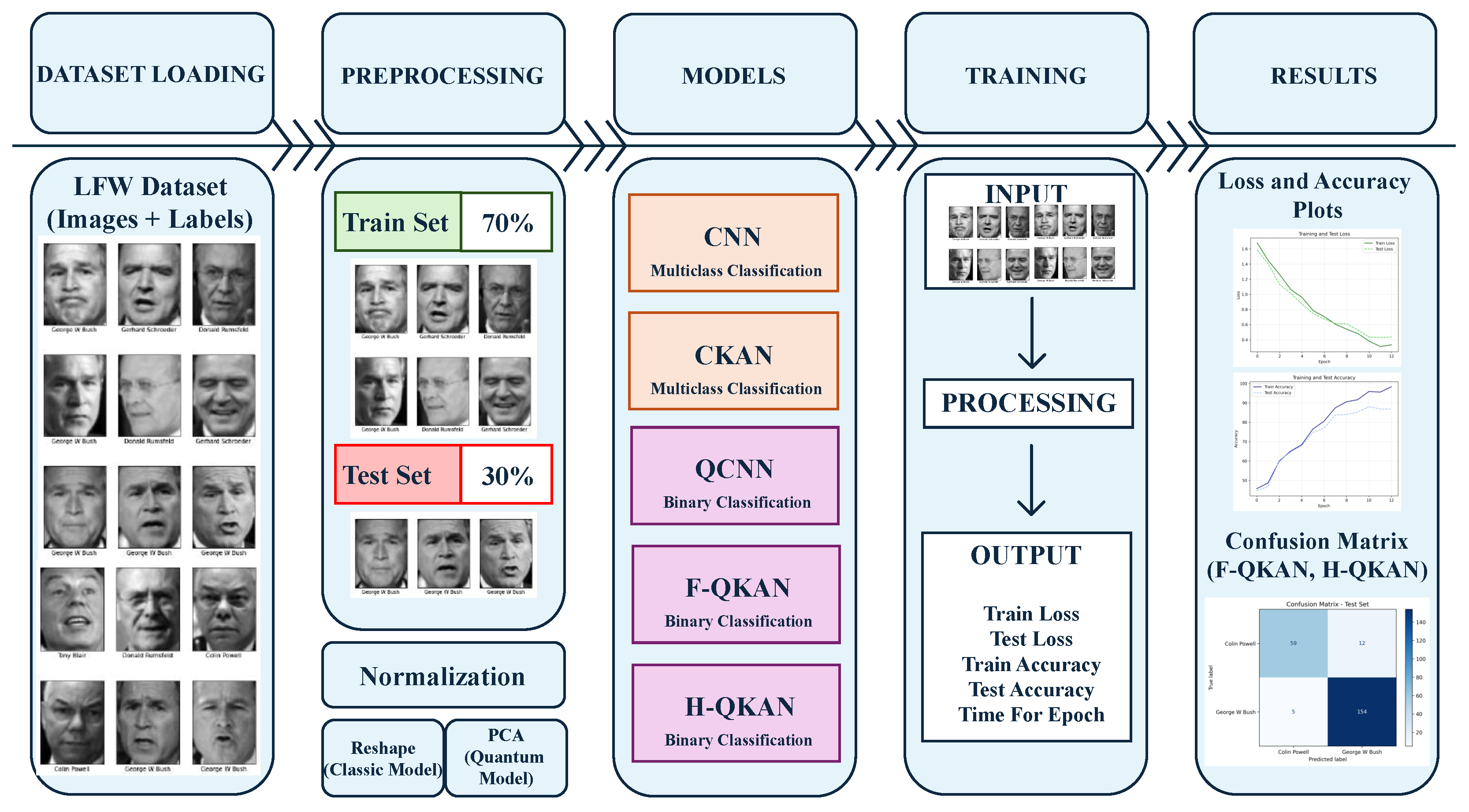
Figure 1 represents a schematic diagram summarizing the flow of the methodology.

Figure 1. Schematic diagram summarizing the flow of the methodology.

The detailed processing pipeline and the models-specific configurations are described in the following sections. All experiments were carried out in a cloud-based environment using Google Colab, ensuring a consistent and reproducible computational setup across all models.

3.2. The CNN Model

CNNs are a class of feedforward neural networks commonly used to process and make predictions on various types of data, such as text, images, video, and audio [30]. Due to their architecture, they are particularly effective in image classification and object detection, as they are able to capture complex spatial relationships within visual data by applying convolutional filters that analyze local features of the input to extract meaningful information. A CNN is typically composed of an input layer, an output layer, and several hidden layers, some of which perform convolution operations. The layers are distinguished as [31]:

• the convolutional layer that applies filters to identify local features in the data, such as edges and textures;
• the pooling layer that reduces the spatial dimensions of the input images through operations such as max pooling, which improves the robustness and generalization capabilities of the network;
• the fully connected layer that processes the features extracted from the previous layers, obtaining a final classification using an activation function; the softmax function is often used.

Building a CNN involves a preliminary data preprocessing phase and a subsequent training phase, using nonlinear activation functions, such as Rectified Linear Unit (ReLU), and optimization algorithms such as Adam. Regularization techniques, such as dropout and batch normalization, are often used to improve stability and prevent overfitting [32,33].

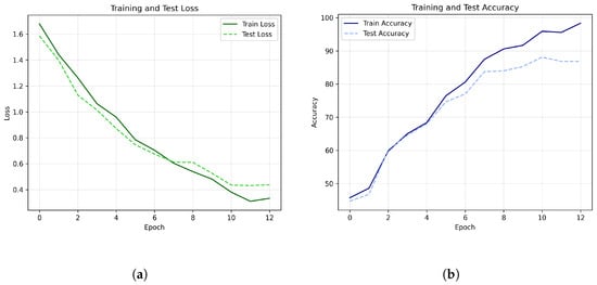
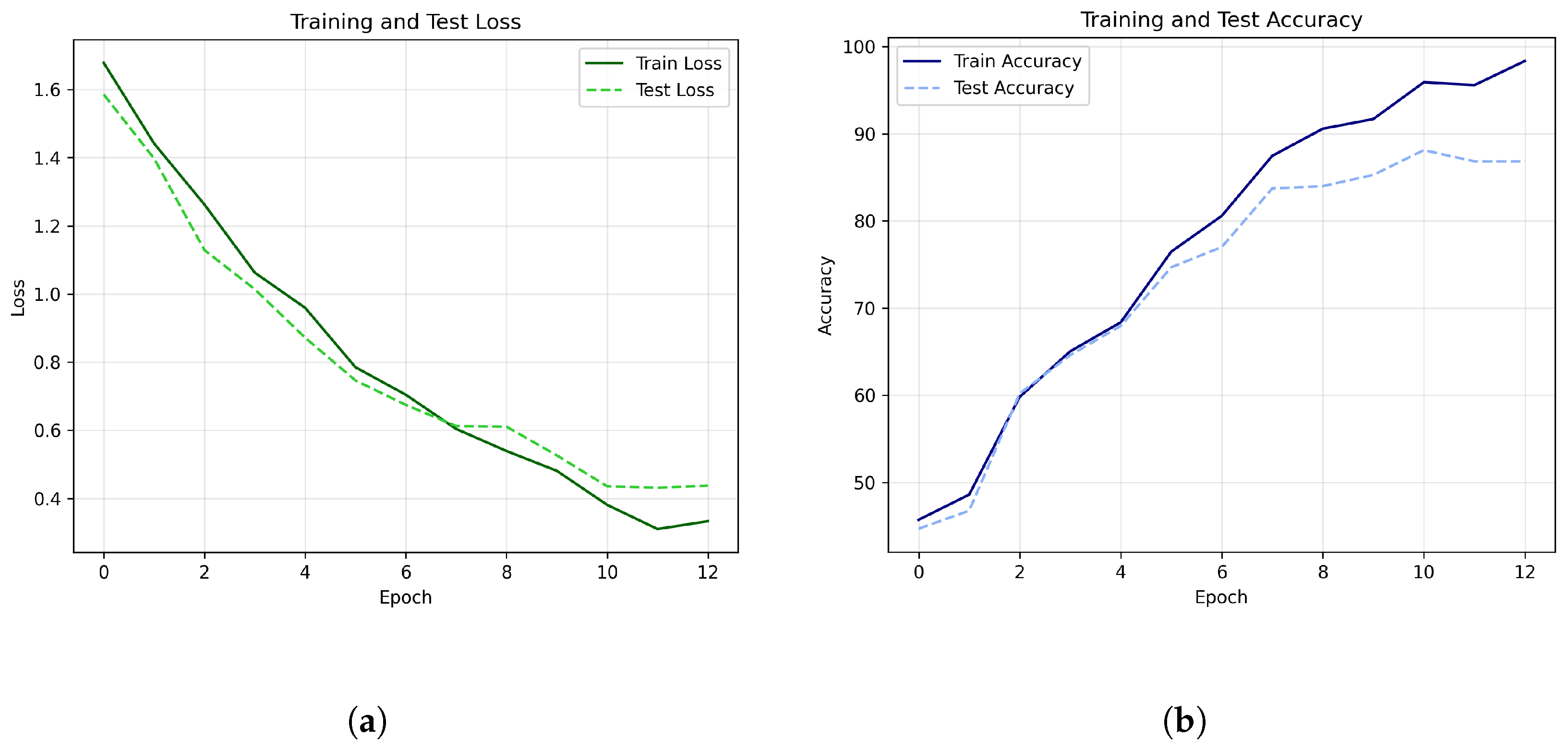
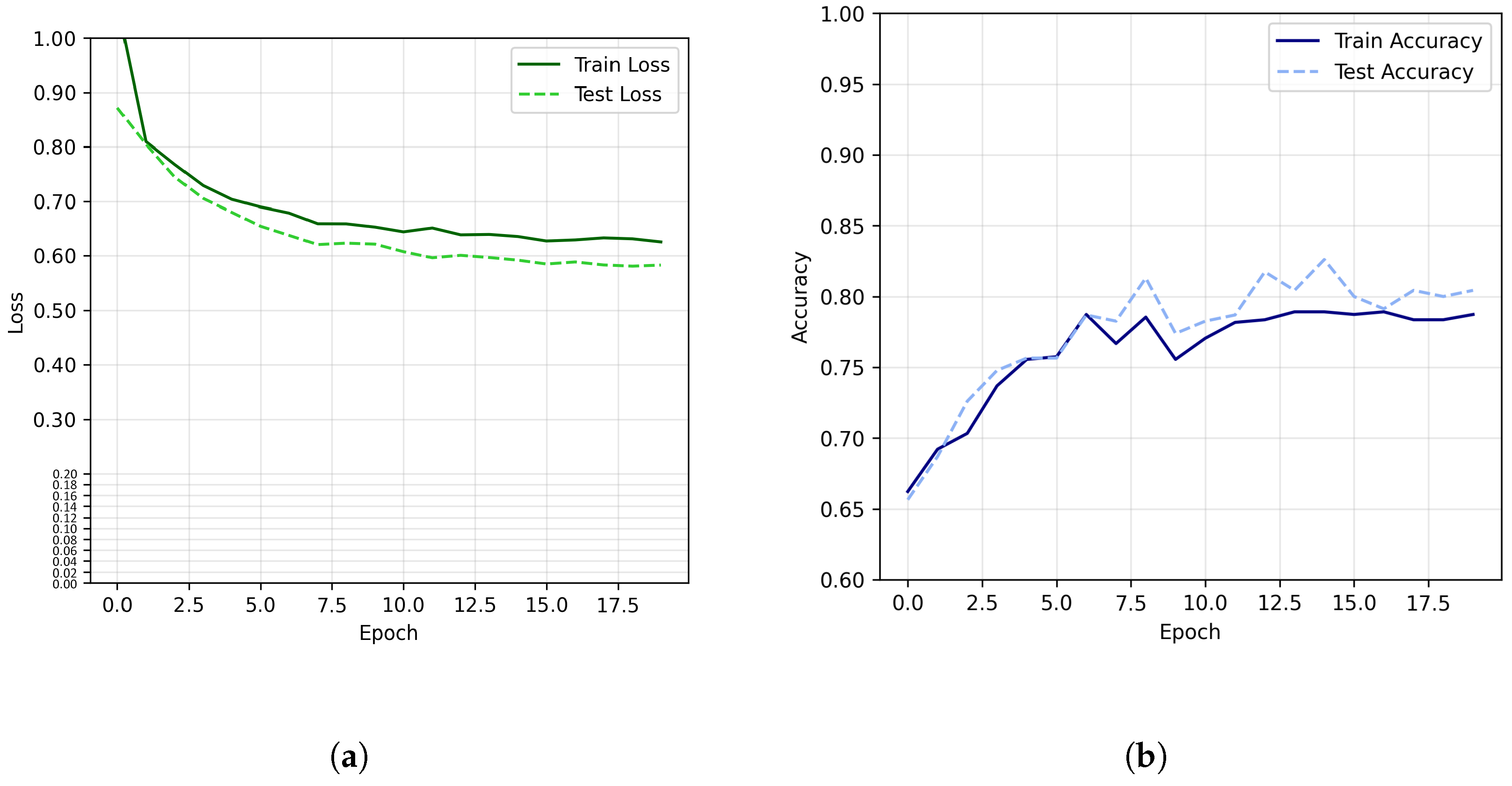
In this specific experiment, a CNN for human face recognition was implemented using the LFW dataset, limited to subjects with at least 70 images each. The images, with a resolution of 50 × 37 pixels, were normalized to even out the distribution of values and stabilize the learning process. The data were split into a training set and a test set in a 70/30 ratio, maintaining the original class distribution. The network architecture includes three convolutional blocks composed of a convolution operation followed by Batch Normalization, ReLU activation, two-dimensional MaxPooling, and Dropout with a probability of 0.25. The first block extracts 32 feature maps, the second 64, and the third 128, all with 3 × 3 kernels.The resulting features are then flattened and sent to a fully connected layer of 128 neurons, followed by a further fully connected layer that returns the membership probabilities for the seven classes in the dataset. Training was performed for up to 30 epochs (Figure 2).

Figure 2. Training metrics of CNN model. (a) Loss function. (b) Accuracy.

The Adam optimizer was used with an initial learning rate of 0.001 and a CrossEntropyLoss loss function. The batch size used was 64. The average time per epoch remained between 3.6 and 3.9 s, with negligible variations. The results show a progressive increase in performance over the course of training: the first epoch achieved a training accuracy of 45.73% and a test accuracy of 44.70%, while after just five epochs, the values rose to 68.37% and 67.96%, respectively.

The most significant increase was observed between the seventh and tenth epochs, when the test accuracy exceeded 80%, reaching 85.27% by the tenth epoch. The model achieved a maximum test accuracy of 88.11%, with a test loss of 0.435, demonstrating good generalization ability and a slight deviation from the training due to the small size of the dataset.

3.3. KAN and CKAN Network

KANs represent a promising alternative to Multilayer Perceptrons (MLPs), developed to efficiently and interpretably approximate multivariate functions. They are based on the Kolmogorov–Arnold theorem.

Theorem 1 (Kolmogorov–Arnold Representation Theorem). 

For every continuous function

$$f:{\mathbb{R}}^n\to \mathbb{R},$$

(1)

there exist univariate functions

$${\varphi }_{i,j}, g_j:\mathbb{R}\to \mathbb{R}$$

(2)

such that:

$$f(x_1,x_2,...,x_n)=\sum _{j=1}^{2n+1}{g}_j\left(\sum _{i=1}^n{\varphi }_{i,j}\left(x_i\right)\right)$$

(3)

where:

• ${\varphi }_{i,j}\left(x_i\right)$ are univariate continuous functions that transform each variable $x_i$ into a real value ${\varphi }_{i,j}\left(x_i\right)$.
• The inner sum ${\sum }_{i=1}^n{\varphi }_{i}j\left(x_i\right)$ represents a linear combination of ${\varphi }_{i}j\left(x_i\right)$ values.
• $g_j(•)$ are continuous univariate functions that map the result of the inner sum to a real value.
• The outer sum ${\sum }_{j=1}^{2n+1}{g}_j$ combines the results of $g_j$ to obtain the final value of the function $f(x_1,x_2,...,x_n).$

The theorem proves that a continuous multivariate function on a bounded domain can be written as a finite composition of continuous functions of a single variable, and on the binary addition operation [11]. Thanks to this theorem, the KANs architecture is particularly suitable for applications requiring high precision. These neural networks have a fully connected structure like MLPs, but unlike the latter, KANs applies activation functions on the edges of the network; therefore, they do not use linear weight matrices, since each weight parameter is replaced by a spline function [11].

Each function is defined by spline coefficients and a grid of control points that dynamically adapts to the data during training, thus improving the accuracy of the model [11]. Additionally, splines can also be used with activation functions, such as Sigmoid Linear Unit (SiLU), for complex relationships. An important aspect of KANs is its ability to integrate symbolic components that allow it to explicitly represent already known mathematical functions, such as logarithms or powers [11]. In this way, KANs offers a level of interpretability that other deep learning models struggle to achieve, making it particularly suitable for contexts where transparency and model understanding are key requirements [11].

The learning process in KANs uses automatic optimization by differentiation, an approach that allows for flexible combinations of different objectives: starting from a Mean Squared Error (MSE), L1 regularization elements and entropy-based penalties are added, with the aim of pushing the network to generate simpler and more readable models [11]. KANs can be trained with common optimizers like Adam, but it also supports more sophisticated methods, such as Limited-memory BFGS (LBFGS), which are particularly effective when working with limited datasets [11].

The Pykan library (The library is available on GitHub at https://github.com/KindXiaoming/pykan, accessed on 1 November 2025) is a framework designed for implementing and training KANs [11]. Experiments were conducted using CKAN networks, an architecture that incorporates KANs, as they have demonstrated superior performance in image classification tasks.

The implemented model is a CKAN, a fusion of the CNNs and KANs networks: convolutional layers extract spatial features from the input images, while KAN layers replace the traditional fully connected layers with spline functions [12]. This hybrid architecture achieves an optimal balance between computational efficiency and representation power, making it ideal for advanced computer vision applications [12]. The experiment was designed to classify images from the LFW dataset. The images were scaled and normalized to include the channel, and then split them into training (70%) and testing (30%) sets. The data was then converted into tensors and loaded using DataLoader.

The network features two convolutional layers: the first consists of a 2-dimensional convolution with 1 input channel and 32 filters with a 3 × 3 kernel and 1 padding, followed by SELU activation and a max-pooling operation with a 2 × 2 kernel that reduces the spatial dimensions by half; the second consists of a convolution with 32 input channels and 64 filters, a 3 × 3 kernel and 1 padding, followed by SELU and 2 × 2 max-pooling, which further reduces the spatial dimensions to a quarter of the original. The convolutional output is then transformed into a vector of dimension 64 × h/4 × w/4 and passed to a KAN layer, which receives the transformed vector as input and produces 32 units. The second KAN layer maps these 32 units to the classes in the dataset, generating the final logits for classification. The output dimension after pooling is dynamically calculated to ensure compatibility with subsequent layers. This combination of CNN and KAN leverages the feature extraction capabilities of CNNs along with the flexibility of spline-based transformations, making the model more interpretable and suitable for analyzing structured and complex data.

The CKAN architecture is particularly suited to handling compressed input data, such as the principal components obtained from a Principal Component Analysis (PCA) transformation. By combining a linear base transformation with flexible spline-based nonlinear mappings, each KAN layer can adaptively model variations in the reduced feature space. This allows the network to capture complex dependencies even in low-dimensional representations, providing robust and interpretable features for subsequent processing or classification.

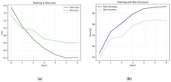
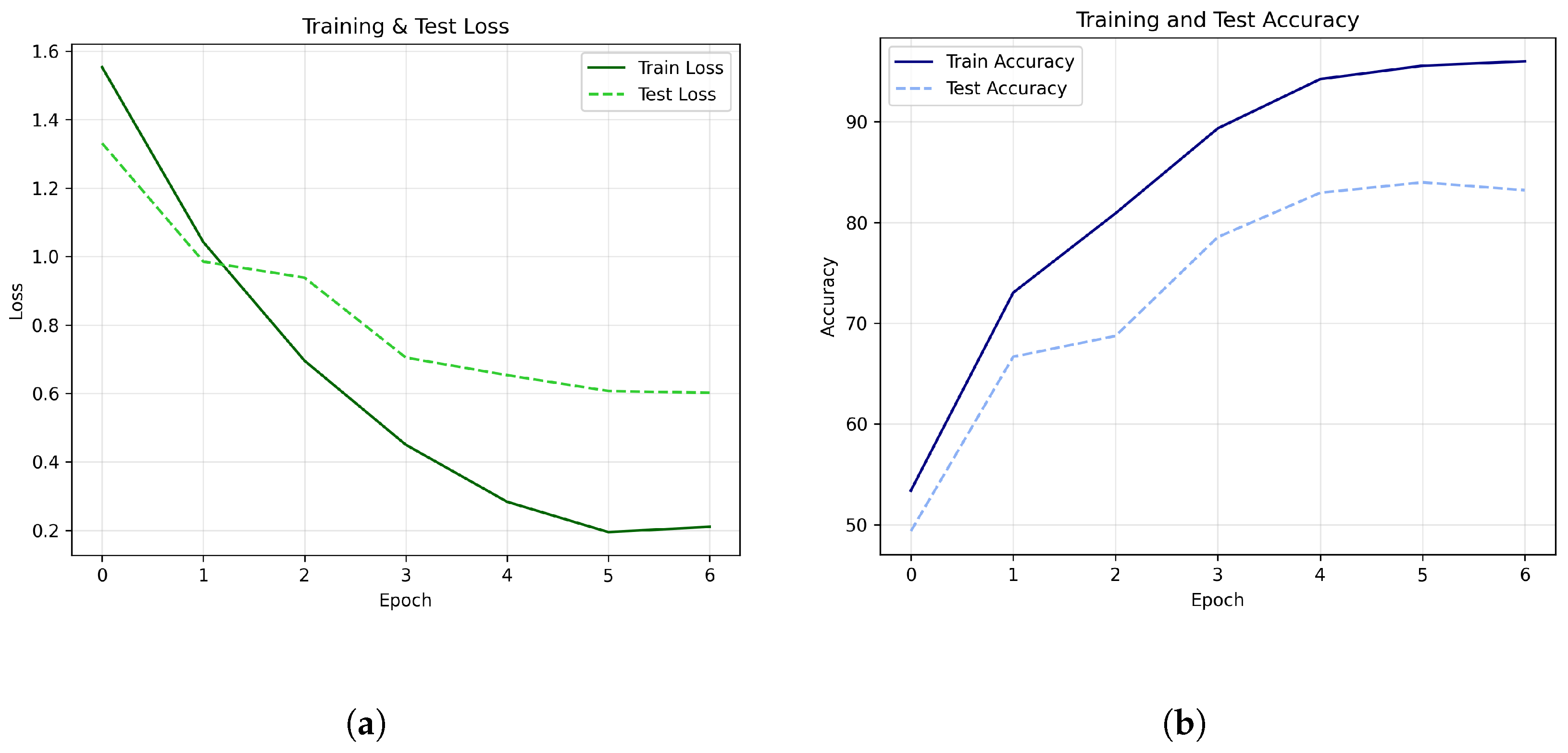
The model uses CrossEntropyLoss as the loss function and the Adam optimizer with a learning rate of 0.001. Training was conducted for 30 epochs, during which the training and test losses and accuracies were monitored, and the graphs were saved. In particular, the training results (Figure 3) show that the CKAN model exhibits a progressive reduction in loss on both the training and test sets, accompanied by an increase in accuracy for both the training and test sets.

Figure 3. Training metrics of CKAN model. (a) Loss function. (b) Accuracy.

The training loss decreases steadily from the first epochs until stabilizing at low values, while the test loss follows a similar trend, indicating an improvement in the model’s overall performance. Training accuracy increases rapidly, while test accuracy grows steadily, stabilizing at lower values than training (the maximum test accuracy achieved is 83.98%). The time trend per epoch shows consistent and relatively stable execution times (approximately 14 s), with training stopping when the training accuracy criterion is reached. Overall, the data shows model convergence, with decreasing losses and increasing accuracies.

3.4. Reduction of Dimensionality and Quantum Constraints

Following the convergence observed in classical and hybrid models, quantum architectures introduce additional constraints related to feature dimensionality, qubit availability, and circuit depth. In this context, dimensionality reduction via PCA enables the construction of more tractable quantum circuits, improving feasibility and robustness to noise at the cost of discarding part of the original information. Conversely, retaining a larger number of principal components preserves richer feature representations but proportionally increases qubit requirements and circuit depth, amplifying entanglement operations and cumulative noise, as well as simulation time under NISQ conditions.

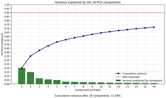
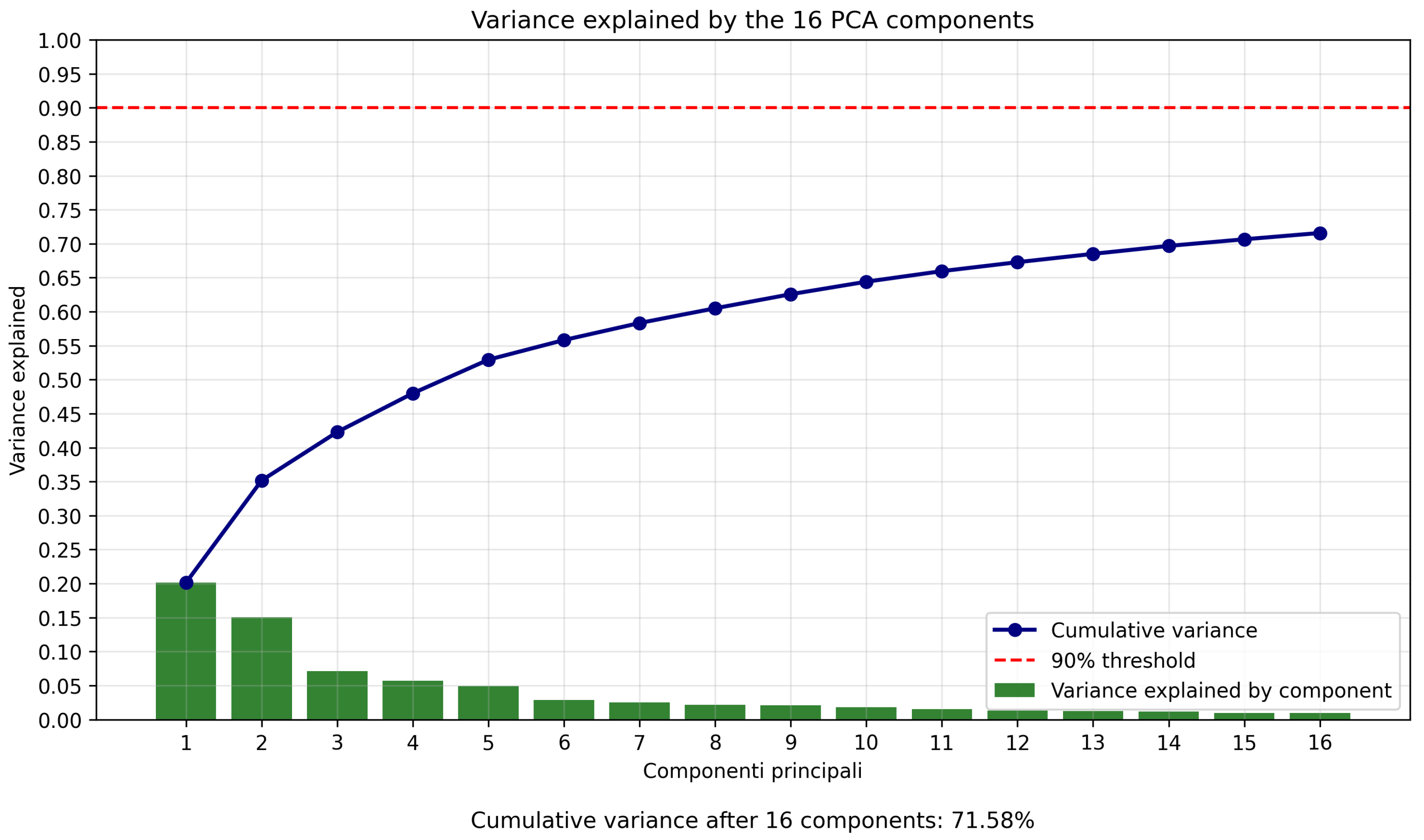
For the experiments in this work, reducing the input to 16 principal components represented a pragmatic compromise: it preserves approximately 72% of the variance while remaining compatible with few-qubit circuits, aligned with current NISQ hardware constraints. This setting allows us to evaluate quantum and hybrid models within current hardware feasibility, while still maintaining a representational capacity sufficient for comparison across architectures.

3.5. Quantum Machine Learning

This part describes the approach used to design and evaluate the QCNN architecture for image classification. The process consists of several essential steps, including data preprocessing, mapping classical data into quantum states, constructing the quantum convolutional layers, and incorporating realistic noise models to reflect hardware imperfections. These experiments have been conducted using PennyLane v.0.41 to simulate quantum circuits, while Scikit-learn is used for the preparation and handling of classical data. This methodology aims to explore both the strengths and current limitations of QCNNs in ideal conditions and under the influence of quantum noise, following core principles of quantum machine learning as discussed in prior literature [19].

As described in Section 3.1, the LFW dataset [4] is adopted for the experiments. To ensure a balanced and computationally feasible task, the focus is placed on a binary classification problem distinguishing between the identities “Colin Powell” and “George W. Bush”, selecting only those classes with at least 200 images. All images are converted to greyscale and normalized to the $[0, 1]$ range before quantum encoding.

To make everything homogeneous, the experiments were redone with modifications that did not affect the network structure.

To adapt the dataset to the constraints of current quantum hardware, the dimensionality is reduced by using PCA applied only to the training data after splitting the dataset (70% training and 30% test) to avoid data leakage.

This transformation projects the data onto a lower-dimensional subspace while preserving the most significant features. Mathematically, this is expressed as in Equation (4),

$$X_{\mathrm{PCA}}=X·W_{\mathrm{PCA}},$$

(4)

where X denotes the original data matrix and $W_{\mathrm{PCA}}$ contains the eigenvectors corresponding to the largest eigenvalues of the covariance matrix of X. For quantum encoding, angle embedding is using to map classical data vectors $x\in {\mathbb{R}}^d$ (after PCA) into quantum states via rotations around the X-axis, as in Equation (5),

$$|\psi ⟩=\prod _{i=1}^d{R}_X\left(x_i\right)|0⟩,$$

(5)

where $R_X\left(x_i\right)$ is a single-qubit rotation gate parameterized by the i-th feature. This approach ensures that the input data is efficiently represented in the quantum Hilbert space.

The QCNN architecture is built from repeated layers of parameterized gates and entangling operations. Each layer consists of a sequence of single-qubit rotations and Controlled NOT (CNOT) gates, described by the unitary transformation:

$$\begin{array}{cc}\hfill U_{\mathrm{layer}}\left(\theta \right)=& {\displaystyle \prod _{i=1}^d}\mathrm{CNOT}(i,(i+1) \mathrm{mod} d)·\hfill \\ & {\displaystyle \prod _{i=1}^d}{R}_Z\left({\theta }_{i,1}\right)R_Y\left({\theta }_{i,2}\right)R_Z\left({\theta }_{i,3}\right),\hfill \end{array}$$

(6)

where ${\theta }_{i,j}$ are trainable parameters. To improve generalization and prevent overfitting, a dropout is integrated into the quantum circuit by applying depolarizing channels after each layer. The effect of dropout on a quantum state $\rho$ is modelled as in Equation (7).

$${\mathcal{E}}_{\mathrm{dropout}}\left(\rho \right)=(1-p)\rho +{\displaystyle \frac{p}{2^n}}I,$$

(7)

where p is the dropout probability, n is the number of qubits, and I is the identity matrix.

To simulate real-world hardware imperfections, depolarizing and phase-slamming noise channels were also included after each layer. These are given by Equations (8) and (9),

$${\mathcal{E}}_{\mathrm{depolarizing}}\left(\rho \right)=(1-p)\rho +{\displaystyle \frac{p}{3}}(X\rho X+Y\rho Y+Z\rho Z),$$

(8)

$${\mathcal{E}}_{\mathrm{phase} \mathrm{damping}}\left(\rho \right)=(1-p)\rho +pZ\rho Z,$$

(9)

which model decoherence and environmental effects in noisy intermediate-scale quantum devices. A cost function combining MSE with Norm L2 (L2) regularization is adopted as in Equation (10),

$$\mathcal{L}\left(\theta \right)={\displaystyle \frac{1}{N}}\sum _{i=1}^N{(y_i-f(x_i;\theta ))}^2+\lambda {\parallel \theta \parallel }_2^2,$$

(10)

where $y_i$ is the true label, $f(x_i;\theta )$ is the model prediction, and $\lambda$ is the regularization coefficient. Optimization is performed using the Adam algorithm with a decaying learning rate, defined at epoch t by (11),

$${\eta }_t={\displaystyle \frac{{\eta }_0}{\sqrt{t}+ϵ}},$$

(11)

where ${\eta }_0$ is the initial learning rate and $ϵ$ is a small constant for numerical stability.

This methodology constitutes a complete pipeline for the development and evaluation of QCNNs in both ideal and noisy environments. The inclusion of noise models and dropout mechanisms provides insights into the feasibility and robustness of deploying quantum models on real hardware.

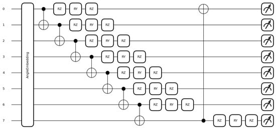
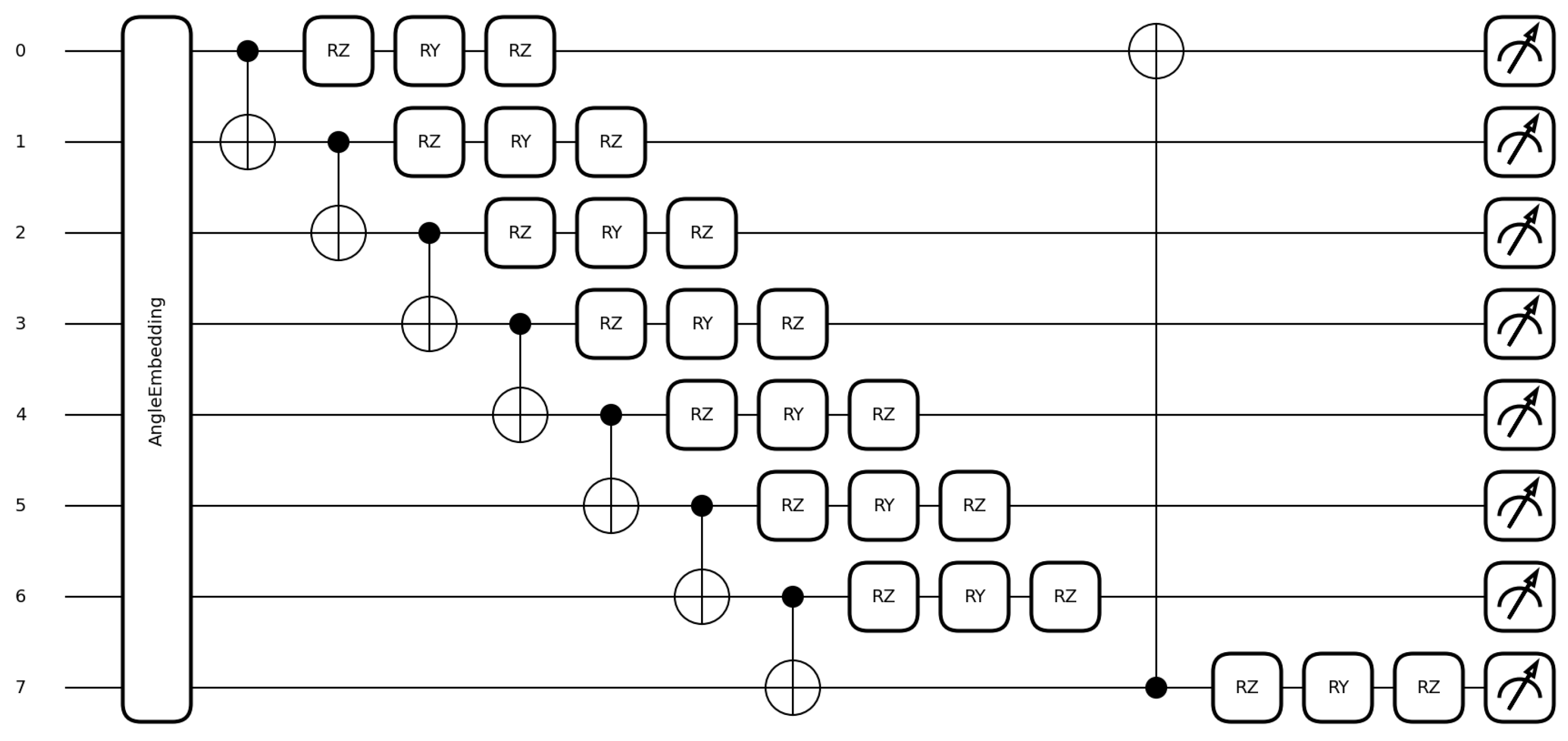
Figure 4 shows the structure of a single QCNN layer, from angle embedding through trainable gates and noise injection.

Figure 4. Quantum circuit representation of a single QCNN layer.

Starting from the described methodology, the experiments aim to evaluate the capabilities of QCNN in ideal conditions and in contexts affected by quantum noise, simulating the use on real hardware.

The following is an experiment designed to evaluate the performance of QCNN in noise-free and noisy conditions, consistent with the limitations of current quantum hardware.

Continuing from the methodology described above, the LFW dataset was preprocessed using Scikit-learn by normalizing pixel values and flattening images into feature vectors. The data was split into training (70%) and testing (30%) sets, maintaining class balance. Only after this preprocessing step was PCA applied, reducing the data to eight principal components in order to meet the computational constraints of the available hardware and enable efficient quantum embedding.

QCNNs were implemented in PennyLane using ten layers, each composed of parameterized single-qubit rotations and CNOT entanglement. Angle embedding mapped each 8-dimensional input to quantum states, and Pauli-Z expectation values were used for output measurement.

Training used the Adam optimizer with a learning rate of 0.05. The cost function combined MSE and L2 regularization. Simulations were run for both 5 and 10 epochs using the default.qubit (ideal) and default.mixed (noisy) backends. The noise model included depolarizing (0.01) and phase damping (0.02) channels.

Each noiseless layer used 40 gates, totaling 240 parameters. In the noisy setting, two additional noise operations per qubit increased the gate count to 72 per layer. The full implementation of all models discussed in this work, including the QCNN, CNN, and CKAN architectures, is available on GitHub (https://github.com/fabionpl/ICCSA25, accessed on 1 November 2025).

The network was trained using both 5 and 10 epochs to evaluate its convergence behavior. In both cases, the model showed a rapid improvement in performance in the first few epochs, followed by a progressive stabilization of loss and accuracy values.

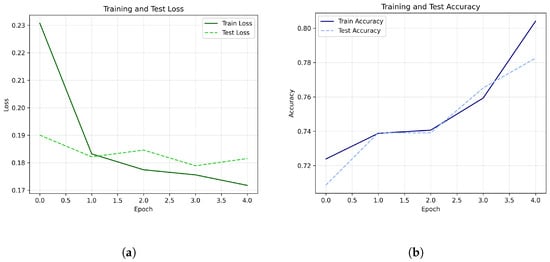
With 5 epochs (Figure 5), the network already achieved solid results, with a test accuracy of approximately 78% and a stable learning curve, free of overfitting.

Figure 5. Training metrics of noise-free QCNN model (5 epochs). (a) Loss function. (b) Accuracy.

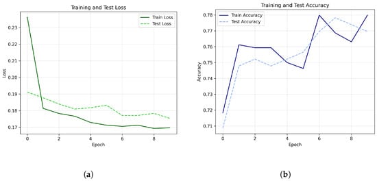
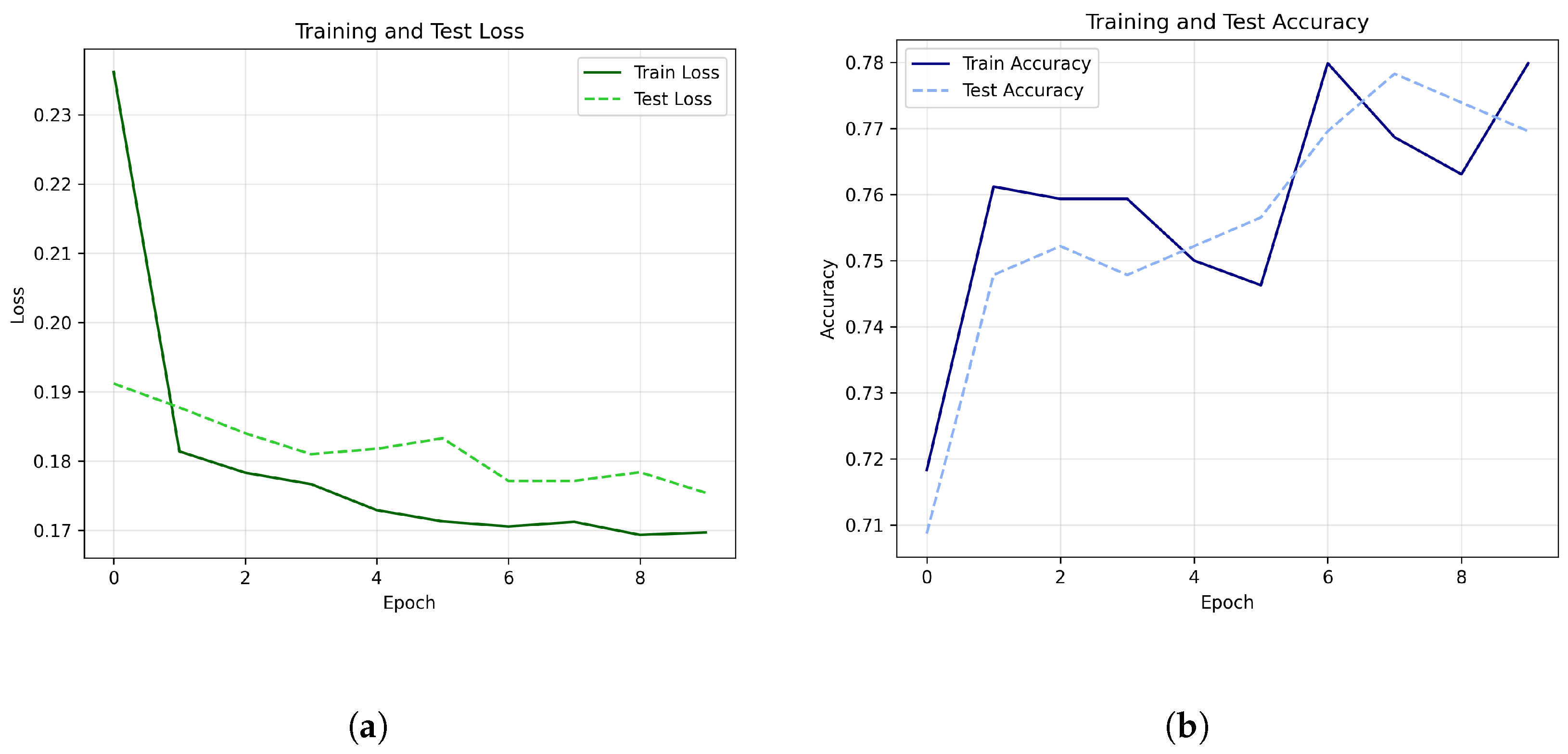
Extending the training to 10 epochs, (Figure 6), resulted in more regular convergence and greater consistency between training and testing results, confirming the model’s good generalization ability.

Figure 6. Training metrics of noise-free QCNN model (10 epochs). (a) Loss function. (b) Accuracy.

The best performance was observed at the eighth epoch, where the test accuracy exceeded 77%; in subsequent epochs, the metrics remained stable, demonstrating the robustness and reliability of the training process.

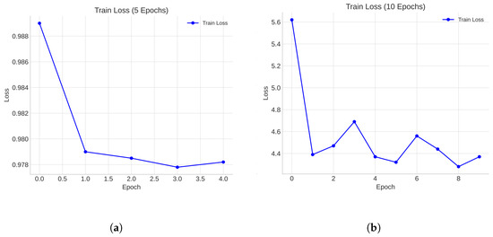
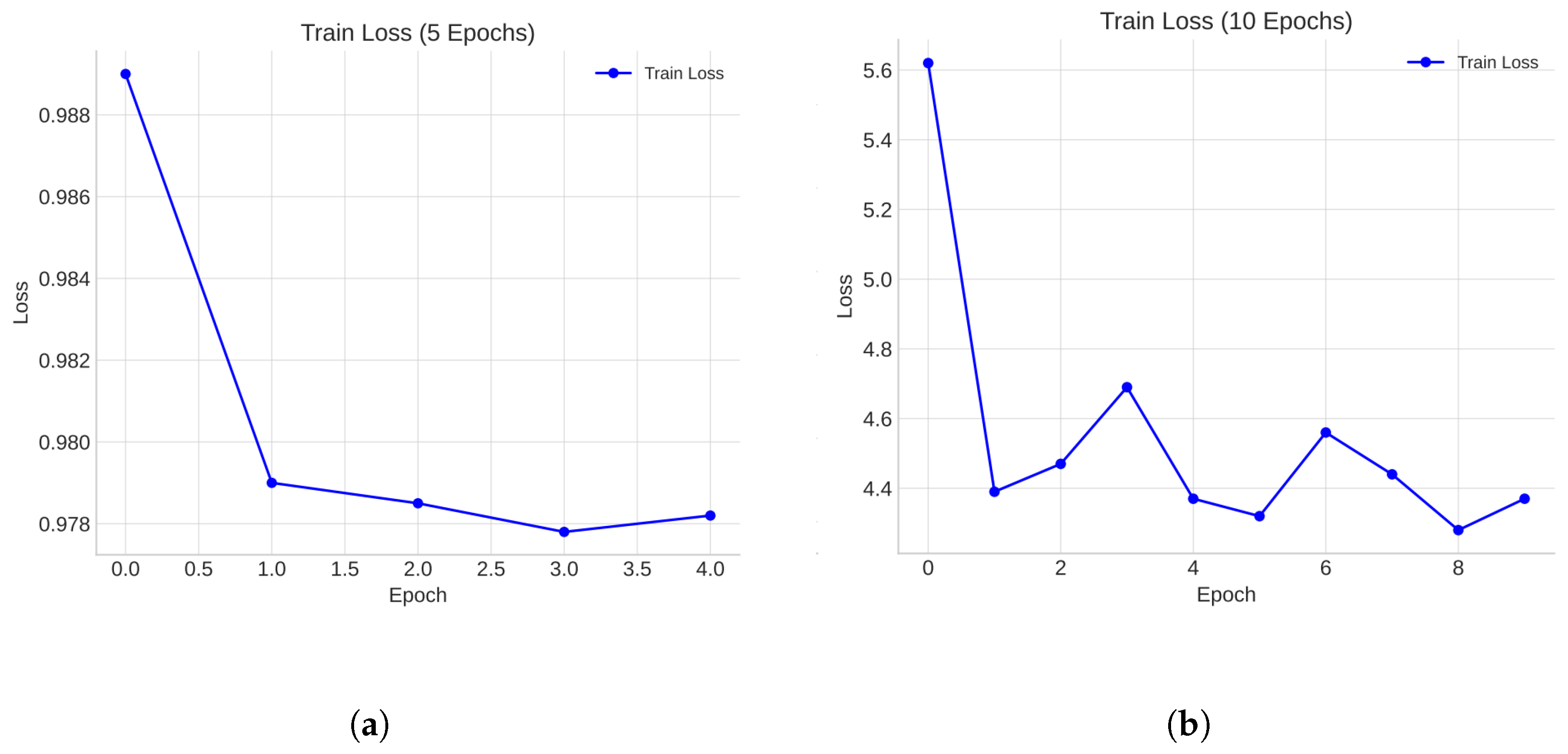
In the noisy model, the loss function shows an initial phase of model adaptation, followed by a progressive stabilization trend. In the early epochs (Figure 7), the network shows a reduction in loss, a sign of an effective learning process despite the presence of noise in the quantum system.

Figure 7. Noisy QCNN: training loss after 5 epochs (a) and training loss after 10 epochs (b).

As training progresses, a less regular evolution of the loss function is observed, with oscillations that reflect the complexity of optimization dynamics in noisy quantum environments.

3.6. Integration Models

As in previous sections, experiments were conducted on the LFW by implementing two new networks: a fully quantum model (F-QKAN) and a hybrid model (H-QKAN), combining the best of classical and quantum machine learning.

Quantum circuits were simulated using the Pennylane library, while classical data preparation and management were performed with Scikit-learn. For the Hybrid Model only, the Pykan library was used to build the KANs part of the network.

3.6.1. F-QKAN

The first goal was to build a fully quantum KAN. This work drew inspiration from recent theories, particularly the Kolmogorov–Arnold theorem and the work of Ivashkov et al. [15] and Daskin [16]. Although the formulas were not replicated exactly, the fundamental principles were adopted: decomposing complex functions into simpler (univariate) operations and adapting them to a variational circuit.

In the quantum context, a KAN can be thought of as a network in which the fundamental operations are performed by unitary transformations on the individual qubits (which act like the univariate operations of the KAN), then combined via bounded entanglement.

For the experiment, again, the LFW was used, selecting the two classes with at least 200 images per subject. The images were normalized and transformed into vectors, and PCA was applied to reduce noise and focus on the essential information, lowering the dimensionality to 16 principal components explaining approximately 72% (Figure 8) of the variance while preserving most of the information.

Figure 8. Variance explained by the 16 principal components of PCA.

To encode the data in the quantum circuit, the values were scaled to a range from 0 to $\pi$. It is important to note that PCA was computed only on the training data to avoid data leakage. The model is based on an 8-qubit variational circuit. Each qubit encodes one of the 8 main features extracted from the PCA.

This circuit is composed of a sequence of 10 Quantum Kolmogorov–Arnold layers (QKA-layers). Each layer is designed to replicate the conceptual functioning of a classical KAN layer [15]. In this context, the KAN layer is not implemented via classical spline functions but as a block of unitary transformations designed to simulate combinations of univariate and multivariate functions according to the Kolmogorov–Arnold principle: a series of parameterized local rotations is initially applied ($R_X$, $R_Y$, $R_Z$).

These rotations rapresent the quantum equivalent of the spline functions learned in classical KANs. They allow each qubit to process its own portion of the input independently. Local interactions are then introduced through IsingXX operators, which combine the previous univariate transformations. Finally, CNOT operations connect distant qubits, modeling more complex nonlinear relationships and global dependencies [15,16].

In summary, quantum rotations replace univariate splines, while entanglement operations represent the functional combinations typical of classical KANs. The output of the circuit, providing the binary prediction, is measured using the expectation value of the Pauli operator $Z_0$.

Thus, each layer includes local rotations on the qubits ($R_X$, $R_Y$, $R_Z$) and both local (IsingXX) and non-local (CNOT) two-qubit interactions, for a total of approximately 34 gates per layer. The execution was performed using PennyLane’s default.qubit simulator, calculating the expectation values directly without the need for sampling, i.e., without using a finite number of shots. This architecture is particularly suitable for current quantum devices (NISQ) because, while being expressive, it has a small number of parameters and a controlled depth [17].

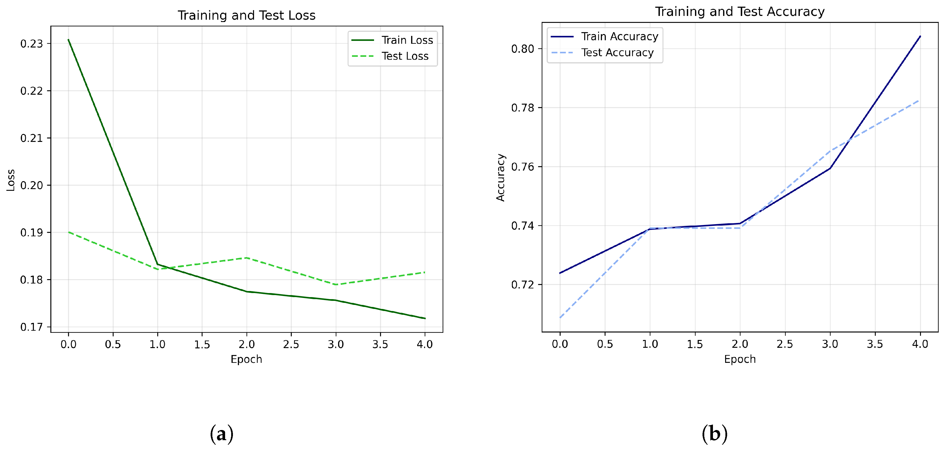
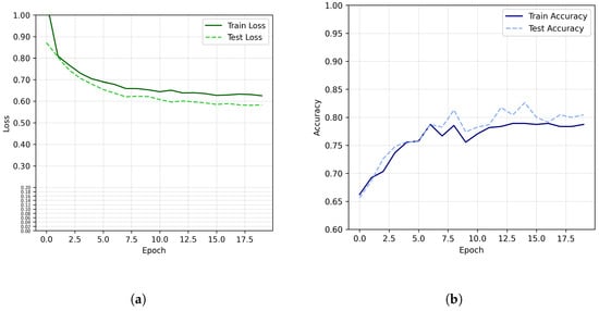
Training was conducted for a maximum of 30 epochs (Figure 9) with a batch size of 8.

Figure 9. Training metrics of F-QKAN model. (a) Loss function. (b) Accuracy.

During the first epochs, the model showed a steady improvement in both loss and accuracy, reaching a plateau after approximately the tenth epoch.

The maximum accuracy on the test (82.61%) was achieved at the 15th epoch (Table 1), while since 20th epoch, no improvements have been recorded. The average time per epoch was approximately 373 s, in line with the computational complexity of the 10-layer quantum circuit simulated on a CPU.

Table 1. Training and testing metrics performance across epochs of the F-QKAN model.

Epoch	Train Loss	Test Loss	Train Acc	Test Acc	Average Time (s)
1	1.0620	0.8717	0.6523	0.6565	382.1
5	0.7036	0.6799	0.7556	0.7565	377.0
9	0.6588	0.6232	0.7854	0.8130	368.1
15	0.6354	0.5917	0.7892	0.8261	373.8
20	0.6254	0.5826	0.7873	0.8043	363.8

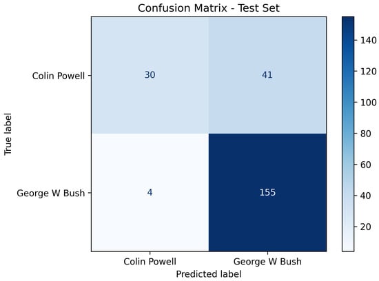
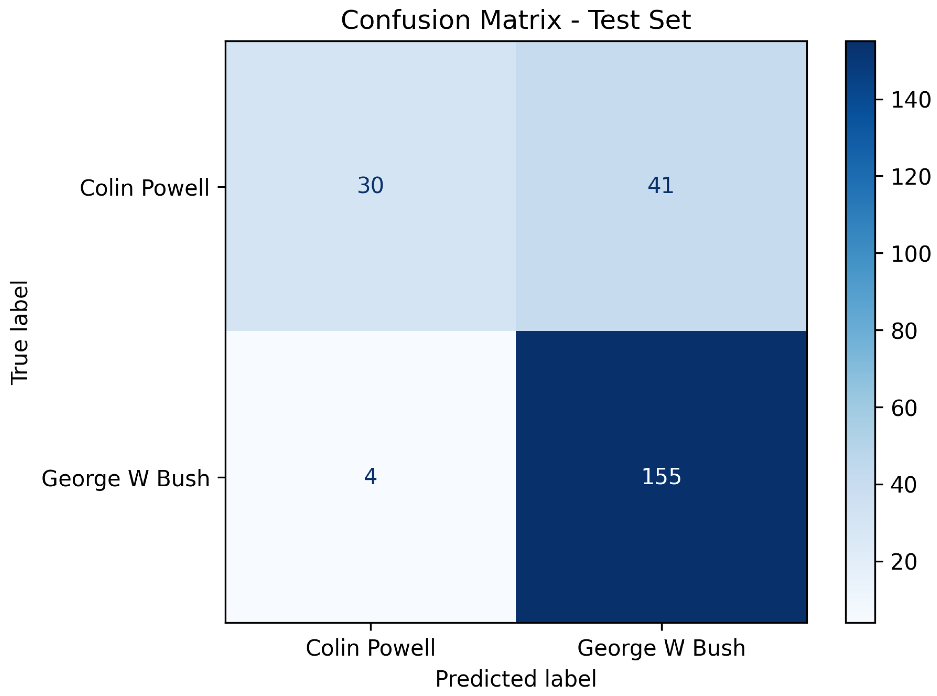
The confusion matrix (Figure 10) calculated on the test set shows 155 correct and 41 incorrect classifications for the “George W. Bush” class and 30 correct and 4 incorrect for the “Colin Powell” class, indicating good overall discriminative ability, with a slight asymmetry due to the different number of classes.

Figure 10. Confusion Matrix of F-QKAN model.

3.6.2. H-QKAN

The hybrid model is an approach that aims to combine the power of classical representation with the ability of quantum circuits to make complex decisions. A classical KAN was used as an interpretable feature extractor, implemented through the pykan library, and a Variational Quantum Circuit (VQC) as the final classification layer, implemented through the Pennylane library.

This configuration aligns with recent work by Kundu et al. [17] and Wakaura et al. [18].

Unlike Section 3.2, a binary classification was performed by considering only the first two classes of images with at least 200 images per person. These were normalized and flattened into 1D vectors. To reduce the dimensionality of the images, PCA was applied only on the train data (to avoid data leakage) keeping 16 principal components (Figure 8) that explain most of the information (72%). Subsequently, all features were mapped to the range [0, 1].

KAN was crucial because it replaces the linear connections of traditional neural networks (MLPs) with parametric univariate spline functions that are learned during training. This enables it to dynamically adapt its no-linearity. As shown in Kundu et al. [17], this structure is important because it greatly reduces the number of parameters and makes the learning process more interpretable and stable. Furthermore, the spline-based nature of the activations allows for better management of noise and data complexity, a feature particularly useful in the quantum context and in applications on NISQ hardware [17].

The implemented KAN model was defined with a three-layer structure ([16, 32, 8]). The network is trained in a completely classical manner, using a mean squared error loss function optimized with an adaptive gradient descent algorithm. The goal of the KAN network is to learn a compact representation of the images, and at the end of training, the output vector is used as the input feature for the quantum classifier built according to the Variational Quantum Algorithms (VQA) paradigm [18]. The extracted features are encoded in the initial state of the quantum circuit through one-dimensional rotations ($R_Y$) applied to each qubit. Subsequently, generic parameterized rotations around the X, Y, and Z axes were defined on each qubit, along with a chain of CNOT operations to introduce entanglement between adjacent qubits. The final measurement of the Pauli operator ($Z_0$) provides the classifier’s prediction.

The entire process is optimized using the Adam algorithm, which calculates the distance between the quantum expected value and the encoded class label in the range [−1, 1], allowing for an iterative update of the quantum parameters through a classical–quantum optimization cycle. The employed VQC can be considered a simplified version of a Quantum Neural Network (QNN) [17,18], but with a reduced number of parameters and an interpretable structure, consistent with the adaptive approach introduced in Adaptive VQKAN [18].

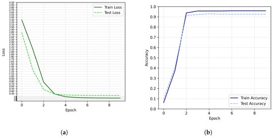
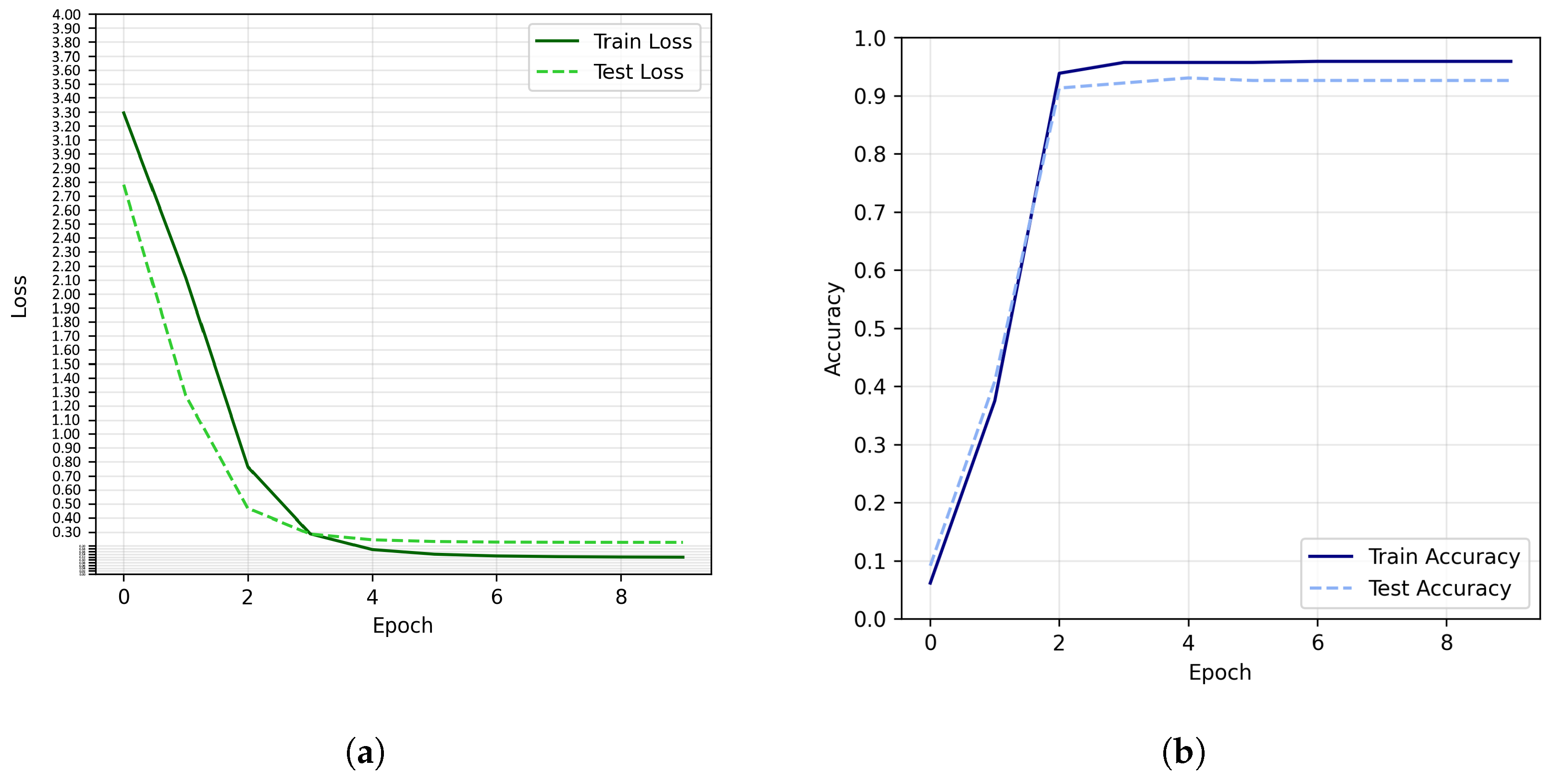
The H-QKAN demonstrated high stability and rapid convergence during the training phase. Training was performed for up to 30 epochs (Figure 11) using the MSE cost function with L2 regularization and the Adam optimizer, with a learning rate of 0.005.

Figure 11. Training metrics of H-QKAN model. (a) Loss function. (b) Accuracy.

Accuracy and loss metrics were monitored on both the training and test sets. A clear and progressive improvement in performance was observed during training (Figure 11). The training loss showed a significant decrease from 3.29 to approximately 0.12, while the test loss followed a similar trend, stabilizing around 0.23 starting from the eighth epoch. Consequently, training accuracy progressively increased to 95.90%, with test accuracy stabilizing at 92.61% in the final epochs, reaching a maximum value of 93.04% at the fifth epoch, indicating excellent generalization ability and robust model convergence.

Training has stabilized since the 10th epoch. The average time per epoch was approximately 40 s, highlighting the computational efficiency of the implemented architecture even in the presence of a simulated quantum circuit.

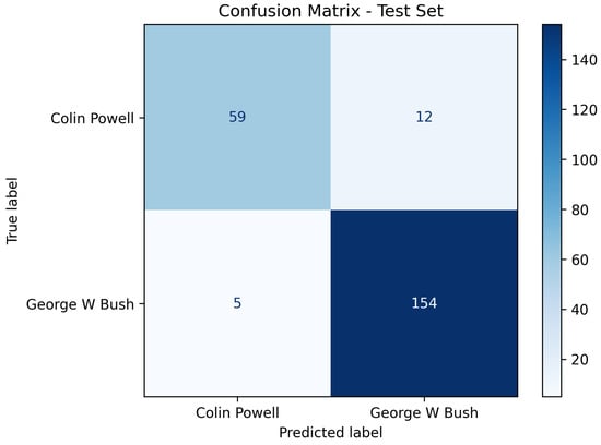
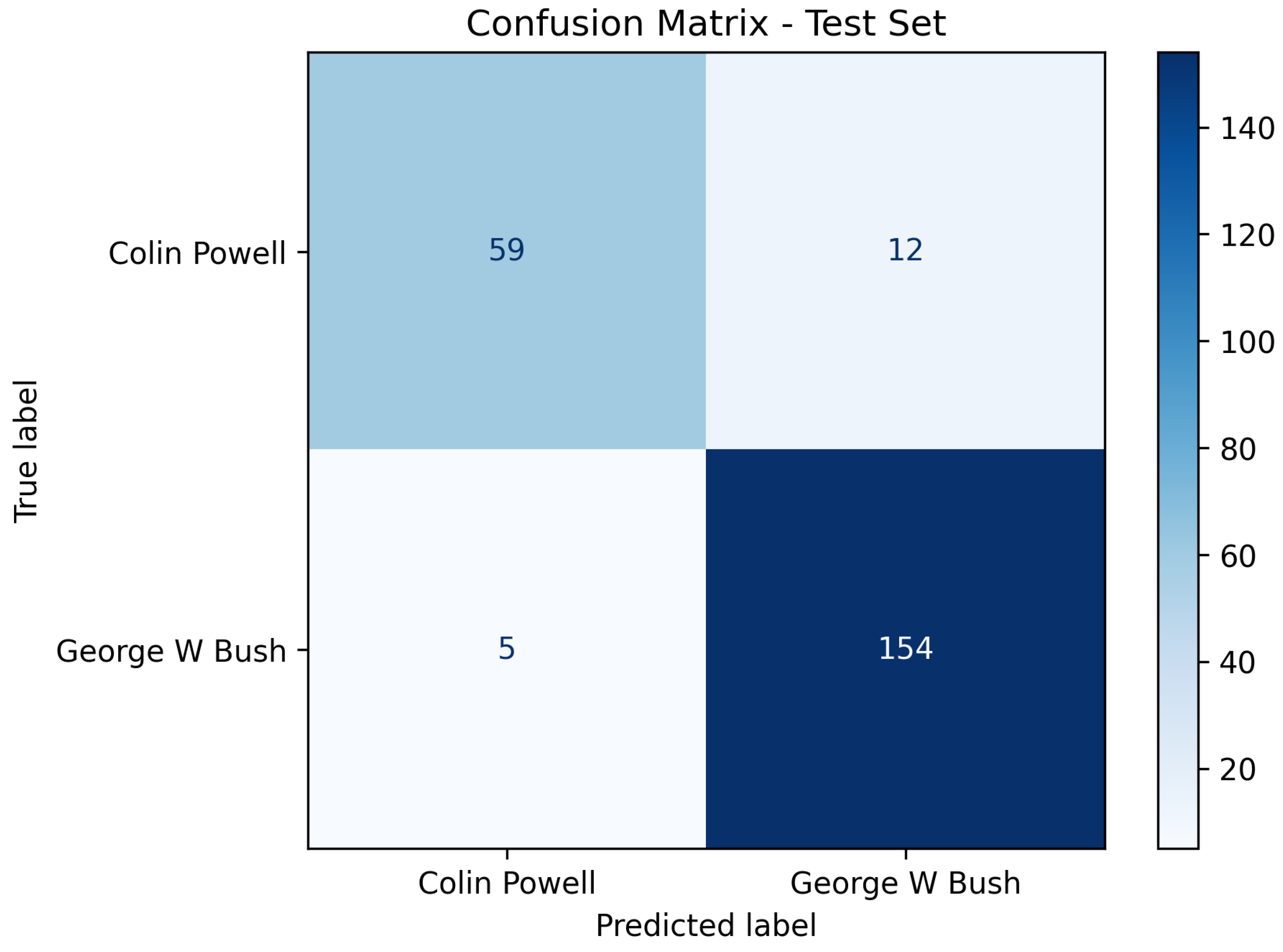
The confusion matrix (Figure 12) on the test set shows high accuracy for both classes considered.

Figure 12. Confusion matrix of H-QKAN model.

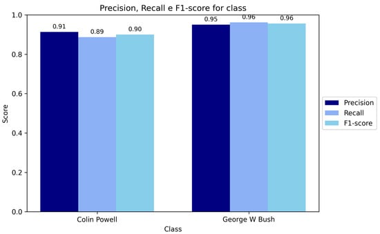
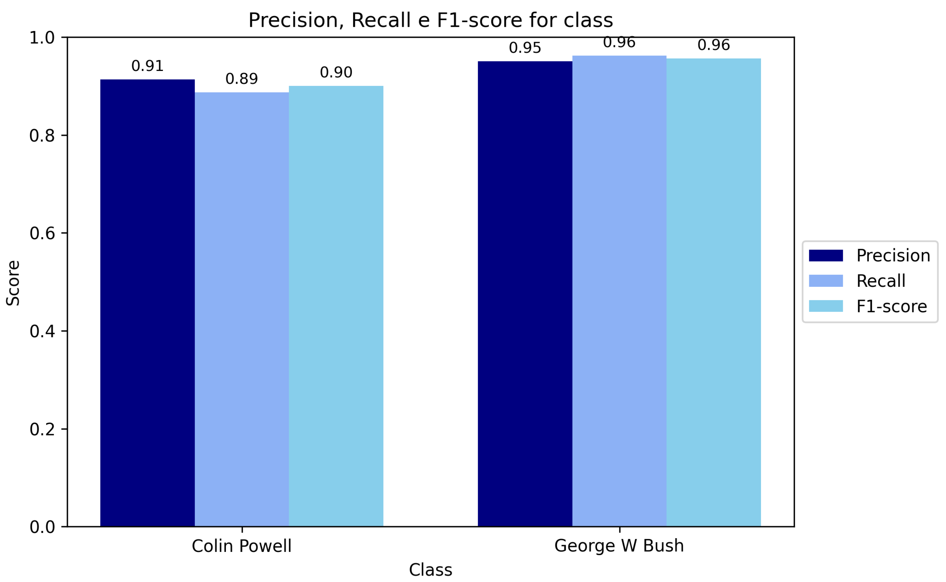
Specifically, the model correctly classified most of the samples belonging to “George W. Bush” (154 correct out of 159) and “Colin Powell” (59 correct out of 71), showing a low incidence of false positives and false negatives, confirming the overall effectiveness of the adopted hybrid approach. As a complementary analysis, precision, recall, and F1-score were computed for each class. These metrics offer additional insight into the classification behavior and are reported in Figure 13.

Figure 13. Class-wise precision, recall, and F1-score of the hybrid model.

3.6.3. Explainability

Explainability, or interpretability, is recognized as a key strength of KANs compared to traditional MLPs [16].

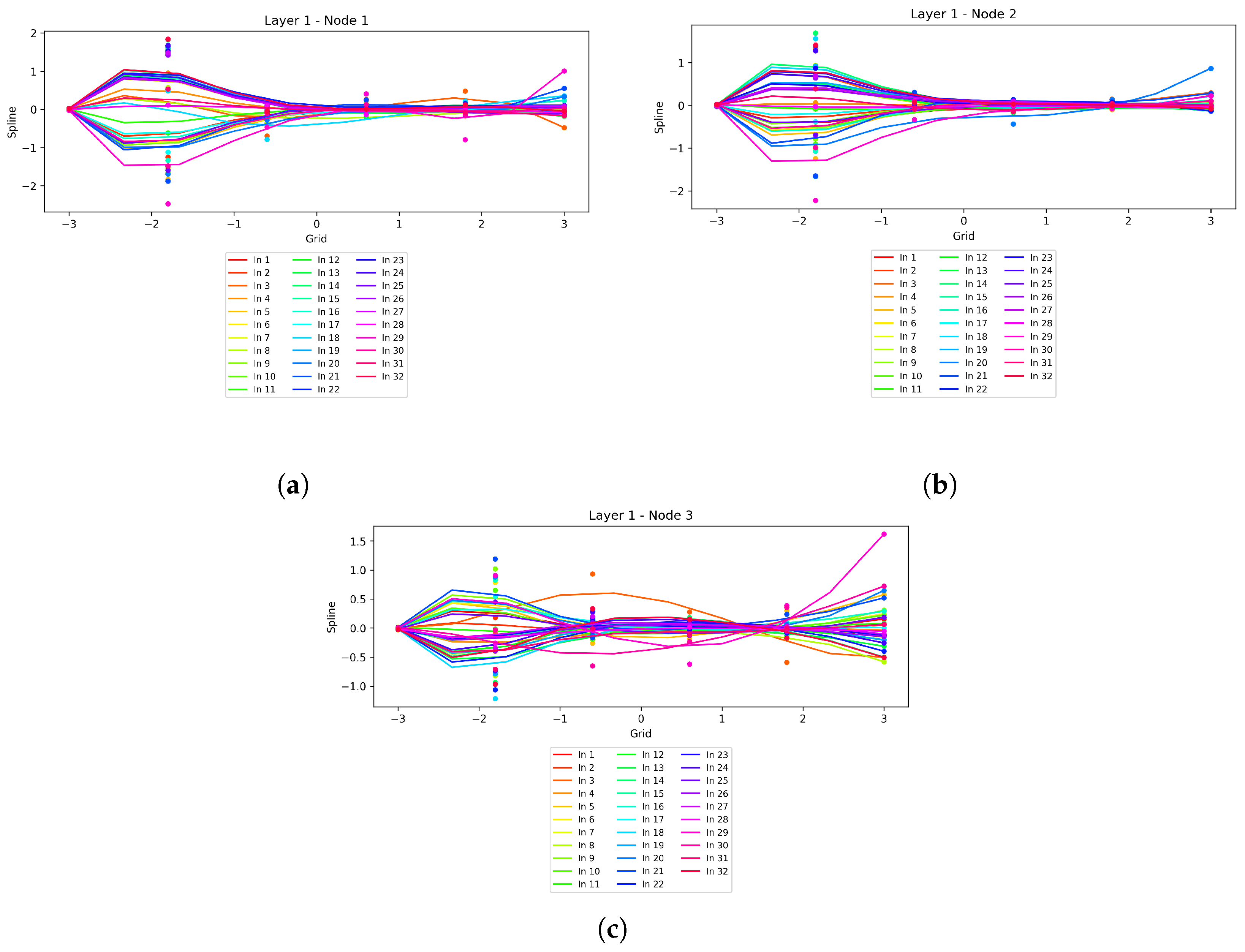
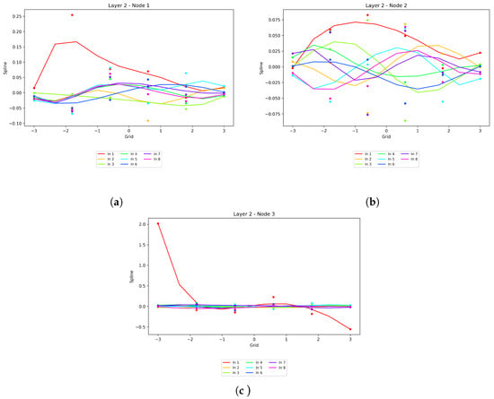
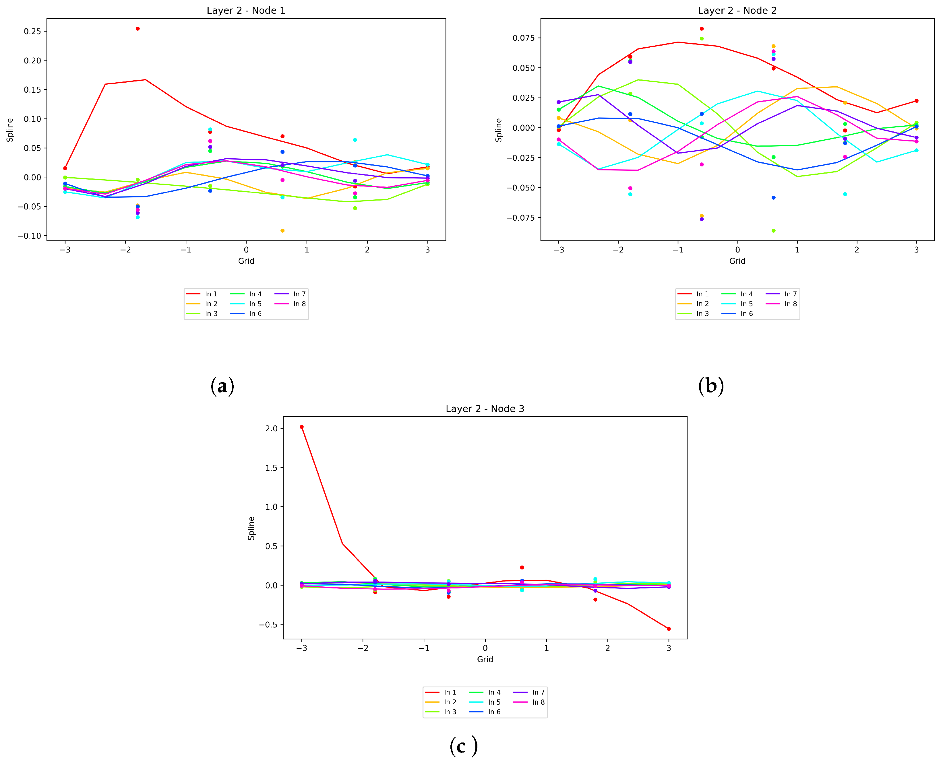
In general, the increased interpretability of KANs comes directly from their architecture, which replaces linear connections between neurons with parametric univariate spline functions learned from the data [16], acting along the network’s edges adapting dynamically its nonlinearity. KANs offer a significant advantage in terms of explainability because individual activation functions can be inspected. Each connection in the classic KAN has its own spline, coefficients, and grid of points that are learned during training. This structure is clearer, more understandable, and easier to visualize than traditional deep networks, also helping to reduce the total number of parameters [17]. The new F-QKAN and H-QKAN architectures inherit and leverage these advantages of transparency and structural interpretability. The F-QKAN, in particular, is inspired by the compositional structure of classic KANs: each layer can be interpreted as a univariate function (local rotation) followed by a composition of interactions (entanglement) [17]. Quantum rotations implement spline-like basis functions [15], while the IsingXX and CNOT operations represent the functional union of these components, similar to the hierarchical composition proposed by the Kolmogorov–Arnold theorem [15,16]. In the specific implementation of the H-QKAN model, a code block was created to graphically display the learned functions (Figure 14 and Figure 15).

Figure 14. Spline functions learned of Layer 1 of the H-QKAN. (a) Spline functions—Layer 1/Node 1. (b) Spline functions—Layer 1/Node 2. (c) Spline functions—Layer 1/Node 3.

Figure 15. Spline functions learned of Layer 2 of the H-QKAN. (a) Spline functions—Layer 2/Node 1. (b) Spline functions—Layer 2/Node 2. (c) Spline functions—Layer 2/Node 3.

Specifically, using the KAN layers, for each layer, the spline coefficients and grid points for each node were extracted. Using these parameters, the functions for each input connected to a specific node were reconstructed and drawn using the B-Spline implementation.

These graphs visually show how KAN modeled the nonlinear relationship between a specific input feature and the output activation of the intermediate node [15].

Specifically, each curve shows how an input is transformed by the node in question. The explainability comes from the fact that it’s possible to see the exact shape of the function used in each node, rather than treating it as a hidden entity: if the spline represented is almost a straight line, it means the transformation is almost linear and the model hasn’t added much complexity; if the spline is curved, it means that that node has learned a nonlinearity important for distinguishing classes.

The ability to visualize the exact shape of the function used in each node allows understanding of nonlinear relationships that would otherwise remain hidden.

4. Experimental Results and Discussion

Experiments conducted on classical, hybrid, and quantum models applied to the LFW dataset revealed differences in accuracy, computational efficiency, and stability during training, offering a rich and complex perspective on model behavior, learning dynamics, and practical tradeoffs.

The classical CNN model consistently achieved high levels of test accuracy and robust generalization, confirming its high discriminatory power. Epoch processing times were fast and stable, although training tended to require a larger number of epochs to achieve optimal performance. As a result, the overall training process was time-consuming and required careful management to mitigate the risk of overfitting. In absolute terms, CNN outperformed CKAN, especially with medium-resolution inputs (Table 2).

Table 2. Performance of training and testing metrics of implemented models for multiclass classification.

Model	Train Loss	Test Loss	Train Acc	Test Acc
CNN	0.3331	0.4370	0.9834	0.8682
CKAN	0.2102	0.6017	0.9600	0.8320

Integrating KAN into a convolutional architecture, as implemented in the CKAN model, resulted in slightly lower accuracy than CNN but significantly improved convergence behavior and reduced training time. The model demonstrated stable training dynamics while maintaining low test losses and showed improved performance when reducing input complexity, indicating good scalability to compressed visual features.

In the quantum domain, the QCNN model was able to learn nontrivial representations under ideal, noise-free conditions, achieving a test accuracy of approximately 77% (Table 3). However, the presence of quantum noise severely impacted learning, resulting in minimal accuracy improvements and erratic loss patterns.

Table 3. Performance of training and testing metrics of implemented models for binary classification.

Model	Train Loss	Test Loss	Train Acc	Test Acc
Noise-free QCNN	0.1697	0.1754	0.7799	0.7696
F-QKAN	0.6254	0.5826	0.7873	0.8043
H-QKAN	0.1189	0.2258	0.9590	0.9261

The fully quantum F-QKAN architecture outperformed QCNN, reaching a maximum test accuracy of 82.61% by the fifteenth epoch. This improvement came at the cost of extremely high computational requirements, as simulating a ten-level quantum circuit on a CPU required considerable runtime.

The hybrid H-QKAN network demonstrated good generalization capabilities and stable behavior over time. Its effectiveness was further confirmed by the confusion matrix, which showed a low error rate. Despite the inclusion of quantum components, the model converged quickly and maintained relatively manageable runtimes per epoch, even when simulating quantum circuits.

These results highlight several important considerations. While classical CNN models remain the most accurate, their computational cost and training time can be limiting. Hybrid approaches like CKAN represent an effective compromise, particularly in scenarios where inference speed and resource constraints are critical. In the quantum domain, noise emerges as the primary limiting factor, underscoring the need for architectures that can tolerate or mitigate its effects. Hybrid solutions that integrate quantum levels within classical frameworks appear to be a promising direction, combining classical stability with the representational potential of quantum models.

A common aspect of CKANs, F-QKANs, and H-QKANs is their explainability. KANs aims to reduce “black boxes” by replacing linear connections with parametric spline functions learned directly from the data. This allows us to examine what the network has learned: quasi-linear spline functions indicate limited additional complexity, while highly curved splines reveal critical nonlinear transformations. Architectures like H-QKANs allow these functions to be visualized and reconstructed, providing insights into nonlinear relationships that would otherwise remain hidden. This transparency is valuable not only for interpretability, but also for debugging and improving the model.

Overall, the evaluation of the implemented neural architectures suggests that the optimal model choice depends on task-specific requirements, such as accuracy, explainability, computational efficiency, and scalability. For multiclass classification (Table 2), CNN offers the highest predictive reliability at the expense of complexity, while hybrid models such as CKAN provide a balanced alternative with faster training and good scalability to low-resolution inputs. For binary classification (Table 3), H-QKAN emerges as the most effective solution, combining high generalization, stability, and efficiency with structural transparency. Pure quantum networks, although currently slow and susceptible to noise, remain an important avenue for future research. In this context, F-QKAN demonstrates that the principles of KAN can be successfully extended to fully quantum architectures, while H-QKAN stands out as a practical and well-balanced approach despite current technological constraints.

5. Conclusions and Future Directions

This work offers an in-depth comparative analysis of different image classification, architectures: for multiclass classification CNNs and CKANs are compared; for binary classification, QCNNs, F-QKANs and H-QKANs are compared, applied to the well-known LFW dataset.

Each model represents a different computational philosophy, ranging from the maturity of classical DL to the more recent perspectives offered by quantum and hybrid computing.

CNN-based models have confirmed their effectiveness and maturity, consistently achieving high accuracy and robust generalization, proving suitable for real world implementation. The main limitation remains computational cost and training complexity, which can be significant when dealing with large datasets or high-resolution inputs.

In contrast, KAN-based architectures, particularly CKAN, have demonstrated significant advantages in terms of computational efficiency and model interpretability, making them attractive in scenarios where transparency and reduced computational costs are crucial.

For binary classification, in the quantum domain, QCNN confirmed the theoretical potential of architectures based on variable quantum circuits, although it still failed to compete with classical models in realistic, noisy conditions. However, in ideal, noise-free environments, it demonstrated the ability to learn nontrivial representations.

The F-QKAN represented an ambitious attempt to fully transpose the framework based on Kolmogorov–Arnold theory to a Quantum Computing (QC) context. Despite the high computational cost of simulating a ten-layer quantum circuit, the model outperformed QCNN. This result demonstrates how the structural principles of KANs can be effectively adapted to variable quantum circuits, opening up promising prospects for future applications on more mature quantum hardware.

The H-QKAN architecture emerged as the most balanced and promising solution among all those analyzed in relation to the binary classification experiment. By combining a classical KAN-based feature extractor with a variational quantum classifier, it achieved excellent generalization capabilities and remarkable stability. Of particular note is its computational efficiency: despite the presence of a simulated quantum circuit, the model showed rapid convergence and a low execution time per epoch, confirming its position as an extremely competitive solution for hybrid quantum–classical computing.

Future research should focus on several directions. First, it will be important to optimize the scalability and explainability of KAN-based architectures by applying them to larger and more complex data sets. At the same time, the robustness of quantum circuits to noise and hardware imperfections will need to be improved through the adoption of advanced error migration strategies. Finally, a further line of investigation could involve the exploration of novel hybrid schemes capable of dynamically integrating classical and quantum components, thus fully exploiting the potential of both technologies.

In addition, several important directions emerge from the present study and from the discussion of its limitations. First, although robustness considerations were not the main focus of this work, an evaluation of adversarial robustness across classical, spline-based, and hybrid quantum architectures represents a relevant and open research direction.

Second, to further clarify the specific contribution of the quantum component within the H-QKAN architecture, future work should include dedicated ablation studies comparing the hybrid model against purely classical baselines operating on the same PCA-reduced feature space, such as a classical KAN followed by a softmax or multilayer perceptron classifier. Such comparisons are useful for examinig the impact of quantum variational layers in those hybrid architectures.

Overall, the results presented in this study suggest that hybrid quantum–classical architectures represent a promising research direction rather than a mature alternative to established deep learning solutions. While further validation is required, these findings motivate continued investigation into hybrid designs as a viable and flexible paradigm for future quantum-aware machine-learning research.

References

- Huang, S.Y.; An, W.J.; Zhang, D.S.; Zhou, N.R. Image classification and adversarial robustness analysis based on hybrid quantum–classical convolutional neural network. Opt. Commun. 2023, 533, 129287. [Google Scholar] [CrossRef] [Scilit]
- Smaldone, A.M.; Kyro, G.W.; Batista, V.S. Quantum convolutional neural networks for multi-channel supervised learning. Quantum Mach. Intell. 2023, 5, 41. [Google Scholar] [CrossRef] [Scilit]
- Napoli, F.; Castaldo, M.; Marrone, S.; Campanile, L. Comparing Emerging Technologies in Image Classification: From Quantum to Kolmogorov. In Proceedings of the International Conference on Computational Science and Its Applications, Istanbul, Türkiye, 30 June–3 July 2025; Springer: Cham, Switzerland, 2025; pp. 260–273. [Google Scholar]
- Huang, G.B.; Mattar, M.; Berg, T.; Learned-Miller, E. Labeled faces in the wild: A database for studying face recognition in unconstrained environments. In Proceedings of the Workshop on Faces in ’Real-Life’ Images: Detection, Alignment, and Recognition, Marseille, France, 17 October 2008. [Google Scholar]
- Krizhevsky, A.; Sutskever, I.; Hinton, G.E. Imagenet classification with deep convolutional neural networks. Adv. Neural Inf. Process. Syst. 2012, 25, 84–90. [Google Scholar] [CrossRef] [Scilit]
- Simonyan, K.; Zisserman, A. Very deep convolutional networks for large-scale image recognition. arXiv 2014, arXiv:1409.1556. [Google Scholar]
- He, K.; Zhang, X.; Ren, S.; Sun, J. Deep residual learning for image recognition. In Proceedings of the IEEE Conference on Computer Vision and Pattern Recognition, Las Vegas, NV, USA, 27–30 June 2016; pp. 770–778. [Google Scholar]
- Rawat, W.; Wang, Z. Deep convolutional neural networks for image classification: A comprehensive review. Neural Comput. 2017, 29, 2352–2449. [Google Scholar] [CrossRef] [Scilit]
- Gupta, P.; Saxena, N.; Sharma, M.; Tripathi, J. Deep neural network for human face recognition. Int. J. Eng. Manuf. (IJEM) 2018, 8, 63–71. [Google Scholar] [CrossRef] [Scilit]
- Goodfellow, I.J.; Shlens, J.; Szegedy, C. Explaining and harnessing adversarial examples. arXiv 2014, arXiv:1412.6572. [Google Scholar]
- Liu, Z.; Wang, Y.; Vaidya, S.; Ruehle, F.; Halverson, J.; Soljačić, M.; Hou, T.Y.; Tegmark, M. Kan: Kolmogorov-arnold networks. arXiv 2024, arXiv:2404.19756. [Google Scholar] [PubMed]
- Cheon, M. Kolmogorov-Arnold Network for Satellite Image Classification in Remote Sensing. arXiv 2024, arXiv:2406.00600. [Google Scholar] [CrossRef] [Scilit]
- Wang, Z.; Zainal, A.; Siraj, M.M.; Ghaleb, F.A.; Hao, X.; Han, S. An intrusion detection model based on Convolutional Kolmogorov-Arnold Networks. Sci. Rep. 2025, 15, 1917. [Google Scholar] [CrossRef] [Scilit]
- Zheng, H.; Su, H.; Wu, Z.; Chen, Y.; Du, Q. Graph Kolmogorov-Arnold Convolutional Network for Hyperspectral Image Classification. IEEE J. Sel. Top. Appl. Earth Obs. Remote Sens. 2025, 18, 14738–14751. [Google Scholar] [CrossRef] [Scilit]
- Ivashkov, P.; Huang, P.W.; Koor, K.; Pira, L.; Rebentrost, P. QKAN: Quantum Kolmogorov-Arnold Networks. arXiv 2024, arXiv:2410.04435. [Google Scholar] [CrossRef] [Scilit]
- Daskin, A. Quantum Kolmogorov-Arnold networks by combining quantum signal processing circuits. arXiv 2024, arXiv:2410.04218. [Google Scholar] [CrossRef] [Scilit]
- Kundu, A.; Sarkar, A.; Sadhu, A. Kanqas: Kolmogorov-arnold network for quantum architecture search. EPJ Quantum Technol. 2024, 11, 76. [Google Scholar] [CrossRef] [Scilit]
- Wakaura, H.; Mulyawan, R.; Suksmono, A.B. Adaptive Variational Quantum Kolmogorov-Arnold Network. arXiv 2025, arXiv:2503.21336. [Google Scholar]
- Schuld, M.; Petruccione, F. Machine Learning with Quantum Computers; Springer: Berlin/Heidelberg, Germany, 2021; Volume 676. [Google Scholar]
- Cong, I.; Choi, S.; Lukin, M.D. Quantum convolutional neural networks. Nat. Phys. 2019, 15, 1273–1278. [Google Scholar] [CrossRef] [Scilit]
- Hur, T.; Kim, L.; Park, D.K. Quantum convolutional neural network for classical data classification. Quantum Mach. Intell. 2022, 4, 3. [Google Scholar] [CrossRef] [Scilit]
- Wei, S.; Chen, Y.; Zhou, Z.; Long, G. A quantum convolutional neural network on NISQ devices. AAPPS Bull. 2022, 32, 2. [Google Scholar] [CrossRef] [Scilit]
- Song, Y.; Li, J.; Wu, Y.; Qin, S.; Wen, Q.; Gao, F. A resource-efficient quantum convolutional neural network. Front. Phys. 2024, 12, 1362690. [Google Scholar] [CrossRef] [Scilit]
- Roh, E.J.; Im, C.; Jeong, W.; Park, S. Computation-efficient quantum convolutional neural networks for autonomous driving applications: EJ Roh et al. J. Supercomput. 2025, 81, 1033. [Google Scholar] [CrossRef] [Scilit]
- Umeano, C.; Paine, A.E.; Elfving, V.E.; Kyriienko, O. What can we learn from quantum convolutional neural networks? Adv. Quantum Technol. 2025, 8, 2400325. [Google Scholar] [CrossRef] [Scilit]
- Ranga, D.; Prajapat, S.; Akhtar, Z.; Kumar, P.; Vasilakos, A.V. Hybrid quantum–classical neural networks for efficient MNIST binary image classification. Mathematics 2024, 12, 3684. [Google Scholar] [CrossRef] [Scilit]
- Hafeez, M.A.; Munir, A.; Ullah, H. H-QNN: A hybrid quantum–classical neural network for improved binary image classification. AI 2024, 5, 1462–1481. [Google Scholar] [CrossRef] [Scilit]
- Zaman, K.; Ahmed, T.; Hanif, M.A.; Marchisio, A.; Shafique, M. A comparative analysis of hybrid-quantum classical neural networks. In Proceedings of the World Congress in Computer Science, Computer Engineering & Applied Computing, Las Vegas, NV, USA, 22–25 July 2024; Springer: Cham, Switzerland, 2024; pp. 102–115. [Google Scholar]
- Somvanshi, S.; Javed, S.A.; Islam, M.M.; Pandit, D.; Das, S. A Survey on Kolmogorov-Arnold Network. ACM Comput. Surv. 2025, 58, 55. [Google Scholar] [CrossRef] [Scilit]
- LeCun, Y.; Bengio, Y. Convolutional networks for images, speech, and time series. In The Handbook of Brain Theory and Neural Networks; MIT Press: Cambridge, MA, USA, 1995; Volume 3361, pp. 255–258. [Google Scholar]
- Goodfellow, I.; Bengio, Y.; Courville, A.; Bengio, Y. Deep Learning; MIT Press: Cambridge, MA, USA, 2016. [Google Scholar]
- Kingma, D.P. Adam: A method for stochastic optimization. arXiv 2014, arXiv:1412.6980. [Google Scholar]
- Rumelhart, D.E.; Hinton, G.E.; Williams, R.J. Learning representations by back-propagating errors. Nature 1986, 323, 533–536. [Google Scholar] [CrossRef] [Scilit]
Disclaimer/Publisher’s Note: The statements, opinions and data contained in all publications are solely those of the individual author(s) and contributor(s) and not of MDPI and/or the editor(s). MDPI and/or the editor(s) disclaim responsibility for any injury to people or property resulting from any ideas, methods, instructions or products referred to in the content. |
© 2026 by the authors. Licensee MDPI, Basel, Switzerland. This article is an open access article distributed under the terms and conditions of the Creative Commons Attribution (CC BY) license.