Impact of Neural Network Initialisation Seed and Architecture on Accuracy, Generalisation and Generative Consistency in Data-Driven Internal Combustion Engine Modelling

Abstract

Artificial neural networks (ANNs) are widely used to approximate nonlinear mappings, yet their ability to capture thermodynamic behaviour in dynamic physical systems remains insufficiently characterised. This study investigates how representational capacity influences surrogate modelling accuracy for a crank-angle-resolved internal combustion engine (ICE) simulation with a maximum dynamic state dimension of six. Two feedforward ANN configurations are evaluated: a low-capacity 5–5 architecture containing 84 trainable parameters and a high-capacity 25–25–25 architecture containing 1554 parameters (18.5× larger). Both networks approximate the nonlinear mapping from five embedded operating parameters to four peak thermodynamic outputs (maximum pressure, pressure phasing, maximum temperature, and temperature phasing). Evaluation across 53,178 operating points demonstrates that the high-capacity configuration reduces root mean squared error by factors of 30–50× relative to the low-capacity network, decreasing peak temperature error from 17.68 K to 0.36 K and peak pressure error from 0.116 MPa to 0.0025 MPa. Although both models achieve coefficients of determination exceeding 0.99, the low-capacity network exhibits heavy-tailed residual distributions and regime-dependent error amplification, whereas the high-capacity model reduces both central dispersion and extreme-case error. These results demonstrate that high correlation alone does not guarantee engineering reliability in nonlinear thermodynamic systems. Distribution-level analysis, including percentile and extreme-case characterisation, is required to evaluate engineering robustness. The findings provide a quantitative framework linking ANN capacity, nonlinear dynamic system representation, and predictive robustness.

1. Introduction

Internal combustion engines (ICEs) remain a cornerstone of global transportation and energy conversion, continuing to power a large share of road vehicles worldwide despite the rapid expansion of electrified powertrains [1,2,3]. Their persistence is driven by high power density, established manufacturing infrastructure, and broad fuel compatibility, particularly in sectors such as heavy-duty transport, marine propulsion, and off-highway applications where full electrification remains constrained by system-level limitations including energy density, cost, and infrastructure limitations [1,2]. At the same time, ICE technology has entered a mature and transitional phase, shaped by increasingly stringent emissions legislation and a gradual shift toward hybridised and fuel-flexible architectures rather than standalone combustion systems [4,5].

Regulatory frameworks such as the European Union’s forthcoming Euro 7 standard impose substantially lower limits on nitrogen oxides, particulate matter, and other regulated pollutants [4]. These constraints have reshaped the research landscape, placing renewed emphasis on extracting higher efficiency and cleaner combustion from increasingly constrained systems [4,5]. In response, contemporary ICE development has shifted away from incremental mechanical optimisation alone and toward system-level strategies that combine advanced combustion concepts, alternative fuels, hybridisation, and intelligent control [5,6,7,8]. Hydrogen, biofuels, and synthetic e-fuels are increasingly viewed in the recent ICE literature as transitional enablers that extend ICE relevance while broader electrification infrastructure continues to mature [6,7].

Within this evolving context, computational modelling has become an essential tool for understanding and optimising engine behaviour across wide operating envelopes [9,10]. High-fidelity approaches such as three-dimensional computational fluid dynamics (CFD) offer deep physical insight but often remain computationally prohibitive for large-scale parametric studies, real-time control, or iterative design workflows [11,12]. Even reduced-order physics-based models, while more tractable, impose non-negligible computational costs when explored over high-dimensional design spaces (e.g., multi-parameter sweeps over speed, load, timing, EGR, and fuel composition) [9,10]. These limitations have motivated growing interest in surrogate modelling approaches capable of approximating engine behaviour at a fraction of the computational expense [12,13,14].

Surrogate models aim to learn mappings between engine operating parameters and key combustion outcomes, enabling rapid prediction without repeated evaluation of the underlying physical model [12,13,14]. While effective for low-dimensional problems, classical regression and response-surface approaches can struggle to capture the strong nonlinearities and coupled dependencies inherent to combustion systems [12,14,15]. More recently, machine-learning-based surrogates, particularly artificial neural networks (ANNs), have emerged as powerful alternatives, demonstrating the ability to approximate complex engine responses with high accuracy while achieving computational speed-ups from approximately 45 to 70 compared to repeated evaluations of the underlying physics-based model [16,17,18].

ANN-based surrogates are increasingly proposed for applications ranging from design space exploration and virtual sensing to optimisation and real-time control, and are often viewed as enabling components of digital twins for combustion systems [14,18,19,20,21]. However, despite their growing adoption, important questions remain regarding surrogate reliability [18]. In practical engineering workflows, surrogate models are frequently used not only for pointwise prediction but also for dataset generation, sensitivity analysis, and exploratory sampling across operating regimes [14,15]. In these contexts, surrogate quality cannot be assessed solely through aggregate accuracy metrics such as correlation-based measures, as models may exhibit strong global fit while still producing large absolute errors, regime-dependent bias, or distortion of the underlying data structure when used generatively [22].

One aspect that remains comparatively under-examined in ANN surrogate studies is the role of network capacity [23]. While increased depth or width is often assumed to improve performance, the extent to which representational capacity influences convergence behaviour, robustness across operating regimes, and preservation of the underlying physics-generated data structure remains insufficiently quantified [14,15,16,17,18]. Moreover, stochastic elements such as weight initialisation and optimisation can interact with architecture in non-trivial ways, further complicating surrogate selection [24,25]. These factors are particularly relevant when surrogates are trained on physics-generated datasets, where the learned mapping reflects not experimental noise but structured nonlinear relationships imposed by conservation laws and thermodynamic constraints [9,10].

The present study addresses these gaps through a controlled, systematic evaluation of ANN surrogate models with differing representational capacity, trained on a high-resolution, crank-angle-resolved thermodynamic engine dataset generated using a zero-dimensional MATLAB-based simulation framework [9,10]. Two representative surrogate configurations are examined: a low-capacity network and a high-capacity network, selected from a comprehensive architecture–initialisation sweep and trained under identical data partitioning, preprocessing, and optimisation conditions [25,26]. This controlled setup enables direct attribution of observed performance differences to architectural capacity rather than confounding factors [25].

Unlike many prior studies that focus primarily on pointwise prediction accuracy [16,17,18], this work adopts a multifaceted evaluation framework. In addition to standard regression metrics, the analysis examines training convergence behaviour, residual structure across the operating domain, error distribution tails, and the ability of each surrogate to preserve the statistical and geometric structure of the physics-generated dataset under generative sampling [14,22]. This broader perspective is essential for assessing whether an ANN surrogate is suitable not only as a fast predictor but also as a reliable stand-in for the underlying physical model in exploratory and generative workflows [14,15].

By explicitly contrasting the behaviour of capacity-limited and high-capacity ANN surrogates, this study establishes practical criteria for surrogate reliability in combustion modelling applications [14,18]. The findings demonstrate how high-correlation metrics alone can be misleading [22], clarify how insufficient capacity manifests as regime-dependent error and distributional distortion [14,15], and identify conditions under which ANN surrogates can faithfully reproduce both the accuracy and structure of physics-based engine simulations [9,10].

Preliminary experiments investigated several modelling approaches for predicting combustion characteristics from the generated simulation dataset. A simple linear regression baseline confirmed that linear models cannot adequately represent the highly nonlinear relationships inherent to combustion processes, motivating the use of artificial neural networks.

The present study extends that preliminary work presented in [27] by introducing dataset cleaning procedures, a structured parameter sweep covering 61,875 operating conditions, and improved preprocessing techniques. In addition, two neural network architectures are systematically evaluated to investigate how model design influences predictive accuracy and reliability. These improvements enable a more systematic investigation of the influence of neural network architecture on combustion prediction performance. The novelty of this work lies in the systematic evaluation of how neural network architecture capacity and weight initialisation influence the reliability of surrogate models for crank-angle-resolved thermodynamic engine simulations.

2. Methods

2.1. Engine Model

The zero-dimensional engine model is formulated as a crank-angle-resolved thermodynamic simulation implemented in MATLAB R2025b. The in-cylinder charge is represented as a spatially uniform control volume, and its thermodynamic state evolves according to conservation of mass and energy. The crank angle is used as the independent variable, enabling direct coupling between piston kinematics and thermodynamic evolution.

The four-stroke engine cycle is decomposed into intake, compression, combustion, and expansion phases. Within each phase, the relevant physical processes are activated through dedicated rate formulations. Gas exchange and blow-by are represented using simplified mass-flow sub-models, while combustion is prescribed using a smooth half-cosine mass-fraction-burned function. This formulation provides numerical stability and captures the dominant thermodynamic trends required for parametric analysis without requiring spatial resolution.

Thermodynamic and transport properties are evaluated using mixture-dependent relations accounting for equivalence ratio, fuel composition, and temperature. During combustion, a two-zone approximation is employed to represent burned and unburned regions within the control volume.

Prior to dataset generation, the MATLAB-based zero-dimensional model was cross-compared against established commercial engine simulation environments, including a three-dimensional CFD combustion solver (ANSYS Forte) and a one-dimensional system-level engine modelling platform (GT-SUITE), as detailed in [9,10]. Agreement was evaluated in terms of in-cylinder pressure traces, temperature evolution, and combustion phasing metrics. These cross-comparisons confirmed that the simplified thermodynamic formulation captures the dominant physical trends required for data-driven modelling applications.

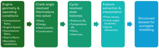
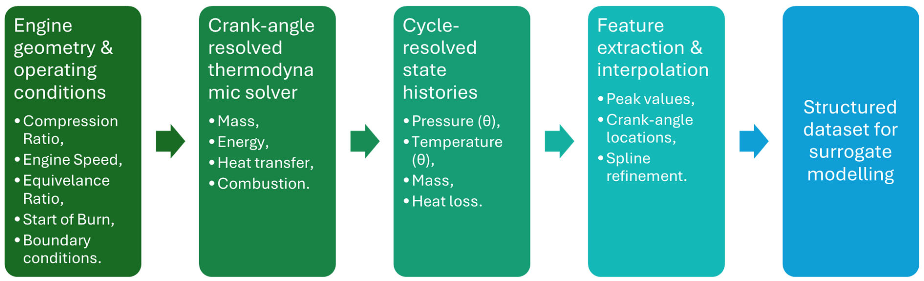
Figure 1 illustrates the conceptual structure of the zero-dimensional simulation and its integration within the dataset generation workflow.

Figure 1. Conceptual structure of the zero-dimensional engine simulation and dataset generation pipeline.

Cylinder volume is

$$V\left(\mathsf{\theta }\right)=V_{\mathrm{T}\mathrm{D}\mathrm{C}}\left[1+{\displaystyle \frac{r-1}{2}}\left(1-\mathrm{c}\mathrm{o}\mathrm{s}\mathsf{\theta }+\left({\displaystyle \frac{1}{\epsilon }}\right)\left(1-\sqrt{1-{\epsilon }^2\mathrm{s}\mathrm{i}{\mathrm{n}}^2\mathsf{\theta }}\right)\right)\right],$$

(1)

where V(θ) is instantaneous cylinder volume, V_TDC is clearance volume at top dead centre, θ is crank angle measured from TDC, r is geometric compression ratio, and ε is ratio of crank radius to connecting rod length. Equation (1) defines the instantaneous cylinder volume as a function of crank angle θ, derived from slider–crank kinematics. Its derivative with respect to θ is used to compute the pressure–volume work term in the energy equation.

Ideal gas law is used to link density, pressure and temperature

$$pV=mRT,$$

(2)

where p is in-cylinder pressure, V is cylinder volume, m is in-cylinder gas mass, R is specific gas constant of the mixture, and T is in-cylinder gas temperature. The ideal gas law provides thermodynamic closure for the in-cylinder control volume, relating pressure, volume, temperature, and mass. Mixture-dependent gas properties are used for R.

Mass conservation with blow-by is found from the equation

$${\displaystyle \frac{dm}{d\mathsf{\theta }}}=-\left({\displaystyle \frac{C_{bb}}{\omega }}\right)m,$$

(3)

where m is in-cylinder mass, θ is crank angle, C_bb is blow-by coefficient, and ω is engine angular speed. This equation models blow-by losses using a simplified exponential formulation with respect to crank angle.

First law of thermodynamics is written as

$${\displaystyle \frac{dU}{d\mathsf{\theta }}}=\left({\displaystyle \frac{1}{\omega }}\right)\left({\dot{Q}}_{comb}-{\dot{Q}}_{wall}\right)-p·{\displaystyle \frac{dV}{d\mathsf{\theta }}}+\left({\displaystyle \frac{1}{\omega }}\right)\Sigma \left({\dot{m}}_{in}{h}_{in}-{\dot{m}}_{out}{h}_{out}\right)-\left({\displaystyle \frac{1}{\omega }}\right){\dot{m}}_{bb}{h}_{bb},$$

(4)

where U is total internal energy of the cylinder charge, ${\dot{Q}}_{comb}$ is rate of heat release due to combustion, ${\dot{Q}}_{wall}$ is rate of heat transfer to cylinder walls, p is in-cylinder pressure, V is cylinder volume, ${\dot{m}}_{in}$ is mass flow rate into the cylinder, ${\dot{m}}_{out}$ is mass flow rate out of the cylinder, h_in is specific enthalpy of incoming gas, h_out is specific enthalpy of outgoing gas, ${\dot{m}}_{bb}$ is blow-by mass flow rate, h_bb is specific enthalpy of blow-by gas, and ω is engine angular speed. This is the governing energy balance for the cylinder control volume. It accounts for combustion heat release, wall heat transfer, pressure–volume work, gas exchange enthalpy flows, and blow-by losses.

Mass fraction burned is found as

$$x_{b\left(\theta \right)}=0.5\left[1-\cos \left({\displaystyle \frac{\pi \left(\mathsf{\theta }-{\mathsf{\theta }}_s\right)}{{\mathsf{\theta }}_b}}\right)\right],$$

(5)

where x_b is mass fraction of burned mixture, θ is crank angle, θ_s is start of combustion crank angle, and θ_b is total combustion duration. A smooth half-cosine burn law is used to prescribe the progression of combustion between start of combustion θ_s and burn duration θ_b, chosen for its numerical smoothness and ability to represent generic spark-ignition heat-release profiles without introducing additional fitting parameters. Its derivative defines the heat-release rate.

Wall heat transfer is expressed in the form

$${\dot{Q}}_{wall}=hA\left(T-T_w\right),$$

(6)

where h is convective heat transfer coefficient, A is instantaneous heat transfer surface area, T is in-cylinder gas temperature, and T_w is cylinder wall temperature. This equation models convective heat transfer between the in-cylinder gases and the combustion chamber walls. The heat transfer coefficient h may be constant or computed using a Woschni-type correlation.

The crank-angle-resolved engine model can be expressed in dynamical form as

$${\displaystyle \frac{dx}{d\mathsf{\theta }}}=F(x,u)$$

(7)

where $\mathsf{\theta }$ is crank angle (rad), $x$ denotes the dynamic state vector, and $u$ represents the operating parameter vector defining each simulation case.

The maximum dynamic state dimension occurs during the two-zone combustion phase. The state vector is defined as

$$x(\mathsf{\theta })=\left[\begin{array}{c}p\left(\mathsf{\theta }\right)\\ T_u\left(\mathsf{\theta }\right)\\ T_b\left(\mathsf{\theta }\right)\\ W\left(\mathsf{\theta }\right)\\ Q_{wall}\left(\mathsf{\theta }\right)\\ Q_{leak}\left(\mathsf{\theta }\right)\end{array}\right]\in {\mathbb{R}}^6$$

(8)

where $p$ is in-cylinder pressure (Pa), $T_u$ is unburned gas temperature (K), $T_b$ is burned gas temperature (K), $W$ is cumulative indicated work (J), $Q_{wall}$ is cumulative wall heat transfer (J), and $Q_{leak}$ represents cumulative heat leakage (J). The maximum state dimension is therefore

$$\mathrm{d}\mathrm{i}\mathrm{m}\left(x\right)=6$$

(9)

Other phases of the engine cycle involve between three and five state variables depending on the thermodynamic regime. Despite strong nonlinear thermodynamic coupling, the underlying physical system remains low-dimensional in state space.

The operating parameter vector defining each simulation case is

$$\mathrm{u}=\left[\begin{array}{c}\varphi \\ \mathrm{RPM}\\ r\\ {\mathsf{\theta }}_{\mathrm{S}\mathrm{o}\mathrm{B}}\end{array}\right]\in {\mathbb{R}}^4$$

(10)

where $\varphi$ is equivalence ratio, $\mathrm{R}\mathrm{P}\mathrm{M}$ is engine speed, $r$ is geometric compression ratio, and ${\mathsf{\theta }}_{\mathrm{S}\mathrm{o}\mathrm{B}}$ is start-of-burn crank angle (deg).

To preserve angular continuity in the regression framework, the start-of-burn angle is embedded using sine and cosine encoding, yielding

$${\mathrm{u}}_{\mathrm{e}\mathrm{m}\mathrm{b}\mathrm{e}\mathrm{d}}=\left[\begin{array}{c}\varphi \\ \mathrm{RPM}\\ r\\ \sin \left({\mathsf{\theta }}_{\mathrm{S}\mathrm{o}\mathrm{B}}\right)\\ \cos \left({\mathsf{\theta }}_{\mathrm{S}\mathrm{o}\mathrm{B}}\right)\end{array}\right]\in {\mathbb{R}}^5$$

(11)

Thus, the ANN input dimension is five.

The regression targets correspond to peak thermodynamic quantities,

$$\mathrm{y}=\left[\begin{array}{c}{\mathrm{M}\mathrm{a}\mathrm{x}\mathrm{P}}_{\mathrm{M}\mathrm{P}\mathrm{a}}\\ {\mathrm{C}\mathrm{A}@\mathrm{M}\mathrm{a}\mathrm{x}\mathrm{P}}_{\mathrm{d}\mathrm{e}\mathrm{g}}\\ {\mathrm{M}\mathrm{a}\mathrm{x}\mathrm{T}}_{\mathrm{K}}\\ {\mathrm{C}\mathrm{A}@\mathrm{M}\mathrm{a}\mathrm{x}\mathrm{T}}_{\mathrm{d}\mathrm{e}\mathrm{g}}\end{array}\right]\in {\mathbb{R}}^4$$

(12)

where $\mathrm{M}\mathrm{a}\mathrm{x}\mathrm{P}$ is peak cylinder pressure, $\mathrm{M}\mathrm{a}\mathrm{x}\mathrm{T}$ is peak cylinder temperature, and $\mathrm{C}\mathrm{A}$ denotes the crank-angle location of each maximum. The output dimension is therefore four.

Although the dynamical system has a maximum internal state dimension of six, the induced nonlinear mapping from operating parameters to peak outputs exhibits sufficient curvature to challenge low-capacity surrogate models.

These equations represent the governing conservation laws and constitutive relations underlying the numerical implementation. In the MATLAB model they are rearranged into crank-angle-resolved ordinary differential equations and integrated numerically for each engine cycle phase. The model provides deterministic, physically consistent cycle simulations for a given set of operating conditions across a wide operating envelope, forming a reliable foundation for large-scale dataset generation.

2.2. Dataset Generation and Feature Extraction

The parameter space was initially discretised using predefined ranges and uniform step increments across equivalence ratio (φ), engine speed (RPM), compression ratio (r), and start-of-burn timing. The resulting full-factorial sweep generated raw simulation outputs for all parameter combinations. The parameter sweep covered equivalence ratio φ = 0.5–1.5 (step 0.1), engine speed 600–3000 RPM (step 100 RPM), compression ratio 6–14 (step 1), and start-of-burn timing −50° to 10° (step 2.5°), producing a total of 61,875 simulation cases. The dataset was subsequently screened for numerical stability and physical consistency. Entries containing undefined or non-physical values (e.g., NaNs arising from thermodynamic divergence under extreme operating conditions) were excluded, removing 8697 unstable operating points and yielding a final dataset of 53,178 valid samples used for ANN training and evaluation.

Table 1 and Table 2 summarise representative subsets of the final cleaned dataset. Table 1 presents the input parameter combinations defining each simulated operating condition, while Table 2 reports the corresponding extracted cycle-level response quantities. Each row represents one complete engine cycle simulation evaluated under a unique set of operating parameters.

Table 1. Generated dataset inputs (representative subset).

No	Equivalence Ratio (φ)	Engine Speed (RPM)	Compression Ratio (r)	Start-of-Burn (deg)
1	0.5	600	6	−50
2	0.6	600	6	−50
3	0.7	600	6	−50
4	0.8	600	6	−50
5	0.9	600	6	−50
…	…	…	…	…
53,174	0.8	3000	14	−2.5
53,175	0.9	3000	14	−2.5
53,176	1	3000	14	−2.5
53,177	1.2	3000	14	−2.5
53,178	1.3	3000	14	−2.5

Table 2. Generated dataset outputs (representative subset).

No	Max Pressure (MPa)	Crank Angle at Max Pressure (deg)	Max Temperature (K)	Crank Angle at Max Temperature (deg)
1	3.0625	2.9838	1868.5090	−3.4730
2	3.3884	3.1906	2058.5641	−3.5809
3	3.6959	3.3633	2234.3243	−3.6367
4	3.9833	3.5270	2393.6745	−3.5917
5	4.2415	3.7122	2528.6891	−3.3633
…	…	…	…	…
53,174	3.5471	13.8525	2284.9987	10.8975
53,175	3.6344	16.7554	2412.8200	13.4730
53,176	3.7144	18.6906	2500.8082	15.2230
53,177	3.6880	19.3094	2414.5012	15.5486
53,178	3.6422	19.2014	2333.3289	15.4622

For each simulated operating point, characteristic output quantities including peak pressure, peak temperature, and their corresponding crank-angle locations are extracted from the simulated state histories. To avoid discretisation artefacts arising from fixed crank-angle resolution, a spline-based interpolation is applied to the pressure and temperature traces prior to feature extraction. This approach preserves the physical shape of the cycle while enabling sub-resolution localisation of extrema without the computational cost of uniformly reducing the integration step size. The resulting procedure improves numerical consistency across parameter combinations and yields a more informative dataset for subsequent surrogate modelling.

Although the zero-dimensional thermodynamic model provides physically consistent cycle simulations, direct evaluation remains computationally demanding when exploring large parametric spaces. The mapping between operating parameters and cycle-level outputs is highly nonlinear due to coupled thermodynamic and combustion interactions. To enable rapid prediction of these key quantities across the explored operating domain, artificial neural networks were trained using the generated dataset. The configuration and evaluation of the ANN models are described in the following section.

2.3. Data-Driven ANN Model Architecture and Training Framework

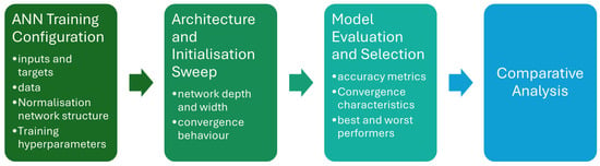
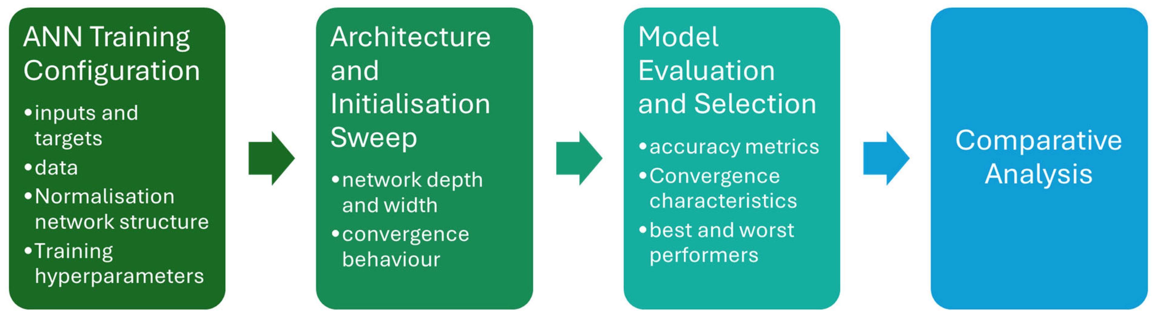
The overall data-driven modelling workflow, including ANN training, architecture variation and model selection, is summarised in Figure 2. While the present section focuses on the base ANN architecture and fixed training configuration, the subsequent section describes the structured architecture–initialisation sweep and selection procedure in detail.

Figure 2. ANN training, sweep, and model selection workflow.

The modelling workflow was implemented in MATLAB using a custom training routine designed to ensure strict reproducibility and distinct separation of stochastic effects. The problem was formulated as a supervised regression task where a feedforward artificial neural network approximated the nonlinear mapping between the engine operating parameters and the cycle-level response quantities.

To resolve the numerical discontinuity associated with angular data, the start-of-burn variable was transformed into continuous sine and cosine components prior to training. This resulted in a five-dimensional input vector comprising the equivalence ratio, engine speed, compression ratio and the two angular embedding terms. All physical inputs and regression targets were subsequently standardised using Z-score normalisation. To prevent information leakage from the validation or test data into the training process, the mean and standard deviation statistics were computed exclusively from the training subset and subsequently applied to the validation and test sets.

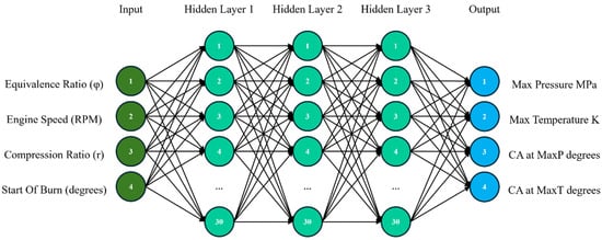
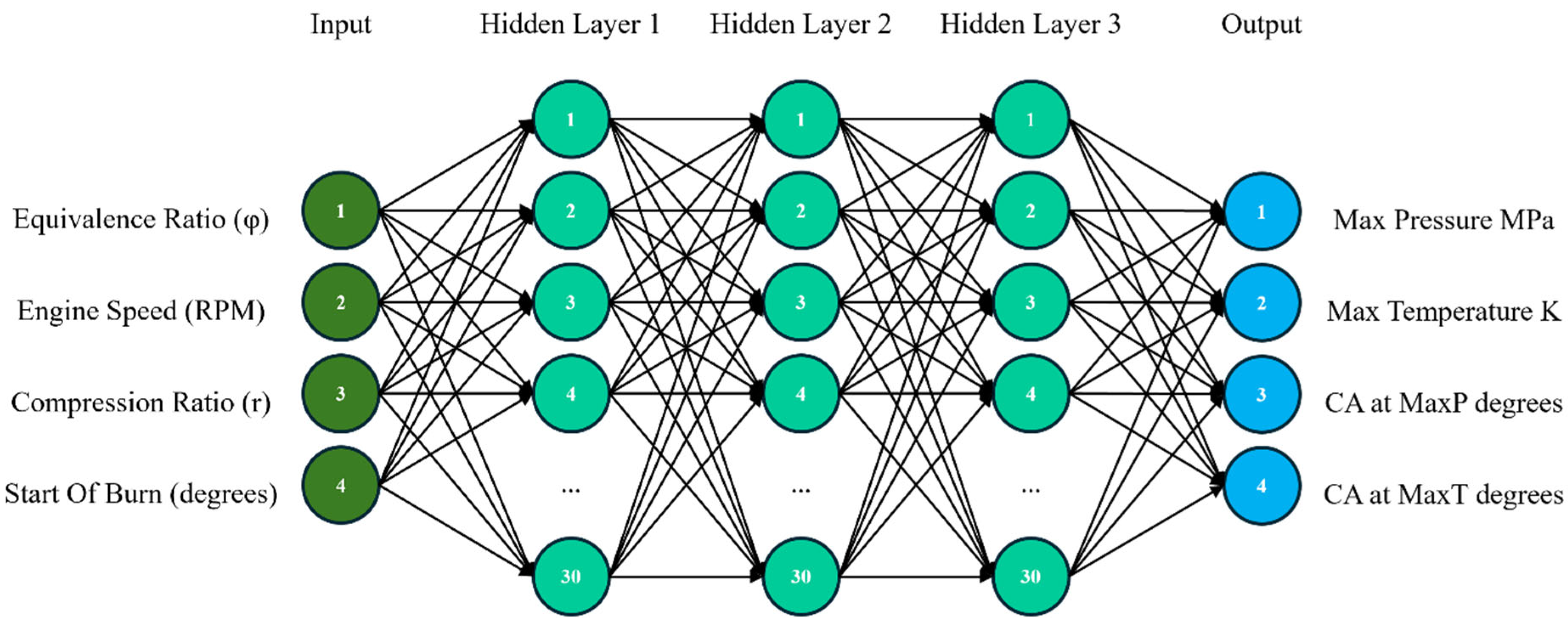
The network structure, illustrated in Figure 3, followed a standard multilayer perceptron architecture. It is important to note that Figure 3 presents a generalised schematic of the connectivity; the specific hidden-layer configurations (including layer depth and neuron counts) were treated as experimental variables and are detailed in the experimental matrix table below in the report. Hyperbolic tangent sigmoid activation functions were used for all hidden layers to capture nonlinear system dynamics, while a linear transfer function was applied at the output layer to allow for unbounded regression predictions. A custom weighting strategy was applied during the loss calculation where operating points featuring late combustion (start-of-burn > −5° ATDC) were assigned a higher importance factor of 3.0 to ensure adequate learning in these challenging regimes.

Figure 3. Schematic representation of the feed-forward artificial neural network architecture used for surrogate modelling. The diagram illustrates a general multilayer perceptron with fully connected hidden layers (tansig activation) and a linear output layer for regression prediction. Hidden-layer depth and neuron counts were varied during the architecture sweep (5-5 to 30-30-30). Although four physical inputs are illustrated, the start-of-burn angle was encoded using sine and cosine terms during training, resulting in a five-dimensional ANN input vector.

The specific training configuration is detailed in Table 3. The network weights and biases were optimised using the Levenberg–Marquardt backpropagation algorithm with mean squared error serving as the loss function. To ensure training stability, the optimisation was executed in controlled epoch chunks with intermediate checkpointing. A dual-seed strategy was employed to isolate the impact of network initialisation from data partitioning. A fixed global seed locked the random division of the dataset into training (70%), validation (15%) and testing (15%) subsets using fixed indices. A separate initialisation seed controlled the starting values of the network weights.

Table 3. Base ANN training configuration held constant across all architecture and seed sweep experiments.

Function/Step	Used in Script	Description
Data loading	readtable	Loads the cleaned dataset containing physical input parameters and regression targets.
Input selection	$T. \varphi$, T.RPM…	Selects physical engine and combustion parameters used as ANN inputs.
Angular conversion	$deg2rad$	Converts start-of-burn angle from degrees to radians prior to feature encoding.
Angular encoding	sin, cos	Encodes the start-of-burn angle using sine and cosine functions to preserve angular continuity.
Input matrix assembly	X_raw = […]	Constructs the 5-dimensional input matrix using   $\varphi$$, \mathrm{RPM}, r$$, \mathrm{s}\mathrm{i}\mathrm{n}\left(SoB\right)$$, \mathrm{and} \mathrm{c}\mathrm{o}\mathrm{s}\left(SoB\right)$.
Target selection	MaxPressure_MPa, CA_at_MaxP_deg, MaxTemperature_K, CA_at_MaxT_deg	Defines the 4 ANN outputs—peak in-cylinder pressure (MPa) and temperature (K), plus their crank-angle locations (deg aTDC)—for combustion performance prediction.
Data normalisation	$(x-\mu )/\sigma$	Applies Z-score standardisation using training-set statistics to prevent data leakage.
Base random seed	rng(100)	Sets a fixed base random seed to ensure identical data partitioning across all runs.
Weight initialisation	Sweeper-defined	Overrides the base seed with a specific seed_init to isolate the impact of weight initialisation.
ANN architecture control	Sweeper-defined	Controls the hidden-layer structure, exploring architectures from (5–5) to (30–30–30)].
ANN architecture def.	feedforwardnet	Instantiates a multilayer perceptron (MLP) using the specified hidden-layer architecture.
Data division	divideind	Uses fixed indices (70/15/15 split) derived from the base seed to ensure identical partitions.
Training algorithm	trainlm	Uses the Levenberg–Marquardt backpropagation algorithm for nonlinear regression.
Performance metric	mse	Uses mean squared error (L2 loss) as the loss function during ANN training.
Loss weighting	w_combined	Applies a 3.0x importance weight to operating points with late combustion (SoB > −5° aTDC).
Training execution	train	Trains the ANN using validation-based early stopping to prevent overfitting.
Model evaluation	Custom metrics	Computes regression performance metrics (R2, RMSE, MAE) on the test set.
Model saving	save	Stores trained networks, normalisation parameters, and metadata for reproducibility.

This rigorous separation of fixed training parameters and variable architectural definitions formed the basis of the experimental study. With the reproducible training framework established, the investigation proceeded to systematically evaluate how network capacity and initialisation stochastics influence model reliability, as described in the architecture–initialisation sweep design in the following section.

2.3.1. Angularly Continuous Input Encoding

The regression inputs are defined using an angularly continuous embedding of start-of-burn. Let ${\mathsf{\theta }}_{\mathrm{S}\mathrm{o}\mathrm{B},\mathrm{d}\mathrm{e}\mathrm{g}}$ denote start-of-burn in degrees and ${\mathsf{\theta }}_{\mathrm{S}\mathrm{o}\mathrm{B},\mathrm{r}\mathrm{a}\mathrm{d}}=(\pi /180){\mathsf{\theta }}_{\mathrm{S}\mathrm{o}\mathrm{B},\mathrm{d}\mathrm{e}\mathrm{g}}$. The raw input vector is

$${\mathrm{x}}_{\mathrm{r}\mathrm{a}\mathrm{w}}=\left[\begin{array}{c}\varphi \\ \mathrm{RPM}\\ r\\ \sin \left({\mathsf{\theta }}_{\mathrm{S}\mathrm{o}\mathrm{B},\mathrm{r}\mathrm{a}\mathrm{d}}\right)\\ \cos \left({\mathsf{\theta }}_{\mathrm{S}\mathrm{o}\mathrm{B},\mathrm{r}\mathrm{a}\mathrm{d}}\right)\end{array}\right]\in {\mathbb{R}}^5$$

(13)

where $\varphi$ is equivalence ratio, $\mathrm{R}\mathrm{P}\mathrm{M}$ is engine speed, and $r$ is compression ratio.

2.3.2. Train-Only Z-Score Normalisation

All inputs and targets are standardised using Z-score normalisation with statistics computed exclusively on the training subset. The normalised input vector is

$$\mathrm{x}=({\mathrm{x}}_{\mathrm{r}\mathrm{a}\mathrm{w}}-{\mu }_x)\oslash {\sigma }_x,$$

(14)

and the normalised target vector is

$$\mathrm{y}=({\mathrm{y}}_{\mathrm{r}\mathrm{a}\mathrm{w}}-{\mu }_y)\oslash {\sigma }_y,$$

(15)

where ${\mu }_x$ and ${\sigma }_x$ are the training-set mean and standard deviation vectors for inputs, ${\mu }_y$ and ${\sigma }_y$ are the training-set mean and standard deviation vectors for targets, and $\oslash$ denotes element-wise division.

2.3.3. Feedforward Network Mapping

A fully connected feedforward network with $L$ layers is used. Defining ${\mathrm{a}}^{\left(0\right)}=\mathrm{x}$, the hidden-layer transformation is

$${\mathrm{a}}^{\left(l\right)}=\mathrm{t}\mathrm{a}\mathrm{n}\mathrm{s}\mathrm{i}\mathrm{g}(\cdot )\left({\mathrm{W}}^{\left(l\right)}{\mathrm{a}}^{\left(l−1\right)}+{\mathrm{b}}^{\left(l\right)}\right),l=1,\dots ,L-1,$$

(16)

where ${\mathrm{W}}^{\left(l\right)}$ and ${\mathrm{b}}^{\left(l\right)}$ are the weight matrix and bias vector of layer $l$, and $\mathrm{t}\mathrm{a}\mathrm{n}\mathrm{s}\mathrm{i}\mathrm{g}(\cdot )$ is the MATLAB hyperbolic tangent sigmoid transfer function,

$$\mathrm{t}\mathrm{a}\mathrm{n}\mathrm{s}\mathrm{i}\mathrm{g}(n)={\displaystyle \frac{2}{1+e^{-2n}}}-1.$$

(17)

The output layer applies a linear transfer function,

$$\widehat{\mathrm{y}}={\mathrm{W}}^{\left(L\right)}{\mathrm{a}}^{\left(L−1\right)}+{\mathrm{b}}^{\left(L\right)},$$

(18)

where $\widehat{\mathrm{y}}\in {\mathbb{R}}^4$ contains the predicted peak pressure, crank angle at peak pressure, peak temperature, and crank angle at peak temperature.

2.3.4. Weighted Objective and Late-Combustion Emphasis

Training is performed using Levenberg–Marquardt backpropagation with a weighted mean squared error objective. Let $w_i$ denote the sample weight for operating point $i$. The loss is defined as

$$\mathcal{L}={\displaystyle \frac{1}{\sum _{i=1}^N{w}_i}}\sum _{i=1}^N{w}_i{\parallel {\mathrm{y}}_i-{\widehat{\mathrm{y}}}_i\parallel }_2^2,$$

(19)

where $N$ is the number of training samples. Operating points with late combustion are up-weighted such that $w_i=3$ for ${\theta }_{\mathrm{S}\mathrm{o}\mathrm{B},\mathrm{d}\mathrm{e}\mathrm{g}}>-5^{\circ }$, and $w_i=1$ otherwise. Validation samples are assigned unit weight.

2.3.5. Levenberg–Marquardt Update

The Levenberg–Marquardt parameter update can be expressed as

$${\theta }_{k+1}={\theta }_k-{\left({\mathrm{J}}^{\mathsf{T}}\mathrm{J}+\mu \mathrm{I}\right)}^{-1}{\mathrm{J}}^{\mathsf{T}}\mathrm{e},$$

(20)

where $\theta$ is the stacked vector of all network weights and biases, $\mathrm{e}$ is the residual vector, $\mathrm{J}$ is the Jacobian of residuals with respect to $\theta$, $\mu$ is the damping parameter, and $\mathrm{I}$ is the identity matrix.

2.4. Architecture–Initialisation Sweep Design

Using the fixed base training configuration described in Table 3, a structured sweep procedure was implemented to systematically investigate the influence of ANN architecture and stochastic weight initialisation on model performance. The sweep design, summarised in Table 4, explicitly separated invariant elements (data partitioning, preprocessing, and optimisation settings) from the experimental variables, ensuring that any observed performance differences could be attributed solely to architectural capacity or initialisation stability.

Table 4. ANN architecture and initialisation sweep configuration.

Function/Step	Used in Script	Description
Sweep controller	Sweep driver	Controls the execution of the architecture–seed sweep while invoking the base ANN training routine.
Base configuration	Fixed config	Inherits the fixed ANN training configuration defined in Table 3.
Data partition seed	seed_split = 100	Locks the train/validation/test data split across all sweep runs to ensure fair comparison.
Initialisation seed	seed_init	Varies the random seed used for ANN weight and bias initialisation; the full seed set is defined in Table 5.
Architecture definition	hiddenSizes	Specifies the ANN hidden-layer structure for each sweep case.
Architecture range	Sweep-defined	Explores two and three hidden-layer architectures; the full architecture set is detailed in Table 5.
Sweep execution	Nested loops	Iterates over all combinations of architecture and initialisation seed.
Training invocation	Base training routine	Trains one ANN model per sweep configuration.
Result logging	Structured outputs	Records performance metrics and training data for each sweep case.
Reproducibility control	Fixed split + config	Ensures performance differences arise solely from architecture and initialisation effects.

To identify a stable and well-performing model structure, the sweep explored a grid of network depths, neuron counts, and initialisation seeds. The experiment covered two-layer and three-layer architectures with widths ranging from 5 to 30 neurons, crossed with 10 distinct random initialisation seeds. This resulted in a total of 120 unique training runs, as detailed in the experimental matrix in Table 5.

Table 5. ANN architecture—seed experimental matrix.

Category	Values Evaluated
Initialisation seeds	1, 2, 3, 4, 5, 6, 7, 8, 9, 10
Two-layer architectures	5–5, 10–10, 15–15, 20–20, 25–25, 30–30
Three-layer architectures	5–5–5, 10–10–10, 15–15–15, 20–20–20, 25–25–25, 30–30–30
Total configurations	10 seeds × (6 two-layer + 6 three-layer) = 120 runs

All trained models were evaluated on the strictly held-out test subset (N = 53,178). To facilitate model selection, a multi-target ranking metric was defined as the average rank of the root mean squared error (RMSE) across all four outputs. This aggregate score ensured that the selected “best” model demonstrated balanced performance across pressure, temperature, and crank-angle targets, rather than optimising a single dominant variable.

3. Results

3.1. Overview of Architecture–Seed Sweep Performance

The experimental sweep described in Section 2.4 produced a total of 120 trained networks. As performance was computed independently for each of the four regression targets (maximum pressure, maximum temperature, crank angle at maximum pressure and crank angle at maximum temperature), this generated a total of 480 target-specific result entries (120 configurations × four outputs). Table 6 presents a representative subset of these results to illustrate the performance variation observed across different architectures and initialisation seeds.

Table 6. Representative sample of ANN performance metrics from the architecture–seed sweep.

Row No	Arch	Seed	Epoch	Target	Total Time_s	R2	RMSE	MAE	P95
1	10–10	1	500	CA_MaxP_deg	130.28	0.9989	0.3557	0.1345	0.3193
2	10–10	1	500	CA_MaxT_deg	130.28	0.9997	0.1707	0.1249	0.3257
3	10–10	1	500	MaxP_MPa	130.28	0.9998	0.0334	0.0250	0.0684
4	10–10	1	500	MaxT_K	130.28	0.9996	4.7603	3.7212	9.3436
129	15–15–15	3	241	CA_MaxP_deg	311.29	0.9999	0.0813	0.0168	0.0414
130	15–15–15	3	241	CA_MaxT_deg	311.29	1.0000	0.0261	0.0178	0.0509
131	15–15–15	3	241	MaxP_MPa	311.29	1.0000	0.0048	0.0035	0.0095
132	15–15–15	3	241	MaxT_K	311.29	1.0000	0.5520	0.4139	1.0940
305	25–25–25	7	141	CA_MaxP_deg	1725.68	1.0000	0.0413	0.0115	0.0288
306	25–25–25	7	141	CA_MaxT_deg	1725.68	1.0000	0.0162	0.0118	0.0309
307	25–25–25	7	141	MaxP_MPa	1725.68	1.0000	0.0029	0.0021	0.0055
308	25–25–25	7	141	MaxT_K	1725.68	1.0000	0.4139	0.3068	0.8155
477	5–5–5	10	500	CA_MaxP_deg	76.82	0.9907	1.0509	0.3009	0.7217
478	5–5–5	10	500	CA_MaxT_deg	76.82	0.9983	0.4287	0.3079	0.8715
479	5–5–5	10	500	MaxP_MPa	76.82	0.9988	0.0793	0.0611	0.1490
480	5–5–5	10	500	MaxT_K	76.82	0.9971	13.4500	10.4381	24.8650

Analysis of the complete experimental set reveals distinct quantitative trends regarding network capacity and computational cost. First, predictive accuracy improved rapidly as network width increased from small to medium capacity. The mean test RMSE across all targets dropped from approximately 4.39 for the 5–5 architecture to 0.52 for the 15–15 architecture. However, extending the width further yielded diminishing returns; the 25–25 architecture achieved a mean RMSE of 0.30 but required an average training time of 1169 s, which is more than double the 545 s required for the 20–20 configuration (mean RMSE 0.33).

Second, increasing network depth did not universally guarantee improved efficiency. While three-layer architectures generally achieved lower absolute errors, the computational penalty was severe. For example, the 20–20–20 architecture achieved a mean RMSE of 0.23 compared to 0.33 for the 20–20 model, but the mean training duration increased from 545 s to 1276 s. This indicates that while deeper networks can extract marginally better features, the underlying thermodynamic mapping is sufficiently smooth to be approximated well by wider two-layer structures at a lower computational cost.

Third, the stability of the training process was heavily dependent on the initialisation seed for smaller networks. The 5–5 architecture exhibited a standard deviation in MaxT RMSE of approximately 1.01 K across the ten seeds, whereas the 25–25 architecture showed a standard deviation of only 0.21 K. This five-fold reduction in variability confirms that larger architectures are less sensitive to the stochastic starting point of the optimisation, reliably converging to a high-quality solution.

It is also important to note that performance metrics are reported to four decimal places. Consequently, very high-performing configurations may exhibit coefficient of determination (R2) values of 1.0000 in the tables due to rounding, even though finite residual errors persist.

3.2. Selection of Representative Configurations

To isolate the impact of architectural capacity from stochastic noise, a structured selection procedure was applied to the 120 trained networks, with the specific aim of identifying performance bounds for detailed phenomenological analysis. Rather than relying on a single aggregate metric, which can obscure trade-offs between competing regression targets, the selection of representative “high-capacity” and “low-capacity” models was driven by a multi-objective analysis of consistency and balance across the full thermodynamic state vector. The resulting configurations, designated as CS1 and CS2, define the operational envelope of the study and are summarised in Table 7.

Table 7. Selected highest and lowest capacity ANN configurations with convergence and multi-target performance summary.

Model	Architecture	Seed	Epochs	Total Time (s)	RMSE MaxP (MPa)	RMSE CA@MaxP (deg)	RMSE MaxT (K)	RMSE CA@MaxT (deg)
CS2 (High capacity)	25–25–25	6	161	1974.831	0.0025	0.0405	0.3645	0.0142
CS1 (Low capacity)	5–5	8	500	52.3796	0.1166	0.8189	17.5998	0.6017

To provide a quantitative definition of representational capacity, the total number of trainable parameters in a fully connected feedforward network is given by

$$N_{params}=\sum _{l=1}^L(n_{l-1}{n}_l+n_l)$$

(21)

where $n_l$ denotes the number of neurons in layer $l$, and the summation includes both weights and biases across all layers.

For the 5–5 configuration (CS1), the total number of trainable parameters is

$$(5\times 5+5)+(5\times 5+5)+(5\times 4+4)=84$$

(22)

For the 25–25–25 configuration (CS2), the total number of trainable parameters is

$$(5\times 25+25)+(25\times 25+25)+(25\times 25+25)+(25\times 4+4)=1554$$

(23)

Thus, CS2 contains 18.5 times more trainable parameters than CS1, establishing a precise quantitative distinction between low-capacity and high-capacity architectures.

The configuration designated as CS2 (25–25–25 architecture with Seed 6) was selected as the representative high-performance model. While several large-capacity configurations achieved near-perfect R2 values, Seed 6 was distinguished by its exceptional balance across all four outputs. Unlike other top-ranking candidates (e.g., Seeds 1 and 7) which occasionally minimised pressure error at the expense of temperature precision, Seed 6 demonstrated a uniform minimisation of residual error across the entire output vector. It converged to a stable validation minimum at epoch 161 (training time is 1974.8 s) and achieved validation RMSE values of 0.0025 MPa (MaxP), 0.3645 K (MaxT), 0.0405° (CA@MaxP), and 0.0142° (CA@MaxT). This uniform fidelity makes it the most scientifically robust candidate for generative evaluation.

Conversely, the configuration designated as CS1 (5–5 architecture with Seed 8) was identified as the representative baseline for capacity limitation. Just as CS2 was selected for its consistent superiority, CS1 was selected for its consistent failure to resolve the system dynamics across all targets. Despite being trained for the maximum allowance of 500 epochs (training time is 52.4 s), it failed to converge to a low-error state, yielding RMSE values orders of magnitude higher than the optimal configuration: 0.1166 MPa (MaxP), 17.5998 K (MaxT), 0.8189° (CA@MaxP), and 0.6017° (CA@MaxT).

The selection of these two configurations provides a rigorous phenomenological contrast. CS2 represents a converged, high-fidelity approximation of the physics-based manifold, while CS1 represents a structurally constrained regression that captures global trends but fails to resolve local nonlinearities. The following sections analyse the operational consequences of this capacity gap.

The RMSE values in Table 7 correspond to validation-set performance at the epoch of convergence; final generalisation metrics on the held-out test set are reported separately in predictive error metrics table, below.

3.3. Case Study Definition

The Results section presents a focused comparison between the lowest- and highest-ranked ANN configurations identified in the architecture–seed sweep. These two models define the observed performance bounds and are analysed to characterise how structural differences translate into surrogate behaviour.

CS1 corresponds to the lowest-ranked configuration (5–5, Seed 8), exhibiting limited representational capacity and reduced predictive performance. CS2 corresponds to the highest-ranked configuration (25–25–25, Seed 6), demonstrating substantially stronger predictive capability and stable optimisation behaviour.

Unless stated otherwise, all metrics reported in this section correspond to the held-out test dataset (N = 53,178 per regression target), ensuring that comparisons reflect generalisation performance rather than training artefacts.

3.4. Training Behaviour and Convergence

The optimisation histories reveal a pronounced divergence in convergence dynamics Fbetween the two configurations. CS1 exhibited rapid initial loss reduction during the first about 10–15 epochs, followed by an early plateau. Despite training to the maximum permitted 500 epochs, no distinct validation minimum was established. Training and validation curves remained closely coupled and flattened at a comparatively elevated MSE level, indicating that extended optimisation did not yield further functional refinement. In contrast, CS2 demonstrated sustained loss reduction beyond the initial transient phase and terminated via validation-based early stopping at epoch 161. The terminal validation MSE of CS2 was more than one order of magnitude lower than that of CS1, and the separation between training and validation loss remained minimal throughout optimisation, consistent with stable convergence and effective generalisation control.

This divergence can be summarised as follows:

• CS1 (5–5, Seed 8): Early loss reduction followed by premature plateau; no stable validation minimum within 500 epochs; convergence limited by structural expressiveness and initialisation trajectory.
• CS2 (25–25–25, Seed 6): Progressive convergence; validation-triggered stopping at epoch 161; substantially lower terminal MSE and stable generalisation behaviour.

The increase in representational capacity was accompanied by a substantial rise in computational cost. CS1 (5–5, Seed 8) completed 500 epochs in approximately 52.4 s, whereas CS2 (25–25–25, Seed 6) required approximately 1974.8 s (33 min) despite terminating at epoch 161 via early stopping. On a per-epoch basis, CS2 required approximately 12.3 s compared with approximately 0.10 s for CS1, reflecting the increased parameter count and associated optimisation overhead. Thus, while CS2 achieved markedly improved convergence quality and lower terminal loss, this gain was accompanied by a significant computational cost increase.

These results indicate that convergence stability and predictive fidelity improve with increased representational capacity, but at the expense of training efficiency. The implications of this trade-off for predictive accuracy and error distribution behaviour are examined in the following section.

3.5. Overall Predictive Accuracy

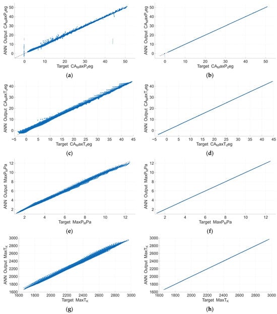
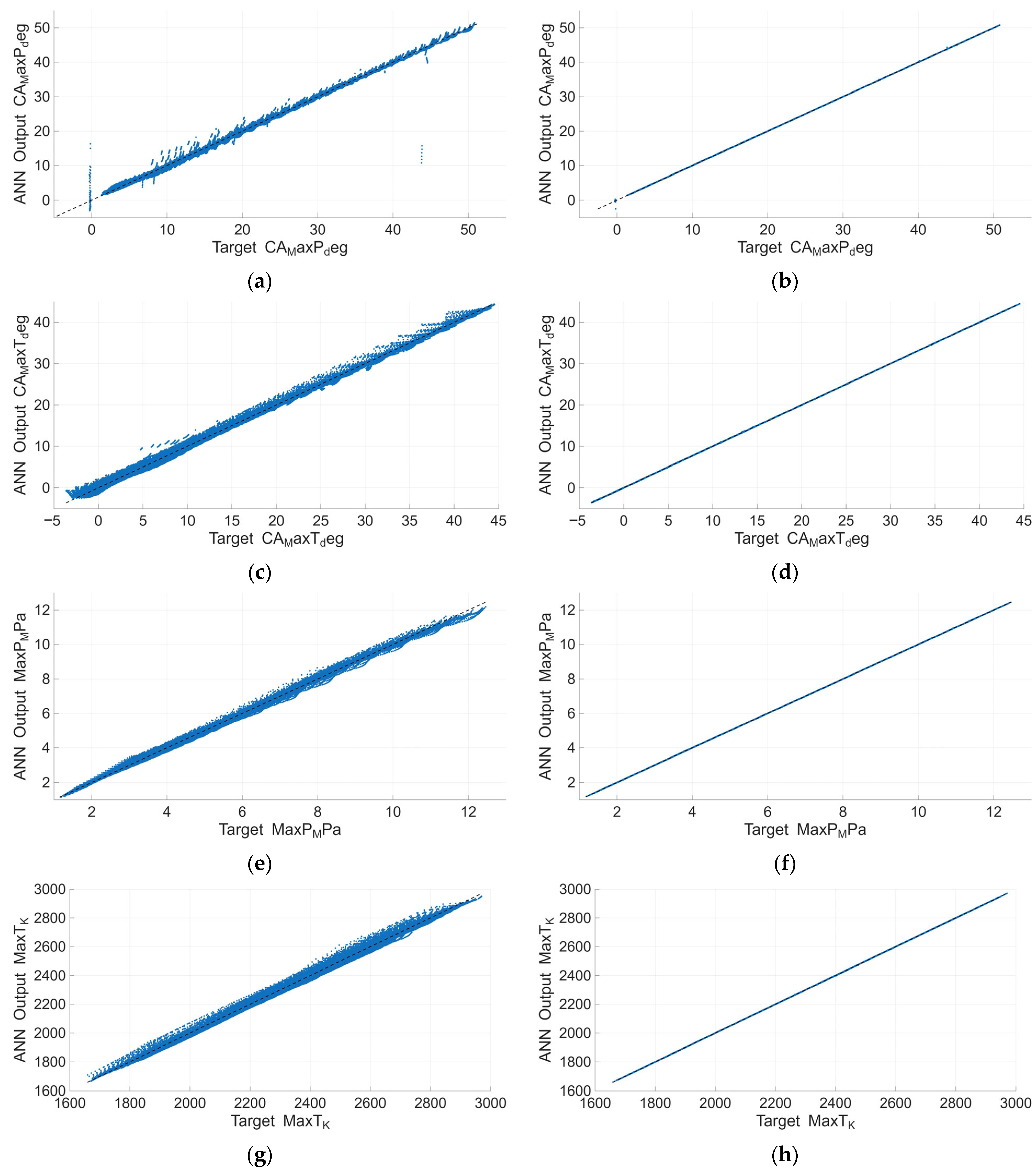
Figure 4 demonstrates that the convergence differences translate directly into predictive fidelity. CS2 exhibits a tight clustering around the unity line for all outputs, indicating that the learned mapping reproduces both trend and magnitude with minimal dispersion. CS1 shows visibly increased scatter and localised systematic deviation, most evident towards the extremes of the target ranges. This behaviour is consistent with capacity-limited regression, where the network captures global trends (hence high correlation) but fails to resolve finer nonlinear structure across the operating envelope.

Figure 4. Parity plots comparing ANN predictions against reference (physics-generated) targets for CS1 and CS2. (a,b) CA@MaxP (CS1, CS2), (c,d) CA@MaxT (CS1, CS2), (e,f) MaxP (CS1, CS2), (g,h) MaxT (CS1, CS2). The solid line indicates the unity (perfect agreement) relationship.

3.6. Quantitative Error Metrics

Table 8 quantifies the performance separation between the two surrogates. Although both configurations achieve high coefficients of determination (R² > 0.99), CS2 reduces absolute errors by approximately 30–50× relative to CS1 across all targets. This distinction is particularly consequential for crank-angle phasing metrics, where sub-degree errors can materially alter inferred combustion timing sensitivity. Importantly, CS2 achieves this improvement with near-zero bias across all targets, indicating that accuracy gains arise from improved functional approximation rather than cancellation of opposing errors. The persistence of large absolute errors in CS1 despite similarly high R² values further demonstrates that the underlying regression task is non-trivial and that correlation-based metrics alone are insufficient to characterise surrogate quality.

Table 8. Predictive error metrics for CS1 and CS2 on the held-out test set (N = 53,178 per target). RMSE and MAE quantify absolute error magnitude; bias is the mean signed error (prediction—reference). MinErr and MaxErr report extrema of the signed error distribution. All crank-angle targets are in degrees and MaxP is in MPa.

CS1	Target	Max Pressure (MPa)	Crank Angle at Max Pressure (deg)	Max Temperature (K)	Crank Angle at Max Temperature (deg)
	N	53,178.0000	53,178.0000	53,178.0000	53,178.0000
	RMSE	0.1161	0.6420	17.6838	0.6057
	MAE	0.0887	0.3942	13.4609	0.4656
	Bias	−0.0033	−0.0231	−0.1842	0.0205
	R2	0.9974	0.9965	0.9950	0.9965
	R	0.9987	0.9983	0.9975	0.9983
	MinErr	−0.5818	−33.0145	−51.7983	−1.9776
	MaxErr	0.6743	16.4960	114.1144	4.6726
	StdErr	0.1161	0.6416	17.6830	0.6054
CS2	Target	Max Pressure (MPa)	Crank Angle at Max Pressure (deg)	Max Temperature (K)	Crank Angle at Max Temperature (deg)
	N	53,178.0000	53,178.0000	53,178.0000	53,178.0000
	RMSE	0.0025	0.0208	0.3568	0.0141
	MAE	0.0019	0.0106	0.2706	0.0102
	Bias	0.0000	−0.0003	0.0033	−0.0001
	R2	1.0000	1.0000	1.0000	1.0000
	R	1.0000	1.0000	1.0000	1.0000
	MinErr	−0.0205	−2.3730	−3.1383	−0.1724
	MaxErr	0.0330	0.5692	3.9468	0.2243
	StdErr	0.0025	0.0208	0.3568	0.0141

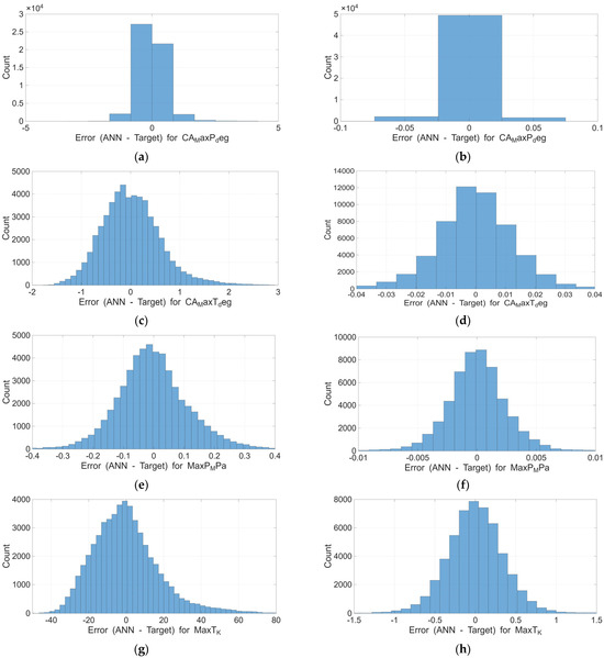
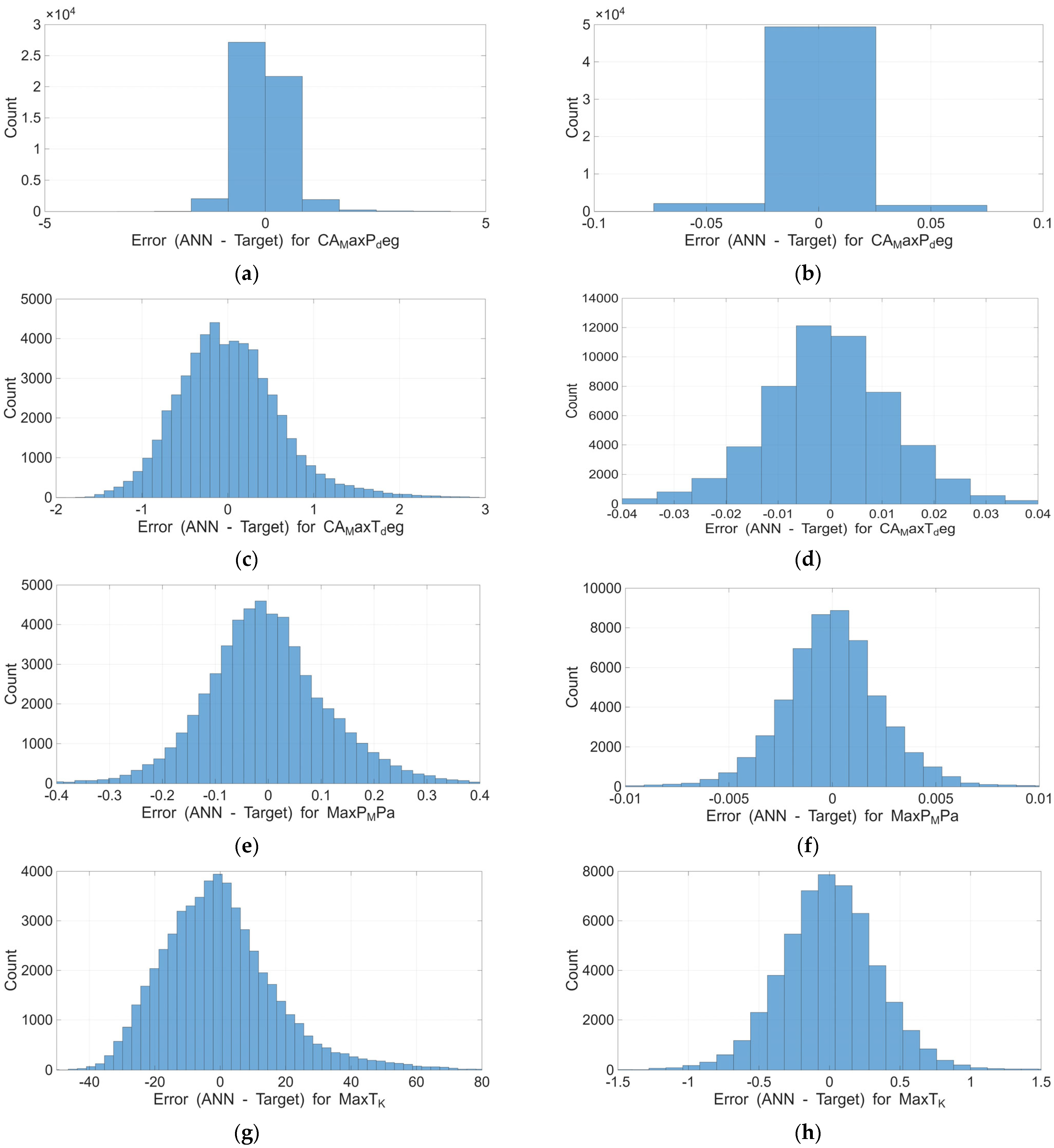
While Table 8 summarises mean error metrics, distribution-level behaviour reveals additional structural differences between architectures. For the low-capacity configuration (CS1), root mean squared error values were 0.1161 MPa for peak pressure and 17.6838 K for peak temperature. For the high-capacity configuration (CS2), corresponding errors were reduced to 0.0025 MPa and 0.3568 K, respectively.

These results correspond to reduction factors of approximately 46× for peak pressure and 50× for peak temperature. However, mean error metrics alone do not fully characterise surrogate robustness.

Inspection of the residual distributions shows substantial differences in tail behaviour. Extreme-case peak temperature deviations reached 114.1144 K in the low-capacity configuration, whereas the maximum deviation in the high-capacity model was limited to 3.9468 K. Similarly, peak pressure deviations were reduced from 0.6743 MPa in CS1 to 0.0330 MPa in CS2.

Although both configurations achieved coefficients of determination exceeding 0.99, the low-capacity architecture exhibited heavy-tailed residual distributions and regime-dependent error amplification. In contrast, the high-capacity model produced tightly clustered residuals with substantially reduced tail behaviour. High coefficients of determination do not guarantee engineering reliability in nonlinear thermodynamic systems; correlation-based metrics alone cannot capture tail behaviour or extreme-case risk.

3.7. Error Distribution Characteristics

Residual distributions for CS2 are narrow and approximately symmetric about zero for all targets, consistent with the low RMSE and MAE values reported in Table 8. CS1 exhibits substantially broader distributions with heavier tails, implying a higher probability of large errors even when mean correlation remains strong. The contrast between CS1 and CS2 therefore highlights that aggregate fit metrics alone can mask materially different risk profiles for outlier prediction error (Figure 5).

Figure 5. Residual (prediction–reference) histograms for CS1 and CS2. (a,b) CA@MaxP (CS1, CS2), (c,d) CA@MaxT (CS1, CS2), (e,f) MaxP (CS1, CS2), (g,h) MaxT (CS1, CS2).

3.8. Dependence of Error on Operating Conditions

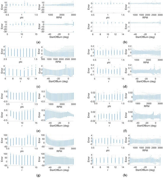
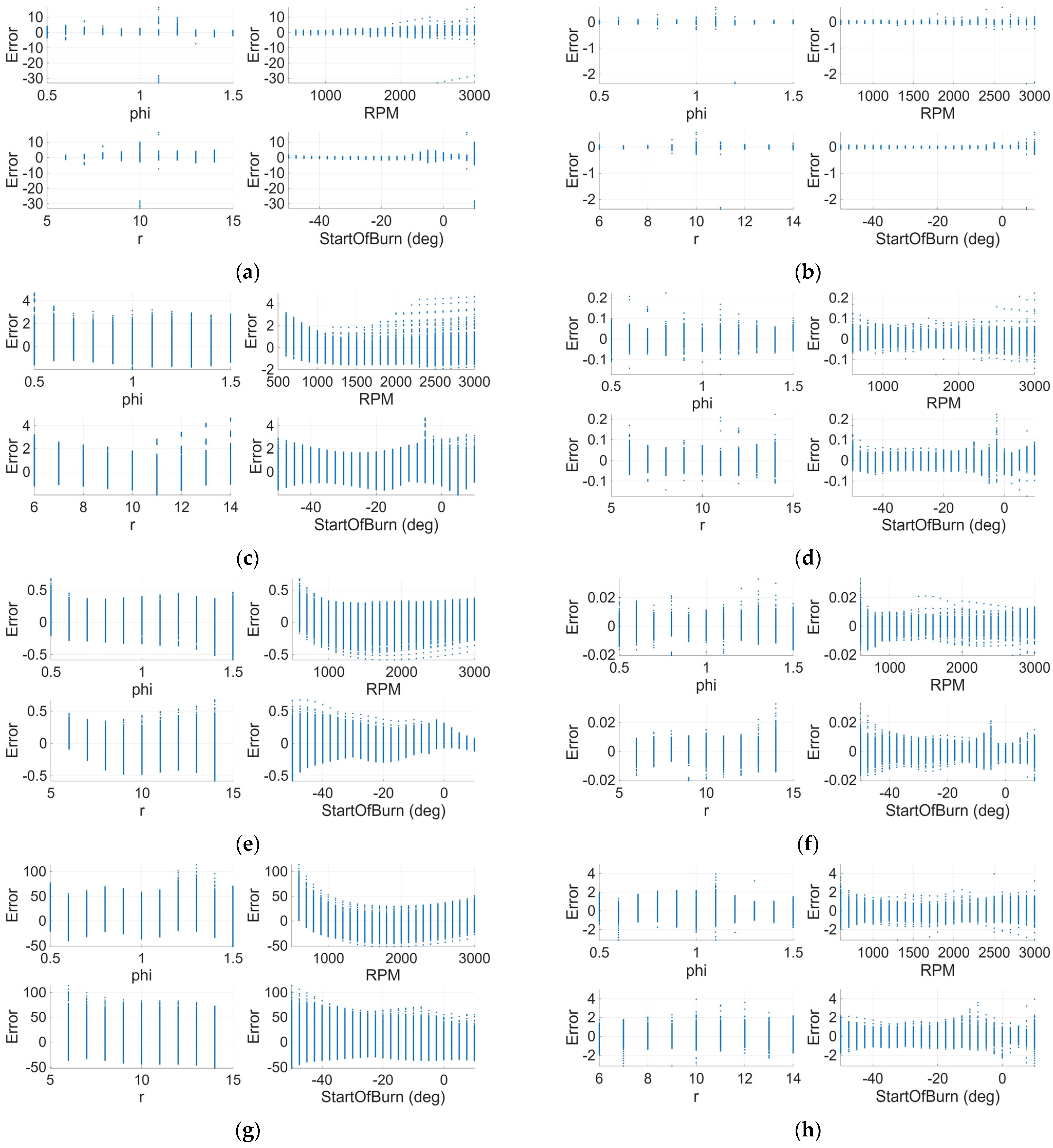
Figure 6 assesses whether errors remain approximately exchangeable across the operating envelope or become regime-dependent. CS2 residuals show weak structure and limited dependence on operating inputs, indicating robust generalisation with respect to the sampled operating envelope defined by the physics-generated dataset. In contrast, CS1 exhibits pronounced, structured residual patterns that correlate with specific operating regimes, consistent with capacity-limited learning where the surrogate approximates well in some regions but under-resolves nonlinear behaviour elsewhere. Such a regime-dependent error structure is undesirable for surrogate deployment, as it can bias downstream sensitivity studies and generative sampling towards systematically distorted regions of the domain.

Figure 6. Residuals (prediction–reference) as a function of input parameters for CS1 and CS2. (a,b) CA@MaxP (CS1, CS2), (c,d) CA@MaxT (CS1, CS2), (e,f) MaxP (CS1, CS2), (g,h) MaxT (CS1, CS2).

3.9. Base vs. Generated Data Consistency

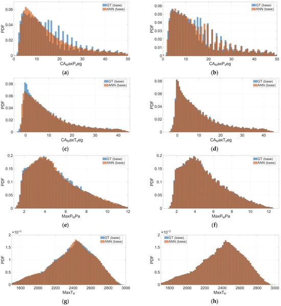
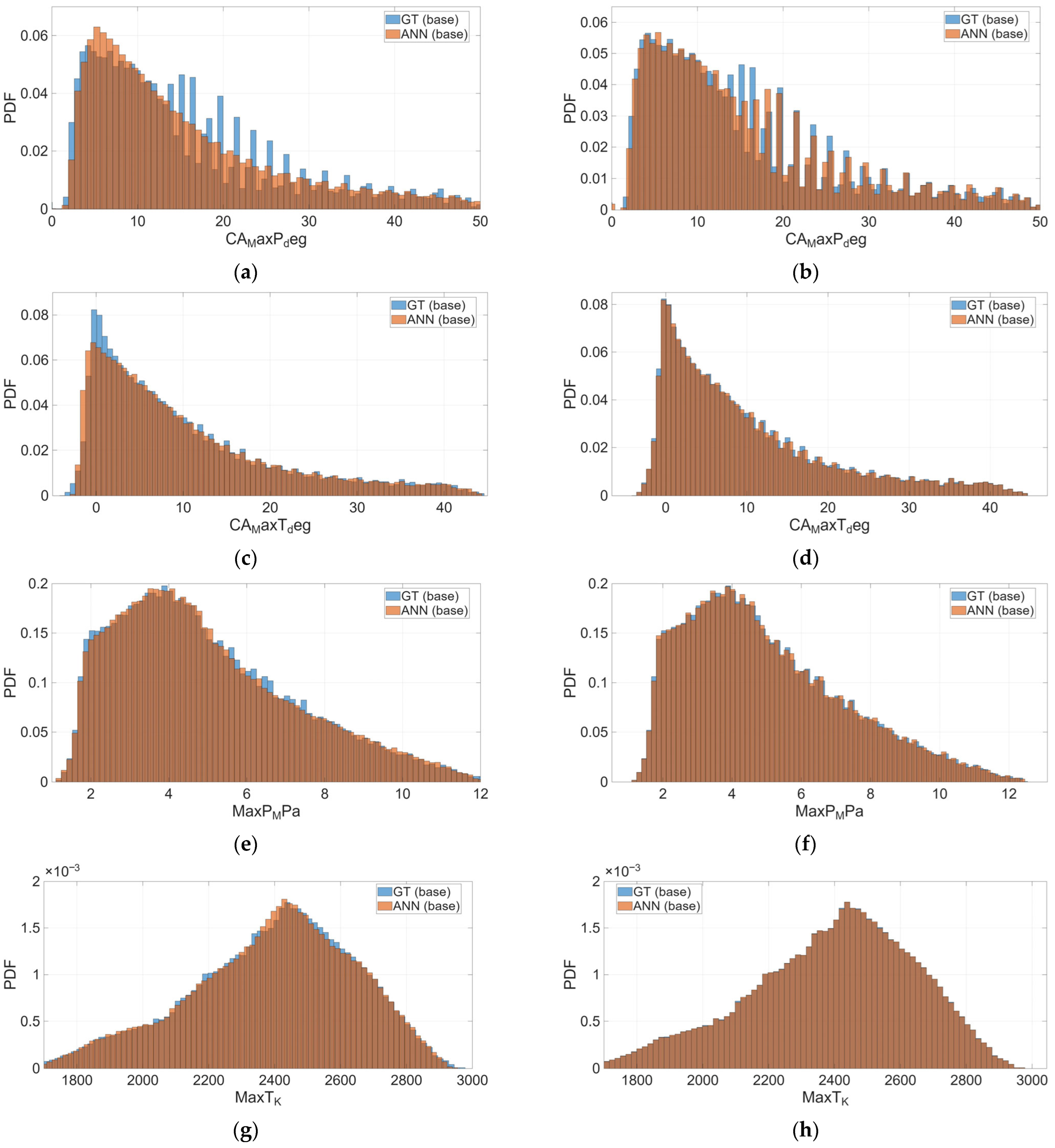
Figure 7 evaluates distributional fidelity under ANN-generated sampling. CS2 reproduces the base dataset PDFs closely across all targets, indicating statistical consistency with the physics-generated reference dataset. CS1 introduces visible distortion, particularly in the tails, implying that low-capacity surrogates may generate statistically biassed samples even when conventional regression metrics appear strong. This result is important for dataset augmentation workflows, where preservation of tail behaviour is often critical for robust surrogate training and uncertainty-aware inference.

Figure 7. Probability density function overlays comparing base (physics-generated) and ANN-generated outputs for CS1 and CS2. (a,b) CA@MaxP (CS1, CS2), (c,d) CA@MaxT (CS1, CS2), (e,f) MaxP (CS1, CS2), (g,h) MaxT (CS1, CS2).

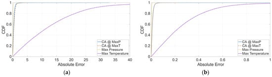
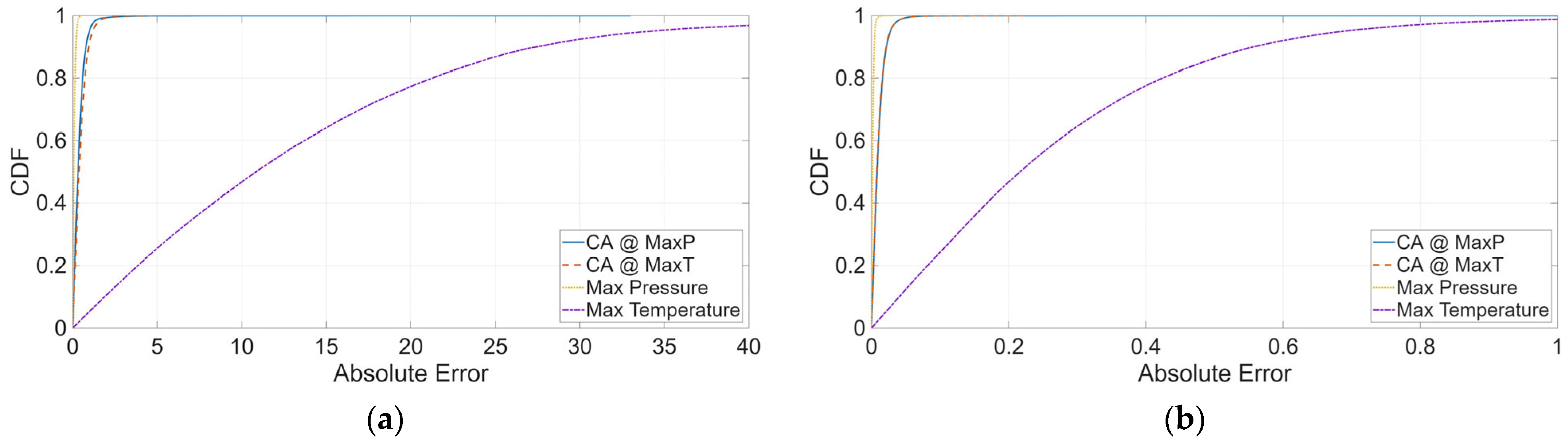
While Figure 7 compared the statistical distributions of base and ANN-generated outputs, it does not characterise how prediction error is distributed across the dataset. To evaluate error behaviour across the full quantile range, Figure 8 presents cumulative distribution functions (CDFs) of the absolute prediction error for all four regression targets under CS1 and CS2. This representation enables assessment not only of central tendency, but also of dispersion and extreme-value behaviour.

Figure 8. Cumulative distribution functions (CDFs) of absolute prediction error for (a) CS1 and (b) CS2, shown for CA@MaxP, CA@MaxT, max pressure, and max temperature.

Figure 8 reveals a clear and consistent separation between the two configurations across all targets. For CA@MaxP, approximately 95% of CS2 predictions fall within roughly 0.05° absolute error, whereas CS1 requires approximately 2–3° to reach comparable cumulative probability. A similar pattern is observed for CA@MaxT; 95% of CS2 samples remain below approximately 0.05°, while CS1 approaches approximately 1–1.5° at the same percentile level. For MaxP, the 95th percentile error in CS2 is below approximately 0.006 MPa, whereas CS1 approaches approximately 0.20 MPa. The largest divergence is observed for MaxT. Under CS2, approximately 95% of samples lie within roughly 1 K, and the distribution saturates below approximately 4 K. In contrast, CS1 requires on the order of 40–50 K to achieve 95% coverage, with the upper tail extending beyond 110 K. These results demonstrate that the improvement in CS2 is distribution-wide rather than confined to mean error reduction. Both central dispersion and extreme-value risk are substantially compressed relative to the low-capacity configuration.

3.10. Geometric Consistency of the Solution Space

This section examines whether data-driven model sampling preserves the geometric structure of the physics-generated dataset. While earlier subsections assessed convergence, pointwise accuracy, residual behaviour and statistical consistency, the present analysis focuses on structural fidelity in reduced-order space. The aim is to determine whether generated outputs remain embedded within the dominant solution structure defined by the reference dataset.

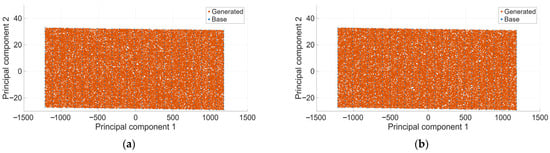
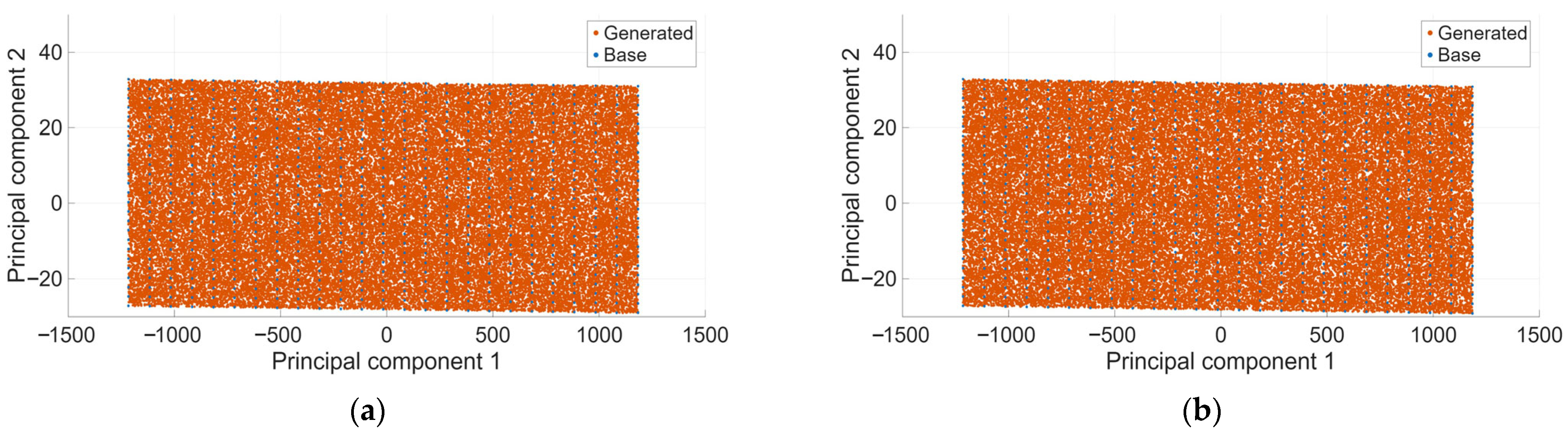
Figure 9 presents two-dimensional principal component projections of the base dataset and ANN-generated samples for CS1 and CS2. Principal component analysis was applied to the four-dimensional output space comprising maximum pressure, crank angle at maximum pressure, maximum temperature, and crank angle at maximum temperature. The first two principal components capture the dominant variance directions and provide a compact representation of the dataset geometry.

Figure 9. Two-dimensional principal component analysis (PCA) projections of base (physics-generated) and ANN-generated samples. (a) CS1 and (b) CS2.

For both configurations, the generated samples broadly overlap with the base dataset in principal component space. No large-scale rotation, separation or fragmentation of the point cloud is observed. This indicates that even the capacity-limited CS1 model captures the primary thermodynamic trends governing the system. The dominant low-dimensional structure defined by the correlated combustion outputs is therefore preserved under data-driven sampling. Minor visual differences are evident, with CS1 exhibiting slightly increased dispersion relative to the reference cloud, whereas CS2 remains tightly aligned. These differences, however, are subtle, reflecting the fact that both models reproduce the global variance structure of the dataset.

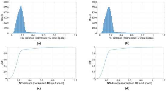
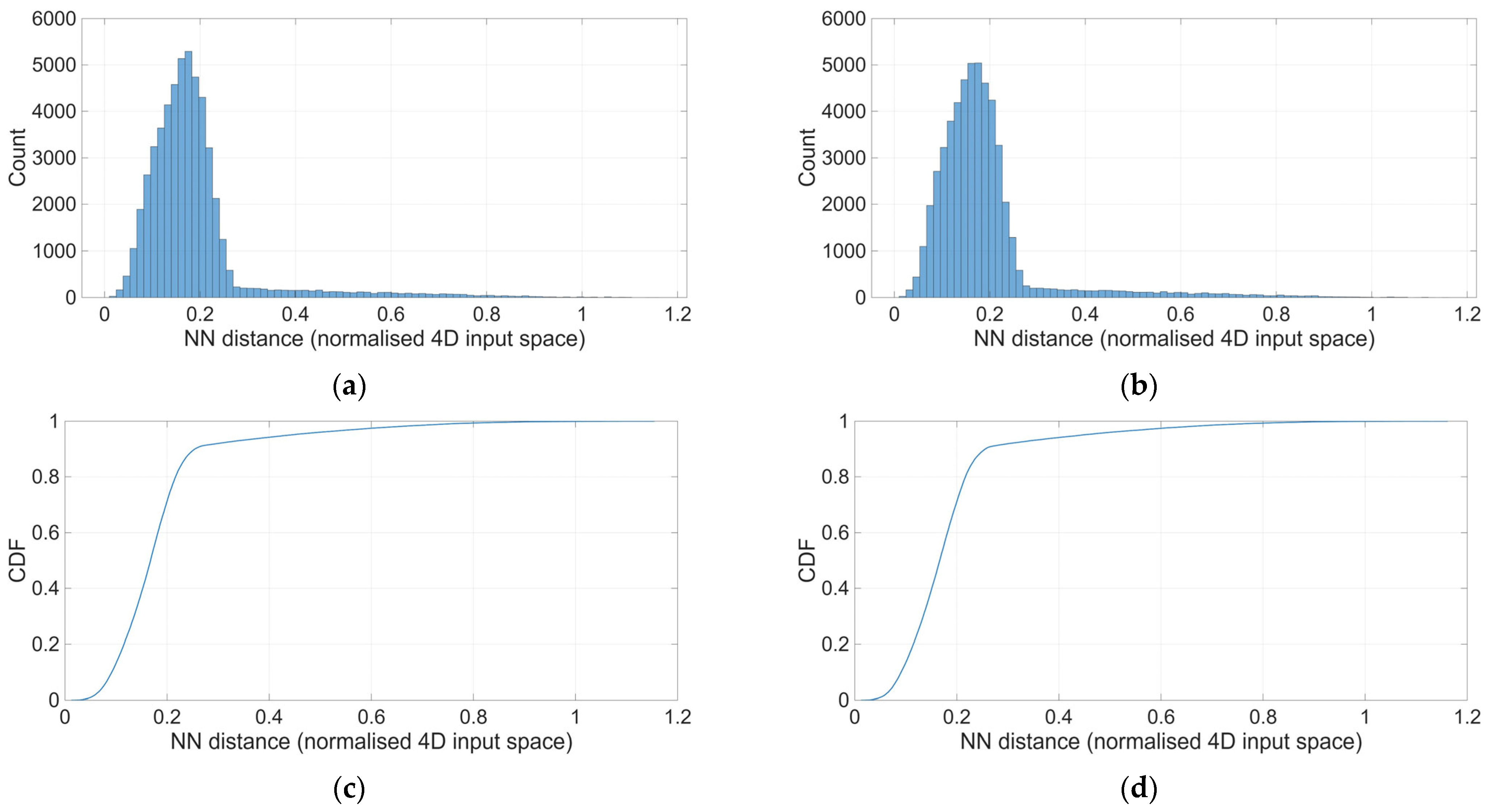
To assess geometric fidelity beyond visual inspection, nearest-neighbour distance statistics are shown in Figure 10. For each generated sample, the distance to the closest reference point was computed in the original feature space. This metric quantifies how closely generated outputs remain embedded within the base data structure.

Figure 10. Nearest-neighbour distance statistics between base and ANN-generated samples. (a,c) CS1 results and (b,d) CS2 results, showing complementary distributional and cumulative distance measures. A = CS1 NN distance histogram, C = CS1 NN distance CDF.

CS2 produces systematically smaller nearest-neighbour distances across the distribution, with a compressed upper tail. CS1 exhibits broader dispersion and a heavier tail, indicating a greater proportion of samples that deviate from the reference manifold. These deviations are not sufficiently large to disrupt global principal component alignment, but they represent local geometric distortion that becomes relevant in generative applications.

It is therefore noteworthy that, despite substantial differences in absolute error magnitude, tail behaviour and nearest-neighbour statistics, both CS1 and CS2 reproduce the dominant low-dimensional structure of the physics-generated dataset in principal component space. This suggests that the underlying dataset defines a geometrically coherent and smoothly varying mapping between inputs and outputs that is amenable to data-driven approximation. The distinction between the two configurations lies not in global structural recognition, but in the resolution of fine-scale nonlinear behaviour and extreme-value fidelity. CS2 preserves both the overall manifold and its local neighbourhood structure, whereas CS1 captures the former but partially degrades the latter.

These geometric findings complement the statistical and residual analyses presented earlier. Their implications for model reliability and generative robustness are discussed in the following section.

3.11. Summary of Comparative Findings

Table 9 is intended as a qualitative synthesis of the diagnostic evidence presented in Section 3.2, Section 3.3, Section 3.4, Section 3.5, Section 3.6, Section 3.7 and Section 3.8 rather than a replacement for the quantitative metrics reported in Table 8.

Table 9. Qualitative synthesis of surrogate performance differences between CS1 (worst-ranked) and CS2 (highest-ranked), integrating convergence behaviour, pointwise accuracy, regime dependence, and distributional/geometric fidelity.

Aspect	CS1	CS2
Convergence	Reached max epochs without stable minimum	Stable convergence before epoch limit
RMSE (all targets)	Higher	Lower
MAE (all targets)	Higher	Lower
R2 consistency	Variable	Consistently high
Error dependence on inputs	Structured, regime-dependent	Weak/negligible
Output distribution fidelity	Distorted PDFs	Preserved PDFs
Manifold distance (mean)	Larger	Smaller
Manifold consistency relative to base dataset	Reduced	Strong

Table 9 consolidates the comparative evidence from convergence histories, pointwise error metrics, residual diagnostics, and distributional/geometric analyses. The results consistently indicate that increased representational capacity enables stable convergence, reduces both mean error and tail risk, weakens regime-dependent error structure, and better preserves the base dataset manifold under generative sampling.

4. Discussion

The results demonstrate a clear and quantifiable separation between low-capacity and high-capacity data-driven neural network configurations. Across all four regression targets, the selected high-capacity model CS2 (25–25–25, Seed 6) achieves reductions in RMSE of approximately 30 to 50 times relative to the low-capacity configuration CS1 (5–5, Seed 8), as shown in Table 8. For maximum temperature, RMSE decreases from 17.68 K in CS1 to 0.36 K in CS2. For crank angle at maximum pressure, RMSE reduces from 0.64° to 0.02°. Maximum pressure RMSE decreases from 0.116 MPa to 0.0025 MPa. These reductions occur despite both configurations reporting R² values exceeding 0.99. The evidence therefore confirms that correlation metrics alone are insufficient to evaluate reliability in nonlinear thermodynamic mappings.

The architecture–initialisation sweep, summarised in Table 4, Table 5 and Table 6, clarifies how these differences emerge. Increasing width from 5 to 5 to 15–15 reduces mean RMSE across targets from approximately 4.39 to 0.52, with diminishing returns thereafter. The 25–25 configuration achieves mean RMSE near 0.30, while the three-layer 25–25–25 configuration produces further refinement. However, this improvement carries computational cost. CS1 completed 500 epochs in 52.4 s, whereas CS2 required approximately 1974.8 s to converge at epoch 161. On a per-epoch basis, the larger network required roughly two orders of magnitude greater computational effort. The thermodynamic mapping appears globally smooth in its dominant variance structure, yet exhibits sufficient local curvature to require increased representational capacity when high-resolution approximation is desired.

Initialisation seed plays a measurable role, particularly for small networks. The 5–5 architecture exhibits a standard deviation in MaxT RMSE of approximately 1.01 K across ten seeds, whereas the 25–25 architecture shows only 0.21 K variability. Larger architectures therefore demonstrate reduced sensitivity to stochastic initialisation and converge more consistently to low-error solutions. This stability is evident in Table 7, where CS2 converges via validation-based early stopping at epoch 161, while CS1 fails to establish a clear validation minimum even after 500 epochs. The distinction is structural rather than procedural; extended training does not compensate for limited representational capacity.

Figure 4 and Figure 5 translate these numerical differences into distributional behaviour. Parity plots show that CS2 predictions align tightly with the unity line across the full operating envelope, whereas CS1 displays visibly larger dispersion, particularly near target extremes. Residual histograms reveal heavy tails in CS1, with maximum temperature errors exceeding 110 K in extreme cases, compared with approximately 4 K in CS2. The cumulative error curves in Figure 8 further emphasise this separation. Approximately 95 percent of CS2 temperature predictions fall within 1 K, while CS1 requires tolerances near 40–50 K to achieve similar coverage. The improvement is therefore not confined to mean error reduction but extends across the entire error distribution.

Error structure with respect to operating conditions, shown in Figure 6, provides additional insight. CS2 residuals remain weakly structured across equivalence ratio, compression ratio and engine speed. CS1, by contrast, exhibits regime-dependent patterns, indicating incomplete resolution of local nonlinear behaviour. Such structure may bias parametric analyses or optimisation processes that rely on uniform generalisation.

The generative consistency analysis in Figure 7, Figure 8, Figure 9 and Figure 10 extends beyond pointwise prediction. Probability density overlays show that CS2 reproduces the statistical distribution of the physics-generated dataset, including tail behaviour, whereas CS1 introduces visible distortion. Principal component projections in Figure 9 reveal that both configurations preserve the dominant low-dimensional structure of the dataset. Although significantly different in absolute error magnitude, CS1 and CS2 remain closely aligned in global principal component space. This proximity is an important strength of the training methodology. It indicates that the dataset generation, preprocessing, Z-score normalisation, fixed data split and controlled optimisation framework produce geometrically coherent learning across architectures. The dominant thermodynamic manifold is captured even by capacity-limited networks. The distinction arises in fine-scale nonlinear resolution and local neighbourhood fidelity, as quantified by nearest-neighbour distances in Figure 10, where CS2 consistently maintains smaller manifold deviations.

The role of dataset preparation prior to training is therefore central. The 53,178-point dataset was generated using a deterministic crank-angle-resolved thermodynamic model, screened for numerical stability, and processed using spline-based feature extraction. Angular embedding using sine and cosine transformations ensured continuity in start-of-burn representation. Standardisation statistics were derived exclusively from the training subset to prevent information leakage. These methodological choices constrain the learning problem to a smooth, physically consistent manifold, enabling both small and large architectures to capture global structure. Without such preprocessing discipline, the stability observed in Figure 9 would not be expected.

Taken together, the evidence shows that architecture size governs accuracy, initialisation seed governs stability in small networks, and disciplined dataset construction governs manifold coherence. High-capacity configurations therefore deliver lower absolute error, compressed tail risk, reduced regime dependence and stronger geometric embedding within the thermodynamic solution space. At the same time, the close global alignment of CS1 and CS2 in principal component space highlights the robustness of the training framework itself.

By maintaining close manifold proximity under generative sampling, this high-capacity modelling framework establishes a reliable methodological foundation for more sensitive downstream applications. Specifically, this level of manifold coherence is a prerequisite for the accurate reverse inference of fuel compositions and the high-fidelity prediction of emissions, where subtle thermodynamic deviations can lead to significant physical misinterpretations.

The model formulation integrates explicit governing physical equations, a formal vector–matrix description of the ANN architecture, and quantitative definitions of representational capacity. Statistical evaluation extends beyond aggregate metrics to include residual distribution analysis and extreme-case characterisation.

Low-capacity networks may report high correlation while exhibiting unacceptable extreme-case thermodynamic error. In contrast, high-capacity networks compress both central and tail error. For example, a 40–50 K prediction error in peak combustion temperature would materially alter knock margin or NOx formation estimation, directly affecting calibration and test-cell decision-making. Distribution-level bounds, including tail behaviour and worst-case deviations, are therefore required for accountable surrogate deployment in engineering design workflows.

These findings establish a direct relationship between ANN representational capacity and engineering reliability in nonlinear thermodynamic modelling.

The results also provide practical guidance for the use of ANN surrogate models in nonlinear thermodynamic simulations. In particular, the findings show that high-correlation metrics alone (e.g., R² > 0.99) may not guarantee reliable predictions when network capacity is insufficient. In such cases, low-capacity models may still produce large extreme-case errors despite appearing accurate under standard regression metrics. Practitioners should therefore evaluate surrogate models using additional measures such as RMSE, MAE, and residual distribution analysis, and ensure that the network architecture provides sufficient representational capacity for the complexity of the underlying physical system.

The present surrogate model represents isolated steady-state operating conditions generated by the underlying thermodynamic solver. As such, the feedforward ANN architecture does not capture transient engine phenomena such as cycle-to-cycle variability, thermal inertia of combustion chamber walls, or residual gas accumulation effects occurring during dynamic operating regimes. These limitations arise from the static mapping structure of the model, which approximates steady-state thermodynamic relationships rather than time-dependent engine dynamics. Future work may explore recurrent or physics-informed neural network architectures capable of incorporating temporal dependencies and transient behaviour.

The computational cost of surrogate model evaluation was measured using the trained ANN models. Generating predictions for the entire dataset of 53,178 operating points required approximately 9.75 s for the CS1 network and 10.54 s for the CS2 network, corresponding to an average prediction time of approximately 0.18–0.20 ms per operating point. For comparison, the underlying MATLAB thermodynamic solver used to generate the dataset required, on average, approximately 0.8 s per simulation case, indicating that the ANN surrogate provides a speed improvement of roughly four orders of magnitude.

Despite the significantly larger architecture of the CS2 network, its evaluation time remains very similar to that of the smaller CS1 model. This indicates that increasing network capacity in the examined range improves predictive accuracy without introducing a substantial computational penalty during inference. From a practical perspective, the measured prediction time of approximately 0.2 ms per operating point suggests that the surrogate model can be evaluated extremely rapidly compared with the underlying physics-based solver. Such execution speeds are compatible with real-time applications, including optimisation workflows, control-oriented simulations, or integration within automotive electronic control units (ECUs), where rapid evaluation of engine state predictions is required.

It should also be noted that the dataset used in this study was generated by a deterministic thermodynamic solver, meaning identical input parameters always produce identical outputs. In practical engine applications, sensor measurements such as engine speed, equivalence ratio, or combustion phasing may contain measurement noise or uncertainty. While the present work does not explicitly investigate robustness to perturbed inputs, both neural network architectures are expected to exhibit a degree of smoothing behaviour due to their function approximation nature. A systematic sensitivity analysis involving controlled perturbation of input parameters represents an important direction for future work to assess surrogate robustness under realistic sensor uncertainty.

5. Conclusions

In this study, an in-depth comparative evaluation was conducted of two neural network data-driven models of differing complexity for a physics-based engine simulation. The results provide clear evidence that model capacity fundamentally governs performance and reliability. The higher-capacity ANN (CS2) consistently outperformed the lower-capacity network (CS1) across all examined criteria, including training convergence, predictive accuracy, and generative behaviour. Notably, CS2 achieved stable convergence within the allocated epoch budget, whereas CS1 struggled to identify a validation minimum. This highlights that adequate representational capacity, rather than extended training duration, is essential for learning this complex engine mapping.

In terms of accuracy, CS2 produced substantially more precise predictions than CS1, as reflected by markedly lower RMSE and MAE values, while maintaining near-zero bias. This indicates that the higher-capacity model not only fits the data more closely but does so in a well-balanced manner without systematic over- or under-prediction. This is a critical advantage when capturing subtle combustion phasing characteristics, where even sub-degree errors can be significant. More importantly, analysis of error distributions and diagnostic metrics revealed pronounced qualitative differences between the two models. CS2 exhibited tightly clustered residuals with only weak dependence on input conditions, indicating smooth generalisation across the full engine operating space. In contrast, CS1 displayed heavy-tailed error distributions, corresponding to occasional large prediction errors, alongside clear regime-dependent patterns linked to specific engine conditions. If left undetected, such behaviour could mislead downstream analyses or optimisation processes by overestimating model confidence in certain regimes while underestimating it in others.

Crucially, the analysis extended beyond conventional pointwise metrics and demonstrated the importance of distributional and geometric fidelity for data-driven models intended for generative or extrapolative use. The high-capacity CS2 model not only predicted individual outputs accurately but also preserved the statistical structure of the engine dataset when generating synthetic samples. The resulting output distributions closely matched those of the ground-truth physics-based model, including in the distribution tails where rare events occur. Likewise, the samples generated by CS2 remained on-manifold, meaning they stayed embedded within the same principal component space as the training data and exhibited small nearest-neighbour distances to real samples.

References

- Teske, S.; Bratzel, S.; Tellermann, R.; Stephan, B.; Vargas, M. The Internal Combustion Engine Bubble; Greenpeace: Hamburg, Germany, 2022. [Google Scholar]
- World Intellectual Property Organization. WIPO Technology Trends: Future of Transportation; World Intellectual Property Organization: Geneva, Switzerland, 2025. [Google Scholar]
- Sinigaglia, T.; Eduardo Santos Martins, M.; Cezar Mairesse Siluk, J. Technological Evolution of Internal Combustion Engine Vehicle: A Patent Data Analysis. Appl. Energy 2022, 306, 118003. [Google Scholar] [CrossRef] [Scilit]
- Dornoff, J.; Rodríguez, F. Euro 7: The New Emission Standard for Light-and Heavy-Duty Vehicles in the European Union; International Council on Clean Transportation: Washington, DC, USA, 2024. [Google Scholar]
- Lanni, D.; Galloni, E. New Fuels and Advanced Combustion Modes for Innovative Internal Combustion Engines: An Overview. Energies 2024, 17, 6228. [Google Scholar] [CrossRef] [Scilit]
- Abubakar, S.; Muhamad Said, M.F.; Abas, M.A.; Ismail, N.A.; Khalid, A.H.; Roslan, M.F.; Kaisan, M.U. Hydrogen-Fuelled Internal Combustion Engines—Bibliometric Analysis on Research Trends, Hotspots, and Challenges. Int. J. Hydrogen Energy 2024, 61, 623–638. [Google Scholar] [CrossRef] [Scilit]
- Zbikowski, M.; Teodorczyk, A. Machine Learning for Internal Combustion Engine Optimization with Hydrogen-Blended Fuels: A Literature Review. Energies 2025, 18, 1391. [Google Scholar] [CrossRef] [Scilit]
- Muro, L.E.; Godínez, F.A.; Valdés, R.; Montoya, R. How Might Neural Networks Improve Micro-Combustion Systems? Energies 2026, 19, 326. [Google Scholar] [CrossRef] [Scilit]
- Gulevskis, A.; Volkov, K. Emissions Control and Estimation of Engine Fuel Composition with Residual Gas Parameters. In Proceedings of the European Combustion Meeting 2023, Rouen, France, 25–28 April 2023. [Google Scholar]
- Benhadj-Djilali, R.; Gulevskis, A.; Volkov, K. Development and Validation of Predictive Simulation Models for Internal Combustion Engines. In Proceedings of the European Combustion Meeting 2025, Edinburgh, UK, 7–10 April 2025. [Google Scholar]
- O’Donnell, P. Applications of Large Eddy Simulations to Novel Internal Combustion Concepts. Ph.D. Thesis, Clemson University, Clemson, SC, USA, 2023. [Google Scholar]
- Mao, R.; Lan, Y.; Liang, L.; Yu, T.; Mu, M.; Leng, W.; Long, Z. Rapid CFD Prediction Based on Machine Learning Surrogate Model in Built Environment: A Review. Fluids 2025, 10, 193. [Google Scholar] [CrossRef] [Scilit]
- Lambert, B.; Eckel, G.; Le Clercq, P.; Zahn, M.; Ripplinger, T. Multi-Objective Surrogate-Based Optimization Method for the Scaling of Combustion Chambers. J. Eng. Gas Turbines Power 2023, 145, 101009. [Google Scholar] [CrossRef] [Scilit]
- Zhang, L.; Chu, X.; Ding, S.; Zhou, M.; Ni, C.; Wang, X. Surrogate Modeling of Hydrogen-Enriched Combustion Using Autoencoder-Based Dimensionality Reduction. Processes 2025, 13, 1093. [Google Scholar] [CrossRef] [Scilit]
- Veza, I.; Afzal, A.; Mujtaba, M.A.; Tuan Hoang, A.; Balasubramanian, D.; Sekar, M.; Fattah, I.M.R.; Soudagar, M.E.M.; EL-Seesy, A.I.; Djamari, D.W.; et al. Review of Artificial Neural Networks for Gasoline, Diesel and Homogeneous Charge Compression Ignition Engine: Review of ANN for Gasoline, Diesel and HCCI Engine. Alex. Eng. J. 2022, 61, 8363–8391. [Google Scholar] [CrossRef] [Scilit]
- De Simio, L.; Iannaccone, S.; Iazzetta, A.; Auriemma, M. Artificial Neural Networks for Speeding-up the Experimental Calibration of Propulsion Systems. Fuel 2023, 345, 128194. [Google Scholar] [CrossRef] [Scilit]
- Patnaik, S.; Khatri, N.; Rene, E.R. Artificial Neural Networks-Based Performance and Emission Characteristics Prediction of Compression Ignition Engines Powered by Blends of Biodiesel Derived from Waste Cooking Oil. Fuel 2024, 370, 131806. [Google Scholar] [CrossRef] [Scilit]
- Mohasab, H.; Abouelsoud, M.; Shmroukh, A.N.; Ghazaly, N.M. Application of Artificial Neural Networks in Predicting Internal Combustion Engine Performance and Emission Characteristics: A Review of Key Methodologies and Findings. Int. J. Robot. Control Syst. 2024, 4, 1967–2025. [Google Scholar] [CrossRef] [Scilit]
- Papaioannou, N.; Fang, X.; Leach, F.; Lewis, A.; Akehurst, S.; Turner, J. A Random Forest Algorithmic Approach to Predicting Particulate Emissions from a Highly Boosted GDI Engine; SAE Technical Papers; SAE Technical: Nashville, TN, USA, 2021. [Google Scholar] [CrossRef] [Scilit]
- Huang, Q.; Xie, T.; Liu, J. Machine Learning-Assisted Reconstruction of In-Cylinder Pressure in Internal Combustion Engines Under Unmeasured Operating Conditions. Energies 2025, 18, 5235. [Google Scholar] [CrossRef] [Scilit]
- Mądziel, M. Phase-Specific Mixture of Experts Architecture for Real-Time NOx Prediction in Diesel Vehicles: Advancing Euro 7 Compliance. Energies 2025, 18, 5853. [Google Scholar] [CrossRef] [Scilit]
- Hassanat, A.B.; Alqaralleh, M.K.; Tarawneh, A.S.; Almohammadi, K.; Alamri, M.; Alzahrani, A.; Altarawneh, G.A.; Alhalaseh, R. A Novel Outlier-Robust Accuracy Measure for Machine Learning Regression Using a Non-Convex Distance Metric. Mathematics 2024, 12, 3623. [Google Scholar] [CrossRef] [Scilit]
- Lahoz Navarro, M.; Jehle, J.S.; Apellániz, P.A.; Parras, J.; Zazo, S.; Gerdts, M. Deep Learning as a New Framework for Passive Vehicle Safety Design Using Finite Elements Models Data. Appl. Sci. 2024, 14, 9296. [Google Scholar] [CrossRef] [Scilit]
- Hong, S.H.; Cornelius, J.; Wang, Y.; Pant, K. Optimized Artificial Neural Network Model and Compensator in Model Predictive Control for Anomaly Mitigation. J. Dyn. Syst. Meas. Control 2021, 143, 051005. [Google Scholar] [CrossRef] [Scilit]
- Kingma, D.P.; Ba, J.L. Adam: A Method for Stochastic Optimization. In Proceedings of the 3rd International Conference on Learning Representations, ICLR 2015—Conference Track Proceedings, San Diego, CA, USA, 22 December 2014. [Google Scholar]
- Patel, S.C.; Brahmbhatt, P.K.; Professor, A. ANN and MLR Model of Specific Fuel Consumption for Pyrolysis Oil Blended with Diesel Used in a Single Cylinder Diesel Engine: A Comparative Study. Int. J. Comput. Appl. 2015, 116, 22–26. [Google Scholar] [CrossRef] [Scilit]
- Benhadj-Djilali, R.; Gulevskis, A.; Volkov, K. Real-Time Simulation of Combustion Processes Using Artificial Neural Networks. In Proceedings of the Euromech Colloquium 650—Addressing Challenges in Applied Mechanics Through Artificial Intelligence Applications; Belgrade, Serbia, 27 August 2025, Trišović, N., Ed.; University of Belgrade, Faculty of Mechanical Engineering: Belgrade, Serbia, 2025; pp. 44–45. [Google Scholar]
Disclaimer/Publisher’s Note: The statements, opinions and data contained in all publications are solely those of the individual author(s) and contributor(s) and not of MDPI and/or the editor(s). MDPI and/or the editor(s) disclaim responsibility for any injury to people or property resulting from any ideas, methods, instructions or products referred to in the content. |
© 2026 by the authors. Licensee MDPI, Basel, Switzerland. This article is an open access article distributed under the terms and conditions of the Creative Commons Attribution (CC BY) license.