Dual-Stream Hybrid Attention Network for Robust Intelligent Spectrum Sensing

Abstract

UAV communication, leveraging high mobility and flexible deployment, is gradually becoming an important component of 6G integrated air–ground networks. With the expansion of aerial services, air–ground spectrum resources are increasingly scarce, and spectrum sharing and opportunistic access have become key technologies for improving spectrum utilization. Spectrum sensing is the prerequisite for UAVs to perform dynamic access and avoid causing interference to primary users. However, in air–ground links, the channel time variability caused by Doppler effects, carrier frequency offset, and Rician fading can weaken feature separability, making it difficult for deep learning-based spectrum sensing methods to maintain reliable detection in complex environments. In this paper, a dual-stream hybrid-attention spectrum sensing method (DSHA) is proposed, which represents the received signal simultaneously as a time-domain I/Q sequence and an STFT time-frequency map to extract complementary features and employs a hybrid attention mechanism to model key intra-branch dependencies and achieve inter-branch interaction and fusion. Furthermore, a noise-consistent paired training strategy is introduced to mitigate the bias induced by noise randomness, thereby enhancing weak-signal discrimination capability. Simulation results show that under different false-alarm constraints, the proposed method achieves higher detection probability in low-SNR scenarios as well as under fading and CFO perturbations. In addition, compared with multiple typical baselines, DSHA exhibits better robustness and generalization; under Rician channels, its detection probability is improved by about 28.6% over the best baseline.

1. Introduction

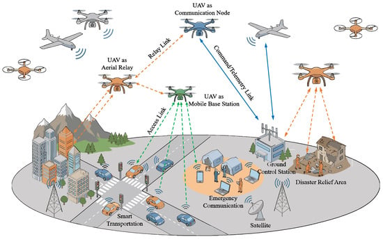
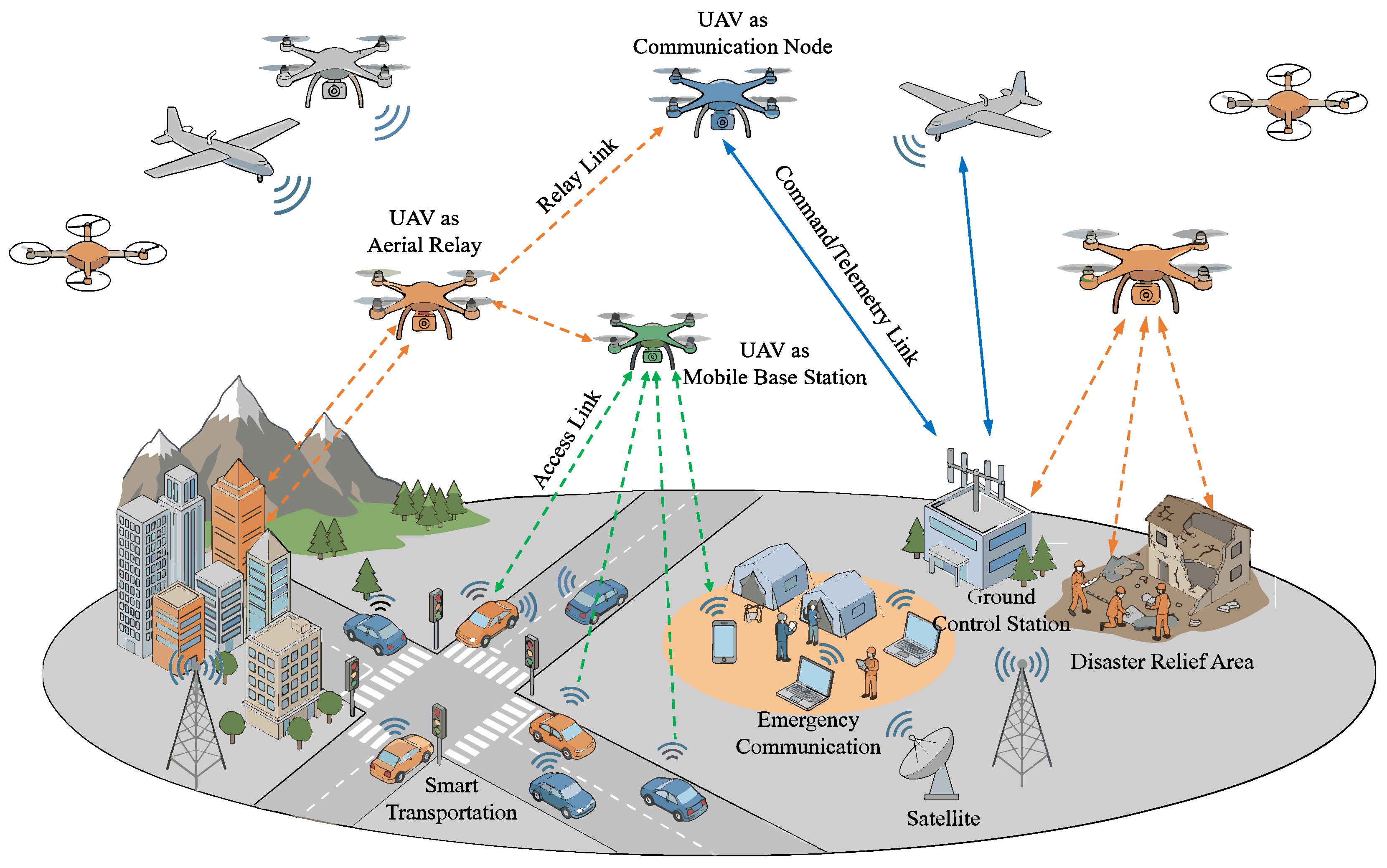
UAVs, due to their high maneuverability, flexibility, and cost-effectiveness, have become an essential component of integrated air–ground networks in the 6G era [1,2]. Leveraging their rapid mobility and line-of-sight enhancement capabilities, UAVs can establish reliable air-to-ground links in complex environments, enabling efficient information exchange and service coverage [3]. As depicted in Figure 1, in UAV communication systems, UAVs not only serve as communication nodes interacting with ground control stations via a data link to support command-and-control functions, including remote control, telemetry, and image transmission [4], but also serve as mobile aerial base stations or relay nodes [5]. Consequently, UAVs have been extensively adopted in a variety of application scenarios, such as disaster response, intelligent transportation, and emergency communications [6,7,8].

Figure 1. UAV communication scenario diagram.

With the expansion of UAV applications, the increasing prevalence of formation flying and high-density deployments and the continual growth in the number of ground terminals, the demand for wireless communication spectrum has risen sharply, exacerbating the conflict between limited spectrum resources and capacity requirements. To alleviate spectrum scarcity and improve spectrum utilization, cognitive radio technology based on dynamic spectrum access mechanisms has been proposed [9,10], enabling secondary users such as UAVs to opportunistically exploit idle frequency bands licensed to primary users [11,12,13], thereby enhancing spectrum efficiency. Within this framework, spectrum sensing serves as a core component, requiring fast and reliable detection of spectrum holes without causing interference to primary users [14], providing a basis for UAV dynamic access and interference avoidance decisions.

In the complex electromagnetic environment of UAV air–ground communications, variations in line-of-sight and non-line-of-sight (LoS/NLoS) conditions can cause fluctuations in channel statistics, while platform mobility introduces Doppler shifts and carrier frequency offsets, leading to a sample-by-sample phase rotation in the received signal and degrading feature stability. Under such air–ground link uncertainties, conventional spectrum sensing methods, such as energy detection (ED) [15,16], matched filter detection (MFD) [17,18], and cyclostationary feature detection (CFD) [19], have been widely studied, but they still exhibit notable limitations in UAV communication scenarios. Specifically, ED is sensitive to noise uncertainty and experiences severe performance degradation in low signal-to-noise ratio (SNR) regimes. MFD requires prior knowledge of the primary user, which is often difficult to obtain and maintain in highly dynamic UAV communications. Although CFD can leverage periodic statistical properties to improve discrimination performance under low SNR, it typically entails high computational complexity and long observation durations, making it challenging to satisfy the low-latency decision requirements of UAV systems.

Recently, deep learning has demonstrated considerable potential for signal detection due to its end-to-end feature learning capability. In particular, convolutional neural networks (CNNs) have been widely adopted for spectrum sensing because of the efficient spatial feature extraction ability [20,21,22,23]. For example, Ni et al. [20] proposed a spectrum sensing approach based on a temporal convolutional network (TCN), exploiting temporal characteristics of the received signal to mitigate the impact of noise uncertainty. Gai et al. [21] employed a dual-branch convolutional architecture to enhance feature extraction. To address the performance degradation of conventional spectrum sensing under generalized noise, Mehrabian et al. [22] designed a CNN-based detector that maintains a certain level of robustness across multiple noise models. However, CNNs tend to focus on spatial patterns in the input and may not sufficiently capture long-range temporal dependencies. To this end, Wang et al. [23] introduced ConvLSTM to extract spatiotemporal features from I/Q signals and achieved improved performance at very low SNR, while Mondal et al. [24] incorporated an LSTM after an Inception module to strengthen temporal dependency modeling. Furthermore, since a unidirectional LSTM cannot simultaneously exploit both past and future occupancy correlations, the works in [25,26] combined BiLSTM with CNN to capture bidirectional temporal correlations, thereby improving sensing accuracy at low-SNR.

Beyond network architecture design, an increasing number of works have adopted input preprocessing to improve training efficiency and robustness [27,28,29,30,31,32,33,34]. Regarding second-order statistical features, the covariance matrix has been used as the input to capture correlation and statistical characteristics [27,28,29]. For instance, Liu et al. [27] applied a CNN to sample covariance matrices to extract statistical features; Xie et al. [28] further integrated LSTM to learn primary-user activity patterns, improving detection probability at low SNR; and Chen et al. [29] proposed a joint modeling framework that combines covariance matrices with LSTM to learn spatial correlations and temporal dependencies simultaneously. Regarding temporal correlation features, Chae et al. [30] used the autocorrelation function curve as input and employed CNN to extract time-correlation features. In terms of time–frequency representations, the wavelet transform (WT), which provides multiresolution time–frequency analysis, has been leveraged for feature extraction in spectrum sensing [31,32]. For example, Zhen et al. [31] combined WT with ResNet to enhance robustness under low SNR, while Zhao et al. [32] further integrated continuous wavelet transform (CWT) with LSTM to exploit temporal features. In addition, STFT has been extensively used to construct two-dimensional time–frequency matrices [33,34]. For instance, Chen et al. [33] proposed STFT-CNN, which feeds the time–frequency matrix into CNN to strengthen detection capability at low SNR, and Gai et al. [34] combined STFT with the improved residual network to enhance feature learning. Building on this line of work, Wang et al. [35] took STFT spectrograms as input and introduced the convolutional block attention module (CBAM) into residual connections to reinforce time–frequency feature extraction, thereby improving detection performance at low SNR. Despite these advances in feature construction and model design, most existing methods still rely primarily on a single representation domain. As a result, the salient characteristics of the received signal may not be fully captured, and detection performance remains constrained, particularly at low-SNR.

To compensate for the information loss incurred by single-domain representations, multidimensional feature fusion and attention enhancement have emerged as important research directions. Zhang et al. [36] constructed a feature matrix by combining energy statistics, power spectra, cyclostationary features, and I/Q components, and employed SenseNet to learn discriminative representations, thereby improving detection capability under low-SNR conditions. To better capture temporal dependencies, Bai et al. [37] formed a matrix comprising energy, power spectra, and cyclostationary features and fed it into the network, where a GRU and an attention mechanism were introduced to emphasize informative time steps and enhance robustness under low-SNR conditions. In terms of attention enhancement, Wang et al. [38] mapped the received signal into a grayscale image and adopted a residual-dense architecture combined with CBAM, which improves sensing accuracy at low-SNR. Regarding multi-domain fusion, Xu et al. [39] jointly exploited the covariance matrix and WT–STFT time–frequency matrix: features were extracted via a lightweight VAE and ResNet branch, respectively, and then adaptively weighted by a fusion module for final decision making, leading to improved detection performance under complex noise conditions. In addition, Xi et al. [40] used a GRU to model temporal dependencies, applied CNN to FFT-transformed input to capture local frequency-domain features, and achieved dynamic time–frequency fusion via cross-attention.

Nevertheless, existing methods still exhibit notable limitations under low-SNR conditions. First, a single representation domain often fails to sufficiently characterize the salient features of the received signal. Second, most multi-domain approaches rely on feature concatenation or late-stage fusion, yet lack an effective mechanism that can jointly model intra-domain dependencies and inter-domain interactions, thereby preventing the complementary advantages of multi-domain features from being consistently exploited.

However, changes in LoS/NLoS conditions and mobility-induced Doppler shifts and carrier frequency offsets in UAV air–ground links can undermine the stability of received features. Existing deep-learning-based spectrum sensing methods often rely on a single representation domain or fuse multiple domains only through feature concatenation, lacking coordinated modeling of intra-domain dependencies and inter-domain interactions. Moreover, under low-SNR conditions, the randomness of noise realizations in training samples can dominate the learning process, reducing detection robustness in UAV spectrum-sensing scenarios. To address these issues, we propose a dual-stream joint learning framework that represents the received signal as both a time-domain I/Q sequence and an STFT spectrogram, extracts complementary features in parallel, and employs intra-branch self-attention to enhance key dependency modeling and inter-branch cross-attention to enable explicit interaction and adaptive fusion. In addition, during training, NCPT constructs ($H_1$/$H_0$) sample pairs that share the same noise realization and introduces a paired constraint to encourage the network to focus on differences caused by signal presence, thereby suppressing noise-induced randomness during training. The main contributions of this work are summarized as follows:

1.

We propose DSHA, a dual-stream spectrum sensing framework that jointly exploits the raw I/Q sequence and an STFT-based time-frequency representation, enabling parallel learning and fusion of complementary features.

2.

We design a cooperative hybrid-attention mechanism, where self-attention is applied within each stream to enhance key dependency modeling and noise suppression, while cross-attention enables explicit interaction and alignment between the time-domain and time-frequency-domain representations, improving feature consistency and detection stability.

3.

We propose a noise-consistent paired training (NCPT) strategy. During training, we construct $H_1$/$H_0$ sample pairs that share the same noise realization and incorporate a paired constraint into the loss function to guide the network to focus on differences caused by signal presence rather than the random patterns of noise, thereby improving detection robustness under low-SNR conditions. During testing deployment, the model still makes single-sample decisions without additional inference overhead.

4.

Finally, we conduct simulation experiments to evaluate DSHA. The results show that DSHA consistently outperforms the reference methods under both the AWGN benchmark setting and more UAV-relevant conditions with Rician fading and normalized frequency offset.

2. System Model

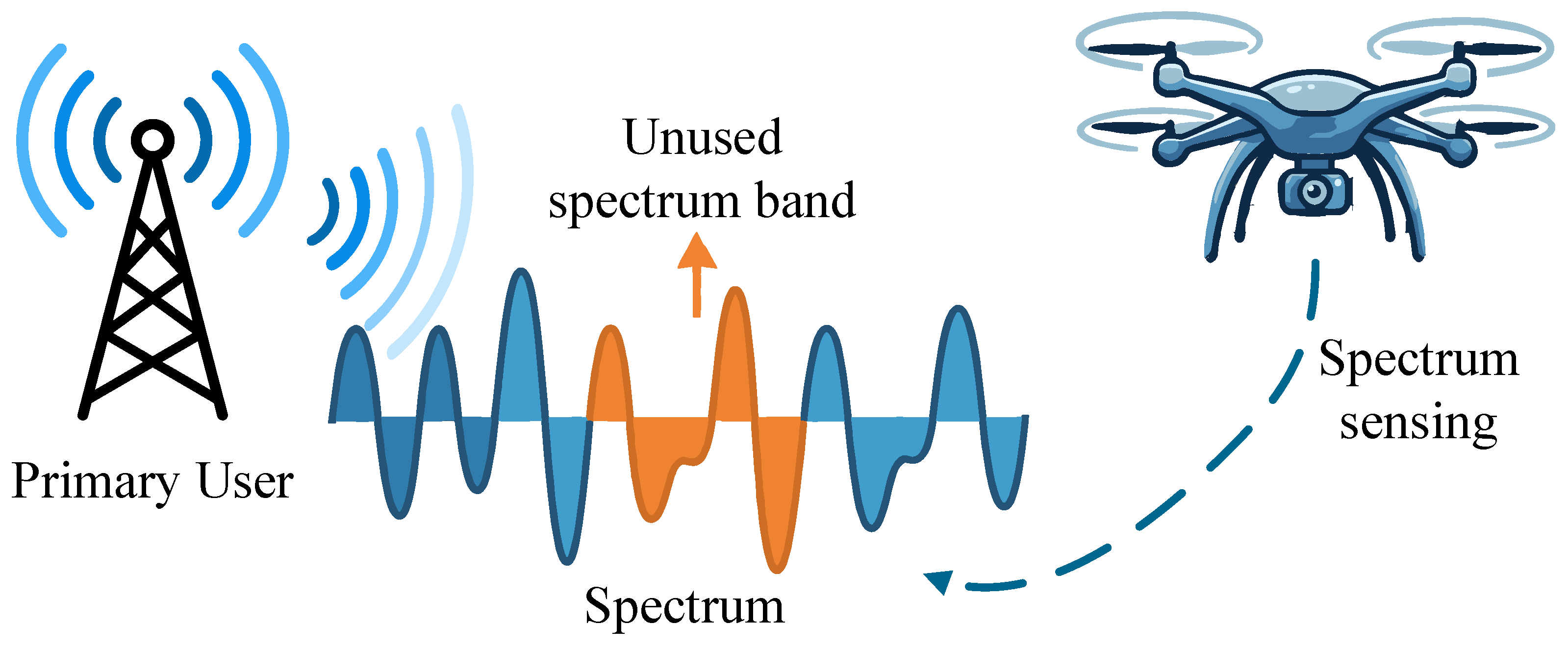
In this work, we consider a cognitive-radio spectrum-sharing scenario for UAV air–ground communications, where the UAV acts as a secondary user (SU) and performs spectrum sensing of an authorized primary user (PU) signal over the target band to determine whether the band is occupied by the PU within the current sensing window. During the ith sensing period, the SU collects a length-N complex baseband discrete received sequence and conducts a binary hypothesis test. To account for propagation variations in UAV air–ground links and mobility-induced synchronization impairments, we model LoS/NLoS condition changes using a Rician fading channel and characterize Doppler shifts and carrier frequency offset using a normalized frequency offset. The system model is illustrated in Figure 2. Spectrum sensing can be formulated as the following binary hypothesis test:

$$\begin{array}{cc}\hfill H_0: & y_i\left[n\right]=u_i\left[n\right],\hfill \end{array}$$

(1)

$$\begin{array}{cc}\hfill H_1: & y_i\left[n\right]=h_i{s}_i\left[n\right]e^{j2\pi {\epsilon }_{i}n}+u_i\left[n\right],\hfill \end{array}$$

(2)

where $s_i\left[n\right]$ denotes the nth complex baseband sample of the PU transmitted signal, $u_i\left[n\right]$∼$\mathcal{CN}(0, {\sigma }^2)$ is additive white Gaussian noise (whose I/Q components can be regarded as independent zero-mean real Gaussian random variables), $h_i$ is the complex fading coefficient of the air–ground link, and ${\epsilon }_i$ is the normalized frequency offset, used to represent the combined effect of Doppler shift and carrier frequency offset. It can be expressed as

$$\begin{array}{c}{\epsilon }_i={\displaystyle \frac{△f_i}{F_s}}\end{array}$$

(3)

$$\begin{array}{c}△f_i=f_{D,i}+f_{CFO,i},\end{array}$$

(4)

where $F_s$ is the sampling rate and $△f_i$ is the total frequency offset, composed of the Doppler shift $f_{D,i}$ and the carrier frequency offset $f_{CFO,i}$. Since the sensing window is short, we treat ${\epsilon }_i$ as approximately constant within each window.

$$h_i=\sqrt{{\displaystyle \frac{K}{K+1}}}{h}_{i,LoS}+\sqrt{{\displaystyle \frac{1}{K+1}}}{h}_{i,NLoS},$$

(5)

where K is the Rician factor, which measures the relative strength of the LoS component with respect to the scattered component, $h_{i,NLoS}$∼$\mathcal{CN}(0,1)$ and $h_{i,LoS}=e^{j{\varphi }_k}$ (where ${\varphi }_k$ is the phase).

Figure 2. System model.

For convenience, we let ${\mathbf{y}}_{\mathbf{i}}=y_i\left[0\right],y_i\left[1\right],\dots ,y_i{[N-1]]}^{\mathrm{T}}$, ${\mathbf{s}}_{\mathbf{i}}={[s_i\left[0\right],s_i\left[1\right],\dots ,s_i[N-1]]}^{\mathrm{T}}$, and ${\mathbf{u}}_{\mathbf{i}}={[u_i\left[0\right],u_i\left[1\right],\dots ,u_i[N-1]]}^{\mathrm{T}}$. Then, under $H_1$, the received vector can be written as

$${\mathbf{y}}_{\mathbf{i}}=h_{i}D\left({\epsilon }_i\right){\mathbf{s}}_{\mathbf{i}}+{\mathbf{u}}_{\mathbf{i}},$$

(6)

where $D\left({\epsilon }_i\right)=diag(1,e^{j2\pi {\epsilon }_i},\dots ,e^{j2\pi {\epsilon }_i(N-1)})$. When $h_i=1$ and ${\epsilon }_i=0$, the above model reduces to the AWGN benchmark setting, which is used to ensure comparability with the comparison methods.

Spectrum sensing performance is commonly evaluated in terms of the detection probability $P_d$ and the false-alarm probability $P_f$, which are defined as

$$\begin{array}{cc}\hfill P_d& =P\{H_1\mid H_1\},\hfill \end{array}$$

(7)

$$\begin{array}{cc}\hfill P_f& =P\{H_1\mid H_0\},\hfill \end{array}$$

(8)

where $P_d$ denotes the probability of correctly detecting the PU signal when it is present and $P_f$ denotes the probability of falsely declaring the presence of the PU signal when only noise is present.

3. DSHA Spectrum Sensing Algorithm

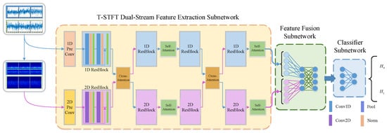
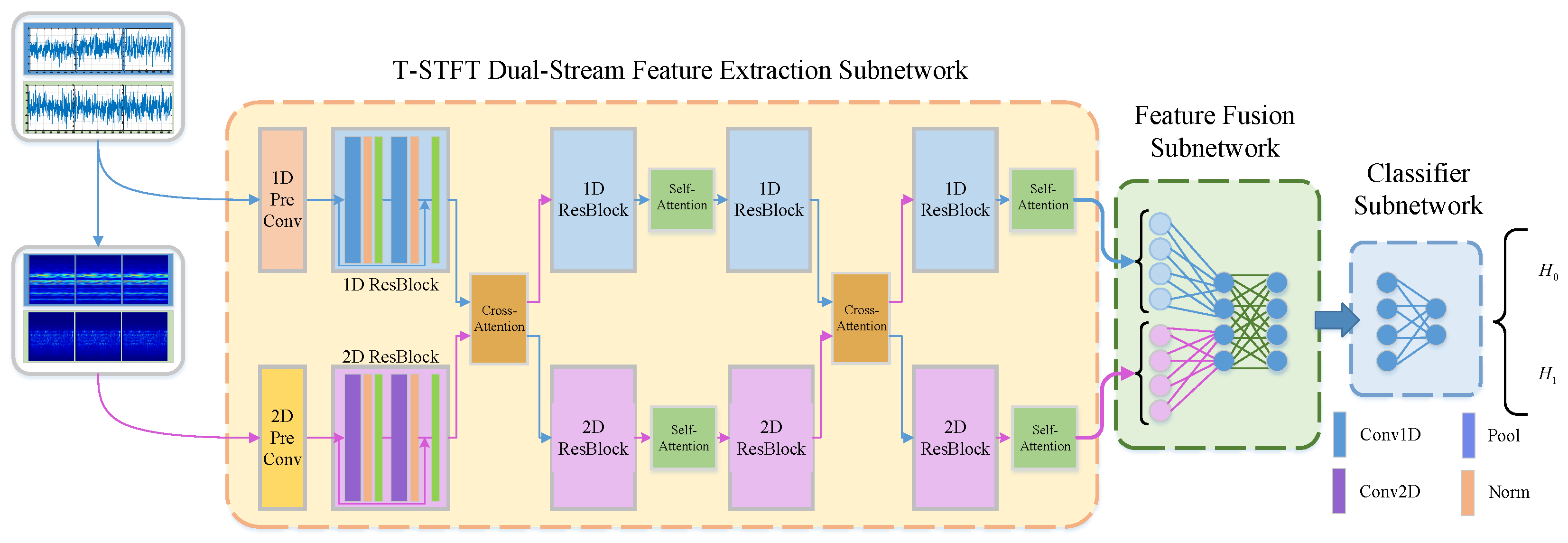
In UAV air–ground spectrum sharing scenarios, the received signal is affected not only by noise but also by variations in LoS/NLoS conditions and mobility-induced Doppler shifts and carrier frequency offsets, causing the observed features to fluctuate with channel conditions and thus reducing feature stability. As a result, a single representation domain often cannot provide sufficiently stable and informative features. Moreover, multi-domain approaches that rely only on late-stage concatenation or simple fusion may fail to fully exploit complementary information across domains. To address these issues, we propose a dual-stream hybrid-attention spectrum sensing network, termed DSHA. It constructs two complementary representations from the received signal, a time-domain I/Q sequence and an STFT spectrogram, and incorporates self-attention within each branch to strengthen intra-domain dependency modeling. It also uses cross-attention between branches to enable explicit interaction and adaptive fusion, thereby improving detection stability under Rician fading and frequency-offset perturbations. The overall framework of DSHA is illustrated in Figure 3.

Figure 3. DSHA spectrum sensing framework.

The received signal $y\left(n\right)$ is represented as a time-domain sequence and the corresponding time-frequency representation after preprocessing, which are fed into the network as dual-stream inputs to exploit complementary information across domains and provide multidimensional representations for subsequent processing. As shown in Figure 3, the DSHA model consists of three subnetworks, namely the T-STFT dual-stream feature extraction subnetwork, the feature fusion subnetwork, and the classification subnetwork. The time-domain branch and the time-frequency branch extract intra-domain features from their respective inputs. To better capture time-frequency characteristics and improve cross-domain feature interaction, we introduce a hybrid attention mechanism in the dual-stream feature extraction subnetwork, enabling intra-domain information modeling and cross-domain feature complementarity. The high-level features from the two streams are then fed into the feature fusion subnetwork to obtain a joint representation. Finally, the classification subnetwork, composed of fully connected layers, outputs the decision result. The network configuration of DSHA is summarized in Table 1.

Table 1. DSHA network parameters.

Block	OutputSize	OriSubNet	STFT SubNet	BlockNum
ConvBlock1	$16\times 1024/16\times 128\times 128$	$\left[\begin{array}{c}\mathrm{Conv}1\mathrm{D}\left(\mathrm{k}3\mathrm{s}1\right)\\ \mathrm{BN}+\mathrm{LReLU}\end{array}\right]$	$\left[\begin{array}{c}\mathrm{Conv}2\mathrm{D}\left(\mathrm{k}3\mathrm{s}1\right)\\ \mathrm{BN}+\mathrm{LReLU}\end{array}\right]$	×2
ResBlock1	$16\times 1024/16\times 128\times 128$	$\left[\begin{array}{c}\mathrm{Conv}1\mathrm{D}\left(\mathrm{k}3\mathrm{s}1\right)\\ \mathrm{BN}+\mathrm{LReLU}\\ \mathrm{Conv}1\mathrm{D}\left(\mathrm{k}3\mathrm{s}1\right)\\ \mathrm{BN}+\mathrm{Add}+\mathrm{LReLU}\end{array}\right]$	$\left[\begin{array}{c}\mathrm{Conv}2\mathrm{D}\left(\mathrm{k}3\mathrm{s}1\right)\\ \mathrm{BN}+\mathrm{LReLU}\\ \mathrm{Conv}2\mathrm{D}\left(\mathrm{k}3\mathrm{s}1\right)\\ \mathrm{BN}+\mathrm{Add}+\mathrm{LReLU}\end{array}\right]$	×2
Down1	$32\times 512/32\times 64\times 64$	$\left[\begin{array}{c}\mathrm{Conv}1\mathrm{D}\left(\mathrm{k}3\mathrm{s}2\right)\\ \mathrm{BN}+\mathrm{LReLU}\end{array}\right]$	$\left[\begin{array}{c}\mathrm{Conv}2\mathrm{D}\left(\mathrm{k}3\mathrm{s}2\right)\\ \mathrm{BN}+\mathrm{LReLU}\end{array}\right]$
MixBlock	$32\times 512/32\times 64\times 64$	$\left[\begin{array}{cc}\mathrm{Conv}1\mathrm{D}\left(\mathrm{k}1\mathrm{s}1\right)& \mathrm{Conv}2\mathrm{D}\left(\mathrm{k}1\mathrm{s}1\right)\\ \mathrm{Conv}1\mathrm{D}\left(\mathrm{k}1\mathrm{s}1\right)& \mathrm{Conv}2\mathrm{D}\left(\mathrm{k}1\mathrm{s}1\right)\\ \mathrm{Pool}1\mathrm{D}+\mathrm{Linear}& \mathrm{Pool}2\mathrm{D}+\mathrm{Linear}\\ \mathrm{Softmax}& \mathrm{Softmax}\\ \mathrm{Multiplication}& \mathrm{Multiplication}\end{array}\right]$	–
ResBlock2	$32\times 512/32\times 64\times 64$	$\left[\begin{array}{c}\mathrm{Conv}1\mathrm{D}\left(\mathrm{k}3\mathrm{s}1\right)\\ \mathrm{BN}+\mathrm{LReLU}\\ \mathrm{Conv}1\mathrm{D}\left(\mathrm{k}3\mathrm{s}1\right)\\ \mathrm{BN}+\mathrm{Add}+\mathrm{LReLU}\end{array}\right]$	$\left[\begin{array}{c}\mathrm{Conv}2\mathrm{D}\left(\mathrm{k}3\mathrm{s}1\right)\\ \mathrm{BN}+\mathrm{LReLU}\\ \mathrm{Conv}2\mathrm{D}\left(\mathrm{k}3\mathrm{s}1\right)\\ \mathrm{BN}+\mathrm{Add}+\mathrm{LReLU}\end{array}\right]$
Down2	$64\times 256/64\times 32\times 32$	$\left[\begin{array}{c}\mathrm{Conv}1\mathrm{D}\left(\mathrm{k}3\mathrm{s}2\right)\\ \mathrm{BN}+\mathrm{LReLU}\end{array}\right]$	$\left[\begin{array}{c}\mathrm{Conv}2\mathrm{D}\left(\mathrm{k}3\mathrm{s}2\right)\\ \mathrm{BN}+\mathrm{LReLU}\end{array}\right]$
AttentionBlock	$64\times 256/64\times 32\times 32$	$\mathrm{Attention}1\mathrm{D}$	$\mathrm{Attention}2\mathrm{D}$
LinearBlock1	1024	$\mathrm{Linear}$	$\mathrm{Linear}$	×1
LinearBlock2	2	$\left[\begin{array}{c}\mathrm{BN}+\mathrm{LReLU}\\ \mathrm{Linear}\\ \mathrm{BN}+\mathrm{LReLU}\\ \mathrm{Linear}\end{array}\right]$

3.1. Dual Stream Input Representation

To exploit the complementary information of the received signal across different representation domains, we construct dual-stream inputs. The time-domain stream directly processes the I/Q sequence, whereas the time-frequency stream applies a time-frequency transform to the same sequence to obtain a time-frequency map. The input to the time-domain stream is defined as

$$\begin{array}{cc}\hfill {\mathit{X}}_{\mathrm{time}}& =\left[\begin{array}{cc}\Re \left\{y\right[0\left]\right\}& \Im \left\{y\right[0\left]\right\}\\ \Re \left\{y\right[1\left]\right\}& \Im \left\{y\right[1\left]\right\}\\ ⋮& ⋮\\ \Re \left\{y\right[N-1\left]\right\}& \Im \left\{y\right[N-1\left]\right\}\end{array}\right]\in {\mathbb{R}}^{N\times 2}\hfill \end{array}$$

(9)

where $\Re \{·\}$ and $\Im \{·\}$ denote the real-part and imaginary-part operators, respectively.

To facilitate hierarchical downsampling and align with the network architecture, the received sequence is length-aligned before being fed into DSHA. Specifically, the original sequence of length $N=1000$ is extended to $N_p=1024$ via zero padding. The subsequent time-domain I/Q representation and the STFT transformation are both constructed based on the aligned sequence.

Since the short-time Fourier transform (STFT) converts a one-dimensional signal into a two-dimensional time-frequency representation that is amenable to convolutional neural networks, we adopt STFT as the time-frequency mapping in the time-frequency stream. STFT performs the transformation from a one-dimensional signal to a two-dimensional time-frequency map via a sliding window function. We let $g[\ell ]$ denote the window function with window length $L_w$, frame shift R, and number of frequency bins $K_{fc}$. Then, the STFT can be expressed as

$$Y[m,k]=\sum _{\ell =0}^{L_w-1}y[\ell +mR]g[\ell ]e^{-j{\displaystyle \frac{2\pi k}{K_{fc}}}\ell },$$

(10)

where, $m\in \{0,1,\dots ,M-1\}$ and $k\in \{0,1,\dots ,K_{fc}-1\}$ denote the frame index and the frequency index, respectively. $K_{fc}$ is the number of frequency bins, and M is the number of frames, which is determined by N, L and R. Accordingly, the STFT output is collected into a time-frequency matrix $\mathbf{Y}\in {\mathbb{C}}^{M\times K_{fc}}$. We take its magnitude and apply linear normalization to obtain the input to the time-frequency branch, which can be expressed as

$${\mathit{X}}_{\mathit{tf}}={\displaystyle \frac{\left|\mathit{Y}\right|-\min \left(\right|\mathit{Y}\left|\right)}{\max \left(\right|\mathit{Y}\left|\right)-\min \left(\right|\mathit{Y}\left|\right)}},$$

(11)

where $\left|·\right|$ denotes the magnitude operator and $\max \left(\right|\mathit{Y}\left|\right)$ and $\min \left(\right|\mathit{Y}\left|\right)$ represent the maximum and minimum values in the sample, respectively. This normalization helps eliminate scale variations and facilitates network training. In this work, we adopt the Hamming window as the window function to suppress spectral leakage. It is worth noting that the time-domain I/Q representation preserves phase information and can capture instantaneous variations. In contrast, the time-frequency branch uses the STFT magnitude spectrogram as input, which can to some extent reduce the impact of phase rotation caused by normalized frequency offset $\epsilon$ on the learned representation. These two representations are complementary, which helps to improve detection stability under frequency-offset perturbations.

3.2. T-STFT Dual-Stream Feature Extraction Subnetwork

To fully exploit the complementarity of the received signal in time-domain and time-frequency representations, we design a T-STFT dual-stream feature extraction structure. The network contains two branches, with one processing the received time-domain signal and the other processing the time-frequency map obtained via STFT. In the low-SNR regime, a single time-domain or time-frequency-domain representation often fails to provide sufficient discriminative features. Therefore, features are extracted from low-SNR signals in two different representation spaces, and cross-branch interaction is employed to enable complementary feature integration. This alleviates the insufficient informative cues in a single feature space and thereby improves spectrum sensing accuracy.

As shown in Figure 3 and Table 1, in the time-domain stream, we build a time-domain feature extraction branch based on one-dimensional convolutional layers, since the PU signal is one-dimensional. This branch performs modeling and feature extraction on ${\mathit{X}}_{\mathrm{time}}$. Compared with commonly used fully connected networks, one-dimensional convolutions involve fewer parameters, run faster, and are easier to train. The backbone of the branch is constructed by stacking a series of residual blocks, which facilitates training even with increased network depth. Each residual block consists of two 1D convolutional layers, and each convolution is followed by a batch normalization (BN) layer and a LeakyReLU activation. After each residual block, a stride-2 convolutional layer is applied for feature downsampling to progressively enlarge the receptive field and extract multi-scale features. Notably, Transformer-based self-attention modules are appended after the second and fourth residual blocks to help the network extract informative signal-related features in the presence of strong noise. Cross-attention modules are appended after the first and third residual blocks. These modules leverage features transferred from the time-frequency branch to guide feature extraction in the time branch, thereby enhancing the feature extraction capability of the network in the low-SNR regime. The hybrid attention mechanism is described in detail in the next subsection.

In the time-frequency stream, the input is the normalized time-frequency magnitude matrix obtained from Equation (10), which exhibits a two-dimensional structure on the time-frequency plane. Accordingly, we construct a time-frequency feature extraction branch based on 2D convolutions to model and extract features from ${\mathit{X}}_{\mathrm{tf}}$. The time-domain branch network and the time-frequency branch network share the same backbone architecture, except that all 1D convolutional layers are replaced with 2D convolutional layers.

We let the two branch networks be denoted as ${\epsilon }_t(·)$ and ${\epsilon }_{t}f(·)$. The resulting feature outputs are

$${\mathit{F}}_t={\epsilon }_t\left({\mathit{X}}_{\mathrm{time}}\right),{\mathit{F}}_{tf}={\epsilon }_t\left({\mathit{X}}_{\mathrm{tf}}\right),$$

(12)

where ${\mathit{F}}_t$ and ${\mathit{F}}_{tf}$ denote the high-level feature representations in the time domain and the time-frequency domain, respectively.

3.3. Cooperative Hybrid Attention Mechanism

In this work, we design a cooperative hybrid attention mechanism to assist the T-STFT dual-stream feature extraction subnetwork in feature learning. The proposed mechanism consists of self-attention for intra-domain dependency enhancement and cross-attention for cross-domain interaction.

3.3.1. Self Attention

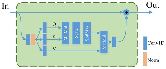
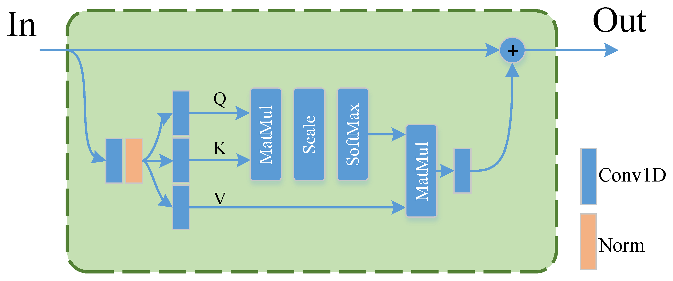
In the low-SNR regime, excessive noise introduced during transmission may cause the PU signal in the received samples to be submerged in noise. Noise becomes dominant in the observations, which may lead the network to learn feature representations dominated by noise and thus reduce the separability between $H_1$ and $H_0$. To strengthen intra-domain dependency modeling and improve the stability of feature representations, we insert Transformer-inspired self-attention modules into both branches, as illustrated in Figure 4. The self-attention module adaptively reweights features using global context, which helps emphasize more consistent dependencies and suppress spurious responses induced by noise, thereby improving the stability of intra-domain feature representations. The module is plug-and-play, with the same input and output dimensions and number of channels, so it can be inserted without modifying the existing network structure or feature dimensionality.

Figure 4. Self-attention module.

As shown in Figure 4, the self-attention module contains an input feature map and an output feature map, and the input and output have exactly the same shape. The module consists of two parts. One part directly retains the input feature $\mathit{X}$. The other part first passes $\mathit{X}$ through a convolutional layer and a LayerNorm layer in sequence to obtain the preprocessed input feature $\tilde{\mathit{X}}$, whose size remains unchanged. Then, $\tilde{\mathit{X}}$ is fed into three parallel convolutional layers to generate the Query, Key, and Value (denoted as $\mathit{Q}$, $\mathit{K}$, and $\mathit{V}$), respectively:

$$\mathit{Q}=\tilde{\mathit{X}}{W}_Q,\mathit{K}=\tilde{\mathit{X}}{W}_K,\mathit{V}=\tilde{\mathit{X}}{W}_V,$$

(13)

where ${\mathit{W}}_Q$, ${\mathit{W}}_K$ and ${\mathit{W}}_V$ are learnable projection matrices. The Query represents the features that the module needs to attend to, the Key represents the identifiers of all features in the current input, and the Value represents the actual information of all features in the current input. Each Key identifier corresponds one-to-one to the associated Value. Then, the scaled dot-product attention is computed as follows:

$$\mathit{A}=\mathrm{Softmax}\left({\displaystyle \frac{\mathit{Q}{\mathit{K}}^T}{\sqrt{d}}}\right),\mathit{Z}=\mathit{A}\mathit{V},$$

(14)

where $\mathrm{Softmax}(·)$ normalizes the attention weights for each query, d is the feature dimension, $\mathit{A}$ denotes the attention weight matrix, and $\mathit{Z}$ denotes the aggregated feature from the second part. Finally, the module output is obtained by summation as follows:

$$\mathrm{S}\mathrm{A}\left(\mathit{X}\right)=\mathit{X}+\mathit{Z}.$$

(15)

As shown in Equations (14) and (15), we compute the scaled dot product between the Query and Key and apply Softmax to obtain the attention weight matrix, which is then used to compute a weighted sum of the Value to produce the aggregated features. Larger weights in $\mathit{A}$ indicate that the corresponding features require more attention, thereby emphasizing key dependencies and suppressing noise-dominated responses. The normalized attention weights are then multiplied with the Value to extract the features that should be attended to. Finally, the extracted features are added to the module input to obtain the output feature.

It should be noted that, in the time-domain branch, the projection layers within the self-attention module are implemented with 1D convolutions to match sequential features, whereas in the time-frequency branch, 2D convolutions are used to match two-dimensional time-frequency features. Since this module preserves the input and output dimensions, it can be flexibly inserted into different residual stages to enhance intra-domain dependency modeling.

3.3.2. Cross Attention

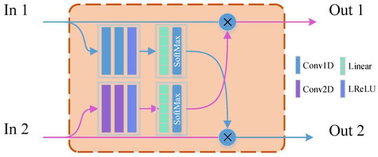
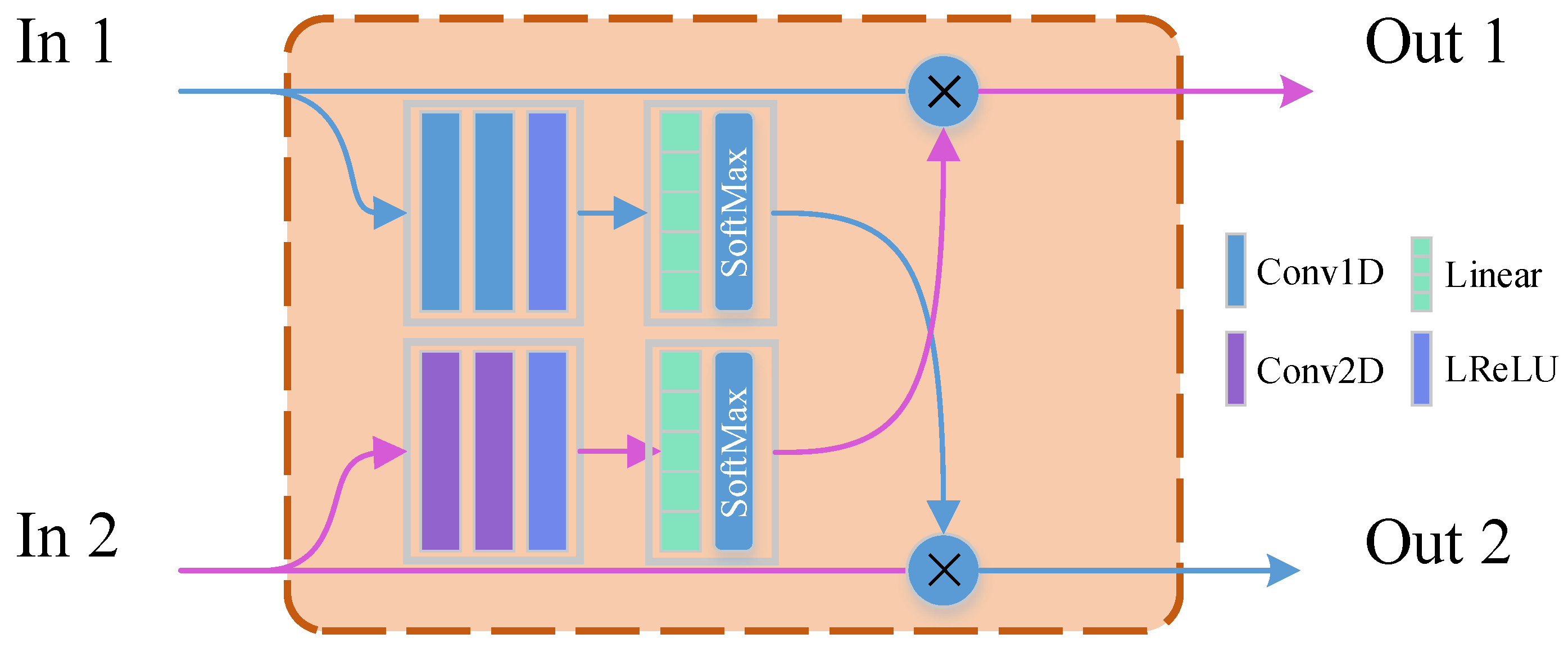
In low-SNR regime, the PU signal and noise are severely entangled, making it difficult to separate signal-related and noise-related features within a single representation domain (time domain only or time-frequency domain only). To better exploit the complementarity between time-domain and time-frequency representations, we design a cross-attention module to enable explicit interaction between the two domains, as illustrated in Figure 5. Unlike the self-attention module, which operates on a single branch, the cross-attention module acts on both branches simultaneously. Specifically, features from the time-domain branch are used to generate channel-wise guidance for the time-frequency branch, while features from the time-frequency branch are used to generate channel-wise guidance for the time-domain branch, thereby achieving bidirectional interaction and cooperative modeling of complementary features.

Figure 5. Cross-attention module.

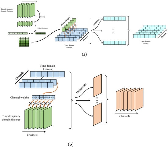
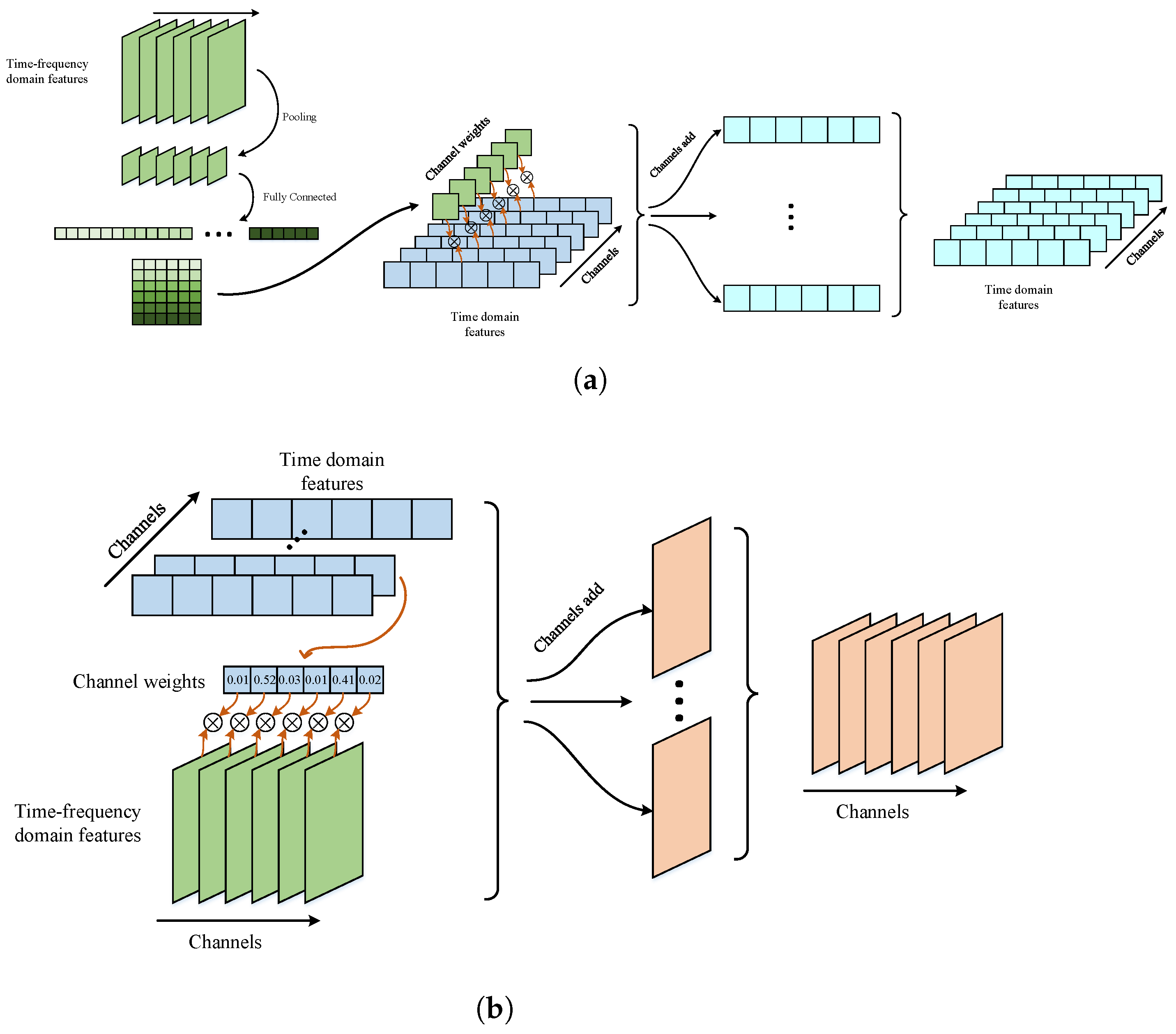
The implementation details of the cross-attention module are illustrated in Figure 6, and its insertion locations and network settings are summarized in Table 1. As listed in Table 1, this module is inserted after the first and third residual blocks in both branches. Since it preserves the input and output scales, it can be integrated with the residual backbone without changing the feature dimensionality. The cross-attention module takes feature inputs from both the time-domain and time-frequency branches and outputs the processed features for the two branches. For each branch, the input and output features have the same size. Taking the time-domain → time-frequency-domain direction as an example, the input features of Branch 1 (time-domain branch) are successively passed through two 1D convolutional layers and one pooling layer for feature compression and aggregation, where a LeakyReLU activation follows the first convolutional layer. The resulting features are then fed into a fully connected layer to generate a channel-weight vector for guiding Branch 2. The output contains $C_{tf}^2$ elements and is reshaped into a $C_{tf}\times C_{tf}$ channel-weight matrix. A row-wise Softmax normalization is applied to obtain a channel-mixing matrix, which is used to form a weighted combination of the channels in Branch 2 (time-frequency branch). The reverse direction time-frequency → time domain is implemented in the same manner, except that 2D convolutions are used in the weight-generation path to match time-frequency features.

Figure 6. Cross-attention module detailed schematic diagram. (a) STFT-Temporal Attention Mechanism. (b) Temporal-STFT Attention Mechanism.

The above procedure is equivalent to constructing a channel-mixing matrix normalized by a row-wise Softmax and using this matrix to form a weighted linear combination of the channels in the target branch. For a formal description, we take the time-domain → time-frequency direction as an example. We let the input feature of the time-frequency branch be ${\mathbf{F}}_{tf}^{in}\in {\mathbb{R}}^{C_{tf}\times H_f\times W_f})$, where $C_{tf}$ denotes the number of channels and $H_f$, $W_f$ denotes the spatial size. A channel-mixing matrix is generated from the time-domain feature ${\mathbf{F}}_t$ via a mapping ${\varphi }_{t\to tf}(·)$ and is normalized by a row-wise Softmax as follows:

$${\mathbf{A}}_{t\to tf}={\mathrm{Softmax}}_{row}\left({\varphi }_{t\to tf}\left({\mathbf{F}}_t\right)\right)\in {\mathbb{R}}^{C_{tf}\times C_{tf}},$$

(16)

where ${\varphi }_{t\to tf}(·)$ denotes the composite mapping of convolution, pooling, and fully connected layers, which outputs $C_{tf}^2$ elements and reshapes them into a matrix; ${\mathrm{Softmax}}_{row}$ denotes row-wise Softmax normalization, such that the weights in each row sum to 1. The resulting channel-mixing matrix is then used to linearly combine the channels of the time-frequency branch, yielding the updated time-frequency feature:

$${\mathbf{F}}_{tf}^{out}\left(c\right)=\sum _{c^{\prime }=1}^{C_{tf}}{\mathbf{A}}_{t\to tf}(c,c^{\prime }){\mathbf{F}}_{tf}^{in}\left(c^{\prime }\right),c=1,\dots ,C_{tf},$$

(17)

where ${\mathbf{F}}_{tf}^{in}\left(c^{\prime }\right)$ denotes the input feature map of the $c^{\prime }$th channel and ${\mathbf{F}}_{tf}^{out}\left(c\right)$ denotes the output feature map of the cth channel. The time-frequency → time-domain direction is defined in the same manner, where ${\mathbf{A}}_{tf\to t}$ is generated from the time-frequency branch and is used to update the time-domain features via channel mixing. Together, the two directions constitute a bidirectional interaction mechanism, which injects time-frequency information into the time-domain space and time-domain information into the time-frequency space. This enables cooperative modeling of complementary cross-domain features, thereby improving discriminability and detection robustness in the low-SNR regime.

3.4. Feature Fusion and Classification

After T-STFT dual-stream feature extraction and cooperative hybrid-attention enhancement, two high-level feature representations, ${\mathbf{F}}_t$ and ${\mathbf{F}}_{tf}$, are obtained. For notational simplicity, we continue to use ${\mathbf{F}}_t$ and ${\mathbf{F}}_{tf}$ to denote the two attention-enhanced feature outputs in the following. Since the two feature streams have different dimensional forms, they are first compressed into one-dimensional vector representations, ${\overline{\mathbf{F}}}_t$ and ${\overline{\mathbf{F}}}_{tf}$, and then fed into fully connected layers for fusion and classification.

Specifically, dimensionality reduction mappings are applied to the two feature streams, and the resulting vectors are concatenated. The fused feature ${\mathbf{F}}_t$ is then obtained via a fusion mapping as follows:

$$\mathbf{h}={\Psi }_f\left([{\Psi }_t\left({\overline{\mathbf{F}}}_t\right);{\Psi }_{tf}\left({\overline{\mathbf{F}}}_{tf}\right)]\right),$$

(18)

where ${\Psi }_t(·)$ and ${\Psi }_{tf}(·)$ denote the dimensionalitycreduction mappings for the two streams, ${\Psi }_f(·)$ denotes the fusion mapping, and $[·;·]$ denotes the concatenation operation.

In the classification stage, an MLP is adopted to perform binary decision on the fused feature h, and output the probability of signal presence:

$$z=w^{\mathrm{T}}\mathbf{h}+b,p=\sigma \left(z\right),$$

(19)

where w and b are the classifier parameters, $p\in (0,1)$ is the output probability, $\sigma (·)$ denotes the Sigmoid activation function and $\sigma \left(z\right)={\displaystyle \frac{1}{1+e^{-z}}}$. The parameter configuration of the fusion and classification module is given by LinearBlock in Table 1.

4. Noise-Consistent Paired Training

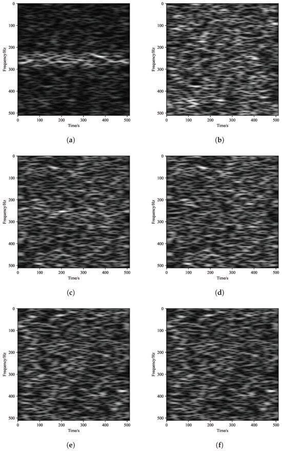
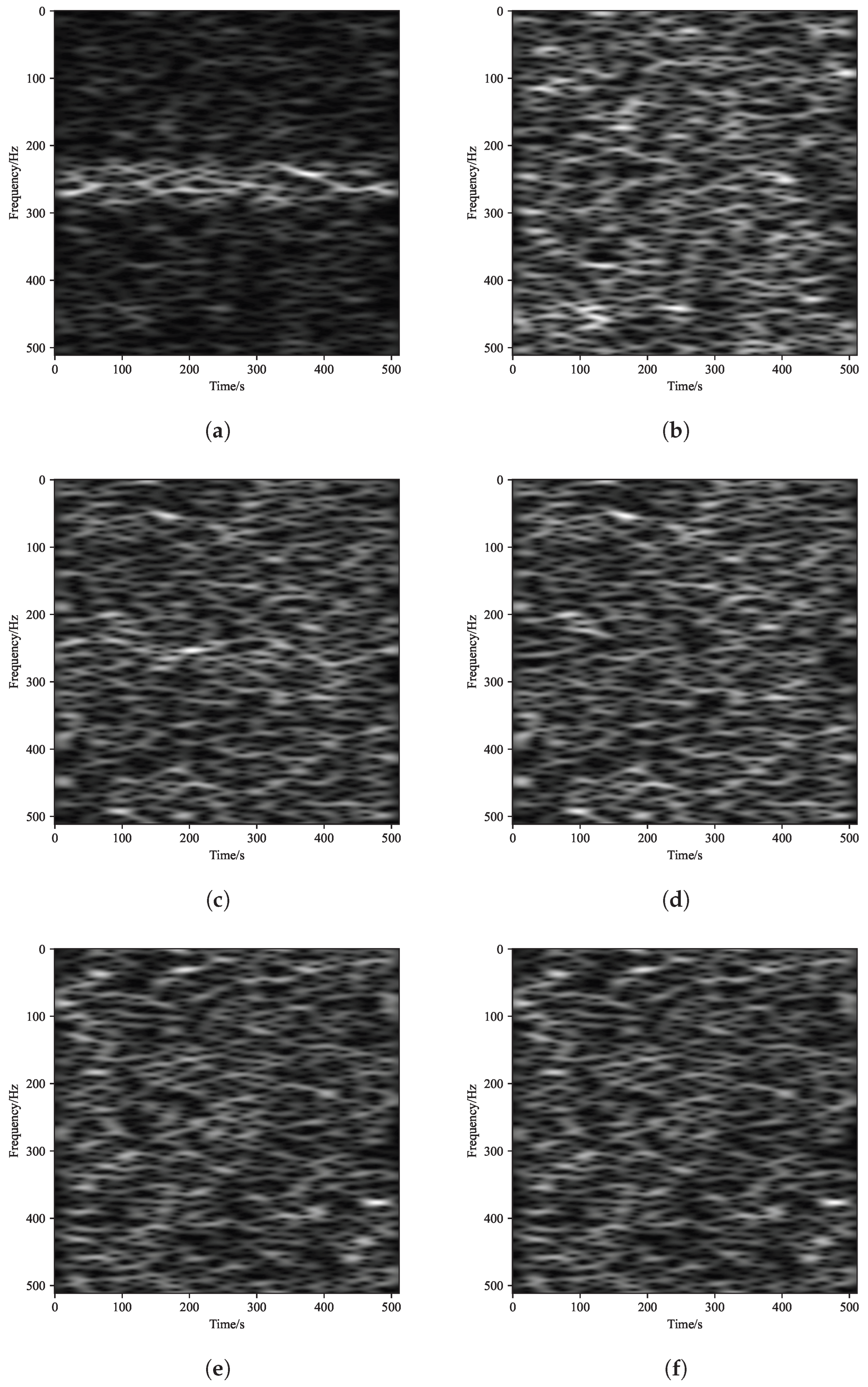
In the low-SNR regime, the discriminative features of the PU signal are often submerged in noise, resulting in a markedly reduced observation gap between $H_1$ and $H_0$. To provide an intuitive view of the signal energy distribution in the time-frequency domain and the separability between $H_1$ and $H_0$ as the SNR varies, we apply STFT to the received sequence. Figure 7 presents the STFT magnitude spectrograms for $H_1$ and $H_0$ at SNRs of 0 dB, −10 dB and −20 dB. The spectrograms are generated via Python 3.7 simulations and visualized in grayscale, where the horizontal axis denotes time, the vertical axis denotes frequency, and the pixel intensity represents the normalized magnitude at each time-frequency bin.

Figure 7. Comparison of the time-frequency representations of the received signal $y\left[n\right]$ under $H_1$ and $H_0$ at different SNRs. (a) Time-frequency representation under $H_1$ at SNR = 0 dB; (b) Time-frequency representation under $H_0$ at SNR = 0 dB; (c) Time-frequency representation under $H_1$ at SNR = −10 dB; (d) Time-frequency representation under $H_0$ at SNR = −10 dB; (e) Time-frequency representation under $H_1$ at SNR = −20 dB; (f) Time-frequency representation under $H_0$ at SNR = −20 dB.

As shown in Figure 7, at the SNR of 0 dB, the time-frequency map under $H_1$ exhibits prominent bright stripes, indicating that the primary-user signal is clearly visible. As the SNR decreases substantially, the signal energy becomes overwhelmed by noise and the time-frequency maps below $H_1$ and $H_0$ become increasingly similar, making the received observations nearly indistinguishable. This is because all noise realizations are independently generated, yielding no explicit correlation between positive and negative samples, and samples are randomly drawn from the dataset. Under moderate-SNR conditions (Figure 7a,b), conventional training performs well because the PU signal dominates the positive samples, making the two classes readily separable. However, its performance degrades markedly in the low-SNR regime, as the PU signal is largely buried in noise, the network struggles to focus on salient PU-discriminative features during learning.

To address this limitation, we propose a noise-consistent paired training (NCPT) strategy, where samples are fed into the network during training in the form of positive–negative pairs that share the same noise realization. For the ith pair, the constructed positive and negative samples can be formulated as

$$\begin{array}{cc}\hfill y_i^{+}\left(n\right)& =h_i{s}_i\left(n\right)e^{j2\pi {\epsilon }_{i}n}+u_i\left(n\right),\hfill \end{array}$$

(20)

$$\begin{array}{cc}\hfill y_i^{-}\left(n\right)& =u_i\left(n\right),\hfill \end{array}$$

(21)

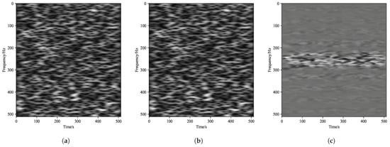
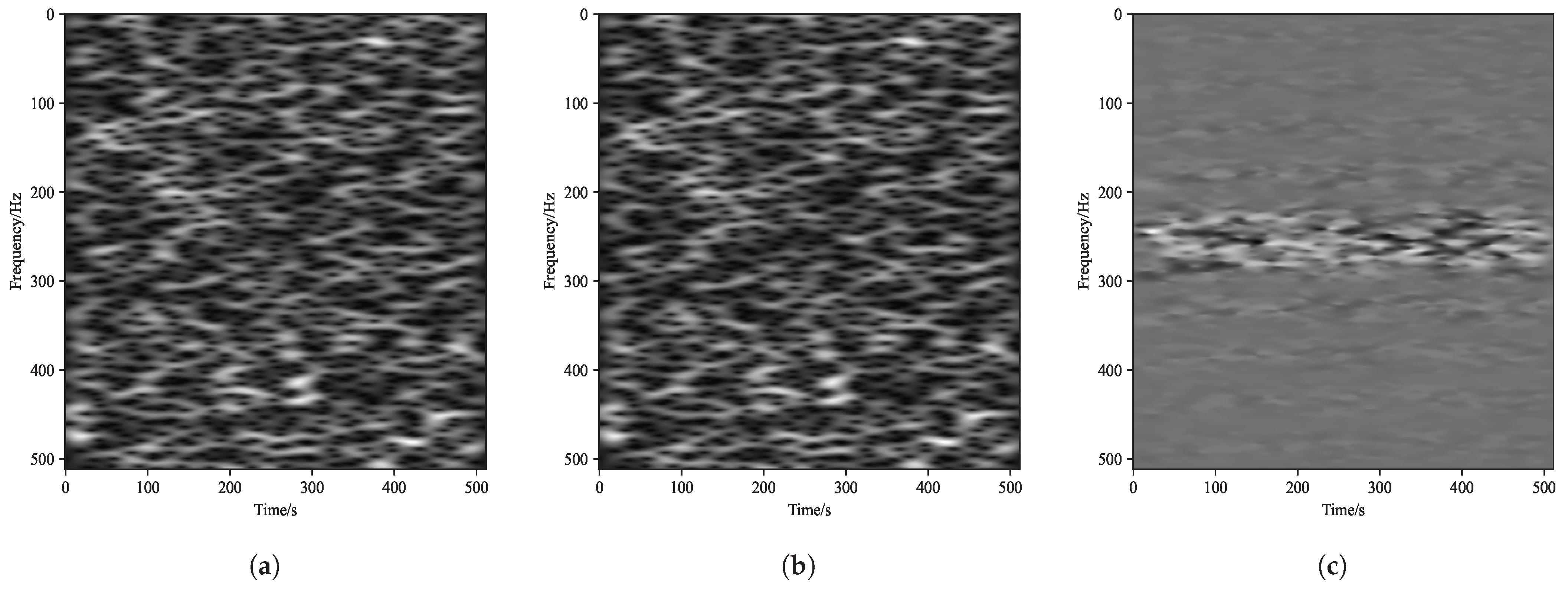
where $y_i^{+}\left(n\right)$ denotes the noise-corrupted signal in the ith sample pair, $y_i^{-}\left(n\right)$ denotes the noise-only observation in the same pair, $u_i\left(n\right)$ is the noise sequence in the ith pair, which is shared by both samples. The paired training strategy enables the network to more precisely focus its learning on the discriminative differences between positive and negative samples, rather than performing an unguided search for an optimal solution as in conventional training. To further verify the effectiveness of NCPT, we analyze the time-frequency difference of the same-noise sample pairs. We let $STFT\{·\}\left(m,k\right)$ denote the STFT coefficient at time frame m and frequency bin k. Then, the time-frequency magnitude difference of a same-noise sample pair is defined as

$$\begin{array}{c}\hfill {▵}_{STF{T}_i}\left(m,k\right)=\left|STFT\left\{y_i^{+}\right\}\left(m,k\right)\right|-\left|STFT\left\{y_i^{-}\right\}(m,k)\right|.\end{array}$$

(22)

Figure 8 shows the time-frequency maps of the received signal under $H_1$ and $H_0$ at the SNR of −20 dB, along with the STFT magnitude difference map for the same-noise sample pair. It can be seen that although the original time-frequency representations under $H_1$ and $H_0$ exhibit only subtle differences, the difference map in Figure 8c presents a pronounced bright-striped pattern. It indicates that the same-noise pairing can make signal-related differences more salient even in the low-SNR regime, which facilitates network learning.

Figure 8. Time-frequency representations at SNR = −20 dB. (a) Received-signal time-frequency representation under $H_1$; (b) Received-signal time-frequency representation under $H_0$; (c) Difference map.

Meanwhile, we define the loss function as the sum of a classification loss and a paired-constraint loss to exploit the pairwise constraint information provided by same-noise pairs. For the ith pair $(y_i^{+},y_i^{-})$, we let $z_i^{+}$ and $z_i^{-}$ denote the logits produced by the network, and the predicted probabilities are then given by $p_i^{+}=\sigma \left(z_i^{+}\right)$ and $p_i^{-}=\sigma \left(z_i^{-}\right)$. The binary cross-entropy term encourages the model to correctly distinguish between $H_1$ and $H_0$, while the paired-constraint term further enforces that $z_i^{+}$ should exceed $z_i^{-}$ by at least a margin $\delta$. Therefore, the total loss is given by

$$\begin{array}{c}\hfill \mathcal{L}={\mathcal{L}}_{\mathrm{BCE}}(p^{+},1)+{\mathcal{L}}_{\mathrm{BCE}}(p^{-},0)+\beta ·max\left(0,\delta -(z^{+}-z^{-})\right),\end{array}$$

(23)

where $\beta$ is the weighting factor for the paired constraint and $\delta$ denotes the margin hyperparameter, chosen as 0 or a small positive constant. When $z^{+}-z^{-}\ge \delta$, the paired-constraint term incurs no penalty. Otherwise, it drives the model to enlarge the score gap between the same-noise positive and negative samples, thereby improving separability and robustness under low-SNR conditions.

In addition, it should be noted that acquiring positive–negative sample pairs with identical noise characteristics is challenging in practical environments, whereas such pairs can be readily generated via simulation under laboratory settings. Therefore, these paired samples are used only during the offline training stage to facilitate improved performance of the spectrum sensing network. During testing, the trained model still makes decisions on individual unlabeled samples and does not require paired inputs, and thus no additional online overhead is introduced. Moreover, since the training pairs are formed and fed into the network along the batch dimension, different positive–negative pairs remain independent, and there is no direct information exchange between samples within the network. Hence, although there is an apparent mismatch in data format between training and testing, the performance does not degrade when the model is evaluated in practical scenarios. In addition, to make NCPT applicable to real sensing environments, we propose a practical transfer strategy. Specifically, we can use a software-defined radio (SDR) platform to collect raw I/Q data in the target band and extract noise-only segments from idle regions to form a real-noise set. During training, for known signal waveforms, we randomly sample noise realizations from this real-noise set to construct mixed observations. This enables same-noise pairing during training, allowing the model to learn realistic noise statistics and hardware effects. Importantly, inference remains unpaired; the real-noise bank is used only for training. Validation on real-world data will be pursued as future work. Algorithm 1 presents the complete training and inference procedure of DSHA.

Algorithm 1. DSHA Training with NCPT and Inference

1: Training Input: epochs E; mini-batch size B; learning rate $\eta$; pairwise weight $\beta$; margin $\delta$; parameters $\Theta$ 2: Training Output: trained parameters ${\Theta }^{*}$ 3: for $\mathrm{epoch}=1$ to E do 4:       Obtain a mini-batch of B noise-consistent pairs by (17) and (18) 5:       $L_{\mathrm{batch}}\leftarrow 0$ 6:       for $i=1$ to B do 7:             Construct $(y_i^{+},y_i^{-})$: $y_i^{+}\leftarrow s_i+w_i$, $y_i^{-}\leftarrow w_i$ 8:             Zero-pad $y_i^{+}$ and $y_i^{-}$ to length 1024 9:             Build dual-stream inputs: I/Q stream and normalized STFT-magnitude map 10:           $z_i^{+}\leftarrow g(y_i^{+};\Theta )$,$z_i^{-}\leftarrow g(y_i^{-};\Theta )$ 11:           $p_i^{+}\leftarrow \sigma \left(z_i^{+}\right)$,$p_i^{-}\leftarrow \sigma \left(z_i^{-}\right)$ 12:           $L_i\leftarrow \mathrm{BCE}(p_i^{+},1)+\mathrm{BCE}(p_i^{-},0)+\beta ·max\left(0,\delta -(z_i^{+}-z_i^{-})\right)$ 13:           $L_{\mathrm{batch}}\leftarrow L_{\mathrm{batch}}+L_i$ 14:     end for 15:     Update $\Theta$ using ${\nabla }_{\Theta }{L}_{\mathrm{batch}}$ 16: end for 17: ${\Theta }^{*}\leftarrow \Theta$ 18: Inference Input: test sample y; trained parameters ${\Theta }^{*}$; threshold $\tau$ 19: Inference Output: probability p; decision $d\in \{{\mathcal{H}}_0,{\mathcal{H}}_1\}$ 20: Zero-pad y to length 1024; build the same dual-stream inputs 21: $z\leftarrow g(y;{\Theta }^{*})$, $p\leftarrow \sigma \left(z\right)$ 22: if $p\ge \tau$ then 23:       $d\leftarrow {\mathcal{H}}_1$ 24: else 25:       $d\leftarrow {\mathcal{H}}_0$ 26: end if 27: return $(p,d)$

5. Experimental Analysis

5.1. Experimental Environment and Dataset

To evaluate the performance of DSHA, we first train and test it under an AWGN benchmark setting. The PU signal uses QPSK modulation, and the noise is additive white Gaussian noise. The sampling frequency is 1 kHz and the symbol rate is 100 symbols/s. Each sample contains 1000 samples, and to match the network architecture, the sequence is zero-padded to 1024 points before being fed into the network, with 12 zeros added at both the beginning and the end. The dataset covers an SNR range from −20 dB to 0 dB with a step size of 1 dB. For each SNR, 6000 signal samples and 6000 noise-only samples are generated to maintain class balance. To ensure data consistency across different SNR conditions, the signal power is normalized and the target SNR is achieved by adjusting the noise power. We decompose each received sequence into its I/Q components, forming a $1000\times 2$ matrix as the model input. In addition, all samples are randomly split into training, validation, and test sets with a ratio of 8:1:1, which are used for model training, validation during training, and final evaluation, respectively.

Additionally, during the STFT preprocessing, we use a Hamming window as the window function, with the window length of 128, the frame overlap of 120 points, and the FFT size of 1024. Furthermore, we apply the min–max normalization method shown in Equation (11) for per-sample normalization. In this work, the experiments are conducted on a platform equipped with an Intel Core i7 CPU and an NVIDIA GeForce GTX 4060 GPU. During training, the AdamW optimizer is adopted with ${\beta }_1=0.9$, ${\beta }_2=0.999$, $ϵ={10}^{-8}$ and weight decay = ${10}^{-2}$, and initial learning rate is set to ${10}^{-4}$. Moreover, a warm-up strategy is employed such that the learning rate is increased from ${10}^{-5}$ to ${10}^{-4}$ over the first 10 epochs, and then gradually decayed to 0 over the remaining training process to improve training stability and facilitate convergence. In addition, the padding in the convolutional layers of the network is set to 0, ensuring that the feature sizes change in integer multiples before and after convolution. The model is trained for 500 epochs with a batch size of 32, and the loss function is given in Equation (23). The checkpoint that performs best on the validation set is selected for final testing.

In addition to the AWGN benchmark setting, to better reflect uncertainties in UAV air–ground links, we further introduce Rician fading and a normalized frequency offset $\epsilon$ under ${\mathcal{H}}_1$ in the simulations. Specifically, $\epsilon \in 0,0.0001,0.0005,0.001,0.005$, and we sweep $K\in 0,5,10,20$. The dataset size and training configuration in this setting are kept the same as those in the AWGN benchmark setting. To ensure a fair comparison, all competing methods are trained and tested under the corresponding channel settings using the same dataset size and training strategy.

Additionally, to further evaluate the robustness of the proposed DSHA framework, we conduct tests under colored noise conditions. We use the AR(1) colored noise model, with the noise autocorrelation coefficient set to 0.3. We generate noise of varying intensity by adjusting the SNR, which ranges from −20 dB to 0 dB with the step size of 1 dB.

5.2. Experimental Results

In this section, we evaluate the spectrum sensing performance of the proposed DSHA method on the constructed dataset. To highlight its advantages, several representative deep learning-based spectrum sensing methods are selected as baselines for comparison, including ConvLSTM [23], TFCFN [40], DSS [30], STFT-RADN [35], and Wavelet Transform [31]. All methods are trained and tested on the same dataset under the same experimental settings. Table 2 presents the hyperparameter settings for the baseline methods. We make efforts to replicate the parameter configurations from the original papers as closely as possible. However, to accommodate the size and scale of the new dataset, we make reasonable adjustments to the input dimensions of the model and the number of epochs used for training.

Table 2. Hyperparameter Settings for Baseline Methods.

Method	Input Size	Output Size	Epoch	Batch Size	Learning Rate	Optimizer	Loss Function	Patience
ConvLSTM	1000 × 2	1	500	32	0.03	Adam (${\beta }_1=0.9$, ${\beta }_2=0.999$)	Binary Cross Entropy Loss	5
TFCFN	1000 × 2	2	500	128	0.01	Adam (${\beta }_1=0.9$, ${\beta }_2=0.999$)	Cross Entropy Loss	5
DSS	1000 × 2	2	500	32	0.0005	SGD	Cross Entropy Loss	10
STFT-RADN	1000 × 2	2	500	32	0.0001	Adam (${\beta }_1=0.9$, ${\beta }_2=0.999$)	Cross Entropy Loss	5
Wavelet Transform	1000 × 2	2	500	32	0.01	Adam (${\beta }_1=0.9$, ${\beta }_2=0.999$)	Cross Entropy Loss	10

The values listed in Table 2 for the input size are adjusted according to the dimensions of our dataset. The number of epochs in Table 2 represents the maximum number of epochs we set. However, early stopping is applied during training. If the performance of the model dose not improve after the specified number of epochs (Patience), training stops early. In practice, the number of epochs at which the model converged is smaller than the maximum number of epochs, indicating that the maximum epoch value we set is sufficient. Ultimately, the model that performed best on the test set was selected.

5.2.1. AWGN Benchmark Scenario

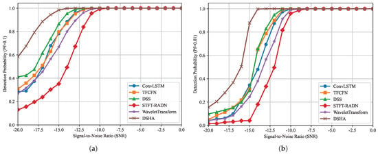
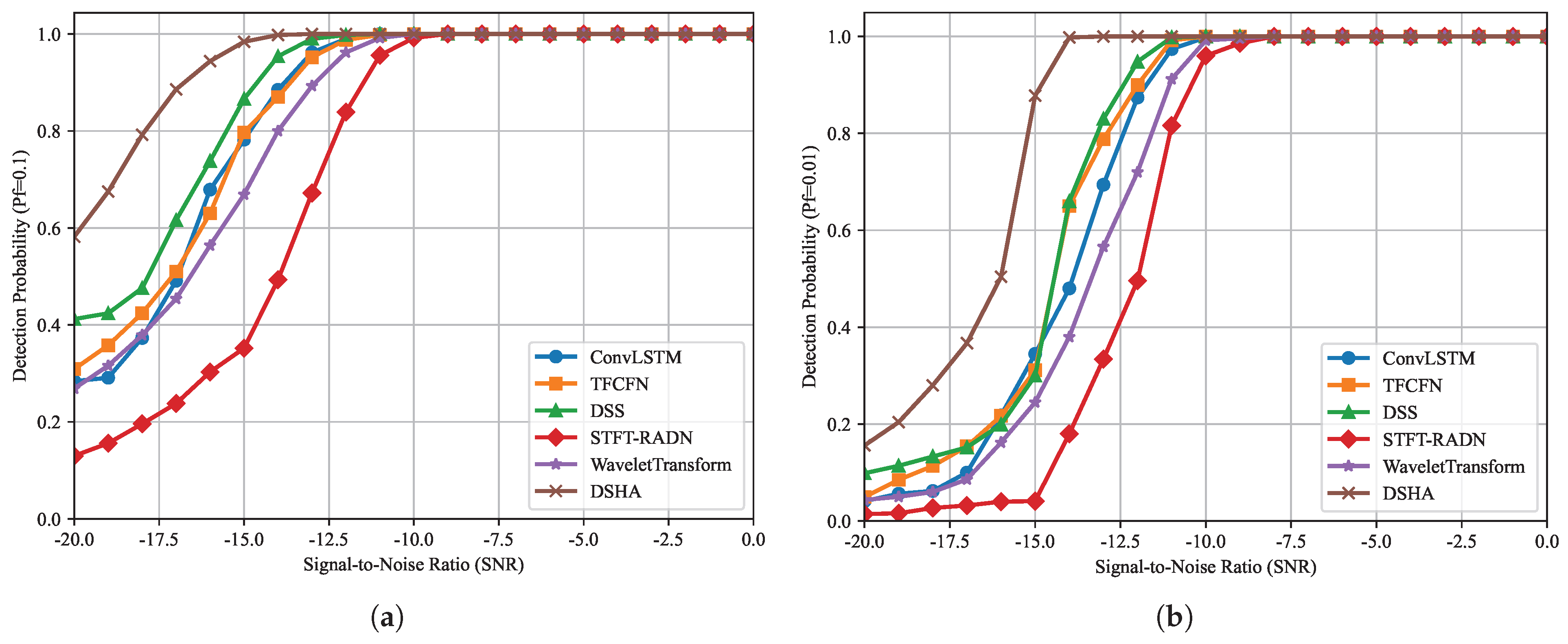
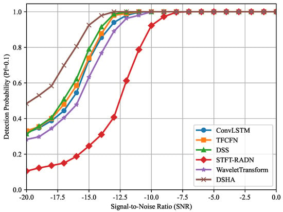
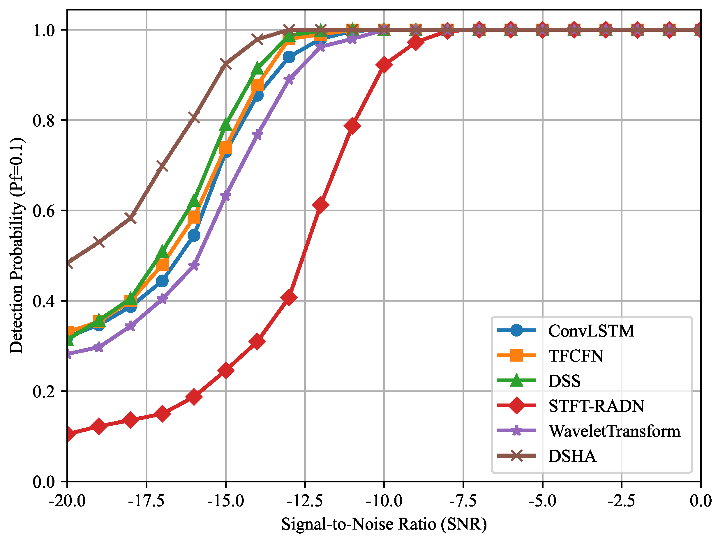
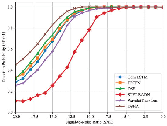
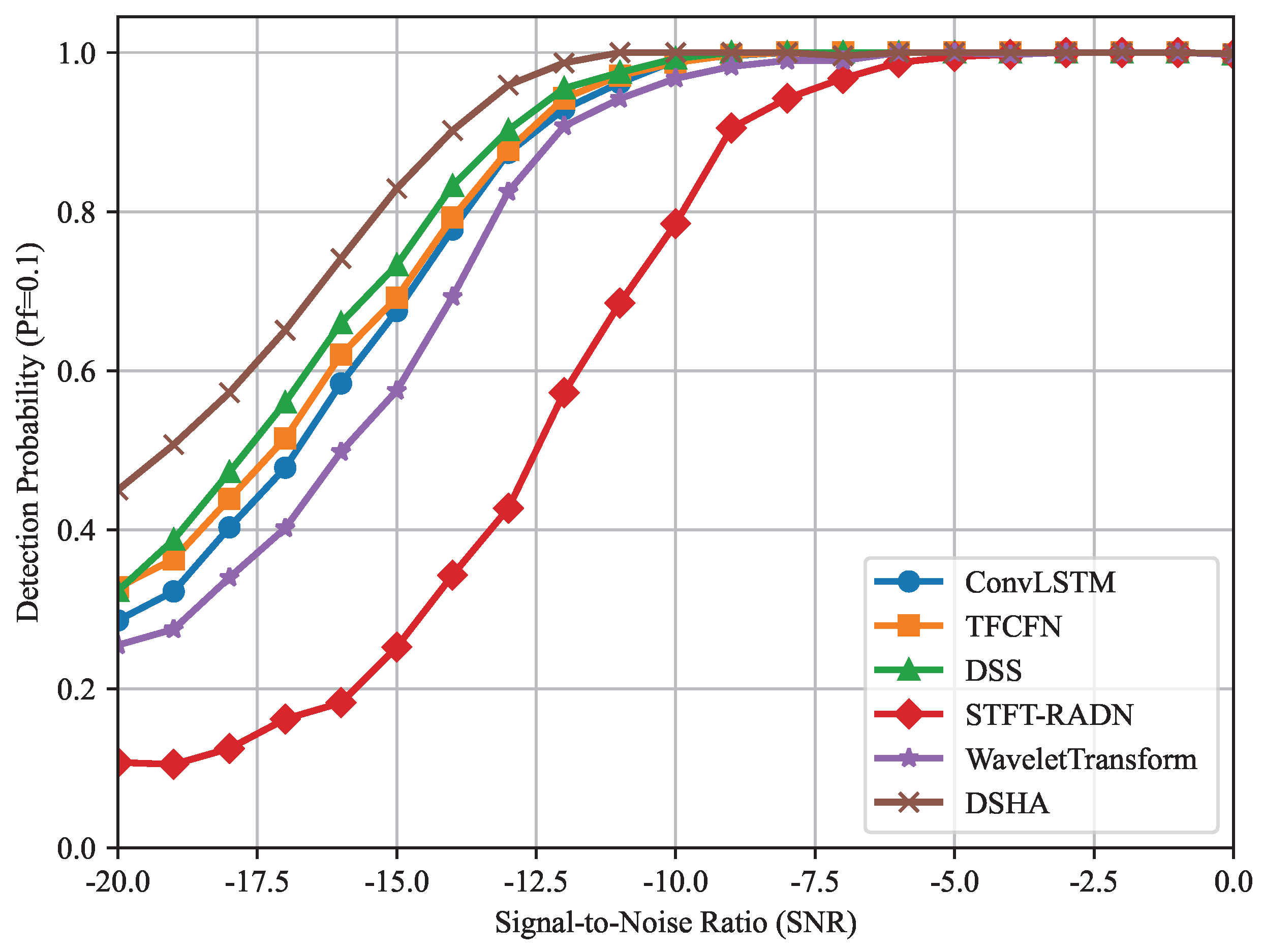
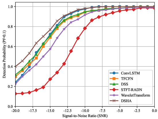
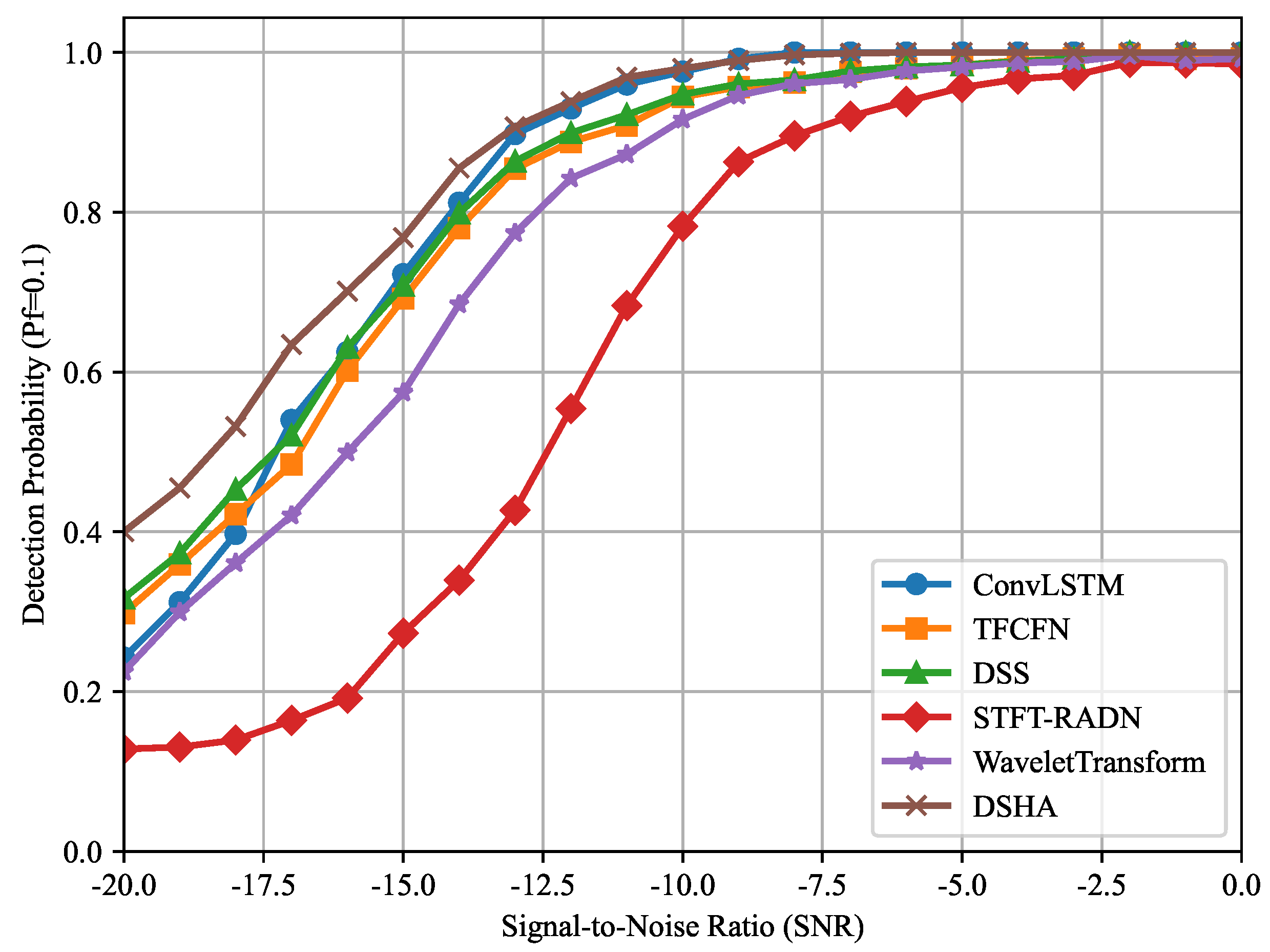
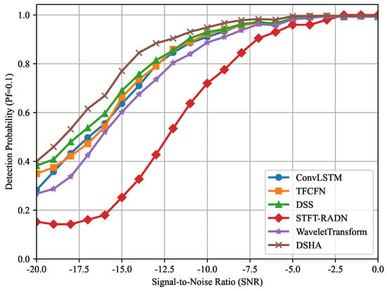
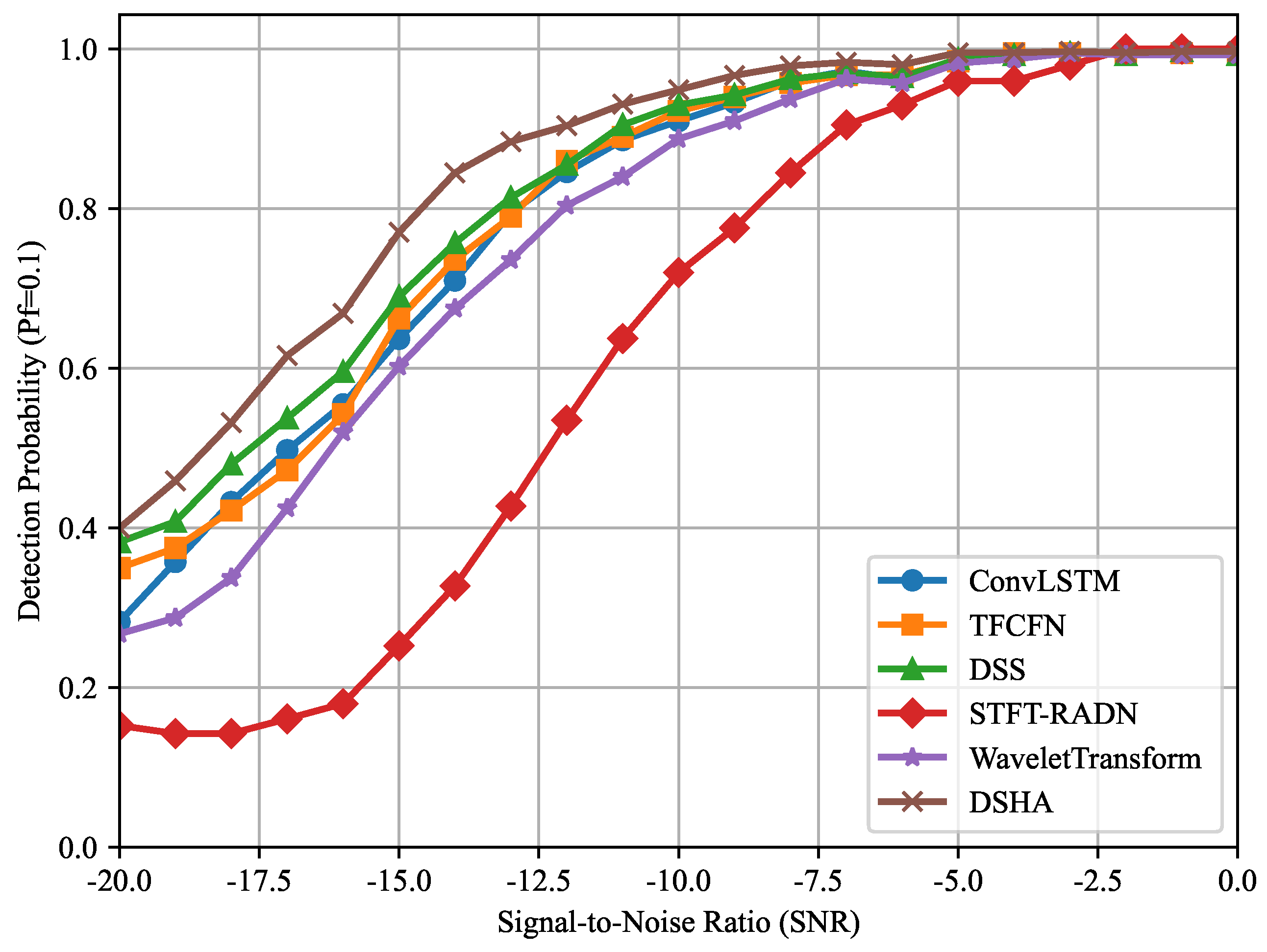
Figure 9 illustrates the $P_d$ versus SNR for different methods under two false-alarm probability settings, where Figure 9a and Figure 9b correspond to $P_f=0.1$ and $P_f=0.01$, respectively. As the SNR increases, $P_d$ rises for all methods and gradually approaches 1 in the high-SNR regime. The performance differences among these methods are mainly observed at low SNR. At the same SNR, the proposed DSHA method consistently achieves a higher $P_d$ than the other baselines, indicating stronger weak-signal detection capability and improved robustness.

Figure 9. Detection probabilities of different methods at two false-alarm probability levels. (a) Probability of detection of different approaches at $P_f$ = 0.1; (b) Probability of detection of different approaches at $P_f$ = 0.01.

Furthermore, Figure 9 shows that the proposed DSHA method requires a lower SNR than the other methods to achieve $P_d=1$. Specifically, when $P_f=0.1$, DSHA reaches $P_d=1$ at approximately −14 dB; when $P_f=0.01$, it requires approximately −13 dB. In contrast, among the baselines, the best-performing DSS method requires about −12 dB and −11 dB, respectively, to reach $P_d=1$, indicating an advantage of roughly 2 dB for DSHA. In addition, as $P_f$ decreases from 0.1 to 0.01, the curves for all methods shift to the right, suggesting that a higher SNR is needed to achieve the same $P_d$ under a stricter false-alarm constraint, which reflects the tradeoff between $P_f$ and $P_d$.

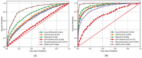
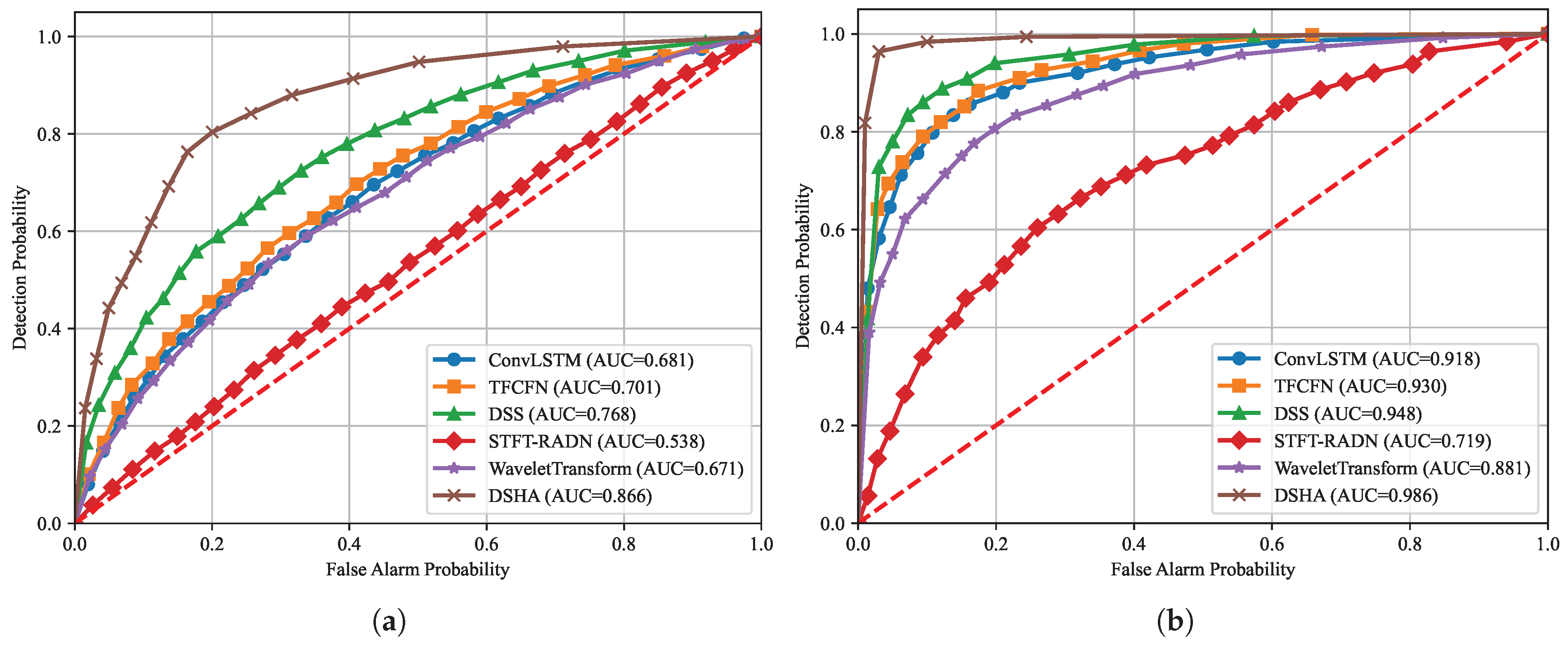
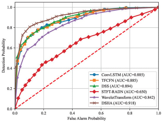
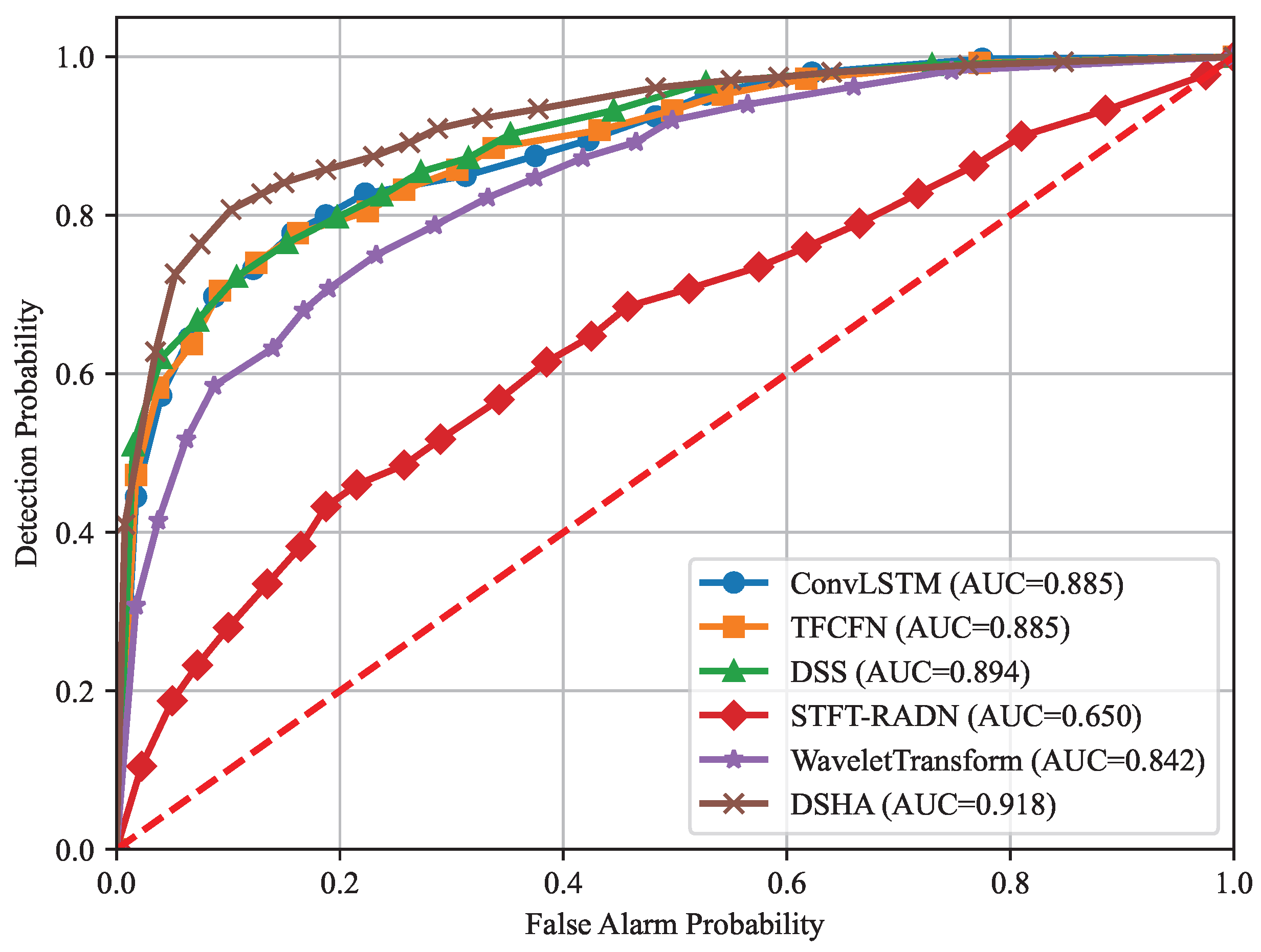
As the SNR decreases, the signal is gradually submerged in noise, which severely degrades spectrum sensing accuracy. To further evaluate performance in the low-SNR regime, we plot the ROC curves of all methods at SNR = −20 dB and SNR = −15 dB, as shown in Figure 10 The horizontal axis represents the false-alarm probability $P_f$, and the vertical axis denotes the detection probability $P_d$, thereby characterizing the tradeoff between $P_d$ and $P_f$ under different decision thresholds. A larger area under the curve indicates better performance. For quantitative comparison, we further adopt the area under the ROC curve (AUC) as an overall metric, and the AUC values of different methods at SNR = −20 dB and −15 dB are reported in Table 3. As shown in Figure 10 and Table 3, the proposed DSHA method achieves the highest AUC at both SNR levels, significantly outperforming the baseline methods, which indicates a stronger capability of discriminating between $H_1$ and $H_0$ under low-SNR conditions. Moreover, DSHA maintains a relatively high $P_d$ even at low $P_f$, further demonstrating its robustness to noise.

Figure 10. ROC curves of different methods at various SNR levels. (a) ROC curves at SNR = −20 dB; (b) ROC curves at SNR = −15 dB. The red dotted diagonal indicates random guessing performance, i.e., $P_d=P_f$.

Table 3. Comparison of AUC values of different methods at different SNR levels.

SNR	ConvLSTM	TFCFN	DSS	STFT-RADN	WaveletTransform	DSHA
$-15$ dB	0.918	0.930	0.948	0.719	0.881	0.986
$-20$ dB	0.681	0.701	0.768	0.538	0.671	0.866

5.2.2. Performance Under Rician Fading and Frequency Offset

The above results are obtained under the AWGN benchmark setting. Considering that LoS/NLoS fluctuations and mobility-induced frequency-offset perturbations in UAV air–ground links can significantly affect feature stability, we further evaluate the performance of all methods under Rician fading and frequency-offset conditions in this section.

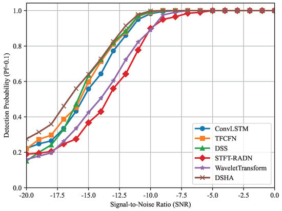
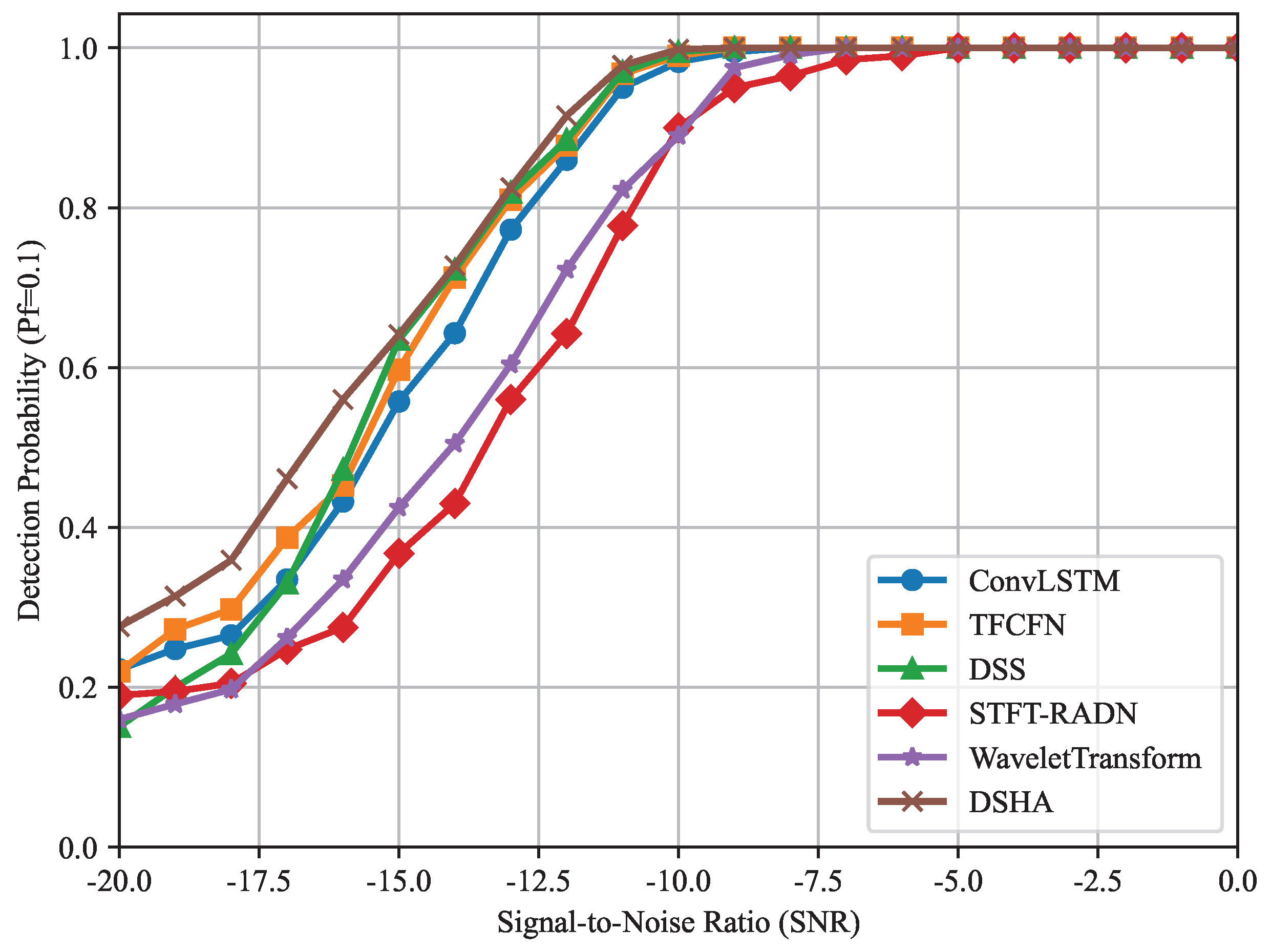
Figure 11 shows the $P_d$-SNR curves of different methods under Rician fading with (K = 20) and a fixed false-alarm probability $P_f=0.1$. As shown in Figure 11, as the SNR increases, the detection probability $P_d$ of all methods gradually increases and approaches 1 in the high-SNR region, indicating that reliable detection can be achieved. The DSHA curve lies above the competing methods overall and achieves a higher $P_d$ at the same SNR, demonstrating stronger weak-signal detection capability and better robustness under air–ground links with a strong LoS component.

Figure 11. $P_d$-SNR curves of the different methods under K = 20 and $P_f$ = 0.1.

Figure 12 shows the ROC curves of different methods at SNR = −15 dB with a Rician factor of K = 10. As shown in Figure 12, the ROC curve of DSHA lies above those of the competing methods overall, indicating that it achieves stronger separability between $H_1$ and $H_0$ and more robust threshold-dependent performance under the air–ground link condition.

Figure 12. ROC curves of different methods at SNR = −15 dB and K = 10. The red dotted diagonal indicates random guessing performance.

Figure 13 shows the $P_d$-SNR curves of different methods with $\epsilon =0.0005$ and $P_f$ = 0.1. As shown in Figure 13, performance degrades overall under Rician fading and frequency-offset perturbations, but DSHA remains the best performer in the low-SNR region, indicating stronger robustness to air–ground link variations and frequency-offset disturbances. DSHA reduces the SNR required to achieve $P_d\approx 1$ by about 1.5 dB compared with DSS. At SNR = −20 dB, the detection probability of DSHA is about 28.6% higher than that of DSS.

Figure 13. The $P_d$-SNR curves of different methods under $\epsilon =0.0005$ and $P_f=0.1$.

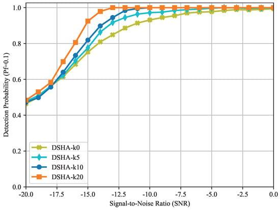
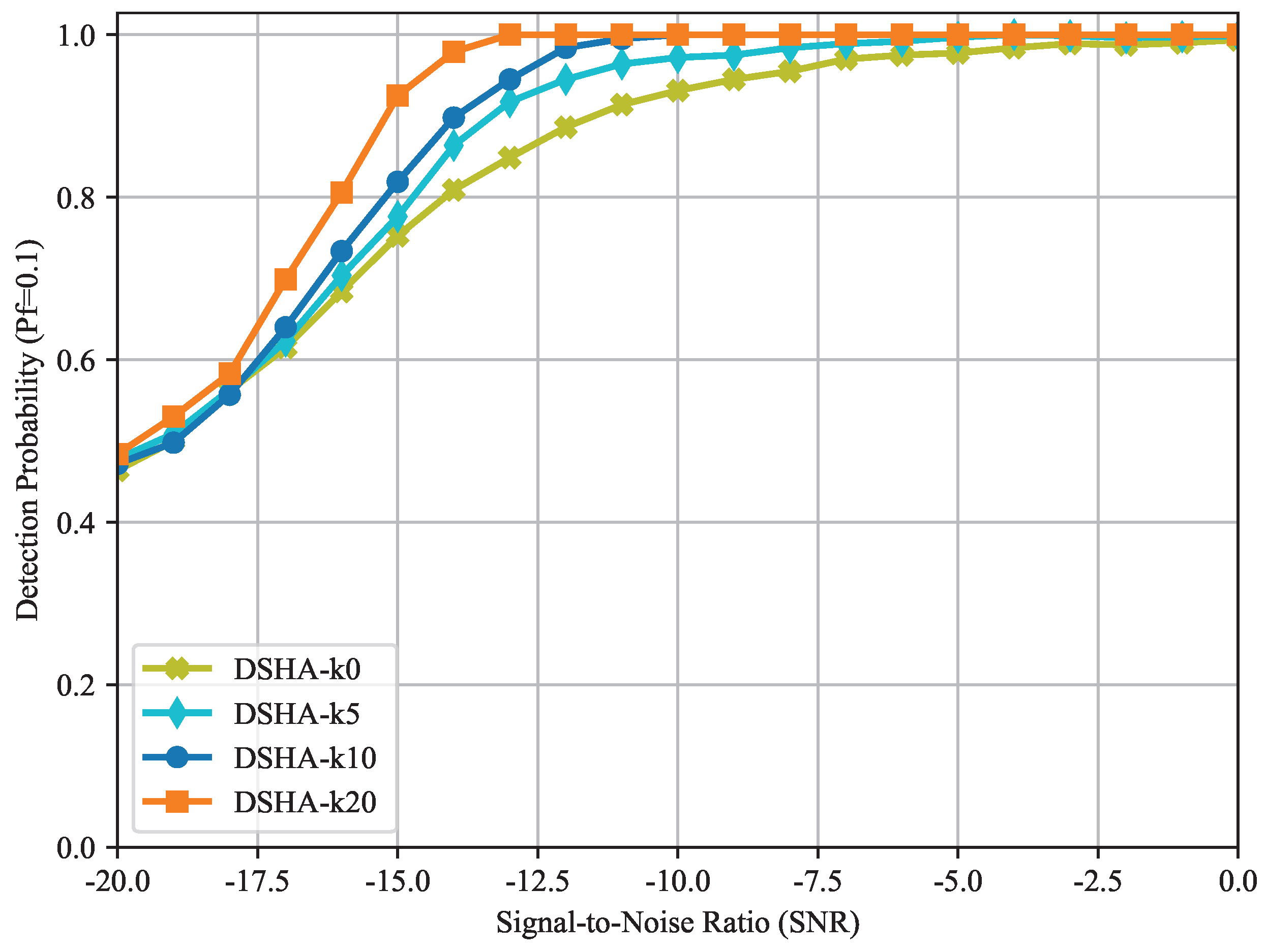
To further analyze the impact of LoS strength variations on DSHA, we sweep $K\in 0,5,10,20$. Figure 14 shows the $P_d$-SNR curves of DSHA under different K values with $P_f$ = 0.1. As shown in Figure 14, as K increases, the curves shift upward and approach $P_d$ = 1 more quickly. This indicates that DSHA exhibits a reasonable performance response to changes in LoS strength and maintains good detection stability over the tested range of K.

Figure 14. $P_d$-SNR curves of DSHA under different K values with $P_f$ = 0.1.

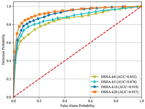
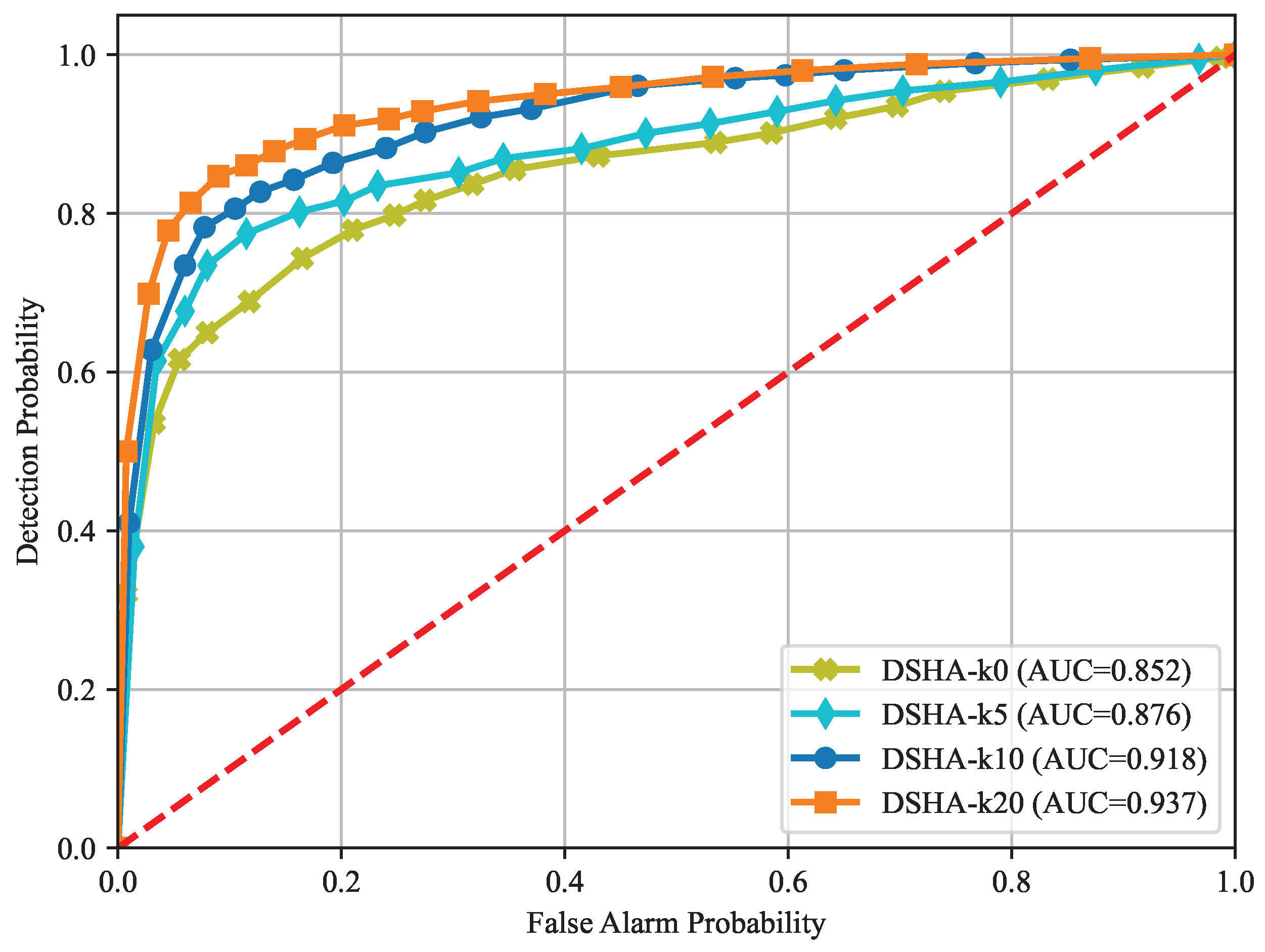
Figure 15 presents the ROC curves of DSHA under different K values and the corresponding AUC scores. As shown in Figure 15, with increasing K, the ROC curves move toward the upper-left corner, and the AUC increases monotonically from about 0.852 at K = 0 to about 0.937 at K = 20, consistent with the $P_d$-SNR results. This suggests that a stronger LoS component benefits detection performance, and DSHA maintains stable threshold-dependent performance across different LoS conditions.

Figure 15. ROC curves of DSHA under different K values with $P_f$ = 0.1. The red dotted diagonal indicates random guessing performance.

5.2.3. Robustness Evaluation Under Colored Noise

Figure 16 shows the $P_d$-SNR curves comparing the DSHA method with baseline methods under colored noise conditions. From Figure 16, it can be seen that the DSHA method still outperforms other baseline methods. As the SNR increases, the detection probability of all methods also gradually increases. However, the DSHA method exhibits stronger robustness at low SNR, demonstrating the effectiveness of the DSHA method in colored noise environments.

Figure 16. $P_d$-SNR curves of different methods under colored noise.

5.2.4. Frequency Offset Mismatch Results

To further evaluate the robustness of the NCPT-trained model under shifted conditions and its adaptability to unpaired data, we conduct a frequency offset experiment. During the training phase, we use paired data with different frequency offsets, where the frequency offset range is $ϵ\in \{0,0.0001,0.0005,0.001,0.005\}$. However, in the testing phase, we evaluate the model on unpaired test data, with the frequency offset set to $ϵ=0.0075$, which is outside the range of the training data. Figure 17 shows the $P_d$-SNR curves comparing the DSHA method and baseline methods under frequency offset mismatch.

Figure 17. $P_d$-SNR curves of different methods under frequency offset mismatch.

From Figure 17, it can be seen that even when the test frequency offset does not match the training frequency offset, the DSHA method still outperforms the baseline methods, although its performance is slightly lower compared to the case where the test and training frequency offsets are the same. It demonstrates the robustness and adaptability of our method under unpaired data and shifted conditions.

5.3. Ablation Study

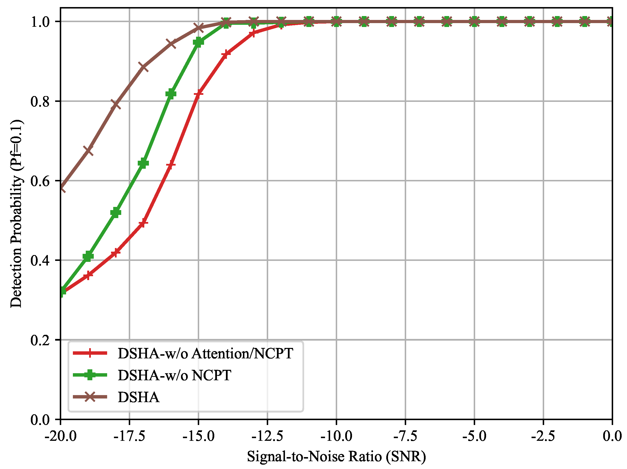
To evaluate the contribution of each component in the proposed DSHA spectrum sensing method, we further conduct ablation studies. Under a constant false-alarm probability of $P_f$ = 0.1, the $P_d$-SNR curves of different model variants are shown in Figure 18. Specifically, we compare (i) a dual-stream network without the attention mechanism and NCPT training (DualNet), (ii) a dual-stream network equipped with an attention mechanism (DualAttention), and (iii) DSHA, obtained by further introducing the noise-consistent paired training strategy based on DualAttention. All three variants are trained with the same training hyperparameters and training set composition.

Figure 18. $P_d$-SNR curves of DSHA variants at $P_f$ = 0.1.

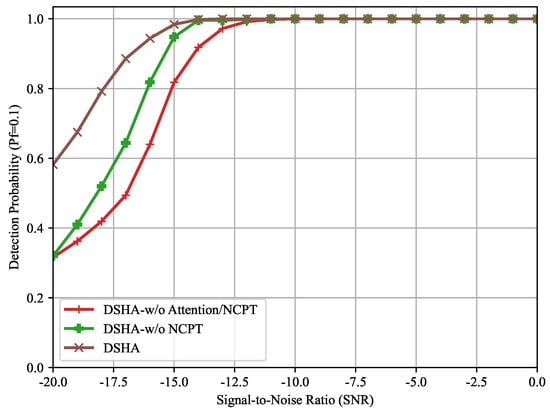
From Figure 18, it can be observed that the detection probability of all three models increases with SNR and gradually approaches 1 in the high-SNR regime. In the low-SNR regime, DualAttention achieves a markedly higher $P_d$ than DualNet at the same SNR, reaching $P_d$ = 1 at approximately −14 dB, whereas DualNet requires about −11 dB. It indicates that the attention mechanism can more effectively emphasize features associated with signal presence, thereby improving detection accuracy under low-SNR conditions. Moreover, DSHA provides a more pronounced gain. Its curve consistently lies above the others at low SNR. It suggests that noise-consistent paired training can alleviate the ambiguity between signal and noise characteristics in the low-SNR regime, enabling the model to learn representations that are less sensitive to noise perturbations and thus improving detection robustness. Overall, both the attention mechanism and the noise-aligned training strategy make clear contributions to performance improvement, and their combination significantly enhances detection accuracy under low-SNR conditions.

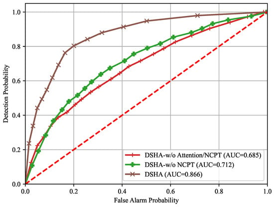
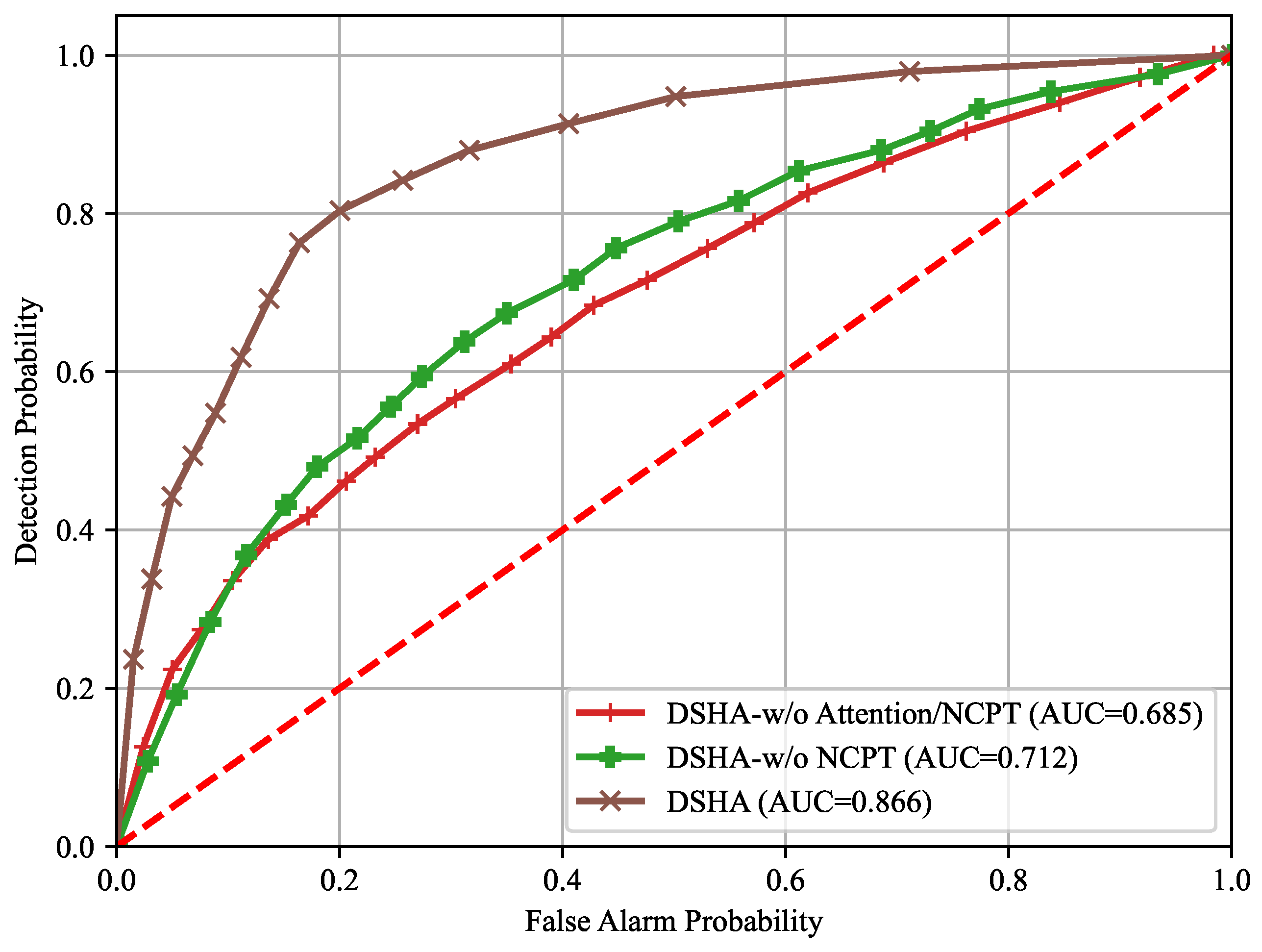
Figure 19 presents the ROC curves of the three variants at SNR = −20 dB, where the horizontal axis denotes $P_f$, and the vertical axis denotes $P_d$. It can be observed that DualAttention consistently outperforms DualNet, indicating that introducing the attention mechanism enhances discriminative features and improves separability at low SNR. Moreover, DSHA, which further incorporates noise-consistent paired training, achieves the best performance over the entire $P_f$ range. It also maintains a relatively high Pd in the low $P_f$ region, demonstrating stronger robustness in the low-SNR regime. For quantitative comparison, Table 4 summarizes the corresponding AUC values. DSHA attains an AUC of 0.866, which is significantly higher than those of DualAttention (0.712) and DualNet (0.685), further confirming that noise-consistent paired training enhances the separability between $H_1$ and $H_0$ at low SNR, thereby improving robustness in the low-SNR regime.

Figure 19. ROC curves of DSHA variants at SNR = −20 dB. The red dotted diagonal indicates random guessing performance.

Table 4. Comparison of AUC values of DSHA variants at SNR = −20 dB.

Model	DSHA	DualNet	DualAttention
AUC	0.866	0.685	0.712

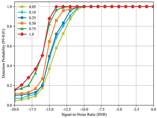
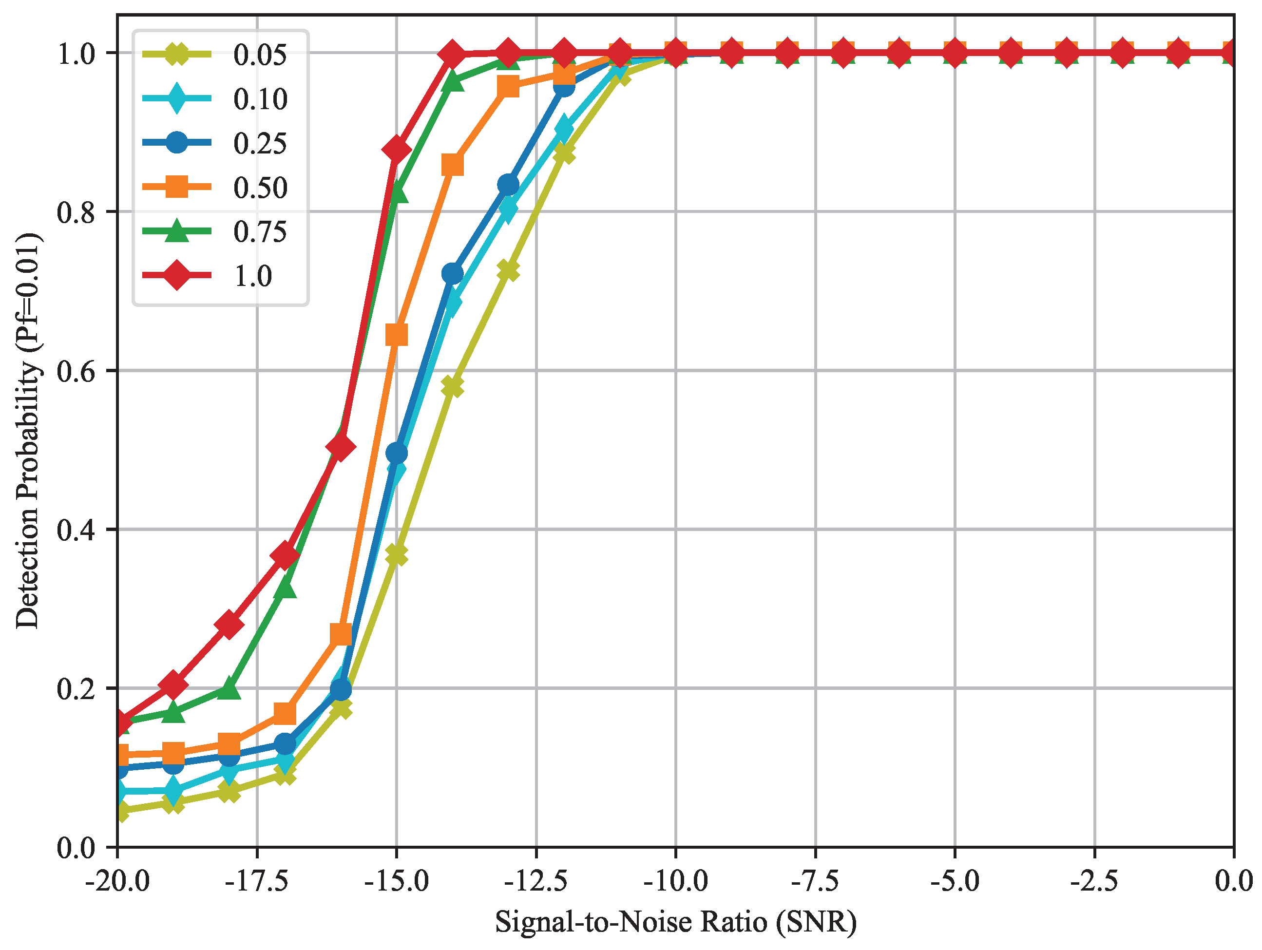
Moreover, to evaluate the impact of training set size on DSHA performance, we downsample the training set by different ratios. Specifically, 1.0 indicates that the full training set is used, whereas 0.75, 0.5, 0.25, 0.1, and 0.05 indicate that the corresponding fractions of the data are used for training. The resulting $P_d$-SNR curves at the fixed $P_f$ = 0.01 are shown in Figure 20. As the training data fraction decreases, the curves in the low-SNR region shift downward and exhibit a more pronounced rightward shift, meaning that $P_d$ is lower at the same SNR, and a higher SNR is required to achieve the same $P_d$. By contrast, in the high-SNR region, all curves gradually approach $P_d$ = 1, suggesting that the effect of training set size is mainly reflected in the noise-dominated low-SNR regime. It indicates that, when the number of training samples is insufficient, the ability of the model to learn and generalize signal-related features is constrained at low SNR. When a larger fraction of training data is used, the performance gap narrows noticeably, implying that DSHA learns more stably with sufficient data. Overall, increasing the training set size yields more pronounced gains at low SNR, whereas in the medium-to-high SNR regime, further improvements become relatively limited as performance saturates.

Figure 20. $P_d$-SNR curves under different training set sizes at $P_f$ = 0.01.

5.4. Over-the-Air Validation with an SDR Testbed

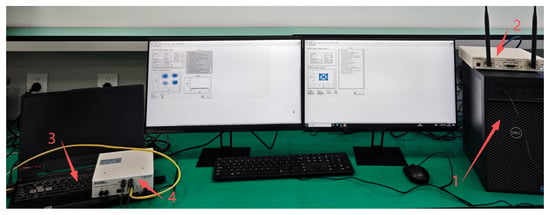
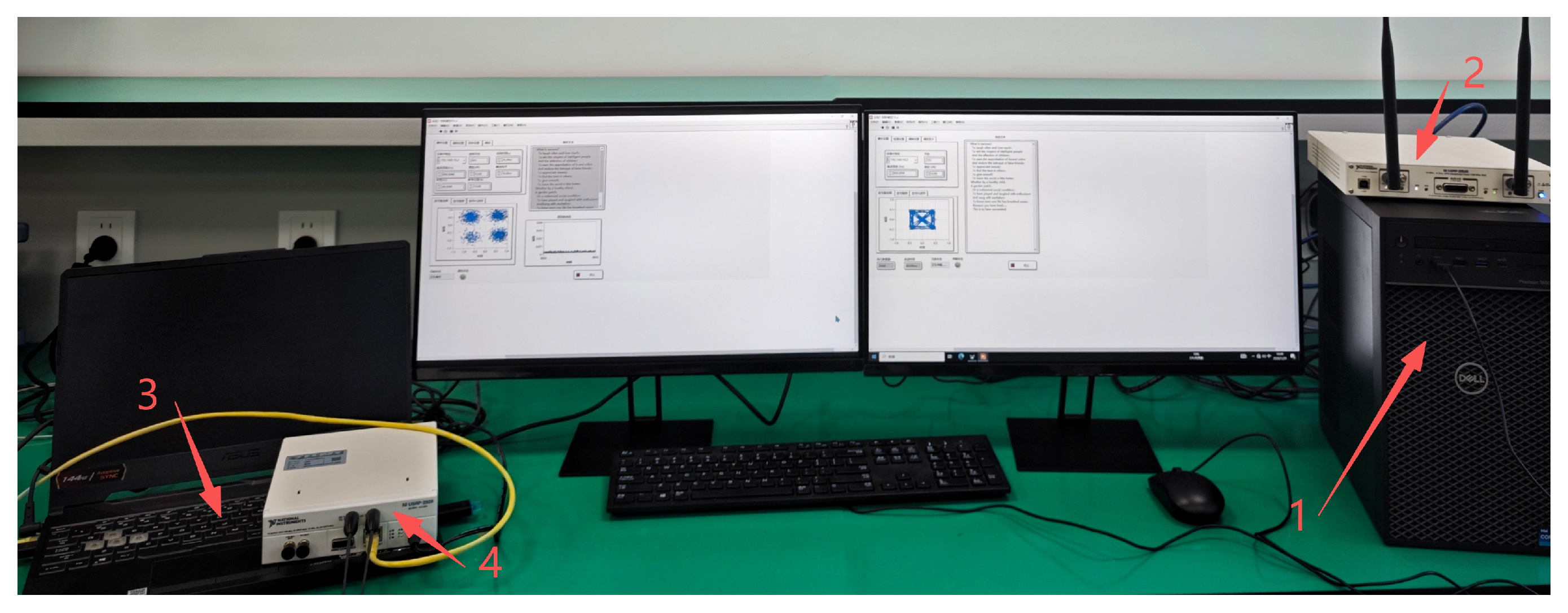
To validate the robustness of the proposed DSHA framework against real-world RF hardware imperfections and environmental factors, we built an indoor Over-the-Air (OTA) transmission and reception link based on Software-Defined Radio (SDR), as shown in Figure 21. The system consists of a host PC ((1) in Figure 21), which drives the USRP-2954R (2) for RF signal transmission. The receiver captures the OTA signal via the USRP-2920 (4), which is then connected to a laptop (3) for real-time signal processing and data analysis, allowing full transmission and reception of the signal with real-time monitoring. It should be noted that although the QPSK waveform used in this experiment is the same as that in the simulation, the transmission and reception process inherently introduces factors that are not fully captured by the synthetic AWGN and Rician channels, such as I/Q imbalance, quantization noise, and real multipath caused by indoor reflections. Therefore, the OTA platform can be used to validate the robustness of DSHA under practical real-world conditions.

Figure 21. Wireless transmission scenario diagram.

Figure 22 shows the performance comparison of the DSHA framework with the baseline methods on the real-world dataset. With a fixed false alarm probability of 0.1, it can be seen from the figure that the DSHA method still outperforms the other methods. However, due to environmental factors present in the real data, the performance is slightly lower compared to the simulation dataset.

Figure 22. Detection probability of different methods on the real-world dataset.

5.5. Network Performance and Computational Overhead Analysis

To further evaluate the feasibility of the proposed DSHA method, especially in practical applications such as UAV deployment, we report the parameter count, FLOPs, and inference latency of the model. These metrics help analyze the computational overhead of the method and reveal the impact of the Attention mechanism and dual-stream processing structure on performance. Table 5 presents a comparison of these computational metrics between the DSHA method and baseline methods. Specifically, DSHA w/o Attention, w/o STFT subnetwork refers to the model that neither includes the STFT branch nor the Attention mechanism, while DSHA w/o Attention refers to the model that excludes the Attention mechanism.

Table 5. Computational Metrics of DSHA Method and Baseline Methods.

Method	Parameter Count/M	Time Consumption (GPU/CPU)/ms	FLOPs/M
DSHA w/o Attention, w/o STFT sub network	0.821	2.53/4.37	70.96
DSHA w/o Attention	2.363	6.76/17.95	520.15
DSHA	5.639	9.56/45.7	628.24
ConvLSTM	0.132	9.32/7.40	2.59
TFCFN	0.0341	2.14/27.5	27.78
DSS	33.379	8.18/16.14	625.17
STFT-RADN	0.599	13.51/87.35	9.93
Wavelet Transformer	0.340	27.88/41.80	2.91

As shown in Table 5, compared to the baseline methods, the DSHA method has a higher parameter count and FLOPs, mainly due to the inclusion of STFT processing and the Attention mechanism. This results in an increase in the computational overhead of the model. In contrast, the baseline methods, which are based on 1D convolutional architectures with only a few fully connected layers, have relatively fewer parameters. The DSS method, being a fully connected network, has a significantly higher parameter count. However, due to the parallelism of our dual-stream network architecture, the inference speed of the DSHA method is comparable to that of the other methods when run on high-performance GPUs.

6. Conclusions

In this paper, we propose a deep-learning-based spectrum sensing method for UAV spectrum-sharing scenarios, termed DSHA. To address the limitations of existing methods that often rely on late-stage concatenation or simple fusion of multi-domain information and exhibit limited robustness under noise-dominant conditions, DSHA constructs two complementary inputs from the same received sequence, namely a time-domain I/Q sequence and an STFT magnitude spectrogram, and incorporates a hybrid-attention mechanism. Intra-branch self-attention is used to enhance key intra-domain dependency modeling, while inter-branch cross-attention enables explicit interaction and adaptive fusion between the time-domain and time-frequency-domain representations, thereby improving separability and detection performance under weak-signal conditions. In addition, we propose a noise-aligned paired training strategy (NCPT), which uses $H_1$ and $H_0$ sample pairs with shared noise realizations together with a paired constraint to guide the model to focus on occupancy-related differences while suppressing the influence of noise randomness. Experimental results show that DSHA outperforms multiple baseline methods under both the AWGN benchmark setting and more UAV-relevant conditions with Rician fading and normalized frequency-offset perturbations, with more pronounced gains in the low-SNR region. Moreover, ablation studies confirm that the hybrid-attention mechanism and NCPT effectively improve spectrum sensing performance under low-SNR conditions. In future work, we will further validate the proposed method under more realistic UAV air–ground communication settings by considering time-varying air–ground channels and mobility trajectories, interference coexistence and multi-user scenarios, and the combined effects of hardware impairments and synchronization errors, and we will explore lightweight deployment and online adaptation mechanisms to enhance generalization and real-time performance in complex environments.

References

- Mahmood, K.; Shamshad, S.; Anisi, M.H.; Brighente, A.; Saleem, M.A.; Das, A.K. A privacy-preserving access control protocol for 6G supported intelligent UAV networks. Veh. Commun. 2025, 54, 100937. [Google Scholar] [CrossRef] [Scilit]
- Zhang, G. 6G enabled UAV traffic management models using deep learning algorithms. Wirel. Netw. 2024, 30, 6709–6719. [Google Scholar] [CrossRef] [Scilit]
- Xia, X.; Xiang, N.; Zou, D.; Wang, D.; Zhao, Z. An Air-Ground Cooperative Situation Fusion Algorithm Based on Multi-unmanned Ground Vehicle and Multi-unmanned Aerial Vehicle. In International Conference on Autonomous Unmanned Systems; Springer: Singapore, 2024; pp. 454–467. [Google Scholar]
- Bennageh, I.; Mahmoudi, H.; Labbadi, M. Impact of the Electromagnetic Environment on UAV’s Datalink. In IOP Conference Series: Earth and Environmental Science; IOP Publishing: Bristol, UK, 2021; Volume 785, p. 012010. [Google Scholar]
- Gu, X.; Chen, G.; Wu, G.; Wen, C. Joint optimization of relay communication rates in clustered drones under interference conditions. Drones 2024, 8, 381. [Google Scholar] [CrossRef] [Scilit]
- Gonzalez, V.; Jaillet, P. Multi-drone rescue search in a large network. Eur. J. Oper. Res. 2025, 324, 787–798. [Google Scholar] [CrossRef] [Scilit]
- Du, J.; Wang, J.; Li, S.; Liu, L.; Chu, X.; Chen, X.; Dong, M. Intelligent Optimizations for UAV, Digital Twin, and ISCC Enabled Intelligent Transportation Systems. IEEE Trans. Intell. Transp. Syst. 2025, 26, 23069–23083. [Google Scholar] [CrossRef] [Scilit]
- Ye, C.; Zhu, W.; Guo, S.; Bai, J. DQN-Based Shaped Reward Function Mold for UAV Emergency Communication. Appl. Sci. 2024, 14, 10496. [Google Scholar] [CrossRef] [Scilit]
- Guimarães, D.A. Spectrum Hole Geolocation for Database-Driven IoT-Enabled Dynamic Spectrum Access. IEEE Access 2025, 13, 64199–64215. [Google Scholar] [CrossRef] [Scilit]
- Islam, A.M.; Rabbani, R.B.; Aadeeb, M.S.; Zareei, M.; Mansoor, N.; Zubaer, M.M. Simulation Tools for Cognitive Radio Network: A Survey. IEEE Access 2025, 13, 32384–32410. [Google Scholar] [CrossRef] [Scilit]
- Wang, S.; Huang, X.L.; Hu, F.; Yu, S. A Fast-Convergence, Induced Dynamic Spectrum Access Based on Accelerated Q-Learning for Cognitive Radio Networks. IEEE Trans. Veh. Technol. 2025, 74, 13925–13937. [Google Scholar] [CrossRef] [Scilit]
- Al-Matari, N.Y.; Zahary, A.T.; A. Al-Shargabi, A. A survey on advancements in blockchain-enabled spectrum access security for 6G cognitive radio IoT networks. Sci. Rep. 2024, 14, 30990. [Google Scholar] [CrossRef] [Scilit]
- Zhang, J.; Liang, C.L.; Gao, H.X.; Yan, H.; Zhu, H.B. Throughput-delay tradeoff for opportunistic spectrum access in cognitive radio networks. IET Commun. 2023, 17, 2053–2067. [Google Scholar] [CrossRef] [Scilit]
- Muzaffar, M.U.; Sharqi, R. A review of spectrum sensing in modern cognitive radio networks. Telecommun. Syst. 2024, 85, 347–363. [Google Scholar] [CrossRef] [Scilit]
- Saravanan, R.; Muthaiah, R.; Rajesh, A. Modified Black Widow Optimization-Based Enhanced Threshold Energy Detection Technique for Spectrum Sensing in Cognitive Radio Networks. CMES-Comput. Model. Eng. Sci. 2024, 138, 2339. [Google Scholar] [CrossRef] [Scilit]
- Saravanan, R.; Rajappa, M.; Amirtharajan, R. Modified Gannet Optimization Algorithm Based Enhanced Entropy Energy Detection Technique for Spectrum Sensing in Cognitive Radio Networks. Wirel. Pers. Commun. 2025, 140, 833–852. [Google Scholar] [CrossRef] [Scilit]
- Brito, A.; Sebastião, P.; Velez, F.J. Hybrid matched filter detection spectrum sensing. IEEE Access 2021, 9, 165504–165516. [Google Scholar] [CrossRef] [Scilit]
- Zhang, C.; Li, J.; Li, B.; Ma, W. Blind matching filtering algorithm for spectrum sensing under multi-path channel environment. Electronics 2023, 12, 2499. [Google Scholar] [CrossRef] [Scilit]
- Labsis, L.; Teguig, D.; Lassami, N.; Touami, H.C. An advanced blind cyclostationary spectrum sensing algorithm for cognitive radio networks. Phys. Scr. 2025, 100, 065502. [Google Scholar] [CrossRef] [Scilit]
- Ni, T.; Ding, X.; Wang, Y.; Shen, J.; Jiang, L.; Zhang, G. Spectrum sensing via temporal convolutional network. China Commun. 2021, 18, 37–47. [Google Scholar] [CrossRef] [Scilit]
- Gai, J.; Xue, X.; Li, Z.; Zhang, L. Spectrum sensing method based on residual cellular network. IEEE Access 2022, 10, 61354–61365. [Google Scholar] [CrossRef] [Scilit]
- Mehrabian, A.; Sabbaghian, M.; Yanikomeroglu, H. CNN-based detector for spectrum sensing with general noise models. IEEE Trans. Wirel. Commun. 2022, 22, 1235–1249. [Google Scholar] [CrossRef] [Scilit]
- Wang, Q.; Su, B.; Wang, C.; Qian, L.P.; Wu, Y.; Yang, X. ConvLSTM-based spectrum sensing at very low SNR. IEEE Wirel. Commun. Lett. 2023, 12, 967–971. [Google Scholar] [CrossRef] [Scilit]
- Mondal, S.; Dutta, M.P.; Chakraborty, S.K. A hybrid deep learning based approach for spectrum sensing in cognitive radio. Phys. Commun. 2024, 67, 102497. [Google Scholar] [CrossRef] [Scilit]
- Xing, H.; Qin, H.; Luo, S.; Dai, P.; Xu, L.; Cheng, X. Spectrum sensing in cognitive radio: A deep learning based model. Trans. Emerg. Telecommun. Technol. 2022, 33, e4388. [Google Scholar] [CrossRef] [Scilit]
- Vijay, E.V.; Aparna, K. Spectrum sensing using deep learning for proficient data transmission in wireless sensor networks for wireless communication. Ain Shams Eng. J. 2024, 15, 102784. [Google Scholar] [CrossRef] [Scilit]
- Liu, C.; Wang, J.; Liu, X.; Liang, Y.C. Deep CM-CNN for spectrum sensing in cognitive radio. IEEE J. Sel. Areas Commun. 2019, 37, 2306–2321. [Google Scholar] [CrossRef] [Scilit]
- Xie, J.; Fang, J.; Liu, C.; Li, X. Deep learning-based spectrum sensing in cognitive radio: A CNN-LSTM approach. IEEE Commun. Lett. 2020, 24, 2196–2200. [Google Scholar] [CrossRef] [Scilit]
- Chen, W.; Wu, H.; Ren, S. Cm-lstm based spectrum sensing. Sensors 2022, 22, 2286. [Google Scholar] [CrossRef] [Scilit]
- Chae, K.; Park, J.; Kim, Y. Rethinking autocorrelation for deep spectrum sensing in cognitive radio networks. IEEE Internet Things J. 2022, 10, 31–41. [Google Scholar] [CrossRef] [Scilit]
- Zhen, P.; Zhang, B.; Chen, Z.; Guo, D.; Ma, W. Spectrum sensing method based on wavelet transform and residual network. IEEE Wirel. Commun. Lett. 2022, 11, 2517–2521. [Google Scholar] [CrossRef] [Scilit]
- Zhao, S.; Xue, W.; Xu, Y. Deep CWT-ResLSTM for spectrum sensing in cognitive radio. Signal Image Video Process. 2025, 19, 531. [Google Scholar] [CrossRef] [Scilit]
- Chen, Z.; Xu, Y.Q.; Wang, H.; Guo, D. Deep STFT-CNN for spectrum sensing in cognitive radio. IEEE Commun. Lett. 2020, 25, 864–868. [Google Scholar] [CrossRef] [Scilit]
- Gai, J.; Zhang, L.; Wei, Z. Spectrum sensing based on STFT-ImpResNet for cognitive radio. Electronics 2022, 11, 2437. [Google Scholar] [CrossRef] [Scilit]
- Wang, A.; Zhu, T.; Meng, Q. Spectrum sensing method based on STFT-RADN in cognitive radio networks. Sensors 2024, 24, 5792. [Google Scholar] [CrossRef] [Scilit]
- Zhang, Y.; Luo, Z. A deep-learning-based method for spectrum sensing with multiple feature combination. Electronics 2024, 13, 2705. [Google Scholar] [CrossRef] [Scilit]
- Bai, X.; Xu, J.; Fang, F.; Wang, X.; Wang, S. A Multi-Feature Spectrum Sensing Algorithm Based on GRU-AM. IEEE Wirel. Commun. Lett. 2025, 14, 2129–2133. [Google Scholar] [CrossRef] [Scilit]
- Wang, A.; Meng, Q.; Wang, M. Spectrum sensing method based on residual dense network and attention. Sensors 2023, 23, 7791. [Google Scholar] [CrossRef] [Scilit] [PubMed]
- Xu, T.; Wang, Y.; Yan, M.; Liang, Q. Deep Learning-Based Spectrum Sensing with Fused Time-Frequency Representations. IEEE Commun. Lett. 2025, 29, 2386–2390. [Google Scholar] [CrossRef] [Scilit]
- Xi, H.; Guo, W.; Yang, Y.; Yuan, R.; Ma, H. Cross-attention mechanism-based spectrum sensing in generalized Gaussian noise. Sci. Rep. 2024, 14, 23261. [Google Scholar] [CrossRef] [Scilit] [PubMed]
Disclaimer/Publisher’s Note: The statements, opinions and data contained in all publications are solely those of the individual author(s) and contributor(s) and not of MDPI and/or the editor(s). MDPI and/or the editor(s) disclaim responsibility for any injury to people or property resulting from any ideas, methods, instructions or products referred to in the content. |
© 2026 by the authors. Licensee MDPI, Basel, Switzerland. This article is an open access article distributed under the terms and conditions of the Creative Commons Attribution (CC BY) license.