


Abstract
Data centers consumed 415 TWh of electricity in 2024, about 1.5% of global demand, and foundation model training and inference are a growing part of this load. As training and inference continue to grow, energy-efficient foundation models are becoming essential. An efficiency gain may come from the model, the accelerator, or the facility, and existing reviews and primary studies usually address one of these aspects. However, energy is obtained by a different method at each of these stages, so unified and systematic optimization is more difficult than results at any single stage may suggest. Reported metrics range from floating-point operations (FLOPs) and tera-operations per second per watt (TOPS/W) to throughput, power usage effectiveness (PUE), carbon, and water. This review follows energy through each stage and treats each reported value together with its measurement boundary and evidence class. This review covers the chain from how models are designed, compressed, and served through how accelerators execute them at reduced precision to how facilities cool and power them. This review identifies open research problems in wall-plug measurement, cross-layer co-design, lifecycle accounting, and the deployment maturity of emerging accelerators. It aims to serve as a reference for researchers and practitioners seeking a unified view of energy, carbon, and water across foundation model systems.
1. Introduction
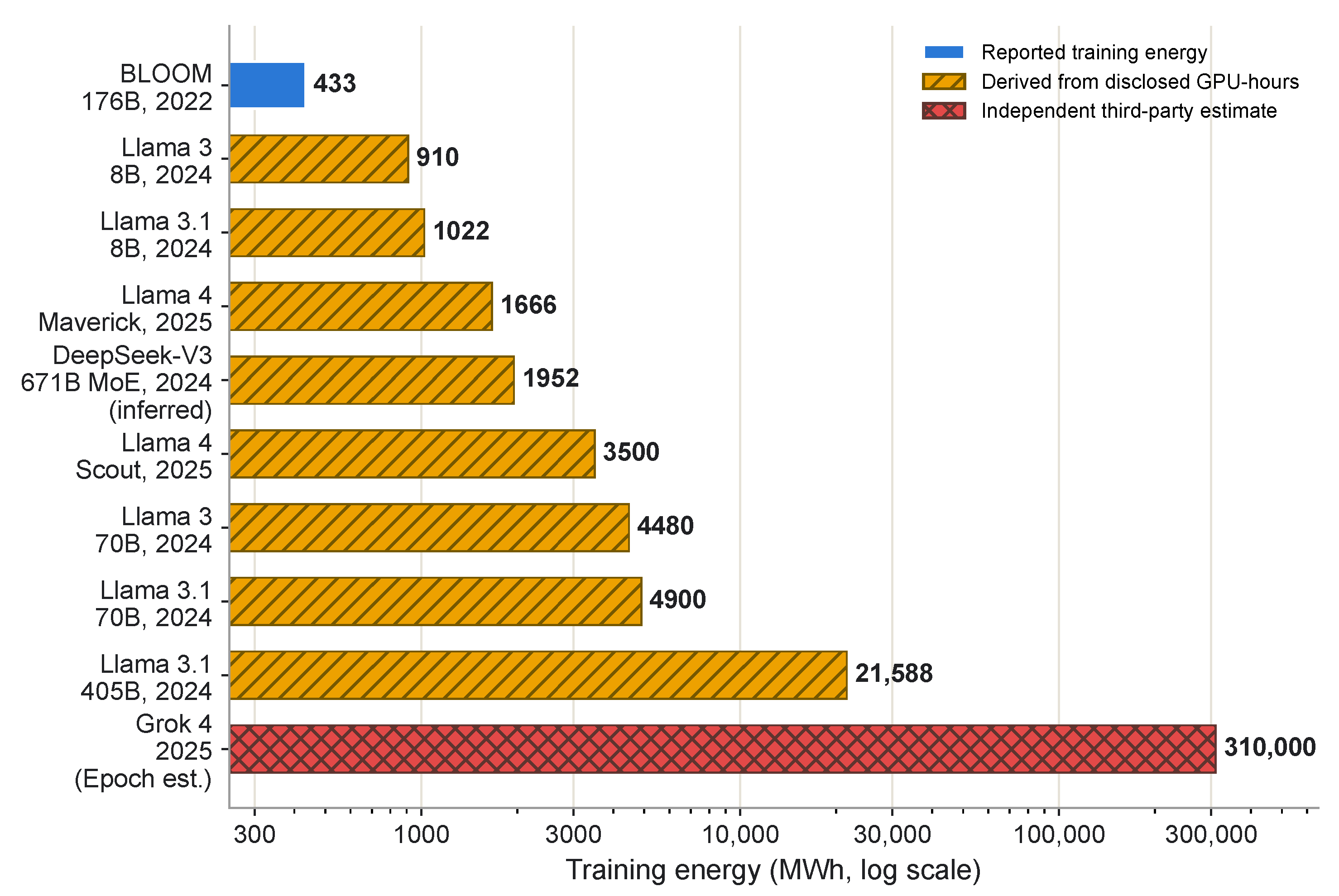
Data centers consumed 415 TWh of electricity in 2024, about 1.5% of global demand, and international projections anticipate continued growth through 2030 [1,2]. Energy use has become a design constraint for foundation models, and a gain made at one point in the system does not always lower what the facility finally draws. The compute used to train prominent artificial intelligence (AI) models has grown by orders of magnitude over the past decade. For selected milestone systems, an OpenAI analysis documented a more than 300,000× increase in training compute between 2012 and 2018 [3]. The shift from AlexNet-scale models to transformer-based systems [4] and then to large language models (LLMs) has made training and serving energy a practical constraint rather than a background cost. Officially disclosed data remain sparse, but available model team reports already show the scale of modern pretraining. BLOOM’s authors report 433,196 kWh for final training, while Meta model cards disclose 39.3 million H100 graphics processing unit (GPU) hours for the Llama 3.1 family, including 30.84 million GPU-hours for Llama 3.1 405B alone [5,6]. Using disclosed GPU-hours and a 700 W H100 accelerator-power assumption, this review derives an estimate of approximately 21,588 MWh for Llama 3.1 405B training; the conversion excludes host, network, and facility energy [7]. For systems without comparable official energy disclosure, carefully labeled estimates can still provide useful scale. DeepSeek-V3 reports 2.788 million H800 GPU-hours but not training electricity, while Epoch AI estimates Grok 4 training electricity at 310 GWh [8,9]. Such values are informative only when their estimation status and accounting boundary are explicit. Figure 1 collects these training energy values and labels each by evidence class.
Training remains the most visible stage, but inference is repeated continuously after deployment and can account for a large share of lifetime machine learning energy use under some accounting boundaries [10,11]. Other stages of model development and experimentation are less frequently measured despite their contribution to the total lifecycle footprint [12].
Research on reducing AI energy use now spans several communities. Model work studies efficient architectures, pruning, quantization, distillation, parameter-efficient fine-tuning, and serving systems [13,14]. Hardware research develops accelerators, memory systems, low-precision data paths, and near-memory or non-von Neumann architectures. Infrastructure research covers cooling, power delivery, energy procurement, workload placement, and grid-aware scheduling. However, the literature on these topics often optimizes different properties and reports different metrics. For instance, papers on algorithms typically report floating-point operations (FLOPs) or parameter count, hardware papers commonly report peak tera-operations per second per watt (TOPS/W), and data center reports emphasize power usage effectiveness (PUE) or energy procurement. These metrics are useful in context, but cannot individually establish the energy, carbon, or water impact of a deployed AI service. A model that halves FLOPs may not save energy if the target hardware cannot exploit the resulting sparsity pattern; likewise, a nominal improvement in accelerator TOPS/W may yield little carbon reduction when facility overhead or grid carbon intensity dominates the deployment boundary. This disconnect between local improvements and system-level outcomes makes it difficult for practitioners to determine which efficiency gains will survive deployment. Two challenges in energy-efficient AI follow. First, an efficiency gain may come from the model, from the accelerator, or from the facility, and existing reviews and primary studies usually address only one of those aspects. Second, energy is obtained by a different method at each stage, so unified and systematic optimization is harder than any result focusing on just one of the above aspects might suggest.
Green AI has been surveyed at different depths: Verdecchia et al. [15] mapped software techniques, Khan et al. [11] reviewed methods across algorithms, hardware, and infrastructure, and Desislavov et al. [16] tracked compute and energy trends across hardware generations. These three reviews differ in scope as well as in what they admit as evidence. The first works from software-level techniques; the second collects results across algorithms, hardware, and infrastructure; and the third follows trends over successive hardware generations rather than individual interventions. This review covers the same three areas as the second review while also adding the provenance of each reported value. This approach means that operator measurements, figures derived from disclosed GPU hours, modeled estimates, and vendor specifications are all distinguished when they are compared. If the system boundary changes, the accounts are no longer comparable because the energy use makes up a single chain: algorithms decide what is computed, hardware sets the cost of each operation and memory access, and the facility adds cooling, power delivery, water, and grid carbon overhead. Thus, an improvement at one layer represents measurable savings only if the neighboring layers do not offset it. This paper follows the aforementioned chain for foundation model workloads from model design through hardware and data center operation.
Figure 1.
Training energy for selected large language models, separated by evidence class. The blue BLOOM bar is model team-reported training electricity [5]. Yellow hatched bars are derived estimates that multiply the GPU hours disclosed in the Llama model cards [6,17,18] and the DeepSeek-V3 report [8] by the 700 W H100 thermal design power at which Meta reports having run its GPUs [7,19], a value also applied as an assumption to the H800 GPUs of DeepSeek-V3; they exclude host, network, and facility energy. The red cross-hatched Grok 4 bar is Epoch AI’s independent estimate [9]. DeepSeek-V3 and the Llama-family values should not be read as operator-disclosed wall-plug measurements. The log-scale axis supports comparison across model sizes, not full lifecycle energy.
The contribution of this review is to collect the quantitative evidence on energy, carbon, and water usage in foundation model systems and to present each value with the boundary at which it was obtained and the kind of evidence behind it. Unlike reviews organized around techniques alone, this review is organized around both the techniques and the provenance of the effects reported for them. Algorithmic efficiency covers efficient architectures, compression, fine-tuning, and decoding with key–value (KV) cache management. Hardware efficiency includes reduced precision, memory locality, and near-memory, neuromorphic, and photonic designs. Infrastructure efficiency extends to cooling, power delivery, renewable procurement, and workload scheduling. Across the three areas, the same pattern recurs: a reduction in computation or data movement lowers consumption only when the hardware and facility both preserve it, and a gain reported at one point is frequently offset elsewhere in the system. This review aims to serve as a resource for researchers and practitioners who work in one of these areas and need a basis for judging results reported in the other two.
2. System Boundaries and Metrics
As noted in Section 1, existing surveys cover complementary aspects of AI energy efficiency. This section reviews energy consumption across the AI lifecycle, the relationships among system layers, and the metrics that link model-level improvements to facility-level environmental outcomes.
2.1. Energy Consumption Across the AI Lifecycle
Energy optimization in machine learning usually targets training and inference, but other lifecycle stages can also affect total consumption. Preprocessing steps such as data cleaning, feature engineering, and exploratory analysis are rarely profiled for energy. Library choice alone (Pandas vs. Vaex vs. Dask) can alter energy use for identical operations by up to 202× [20]. Data-centric modifications such as reducing dataset size or feature count have reported energy reductions of up to 92% with limited accuracy loss [21], and in energy forecasting, preprocessing choices directly affect both cost and predictive quality [22]. Preprocessing can also be included in lifecycle measurements rather than being treated as negligible overhead.
Training, especially large-scale pretraining, dominates public attention. As noted in Section 1, compute requirements have grown by orders of magnitude over the past decade, and large-scale neural network training can impose substantial energy and carbon costs if hardware, data center efficiency, and grid mix are not reported [23,24]. Scaling-law research has shown that many LLMs are undertrained relative to their size, and that better data–model balance can match or exceed performance with less compute [25]. Parameter-efficient fine-tuning offers a separate route to training efficiency. Adapters [26] and low-rank adaptation (LoRA) [13] update only small additional or low-rank parameter sets, and quantized LoRA (QLoRA) combines 4-bit quantization with low-rank adapters to fine-tune 65B-parameter models on a single GPU [14]. One training stage that is less frequently accounted for in energy analyses is alignment through reinforcement learning from human feedback (RLHF). RLHF requires training a separate reward model and running multiple rounds of policy optimization, but quantitative energy data for this phase remain scarce.
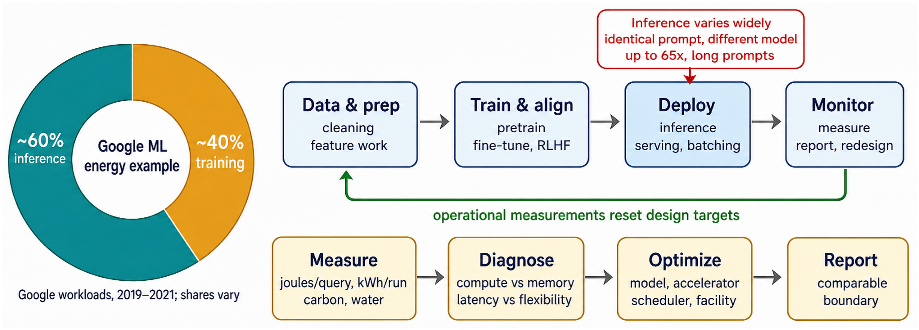
In deployment, energy costs can compound because inference runs continuously when systems are served at scale. Provider case studies report large reductions in energy and CO2e for selected workloads when model choice, hardware, data center siting, and workload scheduling are co-optimized [24]. Widespread AI integration into enterprise workflows can also increase cumulative demand [1,27]. Figure 2 maps this lifecycle so as to locate the energy within it. Preprocessing, training, and alignment are incurred per training run, whereas deployment is re-entered on every query, so the stage that is easiest to leave unmeasured is the one that accumulates energy for as long as the model is served. Inference accordingly accounted for roughly three-fifths of energy use in the sampled hyperscaler workloads [10,11], and per-query inference energy can vary by more than 65× across models under long-prompt settings [28]. In practice, the bottleneck is often data movement rather than arithmetic. In transformer training, memory access dominates runtime [29].
2.2. Layered View of Energy-Efficient AI
The techniques discussed below are organized by intervention layer rather than by model family or benchmark task. This descriptive grouping separates where a change is introduced from the system boundary at which impacts are finally counted. Energy traverses the stack from algorithm to hardware to facility. Computational demand originates in the model and serving configuration, is delivered through processor and memory subsystems, and is amplified by cooling, conversion losses, and grid exposure at the data center. The difficulty is that a local efficiency gain at one layer does not guarantee savings in production unless the change propagates favorably through the rest of the stack.
- Algorithmic Efficiency (Section 3). Methods that lower computational cost through model design, compression, training optimization, and serving, ranging from efficient architectures and pruning through quantization, distillation, and parameter-efficient fine-tuning to decoding, KV-cache management, and harness policies that control model routing, context use, tools, verification, and retries.
- Hardware Efficiency (Section 4). Processor and memory innovations that raise performance per watt, together with lower-precision data paths and emerging accelerators for processing-in-memory, neuromorphic, photonic, and quantum or hybrid computing.
- Infrastructure Efficiency (Section 5). Data center measures that reduce overhead from cooling and power delivery while improving renewable procurement and workload scheduling.
Figure 2.
AI lifecycle energy boundary for foundation model systems. The diagram separates preprocessing, training and alignment, deployment, monitoring, measurement, diagnosis, optimization, and reporting. A hyperscaler case study found that inference accounted for roughly three-fifths of Google ML energy use during sampled 2019–2021 workloads [10,11], but the training–inference split varies with workload, deployment scale, and retraining cadence. Preprocessing and alignment are often underreported, and Jegham et al. [28] estimate that per-query inference energy can vary by more than 65× across models under long-prompt settings.
These layers are interdependent. Algorithmic savings materialize most clearly when hardware can exploit sparsity or reduced precision, and facility infrastructure still governs the overhead that surrounds both.
2.3. Energy, Carbon, and Water Metrics
Several metrics are commonly used to quantify the energy efficiency and environmental impact of AI systems:
- FLOPs and FLOPs/Watt. Floating-point operations are commonly used as a proxy for computational workload, while FLOPs per watt relates that workload to hardware energy efficiency [16,30].
- Power Usage Effectiveness (PUE). Defined as total facility energy divided by IT equipment energy, PUE quantifies data center overhead [31]. It should be reported with the facility boundary and measurement period because operating conditions vary across sites.
- Water Usage Effectiveness (WUE). Defined as annual site water use divided by IT equipment energy, WUE relates facility water consumption to the computing load. It should be reported with the cooling method, site conditions, and water accounting boundary because identical requests can have different water footprints across facilities [28].
- Carbon Intensity. Carbon intensity measures CO2 emissions per unit of electricity or computation, linking model energy use to the grid mix used during training or inference [12,32].
- Performance per Watt. Per-watt performance evaluation relates task performance, throughput, or accuracy to energy consumption, and is central to Green AI reporting [30,33].
For example, a model that achieves 1% higher accuracy but consumes 10× more energy per query would appear superior under accuracy-only evaluation but would become untenable at deployment scale. Luccioni et al. documented the broader problem when comparing generative and task-specific models [33]. This mismatch motivates a shift from accuracy-centric evaluation towards per-watt performance metrics [30]. None of these metrics, however, is interchangeable with another. FLOPs and parameter counts are useful proxies for algorithmic cost, but do not capture memory traffic, hardware utilization, cooling overhead, water usage, or grid carbon intensity. Conversely, facility-level metrics such as PUE and carbon intensity reveal operational overhead, but can hide whether the underlying model is oversized or poorly matched to the hardware. While each layer needs its own measurements, system-level conclusions are dependent on the connections between them. On the carbon side, Figure 3 places selected training emission estimates next to everyday benchmarks under a shared reporting convention.
Figure 3.
Log-scale comparison of CO2-equivalent emissions for training selected large language models and everyday carbon benchmarks. Values reproduce the Stanford AI Index 2023 Figure 2.8.2 comparison, supported by Luccioni et al.’s model emissions table and the benchmark sources cited there. Hatched bars mark model training emission estimates, while blue bars mark everyday carbon benchmarks. The GPT-3 value is 502 tonnes CO2e to match the no-PUE comparison used in the AI Index benchmark chart, rather than the 552-tonne PUE-adjusted value reported separately in the same source [5,23,34].
3. Algorithmic Efficiency
Algorithmic efficiency changes what the hardware must execute. Before a request reaches an accelerator, algorithms determine the computation graph, the number of active parameters, and the numerical precision of weights and state. They also determine the amount of training or adaptation required and the decoding schedule used at inference time. These choices change memory traffic, arithmetic intensity, batchability, and the size of the key–value (KV) cache. The algorithmic challenge in energy-efficient AI is whether a reported reduction in FLOPs survives real kernels, batching, communication, and long-context memory behavior. That question arises because algorithmic efficiency and energy efficiency are distinct properties. Algorithmic efficiency reduces the work to be performed and is reported as FLOPs, active parameters, bit width, cached state, or elapsed time; energy efficiency reduces the electricity drawn to complete the same task. Algorithmic studies rarely measure the second, so what they report is a proxy for it, and whether that proxy becomes an energy reduction depends on the runtime, accelerator, and facility. This section pairs each method with the deployment condition under which its reported effect can lower energy, and records whether any energy was measured at all for every entry in Table 1.
A useful way to organize the literature is by the bottleneck that each method targets. Architectural work lowers the cost of token interactions, and compression reduces how much model state must be moved and stored at a given precision. Distillation and parameter-efficient adaptation address complementary limits: the former replaces a general model with a smaller one tuned to a narrower workload, while the latter limits the trainable state required for adaptation. Inference-time methods instead target decoding schedules and KV cache growth, where serial full-model passes dominate serving cost. While these categories often interact, separating them can help to clarify why a method that looks efficient in one setting may deliver little energy benefit in another.
3.1. Efficient Architectures
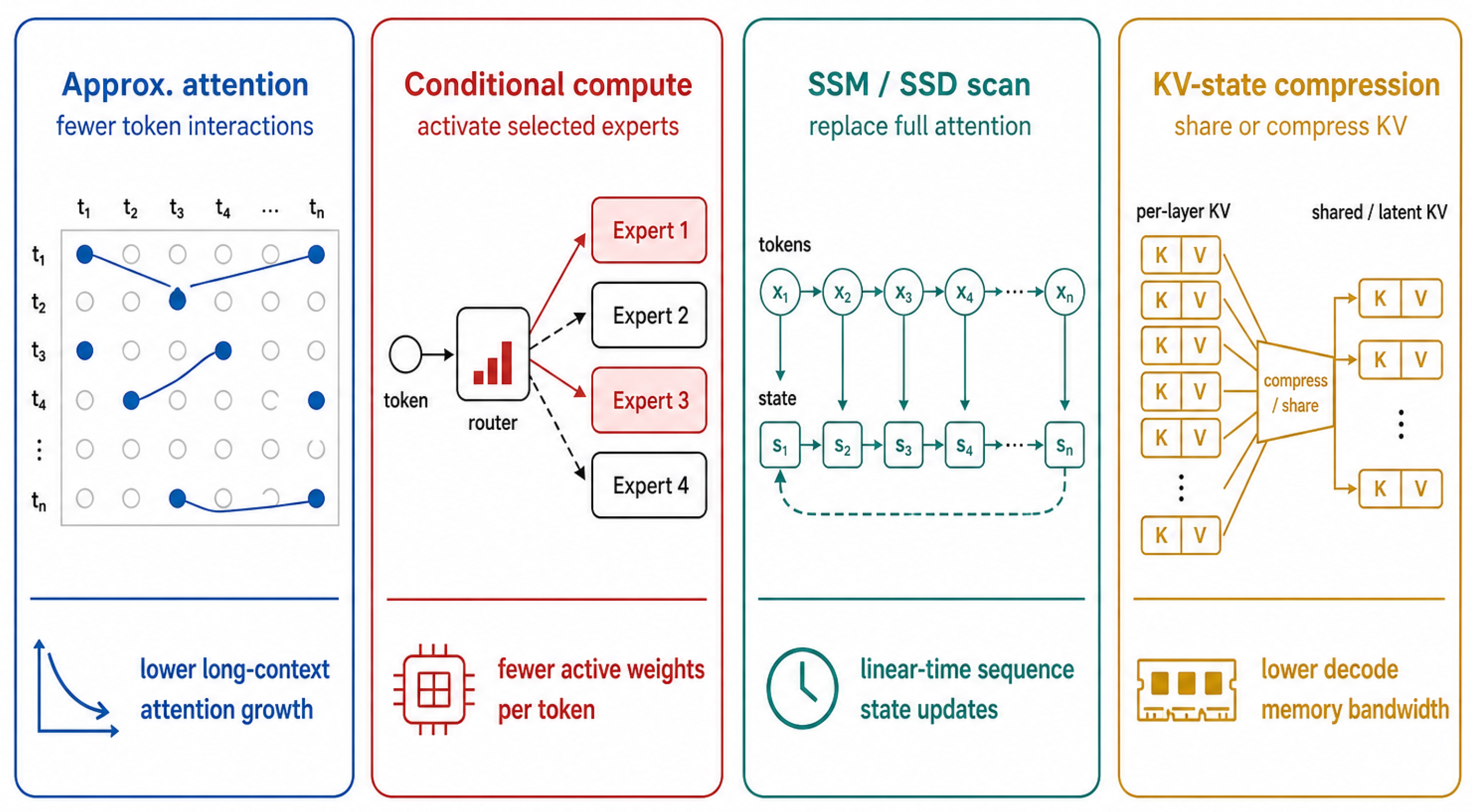
The first algorithmic lever is to change the structure of the computation itself. In transformer models, full self-attention scales quadratically with sequence length, creating a tension between context length and resource usage [4]. Architectural work responds to this bottleneck through mechanisms that reduce token–token interactions, activate only a subset of parameters, replace attention with scan-friendly sequence operators, or compress the attention state used at serving time. Figure 4 summarizes these four mechanisms as complementary ways of changing the workload before runtime and hardware determine realized savings.
Figure 4.
Architecture-level mechanisms for reducing transformer energy. Approximate attention reduces token interactions [35,36,37], conditional computation activates selected experts [8,38], state space model (SSM)/structured state space duality (SSD)-style models replace full attention with scan-friendly state updates [39], and KV-state compression reduces serving-time attention state reads through shared or latent key–value representations [8,40,41,42].
Reducing token interactions. Linear and sparse attention methods such as Linformer [35], Performers [36], and Longformer [37] approximate or restrict the full attention matrix so that long sequences no longer require all-pairs comparison. Their energy value is strongest when the reduced attention pattern maps to efficient kernels and preserves model quality for the target sequence length. Otherwise, the theoretical reduction in attention operations can be offset by irregular memory access, kernel overhead, or lower accuracy that forces the use of a larger model.
Activating fewer parameters. Mixture-of-experts (MoE) models use a router to send each token to a small subset of expert networks rather than activating every parameter [38]. This lowers active FLOPs per token, but also introduces costs that are invisible in comparisons based on parameter count. Recent frontier systems such as DeepSeek-V3 show how fine-grained experts and auxiliary loss-free load balancing are being used to make sparse activation practical at scale [8]. Tokens must still be sorted, dispatched to experts, and gathered back, often across multiple GPUs or nodes. The resulting all-to-all traffic, duplicated expert weights, load imbalance, and idle accelerators can consume a nontrivial share of the theoretical savings, making MoE a routing-and-utilization problem rather than one of reducing active FLOPs.
Replacing full attention. State space models (SSMs) replace the token-by-token attention matrix with a compact recurrent state that is updated as the sequence is scanned. Mamba and Mamba-2 process tokens through structured state space layers, giving linear-time and constant-memory inference for long sequences under the model assumptions [39]. Mamba-2’s Structured State Space Duality (SSD) formulation expresses this computation through structured semi-separable matrices and scan-friendly operations, connecting SSMs to attention while reporting 2–8× speedups over the original Mamba at comparable language modeling quality [39]. The energy gain comes from avoiding the quadratic all-pairs comparison, not from skipping the input sequence (every token is still read).
Compressing attention state. Another architecture-level route keeps exact attention but reduces the size of key–value state that must be stored and read during decoding. Multi-query attention shares one set of keys and values across query heads [40], and grouped-query attention interpolates between multi-head and multi-query attention to reduce KV cache bandwidth while preserving more modeling capacity [41]. DeepSeek-V2 and DeepSeek-V3 push this idea further with multi-head latent attention, which compresses the KV cache into a latent representation and is directly relevant to high-concurrency and long-context serving [8,42]. These variants are best treated as memory system optimizations as much as architectural changes; their benefit grows when KV cache reads, as opposed to arithmetic, dominate generation.
3.2. Model Compression and Reduced-Precision Computing
A key lever keeps the model architecture mostly fixed while reducing the amount or precision of state that must be stored, moved, and multiplied. Compression is attractive because memory movement often dominates transformer energy. This is better understood as a family of methods rather than a single technique. Pruning approaches target sparsity, quantization changes numeric representation, and distillation replaces the served model with a smaller student.
Pruning and sparsity. Pruning removes weights, heads, channels, or layers that contribute little to model performance. The Lottery Ticket Hypothesis shows that dense networks can contain sparse subnetworks capable of matching the original accuracy when trained in isolation [43]. For LLMs, structured approaches such as LLM-Pruner report approximately 20% parameter reduction for LLaMA-7B while retaining 94.97% of average zero-shot classification performance after tuning and without original-corpus retraining data [44]. The deployment issue is that unstructured sparsity creates irregular memory access. H100 accelerates supported structured sparsity patterns, while realized gains depend on kernel and pattern support [7]. Structured pruning is more hardware-friendly, but usually provides lower compression ratios.
Weight and activation quantization. Quantization reduces the bit width used for weights, activations, or both. GPTQ establishes a widely used one-shot route for 3–4 bit weight-only post-training quantization of generative transformers [45], while SmoothQuant shows that smoothing activation outliers can make W8A8 weight-plus-activation quantization practical for LLMs [46]. Activation-aware weight quantization (AWQ) protects a small set of salient weights and enables near-lossless 4-bit weight quantization with reported speedups on supported kernels [47]. These methods mainly reduce memory footprint and bandwidth; their energy benefit is strongest when inference kernels actually use lower-precision data paths rather than dequantizing into higher precision too early.
Sub-2-bit and native low-bit models. Recent work pushes compression beyond conventional 4-bit deployment. QuIP# combines incoherence processing with lattice codebooks for very low-bit LLM quantization [48], and AQLM uses additive multi-codebook quantization to improve the compression–quality trade-off below 3 bits [49]. BitNet b1.58 trains models with ternary weights , replacing many multiplications with additions [50]. Because addition can consume much less energy than multiplication at similar precision [51], native low-bit models are promising for energy efficiency. However, the practical gain depends on whether compilers, kernels, and accelerators expose the intended low-bit arithmetic and memory layout.
Knowledge distillation and model specialization. Distillation trains a smaller student to match the behavior of a larger teacher [52]. Its energy logic differs from pruning and quantization: the served model is a smaller dense model that usually maps well to existing accelerators. DistilBERT, for example, retains most of BERT’s language understanding performance while reducing parameters and improving inference speed [53]. MiniLLM extends objective-level distillation to generation through a reverse-KL training objective [54]. Self-Instruct and Vicuna instead use synthetic instruction or conversation data for model adaptation, and are better treated as related specialization approaches rather than direct distillation methods [55,56]. In both cases, teacher inference, data generation, and task coverage belong within the cost boundary. Distillation or specialization is most compelling when the resulting model will be served many times on a stable workload, so that the one-time transfer cost is amortized over lower lifetime inference energy.
3.3. Training and Adaptation Efficiency
Training-side optimization reduces the energy required to adapt large foundation models to downstream tasks. Full fine-tuning updates every parameter and stores large optimizer states; parameter-efficient fine-tuning (PEFT) instead updates a small set of additional or low-rank parameters. LoRA inserts low-rank matrices into selected weight updates [13], QLoRA combines 4-bit quantization with LoRA to fine-tune 65B-parameter models on a single GPU [14], and DoRA decomposes pretrained weights into magnitude and direction components to improve adaptation capacity without adding inference overhead [57]. These methods mainly reduce training-time memory and optimizer state traffic. The challenge at this stage is that these methods lower the cost of adaptation without necessarily making the base model cheaper to serve, unless the adapter enables a smaller model, lower batch cost, or more specialized deployment.
The evidence boundary is relevant because PEFT papers often report GPU memory, trainable parameter count, or task accuracy, while energy is less frequently measured directly [12,58]. These proxies are still useful because memory footprint constrains batch size and determines whether adaptation can run on fewer or smaller accelerators, but do not necessarily indicate automatic savings. Thus, it is important to distinguish adaptation efficiency from inference efficiency even when both use the same low-bit or low-rank techniques [59].
3.4. Decoding, Multi-Token Generation, and KV Cache Optimization
For deployed generative models, each output token depends on previous tokens; therefore, decoding is often the dominant lifetime cost. Algorithmic serving methods target this serial bottleneck in two ways: they generate or verify multiple candidate tokens per expensive model call, and they reduce the memory burden of the KV cache that grows with context length and concurrency.
Speculative and multi-token decoding. Speculative decoding uses a small draft model to propose several tokens and then verifies those tokens in parallel with the target model, preserving the target distribution under the acceptance rule [60]. A related speculative sampling line reported 2–2.5× decoding speedups on large-model inference without changing sample quality [61]. EAGLE moves the draft process into feature space and reports 2.7–3.5× latency speedup with lossless output quality [62], while Medusa adds multiple decoding heads to the target model so candidate continuations can be generated without a separate draft model [63]. Multi-token prediction (MTP) trains auxiliary heads to predict several future tokens during pretraining, improving sample efficiency and providing a natural source of self-speculative candidates at inference time [64]. DeepSeek-V3 adopts an MTP objective at scale, illustrating that multi-token training has moved from a standalone research idea into frontier model design [8]. Recent block-diffusion draft models such as DFlash further generalize speculative decoding by proposing token blocks in parallel prior to target-model verification [65]. The common energy pathway consists of fewer serial full-model forward passes per accepted output token, but rejected drafts, auxiliary heads, draft model cost, and reduced batching efficiency can offset part of the gain.
KV cache runtime management. The KV cache avoids recomputing past attention states, but grows linearly with sequence length, layer count, hidden size, and the number of concurrent requests; as such, serving runtimes sit at the boundary between model design and scheduling policy. Orca introduces iteration-level scheduling and continuous batching so that requests with different generation lengths can share accelerator time more efficiently [66]. vLLM introduces PagedAttention, which manages KV memory with virtual memory-style paging rather than contiguous pre-allocation, thereby reducing cache waste and improving throughput compared with naive serving [67]. Prefix-aware runtimes target a different source of waste: SGLang’s RadixAttention and Hydragen reuse shared prompt prefixes across structured programs or request batches, reducing redundant prefill work when many requests share system prompts, examples, or retrieved context [68,69]. IO-aware exact attention kernels such as FlashAttention and FlashAttention-2 are complementary because they reduce high-bandwidth memory traffic without changing the mathematical attention result [70,71]. These methods do not change model quality, instead targeting improvements to utilization, memory locality, and cache reuse.
KV cache pruning and quantization. Cache compression reduces the amount of past state retained or the number of bits used to store it, which complements runtime management. H2O and Scissorhands exploit persistent token importance to keep influential cache entries while evicting less useful ones [72,73]. SnapKV compresses long-context prompts by selecting clustered important positions before generation [74], while PyramidKV allocates cache budget across layers according to a pyramidal information pattern [75]. KIVI takes a different route by using tuning-free asymmetric 2-bit quantization for KV cache storage [76]. TurboQuant further frames serving-time KV cache compression as online vector quantization with near-optimal distortion guarantees and reports quality-preserving cache quantization at low bit widths [77]. These methods are directly relevant to energy because KV cache memory controls long-context feasibility, batch size, and attention memory traffic. Aggressive cache reduction still needs quality and kernel checks because attention error, recomputation, or overhead can erase part of the benefit. Figure 5 summarizes these architecture, compression, KV cache, and decoding levers.
Figure 5.
Summary of algorithmic efficiency levers for foundation model workloads. The organizing schematic distills recurring patterns from architecture, compression, KV cache, and speculative decoding studies: architecture methods reshape the computation graph [8,35,38,39]; model state methods reduce stored or updated weights [14,45,50]; KV cache methods page, reuse, prune, or quantize attention history [67,68,72,74,76,77]; and decoding methods verify multiple candidate tokens per target model call [60,63,64,65].
The quantitative evidence for algorithmic efficiency varies because the methods intervene at different points in the model lifecycle. Architecture and decoding changes alter the execution path, compression changes the model state, KV cache methods change serving-time memory pressure, and distillation shifts cost from repeated inference to a one-time transfer process. Table 1 groups results by their optimization target and the deployment condition that determines whether the reported effect can become an energy reduction.
The difficulty at the decoding stage is that algorithmic gains become energy gains only when they remove work from the actual bottleneck. A latency speedup matters most when the workload is serially generation-bound; a reduction in parameters or bit width matters most when kernels and memory traffic preserve the compression benefit, while a reduction in cache memory matters most when long contexts or concurrency make serving memory-bound. This is why proxy metrics can disagree: a method might reduce parameters without reducing runtime energy, or might improve latency while increasing auxiliary computation elsewhere in the serving stack.
The practical implication is that algorithm selection should start from the deployment bottleneck rather than from the largest reported multiplier. Stable high-volume tasks favor distillation or specialization because the transfer cost can be amortized. Long-context serving favors cache and attention-state methods because memory traffic limits batching. Adaptation workloads benefit from PEFT because optimizer-state memory constrains training even if the deployed base model is unchanged. Latency-sensitive generation favors speculative or multi-token methods only when acceptance, batching, and draft overhead preserve the reduction in full-model passes. Thus, the relevant comparison is method plus workload plus runtime plus hardware, not method versus method in isolation.
Table 1.
Quantitative evidence for algorithmic efficiency methods. Rows report the best available numbers from the reviewed literature; entries use different models, hardware, and workloads, and as such are not directly comparable. The table separates the reported effect from the algorithmic target being optimized and that due to the deployment condition needed in order for the target to reduce energy. The “proxy measured” column names the quantity that each cited source actually reports.
3.5. Agentic Workloads and Harness Engineering
Agentic AI changes the unit of analysis from an isolated model call to a multi-step task. An agent may alternate between planning, model inference, tool execution, retrieval, memory updates, verification, and retries before producing a result. In this setting, the energy of a task is not determined by the token count of its final response alone. A useful accounting boundary is
where each term can include both accelerator and host-side energy when those components are inside the study boundary. The decomposition above is intended only as a measurement aid.
The software that controls this execution graph can be viewed as a harness, that is, the prompts, tool interfaces, state and memory policies, routing logic, stopping criteria, verification steps, and retry behavior surrounding the model. Harness engineering extends serving optimization beyond kernel throughput or tokens per second; a harness can reduce energy by selecting a smaller model for routine steps, reusing context, batching independent tool calls, terminating unsuccessful branches early, and preventing repeated work. It can also increase energy through excessive planning turns, redundant context injection, speculative branches, serial tool calls, or retries caused by weak verification. Existing serving mechanisms such as continuous batching, prefix reuse, and KV cache management remain relevant, but their benefit must be evaluated across the complete task trajectory rather than on any single request [66,67,68].
Executable software engineering benchmarks establish the empirical setting in which harness choices can be studied beyond static code generation. SWE-bench evaluates whether an agent resolves repository-level GitHub issues against executable tests [78]. SWE-agent shows that a purpose-built agent–computer interface changes how models inspect repositories, edit files, and run tests [79]. OpenHands broadens this systems view to a platform that combines sandboxed code execution, terminal and browser interaction, multi-agent coordination, and benchmark evaluation [80]. These studies do not measure energy directly, but do identify the action interface, tool surface, runtime, and state management policy as variables that can change both task completion and trajectory length.
Controlled evaluations provide quantitative evidence that the harness is an independent systems variable rather than an incidental implementation detail. On Terminal-Bench 2, GPT-5.2 obtained a task success rate of 62.9% with Codex CLI and 54.0% with Terminus 2, while Claude Opus 4.5 obtained 57.8% with Terminus 2, 52.1% with Claude Code, and 51.9% with OpenHands [81]. These differences are benchmark-specific rather than universal product rankings: even when a nominal model is held fixed, prompts, tool schemas, reasoning settings, runtime limits, and cache accounting can remain harness-dependent. Harness-Bench isolates this execution layer across 106 sandboxed tasks and 5194 trajectories; among its configurable harnesses, aggregate scores range from 52.4 to 76.2, and the highest-scoring configuration also uses fewer tokens than several lower-scoring alternatives [82]. Claw-SWE-Bench likewise reports a 27.4 percentage point range attributable to harness choice under fixed models, which is close to the 29.4-point range attributable to model choice. With the same GLM-5.1 backbone, a minimal direct-diff adapter reaches 19.1% Pass@1, while the full adapter reaches 73.4% [83].
Long-horizon benchmarks also motivate a wider efficiency report than pass rate alone. DeepSWE evaluates 113 original software engineering tasks, reporting output tokens, wall-clock duration, and monetary cost alongside Pass@1 [84]. Because its published configurations use the same mini-swe-agent harness, DeepSWE informs model and reasoning–setting trade-offs within a fixed execution layer rather than providing a causal comparison among harnesses. The Holistic Agent Leaderboard instead evaluates models, scaffolds, and benchmarks jointly over 21,730 rollouts; its analysis shows that increasing reasoning effort does not reliably increase accuracy [85]. Together with the cost-aware evaluation principles in AI Agents That Matter [86], these results support reporting success, tokens, latency, and cost at the model–harness–benchmark configuration level. Most studies that directly isolate harness effects are recent preprints, so their quantitative results should be treated as emerging evidence rather than stable product rankings.
Harness efficiency can also be optimized, but additional components do not automatically result in improvements. Agentic Harness Engineering raised Terminal-Bench 2 Pass@1 from 69.7% to 77.0% over ten iterations and transferred to SWE-bench Verified with 12% fewer tokens than its seed harness; ablations associated this gain primarily with tools, middleware, and long-term memory rather than system prompt changes [87]. In contrast, SWE-Skills-Bench found no improvement in pass rate for 39 of 49 evaluated software engineering skills, an average gain of only 1.2 percentage points, and token overhead as high as 451% for some skills without a gain in success rate [88]. Therefore, the relevant question is not whether a harness contains more planning, memory, skills, or verification but whether each mechanism reduces failed attempts or unnecessary trajectory work for the target workload.
For N attempted tasks, of which complete successfully, a cost-aware evaluation can report
where S is the task success rate, is the mean monetary cost per attempted task, and and are respectively the monetary cost and energy per successful task for . Reporting only cost per attempt can make a cheap but failure-prone harness appear efficient, while reporting only success rate can reward configurations that use excessive calls, context, or retries. Thus, agent evaluations should compare model–harness configurations on a Pareto frontier over task success, cost, energy, and latency rather than collapsing them into a one-dimensional ranking [85,86].
Monetary API cost should not be treated as a direct proxy for energy, as provider prices also reflect caching rules, discounts, hardware utilization, and commercial policy. An energy claim requires either measured power and execution time or a transparent conversion boundary that identifies the included hardware and facility. At minimum, studies should report the exact model and harness versions, reasoning setting, benchmark revision, prompt and tool configuration, token/turn/time budgets, cache accounting, number of model and tool calls, input and output tokens, wall-clock latency, retry rate, and task-level success. Per-call energy can be misleading when a cheaper configuration requires more attempts or produces more downstream tool work; conversely, a larger model may be preferable if it completes the same task reliably in fewer steps. What makes agentic workloads hard to assess is that efficiency is a workload- and harness-level property; thus, improvements at the component level only become environmental savings when they reduce the energy required to complete the same successful task.
3.6. Discussion and Challenges for Algorithmic Efficiency
Three evaluation challenges recur across algorithmic methods. First, proxy metrics are inconsistent; FLOPs, parameter count, perplexity, tokens per second, and peak memory can point in different directions when data movement and utilization are included. Therefore, energy-efficient AI studies should report at least latency, throughput, and memory footprint along with the hardware, batch size, and sequence length used, and, where possible, measured power or energy. A deeper problem is that energy is rarely measured at this layer at all; most algorithmic studies report a speedup, reduction in parameters or bit width, cache savings, or throughput gain rather than the energy drawn by the workload they optimize. For this reason, the proxy-measured column of Table 1 names the quantity that each study actually reports; none of the eleven entries reports measured energy. Direct measurement is the exception, and comes mainly from work designed to measure rather than to optimize, such as the inference energy comparison in Luccioni et al. [33]. Converting a proxy result into an energy value would require assumptions about hardware, batching, and facility conditions that the primary sources do not supply. Closing this gap requires algorithmic studies that report measured power alongside the proxy they already report.
The methods are also not automatically composable. A model can undergo multiple optimizations at once. Typical combinations include distillation, quantization, speculative decoding, and KV cache compression. Even so, the combined effect is not the product of individual speedups. Quantization can change draft-model acceptance, pruning can make kernels less efficient, and cache compression can reduce long-context quality, while continuous batching can shift the trade-off between latency and energy. Thus, the best pipelines will necessarily be workload-specific.
Efficiency must also be tied to the deployment objective. A smaller specialized model is often far more energy-efficient than a general-purpose model for a repeated classification or extraction task, while a larger general model can be justified when one model replaces many task-specific pipelines. Luccioni et al. showed that multipurpose generative models can consume orders of magnitude more inference energy than task-specific systems for equivalent tasks [33]. The system-level question is then not just how to make a given model cheaper, but whether the model is the right size and degree of generality for the workload.
The algorithmic techniques reviewed here reduce the amount, precision, or scheduling rigidity of computation. However, their realized value depends on the physical substrate that executes them. Several algorithmic features place different demands on accelerators and memory systems, for example, irregular sparsity, low-bit arithmetic, long-context attention state, and continuous batching. Next, Section 4 turns from how to reduce computational demand to ways of reducing the energy cost of executing that demand.
4. Hardware Efficiency
Hardware efficiency determines whether the workload reductions discussed in Section 3 become physical energy savings. Even when a model uses fewer FLOPs, lower precision, or a smaller KV cache, it still has to move its entire state through a memory hierarchy, including weights, activations, optimizer states, and attention. The relevant metric at this layer is useful work delivered per joule after accounting for memory traffic, communication, utilization, and software support.
4.1. Hardware Constraints on Energy Efficiency
The energy hierarchy of modern hardware explains why AI efficiency is often a data movement problem. Horowitz’s 45-nm reference table shows that off-chip dynamic random-access memory (DRAM) access is orders of magnitude more expensive than small arithmetic operations and substantially more expensive than local static random-access memory (SRAM) access [51]. Although the absolute values are technology-specific, this access energy hierarchy remains directionally useful. In profiled Google consumer workloads, data movement accounted for 62.7% of total system energy on average [89]. Transformer inference inherits the same bottleneck: every generated token requires weight reads, activation movement, and repeated access to the KV cache state.
Hardware claims should be interpreted relative to the workload that actually runs on the device. Peak TOPS/W, tensor core throughput, or narrow-precision support are valuable only when the model, compiler, kernels, and runtime keep the device fed with useful work. If an algorithm produces irregular sparsity, low arithmetic intensity, poor batching, or excessive all-to-all communication, the accelerator can spend energy moving and waiting rather than computing. Thus, hardware efficiency is best evaluated as a workload-specific mapping problem.
4.2. Accelerator Data Paths and Workload Fit
AI accelerators have evolved by specializing the data path used for matrix and tensor operations. Central processing units (CPUs) remain flexible, but are poorly matched to the parallel dense linear algebra that dominates deep learning. GPUs improve the match through massive parallelism, high-bandwidth memory, and tensor cores. Successive NVIDIA generations have added support oriented towards BF16, TF32, FP8, and FP4 [7,16,90]. These advances matter in practice, but are not energy guarantees; their realized benefit depends on sequence length, batch size, precision format, sparsity pattern, and whether kernels avoid unnecessary data conversion.
Application-specific integrated circuit (ASIC)-style accelerators narrow the design target further. Tensor processing units (TPUs) and Trainium use custom tensor data paths, interconnects, and low-precision modes for large-scale training and inference [91,92]. Wafer-scale and dataflow systems such as Cerebras WSE-3 and Graphcore Bow IPU reduce off-chip or off-package communication by changing the physical organization of compute and memory [93,94]. Edge and mobile neural processing units (NPUs), including Apple’s Neural Engine, emphasize local execution and fixed-function throughput for selected workloads [95]. In this review, these platforms are used as examples of design levers, with each exposing a different trade-off among programmability, utilization, memory locality, and deployment context.
4.3. Memory Systems and Data Movement
The most consistent hardware theme is to shorten the path between data and computation. High-bandwidth memory (HBM) stacks DRAM close to the processor, thereby raising bandwidth while reducing energy per bit relative to conventional off-package memory. Reported HBM3/HBM4 trends emphasize higher bandwidth per watt and lower energy per transferred bit [96]. Advanced packaging, interposers, hybrid bonding, and 3D integration pursue the same objective by reducing interconnect length and communication energy. Carbon nanotube 3D integration is a more experimental version of this idea, demonstrating vertically stacked logic, memory, sensing, and dense inter-layer connections for energy-efficient nanosystems [97].
Inter-chip communication is another major cost. Electrical links consume energy even when computation is efficient, which matters for distributed training, MoE routing, tensor parallelism, and large inference clusters. Optical interconnects and photonic devices reduce the energy of long-distance data movement and can also implement matrix operations optically [98]. Taichi, for example, reports 160 TOPS/W in a photonic chiplet demonstration [99]. While such results show the potential of light-based data movement and computation, the full system still has to handle nonlinear layers, normalization, memory access, digital control, and integration with conventional accelerators. Figure 6 groups the hardware routes that shorten, localize, or avoid data movement.
Figure 6.
Hardware efficiency as data movement reduction. HBM and advanced packaging shorten memory paths [96,97]. On-chip SRAM architectures such as NorthPole [100], processing-in-memory (PIM) accelerators such as PIM-GPT [101], and photonic systems such as Taichi [99] target efficiency by shortening, localizing, or avoiding the movement of weights and activations.
4.4. Near-Memory, In-Memory, and Event-Driven Designs
A more radical strategy is to place memory and compute in the same physical fabric. IBM’s NorthPole co-locates all model memory on chip, and reports a 25× higher energy metric (frames per second per watt) than comparable GPUs on ResNet-50 inference [100]. The benefit comes from avoiding off-chip movement when the model partition and workload fit the available on-chip memory. Figure 7 redraws the study’s ResNet-50 iso-energy comparison as an example of workload-specific hardware evidence.
Figure 7.
Panel (a) shows a reconstruction of the ResNet-50 iso-energy comparison reported by Modha et al. Each point uses the throughput from Table 1 of that paper on the vertical axis and energy metric divided by throughput on the horizontal axis, so the dashed contours denote constant frames per joule; panel (b) enlarges the boxed region. In Table 1 of Modha et al. [100], energy is a reported value when available and is otherwise calculated as throughput divided by thermal design power.
Processing-in-memory (PIM) moves selected operations into or near memory arrays rather than repeatedly transferring data to separate compute units. For autoregressive transformers, this is directly relevant to weight streaming, attention state access, and KV cache movement. In the reported PIM-GPT evaluation, models up to 1.4B parameters achieved 41–137× speedup and 123–383× gains in energy efficiency over GPU baselines under the evaluated model sizes, baselines, and mapping assumptions [101]. The boundary condition is that PIM gains are strongest for operations that map cleanly to memory array computation; nonlinear layers, control flow, inter-array coordination, and full model integration can reduce the realized advantage.
Neuromorphic hardware pursues efficiency through event sparsity rather than dense matrix throughput. Loihi-class systems integrate memory and computation in a spiking event-driven fabric, and Intel’s Hala Point reports up to 15 TOPS/W for selected sparse workloads [102,103]. These devices are promising for sparse, temporal, or event-based workloads, but most foundation model pipelines are not naturally expressed as spiking computations; their energy relevance depends on software maturity and workload reformulation as much as on device-level efficiency.
4.5. Reduced Precision as a Hardware Feature
Low-bit algorithms save energy only when hardware exposes the corresponding data paths. Modern accelerators increasingly support BF16, TF32, FP8, INT8, and emerging 4-bit or FP4-style formats [7,90,91]. This matters because reduced precision can lower both arithmetic energy and memory bandwidth energy. Mixed-precision training, for example, can improve throughput and reduce memory traffic compared with FP32 training when kernels and loss scaling preserve accuracy [104].
A second difficulty is that algorithmic bit width and hardware bit width are not automatically the same. A 4-bit or 2-bit model typically still requires dequantization, scale factor handling, packing overhead, or fallback kernels. Weight-only quantization mainly reduces memory footprint and bandwidth, whereas weight-plus-activation quantization can expose more low-precision arithmetic. Native low-bit models such as BitNet-style ternary networks require even tighter compiler and hardware support. Reduced precision is a cross-layer optimization: the algorithm selects a representation, while hardware and software determine whether that representation reduces measured energy.
4.6. Software–Hardware Co-Design
Hardware capability becomes useful only when the software stack exposes it. Several software mechanisms change utilization and energy per token: compiler optimizations, kernel fusion, memory planning, collective communication algorithms, power capping, and dynamic batching. These software mechanisms are as important as the silicon itself. Gradient checkpointing demonstrates this trade-off: it reduces activation memory by recomputing intermediate values, which can enable a smaller memory footprint or larger batch but also adds arithmetic work. Similarly, sparsity and low-bit arithmetic require kernels that avoid spending the saved energy on indexing, packing, or dequantization overhead.
Large-scale training and serving systems make co-design even more important. Llama 3 training used a large H100 cluster and custom network fabric to reduce communication bottlenecks [19]. TPU v5e/v6 systems combine accelerator design, optical circuit switching, and scheduling to improve energy per training step [91]. These examples should be seen as evidence that accelerator efficiency is a system property. The chip is only one component, and the compiler, runtime, interconnect, parallelization strategy, and cluster scheduler together determine how much of the chip-level capability is realized.
4.7. Quantum and Hybrid Quantum–Classical Accelerators
Quantum computing is sometimes discussed as a post-CMOS route to efficient computation, but is not yet a direct replacement for AI accelerators. Quantum processors exploit superposition, entanglement, and interference for selected problem classes, and near-term AI use is most plausibly hybrid. Parameterized quantum circuits can be optimized by classical routines, as in variational quantum algorithms [105]. Current noisy intermediate-scale quantum devices remain limited by qubit count, noise, circuit depth, and lack of large-scale fault tolerance [106].
Energy accounting for quantum acceleration must include the full control system. Superconducting platforms require cryogenic cooling, microwave control, heat load management, state preparation, measurement, and classical postprocessing. Work on energy-efficient quantum control has shown that reusing and correcting drive pulses can reduce average gate energy without increasing average gate error [107], while measurement studies have identified scaling control signals as a central barrier [108]. Quantum and hybrid quantum–classical accelerators are treated here as long-horizon research directions. Their relevance to energy-efficient AI depends on useful workloads that can offset the overhead related to state preparation, error handling, cooling, and classical control.
4.8. Hardware Platform Comparison
Table 2 separates three kinds of hardware evidence that are often conflated: device-level energy constants, workload-level efficiency comparisons, and peak throughput-per-watt demonstrations. This separation is important because per-access energy numbers, end-to-end inference comparisons, and laboratory TOPS/W claims all describe different levels of system behavior. Therefore, the table identifies the hardware mechanism, what the reported number measures, and the evaluation setting in which it was obtained. In this way, each entry pairs a proposed approach with the gain claimed for it and the conditions that limit that claim.
Table 2.
Quantitative evidence for hardware approaches. Rows report the best-available numbers from the reviewed literature; entries use different models, hardware, and workloads, meaning that they are not directly comparable. The table separates the hardware mechanism from what the reported number measures and the evaluation setting in which the number was obtained.
The above comparison reinforces the simple rule that hardware efficiency is meaningful only within a workload and measurement boundary. The first two rows explain why memory locality is a physical energy lever; the middle rows show how near-memory or on-chip memory designs can improve specific inference workloads; and the final rows report specialized throughput-per-watt demonstrations. A platform can be excellent for dense batched tensor operations, long-context memory traffic, sparse event streams, or optical linear algebra, yet lose its advantage when software, interconnect, control logic, or cooling overheads move the workload outside the measured boundary.
4.9. Discussion and Challenges for Hardware Efficiency
Comparing results across hardware studies is limited by benchmark boundaries, software maturity, and deployment specialization. Some reports measure chip energy, while others report board or server energy and still others include cluster communication. Cooling, power delivery, and utilization are often outside the scope of hardware papers even though they affect wall-plug energy. GPUs benefit from a mature software stack that includes compilers, kernels, and scheduling tools, while PIM, photonic, and neuromorphic systems often require workload-specific mapping. Specialization creates a deployment trade-off in which a narrow accelerator can be extremely efficient in its sweet spot, but often requires additional hardware, data movement, or scheduling complexity.
These limits clarify how hardware innovation should be evaluated. The strongest evidence connects a device mechanism to an end-to-end workload, from model and precision configuration to the measured energy boundary. Hardware determines the energy cost of useful computation; however, accelerators do not operate in isolation: their environmental impact also depends on facility power overhead, cooling demand, water consumption, workload placement, and grid carbon intensity. Therefore, the next section moves from accelerator execution to the data center and grid infrastructure in which AI hardware is deployed.
5. Data Center and Infrastructure Efficiency
Algorithms and hardware operate within data center infrastructure, where facility-level overhead and environmental intensity add to IT load. Global data center electricity consumption reached 415 TWh in 2024 (1.5% of world demand) and is projected to reach 945 TWh by 2030 [1]. In the United States alone, consumption grew from about 60 TWh in 2014 to 176 TWh in 2023, with projections of 325–580 TWh by 2028 [2]. For notable AI systems, the Stanford HAI 2025 AI Index reports rapid scaling indicators showing that training compute doubles every five months, datasets double every eight months, and power use doubles annually [109]. These data center and AI system trends place pressure on cooling, power distribution, energy sourcing, and workload scheduling. Figure 8 frames that coordination as an operational control loop: workload flexibility and grid signals determine which jobs can be shifted, paused, checkpointed, power capped, or routed while still protecting latency-critical services.
Figure 8.
Grid-interactive AI data center control loop. Infrastructure efficiency depends on the interaction among workload urgency, grid carbon and reliability signals, local thermal and water constraints, and facility-level controls such as power capping, checkpointing, routing, and scheduling.
5.1. Advanced Cooling Technologies
Cooling and auxiliary infrastructure vary widely by facility. The IEA reports cooling shares from below 10% in efficient cloud data centers to over 30% in less-efficient enterprise facilities, and the rise of high-power accelerated servers increases heat density pressure [1]. Traditional air-based computer room air conditioner/computer room air handler (CRAC/CRAH) systems can struggle as rack and server power density rise [1,110]. Thus, liquid cooling has emerged as the primary alternative for high-density deployments.
Water and specialized coolants can provide much higher heat transfer capacity than air; Haghshenas et al. reported that immersion cooling achieved almost six times higher power density and approximately 50% lower energy consumption compared with air cooling under their evaluated settings [110]. Direct-to-chip (D2C) systems such as RackCDU route coolant directly to processor heat sinks. Asetek reported that RackCDU deployments can reduce cooling energy consumption, and a California Energy Commission-funded project installed RackCDU in approximately 90 racks across two large California supercomputing data centers to evaluate energy and cost savings under operational conditions [111,112]. Immersion cooling goes further, submerging entire servers in dielectric fluid. Two implementations exist: single-phase immersion, where servers are placed directly into the coolant with no state change, and two-phase immersion, where a specialized dielectric fluid boils on contact with hot components and is recondensed through a heat exchanger. The relative economics, maintenance requirements, and cooling performance of single-phase, two-phase, and D2C systems are all dependent on facility design and operating conditions [110].
Software-based optimization can complement hardware cooling. In a 2014 provider-reported Google case, Gao showed that neural network models can predict data center PUE within approximately 0.4% error from operational sensor data [113]. Cloud providers, vendors, or facility operators report many infrastructure results, including PUE, cooling control, and facility retrofit numbers. The infrastructure evidence is constrained at the source, since production data centers are difficult for outside researchers to instrument; such sources represent operational case studies rather than fully peer-reviewed benchmarks. For this reason, infrastructure results are treated below as evidence-bound case studies rather than directly comparable benchmarks.
5.2. Power Distribution and Overhead
In addition to cooling, power distribution losses between the grid and chip also contribute to facility overhead. Each AC–DC or DC–AC conversion results in energy loss; together with cooling and other auxiliary systems, power conversion and distribution losses also form part of the non-IT overhead captured by PUE [1,31].
The industry-standard metric for quantifying this overhead, power usage effectiveness (PUE), is defined as total facility energy divided by IT equipment energy. The Uptime Institute reports that average global PUE has remained largely flat in recent years [114], whereas Google reports a PUE of 1.09 across its large-scale data centers [115]. These values are not directly interchangeable because facility design, climate, utilization, and accounting boundaries differ.
Because PUE multiplies the IT load, modest changes in facility overhead can produce large absolute energy differences at scale; nevertheless, cross-site comparisons require matched workload and accounting boundaries.
One notable development is the adoption of 48V motherboards. In 2016, Google announced 48V-direct-to-CPU motherboards, reporting that the improved system power usage effectiveness (SPUE) with 48V had saved millions of dollars and kilowatt-hours compared with 12V solutions [116].
Water use adds a second infrastructure constraint beyond electricity demand. Water usage effectiveness (WUE), defined as annual site water usage divided by IT equipment energy consumption (L/kWh), complements PUE by capturing the water footprint of cooling systems. Where evaporative cooling towers are used, cooling can add substantial site water demand [28]. Jegham et al. [28] estimated that annual water footprint of GPT-4o ranges from approximately 1.3 to 1.6 million kiloliters under their deployment and cooling assumptions. Their modeled scenarios also showed that identical models can exhibit nearly 6× differences in separately reported water consumption and carbon emissions depending on the hosting data center [28] (see Figure 9), showing that infrastructure choices and not just model design shape the estimated environmental impact. As rack densities climb and water-scarce regions host more data center capacity, WUE reporting and recirculating cooling designs become useful complements to energy optimization.
Figure 9.
Qualitative boundary map for infrastructure-dependent per-query water and carbon outcomes. PUE, WUE, cooling technology, grid mix, location, time, and routing policy can change the resource intensity of an identical model request. Water and carbon should be reported separately in their native units under matched system boundaries; the figure does not define or imply a composite footprint [28].
5.3. Renewable Energy Integration
In parallel with reducing facility overhead, lowering the carbon intensity of supplied electricity can reduce the carbon footprint of AI workloads. In 2025, natural gas and coal supplied about 58% of U.S. utility-scale electricity generation, while renewables supplied about 24% [117]. Major technology companies have announced renewable or carbon-free energy procurement goals, although the accounting mechanisms and hourly matching levels differ across firms [118].
Intermittency remains a major obstacle. Data centers require consistent and reliable power, while solar and wind energy are subject to weather variability. Battery energy storage systems (BESS) using lithium-ion batteries can store energy during peak production; in the cited EIA sample, installations classified as long-duration averaged 4.2 h of discharge rather than multi-day resilience [119]. In the cited McKinsey analysis, firming wind and solar with lithium-ion storage typically exceeds $200 per MWh, while longer-duration hydrogen or green ammonia storage could reduce the modeled cost below $100 per MWh [120].
These limitations have renewed interest in nuclear energy as a source of firm low-carbon power that can complement renewable-heavy systems under suitable operational and regulatory conditions [121]. Recent procurement plans span both existing plants and proposed small modular reactors: Microsoft contracted for approximately 835 MW from a planned restart of Three Mile Island Unit 1, Google agreed to purchase up to 500 MW from Kairos Power, and Amazon announced investments targeting more than 5 GW of prospective capacity together with an agreement supplied by the existing Susquehanna plant [122,123,124,125]. These commitments indicate commercial interest rather than deployed evidence; construction cost and regulatory timelines make nuclear power a possible long-term supply option rather than a near-term efficiency intervention [122,123,124,125].
5.4. Grid-Interactive Data Centers and Demand Response
While renewable integration addresses the supply side of the problem, AI data centers can also become more flexible on the demand side. Grid-interactive data centers treat AI workloads as controllable electrical demand, modulating load in response to grid signals, electricity prices, renewable availability, or emergency reliability events. Consumption is not treated as fixed. The U.S. Department of Energy identifies this temporal and spatial flexibility as a priority for powering AI infrastructure, noting that data centers can support the grid by shifting flexible computation across time or location and by participating in demand-response programs [118].
Because not all computations have the same latency requirements, certain AI workloads are more suitable for this approach. While interactive inference must satisfy tight response-time service-level agreements (SLAs), many training jobs, hyperparameter sweeps, offline embedding generation, model evaluation runs, and batch inference tasks can tolerate minutes to hours of delay. These workloads can be paused, slowed, checkpointed, geographically shifted, or scheduled during periods when renewable generation is abundant and grid carbon intensity is lower. Conversely, during grid stress events, facilities can reduce non-urgent GPU utilization, defer batch jobs, or temporarily lower power caps while preserving high-priority real-time services. Demand response connects renewable energy integration with carbon-aware scheduling.
A 2025 Phoenix field demonstration on a 256-GPU cluster in a commercial cloud data center reduced cluster power by 25% for three hours during a summer peak event using software-only controls while maintaining performance for high-priority workloads [126]. Such results suggest that cluster-level flexibility need not require shutting down an entire facility, as it can instead be implemented through workload-aware orchestration, power capping, checkpointing, and prioritization policies. The remaining problem is operational; schedulers must jointly respect grid signals, thermal constraints, hardware heterogeneity, job deadlines, and user-facing SLAs. In deployment, measured workload flexibility informs both infrastructure planning and model serving design.
5.5. Workload Scheduling
In addition to cooling, power delivery, and energy sourcing, workload scheduling offers additional savings by deciding when and where to run each job. By the definition of PUE, the IT share of facility energy is [31], so scheduling directly controls the workload component of operational power draw. Scheduling can be considered along three dimensions: (1) job scheduling, which determines machine or cluster assignment; (2) task scheduling, which considers how to partition jobs for parallel or sequential execution; and (3) resource scheduling, which maximizes utilization across components.
Google’s Borg cluster manager runs hundreds of thousands of jobs from many thousands of applications across clusters with up to tens of thousands of machines. By co-scheduling jobs in batched workloads on shared machines rather than segregating them on individual clusters, it avoids 20–30% additional machine resource overhead [127]. Alibaba’s “tidal scaling” approach dynamically reclaims underutilized memory from online service jobs during off-peak traffic periods to improve both efficiency and cost [128]. Neither system was designed with energy as its primary objective, yet the outcome (fewer idle machines and higher utilization) can reduce power draw and cooling load when idle capacity is powered down or avoided, making scheduling a de facto energy lever even when it is not framed as one.
Thermal-aware scheduling (TAS) algorithms distribute workloads with temperature in mind, shifting load away from zones with elevated temperatures that would require additional cooling energy. In the evaluated GPU scheduling scenario, ThermalAwareGpu achieved up to 12.79% computing cost savings compared with baseline algorithms, though the study did not establish the same percentage as a direct energy reduction [129]. TAS can also prevent temperature spikes that cause hardware degradation and potential downtime [130]. As rack power density rises, thermal-aware scheduling becomes more relevant to both reliability and cooling energy.
Figure 10 provides a request-level serving energy example in which prompt length changes modeled load. While this is not a scheduling result, it illustrates why workload characteristics must be reported prior to scheduling comparisons.
Figure 10.
Modeled per-request energy for short, medium, and long GPT-4o prompts and a per-search Google baseline, redrawn from Jegham et al. [28]. All bars use a request-level functional unit, but actual energy still depends on prompt length, model configuration, batching, serving hardware, and data center conditions.
An emerging complement to thermal-aware scheduling is carbon-aware scheduling, which shifts workloads in both space and time based on the real-time carbon intensity of the electricity grid. Lechowicz et al. proposed PCAPS for data processing jobs with task precedence constraints [131]. In simulation (averaged over six grid traces), a moderately carbon-aware setting reduced emissions by 39.7% relative to first-in, first-out (FIFO) scheduling. A prototype with 100 Spark executors on Kubernetes also reduced emissions by up to 32.9% relative to default Spark/Kubernetes scheduling on the workloads and carbon traces in that study. On a single motivating directed acyclic graph (DAG), C-OPT reduced emissions by 51.2% versus FIFO but increased makespan by 28.5%. On that same DAG, PCAPS reduced emissions by 23.1% and finished 7% earlier than FIFO.
5.6. Summary of Infrastructure and Cross-Layer Evidence
Table 3 groups infrastructure evidence by what changes in the system. The training energy rows report workload electricity, while the carbon and water rows translate that electricity through grid or cooling assumptions. The facility rows report overhead ratios or power delivery improvements, and the scheduling rows change when or where computation runs. In this way, the table emphasizes the infrastructure lever, the system quantity that changes, and the provenance of the number (operator disclosure, independent estimation, modeled scenario, simulation, or operational case study). Read across the rows, the reported values record the progress made by infrastructure work, while the provenance entries record where the evidence for such progress is still thin.
Table 3.
Quantitative evidence for infrastructure techniques, workload accounting, and cross-layer estimation tools. Rows report the best available numbers from the reviewed literature; entries use different models, hardware, workloads, and facility conditions, meaning that they are not directly comparable. The table separates each evidence item from what it changes in the system as well as from the provenance of the reported value.
The techniques in Table 3 operate at different points in the infrastructure stack. The training energy and per-query rows measure the workload itself; the PUE, cooling, and 48 V rows reduce the facility overhead attached to that workload; carbon-aware scheduling changes the grid intensity of the electricity consumed; and water footprint depends on both cooling technology and regional conditions. The evidence sources are equally mixed, ranging from operator disclosures and model cards to independent estimates, simulations, and provider case studies. For this reason, infrastructure evidence is strongest when a paper states both the physical resource being reduced and the boundary over which the reduction is counted.
5.7. Discussion and Deployment Barriers
Because facility overhead applies to every workload, infrastructure optimization can produce large absolute savings. The attainable reduction depends on site design, climate, utilization, and retrofit constraints rather than on transferring a hyperscale PUE value directly to another facility. However, realizing these savings at scale faces economic and technical barriers as well as organizational constraints. Immersion cooling delivers clear thermal advantages, but requires purpose-built facilities or major retrofits; for many co-location providers operating legacy buildings, the capital cost is difficult to justify. Renewable intermittency creates a different constraint, since lithium-ion storage durations remain limited. The cited Google and Kairos deployments target operation around 2030 [119,123]. Because AI demand is growing before these long-term supply options are fully available, near-term operation will depend on a mix of efficiency, procurement, storage, and workload flexibility.
Infrastructure benefits are also distributed unevenly across the industry. Hyperscale operators can report very low PUE because they design custom facilities, control more of the stack, and operate at a scale that justifies dedicated engineering investment. A mid-size enterprise renting space in an older co-location facility has less control over cooling, power delivery, and energy sourcing. Renewable energy availability also varies by geography; a data center in a grid with plentiful hydro or geothermal power will have a different carbon profile from one located in a region where the grid relies heavily on fossil fuels. These differences mean that identical models deployed in different facilities can have substantially different carbon and water footprints [28].
Infrastructure also changes the meaning of model- and hardware-level efficiency claims. A model used for offline embedding generation can be scheduled during off-peak hours when renewable energy is abundant, cooling demand is lower, and electricity is cheaper. A real-time conversational model cannot rely on the same flexibility, and must run when demand arrives regardless of grid carbon intensity or thermal conditions. The same architecture can impose different infrastructure requirements depending on its serving pattern. Carbon- and thermal-aware scheduling algorithms show promise individually, but integrating them with production cluster managers that must simultaneously respect latency SLAs, hardware heterogeneity, and energy constraints remains uncommon in public evidence.
The infrastructure layer shows why energy-efficient AI should not be evaluated solely at the model or accelerator level. A model’s footprint depends on workload flexibility, facility design, cooling technology, water use, and grid conditions. These dependencies motivate the questions in Section 6 around standardized measurements, cross-layer benchmarks, reporting practices, and deployment strategies that connect design intent to operational outcomes.
6. Challenges and Future Directions
The evidence surveyed in Section 3, Section 4 and Section 5 remains uneven across workloads and deployment settings. This section asks which aspects would lower energy use rather than what would make a component faster, and works from the evidence collected in the three summary tables. Open questions concern measurement, cross-layer evaluation, lifecycle accounting, and the translation of component-level gains into deployed energy reductions.
6.1. Measurement, Metrics, and Transparency
Energy measurement across AI systems remains inconsistent and difficult to compare. Because deployed models are queried repeatedly, inference can represent a large share of lifecycle energy [10,11]; however, it receives only a fraction of the measurement attention devoted to training. Jegham et al. [28] estimated that per-query energy can vary by more than 65× across models under long-prompt settings, but few studies have systematically profiled inference under realistic serving conditions, with most reporting only accuracy, latency, or throughput.
Thus, a model that achieves 1% higher accuracy but consumes 10× more energy per query will appear superior under accuracy-only evaluation, but is difficult to justify at deployment scale [33]. Without including energy in the evaluation loop, the research community must rely on limited evidence when comparing models on a dimension that increasingly shapes deployed cost.
The absence of agreed-upon measurement protocols compounds the above problem. While training energy is occasionally reported, methodologies vary so widely (different system boundaries, hardware configurations, and attribution methods) that cross-study comparison is unreliable [12]. Estimation tools have begun to fill this gap: LLMCarbon predicts training emissions within 8.2% of measured values [32], and Green Algorithms quantifies the carbon footprint of arbitrary computational processes [132]. The literature on Green AI argues for reporting efficiency alongside accuracy [30], yet adoption remains limited.
A practical next step would be for papers that report accuracy on standard benchmarks to also report energy consumption measured with a specified tool on a reference hardware configuration. Venues such as NeurIPS and ICML have experimented with reproducibility checklists; extending these to include energy would add some overhead, but would also make comparisons more transparent.
Table 1, Table 2 and Table 3 summarize the quantitative evidence reviewed in this paper, distributed across the corresponding system layers. The tables are not benchmark rankings; their purpose is to identify what each study actually measured and where translation to deployed energy remains uncertain. The algorithmic table is organized around optimization targets, as many results are proxies such as latency, bit width, perplexity, model size, or KV cache memory. The hardware table is organized around mechanisms and boundaries because access-level physics, workload-level efficiency ratios, and specialized throughput-per-watt demonstrations are not interchangeable. Finally, the infrastructure table is organized around affected resources and evidence basis since electricity, carbon, water, PUE, and scheduling outcomes depend strongly on whether the value is operator-disclosed, modeled, estimated, or simulated. Across all three tables, the recurring evidence gap consists of the absence of shared boundaries for converting those numbers into impact on wall-plug energy, carbon, or water usage.
6.2. Cross-Layer Co-Design and Evaluation
Even with better measurement, an efficient component does not automatically create an efficient system. Cross-layer co-design means that model designers, hardware architects, runtime developers, and data center operators optimize against a shared energy objective instead of optimizing their own layer independently. This issue can be seen in a simple example. A pruning method may remove 80% of a model’s FLOPs, but if the remaining weights form irregular sparse tensors that the target GPU cannot execute efficiently, then the measured energy reduction can be small. The remaining benefit can be reduced even further by low server utilization, cooling overhead, or operation in a carbon-intensive grid region [24]. Suboptimal scheduling, underutilized hardware, and inefficient runtime configurations each contribute to waste that algorithm-level metrics will never capture [24].
The practical goal is to ensure that each layer exposes information that the other layers can use. At the hardware–software boundary, compiler-level operator fusion, memory-aware scheduling, and precision adaptive kernels can reduce redundant memory accesses. Hardware could expose energy-relevant controls such as dynamic voltage–frequency scaling, precision selection, and memory hierarchy hints to higher-level frameworks, thereby replacing one-size-fits-all defaults with application-aware energy management. At the broader system level, evaluation can trace energy across IT equipment and data center infrastructure, allowing researchers to identify where measured gains occur [133]. Shared benchmarks and cross-community venues that bring together ML researchers, chip architects, and facility engineers would make this translation easier to evaluate.
A useful primary-study benchmark would run a fixed inference workload under a small factorial design rather than inferring a combined gain from component-level multipliers. One design could compare full precision with 4-bit quantization, a general-purpose GPU with an accelerator that has native low-precision support, and two explicitly defined facility overhead profiles. Reporting wall-plug energy, latency, throughput, and facility overhead for each configuration would show whether algorithmic and hardware gains survive real batching, memory traffic, and cooling overhead.
6.3. Rebound Effects and Lifecycle Impacts
Technical efficiency gains are important, but because of the Jevons paradox, they are not sufficient. As AI becomes cheaper per query, demand may expand enough to offset per-unit improvements; whether aggregate consumption grows then depends on the resulting demand response. The broader ICT literature has documented this pattern, with digital efficiency gains frequently offset by scale, new services, and indirect demand effects [27]. Data center histories show that efficiency improvements and demand growth must be evaluated together [133]. The rapid growth of training compute makes it necessary to evaluate demand alongside efficiency improvements [3]. Per-unit efficiency targets without transparent demand accounting can coexist with rising aggregate consumption.
Reporting and disclosure rules are relevant here mainly because they can change what evidence is available for comparison. Germany’s EnEfG requires covered data center operators to report energy use, renewable electricity share, and facility efficiency indicators [134]. Such requirements do not solve the technical problem of efficient AI, but can make energy use, facility overhead, and carbon intensity more visible. Carbon-aware schedulers need this information when certain jobs can be delayed or be placed elsewhere [131].
The accounting boundary itself also remains narrow. Current evaluations focus mainly on operational energy, but semiconductor fabrication and frequent hardware replacement can amplify embodied lifecycle emissions [135]. Gupta et al.’s Chasing Carbon study shows that embodied emissions can represent a large share of computing system footprints and that advanced-node chip manufacturing affects efficiency claims [135]. Public device-specific embodied carbon data for accelerators such as H100 remain sparse, which makes exact per-GPU manufacturing kWh or kgCO2e difficult to compare across vendors. Water consumption is similarly underreported: Jegham et al. [28] estimated GPT-4o’s annual water footprint at 1.3 to 1.6 million kiloliters under deployment scenarios that vary by cooling technology. A more complete picture of AI’s environmental cost would go beyond the electricity consumed during training or inference to cover manufacturing, transportation, operational water and energy usage, and end-of-life disposal.
6.4. Emerging Technologies and Deployment Frontiers
The neuromorphic, photonic, and processing-in-memory architectures discussed in Section 4 have reported high efficiency in controlled settings. However, the path from laboratory demonstration to production deployment remains long and uncertain for each technology.
Loihi-class neuromorphic processors target sparse event-driven spiking workloads, but their programming tools and training methods remain less mature than those used for dense transformer models [102,136]. NorthPole is a memory-centric dataflow architecture for conventional neural network inference, so its deployment constraints concern model mapping, on-chip capacity, and software support rather than a spiking programming model [100]. Taichi reports high efficiency for a shallow distributed hybrid photonic architecture, while translation to architectures with different layer and memory profiles remains unverified [99]. PIM-GPT uses a companion ASIC for nonlinear functions and communication and evaluates models up to 1.4B parameters through circuit synthesis and cycle-accurate simulation [101].
A complementary frontier involves workload placement at the edge. MCUNet shows that edge deployment can enable analytics near the sensor under tight latency, energy, memory, and storage constraints [137]. This approach can also shift energy consumption from shared data centers to consumer devices, duplicate hardware, and reduce utilization if workloads are too intermittent.
Near-term impact will likely come from matching each technology to workloads where its reported energy advantage survives software, interconnect, cooling, and accounting overhead. Emerging technologies are best discussed as workload-specific options rather than as general replacements for existing accelerator platforms.
Taken together, these issues point to the same need: reported efficiency gains are most useful when connected to measured deployment outcomes. Without standardized reporting, cross-layer benchmarks, lifecycle accounting, and attention to rebound effects, isolated efficiency improvements can reduce per-query energy while aggregate demand continues to rise.
6.5. Limitations
Several limitations should be noted. This review’s coverage focuses predominantly on large language models, foundation models, and transformer-based architectures, since these workloads dominate recent public evidence on AI compute growth, accelerator deployment, and data center impacts. Energy efficiency considerations for computer vision, reinforcement learning, scientific computing, speech, and multimodal systems receive comparatively limited treatment. The review is selective by design, emphasizing mechanisms, reported effects, provenance, and system boundaries rather than exhaustive citation counts or pooled effect sizes. Hardware comparisons rely partly on manufacturer-reported specifications and single-paper benchmark settings (Table 2), which often diverge from deployed performance, while infrastructure data often come from provider or vendor case studies since production data centers are rarely open to independent instrumentation.
The field is also evolving rapidly. Several technologies discussed here, including photonic processors and sub-2-bit quantization, are currently in early research stages; thus, their practical impact at production scales has not yet been established. No original energy measurements are introduced here; the review draws on published measurements, benchmarks, preprints, vendor/operator reports, modeled estimates, and public documentation. The illustrative co-optimization benchmark design in Section 6.2 is a literature-based proposal rather than a newly measured benchmark. Primary studies could quantify its magnitude through controlled wall-plug measurements across model, hardware, runtime, and facility configurations.
7. Conclusions
This review concludes that energy-efficient AI is best evaluated across model design, hardware execution, and data center operation rather than within any one layer alone. For instance, BitNet’s ternary weights can reduce arithmetic cost in principle, but realized savings depend on hardware and kernels that expose ternary data paths. Carbon-aware scheduling has led to reported emissions reductions, but only for workloads that tolerate temporal or geographic shifting and under grid conditions where shifting changes carbon intensity. Efficient hardware deployed in inefficient or carbon-intensive facilities can still produce a larger footprint than expected. These examples show why component-level metrics such as parameter count, FLOPs, TOPS/W, latency, or PUE should be interpreted together rather than being treated as independent evidence of environmental benefit. Across the reviewed literature, a recurring mechanism is the removal of unnecessary computation or data movement, followed by preservation of that reduction through the hardware and facility stack. Reported gains remain difficult to compare because studies use different workload assumptions, measurement boundaries, evidence sources, and environmental accounting methods. Therefore, synthesis should keep each mechanism, reported effect, and deployment constraint tied to its measurement context rather than attempting to produce a single ranking of techniques.
The conclusions drawn here are bounded by the scope of the review, which is selective rather than exhaustive, concentrates on large language models and transformer-based systems, and introduces no original energy measurements. Several hardware comparisons rest on vendor specifications or single-paper benchmark settings, and comparable evidence requires a reporting chain that connects model configuration to wall-plug and environmental outcomes. Model and serving studies should report hardware, precision, sequence length, batch size, latency, throughput, and measured power or energy, while hardware studies should distinguish the boundaries of the chip, server, and facility levels rather than treating TOPS/W as a substitute for deployed impact. Infrastructure studies can then connect PUE, WUE, and grid carbon intensity to concrete serving workloads, while lifecycle accounting can test whether per-query savings reduce aggregate energy, carbon, and water usage or mainly enable additional computation. When viewed through this chain, energy-efficient AI becomes a measurement and deployment problem as much as a model compression or accelerator design problem.
Author Contributions
Conceptualization, R.L. and T.K.; writing—original draft preparation, K.B., R.S.M., H.W.M., N.H.D., A.P. and M.O.O.; writing—review and editing, K.B., R.S.M., H.W.M., R.L. and T.K.; supervision, R.L. and T.K. All authors have read and agreed to the published version of the manuscript.
Funding
This research received no external funding.
Institutional Review Board Statement
Not applicable.
Informed Consent Statement
Not applicable.
Data Availability Statement
No new data were created or analyzed in this study. Data sharing is not applicable.
Acknowledgments
During the preparation of this manuscript, the authors used ChatGPT 5.5 and Grok 4.7 for language editing and drafting; image generation tools were also used for the generation of select figures. The authors have reviewed and edited the output, and take full responsibility for the content of this publication.
Conflicts of Interest
The authors declare no conflicts of interest.
Abbreviations
The following abbreviations are used in this manuscript:
| AI | Artificial Intelligence |
| ASIC | Application-Specific Integrated Circuit |
| AWQ | Activation-Aware Weight Quantization |
| BESS | Battery Energy Storage System |
| CPU | Central Processing Unit |
| DAG | Directed Acyclic Graph |
| CRAC | Computer Room Air Conditioner |
| CRAH | Computer Room Air Handler |
| D2C | Direct-to-Chip (liquid cooling) |
| DRAM | Dynamic Random-Access Memory |
| FIFO | First In, First Out |
| FLOPs | Floating-Point Operations |
| GPU | Graphics Processing Unit |
| HBM | High-Bandwidth Memory |
| KV | Key–Value |
| LLM | Large Language Model |
| LoRA | Low-Rank Adaptation |
| MTP | Multi-Token Prediction |
| MoE | Mixture of Experts |
| NPU | Neural Processing Unit |
| PEFT | Parameter-Efficient Fine-Tuning |
| PIM | Processing-in-Memory |
| PUE | Power Usage Effectiveness |
| QLoRA | Quantized Low-Rank Adaptation |
| RLHF | Reinforcement Learning from Human Feedback |
| SLA | Service-Level Agreement |
| SPUE | System Power Usage Effectiveness |
| SRAM | Static Random-Access Memory |
| SSD | Structured State Space Duality |
| SSM | State Space Model |
| TAS | Thermal-Aware Scheduling |
| TOPS/W | Tera-Operations per Second per Watt |
| TPU | Tensor Processing Unit |
| WUE | Water Usage Effectiveness |
References
- International Energy Agency. Energy and AI: Energy Demand from AI; Technical Report; IEA: Paris, France, 2025. [Google Scholar]
- Shehabi, A.; Smith, S.J.; Hubbard, A.; Newkirk, A.; Lei, N.; Siddik, M.A.; Holecek, B.; Koomey, J.G.; Masanet, E.R.; Sartor, D.A. 2024 United States Data Center Energy Usage Report; Technical Report; Lawrence Berkeley National Laboratory: Berkeley, CA, USA, 2024. [Google Scholar] [CrossRef]
- Amodei, D.; Hernandez, D. AI and Compute. OpenAI Blog. 2018. Available online: https://openai.com/index/ai-and-compute/ (accessed on 12 September 2026).
- Vaswani, A.; Shazeer, N.; Parmar, N.; Uszkoreit, J.; Jones, L.; Gomez, A.N.; Kaiser, Ł.; Polosukhin, I. Attention Is All You Need. Adv. Neural Inf. Process. Syst. (NeurIPS) 2017, 30, 5998–6008. [Google Scholar]
- Luccioni, A.S.; Viguier, S.; Ligozat, A.L. Estimating the Carbon Footprint of BLOOM, a 176B Parameter Language Model. J. Mach. Learn. Res. 2023, 24, 1–15. [Google Scholar]
- Meta. Meta Llama 3.1 405B Instruct Model Card. Official Model Card. 2024. Available online: https://huggingface.co/meta-llama/Llama-3.1-405B-Instruct (accessed on 25 May 2026).
- Andersch, M.; Palmer, G.; Krashinsky, R.; Stam, N.; Mehta, V.; Brito, G.; Ramaswamy, S. NVIDIA Hopper Architecture In-Depth. NVIDIA Technical Blog. 2022. Available online: https://developer.nvidia.com/blog/nvidia-hopper-architecture-in-depth/ (accessed on 28 July 2026).
- DeepSeek-AI; Liu, A.; Feng, B.; Xue, B.; Wang, B.; Wu, B.; Lu, C.; Zhao, C.; Deng, C.; Zhang, C.; et al. DeepSeek-V3 Technical Report. arXiv 2024, arXiv:2412.19437. [Google Scholar]
- Sanders, J.; Emberson, L.; Edelman, Y. What Did It Take to Train Grok 4? Independent Estimate. 2025. Available online: https://epoch.ai/data-insights/grok-4-training-resources (accessed on 25 May 2026).
- Patterson, D.; Gonzalez, J.; Hölzle, U.; Le, Q.; Liang, C.; Munguia, L.M.; Rothchild, D.; So, D.; Texier, M.; Dean, J. The Carbon Footprint of Machine Learning Training Will Plateau, Then Shrink. Computer 2022, 55, 18–28. [Google Scholar] [CrossRef] [Scilit]
- Khan, S.; Naz, N.S.; Mazhar, T.; Tariq, M.U.; Shahzad, T.; Guizani, S.; Hamam, H. Green AI Techniques for Reducing Energy Consumption in AI Systems. Array 2026, 29, 100652. [Google Scholar] [CrossRef] [Scilit]
- Henderson, P.; Hu, J.; Romoff, J.; Brunskill, E.; Jurafsky, D.; Pineau, J. Towards the Systematic Reporting of the Energy and Carbon Footprints of Machine Learning. J. Mach. Learn. Res. 2020, 21, 1–43. [Google Scholar]
- Hu, E.J.; Shen, Y.; Wallis, P.; Allen-Zhu, Z.; Li, Y.; Wang, S.; Wang, L.; Chen, W. LoRA: Low-Rank Adaptation of Large Language Models. In Proceedings of the International Conference on Learning Representations (ICLR), Virtual, 25–29 April 2022. [Google Scholar]
- Dettmers, T.; Pagnoni, A.; Holtzman, A.; Zettlemoyer, L. QLoRA: Efficient Finetuning of Quantized LLMs. Adv. Neural Inf. Process. Syst. (NeurIPS) 2023, 36, 10088–10115. [Google Scholar] [CrossRef] [Scilit]
- Verdecchia, R.; Sallou, J.; Cruz, L. A Systematic Review of Green AI. WIREs Data Min. Knowl. Discov. 2023, 13, e1507. [Google Scholar] [CrossRef] [Scilit]
- Desislavov, R.; Martínez-Plumed, F.; Hernández-Orallo, J. Trends in AI Inference Energy Consumption: Beyond the Performance-vs-Parameter Laws of Deep Learning. Sustain. Comput. Inform. Syst. 2023, 38, 100857. [Google Scholar] [CrossRef] [Scilit]
- Meta. Meta Llama 3 70B Model Card. Official Model Card. 2024. Available online: https://huggingface.co/meta-llama/Meta-Llama-3-70B (accessed on 25 May 2026).
- Meta. Meta Llama 4 Scout Model Card. Official Model Card. 2025. Available online: https://huggingface.co/meta-llama/Llama-4-Scout-17B-16E (accessed on 25 May 2026).
- Grattafiori, A.; Dubey, A.; Jauhri, A.; Pandey, A.; Kadian, A.; Al-Dahle, A.; Letman, A.; Mathur, A.; Schelten, A.; Yang, A.; et al. The Llama 3 Herd of Models. arXiv 2024, arXiv:2407.21783. [Google Scholar]
- Shanbhag, S.; Chimalakonda, S. An Exploratory Study on Energy Consumption of Dataframe Processing Libraries. In Proceedings of the IEEE/ACM 20th International Conference on Mining Software Repositories (MSR), Melbourne, Australia, 15–16 May 2023; pp. 284–295. [Google Scholar] [CrossRef] [Scilit]
- Verdecchia, R.; Cruz, L.; Sallou, J.; Lin, M.; Wickenden, J.; Hotellier, E. Data-Centric Green AI: An Exploratory Empirical Study. In Proceedings of the International Conference on ICT for Sustainability (ICT4S), Plovdiv, Bulgaria, 13–17 June 2022; pp. 35–45. [Google Scholar] [CrossRef] [Scilit]
- Xiao, Z.; Gang, W.; Yuan, J.; Chen, Z.; Li, J.; Wang, X.; Feng, X. Impacts of Data Preprocessing and Selection on Energy Consumption Prediction Model of HVAC Systems Based on Deep Learning. Energy Build. 2022, 258, 111832. [Google Scholar] [CrossRef] [Scilit]
- Strubell, E.; Ganesh, A.; McCallum, A. Energy and Policy Considerations for Deep Learning in NLP. In Proceedings of the 57th Annual Meeting of the Association for Computational Linguistics (ACL), Florence, Italy, 28 July–2 August 2019; pp. 3645–3650. [Google Scholar] [CrossRef] [Scilit]
- Patterson, D.; Gonzalez, J.; Le, Q.; Liang, C.; Munguia, L.M.; Rothchild, D.; So, D.; Texier, M.; Dean, J. Carbon Emissions and Large Neural Network Training. arXiv 2021, arXiv:2104.10350. [Google Scholar]
- Hoffmann, J.; Borgeaud, S.; Mensch, A.; Buchatskaya, E.; Cai, T.; Rutherford, E.; de Las Casas, D.; Hendricks, L.A.; Welbl, J.; Clark, A.; et al. Training Compute-Optimal Large Language Models. Adv. Neural Inf. Process. Syst. (NeurIPS) 2022, 35, 30016–30030. [Google Scholar] [CrossRef] [Scilit]
- Houlsby, N.; Giurgiu, A.; Jastrzebski, S.; Morrone, B.; de Laroussilhe, Q.; Gesmundo, A.; Attariyan, M.; Gelly, S. Parameter-Efficient Transfer Learning for NLP. In Proceedings of the 36th International Conference on Machine Learning (ICML), Long Beach, CA, USA, 9–15 June 2019; pp. 2790–2799. [Google Scholar]
- Lange, S.; Pohl, J.; Santarius, T. Digitalization and Energy Consumption. Does ICT Reduce Energy Demand? Ecol. Econ. 2020, 176, 106760. [Google Scholar] [CrossRef] [Scilit]
- Jegham, N.; Abdelatti, M.; Koh, C.Y.; Elmoubarki, L.; Hendawi, A. How Hungry is AI? Benchmarking Energy, Water, and Carbon Footprint of LLM Inference. arXiv 2025, arXiv:2505.09598. [Google Scholar]
- Ivanov, A.; Dryden, N.; Ben-Nun, T.; Li, S.; Hoefler, T. Data Movement Is All You Need: A Case Study on Optimizing Transformers. Proc. Mach. Learn. Syst. (MLSys) 2021, 3, 711–732. [Google Scholar]
- Schwartz, R.; Dodge, J.; Smith, N.A.; Etzioni, O. Green AI. Commun. ACM 2020, 63, 54–63. [Google Scholar] [CrossRef] [Scilit]
- Brady, G.A.; Kapur, N.; Summers, J.L.; Thompson, H.M. A Case Study and Critical Assessment in Calculating Power Usage Effectiveness for a Data Centre. Energy Convers. Manag. 2013, 76, 155–161. [Google Scholar] [CrossRef] [Scilit]
- Faiz, A.; Kaneda, S.; Wang, R.; Osi, R.; Sharma, P.; Chen, F.; Jiang, L. LLMCarbon: Modeling the End-to-End Carbon Footprint of Large Language Models. In Proceedings of the International Conference on Learning Representations (ICLR), Vienna, Austria, 7–11 May 2024. [Google Scholar]
- Luccioni, A.S.; Jernite, Y.; Strubell, E. Power Hungry Processing: Watts Driving the Cost of AI Deployment? In Proceedings of the ACM Conference on Fairness, Accountability, and Transparency (FAccT), Rio de Janeiro, Brazil, 3–6 June 2024; pp. 85–99. [Google Scholar] [CrossRef] [Scilit]
- Stanford Institute for Human-Centered Artificial Intelligence. The 2023 AI Index Report; Technical Report; Stanford University: Stanford, CA, USA, 2023. [Google Scholar]
- Wang, S.; Li, B.Z.; Khabsa, M.; Fang, H.; Ma, H. Linformer: Self-Attention with Linear Complexity. arXiv 2020, arXiv:2006.04768. [Google Scholar]
- Choromanski, K.; Likhosherstov, V.; Dohan, D.; Song, X.; Gane, A.; Sarlos, T.; Hawkins, P.; Davis, J.; Mohiuddin, A.; Kaiser, L.; et al. Rethinking Attention with Performers. In Proceedings of the International Conference on Learning Representations (ICLR), Virtual, 3–7 May 2021. [Google Scholar]
- Beltagy, I.; Peters, M.E.; Cohan, A. Longformer: The Long-Document Transformer. arXiv 2020, arXiv:2004.05150. [Google Scholar]
- Fedus, W.; Zoph, B.; Shazeer, N. Switch Transformers: Scaling to Trillion Parameter Models With Simple and Efficient Sparsity. J. Mach. Learn. Res. 2022, 23, 1–39. [Google Scholar]
- Dao, T.; Gu, A. Transformers are SSMs: Generalized Models and Efficient Algorithms Through Structured State Space Duality. In Proceedings of the 41st International Conference on Machine Learning (ICML), Vienna, Austria, 21–27 July 2024. [Google Scholar]
- Shazeer, N. Fast Transformer Decoding: One Write-Head is All You Need. arXiv 2019, arXiv:1911.02150. [Google Scholar]
- Ainslie, J.; Lee-Thorp, J.; de Jong, M.; Zemlyanskiy, Y.; Lebron, F.; Sanghai, S. GQA: Training Generalized Multi-Query Transformer Models from Multi-Head Checkpoints. In Proceedings of the 2023 Conference on Empirical Methods in Natural Language Processing (EMNLP), Singapore, 6–10 December 2023; pp. 4895–4901. [Google Scholar] [CrossRef] [Scilit]
- DeepSeek-AI; Liu, A.; Feng, B.; Wang, B.; Wang, B.; Liu, B.; Zhao, C.; Dengr, C.; Ruan, C.; Dai, D.; et al. DeepSeek-V2: A Strong, Economical, and Efficient Mixture-of-Experts Language Model. arXiv 2024, arXiv:2405.04434. [Google Scholar]
- Frankle, J.; Carbin, M. The Lottery Ticket Hypothesis: Finding Sparse, Trainable Neural Networks. In Proceedings of the International Conference on Learning Representations (ICLR), New Orleans, LA, USA, 6–9 May 2019. [Google Scholar]
- Ma, X.; Fang, G.; Wang, X. LLM-Pruner: On the Structural Pruning of Large Language Models. In Proceedings of the Advances in Neural Information Processing Systems (NeurIPS), New Orleans, LA, USA, 10–16 December 2023. [Google Scholar]
- Frantar, E.; Ashkboos, S.; Hoefler, T.; Alistarh, D. GPTQ: Accurate Post-Training Quantization for Generative Pre-trained Transformers. In Proceedings of the 11th International Conference on Learning Representations (ICLR), Kigali, Rwanda, 1–5 May 2023. [Google Scholar]
- Xiao, G.; Lin, J.; Seznec, M.; Wu, H.; Demouth, J.; Han, S. SmoothQuant: Accurate and Efficient Post-Training Quantization for Large Language Models. In Proceedings of the 40th International Conference on Machine Learning (ICML), Honolulu, HI, USA, 23–29 July 2023. [Google Scholar]
- Lin, J.; Tang, J.; Tang, H.; Yang, S.; Chen, W.M.; Wang, W.C.; Xiao, G.; Dang, X.; Gan, C.; Han, S. AWQ: Activation-aware Weight Quantization for On-Device LLM Compression and Acceleration. In Proceedings of the Machine Learning and Systems (MLSys), Santa Clara, CA, USA, 13–16 May 2024. [Google Scholar]
- Tseng, A.; Chee, J.; Sun, Q.; Kuleshov, V.; De Sa, C. QuIP#: Even Better LLM Quantization with Hadamard Incoherence and Lattice Codebooks. In Proceedings of the 41st International Conference on Machine Learning (ICML), Vienna, Austria, 21–27 July 2024. [Google Scholar]
- Egiazarian, V.; Panferov, A.; Kuznedelev, D.; Frantar, E.; Babenko, A.; Alistarh, D. Extreme Compression of Large Language Models via Additive Quantization. In Proceedings of the 41st International Conference on Machine Learning (ICML), Vienna, Austria, 21–27 July 2024. [Google Scholar]
- Ma, S.; Wang, H.; Ma, L.; Wang, L.; Wang, W.; Huang, S.; Dong, L.; Wang, R.; Xue, J.; Wei, F. The Era of 1-bit LLMs: All Large Language Models are in 1.58 Bits. arXiv 2024, arXiv:2402.17764. [Google Scholar]
- Horowitz, M. 1.1 Computing’s Energy Problem (and What We Can Do About It). In Proceedings of the IEEE International Solid-State Circuits Conference (ISSCC), San Francisco, CA, USA, 9–13 February 2014; pp. 10–14. [Google Scholar] [CrossRef] [Scilit]
- Hinton, G.; Vinyals, O.; Dean, J. Distilling the Knowledge in a Neural Network. arXiv 2015, arXiv:1503.02531. [Google Scholar]
- Sanh, V.; Debut, L.; Chaumond, J.; Wolf, T. DistilBERT, a Distilled Version of BERT: Smaller, Faster, Cheaper and Lighter. In Proceedings of the NeurIPS Workshop on Energy Efficient Machine Learning and Cognitive Computing (EMC2), Vancouver, BC, Canada, 13 December 2019. [Google Scholar]
- Gu, Y.; Dong, L.; Wei, F.; Huang, M. MiniLLM: On-Policy Distillation of Large Language Models. In Proceedings of the 12th International Conference on Learning Representations (ICLR), Vienna, Austria, 7–11 May 2024. [Google Scholar]
- Wang, Y.; Kordi, Y.; Mishra, S.; Liu, A.; Smith, N.A.; Khashabi, D.; Hajishirzi, H. Self-Instruct: Aligning Language Models with Self-Generated Instructions. In Proceedings of the 61st Annual Meeting of the Association for Computational Linguistics, Toronto, ON, Canada, 9–14 July 2023; pp. 13484–13508. [Google Scholar] [CrossRef] [Scilit]
- Zheng, L.; Chiang, W.L.; Sheng, Y.; Zhuang, S.; Wu, Z.; Zhuang, Y.; Lin, Z.; Li, Z.; Li, D.; Xing, E.P.; et al. Judging LLM-as-a-Judge with MT-Bench and Chatbot Arena. Adv. Neural Inf. Process. Syst. 2023, 36, 46595–46623. [Google Scholar] [CrossRef] [Scilit]
- Liu, S.Y.; Wang, C.Y.; Yin, H.; Molchanov, P.; Wang, Y.C.F.; Cheng, K.T.; Chen, M.H. DoRA: Weight-Decomposed Low-Rank Adaptation. In Proceedings of the 41st International Conference on Machine Learning (ICML), Vienna, Austria, 21–27 July 2024. Oral Presentation. [Google Scholar]
- Ding, N.; Qin, Y.; Yang, G.; Wei, F.; Yang, Z.; Su, Y.; Hu, S.; Chen, Y.; Chan, C.M.; Chen, W.; et al. Parameter-efficient fine-tuning of large-scale pre-trained language models. Nat. Mach. Intell. 2023, 5, 220–235. [Google Scholar] [CrossRef] [Scilit]
- Xu, J.; Zhou, W.; Fu, Z.; Zhou, H.; Li, L. A Survey on Green Deep Learning. arXiv 2021, arXiv:2111.05193. [Google Scholar]
- Leviathan, Y.; Kalman, M.; Matias, Y. Fast Inference from Transformers via Speculative Decoding. In Proceedings of the 40th International Conference on Machine Learning (ICML), Honolulu, HI, USA, 23–29 July 2023; pp. 19274–19286. [Google Scholar]
- Chen, C.; Borgeaud, S.; Irving, G.; Lespiau, J.B.; Sifre, L.; Jumper, J. Accelerating Large Language Model Decoding with Speculative Sampling. arXiv 2023, arXiv:2302.01318. [Google Scholar]
- Li, Y.; Wei, F.; Zhang, C.; Zhang, H. EAGLE: Speculative Sampling Requires Rethinking Feature Uncertainty. In Proceedings of the 41st International Conference on Machine Learning (ICML), Vienna, Austria, 21–27 July 2024. [Google Scholar]
- Cai, T.; Li, Y.; Geng, Z.; Peng, H.; Lee, J.D.; Chen, D.; Dao, T. Medusa: Simple LLM Inference Acceleration Framework with Multiple Decoding Heads. In Proceedings of the 41st International Conference on Machine Learning (ICML), Vienna, Austria, 21–27 July 2024; Volume 235, pp. 5209–5235. [Google Scholar]
- Gloeckle, F.; Idrissi, B.Y.; Rozière, B.; Lopez-Paz, D.; Synnaeve, G. Better & Faster Large Language Models via Multi-token Prediction. In Proceedings of the 41st International Conference on Machine Learning (ICML), Vienna, Austria, 21–27 July 2024; Volume 235, pp. 15706–15734. [Google Scholar]
- Chen, J.; Liang, Y.; Liu, Z. DFlash: Block Diffusion for Flash Speculative Decoding. arXiv 2026, arXiv:2602.06036. [Google Scholar]
- Yu, G.I.; Jeong, J.S.; Kim, G.W.; Kim, S.; Chun, B.G. Orca: A Distributed Serving System for Transformer-Based Generative Models. In Proceedings of the 16th USENIX Symposium on Operating Systems Design and Implementation (OSDI), Carlsbad, CA, USA, 11–13 July 2022; pp. 521–538. [Google Scholar]
- Kwon, W.; Li, Z.; Zhuang, S.; Sheng, Y.; Zheng, L.; Yu, C.H.; Gonzalez, J.E.; Zhang, H.; Stoica, I. Efficient Memory Management for Large Language Model Serving with PagedAttention. In Proceedings of the 29th Symposium on Operating Systems Principles (SOSP), Koblenz, Germany, 23–26 October 2023; pp. 611–626. [Google Scholar] [CrossRef] [Scilit]
- Zheng, L.; Yin, L.; Xie, Z.; Sun, C.; Huang, J.; Yu, C.H.; Cao, S.; Kozyrakis, C.; Stoica, I.; Gonzalez, J.E.; et al. SGLang: Efficient Execution of Structured Language Model Programs. In Proceedings of the Advances in Neural Information Processing Systems (NeurIPS), Vancouver, BC, Canada, 10–15 December 2024. [Google Scholar]
- Juravsky, J.; Brown, B.; Ehrlich, R.; Fu, D.Y.; Ré, C.; Mirhoseini, A. Hydragen: High-Throughput LLM Inference with Shared Prefixes. In Proceedings of the ICML Workshop on Efficient Systems for Foundation Models (ES-FoMo-II), Vienna, Austria, 26 July 2024. [Google Scholar]
- Dao, T.; Fu, D.Y.; Ermon, S.; Rudra, A.; Ré, C. FlashAttention: Fast and Memory-Efficient Exact Attention with IO-Awareness. In Proceedings of the Advances in Neural Information Processing Systems (NeurIPS), New Orleans, LA, USA, 28 November–9 December 2022. [Google Scholar]
- Dao, T. FlashAttention-2: Faster Attention with Better Parallelism and Work Partitioning. In Proceedings of the International Conference on Learning Representations (ICLR), Vienna, Austria, 7–11 May 2024. [Google Scholar]
- Zhang, Z.; Sheng, Y.; Zhou, T.; Chen, T.; Zheng, L.; Cai, R.; Song, Z.; Tian, Y.; Ré, C.; Barrett, C.; et al. H2O: Heavy-Hitter Oracle for Efficient Generative Inference of Large Language Models. In Proceedings of the Advances in Neural Information Processing Systems (NeurIPS), New Orleans, LA, USA, 10–16 December 2023. [Google Scholar]
- Liu, Z.; Desai, A.; Liao, F.; Wang, W.; Xie, V.; Xu, Z.; Kyrillidis, A.; Shrivastava, A. Scissorhands: Exploiting the Persistence of Importance Hypothesis for LLM KV Cache Compression at Test Time. In Proceedings of the Advances in Neural Information Processing Systems (NeurIPS), New Orleans, LA, USA, 10–16 December 2023. [Google Scholar]
- Li, Y.; Huang, Y.; Yang, B.; Venkitesh, B.; Locatelli, A.; Ye, H.; Cai, T.; Lewis, P.; Chen, D. SnapKV: LLM Knows What You are Looking for Before Generation. In Proceedings of the Advances in Neural Information Processing Systems (NeurIPS), Vancouver, BC, Canada, 10–15 December 2024. [Google Scholar]
- Cai, Z.; Zhang, Y.; Gao, B.; Liu, Y.; Li, Y.; Liu, T.; Lu, K.; Xiong, W.; Dong, Y.; Hu, J.; et al. PyramidKV: Dynamic KV Cache Compression based on Pyramidal Information Funneling. In Proceedings of the Conference on Language Modeling (COLM), Montreal, QC, Canada, 7–10 October 2025. [Google Scholar]
- Liu, Z.; Yuan, J.; Jin, H.; Zhong, S.; Xu, Z.; Braverman, V.; Chen, B.; Hu, X. KIVI: A Tuning-Free Asymmetric 2bit Quantization for KV Cache. In Proceedings of the 41st International Conference on Machine Learning (ICML), Vienna, Austria, 21–27 July 2024; Volume 235, pp. 32332–32344. [Google Scholar]
- Zandieh, A.; Daliri, M.; Hadian, M.; Mirrokni, V. TurboQuant: Online Vector Quantization with Near-optimal Distortion Rate. In Proceedings of the International Conference on Learning Representations (ICLR), Rio de Janeiro, Brazil, 23–27 April 2026. [Google Scholar]
- Jimenez, C.E.; Yang, J.; Wettig, A.; Yao, S.; Pei, K.; Press, O.; Narasimhan, K. SWE-bench: Can Language Models Resolve Real-World GitHub Issues? In Proceedings of the International Conference on Learning Representations, Vienna, Austria, 7–11 May 2024. [Google Scholar]
- Yang, J.; Jimenez, C.E.; Wettig, A.; Lieret, K.; Yao, S.; Narasimhan, K.; Press, O. SWE-agent: Agent–Computer Interfaces Enable Automated Software Engineering. Adv. Neural Inf. Process. Syst. 2024, 37, 50528–50652. [Google Scholar] [CrossRef] [Scilit]
- Wang, X.; Li, B.; Song, Y.; Xu, F.F.; Tang, X.; Zhuge, M.; Pan, J.; Song, Y.; Li, B.; Singh, J.; et al. OpenHands: An Open Platform for AI Software Developers as Generalist Agents. In Proceedings of the International Conference on Learning Representations, Singapore, 24–28 April 2025. [Google Scholar]
- Merrill, M.A.; Shaw, A.G.; Carlini, N.; Li, B.; Raj, H.; Bercovich, I.; Shi, L.; Shin, J.Y.; Walshe, T.; Buchanan, E.K.; et al. Terminal-Bench: Benchmarking Agents on Hard, Realistic Tasks in Command Line Interfaces. arXiv 2026, arXiv:2601.11868. [Google Scholar]
- Yao, Y.; Tan, X.; Liu, C.H.; Li, Y.; Wang, Z.; Yu, W.; Tan, Z.; Tian, Y.; Zhao, G.; Sun, L.; et al. Harness-Bench: Measuring Harness Effects across Models in Realistic Agent Workflows. arXiv 2026, arXiv:2605.27922. [Google Scholar]
- Zheng, M.; Han, K.; Li, B.; Xu, H.; Tian, Y.; He, W.; Zhou, H.; Guo, J.; Hu, H.; Ma, L.; et al. Claw-SWE-Bench: A Benchmark for Evaluating OpenClaw-Style Agent Harnesses on Coding Tasks. arXiv 2026, arXiv:2606.12344. [Google Scholar]
- Huang, W.; Lee, C.; Tng, L.; Ge, S. DeepSWE: Measuring Frontier Coding Agents on Original, Long-Horizon Engineering Tasks. arXiv 2026, arXiv:2607.07946. [Google Scholar]
- Kapoor, S.; Stroebl, B.; Kirgis, P.; Nadgir, N.; Siegel, Z.S.; Wei, B.; Xue, T.; Chen, Z.; Chen, F.; Utpala, S.; et al. Holistic Agent Leaderboard: The Missing Infrastructure for AI Agent Evaluation. In Proceedings of the International Conference on Learning Representations (ICLR), Rio de Janeiro, Brazil, 23–27 April 2026. [Google Scholar]
- Kapoor, S.; Stroebl, B.; Siegel, Z.S.; Nadgir, N.; Narayanan, A. AI Agents That Matter. Trans. Mach. Learn. Res. 2025. Available online: https://openreview.net/forum?id=Zy4uFzMviZ (accessed on 12 September 2026).
- Lin, J.; Liu, S.; Pan, C.; Lin, L.; Dou, S.; Xi, Z.; Huang, X.; Yan, H.; Han, Z.; Gui, T.; et al. Agentic Harness Engineering: Observability-Driven Automatic Evolution of Coding-Agent Harnesses. arXiv 2026, arXiv:2604.25850. [Google Scholar]
- Han, T.; Zhang, Y.; Song, W.; Fang, C.; Chen, Z.; Sun, Y.; Hu, L. SWE-Skills-Bench: Do Agent Skills Actually Help in Real-World Software Engineering? arXiv 2026, arXiv:2603.15401. [Google Scholar]
- Boroumand, A.; Ghose, S.; Kim, Y.; Ausavarungnirun, R.; Shiu, E.; Thakur, R.; Kim, D.; Kuusela, A.; Knies, A.; Ranganathan, P.; et al. Google Workloads for Consumer Devices: Mitigating Data Movement Bottlenecks. In Proceedings of the International Conference on Architectural Support for Programming Languages and Operating Systems (ASPLOS), Williamsburg, VA, USA, 24–28 March 2018; pp. 316–331. [Google Scholar] [CrossRef] [Scilit]
- NVIDIA. NVIDIA Blackwell Architecture. 2024. Available online: https://www.nvidia.com/en-us/data-center/technologies/blackwell-architecture/ (accessed on 28 July 2026).
- Vahdat, A. Announcing Trillium, the Sixth Generation of Google Cloud TPU. 2024. Available online: https://cloud.google.com/blog/products/compute/introducing-trillium-6th-gen-tpus (accessed on 15 March 2026).
- Amazon Web Services. AWS Trainium. 2024. Available online: https://aws.amazon.com/ai/machine-learning/trainium/ (accessed on 28 July 2026).
- Cerebras Systems. Cerebras Systems Unveils World’s Fastest AI Chip with Whopping 4 Trillion Transistors. 2024. Available online: https://www.cerebras.ai/press-release/cerebras-announces-third-generation-wafer-scale-engine (accessed on 15 March 2026).
- Toon, N.; Knowles, S. The WoW Factor: Graphcore Systems Get Huge Power and Efficiency Boost. Graphcore Technical Blog. 2022. Available online: https://www.graphcore.ai/posts/the-wow-factor-graphcore-systems-get-huge-power-and-efficiency-boost (accessed on 28 July 2026).
- Apple. Apple Debuts iPhone 16 Pro and iPhone 16 Pro Max. Apple Newsroom. 2024. Available online: https://www.apple.com/newsroom/2024/09/apple-debuts-iphone-16-pro-and-iphone-16-pro-max/ (accessed on 26 April 2026).
- Chae, J.H. High-Bandwidth and Energy-Efficient Memory Interfaces for the Data-Centric Era: Recent Advances, Design Challenges, and Future Prospects. IEEE Open J. Solid-State Circuits Soc. 2024, 4, 252–264. [Google Scholar] [CrossRef] [Scilit]
- Shulaker, M.M.; Hills, G.; Park, R.S.; Howe, R.T.; Saraswat, K.; Wong, H.S.P.; Mitra, S. Three-Dimensional Integration of Nanotechnologies for Computing and Data Storage on a Single Chip. Nature 2017, 547, 74–78. [Google Scholar] [CrossRef] [Scilit]
- Shen, Y.; Harris, N.C.; Skirlo, S.; Prabhu, M.; Baehr-Jones, T.; Hochberg, M.; Sun, X.; Zhao, S.; Larochelle, H.; Englund, D.; et al. Deep Learning with Coherent Nanophotonic Circuits. Nat. Photonics 2017, 11, 441–446. [Google Scholar] [CrossRef] [Scilit]
- Xu, Z.; Zhou, T.; Ma, M.; Deng, C.; Dai, Q.; Fang, L. Large-Scale Photonic Chiplet Taichi Empowers 160-TOPS/W Artificial General Intelligence. Science 2024, 384, 202–209. [Google Scholar] [CrossRef] [Scilit]
- Modha, D.S.; Akopyan, F.; Andreopoulos, A.; Appuswamy, R.; Arthur, J.V.; Cassidy, A.S.; Datta, P.; DeBole, M.V.; Esser, S.K.; Otero, C.O.; et al. Neural Inference at the Frontier of Energy, Space, and Time. Science 2023, 382, 329–335. [Google Scholar] [CrossRef] [Scilit]
- Wu, Y.; Wang, Z.; Lu, W.D. PIM GPT: A Hybrid Process in Memory Accelerator for Autoregressive Transformers. npj Unconv. Comput. 2024, 1, 4, Correction in npj Unconv. Comput. 2025, 2, 4. [Google Scholar] [CrossRef] [Scilit]
- Davies, M.; Wild, A.; Orchard, G.; Sandamirskaya, Y.; Fonseca Guerra, G.A.; Joshi, P.; Plank, P.; Risbud, S.R. Advancing Neuromorphic Computing with Loihi: A Survey of Results and Outlook. Proc. IEEE 2021, 109, 911–934. [Google Scholar] [CrossRef] [Scilit]
- Intel. Intel Builds World’s Largest Neuromorphic System to Enable More Sustainable AI. 2024. Available online: https://newsroom.intel.com/artificial-intelligence/intel-builds-worlds-largest-neuromorphic-system-to-enable-more-sustainable-ai (accessed on 15 March 2026).
- Micikevicius, P.; Narang, S.; Alben, J.; Diamos, G.; Elsen, E.; Garcia, D.; Ginsburg, B.; Houston, M.; Kuchaiev, O.; Venkatesh, G.; et al. Mixed Precision Training. In Proceedings of the International Conference on Learning Representations (ICLR), Vancouver, BC, Canada, 30 April–3 May 2018. [Google Scholar]
- Cerezo, M.; Arrasmith, A.; Babbush, R.; Benjamin, S.C.; Endo, S.; Fujii, K.; McClean, J.R.; Mitarai, K.; Yuan, X.; Cincio, L.; et al. Variational Quantum Algorithms. Nat. Rev. Phys. 2021, 3, 625–644. [Google Scholar] [CrossRef] [Scilit]
- Preskill, J. Quantum Computing in the NISQ Era and Beyond. Quantum 2018, 2, 79. [Google Scholar] [CrossRef] [Scilit]
- Ikonen, J.; Salmilehto, J.; Möttönen, M. Energy-Efficient Quantum Computing. npj Quantum Inf. 2017, 3, 17. [Google Scholar] [CrossRef] [Scilit]
- Hopkins, P.; Castellanos Beltran, M.; Biesecker, J.; Dresselhaus, P.; Fox, A.; Howe, L.; Olaya, D.; Sirois, A.; Williams, D.; Benz, S.P.; et al. Measurement Challenges for Scaling Superconductor-Based Quantum Computers. In Proceedings of the International Conference on Frontiers of Characterization and Metrology for Nanoelectronics (FCMN 2022), Monterey, CA, USA, 20–23 June 2022. NIST Publication. [Google Scholar]
- Stanford Institute for Human-Centered Artificial Intelligence. The 2025 AI Index Report; Technical Report; Stanford University: Stanford, CA, USA, 2025. [Google Scholar]
- Haghshenas, K.; Setz, B.; Blosch, Y.; Aiello, M. Enough Hot Air: The Role of Immersion Cooling. Energy Inform. 2023, 6, 14. [Google Scholar] [CrossRef] [Scilit]
- Asetek. Asetek Selected for $3.5M USD Project for Two Major California Data Centers. RackCDU Direct-to-Chip Cooling Demonstration. 2015. Available online: https://www.asetek.com/press-releases/asetek-selected-for-3-5m-usd-project-for-two-major-california-data-centers/ (accessed on 24 April 2026).
- California Energy Commission. Demonstration of Low-Cost Data Center Liquid Cooling; Technical Report CEC-500-2024-061; California Energy Commission: Sacramento, CA, USA, 2024. [Google Scholar]
- Gao, J. Machine Learning Applications for Data Center Optimization. Google White Paper. 2014. Available online: https://research.google/pubs/machine-learning-applications-for-data-center-optimization/ (accessed on 13 September 2026).
- Uptime Institute. Global Data Center Survey 2023; Technical Report; Uptime Institute: New York, NY, USA, 2023. [Google Scholar]
- Google. Power Usage Effectiveness. 2024. Available online: https://datacenters.google/efficiency/ (accessed on 28 July 2026).
- Google Cloud. Google Joins Open Compute Project to Drive Standards in IT Infrastructure. Google Cloud Blog. 2016. Available online: https://cloud.google.com/blog/products/compute/google-joins-open-compute-project-to-drive-standards-in-it-infrastructure (accessed on 28 July 2026).
- U.S. Energy Information Administration. Electricity in the United States. Energy Explained. 2025. Available online: https://www.eia.gov/energyexplained/electricity/electricity-in-the-us.php (accessed on 28 July 2026).
- U.S. Department of Energy, Secretary of Energy Advisory Board. Recommendations on Powering Artificial Intelligence and Data Center Infrastructure; Technical Report; U.S. Department of Energy: Washington, DC, USA, 2024.
- U.S. Energy Information Administration. 2024 Battery Storage Figures. U.S. Battery Storage Market Trends. 2024. Available online: https://www.eia.gov/analysis/studies/electricity/batterystorage/xls/2024%20Battery%20Storage%20Figures.xlsx (accessed on 28 July 2026).
- McKinsey & Company. Investing in the Rising Data Center Economy. 2023. Available online: https://www.mckinsey.com/industries/technology-media-and-telecommunications/our-insights/investing-in-the-rising-data-center-economy (accessed on 15 March 2026).
- Jenkins, J.D.; Zhou, Z.; Ponciroli, R.; Vilim, R.B.; Ganda, F.; de Sisternes, F.; Botterud, A. The Benefits of Nuclear Flexibility in Power System Operations with Renewable Energy. Appl. Energy 2018, 222, 872–884. [Google Scholar] [CrossRef] [Scilit]
- Constellation Energy. Constellation to Launch Crane Clean Energy Center, Restoring Jobs and Carbon-Free Power to the Grid. 2024. Available online: https://www.constellationenergy.com/news/2024/Constellation-to-Launch-Crane-Clean-Energy-Center-Restoring-Jobs-and-Carbon-Free-Power-to-The-Grid.html (accessed on 28 July 2026).
- Google. New Nuclear Clean Energy Agreement with Kairos Power. 2024. Available online: https://blog.google/company-news/outreach-and-initiatives/sustainability/google-kairos-power-nuclear-energy-agreement/ (accessed on 28 July 2026).
- Amazon. Amazon Signs Agreements for Innovative Nuclear Energy Projects to Address Growing Energy Demands. About Amazon. 2024. Available online: https://www.aboutamazon.com/news/sustainability/amazon-nuclear-small-modular-reactor-net-carbon-zero (accessed on 28 July 2026).
- Talen Energy. Talen Energy Expands Nuclear Energy Relationship with Amazon. Talen Energy Investor Relations. 2025. Available online: https://ir.talenenergy.com/news-releases/news-release-details/talen-energy-expands-nuclear-energy-relationship-amazon (accessed on 28 July 2026).
- Colangelo, P.; Coskun, A.K.; Megrue, J.; Roberts, C.; Sengupta, S.; Sivaram, V.; Tiao, E.; Vijaykar, A.; Williams, C.; Wilson, D.C.; et al. Turning AI Data Centers into Grid-Interactive Assets: Results from a Field Demonstration in Phoenix, Arizona. arXiv 2025, arXiv:2507.00909. [Google Scholar] [CrossRef] [Scilit]
- Verma, A.; Pedrosa, L.; Korupolu, M.; Oppenheimer, D.; Tune, E.; Wilkes, J. Large-Scale Cluster Management at Google with Borg. In Proceedings of the 10th European Conference on Computer Systems (EuroSys), Bordeaux, France, 21–24 April 2015; pp. 1–17. [Google Scholar] [CrossRef] [Scilit]
- Zhang, Y.; Yu, Y.; Wang, W.; Chen, Q.; Wu, J.; Zhang, Z.; Zhong, J.; Ding, T.; Weng, Q.; Yang, L.; et al. Workload Consolidation in Alibaba Clusters: The Good, the Bad, and the Ugly. In Proceedings of the 13th ACM Symposium on Cloud Computing (SoCC), San Francisco, CA, USA, 8–10 November 2022; pp. 210–225. [Google Scholar] [CrossRef] [Scilit]
- Smith, M.; Zhao, L.; Cordova, J.; Jiang, X.; Ebrahimi, M. Energy-Efficient GPU-Intensive Workload Scheduling for Data Centers. In Proceedings of the IEEE International Conference on Machine Learning and Applications (ICMLA), Jacksonville, FL, USA, 15–17 December 2023; pp. 1735–1740. [Google Scholar] [CrossRef] [Scilit]
- Mukherjee, T.; Banerjee, A.; Varsamopoulos, G.; Gupta, S.K.S.; Rungta, S. Spatio-Temporal Thermal-Aware Job Scheduling to Minimize Energy Consumption in Virtualized Heterogeneous Data Centers. Comput. Netw. 2009, 53, 2888–2904. [Google Scholar] [CrossRef] [Scilit]
- Lechowicz, A.; Shenoy, R.; Bashir, N.; Hajiesmaili, M.; Wierman, A.; Delimitrou, C. Carbon- and Precedence-Aware Scheduling for Data Processing Clusters. In Proceedings of the ACM SIGCOMM, Coimbra, Portugal, 8–11 September 2025; pp. 1241–1244. [Google Scholar] [CrossRef] [Scilit]
- Lannelongue, L.; Grealey, J.; Inouye, M. Green Algorithms: Quantifying the Carbon Footprint of Computation. Adv. Sci. 2021, 8, 2100707. [Google Scholar] [CrossRef] [Scilit]
- Masanet, E.; Shehabi, A.; Lei, N.; Smith, S.; Koomey, J. Recalibrating Global Data Center Energy-Use Estimates. Science 2020, 367, 984–986. [Google Scholar] [CrossRef] [Scilit]
- Federal Republic of Germany. Energieeffizienzgesetz (EnEfG): Energy Efficiency Act. 2023. Available online: https://www.gesetze-im-internet.de/enefg/ (accessed on 12 September 2026).
- Gupta, U.; Kim, Y.G.; Lee, S.; Tse, J.; Lee, H.H.S.; Wei, G.Y.; Brooks, D.; Wu, C.J. Chasing Carbon: The Elusive Environmental Footprint of Computing. In Proceedings of the IEEE International Symposium on High-Performance Computer Architecture (HPCA), Virtual, 27 February–3 March 2021; pp. 854–867. [Google Scholar] [CrossRef] [Scilit]
- Schuman, C.D.; Kulkarni, S.R.; Parsa, M.; Mitchell, J.P.; Date, P.; Kay, B. Opportunities for Neuromorphic Computing Algorithms and Applications. Nat. Comput. Sci. 2022, 2, 10–19, Correction in Nat. Comput. Sci. 2022, 2, 205. [Google Scholar] [CrossRef] [Scilit]
- Lin, J.; Chen, W.M.; Lin, Y.; Cohn, J.; Gan, C.; Han, S. MCUNet: Tiny Deep Learning on IoT Devices. Adv. Neural Inf. Process. Syst. (NeurIPS) 2020, 33, 11711–11722. [Google Scholar]
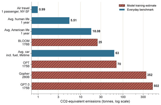
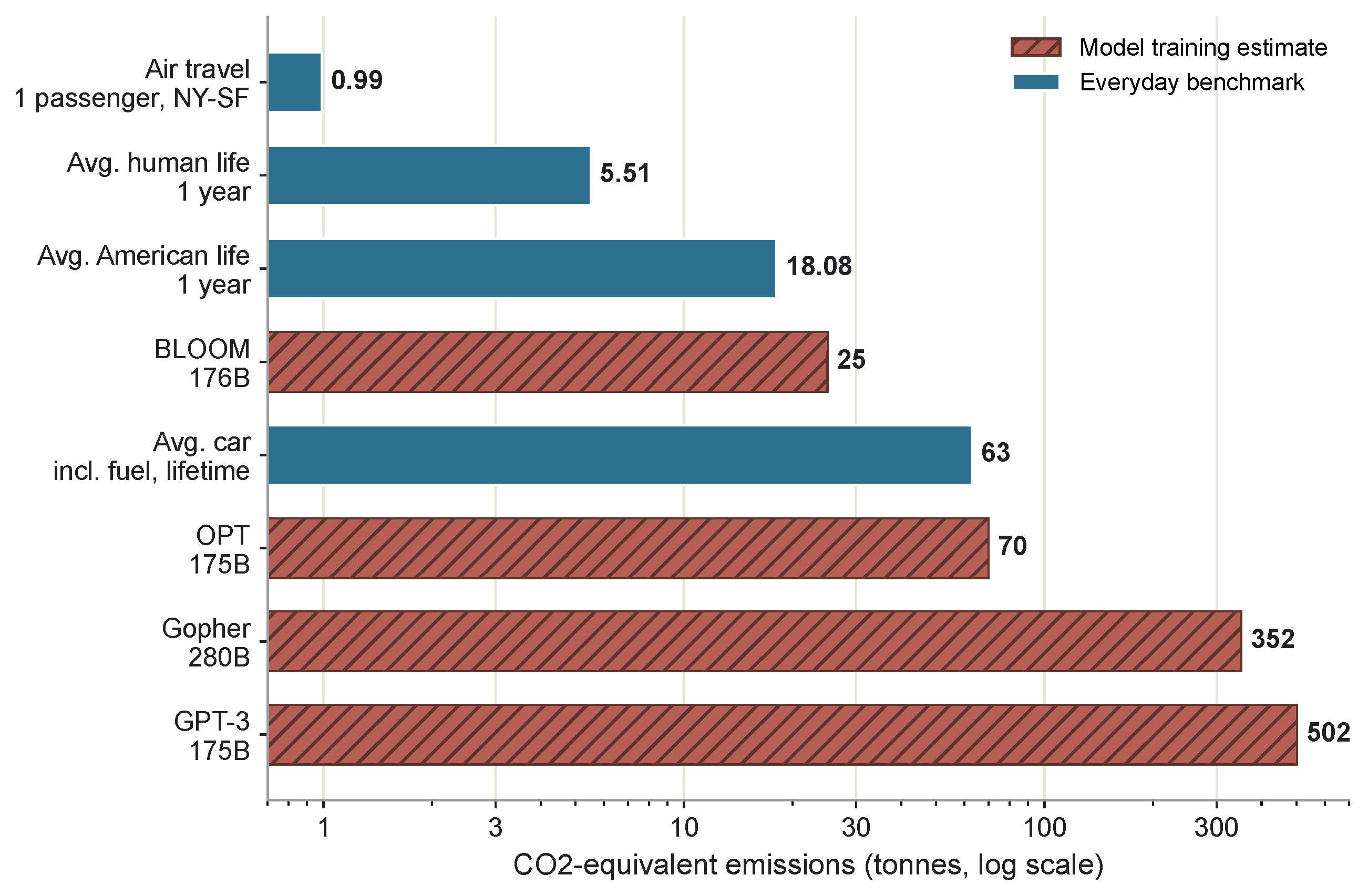
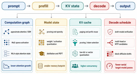
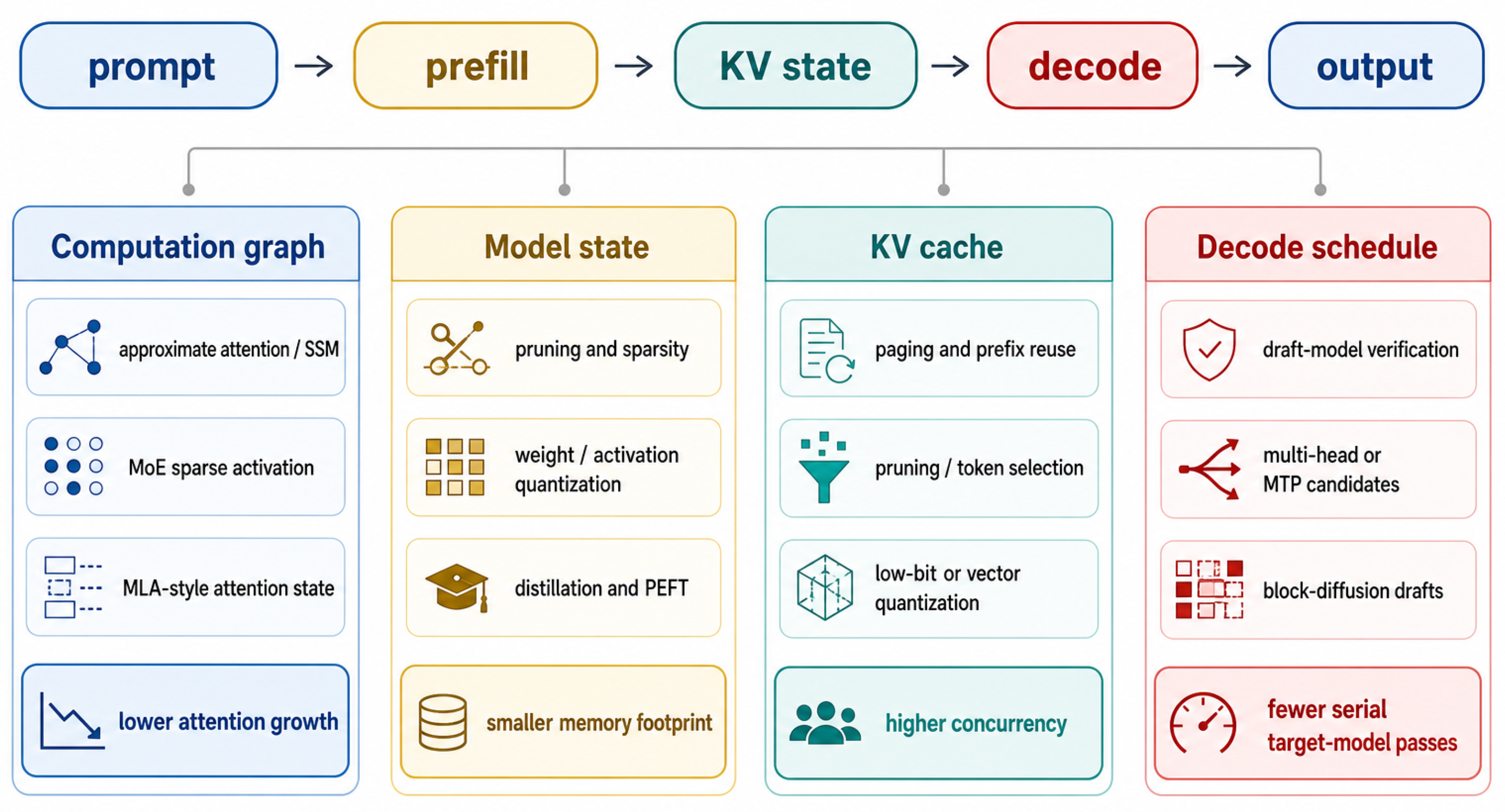
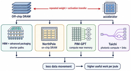
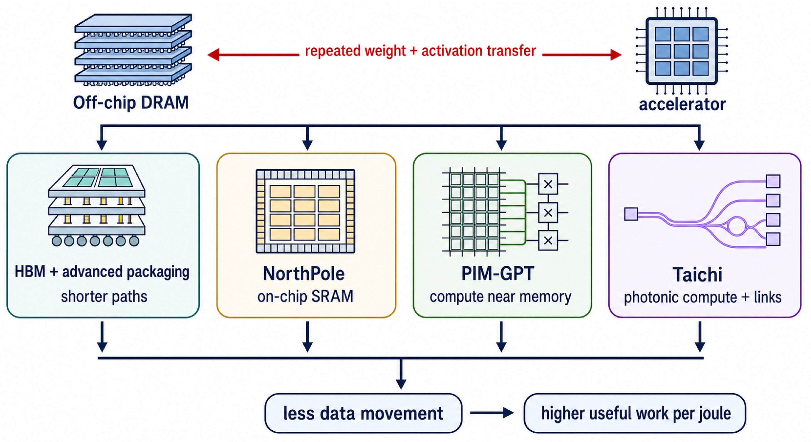
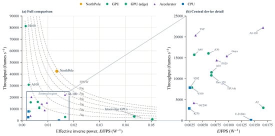
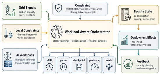
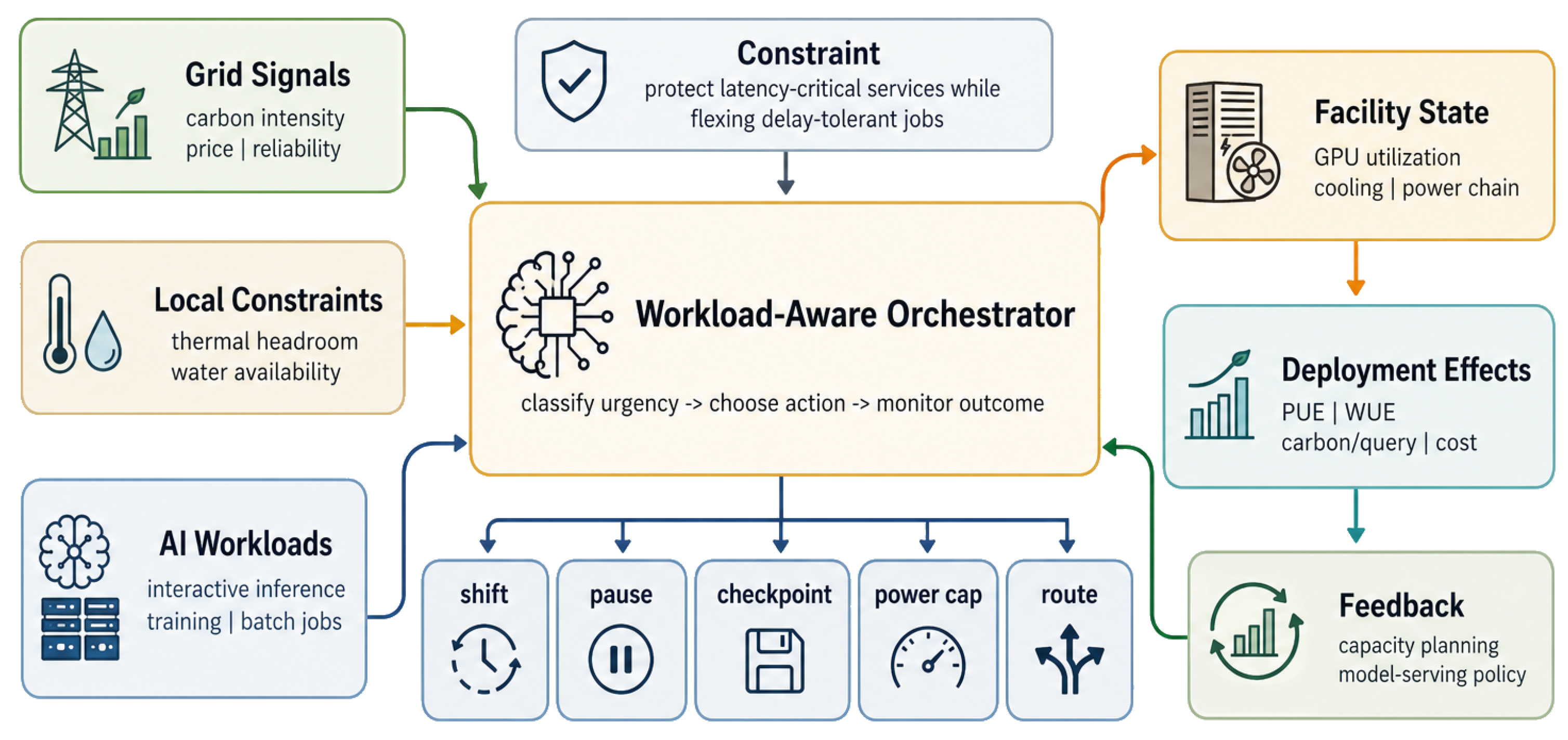
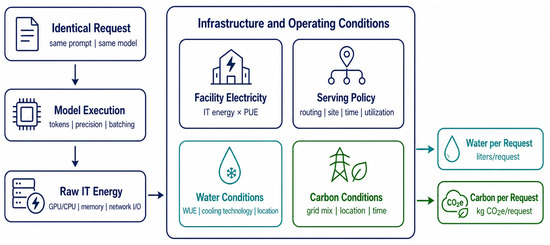
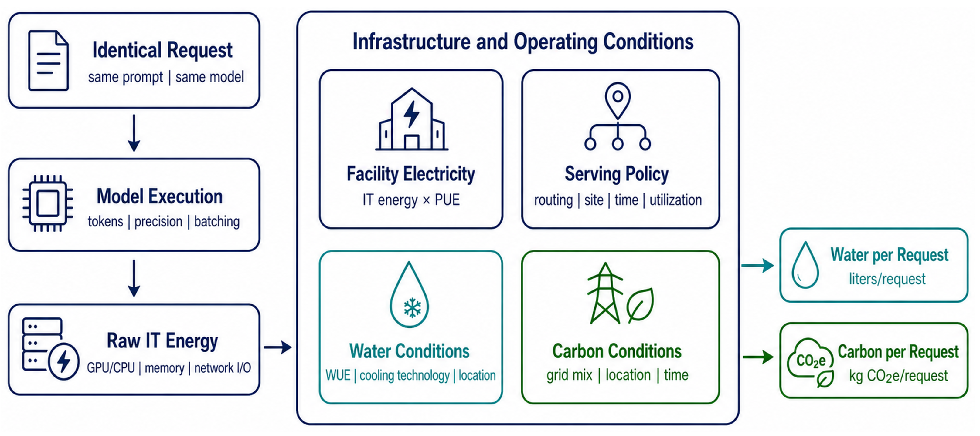
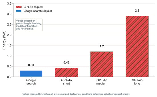
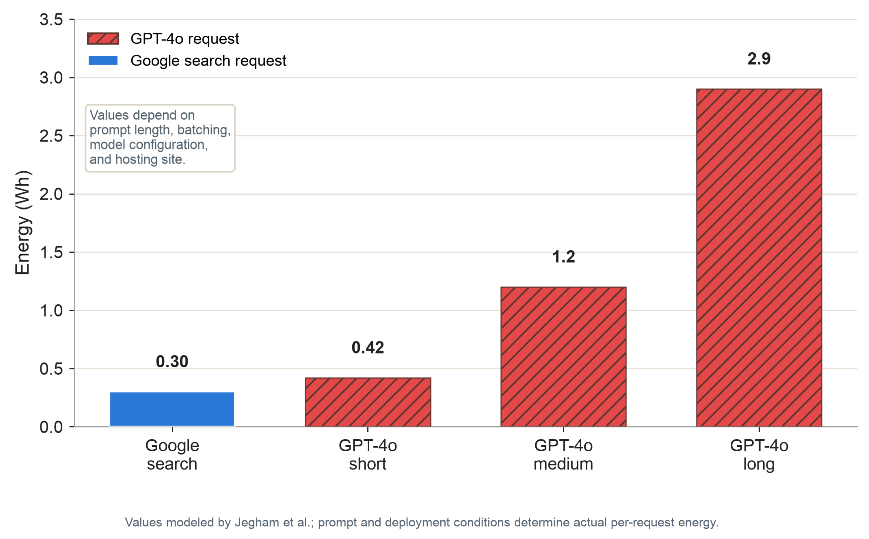

Disclaimer/Publisher’s Note: The statements, opinions and data contained in all publications are solely those of the individual author(s) and contributor(s) and not of MDPI and/or the editor(s). MDPI and/or the editor(s) disclaim responsibility for any injury to people or property resulting from any ideas, methods, instructions or products referred to in the content. |
© 2026 by the authors. Licensee MDPI, Basel, Switzerland. This article is an open access article distributed under the terms and conditions of the Creative Commons Attribution (CC BY) license.