


Simple Summary
Computer models that help diagnose cancer or predict survival must learn from patients whose outcome is known. Confirming a diagnosis or waiting years for an outcome is costly, so many records lack this information. Methods that also learn from such unlabeled records are often proposed. We tested whether they help, using four public breast cancer datasets in which the outcomes of 50% to 90% of the training cases were hidden. Each method was compared with the same model trained on labeled cases, with both using preprocessing fitted on all training cases. Under the tested settings, we found no statistically significant additional benefit from unlabeled cases beyond shared preprocessing, although potentially useful gains remain uncertain; at the standard decision threshold, some methods detected fewer positive cases. A general-purpose model pretrained on millions of artificial datasets and supplied with labeled cases after shared preprocessing achieved the highest precision–recall performance in every setting. These results support including it as a reference model when evaluating methods with limited labels.
Abstract
Background/Objectives: Machine learning for cancer diagnosis and prognosis requires costly patient labels. Semi- and self-supervised methods exploit unlabeled data but are rarely tested against equivalent supervised models. We tested whether unlabeled data help and compared these methods with a tabular foundation model. Methods: Four public breast cancer datasets (WDBC, Mammography, METABRIC, SEER) crossed clinical task (diagnosis, including the detection of microcalcifications on Mammography, or prognosis) with class balance. In five-fold cross-validation with five seeds, 10%, 20%, or 50% of training records were labeled. Self-training (random forest and XGBoost), label spreading, and SCARF self-supervised pretraining were each compared with a matched supervised control; logistic regression and TabPFN v2 were references. Analyses used corrected resampled t-tests with Holm adjustment, Bayesian correlated and hierarchical tests, and power analysis. Results: Of 96 comparisons with matched controls in the Matthews correlation coefficient (MCC) and the area under the precision–recall curve (PR-AUC), three were significant, all involving SCARF: two losses on Mammography and one PR-AUC gain on METABRIC that persisted with all labels. The estimated minimum detectable effects at 80% power varied across comparisons, with medians of approximately 0.06 in PR-AUC and 0.09 in MCC; the median absolute observed differences were 0.008 and 0.015, respectively. At the default threshold and 10% labels, label spreading lowered sensitivity on SEER (−0.135) and random-forest self-training on Mammography (−0.122). TabPFN had the highest PR-AUC in all 16 settings. Conclusions: Under the evaluated datasets, methods and settings, no statistically significant additional benefit from unlabeled data beyond shared preprocessing was detected, but the evidence does not establish equivalence; TabPFN achieved the highest PR-AUC in every setting. New methods should be tested against matched controls and tabular foundation models with adequate power.
1. Introduction
Machine learning models built on clinical, pathological and molecular variables can support both the diagnosis and the prognosis of cancer [1,2]. Training them requires labeled patients, and in oncology, labels are costly. A diagnostic label usually rests on pathological confirmation, and a prognostic label on long follow-up: a 10-year survival label cannot be assigned to a patient who is alive and was diagnosed less than 10 years ago. Clinical databases therefore often hold far more unlabeled than labeled patients [3], a situation known as label scarcity.
Two families of methods aim to learn from these unlabeled patients. Semi-supervised learning trains on labeled and unlabeled patients together [4]. In self-training, a model assigns pseudo-labels to the unlabeled patients it is confident about and is retrained on them [5]; in label spreading, labels propagate over a graph that links similar patients [6]. Self-supervised learning first learns a representation from unlabeled patients, for example, by reconstructing masked features or by matching corrupted views of the same patient, and then fine-tunes it on the labeled patients [7,8,9].
These methods have shown promise on tabular data. SCARF (self-supervised contrastive learning using random feature corruption) improved classification on 69 benchmark datasets, also when only a quarter of the training labels were available [9]. VIME (value imputation and mask estimation) outperformed supervised models in predicting prostate cancer treatment [7]. In oncology, semi-supervised learning has been reported to improve the prediction of colorectal cancer recurrence from gene expression [10] and of survival from incomplete clinical data [11]. Across 90 tabular benchmark datasets, an autoencoder-based semi-supervised method outperformed its supervised counterpart, particularly when labels were scarce, and class imbalance was among the dataset properties associated with its gains [12]. Other methods learn few-shot tasks from unlabeled tables [13] or refine self-training for tabular data [14].
Unlabeled data do not always help by default, however. Semi-supervised learning can perform worse than learning from the labeled data alone [15], and self-training can reinforce its own early errors, a problem known as confirmation bias [16]. Under class imbalance, which is common in cancer data and is often addressed by resampling, including synthetic oversampling with generative adversarial networks [17], pseudo-labels are biased toward the majority class [18,19]; when the minority class is the disease, this bias means missed cases. On tabular data, tree ensembles also remain strong baselines that deep and pretrained models often fail to beat [20,21,22]. A review of semi-supervised learning in cancer diagnostics noted that few studies reported comparisons with supervised baselines and cautioned that the approach is not a silver bullet [3].
Tabular foundation models offer a different route to learning from few labels. TabPFN (tabular prior-data fitted network) is a transformer pretrained on millions of synthetic datasets; it predicts for new patients by conditioning on the labeled training patients, without being trained on the task [23,24]. Its second version outperformed previous methods on datasets with up to 10,000 samples [24]. It has also begun to be used for clinical prediction, for example, of lymphovascular invasion in breast cancer [25] and of the outcome of non-invasive ventilation [26]. Comparing these methods with TabPFN tests whether they outperform a strong reference model that conditions on labeled patients; the matched-control comparisons separately assess the additional contribution of unlabeled patients.
How methods are compared matters as much as which methods are compared. Realistic evaluations compare each method with the same model trained on the labeled data alone, so that the contribution of the unlabeled data is not confused with differences between models [27]. Repeated cross-validation runs share patients, so tests that treat them as independent overstate significance [28,29], and conclusions drawn from a single random seed can be unreliable [30]. Clinical use also depends on sensitivity and specificity, which show how many cancers are missed and how many false alarms are raised, and which summary measures such as accuracy or the area under the receiver operating characteristic curve (ROC-AUC) do not reveal.
Class imbalance is a well-studied problem in cancer prediction, and resampling techniques combined with machine learning models have been shown to improve the detection of the minority class in both diagnosis and prognosis [31]. Missing labels, by contrast, have received far less attention, although they are just as common in clinical data. Label scarcity and class imbalance often occur together in oncology, so we study the first while keeping the second as a design factor. We define label scarcity as having labels for only 10%, 20% or 50% of the training patients and address four research questions:
- RQ1. Do methods that learn from unlabeled patients (self-training, label spreading and SCARF self-supervised pretraining) outperform matched supervised controls trained on the same labeled patients?
- RQ2. Does any benefit or harm depend on the clinical task (diagnosis or prognosis) or on class imbalance?
- RQ3. How do these methods change sensitivity and specificity, and hence the numbers of missed cases and false alarms?
- RQ4. How do they compare with a tabular foundation model, TabPFN v2, using labeled patients only?
To answer these questions, we compared ten methods on four public breast cancer datasets that cross clinical task with class balance: The Wisconsin Diagnostic Breast Cancer (WDBC) and Mammography datasets for diagnosis and the Molecular Taxonomy of Breast Cancer International Consortium (METABRIC) and Surveillance, Epidemiology, and End Results (SEER) datasets for prognosis, with one balanced and one imbalanced dataset per task. Each method that learned from unlabeled patients was paired with a supervised control that used the same model, settings, and labeled patients, and all methods shared the same 25 cross-validation splits. This study makes four contributions. It provides a controlled comparison of self-training, label spreading, and SCARF pretraining, each against a matched supervised control at three levels of label scarcity, with TabPFN v2 as a reference; all methods share preprocessing fitted on the full training fold. It adds a control that separates the effect of SCARF pretraining from the contribution of the unlabeled patients. It reports an explicit analysis of statistical power and practical equivalence, showing which effects the design could detect and how naive tests and single seeds would have changed the conclusions. Finally, it shows how each method shifts sensitivity and specificity at the default decision threshold.
2. Materials and Methods
All ten methods were trained and tested on the same cross-validation splits, labeled patients, and input features. Each method that learned from unlabeled patients was compared with a supervised control that used the same model, settings, and labeled patients (Figure 1).
Figure 1.
Study design. Four public datasets cross clinical task and class balance (n, patients analyzed; ratio, positive to negative). In each of the 25 splits, nested labeled subsets of 10%, 20% and 50% are drawn from the training fold, and the remaining training patients form the unlabeled pool. Each method that learns from unlabeled patients is compared with a control that uses the same model, settings and labeled patients; logistic regression (LR) and TabPFN v2 serve as references. SCARF-FT, SCARF pretraining followed by fine-tuning; Sup-NN, supervised neural network; ST-RF and ST-XGB, self-training with a random forest (RF) or XGBoost (XGB); LS, label spreading; LS-Sup, label spreading on a graph of labeled patients only; MCC, Matthews correlation coefficient; PR-AUC and ROC-AUC, areas under the precision–recall and receiver operating characteristic curves; RQ, research question; ROPE, region of practical equivalence.
2.1. Study Design
The four datasets cross two factors, clinical task and class balance. WDBC (cytological diagnosis of breast masses) and Mammography (detection of microcalcifications on mammograms) are diagnostic tasks, and METABRIC and SEER are prognostic. WDBC and METABRIC, with positive-to-negative ratios of 1:1.7 and 1:1.85, are only mildly imbalanced and are called balanced below, whereas SEER (1:6.02) and Mammography (1:29.9) are imbalanced. This 2 × 2 design allows an exploratory comparison across tasks and levels of imbalance (RQ2); with one dataset per cell, these factors are confounded with other properties of the datasets (Section 4.5).
We simulated label scarcity by hiding the labels of most training patients. In each training fold, labels were kept for 10%, 20%, or 50% of the patients, and the remaining patients formed the unlabeled pool; a fourth setting with all labels (100%) served as a reference. Every method was run on the same 25 cross-validation splits at each label ratio (Section 2.3). For readability, general statements call the records of all four datasets patients; Mammography records are image samples rather than patients, and we call them samples when describing that dataset alone (Section 2.2).
2.2. Datasets
The four public datasets range from 569 to 7849 patients, and at the 10% label ratio a training fold held only 16 to 41 labeled positive patients (Table 1).
Table 1.
Characteristics of the four datasets after exclusions. Ratio is positive to negative. The last column gives the number of labeled patients per training fold at the 10% label ratio, with labeled positives in parentheses; ranges cover the 25 splits.
WDBC. The Wisconsin Diagnostic Breast Cancer dataset contains 569 fine-needle aspirates of breast masses, 212 malignant and 357 benign [32,33]. Its 30 numeric features are the mean, standard error and worst value (mean of the three largest) of ten cell-nucleus characteristics measured on digitized images. It has no missing values or duplicate records.
Mammography. This dataset (OpenML ID 310) contains 11,183 samples from mammograms, 260 of them microcalcifications, described by six numeric image features that are standardized in the distributed file [34,35]. The task is the detection of microcalcifications, which can be an early sign of breast cancer, rather than the diagnosis of cancer itself. We removed 3334 exact duplicate rows with identical features and class, so that the same record could not appear in both a training and a test fold; 3327 of them repeated a single feature vector with all six features at their minimum. This left 7849 samples, 254 of them positive. The file has no patient or image identifiers, so samples could not be grouped by patient during cross-validation.
METABRIC. We used the clinical data of the METABRIC cohort distributed by cBioPortal (study brca_metabric, 2509 patients) [36,37,38,39]. Before analysis, 524 patients without overall survival data (survival time, survival status, and vital status) were removed, leaving 1985; these patients also lacked 13 of the 26 features used here, including all treatment variables and molecular subtypes. The target was death from breast cancer within 10 years (120 months); the negative class comprised patients followed for more than 120 months, including 131 who died of breast cancer later. We excluded 267 patients alive with 120 months or less of follow-up, whose 10-year outcome is unknown, and 245 who died of other causes within 120 months, a competing risk. Counting these 245 patients as negatives would have changed the target to include competing deaths as non-events, with a positive rate of 30.0% rather than 35.1%. All methods were evaluated on the same selected cohort, but their relative performance may depend on this outcome definition and exclusion rule. Four patients with no recorded outcome were also excluded, leaving 1469 patients, 515 of them positive. The 26 features (7 numeric, 19 categorical) covered age at diagnosis and inferred menopausal state; tumor size, stage, histological grade, cellularity, laterality and histological type (four variables, including the Oncotree code); the number of positive lymph nodes and the Nottingham prognostic index; estrogen (two measurements), progesterone and human epidermal growth factor receptor 2 (HER2) status; molecular variables (PAM50 and claudin-low subtype, integrative cluster, 3-gene classifier subtype, HER2 status measured by single-nucleotide polymorphism (SNP) 6.0 arrays, and mutation count); and treatments received (type of surgery, chemotherapy, hormone therapy and radiotherapy). Survival and relapse variables, the patient identifier, the cohort number, and sex, which was female for all patients, were excluded. The molecular and treatment variables are not all available at diagnosis; they were kept because the study compares learning methods rather than proposing a deployable model, and all methods received the same features. Of the analyzed patients, 638 had at least one missing value (969 values in total). Because treatments and some molecular variables become available only after diagnosis, the METABRIC task is a retrospective benchmark of prognostic modeling rather than prediction at the time of diagnosis (Section 4.5).
SEER. This extract from the November 2017 release of the SEER Program contains 4024 women with infiltrating duct and lobular carcinoma diagnosed in 2006–2010 [40]. The provider had excluded patients with unknown tumor size or unknown numbers of examined or positive regional lymph nodes, and those who survived less than one month. Because the extract does not record the cause of death, the target was death from any cause within 5 years (60 months); the negative class comprised patients followed for more than 60 months, including 158 who died later. After removing one duplicate row, we excluded 807 patients alive with 60 months or less of follow-up, leaving 3216 patients, 458 of them positive. Unlike a previous study of these data, which used the vital status at last contact as the target [31], the fixed horizon does not count patients censored before 60 months as survivors. The 13 features were age, tumor size, the numbers of examined and positive regional lymph nodes, race, marital status, T stage, N stage, American Joint Committee on Cancer (AJCC) 6th edition stage, grade, SEER historic stage A, and estrogen and progesterone receptor status; none had missing values. Survival time and vital status defined the target and were not used as features.
2.3. Cross-Validation and Label Scarcity
Each dataset was split by stratified five-fold cross-validation repeated with five random seeds (42–46), giving 25 train–test splits. Within each training fold, a stratified random sample formed the labeled subset: its size was the training-fold size multiplied by the label ratio (10%, 20%, or 50%) and rounded down, and it was divided among the classes in proportion to their frequencies, again rounding down within each class. The subsets were nested (each smaller subset was contained in the larger ones), were drawn once per split and were shared by all methods; at 100%, all training patients were labeled.
The remaining training patients formed the unlabeled pool, whose labels were hidden from every method. The test fold was never used for pretraining, pseudo-labeling, graph construction, or preprocessing.
Preprocessing was fitted in each split on all training-fold patients, without labels, and then applied to the test fold. Numeric features were imputed with the median. Categorical features were imputed with the most frequent category and ordinally encoded, with categories unseen in training coded as −1, and all methods treated these codes as numbers. All features were then standardized to zero mean and unit variance. Because it used no labels, preprocessing was shared by all methods; beyond it, the features of unlabeled patients entered only the four methods designed to use them. This setting corresponds to deployment in which the unlabeled records are available at training time, as in a hospital that holds many records without confirmed outcomes; test-fold patients were never used. As a sensitivity analysis, we repeated the experiments on METABRIC and SEER, the only datasets with categorical features, with one-hot encoding (one 0/1 column per category and one column for binary features), keeping the splits, labeled subsets, seeds, models and settings unchanged. This analysis covered self-training, label spreading and their controls; SCARF-FT, Sup-NN and TabPFN were not repeated because of their computational cost on CPUs.
2.4. Methods and Matched Controls
The four methods that learned from unlabeled patients represent three common families: self-supervised pretraining, self-training, and graph-based label propagation. Each was paired with a supervised control that used the same model, settings, seeds and labeled patients, with no use of unlabeled patients beyond shared preprocessing.
- SCARF-FT versus Sup-NN. SCARF-FT pretrains a neural network encoder on all training-fold patients with SCARF, a self-supervised contrastive method for tabular data [9], and then fine-tunes it on the labeled patients. Sup-NN trains the same network from random initialization on the labeled patients.
- ST-RF versus RF and ST-XGB versus XGB. Self-training [5] repeatedly adds unlabeled patients with confident predictions, labeled with the predicted class (pseudo-labels), to the training data of a random forest (RF) [41] or XGBoost (XGB) [42]. The controls are the same models trained on the labeled patients alone.
- LS versus LS-Sup. Label spreading (LS) [6] propagates labels over a nearest-neighbor graph of all training-fold patients. LS-Sup builds the same graph from the labeled patients only.
Two methods that use labeled patients after shared preprocessing served as references: logistic regression (LR), a standard clinical baseline, and TabPFN v2 [24]. TabPFN is a tabular foundation model, a transformer pretrained on millions of synthetic datasets, which predicts by conditioning on the labeled patients in a single forward pass, without updating its weights.
At 100% labels, no unlabeled patients remain, so ST-RF, ST-XGB and LS must reproduce their controls exactly. They did so for every metric in all 25 runs on every dataset, confirming that without unlabeled patients each method was identical to its control. SCARF-FT still differs from Sup-NN at 100% because of pretraining, so this difference measures the effect of pretraining without unlabeled patients (Section 2.8).
2.5. Model Settings
Settings were fixed before the final runs and were identical across datasets and label ratios. No hyperparameters were tuned, and no validation data or early stopping were used, so the test folds served only for evaluation. Fixed settings were chosen deliberately: each method shared its model and settings with its matched control, so the comparison isolates the use of unlabeled patients, and at 10% labels the labeled subsets (44 patients with 16 positives on WDBC and 20 positives on Mammography; Table 1) would leave validation sets too small for reliable tuning [27].
Neural networks. SCARF-FT and Sup-NN share one architecture: an encoder with two hidden layers of 128 units, each followed by batch normalization [43] and a rectified linear unit (ReLU) activation, then a 64-unit output layer, topped by a linear classification layer. For SCARF pretraining, a corrupted view of each patient was created by replacing each feature, with probability 0.6, by a value drawn from that feature’s empirical marginal distribution among the training-fold patients. The encoder and a projection head (one hidden layer of 64 units, 32 outputs) were trained with the InfoNCE contrastive loss [44] at temperature 1. This loss pulls together the original and corrupted views of each patient and pushes apart those of different patients in the batch. The corruption rate and temperature are the defaults recommended by the SCARF authors [9].
Pretraining used Adam [45] with learning rate 10−3 and weight decay 10−4, cosine learning-rate decay [46], batch size 64 and 200 epochs. It ran once per split, and the pretrained encoder was reused at every label ratio. For fine-tuning, the projection head was discarded and the whole network was trained on the labeled patients with full-batch Adam (learning rate 10−4, weight decay 10−4) for 300 epochs. Sup-NN followed the same fine-tuning procedure, with the same seed, from random initialization.
Tree ensembles and self-training. RF used 500 trees; all other RF and XGB settings were library defaults. Self-training used the SelfTrainingClassifier of scikit-learn. In each round, the current model pseudo-labeled every unlabeled patient whose highest predicted class probability exceeded 0.8, and the model was refitted on the labeled and pseudo-labeled patients. Self-training stopped after 10 rounds, or earlier when no further unlabeled patient qualified. Pseudo-labels were selected by confidence alone, without class-balanced selection. RF recomputed its balanced class weights at each round from the labeled and pseudo-labeled patients, whereas the positive-class weight of XGB stayed at the value computed from the labeled patients. For each run, we recorded how many unlabeled patients were pseudo-labeled and how many of these pseudo-labels matched the hidden labels (Section 3.7).
Label spreading. LS and LS-Sup used the LabelSpreading implementation of scikit-learn with a k-nearest-neighbor graph (k = 7), clamping factor α = 0.2 and at most 30 iterations, the library defaults. A test patient received class probabilities from its seven nearest training patients. If label spreading had reached none of these neighbors, scikit-learn returned undefined probabilities, and we assigned the class frequencies of the labeled patients instead, which gives a probability of 0.5 after the balancing described below. This happened only for LS: on SEER, for 1.5 of about 644 test patients per split at 10% labels (at most 19) and 0.2 at 20%, and on Mammography, for 0.4 of about 1570 at 10% (at most 6).
Reference methods. LR used L2 regularization with C = 1, balanced class weights and up to 5000 iterations. TabPFN used the version 2 model weights with ModelVersion V2 selected explicitly and balance_probabilities = True and received the labeled patients as its training data. We used version 2 for three reasons. It is described in a peer-reviewed publication [24], whereas later versions are described in technical reports [47,48]. It was pretrained only on synthetic data, so the public datasets used here were not part of its training data. Its weights are distributed under an Apache 2.0-based license that permits commercial use, whereas later versions have non-commercial model licenses under which use in practice requires a commercial license [49]; we therefore preferred a reference that clinical teams can adopt. We lifted the package’s default limit of 1000 training samples on a central processing unit (CPU), which would otherwise have blocked the larger labeled subsets.
Class imbalance. Every method was cost-sensitive. In training, the neural networks, LR, RF, and XGB gave both classes equal total weight: the neural networks and XGB weighted positive patients by the ratio of negative to positive labeled patients, and LR and RF used balanced class weights. LS and LS-Sup divided their predicted probabilities by the class frequencies of the labeled patients and renormalized them, and TabPFN rebalanced its probabilities with its built-in option. Resampling and balanced ensemble learning are common alternatives for imbalanced biomedical prediction tasks [50]. We used class weighting instead, so that every method saw the same patients and the comparisons with unlabeled patients were not confounded by synthetic or duplicated records. No resampling was used, and all methods predicted the positive class when its probability was at least 0.5.
2.6. Evaluation Metrics
Predicted probabilities for each test fold were scored against the positive class defined in Table 1. The primary metric was the Matthews correlation coefficient (MCC) [51], which uses all four cells of the confusion matrix and remains informative under class imbalance [52]. The area under the precision–recall curve (PR-AUC), computed as average precision, summarizes precision and recall over all thresholds and is more informative than ROC-AUC on imbalanced data [53]. Its no-skill value equals the share of positive patients: 0.373 for WDBC, 0.032 for Mammography, 0.351 for METABRIC, and 0.142 for SEER.
We also report ROC-AUC, sensitivity, and specificity. Sensitivity and specificity determine the shares of missed cases (one minus sensitivity) and false alarms (one minus specificity) addressed by RQ3. MCC, sensitivity, and specificity were computed at the 0.5 threshold. Macro-averaged F1, weighted F1, and accuracy are reported in Table S1. Each metric was computed on every test fold and summarized as the mean and standard deviation (SD) over the 25 runs.
2.7. Statistical Analysis
All comparisons were paired. For each of the 25 runs, we took the difference between two methods on the same test fold, labeled subset and seed; for RQ1–RQ3, this was a method minus its control. Because the training sets of the 25 runs overlap, these differences are correlated, and the standard paired t-test underestimates their variance. We therefore used the corrected resampled t-test [29,54]:
where and are the mean and variance of the J = 25 differences, and ntest/ntrain = 1/4 in five-fold cross-validation. The statistic was compared with a t distribution with 24 degrees of freedom, and 95% confidence intervals (CIs) used the same standard error. The correction assumes the overlap between training sets of standard cross-validation; because the methods were trained on labeled subsets of 10–50% of each training fold, we also repeated the tests with the ratio of the test-fold size to the labeled-subset size (0.5 to 2.5), a more conservative variant (Section 3.8).
Holm’s procedure [55] controlled the family-wise error rate at 0.05 within each dataset and metric. For RQ1–RQ3, a family held the 12 comparisons of the four pairs at the three label ratios and was tested for MCC, PR-AUC, and sensitivity; specificity differences were descriptive. For RQ4, a family held the 36 comparisons of the other nine methods with TabPFN at the four label ratios, tested for PR-AUC, ROC-AUC, and MCC. The SCARF-FT−Sup-NN difference at 100% labels was tested separately without adjustment.
A non-significant result does not show that two methods are equivalent, so we also applied the Bayesian correlated t-test [56,57]. Its posterior for the mean difference is a Student’s t distribution with 24 degrees of freedom, centered on and scaled by the corrected standard error. We report the posterior probabilities that a method was better, practically equivalent or worse, with a region of practical equivalence (ROPE) of ±0.01 and, as a sensitivity analysis, ±0.02 and ±0.03. For each comparison, we also counted wins and losses over the 25 runs and the number of seeds, of five, with a positive or negative mean difference. To answer RQ1 across datasets, we also fitted the Bayesian hierarchical model of Corani et al. [58] to the paired differences of all four datasets, separately for each pair, label ratio, and metric. The model treats the mean differences of the datasets as draws from a common Student’s t distribution and accounts for the correlation between cross-validation runs, with the correlation set to ρ = 1/5 for five-fold cross-validation (five runs of five folds). We report the posterior mean of the average difference across datasets with its 95% credible interval, and the posterior probabilities that a gain, practical equivalence (ROPE ±0.01), or a loss is the most probable outcome on a new dataset. We used the Stan model and default priors of baycomp 1.0.3, run in PyStan 3.14 with four chains of 10,000 draws.
To characterize statistical sensitivity, we estimated for each comparison an approximate minimum detectable effect at 80% power as (t_Holm + t_0.80) × SE, using the observed corrected standard error and the first Holm threshold (Section 3.9). Here SE is the corrected standard error, t_0.80 = 0.86, and t_Holm = 3.17 is the critical value of the first Holm step for 12 tests with 24 degrees of freedom.
Methods were also ranked by their mean MCC, PR-AUC, and ROC-AUC in each of the 16 dataset–label-ratio settings. Because settings within a dataset share patients, mean ranks are reported descriptively, without a significance test.
As a sensitivity analysis (Section 3.8), we repeated the RQ1 tests with two procedures that treat the 25 runs as independent, the Wilcoxon signed-rank test [59] and the uncorrected paired t-test, using the same Holm families, and examined each seed separately. Five seeds balanced stability against computing time: more seeds would add little power, because the variance factor of the corrected test, 1/J + 1/4, cannot fall below 1/4 however many repetitions are added [29,60].
2.8. Pretraining Decomposition Control
SCARF-FT differs from Sup-NN in two ways, pretraining and the use of unlabeled patients, so we added a control to separate them. SCARF-FT-Lab pretrained SCARF on the labeled patients only, also drawing its corruption values from them, and was otherwise identical to SCARF-FT, including seeds and fine-tuning. The total effect then splits into two additive parts:
If a training fold had fewer than 64 labeled patients, the pretraining batch held all of them; this applied only to WDBC at 10% labels (44 patients). At 100% labels, SCARF-FT-Lab equals SCARF-FT by definition. Each component was tested with the corrected resampled t-test, with Holm adjustment over the 12 dataset–label-ratio settings for each component and metric (MCC and PR-AUC).
The control was run on a second computer with the same library versions, where SCARF-FT and Sup-NN were rerun so that all three models came from one run. The total effect agreed with the main experiment to within 0.011 MCC in every setting; such small differences are expected because neural network training is not bit-for-bit reproducible across computers. Because this difference is of the same order as the smaller components, components below about 0.01 were not interpreted individually.
2.9. Implementation and Reproducibility
The experiments were implemented in Python with scikit-learn 1.9.1 [61], XGBoost 3.4.1, PyTorch 2.14.1 [62], TabPFN 9.2.0, NumPy 2.5.3, pandas 3.0.5 and SciPy 1.18.1, and all models ran on CPUs. The main experiments ran under Windows with Python 3.12, and the decomposition control under Linux with Python 3.13. We pinned the library versions because random forest and XGBoost results differed between library versions in preliminary runs; such tool and version issues are common in data science [63]. Seeds were fixed for every split, labeled subset and model, so all methods saw identical data. During development, single-seed runs (seed 42) on WDBC and METABRIC were used to test the code and to fix the library versions; the set of methods and the prognostic targets were finalized after these runs, no setting was tuned on them, and the final analysis used all five seeds, including seed 42.
3. Results
No statistically significant additional benefit from unlabeled patients beyond shared preprocessing was detected on any dataset at any label ratio; the estimated minimum detectable effects varied across comparisons, with medians of approximately 0.06 in PR-AUC and 0.09 in MCC (Section 3.9). TabPFN, using labeled patients only, had the highest PR-AUC in all 16 dataset–label-ratio settings. Section 3.1 summarizes overall performance. Section 3.2 and Section 3.3 answer RQ1, and Section 3.4, Section 3.5 and Section 3.6 answer RQ2, RQ3 and RQ4, respectively. Section 3.7, Section 3.8 and Section 3.9 report pseudo-label diagnostics, the effect of the choice of statistical test and number of seeds, and statistical power. Effects are mean paired differences over the 25 runs (5 seeds × 5 folds). Unless stated otherwise, p values come from the corrected resampled t-test, Holm-adjusted within each dataset and metric.
3.1. Overall Performance
Performance differed far more between datasets than between methods (Table 2). WDBC was close to the ceiling: MCC ranged from 0.780 to 0.888 at 10% labels and from 0.916 to 0.949 with all labels, and PR-AUC stayed above 0.91. Prognosis was harder, with a best MCC of 0.360 on METABRIC and 0.289 on SEER, both reached by TabPFN with all labels. On Mammography, the tree ensembles led on MCC (up to 0.694) and LR trailed (0.377–0.417).
Table 2.
Mean MCC over 25 runs (5 seeds × 5 folds) by dataset, proportion of labeled training patients and method. Datasets are ordered by task (diagnosis, then prognosis), with the balanced dataset first within each task. Bold marks the best value in each row. At 100% labels, ST-RF, ST-XGB and LS coincide with RF, XGB and LS-Sup by construction. Mean rank is averaged over the 16 rows (1 = best). Table 3 gives standard deviations and all five metrics at 10% labels, and Table S1 at every label ratio.
Table 3 reports all five metrics for every method at 10% labels, the scarcest setting, where most training patients were unlabeled.
Table 3.
Classification performance at 10% labels: mean ± SD over 25 runs (5 seeds × 5 folds). Datasets are ordered by task (diagnosis, then prognosis), with the balanced dataset first within each task. Bold marks the best MCC, PR-AUC, and ROC-AUC for each dataset; sensitivity and specificity trade off against each other and are not ranked. Results at every label ratio, together with macro-F1, weighted F1 and accuracy, are in Table S1.
3.2. Effect of Unlabeled Patients (RQ1)
Of the 96 comparisons in Table 4 (4 pairs × 4 datasets × 3 label ratios × 2 metrics), three were significant, all involving SCARF; the decomposition analysis did not detect a statistically significant contribution from unlabeled patients to these effects (Section 3.3). SCARF-FT lowered MCC on Mammography at 20% labels (−0.055, 95% CI [−0.089, −0.020], p = 0.034) and at 50% (−0.044, [−0.071, −0.016], p = 0.034), and raised PR-AUC on METABRIC at 50% (+0.040, [0.015, 0.065], p = 0.035). No semi-supervised method improved significantly on its control.
Table 4.
Mean paired difference between each method and its supervised control over 25 runs; for SCARF-FT, this includes both pretraining and the use of unlabeled patients, which are examined separately in Section 3.3. Positive values favor the method that used unlabeled patients. Datasets are ordered by task (diagnosis, then prognosis), with the balanced dataset first within each task. Bold: Holm-adjusted p < 0.05 (corrected resampled t-test, 12 tests per dataset and metric). Confidence intervals, unadjusted and adjusted p values, win counts, seed signs and Bayesian probabilities are in Table S2.
SCARF-FT effects in the same directions were also observed at 100% labels, showing that pretraining can produce gains or losses without additional unlabeled patients. With all labels, where SCARF-FT and Sup-NN were trained on identical patients, SCARF-FT still exceeded Sup-NN on METABRIC (PR-AUC +0.051, [0.024, 0.078], unadjusted p < 0.001; MCC +0.059, [0.005, 0.112], p = 0.033) and still trailed it on Mammography (MCC −0.054, [−0.084, −0.024], p = 0.001). The three semi-supervised methods, by contrast, reproduced their controls exactly in all 25 runs on every dataset at 100% labels, confirming that each of these pairs differs only in the use of unlabeled patients.
Several non-significant effects had the same sign in all five seeds. LS lowered PR-AUC on both prognostic datasets at 10% labels (METABRIC −0.058, SEER −0.052) and on SEER at 20% (−0.048). ST-RF lowered PR-AUC on Mammography at every label ratio (−0.034, −0.027, −0.017) and on METABRIC at 10% and 20% (−0.022 each). On WDBC, both self-training methods lowered MCC at 10% and 20% labels (−0.016 to −0.032).
The Bayesian analysis was less conclusive than the absence of significant effects might suggest (Table S2). With a ROPE of ±0.01, six comparisons were practically equivalent (posterior probability of the ROPE > 0.95), all for PR-AUC on WDBC. Six were probable gains (posterior probability > 0.95 of a gain beyond the ROPE), all for SCARF-FT on prognosis, at 50% labels on METABRIC and at 20% and 50% on SEER, for both MCC and PR-AUC; these are the two datasets on which SCARF-FT also exceeded Sup-NN with all labels. Six were probable losses, for SCARF-FT on Mammography (MCC, all three ratios) and for LS at 10% labels on METABRIC (MCC and PR-AUC) and SEER (PR-AUC), and the remaining 78 were undecided. Equivalence within ±0.01 required a standard error below about 0.005, which only seven comparisons, all for PR-AUC on WDBC, reached; at the median standard error of 0.017, the posterior probability of the ROPE could not exceed 0.44 even for a mean difference of zero. With ROPEs of ±0.02 and ±0.03, 10 and 22 comparisons were practically equivalent, one and zero were probable gains, and three and zero were probable losses, respectively.
Pooling the four datasets with the hierarchical model did not change these conclusions (Table S5). For every pair, label ratio, and metric, the 95% credible interval of the average difference across datasets included zero, with posterior means from −0.023 to +0.020, and no gain, practical equivalence, or loss reached a posterior probability of 0.95 on a new dataset. The pooled results pointed in the same directions as the per-dataset ones: a gain was the most probable outcome for SCARF-FT in PR-AUC (probability up to 0.81, at 50% labels), and a loss for LS and ST-RF in PR-AUC at 10% labels (0.79 and 0.78). With only four heterogeneous datasets, the credible intervals were wide, from 0.045 to 0.181.
3.3. Pretraining Versus Unlabeled Patients (RQ1)
The SCARF-FT effects found under RQ1 could come from pretraining itself or from the unlabeled patients in its pretraining set. The SCARF-FT-Lab control, pretrained on the labeled patients only, separates the two (Figure 2). SCARF-FT−SCARF-FT-Lab isolates the contribution of unlabeled patients, and SCARF-FT-Lab−Sup-NN isolates pretraining itself. At low label ratios, the first difference measures the mechanism through which self-supervised pretraining is expected to benefit from unlabeled patients: a larger pretraining set.
Figure 2.
Decomposition of the SCARF-FT effect on MCC into pretraining (SCARF-FT-Lab−Sup-NN) and unlabeled patients (SCARF-FT−SCARF-FT-Lab), from the control run (25 runs per bar). Whiskers show 95% confidence intervals from the corrected resampled t-test, unadjusted for multiple testing. Black ticks mark the total (SCARF-FT−Sup-NN), which differs from the main experiment (Table 4) by at most 0.011 because the neural models were rerun in a second computing environment (Section 3.3). At 100% labels, there are no unlabeled patients, so the total equals the pretraining effect. * Holm-adjusted p < 0.05 (12 tests per component) for the pretraining component; no unlabeled-patient component was significant.
No contribution of unlabeled patients was significant, either for MCC (all adjusted p = 1.00; smallest unadjusted p = 0.108) or for PR-AUC (smallest adjusted p = 0.671). Their contribution to MCC was largest when labels were scarcest: at 10% and 20% labels, it was +0.025 and +0.027 on METABRIC, +0.016 and +0.024 on SEER, +0.009 and +0.015 on WDBC, and −0.019 and −0.018 on Mammography. At these ratios, it exceeded the pretraining component on METABRIC, on SEER at 10% and on WDBC, where pretraining on the labeled patients alone contributed between −0.018 and +0.004; on Mammography, both components were negative. At 50% labels, it ranged from −0.002 to +0.013.
With more labels, pretraining itself dominated. At 50% labels, it added +0.047 MCC on METABRIC and +0.053 on SEER (unadjusted p = 0.079 and 0.078), and on Mammography it lowered MCC at every ratio (−0.036, −0.035 and −0.041; adjusted p = 0.023 at 50%). On WDBC it ranged from −0.018 to +0.003 across all label ratios. PR-AUC showed the same division. On METABRIC at 50% labels, where SCARF-FT significantly exceeded Sup-NN (+0.040), pretraining contributed +0.027 and unlabeled patients +0.012, neither significantly; at 10% labels, the PR-AUC gains on METABRIC (+0.018) and Mammography (+0.016) came almost entirely from the unlabeled patients (+0.016 and +0.017). The estimated contribution of unlabeled patients was generally larger at lower label ratios, but these estimates were small and none was statistically significant.
For this control, the three neural models were rerun in a second computing environment with the same library versions. The totals (SCARF-FT−Sup-NN) reproduced the main runs within 0.011 MCC. This difference is of the same order as the smaller components, which should therefore not be interpreted individually.
3.4. Dependence on Task and Class Balance (RQ2)
For RQ2, the effects of unlabeled patients differed between the prognostic and the diagnostic datasets (Table 4), but with one dataset per combination of task and class balance, this comparison is exploratory. On both prognostic datasets, SCARF-FT numerically exceeded Sup-NN at every label ratio (MCC +0.023 to +0.058), and LS fell below LS-Sup at every ratio (MCC −0.006 to −0.073). On the diagnostic datasets, no method gained significantly; the largest MCC gain was +0.024, for LS on Mammography at 10% labels. On WDBC, where MCC ranged from 0.780 to 0.888 with 10% labels, all 12 MCC effects lay within ±0.032. On Mammography, SCARF-FT and ST-RF had lower MCC than their controls at every label ratio.
Self-training with RF lowered sensitivity substantially only on the two imbalanced datasets, by up to 0.122 on Mammography and 0.047 on SEER, against at most 0.008 on WDBC and gains on METABRIC (Section 3.5). On these two datasets, its pseudo-label accuracy was close to the share of negative records (Section 3.7). Because task coincided with feature type (image-derived features for diagnosis, clinical variables for prognosis) and imbalance with dataset size, these differences cannot be attributed to task or imbalance alone.
3.5. Sensitivity and Specificity (RQ3)
For RQ3, at the default threshold of 0.5, the methods shifted the balance between sensitivity and specificity more than they changed discrimination (Table 5). SCARF-FT raised sensitivity in all 12 settings, significantly on SEER at all three label ratios (+0.079, +0.140 and +0.142) and on METABRIC at 50% (+0.075), while specificity fell (SEER −0.036 to −0.057). The gain persisted with all labels, where no unlabeled patients were used (SEER +0.093, METABRIC +0.065).
Table 5.
Change in sensitivity and specificity: mean paired difference between each method and its supervised control over 25 runs. Datasets are ordered by task (diagnosis, then prognosis), with the balanced dataset first within each task. Bold: Holm-adjusted p < 0.05 for sensitivity (12 tests per dataset). Specificity differences are descriptive.
3.6. Comparison with a Tabular Foundation Model (RQ4)
For RQ4, TabPFN, using labeled patients only, had the strongest overall performance across the reported ranking metrics. It had the best mean MCC rank (Table 2) and ranked first on MCC in nine of the 16 settings, including all four on SEER.
TabPFN had the highest PR-AUC in all 16 settings (mean rank 1.00; Figure 3) and the highest ROC-AUC in 15 (mean rank 1.06). The exception, WDBC at 50% labels, was a tie with SCARF-FT at three decimals (ROC-AUC 0.995). Of the 36 PR-AUC comparisons per dataset (9 methods × 4 label ratios), TabPFN was significantly better in 24 on Mammography, 22 on METABRIC, 17 on SEER, and none on WDBC. No method was significantly better than TabPFN on PR-AUC or ROC-AUC in any setting (Table S4).
Figure 3.
Mean PR-AUC over 25 runs by dataset and share of labeled training patients (logarithmic spacing). Each method and its supervised control share a color; dashed lines mark methods that use unlabeled patients beyond shared preprocessing, whereas solid lines mark methods that do not, with TabPFN drawn thicker. Each panel has its own vertical scale; the no-skill PR-AUC equals the share of positive records.
Mammography was the exception on MCC. TabPFN ranked 5th to 8th there, and Sup-NN at 10% labels, RF, XGB and ST-XGB at 50%, and all four tree ensembles at 100% had significantly higher MCC than TabPFN (8 of 36 comparisons). The difference lay in the operating point: TabPFN detected 86–89% of microcalcification cases at a specificity of 0.919–0.953, whereas the tree ensembles detected 38–71% at a specificity of 0.987–0.995 (Table S1). The threshold-free metrics, PR-AUC and ROC-AUC, ranked TabPFN first in all four Mammography settings.
3.7. Pseudo-Label Diagnostics
Pseudo-label accuracy did not predict the self-training effects reported under RQ1–RQ3 (Table S3). ST-RF pseudo-labels were most accurate on Mammography (98.0–98.9%), where ST-RF lost sensitivity, and least accurate on METABRIC (72.0–80.5%), where self-training changed MCC by at most 0.015. On the imbalanced datasets, this accuracy was close to the share of negative records (SEER 84.6–89.5% versus 85.8%; Mammography 98.0–98.9% versus 96.8%), whereas on WDBC it far exceeded that share (94.8–98.7% versus 62.7%). ST-XGB pseudo-labeled at least 97% of the unlabeled patients at every ratio and was less accurate than ST-RF on every dataset; on SEER its accuracy (81.7–82.3%) fell below the share of negative patients.
3.8. Choice of Statistical Test and Number of Seeds
Our protocol, five repetitions of five-fold cross-validation analyzed with a corrected test, protected the answer to RQ1 from two common pitfalls. First, tests that treat the 25 runs as independent overstate significance, because the runs share patients. A Wilcoxon signed-rank test of this kind declared 37 of the 96 comparisons in Table 4 significant after Holm adjustment, and an uncorrected paired t-test declared 35, against three with the corrected test. With the more conservative ratio of the test-fold size to the labeled-subset size (Section 2.7), none of the three remained significant. This Wilcoxon test would have reported 13 significant gains for methods using unlabeled patients, including a PR-AUC difference of 0.003 on WDBC, well below the practical threshold of 0.01.
Second, a single seed would have made the direction of many effects unstable. In 48 of the 96 comparisons, the five seeds disagreed on the sign of the effect, and 79 of the 480 seed-level estimates (16%) had the opposite sign to the five-seed mean. For example, with seed 42 alone, SCARF-FT−Sup-NN on WDBC at 10% labels was +0.006 MCC and ST-XGB−XGB on METABRIC at 50% was −0.026, whereas the five-seed means were −0.006 and +0.012. These disagreements were confined to small effects (median 0.006, at most 0.023 in absolute value), none of them significant, whereas all three significant effects had the same sign in all five seeds. Averaging 25 runs per comparison and testing with the corrected test kept this seed-to-seed noise out of the conclusions. The Bayesian analysis, which also accounts for the correlation between runs, found probable gains only for SCARF-FT on the two prognostic datasets, where SCARF-FT also exceeded Sup-NN with all labels (Section 3.2).
The number of seeds also set the power of the corrected test. With a single seed, a difference would have had to be 68% larger to reach significance at an unadjusted α of 0.05, and 2.3 times as large at the first Holm step; ten seeds would have lowered the required difference by only 6% (8% with Holm adjustment) and infinitely many by 12% (16%). The reason is that the corrected variance keeps a floor of 1/(k − 1) = 0.25 for k = 5 folds. Five seeds were therefore a reasonable balance between stability, power, and computing time.
3.9. Statistical Power
The estimated minimum detectable effects varied substantially across comparisons and were generally larger than the observed differences (Table 6). At 80% power with Holm adjustment, the minimum detectable effect had a median of 0.088 for MCC, 0.057 for PR-AUC and 0.087 for sensitivity across the 48 method–control comparisons per metric. The observed differences had median absolute values of only 0.015 for MCC and 0.008 for PR-AUC. Many comparisons had limited power to detect benefits of a few hundredths. Statistical sensitivity was greatest for PR-AUC on WDBC, where performance was close to the ceiling.
Table 6.
Minimum detectable effect at 80% power with Holm adjustment: median (range) over the 12 method–control comparisons per dataset and metric (4 pairs × 3 label ratios). Each value is (3.17 + 0.86) times the corrected standard error of the comparison.
3.10. Sensitivity to Categorical Encoding
With one-hot encoding, METABRIC had 68–71 features instead of 26, and SEER 31 instead of 13. Rerunning the ordinal encoding reproduced the published results (maximum absolute difference 0.0004), so the two runs differed only in encoding. Self-training was largely insensitive to the encoding: the differences of ST-RF and ST-XGB from their controls changed by at most 0.02, and none was significant (Table S6). Label spreading remained below its control in every setting, and its losses grew slightly; in PR-AUC, three became significant after Holm adjustment (SEER at 10% and 20% labels, −0.061 and −0.058; METABRIC at 20%, −0.061). Its sensitivity loss on SEER at 10% labels was unchanged (−0.137, against −0.135 with ordinal encoding). Under neither encoding did any method gain significantly from unlabeled patients.
4. Discussion
Across four breast cancer datasets and three levels of label scarcity, we detected no statistically significant additional benefit from unlabeled patients beyond shared preprocessing, whereas TabPFN had the highest PR-AUC in every setting. The estimated minimum detectable effects had medians of approximately 0.06 in PR-AUC and 0.09 in MCC, but varied across comparisons; the results therefore do not establish equivalence, and the corresponding intervals should guide interpretation of the plausible effect sizes. The following sections interpret these results, their clinical consequences and their implications for how such methods should be evaluated.
4.1. Interpretation of the Effect of Unlabeled Patients
Self-training adds unlabeled patients whose class the model already predicts with confidence. One explanation for its small effects is that such patients carry little new information, because the model classifies them correctly before they are added; ST-XGB, for example, pseudo-labeled at least 97% of the unlabeled patients yet changed sensitivity by at most 0.018. Under class imbalance, confident predictions also favor the majority class. On Mammography and SEER, the accuracy of ST-RF pseudo-labels was close to the share of negative records, which is what a model labeling nearly everyone negative would achieve. This pattern is consistent with the majority-class bias described for class-imbalanced semi-supervised learning [18,19], and its cost at the default threshold was lower sensitivity, by up to 0.122 on Mammography. High pseudo-label accuracy was therefore not a sign of benefit when one class dominated. We used the standard form of self-training, which selects pseudo-labels by confidence alone; the class-rebalancing selection or refinement of pseudo-labels proposed in these studies might reduce this bias but was not tested here.
Label spreading assumes that patients who are close in feature space share their outcome [4]. This assumption is weakest when the classes overlap, as in prognosis, where the best MCC was 0.360. On both prognostic datasets, adding unlabeled patients to the graph numerically lowered MCC at every label ratio, and across all datasets it lowered sensitivity in 11 of the 12 settings. Because most neighbors belong to the majority class, propagating labels over a larger graph may dilute the minority-class signal, which the rebalancing of output probabilities did not restore. The graph-based approach suited these data poorly even without unlabeled patients: LS-Sup ranked ninth of ten methods on MCC, and LS last. The encoding of categorical features did not explain this: with one-hot encoding, which imposes no order on categories, label spreading remained below its control on METABRIC and SEER, and its losses grew slightly (Section 3.10).
For SCARF-FT, the decomposition separated two sources of its effect (Section 3.3). With 50% or more labels, the effect on METABRIC, SEER, and Mammography came mainly from pretraining itself. Pretraining tended to help on the two prognostic datasets, where SCARF-FT exceeded Sup-NN even with all labels, and lowered MCC on Mammography at every label ratio. With 10% and 20% labels, enlarging the pretraining set with unlabeled patients contributed more than pretraining itself on METABRIC (+0.025 and +0.027 MCC, against −0.002) and on SEER at 10% (+0.016, against +0.004). This is the mechanism through which unlabeled data are expected to help self-supervised learning, and it agrees with reports that the benefit of unlabeled data is largest when labels are scarce [12]. These contributions were small, however: they were never significant, never exceeded 0.027 MCC and lay well below the effects the design could detect (Section 3.9). One possible reason why pretraining lowered MCC on Mammography is that SCARF learns from the relations among many features: METABRIC and SEER have 26 and 13 mixed clinical features, whereas Mammography has six image features, of which the corruption step replaces about 60% in each corrupted view. On WDBC, performance was close to the ceiling for all methods, leaving little room for any effect.
Overall, the patterns differed between datasets: on the two prognostic datasets, SCARF-FT tended to gain and label spreading lost, and on the two imbalanced datasets, self-training with RF lowered sensitivity. Because task coincided with feature type (image-derived or clinical) and class imbalance with dataset size, and each combination was represented by a single dataset, these patterns cannot be attributed to task or imbalance as such (Section 4.5).
4.2. Missed Cases and False Alarms at the Default Threshold
The following figures are illustrative: they depend on the conventional threshold of 0.5 and on uncalibrated probabilities, and they should not be read as expected clinical effects. At the default threshold of 0.5, changes in sensitivity translate into missed cases. On SEER at 10% labels, LS-Sup identified 54.9% of the patients who died within five years and LS identified 41.4%, so using the unlabeled patients would miss about 14 more of every 100 such patients. This loss lay close to the significance threshold (p = 0.049). On Mammography at 10% labels, ST-RF detected 38.1% of microcalcifications against 50.3% for RF, about 12 more missed per 100. In both cases specificity rose, and neither method changed MCC (−0.031 and −0.046) or PR-AUC significantly. These losses therefore reflect a shift of the operating point toward specificity rather than a demonstrated loss of discrimination, and a threshold chosen on separate data might recover part of the lost sensitivity. Reporting only MCC or PR-AUC would nevertheless have hidden both shifts.
SCARF-FT moved the operating point in the opposite direction. On SEER at 20% labels, it raised sensitivity by 0.140 and lowered specificity by 0.057. Among 1000 patients with the SEER death rate of 14.2%, it would flag about 20 more of the 142 patients who die within five years, at the cost of about 49 more false alarms among the 858 who survive. A similar gain in sensitivity with all labels (+0.093) suggests that pretraining alone can produce this shift. Whether such a trade is worthwhile depends on the consequence of a flag; for example, closer follow-up or more intensive treatment.
Mammography showed how strongly a fixed threshold shapes such comparisons. At 10% labels, TabPFN detected 86.0% of microcalcifications at a specificity of 0.919, and RF detected 50.3% at a specificity of 0.990. Among 1000 samples with the dataset’s prevalence of 3.2%, TabPFN would find about 28 of 32 microcalcifications with about 78 false alarms, and RF about 16 with about 10 false alarms. MCC at the 0.5 threshold favored RF, whereas PR-AUC and ROC-AUC, which do not depend on a threshold, favored TabPFN. In practice, the threshold should be chosen for the clinical purpose on separate data. Threshold-free metrics should be reported alongside threshold-based ones [53], together with calibration and the net benefit across thresholds, for example, as decision curves [64,65].
4.3. Tabular Foundation Models as an Alternative
TabPFN, using labeled patients only, was the most consistent method across the reported ranking metrics. It had the highest PR-AUC in all 16 settings and the best mean MCC rank, and no method was significantly better than it on PR-AUC or ROC-AUC in any setting. These results agree with its strong performance on small benchmark datasets [24]. Its lead persisted with all labels, which suggests a generally stronger model on these data rather than an advantage specific to label scarcity. Whether its prior makes unlabeled patients redundant remains open, because we did not combine TabPFN with unlabeled data, for example, by using it as the base model of self-training.
This shifts the practical question. Rather than asking whether unlabeled patients help a given model, a clinical team with few labels can first ask whether any method improves on a tabular foundation model trained on the labeled patients alone. In our data, no method significantly improved on TabPFN in PR-AUC or ROC-AUC; the only significant MCC advantages, on Mammography, reflected a more specific operating point rather than a better ranking of samples. Large language models are increasingly studied in medicine [66]; tabular foundation models deserve similar attention for structured clinical data. TabPFN also has limits. Version 2 was designed for datasets with up to 10,000 samples [24], which covered all training sets here. Later versions accept up to 1,000,000 rows and report stronger benchmark results [47,48], but their model licenses are non-commercial [49], which may restrict clinical use. Whether newer versions would improve performance or change the relative rankings on these datasets remains untested. With balanced probabilities and a 0.5 threshold, its operating point on strongly imbalanced data also favored sensitivity over specificity (Section 4.2).
4.4. Implications for Evaluation
Four features of the protocol changed what could be concluded. First, matched controls separated the contribution of unlabeled patients from that of the model. Without Sup-NN at 100% labels and SCARF-FT-Lab, the prognostic gains of SCARF-FT would have been credited entirely to unlabeled patients, although with 50% labels or more they came mainly from pretraining itself. Second, tests that ignore the overlap between cross-validation runs would have declared 37 of the 96 comparisons significant, 13 of them gains from unlabeled patients, against three with the corrected test. Third, the five seeds disagreed on the direction of the effect in 48 of the 96 comparisons, so a study with a single seed could have reported either direction. Fourth, the power analysis showed which effects the design could detect, so that non-significant results were not read as evidence of no effect.
These observations support earlier calls for realistic evaluation of semi-supervised learning [3,27] and for tests that respect the dependence between resampled runs [29,54]. We therefore recommend that studies of label-efficient methods in oncology compare each method with a matched supervised control and with a tabular foundation model; use repeated cross-validation with a corrected test and several seeds; state the smallest effect the design can detect; and report sensitivity and specificity alongside threshold-free metrics and calibration [65].
4.5. Limitations and Future Work
This study has several limitations. The most important is statistical power: with 25 correlated runs per comparison and Holm adjustment, the estimated minimum detectable effects at 80% power had medians of approximately 0.06 in PR-AUC and 0.09 in MCC (Table 6), several times the median absolute observed differences. These medians are not general bounds on plausible gains; uncertainty must be assessed from the corresponding intervals, and practical equivalence within ±0.01 was rarely supported (Section 3.2). Pooling the four datasets did not sharpen this answer, because four heterogeneous datasets constrain the average effect only loosely (Section 3.2); larger datasets, or analyses pooled across many more datasets, would be needed to detect or exclude such effects.
Each combination of task and class balance was represented by a single dataset, and task coincided with feature type and imbalance with dataset size, so the effects of task and imbalance cannot be separated from other properties of these datasets. All four datasets concern breast cancer, and other cancers and data types may behave differently. WDBC was close to the ceiling for all methods, which left little room for any effect. Mammography records are image samples rather than patients, could not be grouped by patient, and concern the detection of microcalcifications rather than the diagnosis of cancer. We also removed 3334 duplicate Mammography records (30%) so that no record appeared in both a training and a test fold, and we did not repeat the analysis with them retained.
Label scarcity was simulated by hiding labels completely at random. In practice, unlabeled patients often differ from labeled ones, for example, because they were diagnosed more recently or treated at other centers, and such a mismatch can make semi-supervised learning harmful [27]. In prognosis, the natural unlabeled patients are those censored before the horizon (267 on METABRIC and 807 on SEER), whom we excluded; using them as the unlabeled pool would test the setting in which unlabeled data actually arise, including any systematic difference between these patients and those with complete follow-up. The unlabeled pools were also modest, from 411 to 5653 records at 10% labels, whereas pretraining on unlabeled data tends to help most when such data are plentiful [67]. Because the unlabeled pool shrank as the label ratio rose, we could not vary the amount of unlabeled data independently of the amount of labeled data. Preprocessing was fitted on all training-fold patients (Section 2.3), so the supervised controls also used the feature values, though not the labels, of the unlabeled patients for imputation and scaling; this mild use of unlabeled data may have pulled the differences toward zero. Standardization does not affect the tree ensembles, so for them only the imputed values could differ.
The prognostic targets were binary outcomes at a fixed horizon, and patients censored before the horizon were excluded. This approach is common but discards information; methods that retain censored patients, such as inverse probability of censoring weighting, can give better-calibrated predictions [68], and survival models were outside the scope of this study. We used fixed-horizon classification so that all four datasets could be analyzed with the same classifiers, metrics, and matched controls. Because the same patients were excluded for each method and its control, the exclusion changes the population studied but not the matched comparison; whether unlabeled censored patients would help remains open. SEER provided only all-cause mortality, and on METABRIC, deaths from other causes were excluded rather than modeled as a competing risk (Section 2.2). Some METABRIC features, such as molecular subtypes and treatments, are not all available at diagnosis; treatments in particular are decided after diagnosis and may reflect the early course of the disease, so they can carry outcome-related information that a model would not have at prediction time. Performance on METABRIC may therefore be optimistic for prediction at diagnosis. Although all methods received the same features, their relative performance may depend on feature availability and cohort selection; these results apply to the constructed benchmark and do not establish clinical validity.
Hyperparameters were fixed and shared by each method and its control, providing a controlled comparison under common settings but not necessarily settings equally suited to both; with few labels, small validation sets also make reliable tuning difficult [27]. On SEER, some controls did not improve with more labels: RF reached an MCC of 0.204 with 10% labels and 0.208 with all labels, and XGB fell from 0.164 to 0.138, whereas LR rose from 0.221 to 0.264. The PR-AUC and ROC-AUC of XGB also fell, from 0.265 to 0.252 and from 0.662 to 0.635, so its default settings appear to fit these data poorly rather than merely shifting its operating point. Tuned controls might have been stronger, and gains over them harder to obtain. Sup-NN used the fine-tuning schedule of SCARF-FT (full-batch Adam, learning rate 10−4, 300 epochs), which is meant for a pretrained encoder rather than for training from random initialization. The pretraining component therefore measures the benefit of a pretrained starting point under this shared schedule, and a Sup-NN trained with a schedule suited to random initialization might narrow the prognostic advantage of SCARF-FT. The two self-training methods also handled class weights differently: RF recomputed them from the labeled and pseudo-labeled patients at each round, whereas XGB kept the weight computed from the labeled patients (Section 2.5), which may contribute to the differences between ST-RF and ST-XGB. The main analysis encoded categorical features ordinally, in the alphabetical order of the category labels, so for three of the nine categorical features on SEER and eight of the 19 on METABRIC (for example, race, grade, molecular subtypes, and histological types) the codes did not reflect a meaningful order. A one-hot sensitivity analysis did not change the conclusions for self-training or label spreading (Section 3.10), but it did not cover SCARF-FT, Sup-NN or TabPFN.
Finally, we tested one or two representatives of each family of methods in their standard forms, and newer approaches [12,13,14] may behave differently. We did not include a gradient-boosting model with native handling of categorical features, such as CatBoost [69], or tabular foundation models other than TabPFN v2, and we did not combine TabPFN with unlabeled data. All threshold-based results used a fixed threshold of 0.5; calibration, threshold selection and net benefit could not be assessed, because per-patient predicted probabilities were not retained. Future work should test unlabeled patients that differ systematically from labeled ones, including censored patients, vary the amount of unlabeled data, model time-to-event outcomes with competing risks, and combine tabular foundation models with unlabeled data.
5. Conclusions
Under simulated label scarcity on four breast cancer datasets, we detected no statistically significant additional benefit from unlabeled patients beyond shared preprocessing for the evaluated methods and settings; limited statistical power leaves potentially useful gains unresolved, and these results do not show that unlabeled data cannot help cancer diagnosis or prognosis. Self-training and label spreading did not improve significantly on their controls in any setting, and at the default threshold both could lower sensitivity. The decomposition estimates suggest that pretraining accounted for most of SCARF-FT’s prognostic gains when half or more of the patients were labeled; at lower label ratios, the estimated contributions from unlabeled patients were generally larger but remained statistically non-significant. TabPFN v2, using labeled patients only, had the highest PR-AUC in every setting.
These results support including TabPFN as a strong reference model when evaluating methods under label scarcity. Clinical adoption requires separate assessment of calibration, clinically appropriate operating thresholds, net benefit and external validity. Matched controls, statistical tests that account for overlapping cross-validation runs, and several random seeds were important for interpreting the results; several gains declared significant by tests that ignored this overlap were not statistically significant under the corrected analysis. Future studies should also be large enough to detect the smallest gain that would matter clinically.
Supplementary Materials
The following supporting information can be downloaded at: https://www.mdpi.com/article/10.3390/cancers18223701/s1, Table S1: Classification performance of all methods at every label ratio; Table S2: Full statistics for the effect of unlabeled patients in every method–control comparison; Table S3: Pseudo-label diagnostics of self-training; Table S4: Comparison of each method with TabPFN; Table S5: Pooled analysis of the effect of unlabeled patients across the four datasets; Table S6: Sensitivity of the method–control differences to the encoding of categorical variables.
Author Contributions
Conceptualization, F.G., M.K. and A.S.; methodology, F.G., M.K. and A.S.; software, F.G. and M.K.; validation, F.G. and M.K.; formal analysis, F.G. and M.K.; investigation, F.G. and M.K.; resources, F.G. and M.K.; data curation, F.G. and M.K.; writing—original draft preparation, F.G., M.K. and A.S.; writing—review and editing, F.G., M.K. and A.S.; visualization, F.G. and M.K.; supervision, F.G. and A.S.; project administration, A.S. All authors have read and agreed to the published version of the manuscript.
Funding
This research received no external funding.
Institutional Review Board Statement
Not applicable.
Informed Consent Statement
Not applicable.
Data Availability Statement
All four datasets are publicly available and cited in the article.
Acknowledgments
The authors used generative AI tools for the purposes of writing and debugging the analysis code, preparing the figures, and drafting and editing the text. The authors have reviewed and edited the output and take full responsibility for the content of this publication.
Conflicts of Interest
The authors declare no conflicts of interest.
References
- Cruz, J.A.; Wishart, D.S. Applications of Machine Learning in Cancer Prediction and Prognosis. Cancer Inform. 2006, 2, 59–77. [Google Scholar] [CrossRef] [Scilit]
- Kourou, K.; Exarchos, T.P.; Exarchos, K.P.; Karamouzis, M.V.; Fotiadis, D.I. Machine Learning Applications in Cancer Prognosis and Prediction. Comput. Struct. Biotechnol. J. 2015, 13, 8–17. [Google Scholar] [CrossRef] [Scilit] [PubMed]
- Eckardt, J.-N.; Bornhäuser, M.; Wendt, K.; Middeke, J.M. Semi-Supervised Learning in Cancer Diagnostics. Front. Oncol. 2022, 12, 960984. [Google Scholar] [CrossRef] [Scilit] [PubMed]
- van Engelen, J.E.; Hoos, H.H. A Survey on Semi-Supervised Learning. Mach. Learn. 2020, 109, 373–440. [Google Scholar] [CrossRef] [Scilit]
- Yarowsky, D. Unsupervised Word Sense Disambiguation Rivaling Supervised Methods. In Proceedings of the 33rd Annual Meeting of the Association for Computational Linguistics, Cambridge, MA, USA, 26–30 June 1995; pp. 189–196. [Google Scholar]
- Zhou, D.; Bousquet, O.; Lal, T.N.; Weston, J.; Schölkopf, B. Learning with Local and Global Consistency. In Proceedings of the Advances in Neural Information Processing Systems 16 (NIPS 2003), Vancouver and Whistler, BC, Canada, 8–13 December 2003; MIT Press: Cambridge, MA, USA, 2004; pp. 321–328. [Google Scholar]
- Yoon, J.; Zhang, Y.; Jordon, J.; van der Schaar, M. VIME: Extending the Success of Self- and Semi-Supervised Learning to Tabular Domain. In Proceedings of the Advances in Neural Information Processing Systems 33 (NeurIPS 2020), Virtual, 6–12 December 2020; Curran Associates, Inc.: Red Hook, NY, USA, 2020; pp. 11033–11043. [Google Scholar]
- Ucar, T.; Hajiramezanali, E.; Edwards, L. SubTab: Subsetting Features of Tabular Data for Self-Supervised Representation Learning. In Proceedings of the Advances in Neural Information Processing Systems 34 (NeurIPS 2021), Virtual, 6–14 December 2021; Curran Associates, Inc.: Red Hook, NY, USA, 2021; pp. 18853–18865. [Google Scholar]
- Bahri, D.; Jiang, H.; Tay, Y.; Metzler, D. SCARF: Self-Supervised Contrastive Learning Using Random Feature Corruption. In Proceedings of the 10th International Conference on Learning Representations (ICLR 2022), Virtual, 25–29 April 2022. [Google Scholar]
- Shi, M.; Zhang, B. Semi-Supervised Learning Improves Gene Expression-Based Prediction of Cancer Recurrence. Bioinformatics 2011, 27, 3017–3023. [Google Scholar] [CrossRef] [Scilit] [PubMed]
- Hassanzadeh, H.R.; Phan, J.H.; Wang, M.D. A Semi-Supervised Method for Predicting Cancer Survival Using Incomplete Clinical Data. In Proceedings of the 37th Annual International Conference of the IEEE Engineering in Medicine and Biology Society (EMBC), Milan, Italy, 25–29 August 2015; IEEE: Piscataway, NJ, USA, 2015; pp. 210–213. [Google Scholar]
- Stevanoska, S.; Levatić, J.; Džeroski, S. Semi-Supervised Learning from Tabular Data with Autoencoders: When Does It Work? Mach. Learn. 2025, 114, 246. [Google Scholar] [CrossRef] [Scilit]
- Nam, J.; Tack, J.; Lee, K.; Lee, H.; Shin, J. STUNT: Few-Shot Tabular Learning with Self-Generated Tasks from Unlabeled Tables. In Proceedings of the 11th International Conference on Learning Representations (ICLR 2023), Kigali, Rwanda, 1–5 May 2023. [Google Scholar]
- Kim, M.; Kim, J.; Song, G. Revisiting Self-Training with Regularized Pseudo-Labeling for Tabular Data. arXiv 2023, arXiv:2302.14013. [Google Scholar]
- Li, Y.-F.; Zhou, Z.-H. Towards Making Unlabeled Data Never Hurt. In Proceedings of the 28th International Conference on Machine Learning (ICML 2011), Bellevue, WA, USA, 28 June–2 July 2011; Omnipress: Madison, WI, USA, 2011; pp. 1081–1088. [Google Scholar]
- Arazo, E.; Ortego, D.; Albert, P.; O’Connor, N.E.; McGuinness, K. Pseudo-Labeling and Confirmation Bias in Deep Semi-Supervised Learning. In Proceedings of the 2020 International Joint Conference on Neural Networks (IJCNN), Glasgow, UK, 19–24 July 2020; IEEE: Piscataway, NJ, USA, 2020; pp. 1–8. [Google Scholar]
- Gurcan, F.; Soylu, A. Synthetic Boosted Resampling Using Deep Generative Adversarial Networks: A Novel Approach to Improve Cancer Prediction from Imbalanced Datasets. Cancers 2024, 16, 4046. [Google Scholar] [CrossRef] [Scilit] [PubMed]
- Kim, J.; Hur, Y.; Park, S.; Yang, E.; Hwang, S.J.; Shin, J. Distribution Aligning Refinery of Pseudo-Label for Imbalanced Semi-Supervised Learning. In Proceedings of the Advances in Neural Information Processing Systems 33 (NeurIPS 2020), Virtual, 6–12 December 2020; Curran Associates, Inc.: Red Hook, NY, USA, 2020; pp. 14567–14579. [Google Scholar]
- Wei, C.; Sohn, K.; Mellina, C.; Yuille, A.; Yang, F. CReST: A Class-Rebalancing Self-Training Framework for Imbalanced Semi-Supervised Learning. In Proceedings of the IEEE/CVF Conference on Computer Vision and Pattern Recognition (CVPR), Nashville, TN, USA, 20–25 June 2021; IEEE: Piscataway, NJ, USA, 2021; pp. 10857–10866. [Google Scholar]
- Grinsztajn, L.; Oyallon, E.; Varoquaux, G. Why Do Tree-Based Models Still Outperform Deep Learning on Typical Tabular Data? In Proceedings of the Advances in Neural Information Processing Systems 35 (NeurIPS 2022), New Orleans, LA, USA, 28 November–9 December 2022; Curran Associates, Inc.: Red Hook, NY, USA, 2022; pp. 507–520. [Google Scholar]
- Shwartz-Ziv, R.; Armon, A. Tabular Data: Deep Learning Is Not All You Need. Inf. Fusion 2022, 81, 84–90. [Google Scholar] [CrossRef] [Scilit]
- Gurcan, F. Enhancing Breast Cancer Prediction through Stacking Ensemble and Deep Learning Integration. PeerJ Comput. Sci. 2025, 11, e2461. [Google Scholar] [CrossRef] [Scilit] [PubMed]
- Hollmann, N.; Müller, S.; Eggensperger, K.; Hutter, F. TabPFN: A Transformer That Solves Small Tabular Classification Problems in a Second. In Proceedings of the 11th International Conference on Learning Representations (ICLR 2023), Kigali, Rwanda, 1–5 May 2023. [Google Scholar]
- Hollmann, N.; Müller, S.; Purucker, L.; Krishnakumar, A.; Körfer, M.; Hoo, S.B.; Schirrmeister, R.T.; Hutter, F. Accurate Predictions on Small Data with a Tabular Foundation Model. Nature 2025, 637, 319–326. [Google Scholar] [CrossRef] [Scilit] [PubMed]
- Li, Y.; Yang, J.; Xiao, P.; Liu, H.; Zhou, Y.; Yang, X.; Chen, G.; Zuo, Z. MRI Delta-Radiomics and Morphological Feature-Driven TabPFN Model for Preoperative Prediction of Lymphovascular Invasion in Invasive Breast Cancer. Technol. Cancer Res. Treat. 2025, 24, 15330338251362050. [Google Scholar] [CrossRef] [Scilit] [PubMed]
- Yu, H.; Saffaran, S.; Maia, I.S.; Clini, E.; Bates, D.G. Early Prediction of Non-Invasive Ventilation Outcome Using the TabPFN Machine Learning Model: A Multi-Centre Validation Study. Intensive Care Med. 2025, 51, 1542–1544. [Google Scholar] [CrossRef] [Scilit] [PubMed]
- Oliver, A.; Odena, A.; Raffel, C.; Cubuk, E.D.; Goodfellow, I.J. Realistic Evaluation of Deep Semi-Supervised Learning Algorithms. In Proceedings of the Advances in Neural Information Processing Systems 31 (NeurIPS 2018), Montréal, QC, Canada, 3–8 December 2018; Curran Associates, Inc.: Red Hook, NY, USA, 2018; pp. 3235–3246. [Google Scholar]
- Dietterich, T.G. Approximate Statistical Tests for Comparing Supervised Classification Learning Algorithms. Neural Comput. 1998, 10, 1895–1923. [Google Scholar] [CrossRef] [Scilit] [PubMed]
- Nadeau, C.; Bengio, Y. Inference for the Generalization Error. Mach. Learn. 2003, 52, 239–281. [Google Scholar] [CrossRef] [Scilit]
- Bouthillier, X.; Delaunay, P.; Bronzi, M.; Trofimov, A.; Nichyporuk, B.; Szeto, J.; Sepah, N.; Raff, E.; Madan, K.; Voleti, V.; et al. Accounting for Variance in Machine Learning Benchmarks. In Proceedings of the 4th Conference on Machine Learning and Systems (MLSys 2021), Virtual, 5–9 April 2021; Volume 3, pp. 747–769. [Google Scholar]
- Gurcan, F.; Soylu, A. Learning from Imbalanced Data: Integration of Advanced Resampling Techniques and Machine Learning Models for Enhanced Cancer Diagnosis and Prognosis. Cancers 2024, 16, 3417. [Google Scholar] [CrossRef] [Scilit] [PubMed]
- Street, W.N.; Wolberg, W.H.; Mangasarian, O.L. Nuclear Feature Extraction for Breast Tumor Diagnosis. In Proceedings of the Biomedical Image Processing and Biomedical Visualization, IS&T/SPIE’s Symposium on Electronic Imaging: Science and Technology, San Jose, CA, USA; Acharya, R.S., Goldgof, D.B., Eds.; SPIE: Bellingham, WA, USA, 1993; Volume 1905, pp. 861–870. [Google Scholar]
- Wolberg, W.; Mangasarian, O.; Street, N.; Street, W. Breast Cancer Wisconsin (Diagnostic) [Dataset]. UCI Machine Learning Repository, 1993. Available online: https://archive.ics.uci.edu/dataset/17/breast+cancer+wisconsin+diagnostic (accessed on 23 October 2026).
- Woods, K.S.; Doss, C.C.; Bowyer, K.W.; Solka, J.L.; Priebe, C.E.; Kegelmeyer, W.P. Comparative Evaluation of Pattern Recognition Techniques for Detection of Microcalcifications in Mammography. Int. J. Pattern Recognit. Artif. Intell. 1993, 7, 1417–1436. [Google Scholar] [CrossRef] [Scilit]
- Vanschoren, J.; van Rijn, J.N.; Bischl, B.; Torgo, L. OpenML: Networked Science in Machine Learning. ACM SIGKDD Explor. Newsl. 2013, 15, 49–60. [Google Scholar] [CrossRef] [Scilit]
- Curtis, C.; Shah, S.P.; Chin, S.-F.; Turashvili, G.; Rueda, O.M.; Dunning, M.J.; Speed, D.; Lynch, A.G.; Samarajiwa, S.; Yuan, Y.; et al. The Genomic and Transcriptomic Architecture of 2,000 Breast Tumours Reveals Novel Subgroups. Nature 2012, 486, 346–352. [Google Scholar] [CrossRef] [Scilit] [PubMed]
- Pereira, B.; Chin, S.-F.; Rueda, O.M.; Moen Vollan, H.-K.; Provenzano, E.; Bardwell, H.A.; Pugh, M.; Jones, L.; Russell, R.; Sammut, S.-J.; et al. The Somatic Mutation Profiles of 2,433 Breast Cancers Refine Their Genomic and Transcriptomic Landscapes. Nat. Commun. 2016, 7, 11479, Correction in Nat. Commun. 2016, 7, 11908. https://doi.org/10.1038/ncomms11908. [Google Scholar] [CrossRef] [Scilit] [PubMed]
- Rueda, O.M.; Sammut, S.-J.; Seoane, J.A.; Chin, S.-F.; Caswell-Jin, J.L.; Callari, M.; Batra, R.; Pereira, B.; Bruna, A.; Ali, H.R.; et al. Dynamics of Breast-Cancer Relapse Reveal Late-Recurring ER-Positive Genomic Subgroups. Nature 2019, 567, 399–404. [Google Scholar] [CrossRef] [Scilit] [PubMed]
- Cerami, E.; Gao, J.; Dogrusoz, U.; Gross, B.E.; Sumer, S.O.; Aksoy, B.A.; Jacobsen, A.; Byrne, C.J.; Heuer, M.L.; Larsson, E.; et al. The cBio Cancer Genomics Portal: An Open Platform for Exploring Multidimensional Cancer Genomics Data. Cancer Discov. 2012, 2, 401–404, Correction in Cancer Discov. 2012, 2, 960. https://doi.org/10.1158/2159-8290.CD-12-0326. [Google Scholar] [CrossRef] [Scilit] [PubMed]
- Teng, J. SEER Breast Cancer Data [Dataset]. IEEE DataPort, 2019. Available online: https://ieee-dataport.org/open-access/seer-breast-cancer-data (accessed on 23 October 2026).
- Breiman, L. Random Forests. Mach. Learn. 2001, 45, 5–32. [Google Scholar] [CrossRef] [Scilit]
- Chen, T.; Guestrin, C. XGBoost: A Scalable Tree Boosting System. In Proceedings of the 22nd ACM SIGKDD International Conference on Knowledge Discovery and Data Mining, San Francisco, CA, USA, 13–17 August 2016; ACM: New York, NY, USA, 2016; pp. 785–794. [Google Scholar]
- Ioffe, S.; Szegedy, C. Batch Normalization: Accelerating Deep Network Training by Reducing Internal Covariate Shift. In Proceedings of the 32nd International Conference on Machine Learning (ICML 2015), Lille, France, 6–11 July 2015; Volume 37, pp. 448–456. [Google Scholar]
- van den Oord, A.; Li, Y.; Vinyals, O. Representation Learning with Contrastive Predictive Coding. arXiv 2018, arXiv:1807.03748. [Google Scholar]
- Kingma, D.P.; Ba, J. Adam: A Method for Stochastic Optimization. In Proceedings of the 3rd International Conference on Learning Representations (ICLR 2015), San Diego, CA, USA, 7–9 May 2015. [Google Scholar]
- Loshchilov, I.; Hutter, F. SGDR: Stochastic Gradient Descent with Warm Restarts. In Proceedings of the 5th International Conference on Learning Representations (ICLR 2017), Toulon, France, 24–26 April 2017. [Google Scholar]
- Grinsztajn, L.; Flöge, K.; Key, O.; Birkel, F.; Jund, P.; Roof, B.; Manium, M.; Hoo, S.B.; Bühler, M.; Garg, A.; et al. TabPFN-3: Technical Report. arXiv 2026, arXiv:2605.13986. [Google Scholar]
- Jäger, B.; Erickson, N.; Grinsztajn, L.; Birkel, F.; Flöge, K.; Key, O.; Kaya, K.; Kübler, J.; Frankel, A.; Schröder, T.; et al. TabPFN-3.5: Technical Report. arXiv 2026, arXiv:2609.17895. [Google Scholar]
- Prior Labs. TabPFN [GitHub Repository]. Available online: https://github.com/PriorLabs/TabPFN (accessed on 23 October 2026).
- Gurcan, F. Linear B-Cell Epitope Prediction for SARS and COVID-19 Vaccine Design: Integrating Balanced Ensemble Learning Models and Resampling Strategies. PeerJ Comput. Sci. 2025, 11, e2970. [Google Scholar] [CrossRef] [Scilit] [PubMed]
- Matthews, B.W. Comparison of the Predicted and Observed Secondary Structure of T4 Phage Lysozyme. Biochim. Biophys. Acta BBA-Protein Struct. 1975, 405, 442–451. [Google Scholar] [CrossRef] [Scilit] [PubMed]
- Chicco, D.; Jurman, G. The Advantages of the Matthews Correlation Coefficient (MCC) over F1 Score and Accuracy in Binary Classification Evaluation. BMC Genom. 2020, 21, 6. [Google Scholar] [CrossRef] [Scilit] [PubMed]
- Saito, T.; Rehmsmeier, M. The Precision-Recall Plot Is More Informative than the ROC Plot When Evaluating Binary Classifiers on Imbalanced Datasets. PLoS ONE 2015, 10, e0118432. [Google Scholar] [CrossRef] [Scilit] [PubMed]
- Bouckaert, R.R.; Frank, E. Evaluating the Replicability of Significance Tests for Comparing Learning Algorithms. In Proceedings of the Advances in Knowledge Discovery and Data Mining (PAKDD 2004), Sydney, Australia, 26–28 May 2004; Dai, H., Srikant, R., Zhang, C., Eds.; Springer: Berlin/Heidelberg, Germany, 2004; Volume 3056, pp. 3–12. [Google Scholar]
- Holm, S. A Simple Sequentially Rejective Multiple Test Procedure. Scand. J. Stat. 1979, 6, 65–70. [Google Scholar]
- Corani, G.; Benavoli, A. A Bayesian Approach for Comparing Cross-Validated Algorithms on Multiple Data Sets. Mach. Learn. 2015, 100, 285–304. [Google Scholar] [CrossRef] [Scilit]
- Benavoli, A.; Corani, G.; Demšar, J.; Zaffalon, M. Time for a Change: A Tutorial for Comparing Multiple Classifiers through Bayesian Analysis. J. Mach. Learn. Res. 2017, 18, 1–36. [Google Scholar]
- Corani, G.; Benavoli, A.; Demšar, J.; Mangili, F.; Zaffalon, M. Statistical Comparison of Classifiers through Bayesian Hierarchical Modelling. Mach. Learn. 2017, 106, 1817–1837. [Google Scholar] [CrossRef] [Scilit]
- Wilcoxon, F. Individual Comparisons by Ranking Methods. Biom. Bull. 1945, 1, 80–83. [Google Scholar] [CrossRef] [Scilit]
- Bengio, Y.; Grandvalet, Y. No Unbiased Estimator of the Variance of K-Fold Cross-Validation. J. Mach. Learn. Res. 2004, 5, 1089–1105. [Google Scholar]
- Pedregosa, F.; Varoquaux, G.; Gramfort, A.; Michel, V.; Thirion, B.; Grisel, O.; Blondel, M.; Prettenhofer, P.; Weiss, R.; Dubourg, V.; et al. Scikit-learn: Machine Learning in Python. J. Mach. Learn. Res. 2011, 12, 2825–2830. [Google Scholar]
- Paszke, A.; Gross, S.; Massa, F.; Lerer, A.; Bradbury, J.; Chanan, G.; Killeen, T.; Lin, Z.; Gimelshein, N.; Antiga, L.; et al. PyTorch: An Imperative Style, High-Performance Deep Learning Library. In Proceedings of the Advances in Neural Information Processing Systems 32 (NeurIPS 2019), Vancouver, BC, Canada, 8–14 December 2019; Curran Associates, Inc.: Red Hook, NY, USA, 2019; pp. 8024–8035. [Google Scholar]
- Gurcan, F. What Issues Are Data Scientists Talking about? Identification of Current Data Science Issues Using Semantic Content Analysis of Q&A Communities. PeerJ Comput. Sci. 2023, 9, e1361. [Google Scholar] [CrossRef] [Scilit] [PubMed]
- Vickers, A.J.; Elkin, E.B. Decision Curve Analysis: A Novel Method for Evaluating Prediction Models. Med. Decis. Mak. 2006, 26, 565–574. [Google Scholar] [CrossRef] [Scilit] [PubMed]
- Collins, G.S.; Moons, K.G.M.; Dhiman, P.; Riley, R.D.; Beam, A.L.; Van Calster, B.; Ghassemi, M.; Liu, X.; Reitsma, J.B.; van Smeden, M.; et al. TRIPOD+AI Statement: Updated Guidance for Reporting Clinical Prediction Models That Use Regression or Machine Learning Methods. BMJ 2024, 385, e078378, Correction in BMJ 2024, 385, q902. https://doi.org/10.1136/bmj.q902. [Google Scholar] [CrossRef] [Scilit] [PubMed]
- Kilinc, M.; Gurcan, F.; Soylu, A. LLM-Based Generative AI in Medicine: Analysis of Current Research Trends With BERTopic. IEEE Access 2025, 13, 157026–157043. [Google Scholar] [CrossRef] [Scilit]
- Huang, X.; Khetan, A.; Cvitkovic, M.; Karnin, Z. TabTransformer: Tabular Data Modeling Using Contextual Embeddings. arXiv 2020, arXiv:2012.06678. [Google Scholar]
- Vock, D.M.; Wolfson, J.; Bandyopadhyay, S.; Adomavicius, G.; Johnson, P.E.; Vazquez-Benitez, G.; O’Connor, P.J. Adapting Machine Learning Techniques to Censored Time-to-Event Health Record Data: A General-Purpose Approach Using Inverse Probability of Censoring Weighting. J. Biomed. Inform. 2016, 61, 119–131. [Google Scholar] [CrossRef] [Scilit] [PubMed]
- Prokhorenkova, L.; Gusev, G.; Vorobev, A.; Dorogush, A.V.; Gulin, A. CatBoost: Unbiased Boosting with Categorical Features. In Proceedings of the Advances in Neural Information Processing Systems 31 (NeurIPS 2018), Montréal, QC, Canada, 3–8 December 2018; Curran Associates, Inc.: Red Hook, NY, USA, 2018; pp. 6638–6648. [Google Scholar]
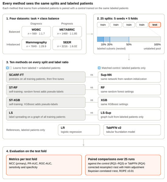
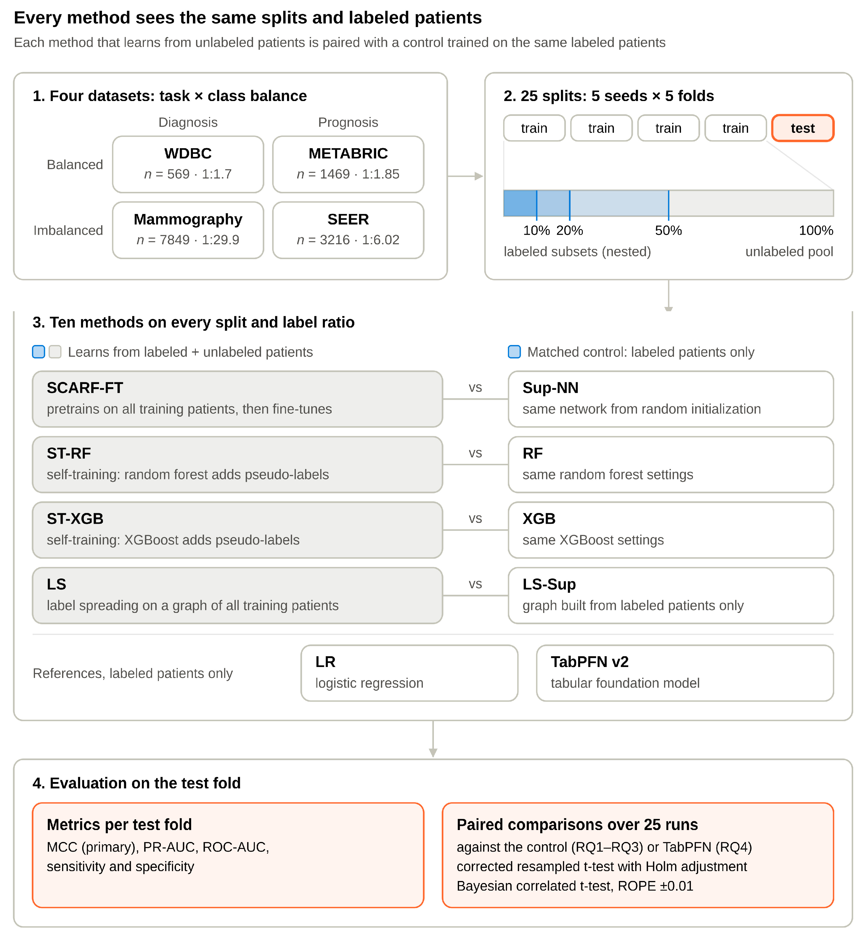
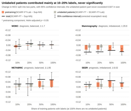
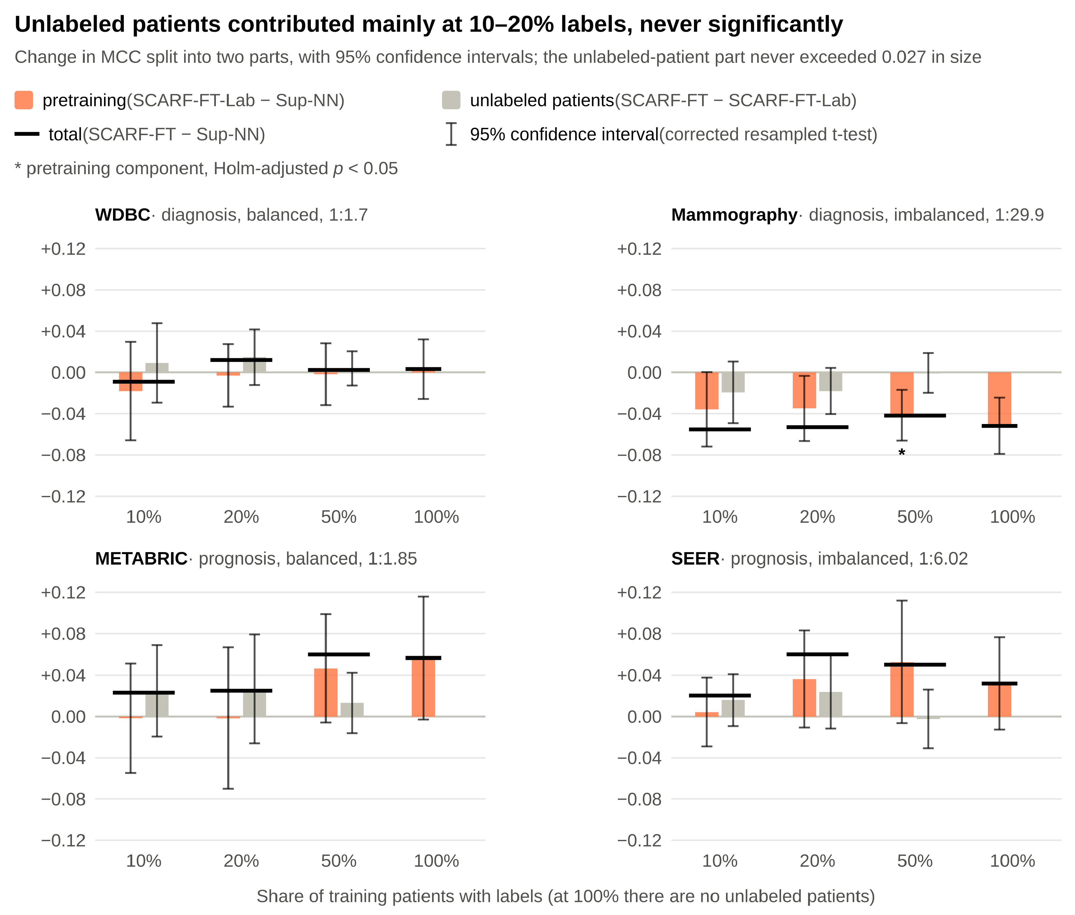
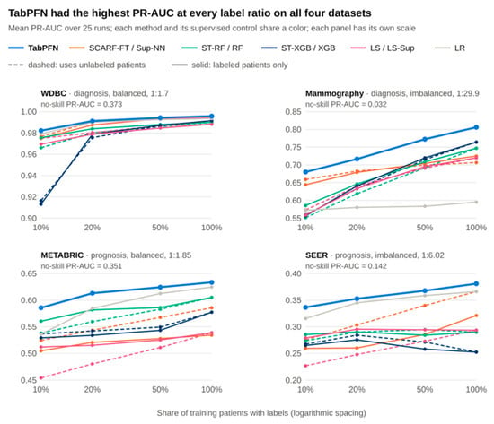
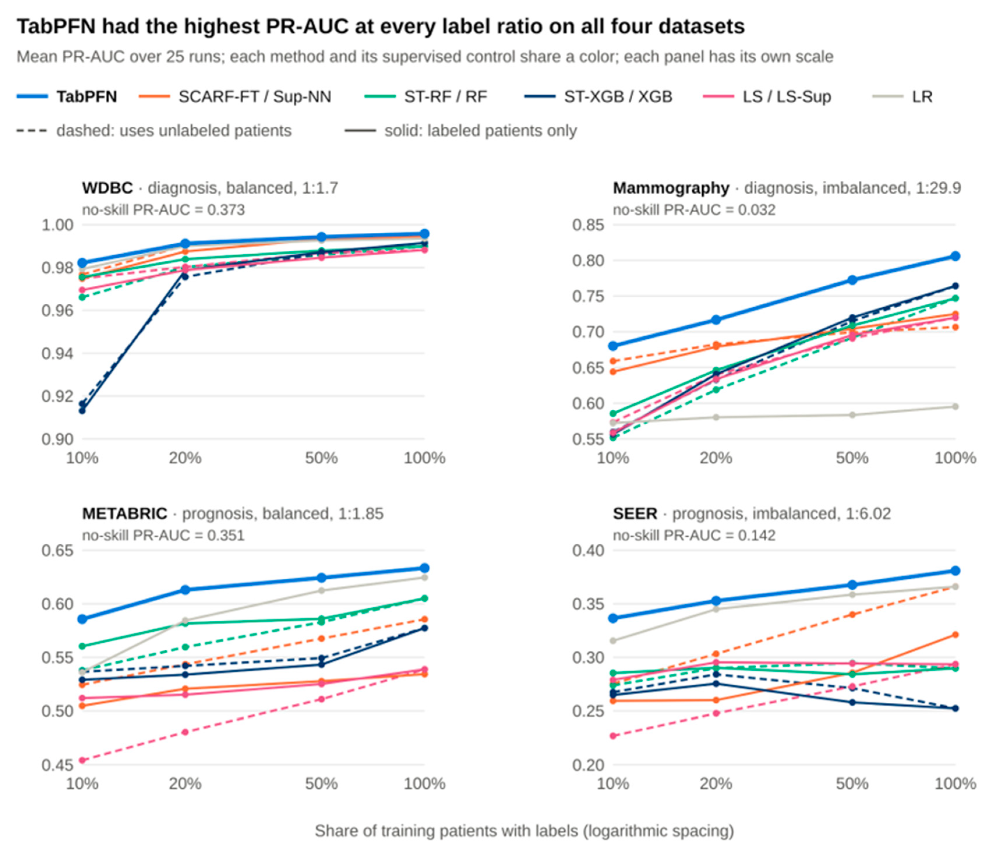

Disclaimer/Publisher’s Note: The statements, opinions and data contained in all publications are solely those of the individual author(s) and contributor(s) and not of MDPI and/or the editor(s). MDPI and/or the editor(s) disclaim responsibility for any injury to people or property resulting from any ideas, methods, instructions or products referred to in the content. |
© 2026 by the authors. Licensee MDPI, Basel, Switzerland. This article is an open access article distributed under the terms and conditions of the Creative Commons Attribution (CC BY) license.