


Simple Summary
Computer programs that recognise cancer in microscope images of oral tissue work well on images like those they were trained on, but they may fail on tissue from another organ. We tested whether such programs could detect breast cancer that has spread to lymph nodes. Every program trained only on oral tissue failed, whatever its design, and neither retraining on oral images nor adjusting to unlabelled lymph node images helped. A different approach worked: we kept a large pathology model unchanged and showed it a small number of labelled lymph node images. With 50 labelled examples of normal tissue and 50 of metastasis, the model separated the two well, close to a model trained on 20,000 labelled images. This suggests that a few dozen labelled examples from the target tissue are a practical way to adapt an existing model to a new setting. The oral images are not needed for this step: the lymph node examples replace the part of the program that was trained on oral tissue.
Abstract
Background/Objectives: Deep networks trained to recognise oral squamous cell carcinoma (OSCC) in histopathology perform well on held-out images from the same collections, but a recent study found that such a network lost most of its discriminative ability on lymph node tissue. We examined whether encoder fine-tuning or label-free adaptation changes this, and how many labelled target patches are needed to recover performance. Methods: The source domain comprised 23,290 images of oral and oropharyngeal mucosa from three public collections. The target domain was PatchCamelyon, a public dataset of sentinel lymph node patches from breast cancer patients; its metastases are breast carcinoma, so the transfer crosses both tissue type and cancer histology. We used 40,000 target patches from 216 slides, split into slide-disjoint adaptation and evaluation pools. We compared nine encoders in ten configurations, including three pathology foundation models (Phikon, Phikon-v2 and the recent Midnight model). We evaluated direct transfer with frozen and fine-tuned encoders, label-free adaptation, and few-shot adaptation, in which we compute class prototypes from k labelled target patches using a frozen encoder. All results are at patch level. Results: Direct transfer failed for every configuration (external AUROC 0.35–0.64), including fine-tuned networks (mean over three seeds 0.44–0.52) and fine-tuned Phikon (0.54–0.58). Label-free methods did not close the gap; a zero-shot vision–language model reached 0.77. With a frozen Phikon encoder, prototypes from 10 and 50 labelled patches per class reached 0.869 ± 0.056 and 0.930 ± 0.015, against 0.82–0.86 at 50 patches for encoders without histology pre-training and 0.977 for a classifier trained on 20,000 labelled patches. Logistic regression on the same patches performed similarly at one and two patches per class and better from five upward (0.955 at 50). Midnight reached 0.922 with prototypes at 50 patches per class, similar to Phikon. The results were similar when support and evaluation patches came from different scanning centres. Conclusions: For the methods and datasets evaluated, no classifier trained on oral tissue transferred to this cross-tissue, cross-cancer target. Our analyses suggest that the change in what the classes contain mattered more than stain or scale, but they do not separate the causal contributions of tissue, cancer histology and acquisition. Frozen pathology foundation models made label-efficient classification on the target domain inexpensive; this replaces the oral-trained classifier and does not use oral images. The findings concern patch-level classification of breast cancer metastases and do not establish clinical performance for OSCC lymph node metastases.
1. Introduction
Oral and oropharyngeal squamous cell carcinomas form the largest group of head and neck malignancies, and cancers of the lip, oral cavity and pharynx account for several hundred thousand new cases worldwide each year [1,2]. Diagnosis rests on the microscopic examination of haematoxylin and eosin (H&E) sections, and the status of the cervical lymph nodes is among the strongest determinants of stage and outcome. Both tasks are time-consuming and subject to inter-observer variation, which has motivated many deep-learning studies of carcinoma recognition in digitised tissue [3,4,5].
Most of these models are developed and tested on images from one source. Performance measured in this way says little about behaviour under distribution shift, and in histopathology shift is common: staining, scanners, magnification, tissue preparation and the tissue itself differ between laboratories and organs [6,7,8,9]. Models may also exploit regularities that are specific to a collection and unrelated to disease [10,11]. Evaluation on independent data therefore decisively tests what a network has learned.
Paun et al. [12] carried out such a test for oral cancer. They used an ImageNet-pre-trained EfficientNet-B0 as a frozen feature extractor with a small classification head, trained on three public collections of oral and oropharyngeal images, and applied it without modification to lymph node patches from PatchCamelyon. Accuracy fell from 91.5% to 56.9% and specificity to 33.3%, while sensitivity stayed at 90.7%, which suggests partial transfer of malignant morphology. Two features of this setting matter for interpretation. First, PatchCamelyon contains sentinel lymph nodes of breast cancer patients, so the experiment changes the tissue (oral mucosa to lymph node) and the cancer (squamous cell carcinoma to breast carcinoma) at the same time. Second, sensitivity and specificity at one threshold cannot distinguish transferred morphology from a decision threshold that has moved; a threshold-free measure is needed.
We revisit this setting with a wider range of encoders, including pathology foundation models pre-trained by self-supervision on histology [13,14,15,16,17,18,19], and ask three questions. Does any encoder transfer directly, frozen or fine-tuned? Can unlabelled target data repair the classifier? If labels are required, how many, and how should they be chosen? To answer the third question we use class prototypes on a frozen encoder [20,21], which require no training and no hyper-parameter search, and compare them with a linear probe on the same labelled patches.
The contributions are mainly experimental. The components of the few-shot method (a frozen foundation encoder, feature standardisation, class prototypes and a cosine classifier) are established techniques [20,21,22]; we do not claim a new learning algorithm. The study adds the following:
- A controlled benchmark of nine encoders in ten configurations under identical data, splits and metrics, covering direct transfer with frozen and fine-tuned encoders, label-free adaptation and few-shot adaptation, with slide-level confidence intervals and paired tests.
- A re-examination of the earlier observation, showing that high sensitivity with low specificity corresponds to near-chance ranking.
- An analysis of the sources of the shift that separates image scale, tissue background and cancer type as far as the public data allow, including a field-of-view control, class-conditional embedding distances and experiments in which only the normal class is labelled, with an unlabelled target pool of varied tumour content.
- A label-efficiency analysis of prototype classification and logistic regression from 1 to 2000 labelled patches per class, with slide-restricted, slide-balanced and diversity-based support sampling, label noise and a cross-centre test, leading to a practical recommendation on when each head should be used. These recommendations are exploratory: the configuration we emphasise was chosen after the results were seen.
2. Related Work
Deep learning for oral cancer histopathology. Public image sets of normal oral epithelium and OSCC [23] have enabled many classifiers that report accuracies above 90% [4,5]. These collections consist of microscope fields captured with a camera, are often redistributed with augmented copies, and lack patient identifiers.
Domain shift in computational pathology. Variation in staining and scanning degrades histology models [6,7]; stain normalisation and stain augmentation are the usual counter-measures [8,24]. Multi-centre challenges show that generalisation across scanners, tumour types and species remains difficult [9]. The CAMELYON datasets of sentinel lymph node sections from breast cancer patients [25,26] and PatchCamelyon [27] are widely used to study these effects.
Pathology foundation models. Self-supervised pre-training of vision transformers [28] on large collections of histology tiles, with objectives such as iBOT [29] and DINOv2 [30], has produced encoders including CTransPath [13], Phikon [14], Phikon-v2 [15], UNI [16], Virchow and Virchow2 [17,31], Prov-GigaPath [18], Hibou [32] and Midnight [19]. Several of the largest models are released under gated licences that require individual approval; Midnight, a ViT-g/14 model trained on 12,000 slides, is openly licensed and is reported to perform similarly to the gated models on public pathology benchmarks [19]. They are usually assessed by linear probing and few-shot classification on frozen embeddings within a target dataset [16,33,34].
Vision–language models. PLIP [35], QuiltNet [36] and CONCH [37] align histology images with text and can classify images from class descriptions without labelled examples.
Few-shot classification on frozen embeddings. Prototypical networks classify a query by its distance to class means computed from a few labelled examples [20]. SimpleShot showed that nearest-centroid classification with centring and L2 normalisation of features from a fixed encoder is a strong baseline [21], and related work found the same for linear classifiers on frozen embeddings [22,38]. The prototype classifier used here is this established protocol.
Unsupervised adaptation. With only unlabelled target data, common strategies align feature statistics, for example by CORAL [39] or by re-estimating batch-normalisation statistics (AdaBN) [40], train domain-invariant features adversarially [41], or adapt at test time [42]. All assume that the relation between features and labels is shared between domains. One-class and anomaly detection methods [43,44,45] learn from normal examples only.
3. Materials and Methods
3.1. Datasets
All data are public. The composition is given in Table 1.
Table 1.
Datasets. SCC: squamous cell carcinoma. Counts for DS1–DS3 are the images used after the exclusion described in the text.
Source domain. DS3 contains, besides normal mucosa and well-, moderately- and poorly-differentiated SCC, 2068 images of oral submucous fibrosis, a potentially malignant disorder that we excluded. The totals are then 14,760 malignant and 8530 normal images, the totals stated in [12]. All three datasets come with predefined training, validation and test folders; DS3 has no validation folder, and 15% of its training images, stratified by grade, were set aside.
Target domain. PatchCamelyon consists of 96 × 96 pixel patches at about 0.97 µm per pixel, down-sampled by a factor of four from 40× scans of sentinel lymph nodes of breast cancer patients in CAMELYON16 [25,26,27]; a patch is positive if its central 32 × 32 pixel region contains tumour. The metastases are breast carcinoma, not OSCC. Using the slide identifiers in the official metadata, we divided the slides of the training partition at random into two halves and drew 20,000 patches from each. The evaluation pool and the adaptation pool share no slides. All target results were computed on the evaluation pool; statistics and labelled examples used for adaptation come only from the adaptation pool. The evaluation pool contains 62 slides without tumour and 46 with tumour, with each tumour-bearing slide contributing at least 109 metastatic patches. Both pools come from the same dataset and acquisition environment, so the evaluation is internal to PatchCamelyon and slide-disjoint, not an external institutional validation. PatchCamelyon slides were scanned at two centres; following the CAMELYON16 documentation [25,26], we assigned slides to Radboud University Medical Center (normal 1–100, tumour 1–70) or University Medical Center Utrecht (the remainder) for the cross-centre analysis in Section 4.6.
Further tissues. As a supplementary check on the separate roles of tissue and cancer type, we used two tasks from the multi-cancer collection that provides DS2: lung SCC against benign lung, which shares the cancer histology of the source but not the tissue, and colon adenocarcinoma against benign colon. These images appear to derive from LC25000 [46], which was built by augmenting 250 original images per class; 1000 images per class from the predefined validation and test folders were used.
Duplicate screening. The source images were screened for near-duplicates with a 64-bit perceptual difference hash (Hamming distance ≤ 6) combined with a cosine similarity of at least 0.90 between Phikon embeddings. Because a hash misses rotated or mirrored copies, we also recorded for every image the highest embedding similarity to any image of another collection. The screening covered every pair of images, so it included pairs between the training and validation folders, between training and test, between validation and test, and pairs across the three collections. Known duplicates were not removed before model selection; the regularisation strength of every oral classifier was chosen on a validation fold that contained near-duplicates of training images. Section 4.2 reports how removing them changes the results.
Pre-training data. DINOv2 was pre-trained on natural images. According to their model cards, Phikon was pre-trained on 40 million tiles from The Cancer Genome Atlas, and Phikon-v2 on about 456 million tiles from TCGA, CPTAC, GTEx and collections of The Cancer Imaging Archive [14,15]. CAMELYON is not named among these sources; we could not inspect the complete list of archive collections.
3.2. Problem Formulation
Let denote nS labelled source images and the target domain, with y ∈ {0,1} for normal and malignant tissue. An encoder with weights θ maps an image x to an embedding of dimension d, and a head with parameters ϕ returns the probability of malignancy. We study regimes that differ in the target information available: direct transfer, in which θ and ϕ are determined from alone; unsupervised adaptation, with an unlabelled target sample ; normal-only labels, with k target patches known to be normal; few-shot adaptation, with a support set of k labelled target patches per class; and a target-supervised reference, in which all N = 20,000 adaptation patches are labelled.
Two kinds of difference separate the domains. The marginal distributions differ, PS(x) ≠ PT(x), because of staining, acquisition and scale. The class-conditional distributions P(x∣y) differ as well, for two separate reasons: the normal class changes from stratified squamous mucosa to lymphoid tissue (tissue shift), and the malignant class changes from squamous cell carcinoma to metastatic breast carcinoma (cancer-histology shift).
3.3. Encoders
Table 2 lists the nine encoders; we used EfficientNet-B0 at two input sizes, yielding ten configurations. Midnight [19] was run through every analysis of the main comparison with the same code. All were used with their published weights; the exact model revisions are listed in Supplementary Table S13. Images were resized to the input size of each encoder (bicubic interpolation, antialiased when down-scaling) and normalised with the statistics of the corresponding pre-training. Oral images were first reduced to 256 pixels on the short side and centre-cropped. The embedding fθ(x) is the class token after the final layer normalisation for the vision transformers (DINOv2, Phikon, Phikon-v2), the class token concatenated with the mean of the patch tokens for Midnight, as recommended by its authors (3072 dimensions, input normalised with mean and standard deviation 0.5) and the globally average-pooled feature map of the last stage for EfficientNet, ConvNeXt V2, Swin V2 and MambaVision.
Table 2.
Encoders. d: embedding dimension.
3.4. Proposed Method: Few-Shot Prototype Adaptation of a Frozen Foundation Encoder
3.4.1. Pipeline Overview
The method uses the encoder exactly as released and replaces the source-trained head with a rule defined on the target domain (Figure 1). Three sets of lymph node patches pass through the same frozen encoder: an unlabelled adaptation pool, a support set of k labelled patches per class and the query patches to be classified. The pool supplies the statistics used to standardise every embedding, the support set supplies one prototype per class, and each query is assigned to the closest prototype. No weight is updated at any stage. The baseline, shown at the bottom of Figure 1, keeps the same encoder but uses a linear head trained on the oral images only.
Figure 1.
Proposed pipeline. A frozen pathology foundation encoder embeds an unlabelled target pool, a support set of k labelled patches per class and the query patch; embeddings are standardised with the pool statistics, class prototypes are formed from the support set, and the query is classified by cosine similarity. Bottom: the direct-transfer baseline and its external AUROC on PatchCamelyon (breast cancer metastases).
3.4.2. Model Architecture and Classification Rule
Figure 2 shows the two components of the model in detail. The encoder (Figure 2A) is a Vision Transformer that turns each patch into a 768-dimensional class-token embedding fθ(x); it is run once per patch and never fine-tuned. The classifier (Figure 2B) follows the SimpleShot protocol [21] and has three steps.
Figure 2.
Architecture of the proposed model. (A) Frozen encoder (Phikon, ViT-B/16): resizing and patch partition, patch embedding with class token and position embedding, one of the 12 Transformer blocks expanded (multi-head self-attention and MLP, each with a residual connection), and the class-token attention of the last block for the example patch. (B) Prototype classifier: encoding and standardisation with the statistics of the unlabelled pool, prototypes c0 and c1 from k = 50 labelled patches per class, cosine similarities s0 and s1, and the probability p. (C) The classifier in the embedding space (UMAP of 3000 evaluation patches with the two prototypes and the query) and the distribution of s1 − s0 over all 20,000 evaluation patches. All images, values and distributions are computed by the model. Arrows indicate the flow of data between processing steps.
Target standardisation. Embeddings are centred and scaled per dimension with the mean μT and standard deviation σT of the unlabelled adaptation pool of N patches,
where the division and the square are taken element-wise.
Class prototypes. From the support set, one prototype per class is formed as the normalised mean of the standardised embeddings [20],
where k is the number of labelled patches per class.
Cosine classifier. A query patch x is scored by its cosine similarity sy(x) to each prototype, and the difference is mapped to a probability p(x) with a fixed temperature τ,
The positive class is assigned when p(x) ≥ 0.5, that is, when the query is closer to the metastasis prototype. We set τ = 10 before any evaluation and did not tune it on the evaluation pool; because τ rescales a monotone function, it changes calibration but not ranking or decisions (Section 4.8). Figure 2B traces these steps for one evaluation patch, and Figure 2C shows the resulting decision in the embedding space and the distribution of s1 − s0 over the evaluation pool.
3.4.3. Choice of Classification Head
We present the prototype classifier as the proposed method, although a linear probe on the same frozen embeddings is more accurate once five or more labelled patches per class are available and is not worse with one or two (Section 4.7), for three practical reasons. It has no trainable parameters and no hyper-parameters to select, so there is nothing to over-fit or tune on a handful of examples. Under the random label flipping we tested, its AUROC decreased less than that of logistic regression with the fixed regularisation we used (Section 4.7). And it is the standard few-shot protocol for pathology foundation models [16,21], which makes results comparable across studies. Section 5 gives a recommendation for choosing between the two heads.
3.5. Comparators
Direct transfer with a frozen encoder. Following [12], a head was trained on source embeddings and applied unchanged to the target. We used -regularised logistic regression on standardised embeddings zi with labels ,
with weight vector w, bias b and class weights ωy inversely proportional to class frequency. The regularisation parameter C ∈ {10−3,10−2,10−1,1,10} was selected by AUROC on the source validation fold; the problem is convex, so results do not depend on a seed.
Direct transfer with end-to-end fine-tuning. EfficientNet-B0, Swin V2-Tiny and MambaVision-Tiny (three seeds each) and Phikon (one seed) were fine-tuned on the source training fold with a linear head and class-weighted binary cross-entropy, for at most six epochs with early stopping on validation AUROC (patience two), using AdamW (learning rate 5 × 10⁻⁵ for the encoder and 10−3 for the head, weight decay 0.05), one epoch of warm-up followed by cosine decay, mixed precision and gradient clipping at unit norm. Augmentation consisted of random resized crops (scale 0.6–1), flips and rotations by multiples of 90°. Each model was trained with and without H&E stain augmentation [8]: after colour deconvolution with the Ruifrok–Johnston matrix M [52], with optical density o = −logx, each stain channel c is perturbed independently,
and the image is recovered as .
Label-free adaptation. (i) Standardising target embeddings with target instead of source statistics; (ii) CORAL [39], which whitens target embeddings with the target covariance and re-colours them with the source covariance and mean μS,
The remaining methods were (iii) self-training for three rounds on the 20% most confidently positive and negative pseudo-labelled adaptation patches; (iv) AdaBN [40] on the fine-tuned networks with batch normalisation (EfficientNet-B0 and MambaVision, all seeds); and (v) zero-shot classification with the vision–language model PLIP [35], using five pairs of text descriptions of normal lymph node and metastasis (Supplementary Table S12).
Few-shot comparators. On the same support sets as the prototype classifier: logistic regression (Equation (4) with C = 10−2 and equal class weights), a Euclidean nearest-centroid rule, prototypes with several centroids per class, and the source classifier refitted on source data together with the support set. The target-supervised reference is logistic regression on all 20,000 labelled adaptation patches, with C chosen by five-fold cross-validation on the adaptation pool, grouping the folds by slide, so that the reference uses target data only. Taking C from the oral validation fold for the reference (C = 1 for Phikon) gives an AUROC of 0.968, whereas the value used for the large-support curve, C = 10−2, gives 0.976; the two values therefore differ in regularisation, not in data or preprocessing. With the target-only choice (C = 10−3 for Phikon) the reference reaches 0.977, and every comparison with the reference, including Equation (9), uses this single definition.
3.6. Analysis of the Sources of Shift
Field of view. A PatchCamelyon patch covers about 93 µm of tissue, an oral microscope field several times more. We re-cropped every oral image at original resolution to the central one-half, one-quarter and one-eighth of its shorter side and repeated direct transfer for EfficientNet-B0, Phikon and Phikon-v2, with all collections and with DS3 alone (400× fields, where the crop fraction has a single physical meaning).
Class-conditional embedding distances. For four encoders, the squared maximum mean discrepancy (MMD) with a Gaussian kernel (median bandwidth) was computed between oral normal, oral SCC, lymph node normal and lymph node metastasis, on a common standardisation of source and target embeddings.
Normal-only labels. With k normal target patches and no labelled tumour, we tested a centroid rule −s0(x) that uses the unlabelled pool for standardisation, a one-class detector using the normal patches alone (standardised distance from their mean) [43,44], and a classifier separating oral carcinoma from the target normals. These separate the change of the normal background from the change of cancer type. Because the centroid rule depends on the unlabelled pool through the standardisation, we repeated it with pools of 9000 adaptation patches containing 0%, 1%, 10%, 25% or 50% tumour, keeping the pool size, the 20 draws of 50 labelled normal patches and the evaluation pool fixed. All pool patches came from the adaptation partition, and each condition used a new random pool for every draw.
Location of false positives. The fraction of normal lymph node patches called malignant by direct transfer was computed by tertile of a nuclear-density proxy (fraction of pixels with luminance below 110, and mean haematoxylin optical density).
Lung and colon. Direct transfer to lung SCC, which keeps the cancer histology of the source while changing the tissue, was compared with transfer to colon adenocarcinoma.
3.7. Support-Set Sampling and Robustness
Support sets were drawn at random, 20 times for each k ∈ {1,2,5,10,20,50,100} (ten times for k ≥ 200), from the 108 adaptation slides, and we report how many distinct slides they contain. We compared random sampling with (i) slide-balanced sampling, which takes one patch from each slide in turn so that as many slides as possible are represented; (ii) diversity-based selection, which is label-agnostic and could be applied before annotation: k-means with 2k clusters on the unlabelled pool, after which the patch nearest each cluster centre is labelled; and (iii) slide-restricted sampling, in which normal and metastatic support patches come from the same one, two or five tumour-bearing slides. We also flipped 10–50% of the support labels, chosen at random across both classes, and in a cross-centre test drew support patches from one scanning centre and evaluated on each centre separately. By default, the standardisation statistics for the cross-centre test come from the whole adaptation pool, which contains slides of both centres (12,082 Radboud and 7918 Utrecht patches). We also report a stricter variant in which the statistics come only from the adaptation patches of the centre that supplies the support set.
3.8. Evaluation and Statistics
Source splits. We report the random 60/20/20 split of [12] (five seeds; Supplementary Table S2), the predefined folders of each collection (native split: 19,101 training, 2206 validation and 1983 test images), which is the headline protocol, and leave-one-dataset-out.
Metrics. We report accuracy, sensitivity, specificity, precision, F1-score, balanced accuracy and the Matthews correlation coefficient [53],
where TP, TN, FP and FN are the counts of true and false positives and negatives. We also report the fraction of positive calls, AUROC, the area under the precision–recall curve (AUPRC), sensitivity at fixed specificities of 90%, 95% and 98%, the Brier score, and the expected calibration error [54] over B = 15 equal-width bins Ib of n predictions,
where acc(Ib) is the fraction of positives and conf(Ib) the mean predicted probability in bin b. For direct transfer, thresholds were fixed without target data: 0.5, and the Youden-optimal threshold [55] on the source validation fold. The fraction of the achievable improvement obtained with k patches per class is given relative to chance,
where AUROCsup is the target-supervised reference.
Uncertainty. Two sources of variation are reported separately. Variation due to the choice of support patches is the standard deviation over support draws. Variation due to the finite evaluation set is estimated by a percentile bootstrap of 1000 resamples in which whole slides, not patches, are resampled. Differences between methods were tested in a paired design: for the same ten support draws, the AUROC difference was averaged over draws within each of 500 slide-level bootstrap resamples, giving a 95% interval and a two-sided p-value. The slide-bootstrap intervals are conditional on the support draws used; the variability across draws is the standard deviation given separately. The p-values of the 23 paired comparisons in Section 4.5 and Section 4.7 were adjusted using the Holm procedure; with 500 resamples, the smallest attainable unadjusted p-value is 0.002. Displayed single runs are the draws with the median AUROC among 20. The configuration emphasised in the text (Phikon with k = 50) was chosen after inspecting the results, and its interval does not account for that choice; recommendations derived from it should be read as exploratory. Sensitivity at fixed specificity is reported in two ways: retrospectively, from the ROC curve of the evaluation pool, and prospectively, with the threshold set on a separate calibration set of 250 labelled normal adaptation patches that were not in the support set and then applied unchanged to the evaluation pool.
Implementation. Python 3.12 (Python Software Foundation, Wilmington, DE, USA), PyTorch 2.5 [56] (PyTorch Foundation, San Francisco, CA, USA), timm 1.0 (Hugging Face, New York, NY, USA) and scikit-learn 1.9 [57] (open-source software, scikit-learn developers) on one NVIDIA GeForce RTX 3060 GPU (12 GB; NVIDIA Corporation, Santa Clara, CA, USA). The selective-scan operator of MambaVision is normally a compiled kernel; we used an implementation of the same recurrence in PyTorch, which reproduced a direct step-by-step evaluation of the recurrence exactly (maximum absolute difference 0 in single precision) on random inputs. Embeddings were extracted once and cached. The code, configuration files, exact model revisions (Supplementary Table S13), preprocessing settings, slide identifiers of both pools, all support-set indices and seeds, classifier settings and per-patch predictions are available at https://github.com/sumon39cst/oral-to-lymph-node-fewshot (version tag revision-2; accessed on 4 November 2026).
4. Results
4.1. Direct Transfer Fails for Every Encoder
Results for frozen encoders under the native split are given in Table 3 and Figure 3, and all metrics for every configuration, split and threshold in Supplementary Table S1. On oral tissue the ImageNet-based encoders performed similarly (accuracy 0.88–0.91, AUROC 0.95–0.97), and the pathology foundation models were better (accuracy 0.96, AUROC 0.99). On breast cancer lymph node metastases, no configuration was usable (AUROC 0.353–0.644). Midnight, which is not included in Table 3 or Figure 3 (see Supplementary Table S23), behaved the same way: internal AUROC 0.998 and external AUROC 0.412. For five of the nine configurations in Table 3 the upper confidence limit was below 0.5, meaning that the scores were systematically ordered against the labels.
Table 3.
Direct transfer with frozen encoders (native split, threshold 0.5). Internal: oral test folds (n = 1983). External: PatchCamelyon evaluation pool (n = 20,000, breast cancer metastases). Brackets: 95% slide-cluster bootstrap interval. The table covers the nine configurations of the original comparison; Midnight is reported in the text.
Figure 3.
Direct transfer with frozen encoders. Pale bars: internal oral test; solid bars: PatchCamelyon evaluation pool (breast cancer metastases). Error bars: 95% bootstrap intervals (slide-cluster for the external test). Nine configurations of the original comparison; Midnight is reported in the text.
The row for EfficientNet-B0 at 96 pixels reproduces the qualitative pattern of [12] (their accuracy 0.569, sensitivity 0.907, specificity 0.333): accuracy 0.545, sensitivity 0.893, specificity 0.192. The samples of PatchCamelyon and their prevalence differ between the studies, so the agreement is in kind and not in value. The associated AUROC is 0.586, and 85% of all patches are called positive; the high sensitivity results from the position of the threshold on the new tissue.
4.2. Source Collections: Duplicates and Leakage
The screening found 186 near-duplicate pairs between DS1 and DS2 (283 images) and none involving DS3 (Supplementary Table S8). In embedding space, the most similar DS1 image for a DS2 image had a median cosine similarity of 0.92, against 0.48–0.53 between DS3 and the other two collections, so the oral subset of DS2 very probably derives from the same original images as DS1, partly as augmented copies. Within collections, a near-duplicate in the training folder was found for 6 of 246 validation and test images in DS1, 46 of 2002 in DS2, and 157 of 1941 in DS3; augmented versions of the same original therefore occur on both sides of the predefined folders. Removing the 127 test images with a near-duplicate in training or validation changed no internal AUROC by more than 0.001 and no accuracy by more than 0.002 (Supplementary Table S10); no image was excluded from the main analysis. To see whether the duplicates affect the main external result, we also refitted every oral classifier after removing all near-duplicates: the 1705 images in 749 connected groups of near-duplicate pairs (within and across collections, and between training, validation and test) were reduced to one image per group, keeping a training image where possible, so 956 images were removed; the regularisation strength was again chosen on the cleaned validation fold. Internal AUROC changed by −0.001 to 0.000 and external AUROC by at most 0.011, and direct transfer still failed for every encoder (external AUROC 0.359–0.643; Supplementary Table S17). The duplicates therefore inflate the internal results slightly but do not explain the failure on lymph node tissue. Because patient identifiers are unavailable, patient-level leakage cannot be excluded, and internal results should be read as optimistic.
Generalisation between oral collections was limited (Table 4). With DS3, the only collection independent of the others, held out, AUROC was 0.34–0.72; training on DS3 and testing on DS1 and DS2 together gave 0.49–0.65. The failure on lymph node tissue is the far end of a problem that already exists between oral collections.
Table 4.
Generalisation between oral collections (frozen encoders, AUROC on the held-out data). DS1 and DS2 share source images; DS3 is independent. Nine configurations of the original comparison; Midnight was not included.
4.3. Fine-Tuning and Label-Free Adaptation
Fine-tuning raised internal accuracy to 0.974–0.991 but left external performance at chance (Table 5; Supplementary Figure S2). Over three seeds the mean external AUROC of the three ImageNet architectures was 0.44–0.52, and stain augmentation changed it by at most 0.023, less than the standard deviation between seeds (up to 0.058). Fine-tuned Phikon reached 0.544 without and 0.584 with stain augmentation.
Table 5.
End-to-end fine-tuning (native split, threshold 0.5). ImageNet architectures: mean ± SD over three seeds. Phikon: one seed, 95% slide-cluster interval.
Label-free methods were also ineffective (Table 6). Target standardisation, CORAL and self-training left the AUROC between 0.31 and 0.62. AdaBN lowered the AUROC of the fine-tuned networks to 0.42–0.44 (mean over seeds; Supplementary Table S9). Zero-shot PLIP, which is told in words what the classes are, reached 0.772 (95% CI 0.732–0.813), the best label-free result, with single prompt pairs ranging from 0.631 to 0.807. Adversarial adaptation and entropy-based test-time adaptation were not evaluated. For Midnight, target standardisation, CORAL and self-training gave 0.433, 0.582 and 0.399.
Table 6.
External AUROC (PatchCamelyon) along the target-information ladder. Few-shot columns: prototype classifier, mean over 20 draws. Reference: logistic regression on 20,000 labelled adaptation patches, regularisation chosen by slide-grouped cross-validation on the adaptation pool.
4.4. Sources of the Shift
Scale. Re-cropping the oral images did not restore transfer at any field of view (Table 7; Figure 4c). External AUROC varied between crop sizes by more than the slide-level intervals (about ±0.05), but without any trend, and at one quarter of the field, the size closest to the target patches, every encoder was at or below chance. Restricting the source to the 400× collection gave 0.38–0.55 (EfficientNet-B0), 0.28–0.43 (Phikon) and 0.52–0.62 (Phikon-v2), with internal AUROC of at least 0.93. Harmonising the field of view therefore does not remove the failure; sharpness, which also differs, could not be matched.
Table 7.
Field-of-view control: AUROC of direct transfer on PatchCamelyon after re-cropping the oral training images, with 95% slide-cluster intervals.
Figure 4.
Sources of the shift. (a) External AUROC when only normal lymph node patches are labelled (with the unlabelled pool), compared with direct transfer and with both classes labelled; one row for each of the nine configurations of the original comparison (Midnight not included), markers for the amount of target information. (b) Fraction of normal lymph node patches called malignant by direct transfer, by tertile of nuclear density. (c) Field-of-view control with 95% slide-cluster intervals (solid: external; dashed: internal). Dotted horizontal lines in (a,c): chance.
Class-conditional embedding distances. The four classes were far apart across domains and close within each domain (Table 8). For all four encoders tested, the MMD between oral and lymph node classes (0.12–0.30) was two to ten times the MMD between normal and metastatic lymph node tissue (0.03–0.07). Oral SCC was not closer to lymph node metastasis than to normal lymph node tissue for EfficientNet-B0 or DINOv2 (MMD 0.146 against 0.122, and 0.141 against 0.126), and for Phikon oral normal mucosa was closer to lymph node metastasis (0.266) than to normal lymph node tissue (0.297). A classifier trained on oral tissue cannot be expected to handle this class-conditional arrangement.
Table 8.
Squared maximum mean discrepancy between class-conditional embedding distributions (common standardisation; larger values mean further apart).
Normal background and cancer type. Labelling target normals while keeping the unlabelled pool restored most of the performance without any tumour label (Figure 4a): with Phikon, 0.911 with 50 normal patches and 0.931 with 1000. This result, however, depends on the unlabelled pool, which was about half metastatic. With pools of the same size (9000 patches) and the same 50 labelled normals, AUROC was 0.910 ± 0.028 with 50% tumour, 0.857 with 25%, 0.730 ± 0.088 with 10%, 0.569 with 1%, and 0.551 with none (Figure 5; Supplementary Table S20). Lowering the tumour proportion from 50% to 10% reduced the AUROC in all 20 draws by 0.181 on average (range 0.088 to 0.323). The rule works because standardisation with a mixed pool places the normal prototype away from the pool centre in a direction that separates the classes; when tumour is rare, that direction no longer carries information about metastasis. Using the statistics of the 50 normals alone, without any pool, gave 0.797. The two-class prototype classifier was far less sensitive to the pool (0.930 with 50% and 0.903 with 10% tumour, 0.871 with none). The normal-only result is thus specific to a tumour-rich unlabelled pool and should not be expected where metastatic tissue is rare. Normal patches used strictly alone, as a one-class detector, gave 0.80 with Phikon, 0.72 with Phikon-v2 and 0.43–0.58 with the other seven configurations of the original comparison (0.77 with Midnight). Training oral carcinoma against target normals gave 0.83 and 0.85 for the two pathology models and 0.64–0.81 for the other seven configurations (Midnight was not included in this analysis), below the rule that uses no tumour example at all. Replacing the normal background thus recovers most of the performance when the unlabelled pool is rich in tumour, whereas the oral tumour class does not help to recognise breast carcinoma metastases. On lung, where the cancer histology matches the source, but the tissue does not, direct transfer failed as badly as on lymph node (AUROC 0.07–0.24 for six configurations; Supplementary Table S6), which suggests that a change of tissue alone can be enough to break transfer.
Figure 5.
Dependence on the composition of the unlabelled pool (Phikon, 50 labelled patches per class or 50 labelled normal patches; pools of 9000 adaptation patches with 0–50% tumour; mean ± SD over 20 draws). Grey dashed line: the 50 normal patches used without any pool (one-class). Dotted line: chance.
False positives. Under direct transfer the fraction of normal lymph node patches called malignant rose with nuclear density for eight of the nine configurations of the original comparison (Figure 4b; Supplementary Table S5; Midnight was not included in this analysis; for Phikon 0.23, 0.66 and 0.98 across tertiles), with the same pattern for both density proxies.
4.5. Few-Shot Adaptation
With labelled patches of both classes, every configuration improved steadily with k (Table 6; Figure 6), and the pathology foundation models separated from the rest. At k = 10 the prototype classifier reached 0.869 with Phikon and 0.832 with Phikon-v2, against 0.733–0.784 for the seven other configurations of the original comparison; at k = 50 it reached 0.930 and 0.919, against 0.818–0.857. In paired tests Phikon exceeded each of the seven other configurations by 0.077–0.118 at k = 50 (all Holm-adjusted p = 0.046, the smallest value attainable with 500 resamples and 23 tests; Supplementary Table S7); Phikon and Phikon-v2 did not differ at k = 50 (0.009, 95% CI −0.002 to 0.020; Holm-adjusted p = 0.232). Relative to chance, Phikon recovered 77% of the achievable improvement at k = 10 and 90% at k = 50 (relative to the target-supervised reference AUROC of 0.977). Midnight, the largest and most recent model in the comparison, reached 0.898 ± 0.030 at k = 10 and 0.922 ± 0.019 at k = 50; the paired difference from Phikon was +0.021 (95% CI −0.004 to 0.045) and −0.007 (−0.028 to 0.013), so the newer model did not change the label-efficiency curve in this task. With logistic regression Midnight reached 0.955 at k = 50 (paired difference from Phikon +0.001, −0.011 to 0.011). The Midnight comparisons are not part of the Holm family of 23 comparisons; they are reported with unadjusted 95% intervals.
Figure 6.
Prototype classifier on PatchCamelyon as a function of the number of labelled patches per class: AUROC, balanced accuracy, sensitivity and specificity. Lines: mean over 20 draws; bands: ±one standard deviation. Dotted lines: direct transfer and the target-supervised reference for Phikon.
Table 9 gives all metrics for Phikon, and Supplementary Table S3 gives every individual draw. The spread between support draws (standard deviation of AUROC 0.085 at k = 5, 0.015 at k = 50) was larger than the uncertainty due to the evaluation slides for k ≤ 20 (0.014–0.033) and similar at k = 50 (0.017). For the median draw at k = 50, 8390 of 10,067 metastatic and 8929 of 9933 normal patches were classified correctly: accuracy 0.866 (95% CI 0.828–0.896), sensitivity 0.833 (0.756–0.894), specificity 0.899 (0.876–0.922) and AUROC 0.935 (0.907–0.957). Receiver operating characteristic and precision–recall curves are shown in Figure 7 and confusion matrices in Figure 8; both show the median draw, which at k = 10 (AUROC 0.897) lies above the mean over draws (0.869).
Table 9.
Prototype classifier on frozen Phikon embeddings, PatchCamelyon evaluation pool: mean ± SD over 20 support draws for every metric.
Figure 7.
ROC curves (left) and precision–recall curves (right) on the PatchCamelyon evaluation pool (Phikon encoder) for direct transfer, the prototype classifier at k = 10, 50 and 100 labelled patches per class (median draw) and the reference trained on all 20,000 labels. Values in the legends are AUROC (left) and AUPRC (average precision; right); 95% slide-bootstrap intervals are given in the text. Dotted lines: chance (left) and the prevalence of metastasis (right).
Figure 8.
Confusion matrices on PatchCamelyon for (a) direct transfer and the prototype classifier at (b) k = 10, (c) k = 50 and (d) k = 100 (Phikon; median draw). Cells give the row-normalised percentage and, in parentheses, the number of patches.
4.6. Support-Set Composition and Cross-Centre Evaluation
Random support sets spread over many slides: on average 17.6 distinct slides at k = 10 and 59.6 at k = 50 (Supplementary Table S14). Labelling 50 patches per class is therefore not equivalent to examining 50 slides, but it is far from a single slide. The sampling scheme mattered at small k (Table 10). With five patches per class, label-agnostic diversity-based selection raised the AUROC of the prototype classifier from 0.830 to 0.877 and halved the spread between draws (0.085 to 0.046); slide-balanced sampling gave 0.866. At k = 50 the schemes differed by at most 0.011. Drawing all support patches from a single tumour-bearing slide lowered the AUROC at k = 50, from 0.930 to 0.872 (prototypes) and from 0.955 to 0.891 (logistic regression); with five slides the values were 0.892 and 0.935 (Figure 9a).
Table 10.
Effect of how support patches are chosen (Phikon, mean ± SD of AUROC over 20 draws). Diversity-based selection is label-agnostic, so the class balance of the labelled set varies.
Figure 9.
Robustness of few-shot classification (Phikon). (a) Support patches from one, two or five slides instead of all 108. (b) Label noise in the support set at k = 50, 0–50% of labels flipped at random; the top axis gives the effective number of correctly labelled patches per class, k(1 − 2ρ)2. (c) Large support sets, up to all adaptation patches (ten draws per point). Error bars: SD over draws.
In the cross-centre test, support patches from one scanning centre gave the same performance on patches from the other centre as on their own: with Phikon at k = 50, prototypes reached 0.943 and 0.946 on Radboud and Utrecht patches when the support came from Radboud, and 0.937 and 0.942 with support from Utrecht (Supplementary Table S15). These values used standardisation statistics from the whole adaptation pool, which includes both centres. With statistics from the support centre only, the results were unchanged: 0.944 and 0.949 with Radboud support, 0.935 and 0.943 with Utrecht support (Supplementary Table S18). Both centres belong to the same study and protocol, so this is not an independent institutional validation.
4.7. Prototype Classifier and Logistic Regression
At one and two labelled patches per class the two heads performed almost identically (Table 11; Supplementary Table S21): 0.671 ± 0.094 against 0.675 ± 0.093 at k = 1 and 0.762 ± 0.081 against 0.765 ± 0.089 at k = 2, with paired differences of 0.003 (95% CI 0.001 to 0.005) and 0.002 (−0.001 to 0.005) in favour of logistic regression. From five patches per class onwards logistic regression on the same support sets was better than the prototype classifier (Figure 10; Supplementary Table S11 for all configurations). The paired difference was small at k = 5 (0.016, 95% CI 0.013–0.019) and larger from k = 10 (0.032) to k = 100 (0.044); all differences from k = 5 onwards remained significant after Holm adjustment over the 23 paired comparisons (p = 0.046), and the difference at k = 2 did not (p = 0.268). The prototype classifier levelled off: 0.930 at k = 50, 0.922 at k = 100, 0.932 at k = 200 and 0.934 with all 20,000 adaptation patches, whereas logistic regression rose to 0.976 (Figure 9c). The dip between k = 50 and k = 100 is smaller than the spread between draws and is not a real decline. A single mean per class cannot represent the several tissue patterns within each class, and it weights every embedding dimension equally; using several centroids per class raised the plateau only slightly (0.943 with eight centroids at k = 2000; Supplementary Table S16), so the advantage of logistic regression lies mainly in learning which dimensions discriminate. Cosine and Euclidean prototypes were equivalent, target standardisation made no measurable difference (0.930 against 0.931 without it, at k = 50), and adding the source images to the support set did not help.
Table 11.
Prototype classifier against logistic regression on identical support sets (Phikon, AUROC, mean ± SD over 20 draws; paired difference logistic regression minus prototypes over ten draws with 95% slide-cluster interval; Holm adjustment over 23 comparisons).
Figure 10.
Ablation with Phikon. (Left): standardisation. (Centre): classifier head (the Euclidean curve, dashed, coincides with the cosine curve). (Right): encoder, with the same prototype classifier for the nine configurations of the original comparison (Midnight was not included; thick lines: pathology foundation models).
The prototype classifier was the more robust head when labels were noisy: with 30% of the support labels flipped at k = 50, its AUROC was 0.856, against 0.789 for logistic regression (Figure 9b; Supplementary Table S22); this holds for random label flipping with τ = 10 and C = 10−2, and we did not test systematic errors such as consistent confusion of particular tissue types. Both heads deteriorated sharply between 30% and 40% flipped labels (0.856 to 0.708 for prototypes, 0.789 to 0.649 for logistic regression) and reached chance at 50%. This follows from how random flips act on class means. If a fraction ρ of the support labels is flipped at random, each labelled class becomes a mixture of both true classes, and the expected difference between the two class means, which defines the decision direction of the prototype classifier, shrinks by the factor 1 − 2ρ: 0.8 at 10%, 0.4 at 30% and 0.2 at 40% (observed 0.80, 0.40 and 0.20). The sampling error of the class means does not shrink, so the estimate behaves like a clean support set of about k(1 − 2ρ)2 patches per class: 18 at 20%, 8 at 30% and only 2 at 40%. Consistent with this, the direction estimated from 50 noisy patches per class at 40% noise had a cosine similarity of 0.32 with the direction obtained from all 20,000 labelled adaptation patches, close to that of clean supports with one or two patches per class (0.32 and 0.41), and its AUROC (0.708) was close to that of clean supports at k = 1–2 (0.671–0.762). The collapse at 40% is therefore not a failure of the method but the point at which so few effectively correct labels remain that the classes can no longer be separated. Both heads are computationally negligible: for 100 labelled patches and 20,000 queries, prediction took about 40 ms with prototypes and 11 ms with logistic regression on a CPU, once embeddings were available.
4.8. Operating Points, Calibration and Slide-Level Behaviour
At fixed specificity the prototype classifier (k = 50, median draw) reached a sensitivity of 0.831 (95% CI 0.761–0.892) at 90% specificity, 0.736 (0.651–0.817) at 95% and 0.589 (0.496–0.688) at 98%; logistic regression on the same support set reached 0.881, 0.806 and 0.711 (Table 12). These are retrospective summaries of the ROC curve, because each threshold was read from the evaluation pool itself. With thresholds set prospectively on a separate calibration set of 250 labelled normal adaptation patches, the prototype classifier reached sensitivities of 0.833, 0.769 and 0.671 at realised specificities of 0.888, 0.933 and 0.966 (mean over 20 draws; logistic regression 0.887, 0.845 and 0.779; Supplementary Table S19). At the 0.5 threshold, about one metastatic patch in six was missed. Typical decisions are shown in Figure 11: false negatives were often patches in which a small tumour focus lay among lymphocytes, and false positives included dense fibrous stroma and crowded lymphoid tissue. PatchCamelyon provides no annotation of focus size, so performance for small metastases could not be reported separately; sensitivity did not differ between tertiles of slide-level tumour burden (median 0.905, 0.876 and 0.944). In the embedding space the classes overlap partly, and errors concentrate along their boundary (Figure 12).
Table 12.
Sensitivity at fixed specificity on PatchCamelyon (Phikon, k = 50, median draw; 95% slide-cluster intervals; retrospective: thresholds read from the evaluation ROC curve).
Figure 11.
Predictions of the prototype classifier (Phikon, k = 50, median draw) on patches from unseen slides, with the predicted probability of metastasis. The dashed square marks the central 32 × 32-pixel region; a patch is labelled metastatic only if tumour lies inside it, so tumour outside the square does not make a patch positive.
Figure 12.
UMAP projection [58] of Phikon embeddings of 3000 evaluation patches, coloured by reference label, predicted probability and classification errors. Stars mark the two class prototypes.
The temperature was fixed at τ = 10 before evaluation. Calibration depends on it: the expected calibration error at k = 50 was 0.180, 0.043, 0.061, 0.100 and 0.124 for τ = 2, 5, 10, 20 and 50. Fitting τ on the support set by leave-one-out, without the evaluation set, gave a mean τ of 5.6 and an error of 0.042 (Supplementary Figure S1).
Performance varied between slides (Figure 13; Supplementary Table S4): over the 46 tumour-bearing slides, median sensitivity was 0.900 (interquartile range 0.804–0.975), with eight slides below 0.70. As an illustration of slide-level use, aggregating the patch probabilities of each slide by their mean separated tumour-bearing from tumour-free slides with an AUROC of 0.991 (0.979 with the maximum). This figure is optimistic: it uses the sampled patches, not whole slides, and the tumour-bearing slides of PatchCamelyon contain many metastatic patches.
Figure 13.
Per-slide performance (Phikon, k = 50): distribution of within-slide accuracy, and accuracy against the number and composition of patches per slide.
4.9. Comparison with the Reference Study
Table 13 sets the results beside the external validation of [12]. Prevalence differs (41% positive in [12], 50% here), so sensitivity, specificity and balanced accuracy are the more comparable measures.
Table 13.
External performance on PatchCamelyon (breast cancer metastases). n.r.: not reported.
5. Discussion
Four findings rest directly on the experiments. First, a classifier trained on oral tissue did not transfer to breast cancer lymph node metastases with any of the nine encoders used frozen or the four that were fine-tuned, with or without stain augmentation, at any of four fields of view, or with label-free adaptation; the high sensitivity reported in [12] reflects the fraction of positive calls. Second, the source and target classes occupy different regions of the embedding space, and the oral classes are not systematically closer to their lymph node counterparts. Third, labelled normal lymph node patches, together with unlabelled target patches, recovered most of the achievable performance without any tumour label when the unlabelled pool was about half metastatic; with 10% tumour in the pool this fell to 0.730, while the oral tumour class did not help. Fourth, with a frozen pathology foundation model, a few dozen labelled target patches were sufficient, and support patches from one scanning centre worked as well on the other. This is evidence for label-efficient classification on the target domain with frozen pathology representations: the prototype pipeline replaces the oral-trained head and needs no oral image at all.
Our interpretation for the methods and datasets evaluated is that the obstacle to transfer is mainly a change in what the classes contain: the normal background changes from squamous mucosa to lymphoid tissue, and the malignant class from squamous carcinoma to breast carcinoma. The experiments support this reading but do not prove it. Scale matching and stain or feature-statistics corrections did not help, which argues against those factors as the main cause, but sharpness and acquisition could not be matched, and all factors change together in the public data. The lung analysis, where the cancer histology matches and transfer still fails, points to the tissue background as sufficient to break transfer; the experiment with oral carcinoma against target normals suggests that the change in cancer histology matters as well. Our biological account, that crowded hyperchromatic nuclei signal carcinoma against oral mucosa but are normal in a lymph node, is consistent with the false-positive pattern but was assessed only with crude density proxies and remains a hypothesis.
Pathology pre-training did not make a classifier portable, but it lowered the cost of adapting one. Our data suggest a simple, exploratory rule. With one or two labelled patches per class, the two heads are equivalent, and prototypes need no fitting or tuning. From five patches per class onwards, a regularised logistic regression on the same frozen embeddings is more accurate (by 0.02–0.04 AUROC) and keeps improving where prototypes level off. When a substantial share of the labels may be randomly wrong, prototypes degraded more gracefully in our label-flipping experiment, although both heads fail once the share of wrong labels approaches 40%. The newer Midnight model, nearly four times larger than Phikon-v2, did not shift these curves, which suggests that in this task the labelled target examples, rather than the size of the encoder, set the limit. In either case, spreading the labelled patches across several slides, or choosing them by a label-agnostic diversity criterion, is better than labelling additional patches from one slide.
The study does not establish clinical performance for OSCC lymph node metastases. The target metastases are breast carcinoma, the evaluation is at patch level, and both pools come from one dataset. The two kinds of metastasis also look different. Nodal metastases of OSCC typically form cohesive nests and sheets of squamous cells with eosinophilic cytoplasm, intercellular bridges and, in keratinising tumours, keratin pearls; cystic change and central necrosis are common, particularly in HPV-associated oropharyngeal carcinoma, and extranodal extension is a key prognostic feature. Nodal metastases of breast carcinoma, the target here, are mostly of ductal type and form glandular or solid clusters with less keratinisation; lobular carcinoma spreads as single discohesive cells that can resemble histiocytes or lymphocytes. A classifier adapted on breast metastases would therefore not be expected to recognise squamous nests, keratin or cystic metastases reliably, whereas the normal nodal background, lymphocytes, sinuses and capsule, is broadly similar in cervical and axillary nodes. Applied to OSCC, the prototype approach would need support patches of squamous metastases drawn from cervical lymph nodes; cystic, necrotic and keratinising deposits, as well as isolated tumour cells, would need to be represented in the support set and examined separately in the evaluation. Our finding that the label budget, not the size of the encoder, set the limit suggests that a few dozen such patches could be enough, but this has to be tested on cervical nodes of patients with OSCC. The clinically relevant experiment, cervical lymph nodes of patients with OSCC evaluated on whole slides, could not be carried out with public data. False negatives matter most clinically: at 95% specificity about a quarter of metastatic patches were missed by the prototype classifier, and small foci among lymphocytes were a typical cause. A slide-level system would need to aggregate patch predictions, for example by the maximum or the fraction of positive patches as illustrated in Section 4.8, and would require validation on whole slides with annotated metastases of all sizes before any clinical use. Further limitations: (i) the target evaluation is internal to PatchCamelyon; the cross-centre analysis uses two centres of the same study, and no independent lymph node dataset was available; (ii) the oral collections lack patient identifiers, overlap with each other and contain near-duplicates, so internal results are optimistic; (iii) fine-tuning of Phikon used one seed; (iv) gated pathology models (UNI, UNI2, Virchow2, H-optimus) could not be included because they require individual licence approval; we added the openly licensed Midnight model, which is reported to perform similarly to these models on public benchmarks [19] and did not change our conclusions, but the gated models themselves were not tested; (v) among vision–language models only PLIP was tested, and adversarial and entropy-based adaptation were not; (vi) the field-of-view control relies on estimated pixel sizes, and CAMELYON slides are not listed among the pre-training sources of Phikon or Phikon-v2, but this could not be fully verified; (vii) density proxies were crude, and the analysis of the sources of shift is correlational; (viii) the normal-only result depends on a tumour-rich unlabelled pool (Figure 5). For research, the results argue for reporting threshold-free metrics alongside the fraction of positive calls, separating evaluation data by slide or patient, and testing transfer between collections before transfer between tissues. For practice, they suggest that the relevant property of a pathology foundation model is how few labelled examples a new tissue requires, and that labelled normal tissue from the new site may be the cheapest supervision to collect, provided that the unlabelled target data contain a substantial share of tumour.
6. Conclusions
In a setting that changes both tissue and cancer type, from oral squamous cell carcinoma to breast cancer metastases in sentinel lymph nodes, no classifier trained on oral tissue transferred in any of the methods and datasets we evaluated, regardless of encoder, fine-tuning, stain augmentation, field of view, or label-free adaptation; our analyses point to the change in class content, but do not establish the separate causal roles of tissue, cancer histology and acquisition. Frozen pathology foundation models made label-efficient classification on the target domain inexpensive, without any oral image: with Phikon, prototypes from 50 labelled target patches per class reached a patch-level AUROC of 0.930 and logistic regression on the same patches 0.955, against 0.977 with 20,000 labelled patches; the larger Midnight model gave similar values. Both heads perform alike with one or two labels per class; logistic regression is preferable from five upward, and prototypes are more tolerant of randomly wrong labels. Before drawing conclusions about clinical use, validation on cervical lymph nodes from patients with OSCC, at the whole-slide level and in independent cohorts, is needed.
Supplementary Materials
The following supporting information can be downloaded at: https://www.mdpi.com/article/10.3390/cancers18223624/s1, Table S1: all metrics for every configuration, split and threshold; Table S2: random-split results over five seeds; Table S3: every few-shot draw; Table S4: per-slide performance; Table S5: decision directions, nuclear-density analysis and normal-only variants; Table S6: lung and colon; Table S7: paired comparisons between encoders; Table S8: duplicate screening; Table S9: AdaBN; Table S10: internal results without near-duplicates; Table S11: logistic-regression few-shot results for all configurations; Table S12: zero-shot prompts and results; Table S13: model revisions and preprocessing; Table S14: support-set composition and sampling schemes; Table S15: cross-centre results; Table S16: multiple centroids, compute time, operating points, slide-level aggregation and temperature; Table S17: direct transfer after removing all near-duplicates; Table S18: cross-centre results with centre-specific standardisation; Table S19: operating points with thresholds from a separate calibration set; Table S20: unlabelled-pool composition; Table S21: prototypes and logistic regression at k = 1 and 2; Table S22: label noise and effective sample size; Table S23: Midnight results; Figure S1: calibration; Figure S2: fine-tuning results.
Author Contributions
Conceptualisation, R.I.S. and S.A.; methodology, R.I.S.; software, R.I.S.; validation, R.I.S., S.A., S.A.C. and M.M.; formal analysis, R.I.S. and M.H.A.A.-O.; investigation, R.I.S. and S.A.; resources, S.A.C.; data curation, S.A.; writing—original draft preparation, A.Q.M., R.I.S.; writing—review and editing, R.I.S., S.A., M.H.A.A.-O., S.A.C. and M.M.; visualisation, A.Q.M., S.A.; supervision, S.A.C. and M.M.; project administration, M.M. All authors have read and agreed to the published version of the manuscript.
Funding
This paper is supported by the Middle East University in Amman, Jordan, which provided financial support in covering the publication fees associated with this research article, In part this paper is supported by Princess Nourah bint Abdulrahman University Researchers Supporting Project number (PNURSP2026R239), Princess Nourah bint Abdulrahman University, Riyadh, Saudi Arabia.
Institutional Review Board Statement
Not applicable. The study used only publicly available, de-identified image datasets.
Informed Consent Statement
Not applicable. The study used only publicly available, de-identified image datasets.
Data Availability Statement
All datasets are publicly available: the oral and multi-cancer collections on Kaggle (ashenafifasilkebede/dataset; maestroalert/cancer; mohitkumarhalder/oralnew) and PatchCamelyon on Zenodo (record 2546921). Slide identifiers of both PatchCamelyon pools and all support-set indices are included in the reproducibility archive, available at https://github.com/sumon39cst/oral-to-lymph-node-fewshot (accessed on 4 November 2026).
Acknowledgments
The authors express their gratitude to the Middle East University in Amman, Jordan, for providing financial support to cover the publication fees associated with this research article in part, we are grateful to Princess Nourah bint Abdulrahman University Researchers Supporting Project Number (PNURSP2026R239), Princess Nourah bint Abdulrahman University, Riyadh, Saudi Arabia.
Conflicts of Interest
The authors declare no competing financial interests or personal relationships that could have influenced the work reported in this paper.
References
- Bray, F.; Laversanne, M.; Sung, H.; Ferlay, J.; Siegel, R.L.; Soerjomataram, I.; Jemal, A. Global cancer statistics 2022: GLOBOCAN estimates of incidence and mortality worldwide for 36 cancers in 185 countries. CA Cancer J. Clin. 2024, 74, 229–263. [Google Scholar] [CrossRef] [Scilit] [PubMed]
- Sung, H.; Ferlay, J.; Siegel, R.L.; Laversanne, M.; Soerjomataram, I.; Jemal, A.; Bray, F. Global cancer statistics 2020: GLOBOCAN estimates of incidence and mortality worldwide for 36 cancers in 185 countries. CA Cancer J. Clin. 2021, 71, 209–249. [Google Scholar] [CrossRef] [Scilit] [PubMed]
- Islam Sumon, R.; Bhattacharjee, S.; Hwang, Y.-B.; Rahman, H.; Kim, H.-C.; Ryu, W.-S.; Kim, D.M.; Cho, N.-H.; Choi, H.-K. Densely convolutional spatial attention network for nuclei segmentation of histological images for computational pathology. Front. Oncol. 2023, 13, 1009681. [Google Scholar] [CrossRef] [Scilit] [PubMed]
- Yang, S.Y.; Li, S.H.; Liu, J.L.; Sun, X.Q.; Cen, Y.Y.; Ren, R.Y.; Ying, S.C.; Chen, Y.; Zhao, Z.H.; Liao, W. Histopathology-based diagnosis of oral squamous cell carcinoma using deep learning. J. Dent. Res. 2022, 101, 1321–1327. [Google Scholar] [CrossRef] [Scilit] [PubMed]
- Dörrich, M.; Hecht, M.; Fietkau, R.; Hartmann, A.; Iro, H.; Gostian, A.O.; Eckstein, M.; Kist, A.M. Explainable convolutional neural networks for assessing head and neck cancer histopathology. Diagn. Pathol. 2023, 18, 121. [Google Scholar] [CrossRef] [Scilit] [PubMed]
- Stacke, K.; Eilertsen, G.; Unger, J.; Lundström, C. Measuring domain shift for deep learning in histopathology. IEEE J. Biomed. Health Inform. 2021, 25, 325–336. [Google Scholar] [CrossRef] [Scilit] [PubMed]
- Khan, A.; Janowczyk, A.; Müller, F.; Blank, A.; Nguyen, H.G.; Abbet, C.; Studer, L.; Lugli, A.; Dawson, H.; Thiran, J.P.; et al. Impact of scanner variability on lymph node segmentation in computational pathology. J. Pathol. Inform. 2022, 13, 100127. [Google Scholar] [CrossRef] [Scilit] [PubMed]
- Tellez, D.; Litjens, G.; Bándi, P.; Bulten, W.; Bokhorst, J.M.; Ciompi, F.; van der Laak, J. Quantifying the effects of data augmentation and stain color normalization in convolutional neural networks for computational pathology. Med. Image Anal. 2019, 58, 101544. [Google Scholar] [CrossRef] [Scilit] [PubMed]
- Aubreville, M.; Stathonikos, N.; Donovan, T.A.; Klopfleisch, R.; Ammeling, J.; Ganz, J.; Wilm, F.; Veta, M.; Jabari, S.; Eckstein, M.; et al. Domain generalization across tumor types, laboratories, and species—Insights from the 2022 edition of the Mitosis Domain Generalization Challenge. Med. Image Anal. 2024, 94, 103155. [Google Scholar] [CrossRef] [Scilit] [PubMed]
- Geirhos, R.; Jacobsen, J.H.; Michaelis, C.; Zemel, R.; Brendel, W.; Bethge, M.; Wichmann, F.A. Shortcut learning in deep neural networks. Nat. Mach. Intell. 2020, 2, 665–673. [Google Scholar] [CrossRef] [Scilit]
- Shaban, A.S.; Tawfik, M.; Fathi, I.; Myla, A. MultiScaleKANNet: A hybrid CNN–KAN–transformer architecture for radiographic bone-loss risk stratification from knee X-rays. Sci. Rep. 2026, 16, 18517. [Google Scholar] [CrossRef] [Scilit] [PubMed]
- Paun, L.A.; Taciuc, I.A.; Dumitru, M.; Vrinceanu, D.; Marinescu, A.; Dragomir-Serboiu, A.D.; Oancea, A.; Cirstoiu, M.M.; Costache, A. Cross-domain generalization of a CNN trained on oral and oropharyngeal squamous cell carcinoma histopathology using external validation on metastatic lymph node tissue. Cancers 2026, 18, 2752. [Google Scholar] [CrossRef] [Scilit] [PubMed]
- Wang, X.; Yang, S.; Zhang, J.; Wang, M.; Zhang, J.; Yang, W.; Huang, J.; Han, X. Transformer-based unsupervised contrastive learning for histopathological image classification. Med. Image Anal. 2022, 81, 102559. [Google Scholar] [CrossRef] [Scilit] [PubMed]
- Filiot, A.; Ghermi, R.; Olivier, A.; Jacob, P.; Fidon, L.; Mac Kain, A.; Saillard, C.; Schiratti, J.B. Scaling self-supervised learning for histopathology with masked image modeling. medRxiv 2023. [Google Scholar] [CrossRef] [Scilit]
- Sumon, R.I.; Mazumder, M.A.I.; Akter, S.; Uddin, S.M.I.; Kim, H.-C. Innovative deep learning strategies for early detection of brain tumours in MRI scans with a modified ResNet50V2 approach. In Proceedings of the 2025 27th International Conference on Advanced Communications Technology (ICACT); IEEE: New York, NY, USA, 2025; pp. 323–328. [Google Scholar]
- Chen, R.J.; Ding, T.; Lu, M.Y.; Williamson, D.F.K.; Jaume, G.; Song, A.H.; Chen, B.; Zhang, A.; Shao, D.; Shaban, M.; et al. Towards a general-purpose foundation model for computational pathology. Nat. Med. 2024, 30, 850–862. [Google Scholar] [CrossRef] [Scilit] [PubMed]
- Vorontsov, E.; Bozkurt, A.; Casson, A.; Shaikovski, G.; Zelechowski, M.; Severson, K.; Zimmermann, E.; Hall, J.; Tenenholtz, N.; Fusi, N.; et al. A foundation model for clinical-grade computational pathology and rare cancers detection. Nat. Med. 2024, 30, 2924–2935. [Google Scholar] [CrossRef] [Scilit] [PubMed]
- Xu, H.; Usuyama, N.; Bagga, J.; Zhang, S.; Rao, R.; Naumann, T.; Wong, C.; Gero, Z.; González, J.; Gu, Y.; et al. A whole-slide foundation model for digital pathology from real-world data. Nature 2024, 630, 181–188. [Google Scholar] [CrossRef] [Scilit] [PubMed]
- Karasikov, M.; van Doorn, J.; Känzig, N.; Erdal Cesur, M.; Horlings, H.M.; Berke, R.; Tang, F.; Otálora, S. Training state-of-the-art pathology foundation models with orders of magnitude less data. arXiv 2025, arXiv:2504.05186. [Google Scholar]
- Snell, J.; Swersky, K.; Zemel, R. Prototypical networks for few-shot learning. In Proceedings of the Advances in Neural Information Processing Systems 30, Long Beach, CA, USA, 4–9 December 2017; pp. 4077–4087. [Google Scholar]
- Wang, Y.; Chao, W.L.; Weinberger, K.Q.; van der Maaten, L. SimpleShot: Revisiting nearest-neighbor classification for few-shot learning. arXiv 2019, arXiv:1911.04623. [Google Scholar]
- Chen, W.Y.; Liu, Y.C.; Kira, Z.; Wang, Y.C.F.; Huang, J.B. A closer look at few-shot classification. In Proceedings of the International Conference on Learning Representations (ICLR), New Orleans, LA, USA, 6–9 May 2019. [Google Scholar]
- Rahman, T.Y.; Mahanta, L.B.; Das, A.K.; Sarma, J.D. Histopathological imaging database for oral cancer analysis. Data Brief 2020, 29, 105114. [Google Scholar] [CrossRef] [Scilit] [PubMed]
- Faryna, K.; van der Laak, J.; Litjens, G. Automatic data augmentation to improve generalization of deep learning in H&E stained histopathology. Comput. Biol. Med. 2024, 170, 108018. [Google Scholar] [CrossRef] [Scilit] [PubMed]
- Ehteshami Bejnordi, B.; Veta, M.; van Diest, P.J.; van Ginneken, B.; Karssemeijer, N.; Litjens, G.; van der Laak, J.A.W.M. The CAMELYON16 Consortium. Diagnostic assessment of deep learning algorithms for detection of lymph node metastases in women with breast cancer. JAMA 2017, 318, 2199–2210. [Google Scholar] [CrossRef] [Scilit] [PubMed]
- Litjens, G.; Bandi, P.; Ehteshami Bejnordi, B.; Geessink, O.; Balkenhol, M.; Bult, P.; Halilovic, A.; Hermsen, M.; van de Loo, R.; Vogels, R.; et al. 1399 H&E-stained sentinel lymph node sections of breast cancer patients: The CAMELYON dataset. GigaScience 2018, 7, giy065. [Google Scholar] [CrossRef] [Scilit] [PubMed]
- Veeling, B.S.; Linmans, J.; Winkens, J.; Cohen, T.; Welling, M. Rotation equivariant CNNs for digital pathology. In Medical Image Computing and Computer Assisted Intervention—MICCAI 2018; Springer: Cham, Switzerland, 2018; pp. 210–218. [Google Scholar]
- Dosovitskiy, A.; Beyer, L.; Kolesnikov, A.; Weissenborn, D.; Zhai, X.; Unterthiner, T.; Dehghani, M.; Minderer, M.; Heigold, G.; Gelly, S.; et al. An image is worth 16×16 words: Transformers for image recognition at scale. In Proceedings of the International Conference on Learning Representations (ICLR), Vienna, Austria, 3–7 May 2021. [Google Scholar]
- Zhou, J.; Wei, C.; Wang, H.; Shen, W.; Xie, C.; Yuille, A.; Kong, T. iBOT: Image BERT pre-training with online tokenizer. In Proceedings of the International Conference on Learning Representations (ICLR), Online, 25–29 April 2022. [Google Scholar]
- Oquab, M.; Darcet, T.; Moutakanni, T.; Vo, H.; Szafraniec, M.; Khalidov, V.; Fernandez, P.; Haziza, D.; Massa, F.; El-Nouby, A.; et al. DINOv2: Learning robust visual features without supervision. arXiv 2024, arXiv:2304.07193. [Google Scholar]
- Zimmermann, E.; Vorontsov, E.; Viret, J.; Casson, A.; Zelechowski, M.; Shaikovski, G.; Tenenholtz, N.; Hall, J.; Klimstra, D.; Yousfi, R.; et al. Virchow2: Scaling self-supervised mixed magnification models in pathology. arXiv 2024, arXiv:2408.00738. [Google Scholar]
- Nechaev, D.; Pchelnikov, A.; Ivanova, E. Hibou: A family of foundational vision transformers for pathology. arXiv 2024, arXiv:2406.05074. [Google Scholar]
- Kang, M.; Song, H.; Park, S.; Yoo, D.; Pereira, S. Benchmarking self-supervised learning on diverse pathology datasets. In Proceedings of the IEEE/CVF Conference on Computer Vision and Pattern Recognition (CVPR), Vancouver, BC, Canada, 17–24 June 2023; pp. 3344–3354. [Google Scholar]
- Campanella, G.; Chen, S.; Singh, M.; Verma, R.; Muehlstedt, S.; Zeng, J.; Stock, A.; Croken, M.; Veremis, B.; Elmas, A.; et al. A clinical benchmark of public self-supervised pathology foundation models. Nat. Commun. 2025, 16, 3640. [Google Scholar] [CrossRef] [Scilit] [PubMed]
- Huang, Z.; Bianchi, F.; Yuksekgonul, M.; Montine, T.J.; Zou, J. A visual–language foundation model for pathology image analysis using medical Twitter. Nat. Med. 2023, 29, 2307–2316. [Google Scholar] [CrossRef] [Scilit] [PubMed]
- Ikezogwo, W.O.; Seyfioglu, M.S.; Ghezloo, F.; Geva, D.; Mohammed, F.S.; Anand, P.K.; Krishna, R.; Shapiro, L. Quilt-1M: One million image-text pairs for histopathology. In Proceedings of the Advances in Neural Information Processing Systems 36, New Orleans, LA, USA, 10–16 December 2023. [Google Scholar]
- Lu, M.Y.; Chen, B.; Williamson, D.F.K.; Chen, R.J.; Liang, I.; Ding, T.; Jaume, G.; Odintsov, I.; Le, L.P.; Gerber, G.; et al. A visual-language foundation model for computational pathology. Nat. Med. 2024, 30, 863–874. [Google Scholar] [CrossRef] [Scilit] [PubMed]
- Tian, Y.; Wang, Y.; Krishnan, D.; Tenenbaum, J.B.; Isola, P. Rethinking few-shot image classification: A good embedding is all you need? In Computer Vision—ECCV 2020; Springer: Cham, Switzerland, 2020; pp. 266–282. [Google Scholar]
- Sun, B.; Feng, J.; Saenko, K. Return of frustratingly easy domain adaptation. In Proceedings of the AAAI Conference on Artificial Intelligence, Phoenix, Arizona, 12–17 February 2016; pp. 2058–2065. [Google Scholar]
- Li, Y.; Wang, N.; Shi, J.; Liu, J.; Hou, X. Revisiting batch normalization for practical domain adaptation. arXiv 2016, arXiv:1603.04779. [Google Scholar]
- Akter, S.; Sumon, R.I.; Mozumder, A.Q.; Kim, H.-C.; Alkanhel, R.I.; Muthanna, M. Tumour-guided attention with mask-supervised pooling for leakage-aware and explainable brain tumour classification in MRI: A reproducibility and evaluation study. Life 2026, 16, 1864. [Google Scholar] [CrossRef] [Scilit]
- Wang, D.; Shelhamer, E.; Liu, S.; Olshausen, B.; Darrell, T. Tent: Fully test-time adaptation by entropy minimization. In Proceedings of the International Conference on Learning Representations (ICLR), Vienna, Austria, 3–7 May 2021. [Google Scholar]
- Ruff, L.; Vandermeulen, R.; Goernitz, N.; Deecke, L.; Siddiqui, S.A.; Binder, A.; Müller, E.; Kloft, M. Deep one-class classification. In Proceedings of the International Conference on Machine Learning (ICML), Stockholm, Sweden, 10–15 July 2018; pp. 4393–4402. [Google Scholar]
- Sumon, R.I.; Mozumdar, M.A.I.; Akter, S.; Uddin, S.M.I.; Al-Onaizan, M.H.A.; Alkanhel, R.I.; Muthanna, M.S.A. Comparative study of cell nuclei segmentation based on computational and handcrafted features using machine learning algorithms. Diagnostics 2025, 15, 1271. [Google Scholar] [CrossRef] [Scilit] [PubMed]
- Pocevičiūtė, M.; Eilertsen, G.; Lundström, C. Unsupervised anomaly detection in digital pathology using GANs. In Proceedings of the IEEE International Symposium on Biomedical Imaging (ISBI), Nice, France, 13–16 April 2021; pp. 1878–1882. [Google Scholar]
- Borkowski, A.A.; Bui, M.M.; Thomas, L.B.; Wilson, C.P.; DeLand, L.A.; Mastorides, S.M. Lung and colon cancer histopathological image dataset (LC25000). arXiv 2019, arXiv:1912.12142. [Google Scholar]
- Tan, M.; Le, Q.V. EfficientNet: Rethinking model scaling for convolutional neural networks. In Proceedings of the International Conference on Machine Learning (ICML), Long Beach, CA, USA, 9–15 June 2019; pp. 6105–6114. [Google Scholar]
- Woo, S.; Debnath, S.; Hu, R.; Chen, X.; Liu, Z.; Kweon, I.S.; Xie, S. ConvNeXt V2: Co-designing and scaling ConvNets with masked autoencoders. In Proceedings of the IEEE/CVF Conference on Computer Vision and Pattern Recognition (CVPR), Vancouver, BC, Canada, 17–24 June 2023; pp. 16133–16142. [Google Scholar]
- Liu, Z.; Hu, H.; Lin, Y.; Yao, Z.; Xie, Z.; Wei, Y.; Ning, J.; Cao, Y.; Zhang, Z.; Dong, L.; et al. Swin Transformer V2: Scaling up capacity and resolution. In Proceedings of the IEEE/CVF Conference on Computer Vision and Pattern Recognition (CVPR), New Orleans, LA, USA, 18–24 June 2022; pp. 12009–12019. [Google Scholar]
- Gu, A.; Dao, T. Mamba: Linear-time sequence modeling with selective state spaces. arXiv 2023, arXiv:2312.00752. [Google Scholar]
- Hatamizadeh, A.; Kautz, J. MambaVision: A hybrid Mamba-Transformer vision backbone. In Proceedings of the IEEE/CVF Conference on Computer Vision and Pattern Recognition (CVPR); IEEE: New York, NY, USA, 2025. [Google Scholar]
- Ruifrok, A.C.; Johnston, D.A. Quantification of histochemical staining by color deconvolution. Anal. Quant. Cytol. Histol. 2001, 23, 291–299. [Google Scholar] [PubMed]
- Chicco, D.; Jurman, G. The advantages of the Matthews correlation coefficient (MCC) over F1 score and accuracy in binary classification evaluation. BMC Genom. 2020, 21, 6. [Google Scholar] [CrossRef] [Scilit] [PubMed]
- Guo, C.; Pleiss, G.; Sun, Y.; Weinberger, K.Q. On calibration of modern neural networks. In Proceedings of the International Conference on Machine Learning (ICML), Sydney, Australia, 6–11 August 2017; pp. 1321–1330. [Google Scholar]
- Youden, W.J. Index for rating diagnostic tests. Cancer 1950, 3, 32–35. [Google Scholar] [CrossRef] [Scilit]
- Paszke, A.; Gross, S.; Massa, F.; Lerer, A.; Bradbury, J.; Chanan, G.; Killeen, T.; Lin, Z.; Gimelshein, N.; Antiga, L.; et al. PyTorch: An imperative style, high-performance deep learning library. In Advances in Neural Information Processing Systems 32; Vancouver, BC, Canada, 8–14 December 2019; pp. 8024–8035. [Google Scholar]
- Pedregosa, F.; Varoquaux, G.; Gramfort, A.; Michel, V.; Thirion, B.; Grisel, O.; Blondel, M.; Prettenhofer, P.; Weiss, R.; Dubourg, V.; et al. Scikit-learn: Machine learning in Python. J. Mach. Learn. Res. 2011, 12, 2825–2830. [Google Scholar]
- McInnes, L.; Healy, J.; Melville, J. UMAP: Uniform manifold approximation and projection for dimension reduction. arXiv 2018, arXiv:1802.03426. [Google Scholar]
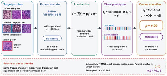
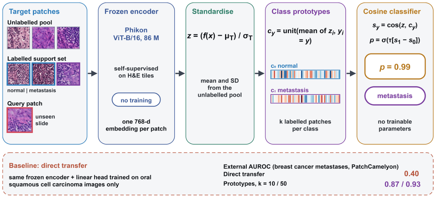
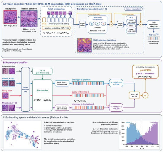
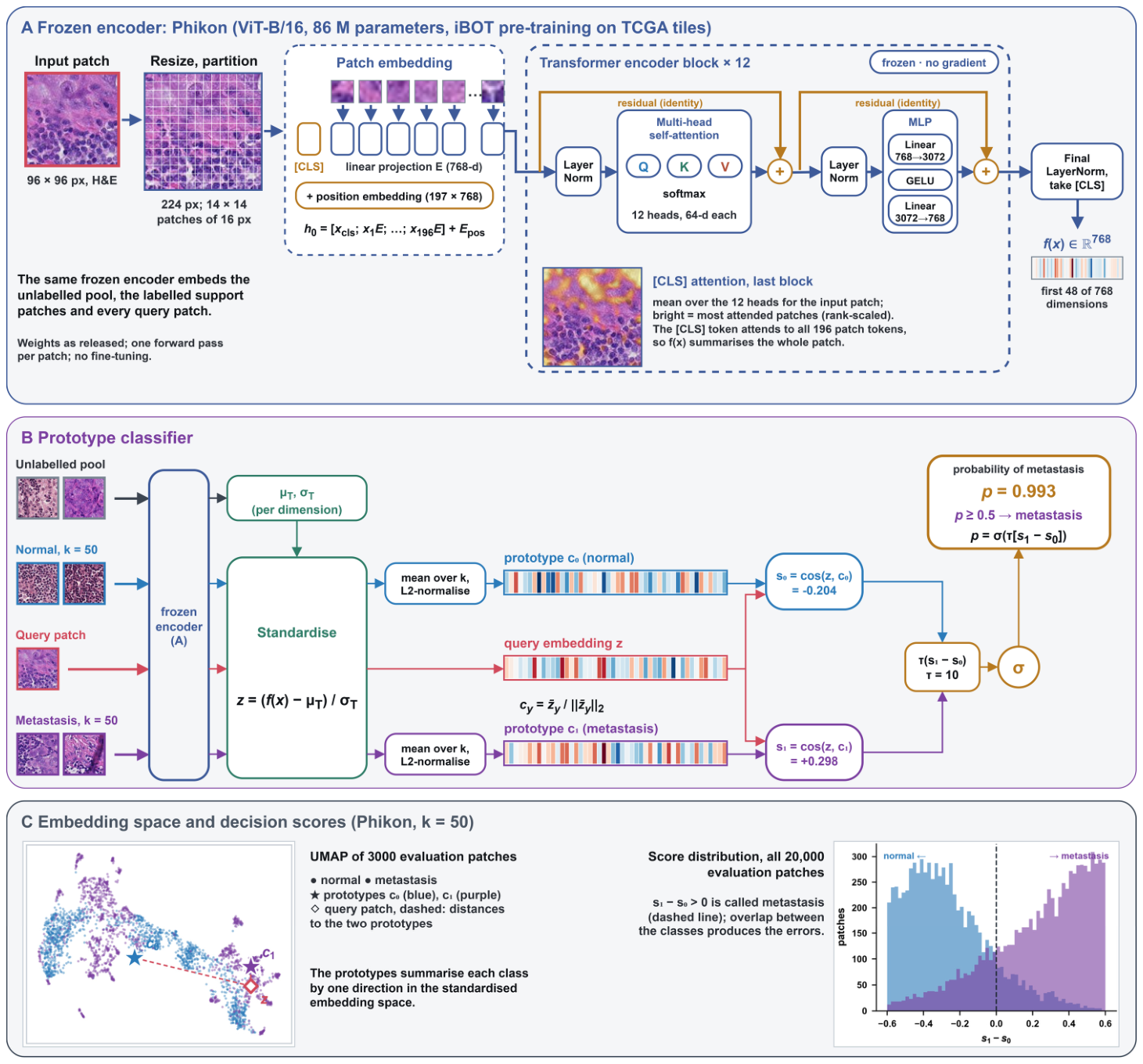
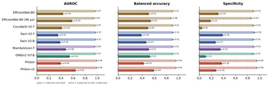
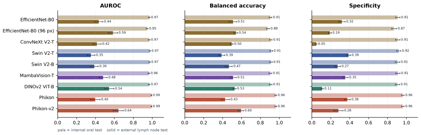
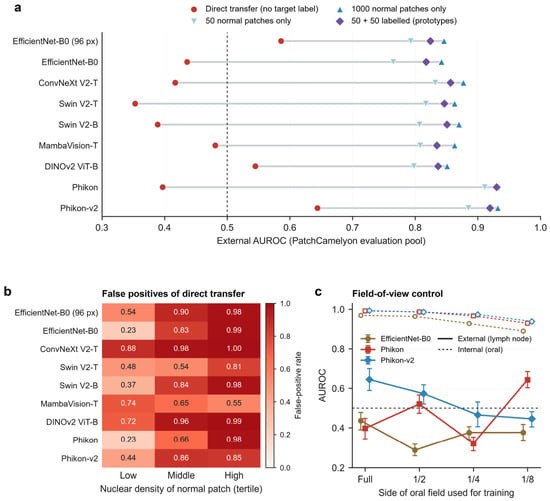
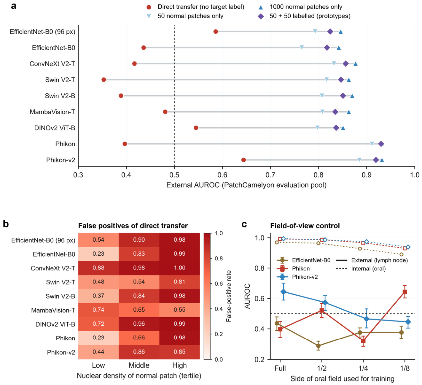
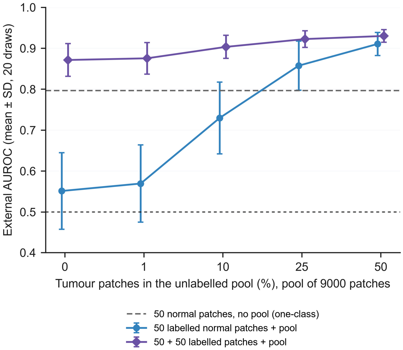
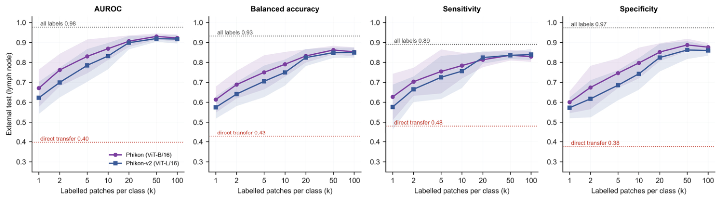
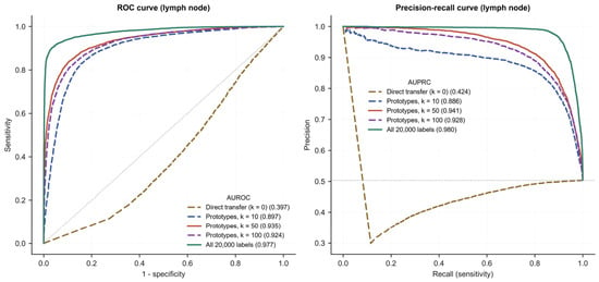
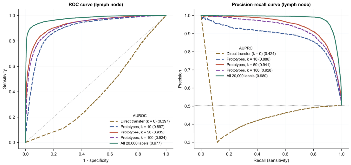
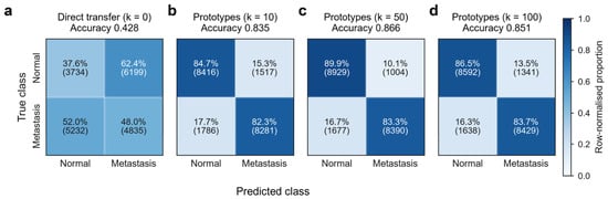
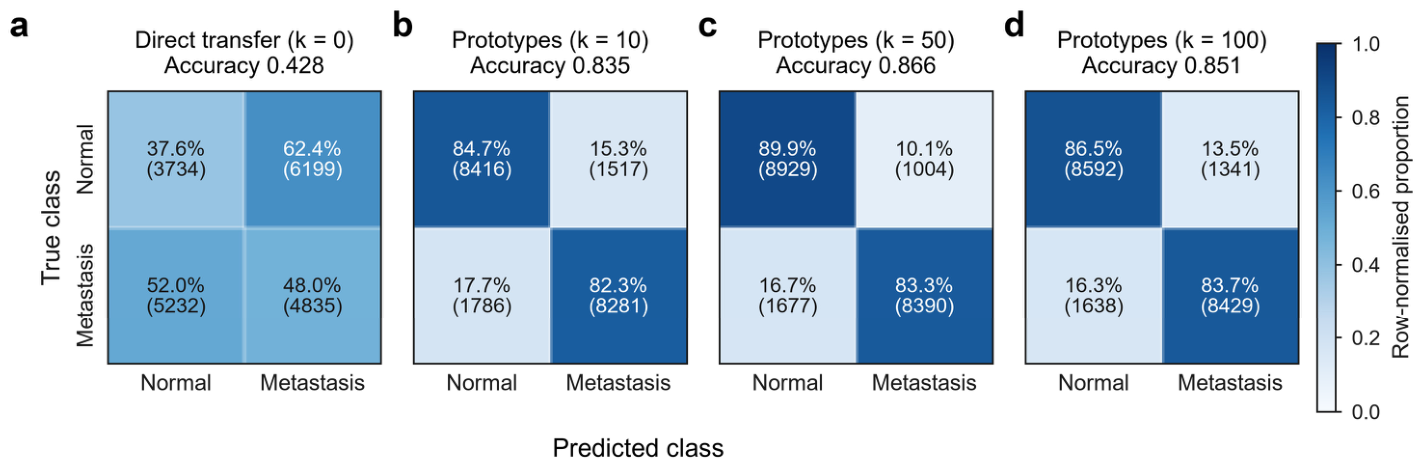
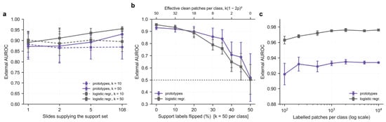
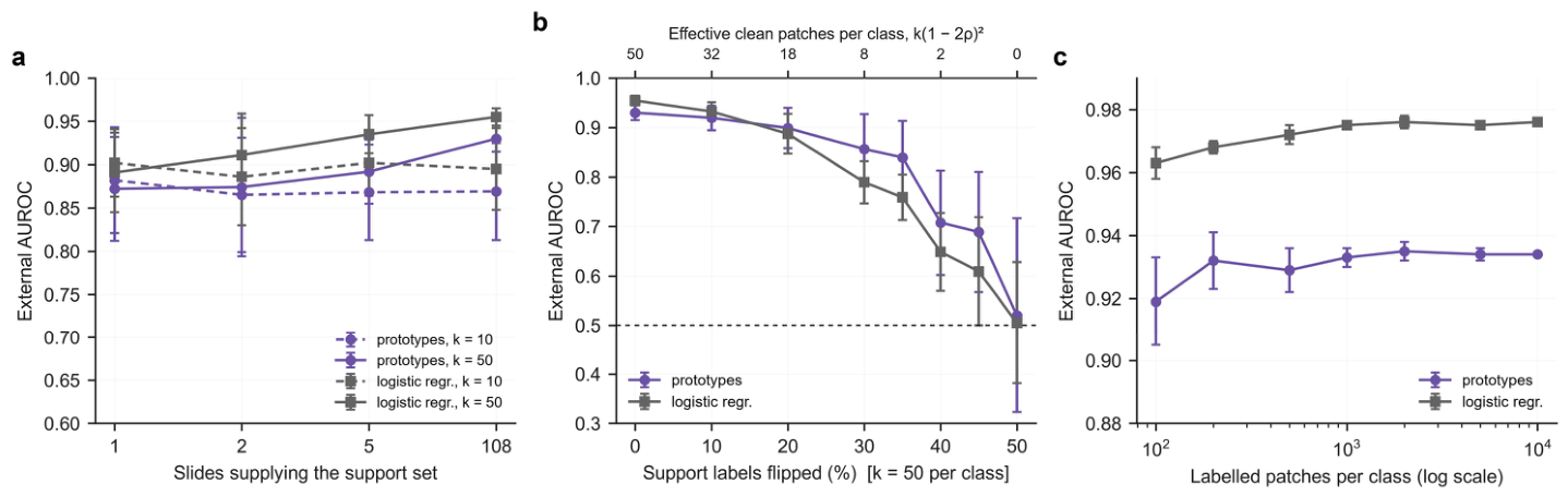
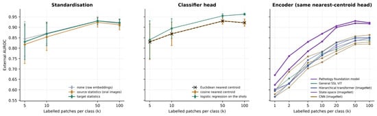
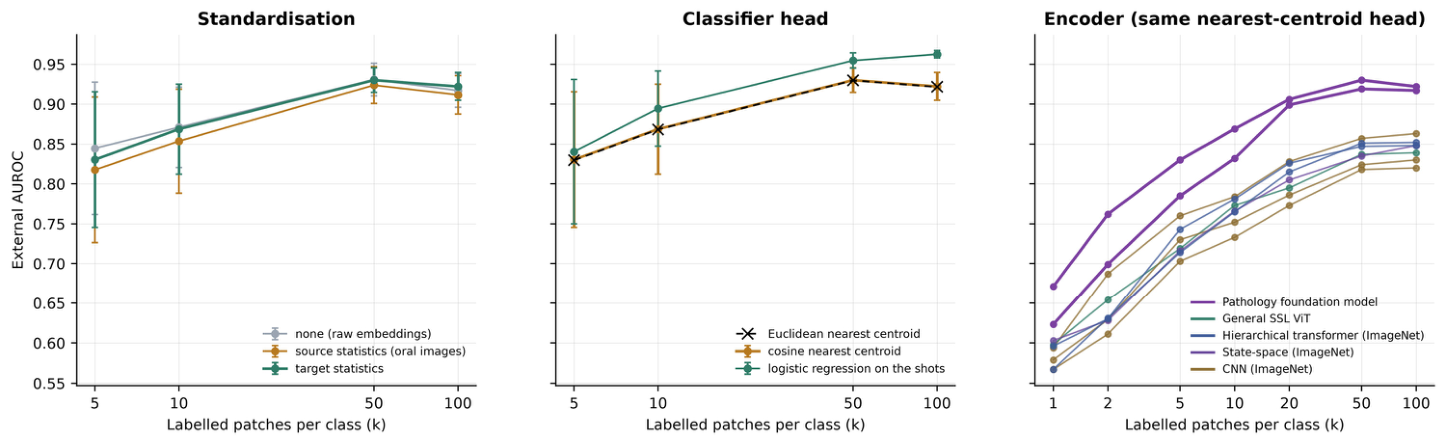
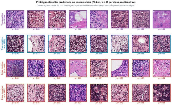
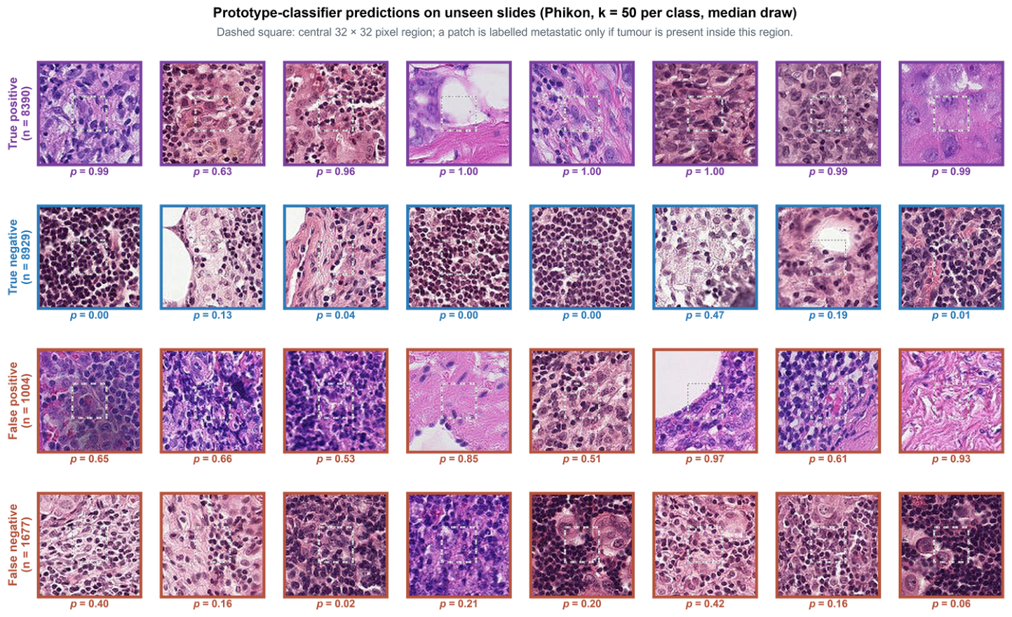
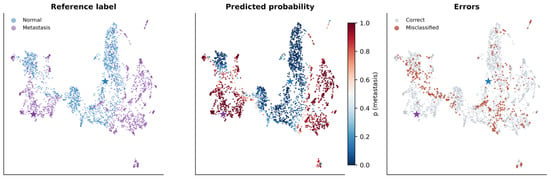
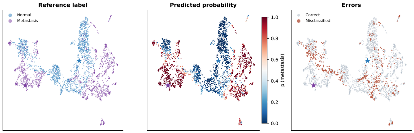
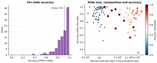
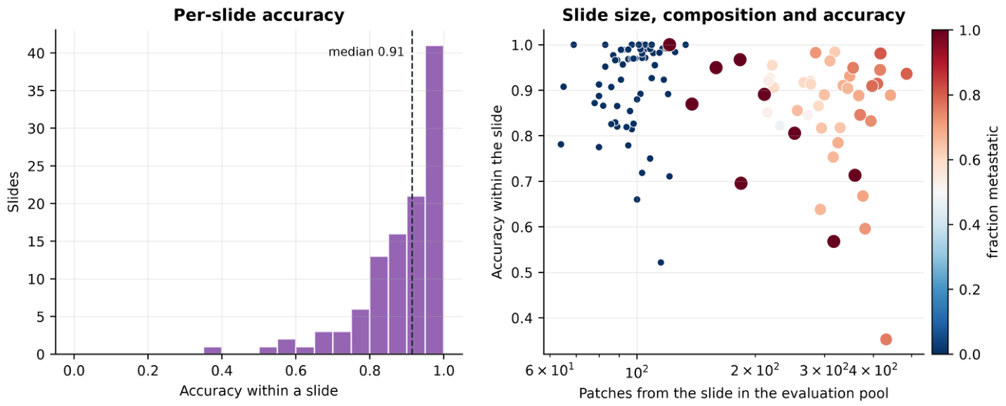

Disclaimer/Publisher’s Note: The statements, opinions and data contained in all publications are solely those of the individual author(s) and contributor(s) and not of MDPI and/or the editor(s). MDPI and/or the editor(s) disclaim responsibility for any injury to people or property resulting from any ideas, methods, instructions or products referred to in the content. |
© 2026 by the authors. Licensee MDPI, Basel, Switzerland. This article is an open access article distributed under the terms and conditions of the Creative Commons Attribution (CC BY) license.