


Abstract
Machine learning can predict microfluidic droplet size, but the best-performing model for familiar channel geometries may not suit new geometries. Using published flow-focusing droplet data, we compared model recommendations from different evaluation schemes and their predictive outcomes on unseen geometries. With matched training and test record counts in the main dataset, holding out all records of selected geometries increased the gradient-boosted tree model’s mean absolute diameter error from 8.29 to 12.22 µm, a 47.4% increase over random splitting, and reversed its ranking relative to the random forest. We then tested models recommended by the two validation schemes on the same geometries unseen during training. Those selected by geometry-grouped validation had an 8.2% lower mean absolute diameter error, averaged with equal weight per geometry, than those selected by random validation. Fixed random forest had the lowest error. In both candidate sets, operating conditions recommended by models selected through grouped validation had a smaller mean absolute deviation of measured diameter from the target than those recommended using random validation. At ±10% tolerance, the attainment ranking of the two rules depended on the candidate set. Model recommendations for new geometries should therefore be assessed on the same unseen geometries, while target-size recommendations require direct evaluation of the proportion meeting the specified tolerance.
1. Introduction
Predictable droplet size is important for applications such as single-cell analysis and materials synthesis [1]. In a flow-focusing device, the dispersed liquid enters the surrounding continuous phase and breaks into droplets at the junction [2]. Channel geometry, fluid properties, and the flow rates of both phases jointly influence the final diameter [3,4,5]. Machine learning can predict droplet size from these inputs to assist in selecting operating conditions [6]. A key practical question is whether the model that performs best on other operating conditions in familiar geometries is also suitable for geometries absent from training.
Design Automation of Fluid Dynamics (DAFD) is an established prediction and design platform [7], with subsequent work addressing operating range and stability optimization [8]. DAFD 3.0 also conducted blind predictions and experimental tests on geometries, fluids, and materials unseen during training [9]; earlier work demonstrated transfer to new fluid combinations using limited data [7]. Our main analysis uses its publicly available single-emulsion experimental records. Other studies have addressed surfactants, non-Newtonian fluids, heterogeneous microchannels, and prediction-assisted design [10,11,12,13,14,15,16]. Hormozinezhad et al. [11] used the target droplet size and fluid properties, among other inputs, to predict the required flow rates of both phases. They tested their model on conventional holdout data and on non-Newtonian fluids unseen during training.
Grouped validation is an established approach for handling dependence among observations [17,18,19,20,21]. Random splitting and complete geometry holdout address different tasks: the former allows existing data from a geometry to support prediction at other operating conditions in that geometry, whereas the latter requires prediction for geometries entirely absent from training.
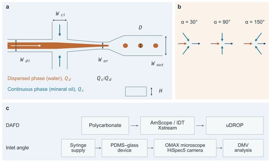
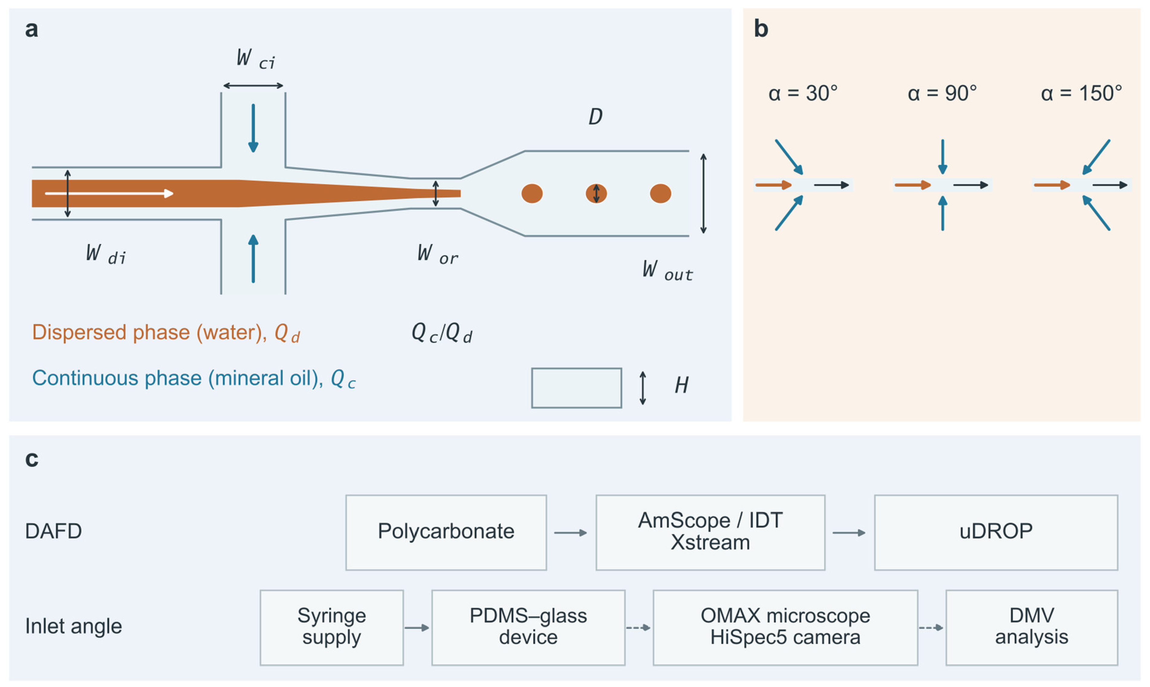
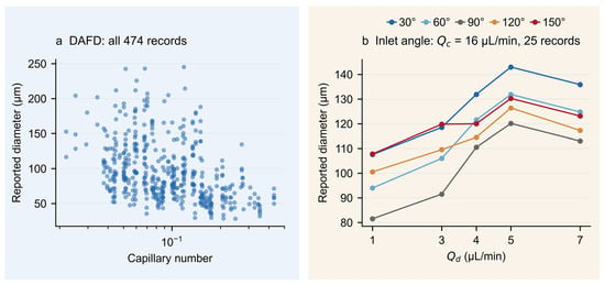
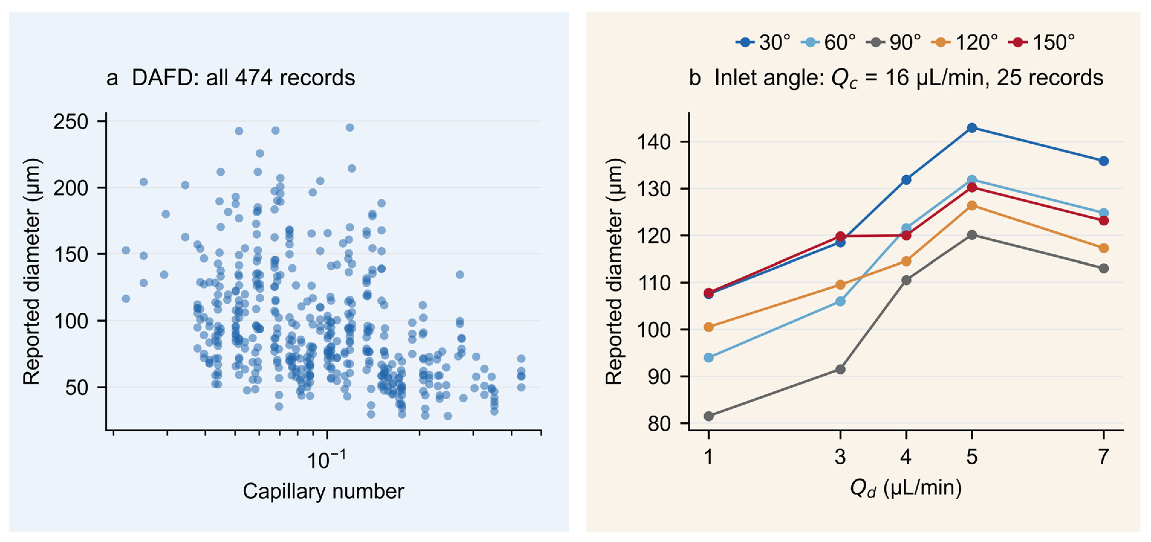
Inlet tilt angle provides another observable change in geometry. Talebjedi et al. [22] investigated how continuous-phase inlet direction affects droplet formation in a water–mineral oil system. They developed predictive models for size, generation frequency, and quality metrics, and performed operating-condition optimization and flow-regime classification. Their published records cover five angles and 25 combinations of operating conditions. The inlet configurations and data-acquisition context are shown in Figure 1, and representative source diameter records are shown in Figure 2b.
Figure 1.
Physical variables in flow-focusing droplet formation and acquisition workflows in the source studies. (a) Generic flow-focusing schematic: Wdi, Wci, Wor, Wout, and H denote the dispersed-phase inlet width, continuous-phase inlet width, orifice width, outlet width, and channel depth, respectively; D denotes droplet diameter, and Qc/Qd is the continuous-to-dispersed-phase flow-rate ratio. (b) Inlet-angle configurations of 30°, 90°, and 150°, with α retaining the source notation. (c) Device materials, microscopy, and diameter-extraction workflows for the two sources. The inlet-angle row also shows the connection between syringe-based fluid delivery and the device. The main-data row shows the device material reported for DAFD 3.0 [9] and follows the earlier acquisition workflow [7]; the inlet-angle row corresponds to the 30°, 90°, and 150° experiments described in [22]. Solid arrows in the inlet-angle row indicate fluid delivery, while dashed arrows indicate imaging and image-processing relationships. uDROP and DMV are the image-processing tools used by the sources. The schematics were independently drawn from the source descriptions, are not to scale, and do not specify how Qc is allocated among branches.
Figure 2.
Published diameter records in the main and supporting datasets. (a) Diameter versus capillary number for all 474 DAFD records, with geometry and flow-rate ratio varying simultaneously. Redrawn from the SE-diameter records in the “Figure 1 and Figure 2” worksheet of the official Source Data of [9], under CC BY 4.0 (https://creativecommons.org/licenses/by/4.0/, accessed on 16 November 2026), with a changed layout and unchanged numerical values. (b) All 25 records spanning the five angles at 16 µL/min, the middle of the five Qc levels, from Supplementary Tables S1–S3 of [22]. Each point represents one published operating-condition record; lines are visual guides only. All 125 records are shown in Figure S7.
Prior studies have evaluated the predictive performance of microfluidic models on unseen geometries or fluids [9,11]. Selecting a model for a new channel requires understanding how the data split changes candidate rankings and how the resulting recommendations perform on the same new channel.
Using matched training and test record counts in the main DAFD dataset, we first compared diameter prediction errors and model rankings under random splitting and complete geometry holdout. We used the inlet-angle data to assess whether the ranking change also occurred under another definition of configuration groups, holding out all records for one angle at a time. We then compared the models selected by the two validation rules on the same held-out geometries, including fixed models as controls.
In the DAFD dataset, we also explore the target-size recommendation performance of the selected models and the effects of five-point calibration per geometry on prediction error and size attainment.
2. Materials and Methods
2.1. Experimental Sources and Measurement Data
The main dataset contains 474 publicly available single-emulsion operating-condition records from DAFD [9]. The source experiments used 43 polycarbonate flow-focusing designs, deionized water, and NF 350 mineral oil, with reported diameters of approximately 25–250 µm. The earlier acquisition workflow [7] used an AmScope stereomicroscope, an IDT Xstream high-speed camera, and uDROP image processing. We use the diameters reported by the source. The inputs and diameters of all 474 records were matched individually to the official Source Data of [9], as detailed in Section S1.
The inlet-angle source study [22] used water as the dispersed phase and mineral oil as the continuous phase, and reported a channel width of 150 µm and depth of 60 µm. Its 30°, 90°, and 150° devices were fabricated from polydimethylsiloxane (PDMS) and bonded to glass. A KD-scientific syringe pump and Hamilton 1 mL gastight syringes supplied the fluids. A HiSpec5 4G Mono camera and an OMAX inverted microscope were used for imaging, followed by frame-by-frame analysis with Droplet Morphometry and Velocimetry (DMV). Figure 1 shows the physical variables and acquisition context for the two sources.
The supporting comparison uses 125 full-factorial design records in Supplementary Tables S1–S3 of [22]. The original authors reported them as experimental points but did not separately describe how the 60° and 120° records were obtained. We retain the source attribution and use these records for a supporting comparison of published data. The five angles are 30°, 60°, 90°, 120°, and 150°, each sharing the same 25 operating conditions. The dispersed-phase flow rate Qd takes values of 1, 3, 4, 5, and 7 µL/min; the source-reported continuous-phase flow rate Qc takes values of 10, 13, 16, 18, and 20 µL/min.
We joined Supplementary Tables S2 and S3 of [22] one-to-one by experiment number, with flow-rate levels taken from Supplementary Table S1 of that study. Reconstruction and precision checks are detailed in Section S5.1. The source variables α and Qc were retained, and the flow-rate ratio was Qc/Qd. Figure 2 shows all 25 corresponding records at 16 µL/min, the middle of the five Qc levels; Figure S7 shows all 125 records.
2.2. Variables, Geometry Groups, and Prediction Models
DAFD geometries are defined by the orifice width Wor and four ratios: channel depth H/Wor, continuous-phase inlet width Wci/Wor, dispersed-phase inlet width Wdi/Wor, and outlet width Wout/Wor. Widths and depth are in µm, and the ratios are dimensionless. Varying flow rates while keeping the geometric parameters unchanged produces different operating-condition records within the same geometry group. These five parameters assign the 474 records to 35 geometry groups, matching the grouping obtained from the original physical dimensions. Complete geometry holdout uses these groups as its units. The flow-rate ratio Qc/Qd, capillary number, and viscosity ratio of the two phases complete the eight prediction inputs; these three inputs are not used to define geometry groups. The capillary number describes the relative magnitudes of viscous and interfacial-tension effects. Source fields and reconstruction are detailed in Section S1.
For the main dataset, the prediction target was droplet diameter normalized by the orifice hydraulic diameter Dh. Predictions were converted back to µm using Equation (1).
In Equation (1), Wor is the orifice width, H is the channel depth, and D is the droplet diameter reported in the source. Dnorm is the normalized diameter, Dnorm,pred is its model prediction, and Dpred is the predicted diameter restored to physical units.
Gradient-boosted trees (XGBoost [23]), random forests (RF [24]), and multilayer perceptrons (MLP), all with fixed configurations, used the same DAFD inputs and prediction target. For the angle dataset, the angle, Qc/Qd, and Qc were used to predict unnormalized diameter; the RF analysis was a targeted post hoc extension. Standardization parameters for each fit were estimated from the training data only. Each model used the same fixed configuration under R and G. XGBoost followed the core settings of DAFD 3.0 [9]. The basis for each configuration and its parameters are given in Supplementary Section S2.3 and Table S3A,B.
2.3. Evaluation Protocols for Seen and Unseen Geometries
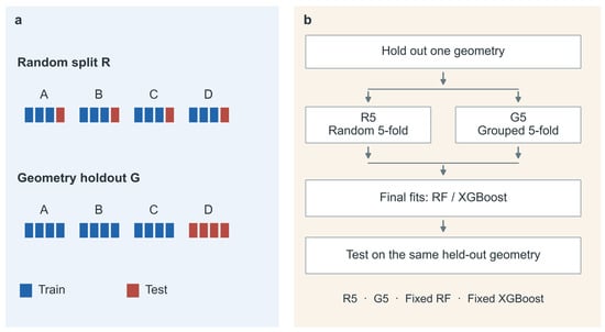
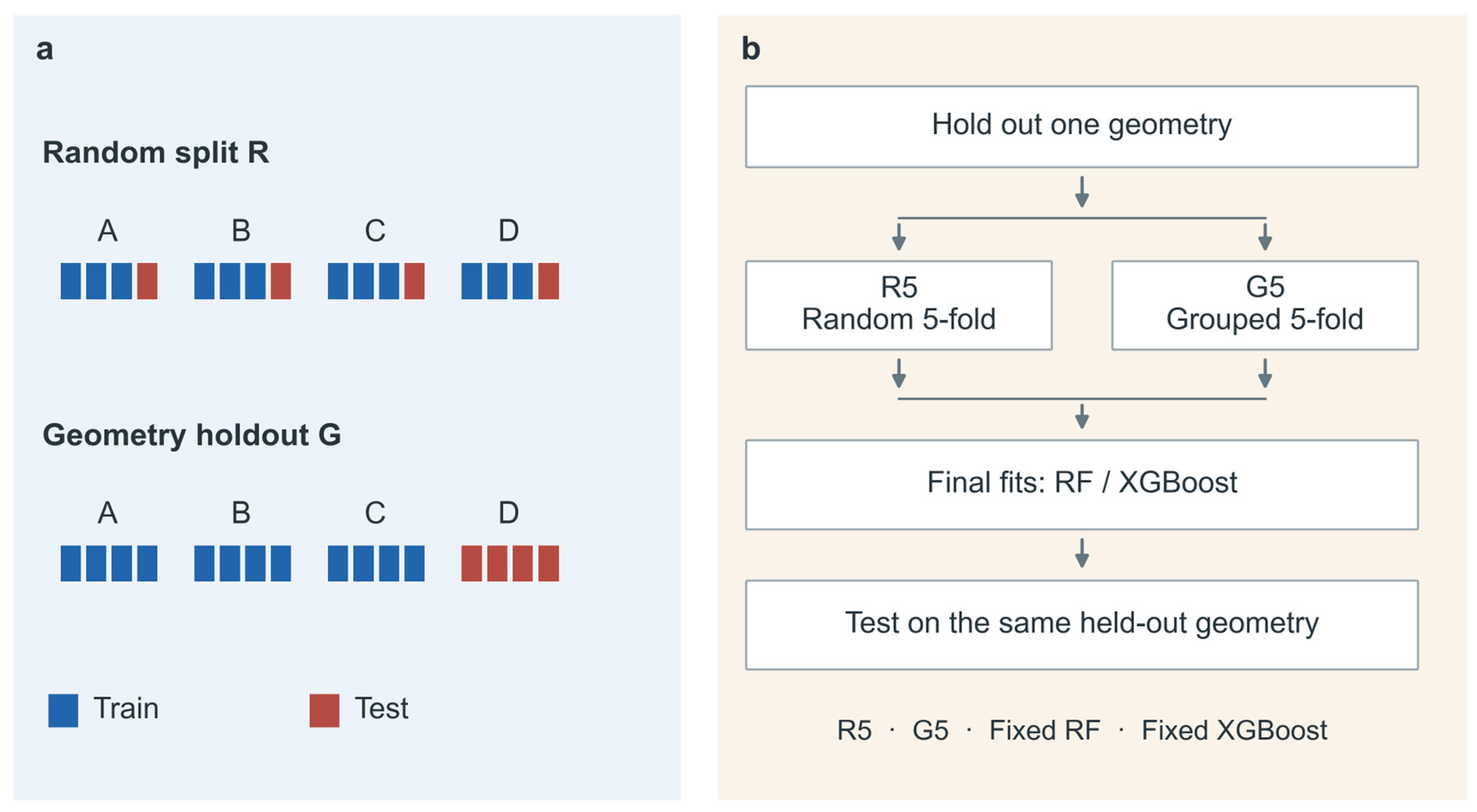
Random evaluation R split individual records 80/20 and primarily assessed prediction at other operating conditions of familiar structures. Complete geometry evaluation G held out all records of each test geometry, assessing structures absent from training. To control sample size, both protocols used 379 training and 95 test records, with 100 splits each. The sampling rules and seeds are given in Section S2 and Table S3B.
To compare how close the test conditions were to the training data under the two protocols, we standardized the inputs using the statistics of the corresponding training set and calculated the Euclidean distance from each test record to its nearest training record. We also computed distances separately for geometry and operating inputs to determine which input category showed the larger difference in coverage (Table S8D).
Grouped five-fold evaluation and leave-one-geometry-out evaluation (LOGO) were also used to examine errors under alternative complete geometry partitions, as detailed in Section S4.3.
To examine whether model rankings changed when prediction shifted from seen to unseen angles, we compared 100 random 80/20 splits with leave-one-angle-out evaluation (LOAO) on the inlet-angle dataset. In each LOAO round, all 25 records at one angle formed the test set, and the 100 records at the other four angles were used for training. All angles shared the same 25 flow-rate combinations, so this comparison assessed prediction for an unseen inlet direction at flow-rate combinations already represented in training. Within each split, the candidate models used identical training and test records. Full rules are provided in Section S5. Table 1 and Figure 3 distinguish final evaluation from internal selection.
Table 1.
Record counts, geometry groups, and evaluation tasks for the two datasets.
Figure 3.
Relationship between test-set partitioning and model selection. (a) Random splitting R assigns records to training and test sets, allowing the same geometry in both; complete geometry holdout G withholds all records of each test geometry. Letters denote geometries, and blue and red denote training and test records, respectively. Record counts are schematic. (b) Each round first holds out one geometry. Within the remaining geometries, random five-fold validation R5 and geometry-grouped five-fold validation G5 each select between RF and XGBoost. Both candidates are then refitted on the same outer training records. R5, G5, fixed RF, and fixed XGBoost use predictions from these two final fits for comparison on the same held-out geometry.
2.4. Testing Two Model-Selection Rules on the Same Unseen Geometries
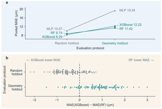
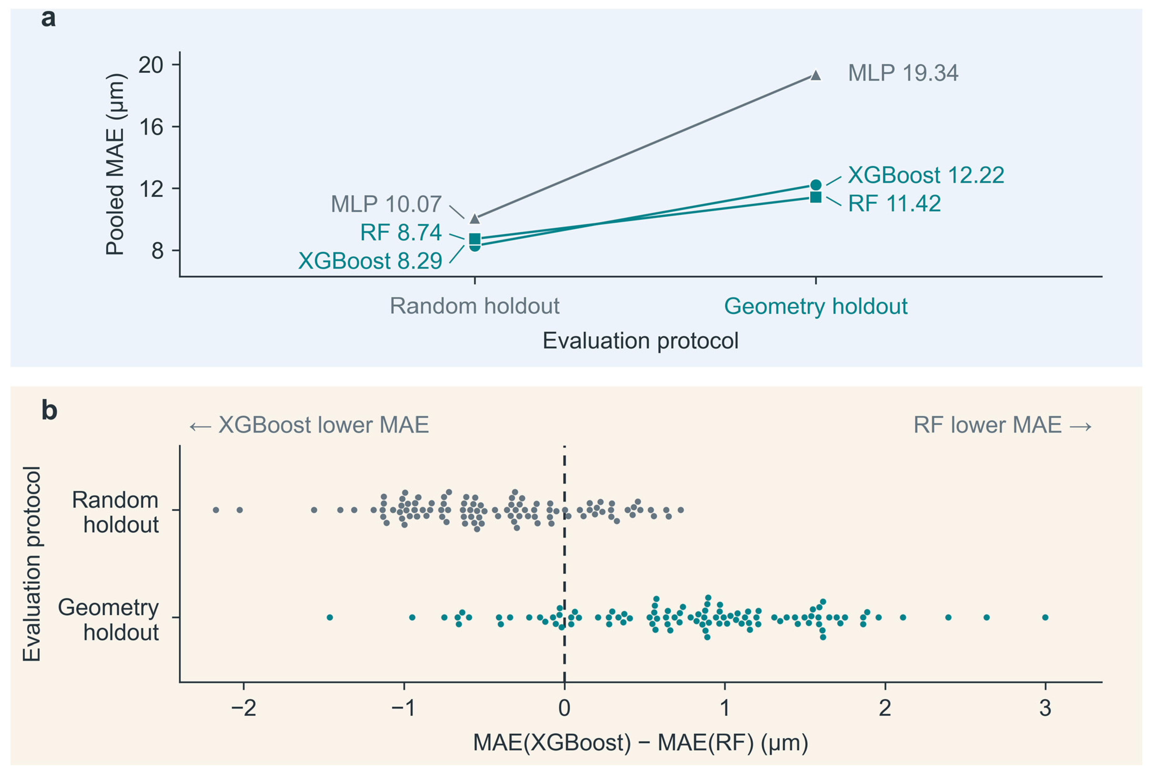
R and G used different test records and revealed differences in error and ranking between the two evaluation settings. To directly compare the models recommended by the two validation rules, we used nested evaluation to separate internal model selection from final testing [25,26]. This nested comparison was a retrospective extension conducted after inspection of the early DAFD results. In the early comparison, the MLP had pooled MAEs of 10.07 µm under R and 19.34 µm under G, ranking third in both schemes. The nested comparison focused on RF and XGBoost, whose rankings reversed. Their configurations, scoring rule, and partition rules were fixed before fitting models for the extension. Each round held out one entire geometry. Within the remaining 34 geometries, random five-fold validation R5 and geometry-grouped five-fold validation G5 each selected between RF and XGBoost.
The record count in each R5 fold matched that of the corresponding G5 fold. Each candidate predicted every internal validation record once. Mean absolute error was first calculated within each validation geometry and then averaged with equal weight across the 34 geometries; both rules selected the candidate with the lower score. Diameter labels from the held-out geometry were not used for selection.
After internal selection, RF and XGBoost were each fitted on all records from the remaining 34 geometries and used to predict the held-out geometry. R5 and G5 determined only which set of predictions to use, sharing the same final RF and XGBoost predictions in each round. This common test therefore measured the prediction differences resulting from the two model-selection recommendations.
Always using RF and always using XGBoost served as two controls to test whether selecting a model for each geometry outperformed using one fixed model. All 35 geometries were used in turn for final testing, including geometries represented by a single record. Ten additional internal partition arrangements were specified in advance to examine whether the direction of the comparison depended on a particular fold assignment; final tests and candidate predictions remained unchanged, as detailed in Section S3. Preprocessing, RF, and MLP were implemented using scikit-learn 1.6.1 [27]. XGBoost was implemented using the XGBRegressor interface provided by xgboost 3.4.1. Model hyperparameters and random seeds are listed in Table S3A,B, and Section S12 describes the computational implementation and reproducibility checks.
2.5. Error Metrics, Units, and Aggregation Weights
Mean absolute error (MAE) measures the average absolute difference between the predicted diameter and the diameter reported in the source, in µm, as defined in Equation (2).
In Equation (2), n is the number of test predictions included in the calculation, Di is the diameter of record i, and Dpred,i is the corresponding predicted diameter.
R and G each used 100 repeated splits with 95 test records per split; the main results pooled the errors from these 9500 predictions. Because the same record could be tested repeatedly, we also first averaged repeated errors for each original record and then averaged equally across records to check whether repeated inclusion affected the conclusions. Each record was tested once in grouped five-fold evaluation and LOGO.
To assess whether the ranking depended on individual splits, we compared RF and XGBoost on the same test set within each split and summarized the paired differences separately for random splitting and complete geometry holdout. Table S8C reports variation across splits and approximate 95% intervals for the means conditional on the fixed dataset.
For the common model-selection comparison, errors were first averaged within each geometry and then averaged with equal weight across the 35 geometries, preventing geometries with more records from dominating the conclusions. Root mean square error (RMSE), the coefficient of determination (R2), and mean absolute percentage error (MAPE) were secondary metrics. RMSE and R2 were calculated directly from the corresponding predictions, and relative changes were calculated using unrounded values.
2.6. Operating Condition Selection for Target Sizes and Five-Point Calibration
To assess whether models could select operating conditions that met target-size requirements, we performed an exploratory analysis using existing experimental data. We retained 29 geometries with at least ten records each and compared strategies using four equally spaced illustrative targets of 75, 100, 125, and 150 µm for each geometry, yielding 116 tasks. The outer model selections and predictions were reused without refitting. Each rule selected the candidate operating condition whose predicted diameter was closest to the target. Its archived measured diameter was then used to assess the deviation from the target and whether the tolerance was met. For example, the acceptable range for a 100 µm target at ±10% was 90–110 µm.
The primary attainment criterion was |Dchosen − Dtarget|/Dtarget ≤ 0.10; a tolerance of 0.20 was also reported. Here, Dchosen is the source-reported measured diameter under the selected operating condition, and Dtarget is the specified target diameter.
To define a common candidate pool for subsequent operating condition selection, we used the record partition described in Section S8: five calibration records were reserved for each of the 29 geometries, leaving 310 records as the common candidate set C. This let us assess, on the same candidate conditions, recommendations made without diameter labels from the new geometry and the effect of calibration after five labels became available. All 455 records from these 29 geometries were also used. To examine the effect of candidate composition at a fixed candidate count, we reserved five records uniformly at random within each geometry to construct 1000 sets of 310 candidate records each. All strategies shared the same candidate records within each draw and reused the original model selections and predictions.
All selection rules and fixed-model controls used the same candidates, targets, and tolerances. Ties were resolved successively by operating inputs, remaining inputs, and record identifier. Target deviation compared the measured diameter of the selected condition with the target, whereas prediction error compared predicted and measured diameters. We classified each target as within or outside the measured diameter range for its geometry in the corresponding candidate set, reported attainment separately for the two groups, and checked whether each task had a candidate operating condition within tolerance. Operating condition selection was restricted to candidates with existing measurements, and the 116 target tasks were compared descriptively. Full rules are provided in Section S7.
Five-point calibration used fixed RF and the same 29 geometries without retraining the base model. The five points for each geometry were selected using operating inputs only: a point near the input-space center was chosen first. At each subsequent step, we calculated the Euclidean distance from each candidate point to its nearest selected point and chose the candidate with the largest such distance. The logarithmic inputs, standardization, and tie-breaking rules are detailed in Section S8.
After accessing the five diameters, the median residual, measured minus predicted diameter, was added to all candidate predictions for that geometry to correct the overall offset. A target operating condition was then selected from C. The five labels were available for calibration, while measured labels in C were used only for final evaluation. The same five points were shared by the four targets for each geometry, totaling 145 labels. This comparison tested whether a small number of measurements from a target geometry could improve diameter predictions at its remaining operating conditions and the proportion of recommendations meeting the target-size tolerance.
3. Results
3.1. Diameter Prediction Errors and Model Rankings in the DAFD Dataset
Random evaluation mainly tested other operating conditions in familiar geometries. Across the 100 random splits, 9434 of the 9500 test predictions (99.31%) were for geometries represented in the corresponding training set. Under complete geometry holdout, the median distance in the joint input space from a test record to its nearest training record increased from 0.512 to 1.416. The difference was most apparent in the geometry inputs. The median nearest-neighbor distance for the operating inputs alone did not increase (Table S8D). The mean absolute diameter error of XGBoost was 8.29 µm under random splitting and 12.22 µm under complete geometry holdout, a 47.4% increase (Table 2). Giving each original record equal weight, MAE remained higher under complete geometry holdout than under random splitting (Table S9). The other geometry holdout schemes also yielded higher MAEs than random splitting (Table 2 and Figure S8).
Table 2.
Diameter prediction errors of XGBoost under four evaluation schemes for the DAFD dataset.
The model ranking also reversed with the evaluation task (Figure 4). When the models were compared on the same test set within each split, the MAE of XGBoost was on average 0.449 µm lower than that of RF under random splitting and 0.795 µm higher under complete geometry holdout. Most splits supported the overall ranking for their protocol, with the opposite order in some splits (Table S8C). Aggregation with equal weight per original record retained the ranking reversal, and MLP ranked third under both schemes (Table S9).
Figure 4.
Comparison of fixed prediction pipelines on the DAFD dataset. (a) Pooled MAE for XGBoost, RF, and MLP, based on 9500 test predictions per scheme. (b) The difference in error between XGBoost and RF within each of the 100 splits per scheme; positive values favor RF. Candidates share test records within a split, but split indices do not define paired comparisons between R and G.
The two evaluations would recommend different models. The next section compares the prediction errors resulting from the two recommendations on the same held-out geometries.
3.2. Model Selection on Common Unseen Geometries
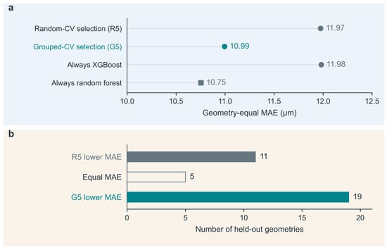
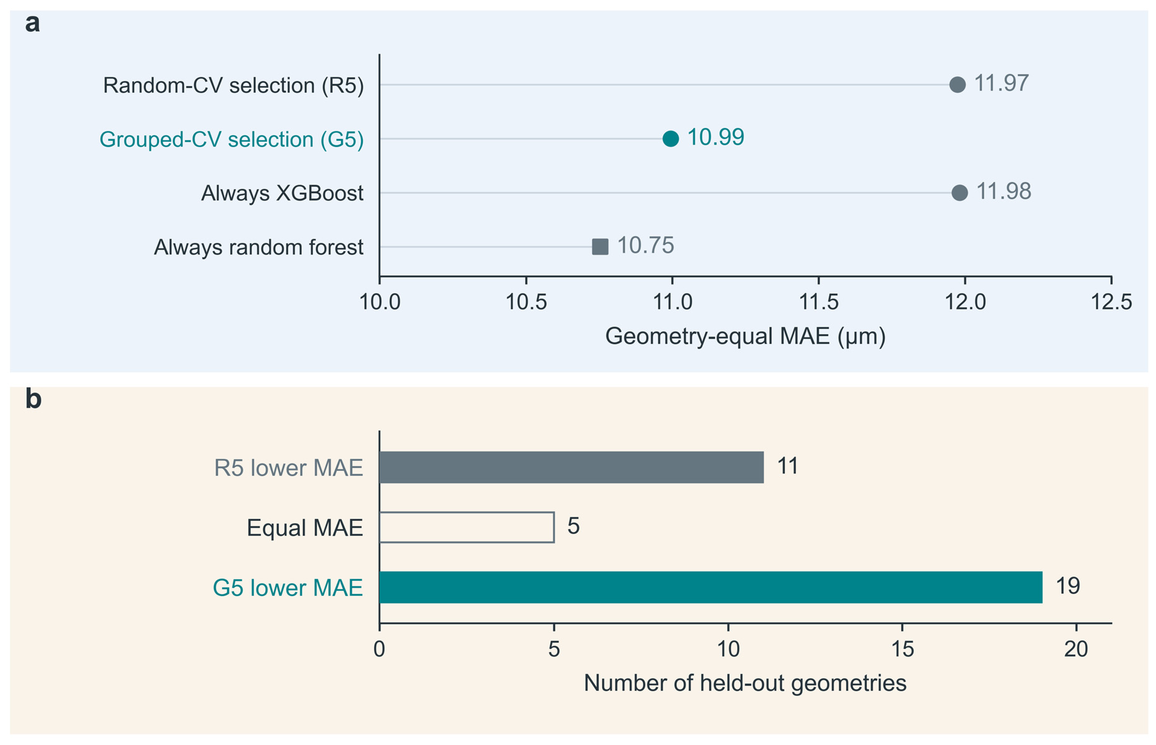
Across the 35 common held-out geometries, the geometry-equal MAE was 10.99 µm for G5-selected models, 8.2% lower than the 11.97 µm for R5 (Table 3). The two rules recommended different models for 30 geometries. In each case, R5 selected XGBoost and G5 selected RF.
Table 3.
Prediction errors of the models selected by the two validation rules and of fixed models on common unseen geometries.
Compared with R5, G5 had a lower error for 19 geometries, a higher error for 11, and the same error for 5 (Figure 5 and Table S5). Aggregation with equal weight per record also retained the reduction in mean error.
Figure 5.
Model selection on common unseen DAFD geometries. (a) Outer MAE averaged with equal weight per geometry for R5, G5, and the fixed-model controls; all strategies share the final candidate predictions. (b) R5 had the lower error for 11 geometries, the errors were equal for 5, and G5 had the lower error for 19. All 35 geometries were retained, including three with a single record. Results for individual groups are provided in Figure S1 and Tables S4 and S5.
The lower mean error of G5 relative to R5 arose from selecting RF more often. Compared with fixed RF, G5 switched to XGBoost for only two geometries, and both switches increased the error. Fixed RF therefore had the lowest mean error on these held-out geometries (Table 3 and Table S5).
Across ten additional internal partition arrangements, the mean error of G5 remained 0.53–1.11 µm lower than that of R5, while fixed RF achieved the same or a lower error (Table S7A).
3.3. Supporting Comparison Using the Angle Dataset
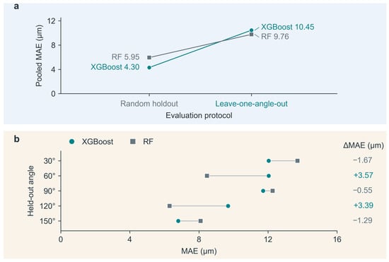
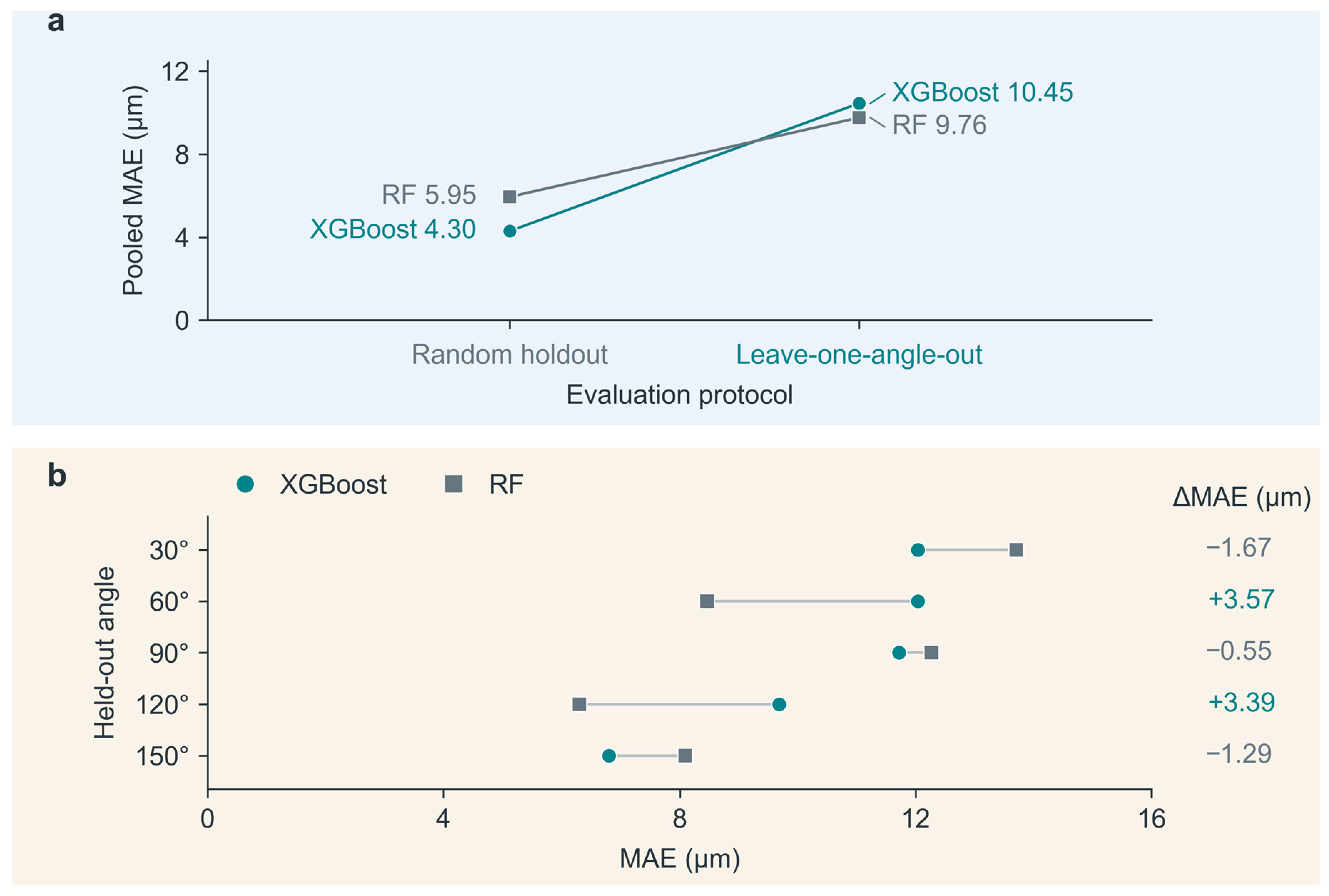
The inlet-angle data also showed the same overall ranking reversal. Under random evaluation, the MAE of XGBoost was 4.30 µm, lower than the 5.95 µm of RF. Under complete angle holdout, RF yielded 9.76 µm, lower than the 10.45 µm of XGBoost (Figure 6). This result supports the evaluation-dependent ranking change observed in the DAFD dataset under another configuration grouping. At individual angles, RF led at 60° and 120°, whereas XGBoost led at the other three angles, showing that the overall ranking did not imply the same advantage at every angle. Summary and angle-specific results are provided in Tables S12A,B and S13A,B.
Figure 6.
Supporting model comparison across inlet angles. (a) Pooled MAE under random holdout (2500 test predictions) and LOAO (125 predictions). (b) Candidate MAE at each held-out angle, with 25 records per angle; positive differences between XGBoost and RF favor RF. The RF analysis was a targeted post hoc extension. Complete results are provided in Table S13A,B.
3.4. Target-Size Attainment and Five-Point Calibration
For model-based recommendations of operating conditions, mean absolute deviation measures how close the measured diameters of the selected conditions are to the targets. In the common candidate set C, the mean absolute deviation decreased from 23.29 µm for R5 to 20.97 µm for G5. Attainment within ±10% was also slightly higher for G5 than for R5, by 1.7 percentage points (Table 4).
Table 4.
Numbers of target-size tasks meeting the tolerance under two candidate ranges. Each strategy was evaluated on 116 tasks.
When all measured operating conditions were available, the measured diameters of conditions selected by G5 were still closer to the target on average, with a slightly lower attainment rate than R5 at ±10% tolerance (Table 4 and Table S16). Thus, the attainment ranking was reversed between the two candidate sets. In C, the two rules met the tolerance for the same number of targets within the measured range. The small overall difference arose from targets outside this range. Table S16D gives the full results by stratum.
With the number of candidate conditions per geometry fixed, changing which conditions were retained could still change the attainment ranking of the two model-selection rules at ±10% tolerance. At ±20% tolerance, G5 attained more targets than R5 in most candidate sets, with a median difference of four tasks. Compared with fixed RF, the median difference in the number of targets attained by G5 was zero at both tolerances (Table S16C).
If a few measured diameters are available for each new geometry, they can be used to correct the model’s prediction offset. After calibrating fixed RF with the five measured diameters reserved for each geometry, the geometry-equal MAE in candidate set C decreased from 10.77 to 8.95 µm, a reduction of 16.9%, without retraining the base model.
In the same candidate set, the attainment rate within ±10% increased from 37.1% to 40.5% (Table S17). This comparison describes how calibration with five measurements from the target geometry affects prediction and recommendation for the remaining measured candidate conditions.
4. Discussion
DAFD 3.0 used blind predictions and experiments to evaluate performance on unseen geometries, fluids, and materials [9]. Hormozinezhad et al. tested flow-rate predictions for the two phases on conventional holdout data and on unseen non-Newtonian fluids [11]. We extended these assessments by comparing how two evaluation designs affect model rankings and by measuring the errors resulting from their recommendations on the same unseen geometries. The design follows the principle of partitioning data according to the structure of the observations [18,21] and evaluates each selection rule alongside fixed models.
To predict a new flow-rate combination in an existing channel, the training set can retain other measured conditions for that geometry, with the test conditions held out by record. To predict channel structures unseen in training, entire test geometries should be held out, with models recommended by the selection rules and fixed models compared on the same held-out geometries. When interpreting performance under new conditions, it is important to assess how well the training data cover the test conditions [28]. We measured this coverage using nearest-neighbor distances for the geometry and operating inputs separately.
Of the two model-selection rules, G5 more often recommended RF, which had lower average error on these unseen geometries. Fixed RF had the lowest error among the controls in this dataset. For new designs, grouped evaluation helps select models for the intended prediction task and uses fixed models as benchmarks for assessing the value of geometry-specific selection.
Prediction error and the operating-condition decisions it supports need to be evaluated separately [29,30]. In this study, attainment depended on the specified tolerance, the availability of an acceptable operating condition in the candidate set, and whether the model selected it. The effectiveness of operating-condition recommendations should therefore be assessed using the observed attainment rate at the prespecified tolerance.
These conclusions apply to the fixed models, recorded fluid conditions, and geometric range examined here. Matching sample counts did not eliminate all differences in test-set composition. Operating condition selection was restricted to previously measured conditions. Model performance on newly fabricated devices and unmeasured conditions requires further experimental evaluation.
Droplet composition and downstream use can also affect what an evaluation should measure. For example, droplets containing colloids can be used to fabricate photonic microstructures [31], and sorting agarose microgels involves particle viscoelasticity and deformation [32]. For such applications, validation should cover the relevant materials and operating conditions and use metrics suited to the task.
5. Conclusions
In the main DAFD dataset, the gradient-boosted tree model had a 47.4% higher error under complete geometry holdout than under random evaluation, accompanied by a reversal in model ranking. Tests on the same unseen geometries further showed that models selected by grouped validation had an 8.2% lower mean absolute error, with equal weight per geometry, than those selected by random validation; fixed RF still had the lowest error. Thus, the leading model in random testing may not be better suited to new geometries, and validation-based recommendations should be tested on the same unseen geometries.
In this study, the attainment ranking of G5 and R5 at ±10% tolerance reversed between the candidate sets. The attainment rate of operating-condition recommendations should therefore be evaluated for a prespecified candidate set and tolerance. In new channel design, prediction errors on the same held-out geometries can first be used to screen models. The candidate operating condition with the predicted diameter closest to the target can then be prioritized for testing in the target channel. Attainment is determined by whether the measured diameter falls within the prespecified tolerance of the target.
Supplementary Materials
The following supporting information can be downloaded at: https://www.mdpi.com/article/10.3390/mi17111344/s1, Sections S1 and S2 describe source-data reconstruction, data splitting, and the fixed prediction pipeline; Section S3 presents nested selection and sensitivity to inner partitions. Sections S4–S6 provide supporting and external-domain comparisons. Sections S7–S10 provide analyses of target-size selection, calibration, training-record allocation, and residual correction. Section S11 presents the complete inlet-angle responses and DAFD evaluation plots, and Section S12 describes computational implementation and reproducibility checks. These materials include Tables S1–S26 and Figures S1–S8.
Author Contributions
Conceptualization, methodology, software, formal analysis, validation, visualization, and writing—original draft preparation, Y.X.; writing—review and editing, Q.T. and Y.L.; supervision, Q.T. and Y.L.; project administration and funding acquisition, Q.T. All authors have read and agreed to the published version of the manuscript.
Funding
This research was funded by the National Natural Science Foundation of China, grant number 12505283; the Base for Innovative Methods Promotion Application and Demonstration of Anhui Province, grant number 2023AHIMB03; and the Research and Application of Key Technologies for Monitoring the Status of Rotating Parts in Mechanical Equipment, grant number HX20260345.
Institutional Review Board Statement
Not applicable.
Informed Consent Statement
Not applicable.
Data Availability Statement
The DAFD 3.0 data are available at https://osf.io/938rs/ (accessed on 16 November 2026), and the single-emulsion measurements used in the main analysis are available in the official Source Data of [9]. The inlet-angle data were published with [22] at https://acs.figshare.com/articles/journal_contribution/20499180 (accessed on 16 November 2026) under CC BY-NC 4.0. Analysis code and aggregate verification materials for the earlier analyses are archived as v1.1.1 (https://github.com/xyf-CHINA/droplet-evaluation-grouping/releases/tag/v1.1.1 and https://doi.org/10.5281/zenodo.22344449). Supplementary Section S12 describes the computational environment and verification methods for the analyses in this article.
Conflicts of Interest
The authors declare no conflicts of interest.
References
- Nan, L.; Zhang, H.; Weitz, D.A.; Shum, H.C. Development and future of droplet microfluidics. Lab Chip 2024, 24, 1135–1153. [Google Scholar] [CrossRef] [Scilit] [PubMed]
- Anna, S.L.; Bontoux, N.; Stone, H.A. Formation of dispersions using “flow focusing” in microchannels. Appl. Phys. Lett. 2003, 82, 364–366. [Google Scholar] [CrossRef] [Scilit]
- Lee, W.; Walker, L.M.; Anna, S.L. Role of geometry and fluid properties in droplet and thread formation processes in planar flow focusing. Phys. Fluids 2009, 21, 032103. [Google Scholar] [CrossRef] [Scilit]
- Azzini, F.; Pulvirenti, B.; Rossi, M.; Morini, G.L. Squeezing Droplet Formation in a Flow-Focusing Micro Cross-Junction. Micromachines 2024, 15, 339. [Google Scholar] [CrossRef] [Scilit] [PubMed]
- Lashkaripour, A.; Rodriguez, C.; Ortiz, L.; Densmore, D.M. Performance tuning of microfluidic flow-focusing droplet generators. Lab Chip 2019, 19, 1041–1053. [Google Scholar] [CrossRef] [Scilit] [PubMed]
- Tsai, H.-F.; Podder, S.; Chen, P.-Y. Microsystem Advances through Integration with Artificial Intelligence. Micromachines 2023, 14, 826. [Google Scholar] [CrossRef] [Scilit] [PubMed]
- Lashkaripour, A.; Rodriguez, C.; Mehdipour, N.; Mardian, R.; McIntyre, D.P.; Ortiz, L.; Campbell, J.; Densmore, D.M. Machine learning enables design automation of microfluidic flow-focusing droplet generation. Nat. Commun. 2021, 12, 25. [Google Scholar] [CrossRef] [Scilit] [PubMed]
- McIntyre, D.P.; Lashkaripour, A.; Arguijo, D.; Fordyce, P.M.; Densmore, D.M. Versatility and stability optimization of flow-focusing droplet generators via quality metric-driven design automation. Lab Chip 2023, 23, 4997–5008. [Google Scholar] [CrossRef] [Scilit] [PubMed]
- Lashkaripour, A.; McIntyre, D.P.; Calhoun, S.G.K.; Krauth, K.; Densmore, D.M.; Fordyce, P.M. Design automation of microfluidic single and double emulsion droplets with machine learning. Nat. Commun. 2024, 15, 83. [Google Scholar] [CrossRef] [Scilit] [PubMed]
- Chagot, L.; Quilodrán-Casas, C.; Kalli, M.; Kovalchuk, N.M.; Simmons, M.J.H.; Matar, O.K.; Arcucci, R.; Angeli, P. Surfactant-laden droplet size prediction in a flow-focusing microchannel: A data-driven approach. Lab Chip 2022, 22, 3848–3859. [Google Scholar] [CrossRef] [Scilit] [PubMed]
- Hormozinezhad, F.; Barnes, C.; Fabregat, A.; Cito, S.; Del Giudice, F. Dimensional analysis meets AI for non-Newtonian droplet generation. Lab Chip 2025, 25, 1681–1693. [Google Scholar] [CrossRef] [Scilit] [PubMed]
- Liu, M.; Hu, H.; Cui, Y.; Song, J.; Ma, L.; Yuan, Z.; Wang, K.; Luo, G. Modeling and analysis of droplet generation in microchannels using interpretable machine learning methods. Chem. Eng. J. 2025, 511, 161972. [Google Scholar] [CrossRef] [Scilit]
- Barnes, C.; Sonwane, A.R.; Sonnenschein, E.C.; Del Giudice, F. Machine learning enhanced droplet microfluidics. Phys. Fluids 2023, 35, 092003. [Google Scholar] [CrossRef] [Scilit]
- Siemenn, A.E.; Shaulsky, E.; Beveridge, M.; Buonassisi, T.; Hashmi, S.M.; Drori, I. A Machine Learning and Computer Vision Approach to Rapidly Optimize Multiscale Droplet Generation. ACS Appl. Mater. Interfaces 2022, 14, 4668–4679. [Google Scholar] [CrossRef] [Scilit] [PubMed]
- Samari, A.; Jannati, K.; Jafari, A. A data driven framework for optimizing droplet microfluidics with residual block and Fourier enhanced networks. Sci. Rep. 2025, 15, 29077. [Google Scholar] [CrossRef] [Scilit] [PubMed]
- Del Giudice, F. A perspective on machine learning applied to droplet microfluidics. Biomicrofluidics 2026, 20, 021301. [Google Scholar] [CrossRef] [Scilit]
- Kaufman, S.; Rosset, S.; Perlich, C.; Stitelman, O. Leakage in data mining: Formulation, detection, and avoidance. ACM Trans. Knowl. Discov. Data 2012, 6, 15. [Google Scholar] [CrossRef] [Scilit]
- Roberts, D.R.; Bahn, V.; Ciuti, S.; Boyce, M.S.; Elith, J.; Guillera-Arroita, G.; Hauenstein, S.; Lahoz-Monfort, J.J.; Schröder, B.; Thuiller, W.; et al. Cross-validation strategies for data with temporal, spatial, hierarchical, or phylogenetic structure. Ecography 2017, 40, 913–929. [Google Scholar] [CrossRef] [Scilit]
- Roberts, M.; Driggs, D.; Thorpe, M.; Gilbey, J.; Yeung, M.; Ursprung, S.; Aviles-Rivero, A.I.; Etmann, C.; McCague, C.; Beer, L.; et al. Common pitfalls and recommendations for using machine learning to detect and prognosticate for COVID-19 using chest radiographs and CT scans. Nat. Mach. Intell. 2021, 3, 199–217. [Google Scholar] [CrossRef] [Scilit]
- Kapoor, S.; Narayanan, A. Leakage and the reproducibility crisis in machine-learning-based science. Patterns 2023, 4, 100804. [Google Scholar] [CrossRef] [Scilit] [PubMed]
- Joeres, R.; Blumenthal, D.B.; Kalinina, O.V. Data splitting to avoid information leakage with DataSAIL. Nat. Commun. 2025, 16, 3337. [Google Scholar] [CrossRef] [Scilit] [PubMed]
- Talebjedi, B.; Abouei Mehrizi, A.; Talebjedi, B.; Mohseni, S.S.; Tasnim, N.; Hoorfar, M. Machine learning-aided microdroplets breakup characteristic prediction in flow-focusing microdevices by incorporating variations of cross-flow tilt angles. Langmuir 2022, 38, 10465–10477. [Google Scholar] [CrossRef] [Scilit] [PubMed]
- Chen, T.; Guestrin, C. XGBoost: A Scalable Tree Boosting System. In Proceedings of the 22nd ACM SIGKDD International Conference on Knowledge Discovery and Data Mining, San Francisco, CA, USA, 13–17 August 2016; ACM: New York, NY, USA, 2016; pp. 785–794. [Google Scholar] [CrossRef] [Scilit]
- Breiman, L. Random Forests. Mach. Learn. 2001, 45, 5–32. [Google Scholar] [CrossRef] [Scilit]
- Cawley, G.C.; Talbot, N.L.C. On Over-fitting in Model Selection and Subsequent Selection Bias in Performance Evaluation. J. Mach. Learn. Res. 2010, 11, 2079–2107. [Google Scholar]
- Varma, S.; Simon, R. Bias in error estimation when using cross-validation for model selection. BMC Bioinform. 2006, 7, 91. [Google Scholar] [CrossRef] [Scilit] [PubMed]
- Pedregosa, F.; Varoquaux, G.; Gramfort, A.; Michel, V.; Thirion, B.; Grisel, O.; Blondel, M.; Prettenhofer, P.; Weiss, R.; Dubourg, V.; et al. Scikit-learn: Machine Learning in Python. J. Mach. Learn. Res. 2011, 12, 2825–2830. [Google Scholar]
- Li, K.; Rubungo, A.N.; Lei, X.; Persaud, D.; Choudhary, K.; DeCost, B.; Dieng, A.B.; Hattrick-Simpers, J. Probing out-of-distribution generalization in machine learning for materials. Commun. Mater. 2025, 6, 9. [Google Scholar] [CrossRef] [Scilit]
- Elmachtoub, A.N.; Grigas, P. Smart “Predict, then Optimize”. Manag. Sci. 2022, 68, 9–26. [Google Scholar] [CrossRef] [Scilit]
- Wilder, B.; Dilkina, B.; Tambe, M. Melding the Data-Decisions Pipeline: Decision-Focused Learning for Combinatorial Optimization. Proc. AAAI Conf. Artif. Intell. 2019, 33, 1658–1665. [Google Scholar] [CrossRef] [Scilit]
- Hu, Y.; Ardekani, A.; Zhu, J.; Yang, Y.; Pérez-Mercader, J. Droplet microfluidics, colloidal assembly and nanoscale processing: Synergistic control and properties of colloid-based photonic microobjects. Adv. Colloid Interface Sci. 2025, 344, 103601. [Google Scholar] [CrossRef] [Scilit] [PubMed]
- Radzio, J.; Yang, S.J.; Arratia, P.E.; Issadore, D.A. Viscoelasticity-dependent, deformation-based sorting of microgels using sequential bifurcations. Lab Chip 2026, 26, 5176–5186. [Google Scholar] [CrossRef] [Scilit] [PubMed]

Disclaimer/Publisher’s Note: The statements, opinions and data contained in all publications are solely those of the individual author(s) and contributor(s) and not of MDPI and/or the editor(s). MDPI and/or the editor(s) disclaim responsibility for any injury to people or property resulting from any ideas, methods, instructions or products referred to in the content. |
© 2026 by the authors. Licensee MDPI, Basel, Switzerland. This article is an open access article distributed under the terms and conditions of the Creative Commons Attribution (CC BY) license.