


Abstract
Event cameras and low-cost microelectromechanical systems (MEMS) inertial measurement units (IMUs) are widely used in event-based visual–inertial odometry (EVIO). However, the bias instability and noise of MEMS gyroscopes accelerate drift accumulation, making loop-closure detection essential for global consistency. Existing EVIO systems largely inherit loop-detection pipelines from conventional visual–inertial odometry, whose fixed score thresholds and raw inlier counts degrade when event-frame quality fluctuates during high-speed motion or under high-dynamic-range illumination. This paper proposes MEVFusion-LD, which fuses MEMS inertial and event-vision measurements using adaptive scoring and match-quality weighting. First, an adaptive scoring threshold (AST) mechanism updates the candidate-entry threshold online from the first- and second-order statistics of query scores, with bilateral clamping. Second, temporal-consistency voting accumulates retrieval votes within a sliding cache window to suppress sporadic false candidates. Third, match-quality-weighted verification (MQWV) replaces the raw inlier count with a quality-weighted inlier ratio for geometric confirmation, followed by 4-DoF pose-graph optimization for online drift correction. Experiments on the VECtor and MVSEC datasets, both collected using MEMS-grade inertial sensors, show that MEVFusion-LD reduces the mean absolute trajectory error by 29.8%, 41.1%, and 50.0% relative to ESVIO, ESIO, and PL-EVIO, respectively, achieves the best accuracy on 9 of 11 sequences, and reduces ATE by 52.8% on average through the loop module alone.
1. Introduction
Space systems, including CubeSats, microsatellites, planetary rovers, and on-orbit servicing robots, are becoming increasingly miniaturized, imposing strict limits on onboard sensor mass, volume, and power consumption. MEMS inertial sensors are widely used on these platforms because of their small size, low cost, and low power consumption [1,2], and micromachined gyroscopes remain an active research topic [3]. However, MEMS gyroscopes exhibit greater bias instability and noise than tactical- or navigation-grade gyroscopes [4], and their statistical characteristics are commonly described using Allan variance [5]. These errors directly influence the design of navigation algorithms that rely on MEMS inertial sensors.
Event cameras are biomimetic visual sensors that asynchronously report pixel-level brightness changes with microsecond-level temporal resolution, while offering a high dynamic range (HDR) and low latency [6]. These characteristics make them attractive for positioning and navigation tasks, with typical applications including space situational awareness [7,8,9], star tracking under spacecraft jitter [10], and pose estimation of planetary robots in harsh lighting environments [11]. Fusing event cameras with MEMS inertial measurement units (IMUs) yields event-based visual–inertial odometry (EVIO), a lightweight, complementary, and low-power sensor suite suitable for platforms ranging from drones to future space robots [6,12]. Notably, both widely used EVIO benchmark datasets are equipped with MEMS-grade inertial devices: the VECtor dataset employs an Xsens MTi-30 MEMS attitude and heading reference system (AHRS) operating at 200 Hz [13], while the MVSEC dataset relies on the MPU-6150, a consumer-grade six-axis MEMS IMU integrated into the event camera [14]. Consequently, the performance of EVIO algorithms is inherently coupled to the error characteristics of MEMS inertial devices.
As shown in Figure 1, loop-detection accuracy and reliability strongly affect the global consistency and long-term positioning accuracy of an event-based visual–inertial system. Although state estimation provides high-frequency, low-latency poses, estimation errors accumulate over time, and local optimization alone cannot suppress global drift. Because gravity strongly constrains roll and pitch, drift accumulates primarily in yaw and translation, making loop constraints particularly important. This effect is more pronounced in MEMS-IMU-assisted systems, whose inertial drift is larger and accumulates faster. Event-based visual–inertial systems such as PL-EVIO [15] and ESVIO [16] generally inherit the loop-detection framework of conventional systems such as VINS-Mono [17] and ORB-SLAM3 [18]. This framework retrieves loop candidates using BRIEF descriptors [19] and the DBoW2 model [20], followed by descriptor matching, fundamental-matrix RANSAC, PnP RANSAC, and pose optimization [21].
Figure 1.
An event-based visual–inertial positioning system in operation.
Retrieval scoring, candidate selection, and geometric verification are interdependent, yet existing systems commonly apply fixed decision rules at each stage. These rules have three limitations. First, candidate decisions rely on individual retrieval scores without temporal constraints or mechanisms for using retrieval history to suppress isolated scoring errors. Second, a fixed threshold assumes a stable score distribution, although the distribution varies with scene texture and event-frame quality. An excessively high threshold misses loops in weakly textured scenes, whereas an excessively low threshold admits too many candidates in repetitive scenes. Third, geometric confirmation based on a fixed raw inlier count ignores differences in descriptor reliability and reprojection accuracy among match sets with the same number of inliers. Together, these decision-rule limitations cause unstable candidate selection, insufficient reliable matches for verification, and the propagation of false-loop errors into the estimated trajectory.
To address these limitations, this paper proposes MEVFusion-LD, a loop-detection method that fuses MEMS inertial and event-vision measurements through adaptive scoring and match-quality weighting. Figure 2 illustrates the framework. The method retains the retrieve-then-verify pipeline but replaces its three decision rules, while inheriting the odometry front-end, bag-of-words vocabulary, and pose-graph backend unchanged. Table 1 compares the loop-closure design of MEVFusion-LD with representative visual–inertial systems in terms of retrieval thresholds, candidate decision rules, and geometric confirmation criteria.
Figure 2.
Framework of the proposed MEVFusion-LD.
Table 1.
Comparison of loop-closure designs between MEVFusion-LD and representative visual–inertial systems.
The main contributions are as follows:
- An adaptive scoring scheme computes the candidate-entry threshold online from the mean and standard deviation of each BoW query score, allowing the candidate gate to follow the scene-dependent score distribution. The trigger operates as a clamped lower-bound safeguard. Thus, per-query adaptivity is carried by the candidate threshold rather than the trigger.
- A candidate decision mechanism combines retrieval-level interval exclusion with temporal-consistency voting. Accumulating votes over retrieval results within a sliding cache window and excluding temporally adjacent pseudo-loops reduce the influence of isolated scoring errors and sporadic false detections.
- A match-quality-weighted verification (MQWV) criterion combines the optimal descriptor Hamming distance with the reprojection error per inlier to form a weighted inlier ratio. A dual-condition criterion gates acceptance using this ratio by default, while a sufficiently large strong-inlier count can confirm a candidate directly. Online drift correction is then performed through 4-DoF pose-graph optimization.
2. Loop-Detection Method Based on BoW Retrieval Model
The loop-detection module runs in parallel with initialization and state estimation. Front-end keyframe poses, map points, and loop-detection images pass through five stages: keyframe construction, BoW retrieval, candidate selection, geometric verification, and pose-graph optimization. Parallel detection and optimization threads drive the module. The detection thread performs the first four stages and writes confirmed loops to a buffer. Upon notification, the optimization thread asynchronously performs pose-graph optimization, preventing global optimization from blocking online detection. The resulting drift correction is applied to all subsequent outputs as a 4-DoF rigid transformation, thereby correcting the trajectory online. Figure 3 shows the system data flow.
Figure 3.
Data flow of the proposed loop-detection system.
2.1. Keyframe Construction and Feature Description
To avoid redundant adjacent frames and bound the pose-graph size, the loop-detection module applies two-stage keyframe sampling to the front-end output. It skips several initial frames while the system stabilizes, samples subsequent frames at fixed intervals, and constructs a keyframe only when its displacement from the previous keyframe exceeds a specified threshold. Each keyframe maintains two feature types. The first comprises tracking features from the front-end sliding window, whose pixel coordinates and 3D map points are inherited directly for descriptor matching with candidate frames. The second comprises additionally extracted FAST corners [22], with non-maximum suppression, for constructing BoW vectors. The camera model back-projects all corners onto the normalized plane:
represents the normalized planar coordinate of the i-th corner point, which is calculated from the three-dimensional direction vector obtained by back-projecting the pixel coordinates through the camera model.
Loop detection uses the BRIEF-256 binary descriptor [19], as shown in Figure 4. Before the descriptor calculation, Gaussian smoothing with a standard deviation of 2 and a size of 9 × 9 is applied to the image. Then, 256 sets of pixel brightness comparisons are performed within a block with a side length of 48 pixels. The binary test result for the k-th is:
where dk(p) is the k-th binary test result centered around pixel p, I is the pixel grayscale value of the smoothed image, and and are the relative offset coordinates of the k-th test point pair.
Figure 4.
BRIEF-256 descriptor construction and binary matching.
The similarity between two descriptors is measured by Hamming distance:
where dH(a,b) is the Hamming distance between descriptor a and b, ⊕ is the bitwise XOR operation, and popcount(⋅) is the count of 1s in the binary string. During matching, each window-feature descriptor from the current frame is searched against the candidate-frame descriptor set using nearest-neighbor search. A match is accepted when its best Hamming distance is below the matching threshold.
dH(a,b) = popcount(a⊕b) ∈ [0,256]
Gaussian smoothing with standard deviation 2 and a 9 × 9 kernel, the 48-pixel descriptor patch, and the BRIEF-256 comparison pattern are inherited unchanged from the baseline framework. Descriptor extraction and the released vocabulary use the same pattern file, ensuring a consistent Hamming-distance definition in retrieval and verification. These settings were not retuned, and all experiments use the released configuration.
Each keyframe stores its features together with landmarks triangulated and continuously tracked by the front-end; each feature and its landmark share the front-end track identifier. A descriptor match between the query frame and a historical frame therefore links two observations of the same landmark. Landmarks are expressed in the odometry world frame and re-anchored to their associated keyframes after each pose-graph optimization. They consequently follow the corrected keyframe poses and are never optimized independently.
2.2. BoW Model and Retrieval Scoring
The BoW model quantizes each frame’s descriptors into a visual-word histogram, converting scene recognition into vector-similarity retrieval. Loop detection uses a pretrained hierarchical BRIEF vocabulary with a branching factor of 10 and depth 6. The full tree contains 106 visual words and uses term frequency–inverse document frequency (TF-IDF) weighting [23]. The inverse document frequency of each word is computed offline as follows:
where idf(ωi) is the inverse document frequency of visual word ωi, N is the total number of training images, and Ni is the number of images containing word ωi.
In the BoW vector v = {(ωi,νi)} of the current frame, each component is the product of word frequency and inverse document frequency:
where νi is the component of word ωi in the BoW vector, ni is the number of features quantized to word ωi in the current frame, and nd is the total number of features in the current frame.
The BoW vector is then normalized using L1, and the similarity between the query frame and database entries is scored using L1:
Among them, s(v,w) is the similarity score between the query BoW vector v and the database entry BoW vector w, and ‖⋅‖1 is the L1 norm. Higher scores indicate greater visual similarity between the two frames. Inverted indexing accelerates retrieval by accumulating scores only for words shared by the two frames. Each query returns up to four historical keyframes whose retrieval indices are more than 50 frames older than the current frame, thereby excluding strongly covisible neighbors. After each query, the current-frame descriptors are added to the database for subsequent retrieval.
3. Loop Filtering Method Based on Adaptive Scoring Threshold and Temporal Consistency
Event-based visual–inertial systems commonly use two fixed thresholds during BoW retrieval. Loop detection is triggered when the nearest-neighbor score exceeds the trigger threshold, and the remaining candidates whose scores exceed the candidate threshold enter the candidate set. The candidate with the earliest time index is then selected as the loop frame. This strategy assumes a consistent score distribution across scenes, although BoW scores vary with scene characteristics. In texture-rich scenes, both genuine and spurious loops receive high scores, whereas poor texture or degraded event-frame quality lowers scores globally. Fixed thresholds therefore miss loops in weakly textured scenes when set too high and admit excessive spurious candidates in repetitive scenes when set too low. Moreover, earliest-frame-first selection ignores retrieval history: a single score fluctuation can change the decision and favor the oldest frame, whose small baseline provides weak geometric constraints because of insufficient parallax. Figure 5 illustrates the proposed AST and temporal-consistency candidate screening scheme.
Figure 5.
Schematic of the AST and TCB candidate-selection scheme.
3.1. Design of Adaptive Scoring Threshold Algorithm
To make the retrieval threshold fluctuate with the scene, this section designs an adaptive scoring threshold algorithm. Assuming a query returns N candidates with a score set of {si}, and N ≥ 2, calculate the first-order and second-order statistics of the scores online:
where si is the score of the i-th candidate’s BoW returned, μ is the mean score of this query, σ is the standard deviation of this query score, and max(0,⋅) is used to suppress the negative square root caused by floating-point errors.
Using the mean plus multiple of standard deviation as the adaptation center and applying bilateral truncation, obtain the trigger threshold τb and candidate threshold τo for this query:
where k1 and k2 are standard deviation coefficients, taken as 0.35 and 0.04, respectively; τmin1 and τmax1 are the lower and upper limits of the trigger threshold, taken as 0.03 and 0.25, respectively; τmin2 and τmax2 are the lower and upper limits of the candidate thresholds, taken as 0.012 and 0.030, respectively. When there are fewer than two candidates returned, the threshold is set back to a fixed value to ensure basic performance under weak retrieval conditions. The subscripts b and o denote the best-scoring candidate and the other returned candidates, respectively.
τb = min(max(μ + k1σ,τmin1),τmax1)
τo = min(max(μ + k2σ,τmin2),τmax2)
The adaptive scoring threshold is motivated by the query-score statistics. The mean μ tracks the overall shift of the score distribution, and the threshold is synchronously adjusted with the distribution center when the scene texture changes. The standard deviation kσ characterizes the distribution dispersion, and when the score differentiation is significant, the threshold should be appropriately increased to suppress tail noise candidates. The lower bound τmin prevents false candidates when scores collapse toward zero in degraded scenes. The upper bound τmax prevents excessively permissive thresholds in high-scoring scenes.
The comparison with the raw statistic is not by itself a screen, since the top score of any non-constant score set exceeds it algebraically. The operative screening comes from the clamped bounds. When every returned score is weak, the lower bound of 0.03 rejects the query, and when all returned scores are equal, the deviation is zero, and the trigger passes only if their common value exceeds 0.25. The adaptive term therefore does not rank candidates within one query, and with at most four returned scores the highest score always exceeds the unclamped statistic whenever the scores are not all equal, so the trigger reduces to its lower bound and passes exactly when the highest score exceeds 0.03. The trigger therefore acts as a lower-bound safeguard, while the candidate threshold carries the per-query adaptive behavior of the mechanism.
Over all 1380 post-warm-up queries with retrieval results on the four evaluation sequences—339, 307, 219 and 515 on mountain_normal, mountain_fast, robot_fast and Indoor_Flying2, respectively—the decisions of the computed trigger and of a fixed 0.03 threshold are identical, with no equal-score query and no single-result query observed. The warm-up segment of about 50 keyframes per sequence, where the trigger rests at its conventional 0.05 default, and the trailing queries present only in the verification log are excluded from this population. Over the same 1380 queries, the trigger rejected 38.8% of queries on robot_fast, 2.3% on mountain_fast, and no queries on mountain_normal or Indoor_Flying2.
Absolute BoW scores alone do not separate genuine from spurious candidates because the vectors are normalized. Using ground-truth labels, the median scores of genuine and spurious candidates are 0.301 and 0.265 on mountain_fast and 0.059 and 0.047 on robot_fast, respectively. On texture-rich mountain_normal, the medians nearly coincide at 0.484 and 0.480. Scene texture shifts the entire query-score distribution, and the adaptive threshold follows this shift, unlike a fixed threshold. Figure 6 shows the labeled score distributions.
Figure 6.
Ground-truth-labeled BoW score medians of genuine and spurious candidates by sequence.
3.2. Design of Interval Filtering for Loop Candidate Frames
Most event-based visual–inertial systems exclude nearby frames only through the database query’s maximum-index parameter, without rechecking the temporal interval during candidate screening. Historical frames too close to the current frame have small baselines and high covisibility. Even when they pass the BoW threshold, they provide low-information pseudo-loops that increase verification cost and risk erroneous constraints. The operative interval exclusion is applied during retrieval: the database query never returns the newest 50 keyframes. The system also suspends loop candidate decisions during the first 50 keyframes after startup to avoid false constraints before the pose estimate stabilizes.
Both spacing rules use keyframe indices from the same counter. The inherited 15-frame check never activates in practice because the smallest observed index gap between a query and an accepted candidate is 51 across all experiments; it is, therefore, omitted from the decision path. Because keyframes are displacement-sampled, 50 keyframes correspond to approximately 1–4 m of travel on the evaluation sequences, which suppresses trivial self-matches during slow motion.
3.3. Candidate Enhancement Design for Temporal Consistency
Genuine loops exhibit temporal persistence: as the platform revisits a scene, the same historical frame repeatedly appears in retrieval results from consecutive keyframes, and its score generally increases. Spurious candidates usually appear only sporadically. Based on this observation, the proposed temporal-consistency mechanism accumulates retrieval support over time. The system maintains a first-in, first-out candidate cache window that contains a certain cache capacity, with each cache recording candidate indexes, scores, and timestamps. The temporal-consistency score of candidate c is defined as the sum of its previous scores and the current score within the window:
where Stc(c) is the temporal-consistency score of candidate c, W is the candidate cache window, ωid and ωscore are the candidate indexes and scores of cache entries, and scur(c) is the score of candidate c in this query.
The cache stores every candidate passing the per-query threshold, not only the top-ranked candidate. The current score is inserted only after the decision, preventing duplicate counting within one query. Support can split across neighboring identifiers when retrieval alternates between adjacent frames, which is a limitation of exact-identifier accumulation. Because keyframes are displacement-sampled, consecutive queries tend to return the same identifier while the viewpoint changes little, limiting this split; the fallback handles residual cases.
In the effective candidate set C after dual filtering, select the candidate with the highest temporal-consistency score as the final loop candidate, and require it to exceed the acceptance threshold:
where c* is the final loop candidate, and τtc is the threshold for accepting temporal consistency. If no candidate meets the threshold, the method falls back to the valid candidate with the highest current retrieval score to maintain recall. The cumulative form of Stc is equivalent to multiframe voting on candidates, where the scores of continuously appearing true loop candidates continue to increase and accumulate, eventually exceeding the threshold. Sporadic false candidates lack historical support and are therefore suppressed, improving candidate-selection stability in repetitive scenes.
4. Loop Confirmation and Pose-Graph Optimization Based on Match-Quality-Weighted Verification
Existing event-based visual–inertial systems often confirm loops using a fixed inlier count after descriptor matching and RANSAC verification. Once the count exceeds a threshold, the estimated relative pose is added directly to the pose graph as a loop edge. This strategy assumes comparable point counts and quality across scenes. In practice, both vary with scene characteristics. In repetitive scenes, RANSAC can fit incorrect candidates using low-quality points near the threshold; in weakly textured scenes or poor event frames, genuine loops may provide few but high-quality matches.
A fixed inlier-count threshold therefore creates two failure modes: an excessively high threshold misses genuine loops with insufficient inliers, whereas an excessively low threshold accepts false loops supported by low-quality inliers and introduces erroneous constraints into the pose graph. Simple counting also ignores descriptor distances and reprojection errors, treating marginal inliers the same as high-quality inliers and making verification sensitive to fluctuations near the threshold. To address these issues, this section introduces match-quality-weighted loop confirmation and pose-graph optimization, as shown in Figure 7.
Figure 7.
Schematic of MQWV verification and 4-DoF pose-graph optimization.
4.1. Descriptor Matching and Geometric Verification of the Fundamental Matrix
After selecting a candidate frame, the system performs BRIEF nearest-neighbor matching between features in the current-frame window and the candidate frame, followed by two-stage geometric verification. The first stage applies fundamental-matrix RANSAC [24]. Normalized coordinates of matched points are converted to pixel coordinates using a virtual focal length, with the virtual principal point at the image center:
where (u,v) is the pixelated virtual pixel coordinate, is the normalized plane coordinate, and Wimg and Himg are the image width and height, respectively. When at least eight matches are available, the fundamental matrix is estimated using RANSAC with a 3.0-pixel reprojection-distance threshold and confidence 0.9; matches inconsistent with the epipolar geometry are removed.
4.2. Relative Pose Calculation and Weighted Geometric Verification of Matching Quality
The second-level verification utilizes the 3D map point of the current frame and the normalized observation of the candidate frame, and solves the historical pose of the candidate frame through PnP RANSAC [25]. Construct iterative initial values using the current-frame pose (Rvio,tvio) and extrinsic (qic,tic):
where Rvio and tvio are the attitude rotation matrix and position output from the current frame, qic and tic are the rotation and translation extrinsic parameters from the camera to the IMU, and Rinit and tinit are the initial values of PnP iteration, which is the transformation from the world frame to the current camera frame.
RANSAC is iterated 100 times with a confidence level of 0.99. If the transformation from the world frame to the candidate camera frame is obtained by solving, then the pose of the candidate frame in the current world frame is:
Convert back to IMU coordinate system:
where and are the pose and position of the candidate-frame camera system in the current world system, and Rold and told are the historical pose of the candidate-frame converted to the IMU coordinate system.
All poses are expressed in the odometry world frame, and subscripts and superscripts denote the target and source frames, so that a transformation maps coordinates from its source frame to its target frame. The symbol q denotes a Hamilton quaternion and enters matrix products only through its equivalent rotation matrix. The relative yaw is the yaw component of the relative rotation formed from the PnP solution and the current odometry estimate, and it measures the heading difference between the two frames.
Then obtain the relative pose and yaw angle difference of the current frame relative to the candidate frame:
where trel and qrel represent the relative translation and rotation of the loop in the candidate-frame coordinate system, yaw(⋅) is the yaw angle operator extracted from the rotation matrix, N(⋅) is the angle normalization operator, which controls the angle within the range of (−180°,180° and Δϕ is the loop yaw angle difference. The physical rationality of the loop requires |Δφ| < 30° and .
Δϕ = N(yaw(Rvio) − yaw(Rold))
Existing event-based visual–inertial systems such as ESVIO rely on a fixed PnP inlier count for geometric confirmation and cannot distinguish match quality. Match sets with the same inlier count can differ substantially in descriptor reliability and reprojection accuracy. The proposed MQWV criterion therefore constructs a quality-weighted inlier ratio in four steps.
First, a descriptor-match quality metric is defined. For each successful match, a linear quality score is computed from its optimal Hamming distance:
where di is the optimal Hamming distance for the i-th match, dth is the matching threshold, which is taken as 80 here. is the matching quality score. When di approaches 0, approaches 1, which is the ideal matching situation. When di approaches 80, approaches 0, which is the critical matching situation. If the matching fails, it is scored 0.
Second, the reprojection error per inlier is calculated. After PnP estimation, a projection matrix is constructed P = [Rpnp|tpnp)] and used to compute each inlier’s normalized-plane reprojection error:
Among them, P is a 3 × 4 projection matrix, is the i-th 3D map point of the current frame, π(⋅) is perspective division, and ei is the reprojection error of the normalized plane.
Third, descriptor-match quality and reprojection accuracy are combined into a comprehensive quality score:
where qi is the comprehensive quality score. The larger the reprojection error, the more significant the quality degradation.
The median inlier reprojection error ranges from 0.002 to 0.011 in normalized coordinates across sequences. The corresponding factor ranges from 0.989 to 0.998 and changes each weight by less than 1%. This term never changes a verification decision in any logged run: the smallest accepted ratio is 0.132 against a threshold of 0.05, and no rejected candidate with more than 15 inliers is close enough for such a perturbation to alter its decision. The term is retained as part of the derived weighting, but the measured benefit comes from descriptor similarity alone.
Fourth, the weighted inlier ratio and dual-condition confirmation rule are constructed. The weighted inlier ratio is the sum of inlier comprehensive qualities divided by the sum of comprehensive qualities over all matches:
where η is the weighted inlier ratio, and Γ is the PnP inlier set.
The denominator includes all descriptor matches surviving the fundamental-matrix filter before PnP. Every match carries its descriptor-similarity weight. Inlier weights are additionally scaled by the reprojection factor, whereas outlier weights remain unscaled because reprojection error under the estimated model is defined only for inliers. A match whose landmark projects behind the camera cannot be an inlier and contributes only to the denominator. The denominator is strictly positive because descriptor weights are positive and this stage runs only when more than 15 matches exist.
Loop confirmation uses a dual-condition criterion:
Ninlier > Nmin ∧ (η > ηmin ∨ Ninlier > Ns)
In the formula, Ninlier is the number of PnP inliers, Nmin is the minimum number of inliers, ηmin is the lower limit of the weighted inlier ratio, and Ns is the threshold for the number of strong geometric inliers. Condition η > ηmin requires that inliers carry a quality-weighted support of all matches, and inlier sets formed by low-quality matches will be rejected. Condition Ninlier > Ns provides a branch, which means that when there are enough PnP inliers, RANSAC itself constitutes strong geometric verification and can be directly adopted. In direct terms, a candidate is accepted through the quality channel when its weighted inlier ratio η exceeds ηmin together with an inlier count Ninlier above Nmin, and it bypasses the ratio check when Ninlier exceeds Ns, since RANSAC itself constitutes strong geometric verification at that support level. This gives the verification stage a precision-first behavior, trading recall for the near elimination of false loop closures. On mountain_fast, this precision-first trade-off corresponds to a ground-truth-labeled verification-stage recall of 4.4%, as quantified in Section 6.3; the precision-oriented acceptance rule is therefore not a claim of high recall.
The ratio is never evaluated alone: acceptance requires more than 15 inliers together with the ratio condition. The two requirements are complementary because the ratio is invariant to common weight scaling, while the count floor says nothing about match quality. Across accepted loops, the median unweighted inlier ratio ranges from 0.167 to 0.440 among sequences and never falls below 0.081; the smallest inlier count is 16. Accepted loops therefore retain substantial absolute support.
The count-based bypass never fired on the reported sequences because no candidate reached it without already satisfying the quality condition. Disabling the bypass reproduces the same decisions, and the resulting ATE differences remain within front-end run-to-run variation—for example, 0.0313 m versus 0.0307 m on mountain_fast. Both thresholds are conservative a priori floors: the inlier floor reflects the minimum support required for a stable relative pose, and the ratio floor rejects match sets whose weights concentrate on outliers.
4.3. 4-DoF Pose-Graph Optimization and Drift Correction
After loop confirmation, the system performs global pose-graph optimization. Because gravity strongly constrains roll and pitch in an event-based visual–inertial system, their drift is neglected. Optimization is restricted to 4-DoF, with each keyframe state comprising yaw and 3D translation. The attitude rotation matrix uses the estimated yaw together with the fixed pitch and roll from the system:
where represents the attitude of the i-frame in the world frame, ϕi represents the yaw angle to be optimized, pi and ri are the pitch and roll angles taken from the system and kept fixed, and Rz(⋅), Ry(⋅), and Rx(⋅) are the basic rotation matrices around the z-, y-, and x-axes, respectively.
The pose graph contains sequential and loop edges. Each sequential edge connects a keyframe to its preceding 1–4 keyframes, and its measurement is the pre-optimization relative pose. The residual is:
where is the residual of the sequential edge, the first three dimensions are the translational component, and the fourth dimension is the angular component. and are the measured values of relative translation and yaw angle difference between frames given by the system before optimization, while ti, tj, ϕi, and ϕj are the optimized states of adjacent frames.
The measurement of the loop edge connecting keyframe i and its confirmed loop frame c is the relative pose of the loop solved and confirmed by Equations (16) and (17), and the residual is:
where is the residual of the loop edge, and the yaw residual is divided by 10 to balance its magnitude with the translational residual. The loop edge uses a Huber kernel [26] to limit the influence of large residuals, whereas sequential edges are treated as reliable and remain unrobustified. The state of the earliest looped frame and the reference sequence frame is fixed as a prior to eliminate the standard DoF. Sparse normal equations are solved using Cholesky decomposition with at most five iterations. The yaw angle is locally parameterized and updated according to normalized N(⋅).
The optimization minimizes, over the yaw angle and translation of every keyframe, the complete objective:
Here, S and L denote the sequential- and loop-edge sets, respectively. Both residuals are the four-dimensional vectors defined in Equations (24) and (25), each stacking three translation components in meters and one yaw component in degrees. Sequential edges have unit weight, and each loop edge uses a Huber kernel of width 0.1 applied to the squared residual norm. Dividing the loop-edge yaw component by ten makes one degree of yaw error equivalent in weight to 0.1 m of translation error. The first looped keyframe is held constant; fixing its yaw and translation removes exactly the graph’s 4-DoF gauge freedom.
After optimization, the drift correction is computed from the difference between the optimized current-frame pose and the pre-optimization system pose:
where Rcur and tcur are the optimized poses of the current frame, while ϕdrift, Rdrift, and tdrift are the yaw drift, drift rotation matrix, and drift translation, respectively.
tdrift = tcur − Rdrifttvio
The correction is applied uniformly to historical keyframes after the current frame and to subsequent incoming frames:
Thus, loop constraints correct all subsequent outputs and support globally consistent trajectory estimation.
5. Parameter Settings and Threshold Selection Rationale
The pose gate limits of 30 degrees and 20 m, the Huber width of 0.1, and the iteration cap of 5 are global settings fixed a priori and applied unchanged to all sequences. The gate follows the matcher’s invariance envelope, since uncompensated BRIEF descriptors cannot assemble the required inliers at larger relative yaw, and 20 m exceeds by an order of magnitude the matchable viewpoint separation plus the loop-span drift, so it only discards catastrophic verification failures. Residuals below the Huber width retain quadratic weighting, whereas larger residuals are linearized to bound their influence. The reported optimization passes on mountain_normal, mountain_fast, and robot_fast converge within the cap, but all nine reported Indoor_Flying2 passes stop at the cap without convergence. The cap therefore bounds worst-case latency, but its effect on final accuracy is not assumed to be negligible and was not evaluated; Section 6.3 reports this limitation explicitly. The remaining thresholds are listed below in pipeline order.
5.1. Adaptive Scoring Threshold Parameters
The coefficients k1 = 0.35 and k2 = 0.04 map the online score statistics to the trigger and candidate thresholds. Under an approximately Gaussian query-score distribution, they correspond to fixed upper quantiles:
where φ(⋅) is the cumulative distribution function of the standard normal distribution, and μ and σ are the mean and standard deviation of the online query scores, respectively. As illustrated in Figure 8, the trigger admits the top-ranked third of the scores and the candidate gate the top half, regardless of scene-dependent shifts of μ and σ. The clamping bounds are τb ∈ [0.03, 0.25] and τo ∈ [0.012, 0.030]: the lower bounds prevent threshold collapse when σ vanishes in self-similar scenes, the upper bounds preserve recall, and the conditions τo,min ≤ τb,min and τo,max ≤ τb,max together guarantee τo ≤ τb. The statistics require at least two returned scores, below which fixed in-bounds thresholds are used. Moreover, no loop is accepted within the first 50 keyframes, and retrieval is restricted to frames at least 50 indices older, preventing premature loops before the statistics become stationary.
Figure 8.
Quantile interpretation of the AST coefficients.
The Gaussian model provides only heuristic motivation; the threshold is not claimed to maintain a fixed acceptance fraction. The candidate threshold remains at its upper bound in 100% of queries on mountain_normal, 96.1% on mountain_fast, 88.2% on Indoor_Flying2, and 33.8% on robot_fast, while trigger decisions are equivalent to the lower bound, as shown in Section 3.1. A fixed-threshold control using the identical pipeline with the inherited 0.05 threshold produces higher ATE on mountain_normal (0.081 m versus 0.061 m) and robot_fast (0.029 m versus 0.027 m), with the remaining sequences unchanged within run-to-run variation. Section 6.3 separates this gain into the lower operating range and per-query candidate-threshold movement.
5.2. Candidate Screening Parameters
Retrieval never returns the newest 50 keyframes because their high covisibility and small baselines provide weak parallax for subsequent PnP verification. Each candidate accumulates its scores over a cache window of the latest W = 5 queries, and the final candidate must satisfy Stc > τtc with τtc = 0.06.
A candidate is adopted when its accumulated score exceeds the threshold, and if no candidate passes, the candidate with the highest current retrieval score proceeds as a fallback so that a single strong score can pass on its first sighting. The fallback fired in no queries on mountain_normal, five on mountain_fast, 37 on robot_fast, and 15 on Indoor_Flying2. None of its candidates passed verification on mountain_fast; three passed on robot_fast and 11 on Indoor_Flying2. Evaluated under the same 0.3 m and 30 degrees criterion used in Section 6.3, 11 of the 14 accepted fallback pairs qualify as genuine—three on robot_fast and eight on Indoor_Flying2—while the remaining three on Indoor_Flying2 lie just outside the distance bound at 0.34 m to 0.42 m with rotation no greater than 6.3 degrees. The three marginal cases do not meet the stated criterion, so the fallback subset attains a precision of 78.6%, 11 of 14, under that definition. Their subsequent passing of the pose gate is a self-consistency check inside our own pipeline and is not counted as independent evidence of correctness.
5.3. Geometric Verification and Pose-Graph Parameters
For two unrelated BRIEF-256 descriptors, the Hamming distance follows a binomial distribution:
where dth = 80 is the matching threshold, and 256 and 0.5 are the descriptor length and the per-bit mismatch probability between unrelated descriptors, respectively. As shown in Figure 9a, the threshold admits essentially no random matches. Match sets with at least 8 pairs, the minimum of the eight-point algorithm, enter fundamental-matrix RANSAC with a 3.0-pixel threshold and a confidence of 0.9 on coordinates pixelated by a virtual focal length fv = 460, acting as a fast epipolar pre-filter.
Figure 9.
Threshold rationale: (a) null distribution of BRIEF-256 matching distances; (b) RANSAC success probability versus iterations.
The binomial model is an idealization used only to motivate the order of magnitude of random-match probability; no decision rule depends on its exact shape. Temporal-consistency voting and geometric verification handle repetitive texture downstream, so correlated mismatches do not affect acceptance through this equation.
The surviving matches enter PnP RANSAC, whose all-inlier sample probability after Nit iterations is:
where γ is the inlier ratio among the matches, Nit is the number of RANSAC iterations, and the fourth-power term corresponds to the four-point minimal set of PnP solving. The confirmation criterion requires more than 15 PnP inliers with a weighted inlier ratio η > ηmin, or more than 18 strong geometric inliers, rejecting low-quality inlier sets while retaining strongly verified matches. In the pose graph, the yaw residual is scaled by 1/10 to match the translational magnitude in meters; loop edges use a Huber kernel with δ = 0.1 to bound the influence of any single erroneous loop; sequential edges link each keyframe to its 1–4 predecessors; and the solver is limited to 5 iterations for online latency.
Verification uses OpenCV solvePnPRansac with 100 iterations and a reprojection threshold of approximately 10 pixels at the working resolution. Its four-point minimal sample gives a fourth-power sample-probability law. The probability of drawing an all-inlier sample differs from the probability of accepting a correct loop. Among accepted loops, the median unweighted inlier ratios are 0.167, 0.206, 0.395, and 0.440 on mountain_normal, mountain_fast, robot_fast, and Indoor_Flying2, respectively, with a minimum of 0.081. The sample probability is purely combinatorial and does not bound acceptance probability because an all-inlier sample can still fail through degeneracy, estimation error, or the subsequent pose gate. It is reported only to show that the sampling budget operates far above the accidental-match regime; Figure 9b evaluates the curve at the observed ratios.
The pose gate rejects candidates whose relative yaw exceeds 30 degrees or whose relative translation exceeds 20 m, and accepts candidates satisfying both limits.
6. Experimental Results and Analysis
Experiments were conducted on 11 sequences from the public VECtor and MVSEC datasets. Both datasets use MEMS-grade inertial sensors: VECtor uses an Xsens MTi-30 MEMS AHRS, and MVSEC uses the six-axis MPU-6150 MEMS IMU integrated into the DAVIS346 event camera. The results therefore directly reflect drift characteristics on MEMS platforms. Eight VECtor sequences cover different speeds and high-dynamic-range conditions, and three MVSEC sequences cover drone flight. Absolute trajectory error (ATE) is the evaluation metric. Estimated trajectories are aligned to ground truth using SE(3) Umeyama alignment [27], and root mean square error (RMSE) is computed in meters using the open-source evo tool [28].
Randomness in the pipeline is controlled by construction. The only stochastic component in the loop-decision path is sampling within OpenCV solvePnPRansac, which uses a fixed default seed that is never reseeded, making verification deterministic for a given candidate pair. For quality-channel acceptances, the smallest weighted inlier ratio is 0.132 against a threshold of 0.05; the strong-inlier branch uses its separate count criterion. All baselines were run using their official implementations and recommended configurations on the same platform and protocol. Our system shares its odometry front-end and pose-graph backend with ESVIO, while its loop-closure decision path is newly designed. Each configuration C0–C5 and R8 was run five times on each of the four ablation sequences. Follow-up experimentsreport the medians, and Figure A1 visualizes all 140 individual runs; no five-run claim is made for the external baselines. On mountain_normal, the five full-configuration runs span 0.038068–0.068516 m with a median of 0.0607 m. The corresponding ranges are 0.030915–0.033707 m on mountain_fast, 0.025684–0.029472 m on robot_fast, and 0.303084–0.316300 m on Indoor_Flying2, giving spreads of 30.4, 2.8, 3.8, and 13.2 mm. These spreads quantify repeatability for our configurations and are neither significance tests nor uncertainty intervals for the external baselines.
All trajectories are evaluated after the full pipeline finishes, using the final trajectory corrected by all accepted loop closures. The same procedure applies to every compared method, whose released implementations likewise produce final corrected trajectories. Absolute pose error is computed against ground truth after SE(3) Umeyama alignment of the translation component. Odometry-only trajectories without loop correction are reported alongside for reference.
Four methods are compared. PL-EVIO, ESIO, and ESVIO are loop-enabled baselines that use fixed thresholds and raw inlier counts; the fourth is the proposed method. The best result in each table is shown in bold.
6.1. MEVFusion-LD Loop Ablation Experiment
To quantify the contribution of the loop itself, ablation tests were conducted with loop closure enabled and with loop closure disabled; the results are shown in Table 2 and Figure 10.
Table 2.
Comparison of ATE with loop closure enabled and disabled.
Figure 10.
ATE comparison with loop closure enabled and disabled.
Loop closure improves accuracy on all 11 test sequences. Relative to the loop-disabled configuration, enabling loop closure reduces average ATE by 52.8% without degrading accuracy on any sequence. The reduction ranges from 11.1% on mountain_fast to 81.9% on mountain_normal. This nearly order-of-magnitude difference shows that the benefit depends on sequence duration, motion characteristics, and scene texture. Estimation errors accumulate over time, while loop detection supplies global pose-graph constraints. Subsequent 4-DoF optimization redistributes and suppresses accumulated drift, so sequences with longer durations and greater accumulated drift generally benefit more.
Table 2 reports both absolute and percentage ATE reductions; the largest gains occur where the initial error is largest.
In the small-scale VECtor sequences, the contribution of loop closure is scene-dependent. The desk and robot sequences contain distinctive local features and cover small motion ranges, and their contribution rates lie between 31.9% and 55.1%. The HDR sequences undergo drastic illumination changes, which degrade front-end tracking and accelerate drift accumulation; their contribution rates range from 41.5% to 75.7%, with the RMSE of hdr_normal decreasing from 0.1007 m to 0.0245 m. The two mountain sequences share the same scene but differ in motion and duration. With loop closure disabled, mountain_normal reaches an RMSE of 0.3362 m and obtains an 81.9% reduction when loop closure is enabled. Mountain_fast is shorter and accumulates less drift: its disabled RMSE is 0.0352 m, and its reduction is 11.1%.
The MVSEC drone sequences have long trajectories, high speeds, and substantial accumulated drift. Their loop-disabled RMSE values are the highest among all sequences and decrease substantially when loop closure is enabled, with reductions of at least 57.6%. High flight speeds accelerate pose-error accumulation, while weakly textured indoor regions provide insufficient local constraints. Global loop constraints therefore become an important source of drift suppression.
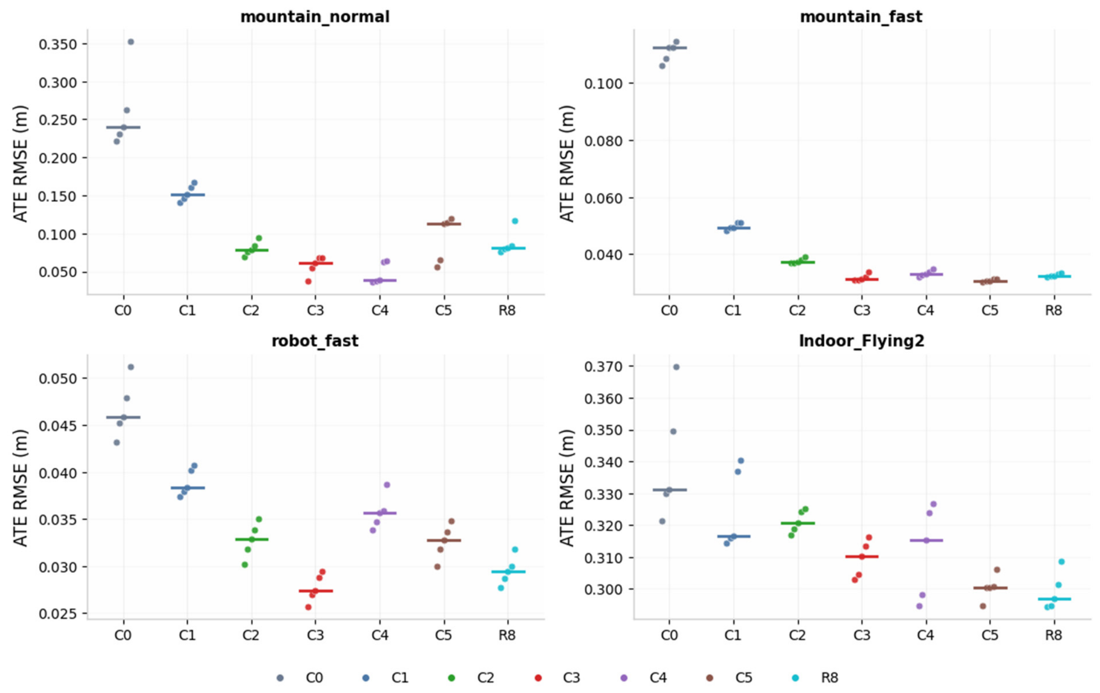
To identify which component produces the gain, we ablate one component at a time on the identical system. On mountain_fast, the median ATE descends from 0.1123 m with the conventional module to 0.0495 m with the lowered trigger operating point, 0.0374 m with temporal-consistency voting added, and 0.0313 m with quality-weighted verification. On robot_fast, it descends from 0.0459 m through 0.0383 m and 0.0328 m to 0.0274 m, and on mountain_normal from 0.2398 m through 0.1516 m and 0.0779 m to 0.0607 m. The conventional module degrades accuracy relative to loop closure disabled on mountain_fast because it accepts false loops under repetitive visual patterns, while the proposed components remove those errors. On mountain_normal, the fallback and the count-based bypass never fire, so C3, C4, and C5 are algorithmically identical there; their different medians and the overall run range of 0.036657–0.119857 m therefore reflect run-to-run variability rather than component effects. On Indoor_Flying2, the medians of C1–C5 and R8 range from 0.2968 m to 0.3207 m, compared with 0.3310 m for C0, showing that the component effects are more sequence-dependent. Removing the fallback degrades robot_fast from 0.0274 m to 0.0357 m, where temporal support is thin. The results are listed in Table 3 and Figure 11.
Table 3.
Component-wise ablation of the loop module on four sequences. Each entry is the median of five runs; Figure A1 visualizes all individual runs.
Figure 11.
Component-wise ablation ATE by sequence; each bar is the median of five runs, and lower is better.
Each configuration was run five times under identical conditions on each of the four ablation sequences. Table 3 reports the third value of each sorted five-run set, and Figure A1 visualizes every individual run. On mountain_normal, the medians 0.0381 m (C4), 0.0607 m (C3), and 0.1124 m (C5) come from disjoint five-run sets rather than three measurements of one shared run. Repeating a four-decimal median across Table 2 and Table 3, and subsequent 11 sequence test tables denotes reuse of the same reported median for the same configuration; repetition across C3, C4, and C5 reflects different median runs of algorithmically identical settings on that sequence. The full-configuration five-run spreads are 30.4, 2.8, 3.8, and 13.2 mm on mountain_normal, mountain_fast, robot_fast, and Indoor_Flying2, respectively.
Figure A1 shows the C2 and C3 run distributions rather than comparing a median step with only one spread. The C2 ranges are 0.069318–0.094307, 0.036917–0.038977, 0.030141–0.034966 and 0.316952–0.325222 m, and the C3 ranges are 0.038068–0.068516, 0.030915–0.033707, 0.025684–0.029472 and 0.303084–0.316300 m on mountain_normal, mountain_fast, robot_fast and Indoor_Flying2, respectively. The median C2-to-C3 reductions are 0.0172, 0.0061, 0.0054, and 0.0106 m. Every C3 run is below every C2 run on all four sequences, with between-distribution gaps of 0.000802, 0.003210, 0.000669, and 0.000652 m. With five runs per configuration, this is consistent distributional evidence, not a significance test. On mountain_normal, the broader variation among the algorithmically equivalent C3, C4, and C5 settings still cautions against attributing the entire median difference to quality-weighted verification alone.
The configurations listed in Table 3 are defined as follows. C0 is the conventional loop module with the inherited fixed 0.05 trigger and 0.015 candidate threshold, without temporal-consistency voting and with raw-inlier verification. C1 changes only the trigger to the online-computed scoring trigger. Since Section 3.1 shows that its decisions coincide with the fixed 0.03 lower bound on these sequences, C1 measures the effect of lowering the trigger operating point from 0.05 to 0.03, not the effect of changing trigger decisions between queries. C2 adds temporal-consistency voting and the temporal fallback while retaining raw-inlier verification. C3 is the full system and adds match-quality-weighted verification with the dual acceptance condition. C4 is C3 without the temporal fallback, so queries without temporal support are dropped instead of falling back to the highest current score. C5 is C3 with the count-based strong-inlier bypass disabled by setting mqwv_strong_inliers = 1,000,000, so every candidate must satisfy the quality channel. R8 retains the full C3 pipeline but restores the inherited fixed 0.05 trigger and 0.015 candidate threshold as a fixed-threshold control.
We further evaluated retrieval depths of 2, 4, 8, and 12. Increasing depth from 4 to 12 raises verified candidates from 69 to 138 on robot_fast and from 100 to 121 on Indoor_Flying2, and accepted loops from 9 to 16 and from 77 to 87, respectively. These additional accepted loops do not produce a monotonic ATE reduction. Relative to depth 4, the ATE values at depths 8 and 12 remain within 5 mm on mountain_fast, robot_fast, and Indoor_Flying2, whereas depth 2 degrades accuracy, for example from 0.0313 m at depth 4 to 0.0384 m on mountain_fast. On mountain_normal, the ATE ranges from 0.0607 m to 0.0797 m across depths, with 133 to 142 accepted loops and no monotonic trend. The trigger rejection rate on robot_fast remains near 39% for all depths, and the mean query time remains similar, for example, 3.24–3.44 ms on mountain_normal. Candidates from ranks five and beyond are admitted frequently, entering 341 of 344 queries on mountain_normal at depth 8, but the measured outcome is reported directly as ATE rather than as a claim that recall saturates. A possible explanation is that correct loops concentrate in the top ranks and that deeper candidates pass verification mainly where the trajectory is already well constrained; however, the locations of the additional loops were not recorded, so this explanation remains a hypothesis. Depth four is retained as the operating point. The results are listed in Table 4 and Figure 12.
Table 4.
Retrieval-depth sensitivity on four sequences.
Figure 12.
Retrieval-depth sensitivity of ATE by sequence.
Figure 13 compares ATE heat maps on mountain_normal with loop closure enabled and disabled. The results support combining the lowered trigger operating point, per-query candidate gate, temporal-consistency voting, and MQWV to suppress cumulative drift while retaining positive gains on the tested short sequences with mild drift.
Figure 13.
ATE heat maps on mountain_normal: (a) with loop closure enabled; (b) with loop closure disabled.
The loop-module ablation alone does not fully demonstrate system-level performance. The next section therefore compares MEVFusion-LD with the three event-based multimodal localization systems introduced above.
6.2. MEVFusion-LD Positioning-Accuracy Comparison Experiment
To validate the performance of the proposed loop-closure algorithm, this section compares its positioning accuracy with PL-EVIO, ESIO, and ESVIO on 11 sequences. The results are shown in Table 5 and Figure 14. MEVFusion-LD outperforms loop-enabled ESVIO on all 11 sequences, with an average per-sequence ATE reduction of 26.8%, and achieves the best accuracy among the four methods on 9 of them.
Table 5.
ATE comparison on 11 sequences.
Figure 14.
Positioning-accuracy comparison.
Across all sequences, MEVFusion-LD reduces the mean ATE from 0.1329 m for ESVIO to 0.0933 m, a 29.8% reduction on a mean-of-ATEs basis that complements the 26.8% average per-sequence reduction. It also reduces mean ATE by 41.1% relative to ESIO (0.1584 m) and by 50.0% relative to PL-EVIO (0.1865 m). Baseline rankings vary substantially across sequences: ESIO performs well on mountain_fast but poorly on desk_normal, whereas MEVFusion-LD remains among the top two methods on every sequence, indicating stronger scene adaptability.
The largest improvement occurs on mountain_normal. ESVIO reaches an RMSE of 0.3595 m, exceeding the loop-disabled result of 0.3362 m and indicating that its loop module introduced numerous erroneous constraints. MEVFusion-LD reduces RMSE to 0.0607 m—81.9% below the loop-disabled result and 83.1%, 81.7%, and 82.8% below ESVIO (0.3595 m), ESIO (0.3322 m), and PL-EVIO (0.3522 m), respectively. The mountain scene contains multiple calibration plates with highly self-similar textures and a wide field of view. BoW scores are generally high across positions, so fixed-threshold retrieval produces many false candidates that raw-inlier verification can accept. Pose-graph optimization then propagates these erroneous loop edges throughout the trajectory.
MEVFusion-LD uses AST to adjust the candidate threshold and MQWV to reject false positives through the weighted inlier ratio, preserving high-quality genuine loops and substantially improving accuracy. ESVIO also performs worse than loop-disabled operation on mountain_fast, further demonstrating the limitations of fixed-threshold loop closure.
Only on robot_normal is PL-EVIO slightly superior to MEVFusion-LD. This is a slow, regular indoor sequence with distinctive visual features and abundant genuine loop opportunities. All methods can obtain correct constraints, so the benefit of improving the loop-decision mechanism is limited. MEVFusion-LD nevertheless improves ATE by 50.1% relative to ESVIO and remains close to the best baseline. In contrast, although PL-EVIO is best on this sequence, it degrades on desk_normal, mountain_normal, and all MVSEC sequences.
To compare stability under identical hardware, front-end, and backend configurations, Figure 15 and Figure 16 show ATE heat maps and error distributions for ESVIO and MEVFusion-LD on hdr_normal. The ESVIO trajectory contains extensive orange-red high-error regions near its end, whereas the MEVFusion-LD trajectory remains almost entirely within the dark-blue low-error range, with maximum ATE reduced to 0.070 m. These results illustrate the proposed method’s adaptability to high-dynamic-range illumination.
Figure 15.
ATE heat maps on hdr_normal: (a) with loop closure disabled; (b) with loop closure enabled.
Figure 16.
Comparison of trajectory error distributions on the hdr_normal sequence: (a) ESVIO; (b) MEVFusion-LD.
Overall, MEVFusion-LD outperforms loop-enabled ESVIO on all 11 sequences and achieves the best accuracy among the four methods on 9 sequences, demonstrating the effectiveness of combining AST, temporal-consistency voting, and MQWV across diverse scenarios.
6.3. Performance Analysis of MEVFusion-LD Loop Detection
This section quantitatively analyzes retrieval triggering, candidate screening, and geometric verification. Table 6 and Figure 17 summarize pipeline statistics, Table 7 reports internal sequence-level indicators, and Figure 18 relates the computed trigger threshold to the BoW score level. Accuracy attribution is established directly through the component-wise ablation and fixed-threshold control in Section 6.1.
Table 6.
Statistics of the loop-detection pipeline on all test sequences, including the mean trigger threshold () and the mean candidate threshold ().
Figure 17.
Loop candidate screening and geometric-verification statistics.
Table 7.
Internal statistics of the loop-detection algorithm: mean nearest-neighbor score (), mean trigger threshold (), mean temporal-consistency score (), and mean weighted inlier ratio ().
Figure 18.
Sequence-level mean nearest-neighbor BoW score versus mean computed trigger threshold. The dashed line marks the inherited fixed 0.05 trigger threshold.
All measurements were run on a 13th Gen Intel Core i7-13650HX processor with 14 cores and 20 threads at a 2.60 GHz base clock, 24 GB of memory, and the GPU was not used by the loop module. A complete verified query costs retrieval, descriptor matching, and PnP together, with means of 0.56–3.31 ms, 0.42–5.42 ms, and 1.68–3.28 ms per stage across sequences, and the worst observed PnP took 5.7 ms. Optimization runs on a separate thread with a mean of 6.2–18.5 ms and a worst pass of 25.8 ms; the backlog never exceeded 14 keyframes and drained without blocking the front-end. The iteration count reported by the solver includes the initial evaluation, so six recorded iterations correspond to the configured limit of five steps. The reported passes on mountain_normal, mountain_fast and robot_fast record three to five iterations with the convergence flag, whereas all nine passes on Indoor_Flying2 record six with a non-converged termination flag. The accepted loop set is fixed upstream by verification, and every accepted loop re-optimizes the whole graph from the current state. Each capped Indoor_Flying2 pass reduced the solver cost by 24% to 49%, but this cost decrease is not evidence of convergence or of recovery of final accuracy. No larger-cap comparison was performed, so the effect of the iteration cap on final accuracy was not evaluated; the reported Indoor_Flying2 result is obtained entirely with these capped, non-converged passes.
For the four evaluation sequences, the triggered candidates count the queries that pass the trigger over the full run of the same logged run analyzed in Table 8 and Table 9, and the two threshold means are averaged over the post-warm-up queries with retrieval results, the population of Table 9.
Table 8.
Stage-wise candidate funnel of the full configuration on four sequences, where each selected query verifies exactly one candidate pair.
Table 9.
AST threshold behavior and unweighted inlier ratios by sequence.
As shown in Table 6 and Figure 17, the geometric-verification pass rate is strongly scene-dependent. On mountain_fast, which has a wide field of view and repetitive visual patterns, most triggered candidates are false: 375 queries trigger candidates over the full logged run, but only 3 loops are accepted, giving a pass rate of 0.8%. On mountain_normal, 389 queries trigger candidates and 137 loops are accepted, giving 35.2%. The mean weighted inlier ratio of the accepted mountain_normal loops is 0.3167, indicating limited match support even after verification. ESVIO accuracy also decreases on both mountain sequences because of erroneous loop constraints. Its RMSE of 0.0477 m on mountain_fast is 35.5% worse than the 0.0352 m loop-disabled result, and its RMSE of 0.3595 m on mountain_normal is worse than the 0.3362 m loop-disabled result. MEVFusion-LD reduces ATE by 34.4% and 83.1% relative to ESVIO on these two sequences, respectively. For the fast-motion sequences, the pass rates are 6.7% on robot_fast, 11.7% on hdr_fast, and 22.4% on desk_fast.
These pass rates describe verification acceptance, not detection recall. In particular, the ground-truth-labeled analysis on mountain_fast below gives 100% precision among the three accepted pairs but only 4.4% verification-stage recall, so the low acceptance rate must not be interpreted as high overall detection accuracy.
In regular scenarios, where genuine loop opportunities are more abundant, the pass rate ranges from 68.3% to 85.4%. The trigger-threshold means depend on the averaging population. Table 7 averages all logged detection queries, including the warm-up segment where the trigger rests at its 0.05 default, and ranges from 0.0380 on desk_fast to 0.2243 on mountain_normal. Table 6 instead averages post-warm-up queries with retrieval results and gives 0.250 on mountain_normal, where every such query is at the upper bound, as Table 9 shows. The values 0.2243 and 0.250 therefore describe different query populations and are not conflicting. As Section 3.1 shows, this threshold movement does not change trigger decisions; the scene-dependent score level instead affects the candidate gate. The mean BoW query time ranges from 0.56 to 3.45 ms, and the measured loop-detection cost remains below the keyframe-generation interval, meeting the online-operation requirement on the tested sequences.
Figure 18 plots the sequence-level all-log means reported in Table 7. The mean computed trigger threshold is 0.0390 on robot_fast, 0.0517 on Indoor_Flying2, 0.1750 on mountain_fast, and 0.2243 on mountain_normal. The corresponding post-warm-up means in Table 6 are 0.036, 0.052, 0.196, and 0.250; they differ because the warm-up queries at the 0.05 default are excluded. The mean candidate threshold remains near its upper bound on all sequences, with the lowest post-warm-up mean of 0.023 on robot_fast, and its per-query movement is quantified in Table 9.
The two effects of the scoring scheme are separated explicitly. Lowering the operating point: comparing fixed-threshold control R8, which restores the inherited 0.05 trigger and 0.015 candidate threshold, with C3 gives 0.0810 m to 0.0607 m on mountain_normal, 0.0326 m to 0.0313 m on mountain_fast, and 0.0294 m to 0.0274 m on robot_fast. On Indoor_Flying2, the same change degrades the median from 0.2968 m to 0.3101 m, so the benefit of the lower operating point is scene-dependent rather than universal. Changing the threshold between queries: for the trigger, this effect is exactly zero, since its decisions coincide with the fixed 0.03 bound in all 1380 post-warm-up queries. For the candidate gate, fixing it at its 0.030 upper bound and replaying the logged queries leaves the admitted candidate set unchanged on mountain_normal, mountain_fast and Indoor_Flying2, and admits 69 additional pairs across 61 of 219 queries on robot_fast. Nine affected queries forward a candidate to verification, and one such query also accepts its top-ranked candidate; however, no movement-admitted extra pair is accepted. Consequently, no accepted loop is attributed to per-query candidate-gate movement, and the accuracy differences are discussed in terms of the lowered operating range and the downstream temporal and geometric modules rather than trigger adaptation.
Each point in Figure 18 represents one sequence: the horizontal coordinate is the mean nearest-neighbor BoW score over all logged detection queries, and the vertical coordinate is the mean computed trigger threshold over the same queries. The points show a broad positive association, but not a strictly monotonic ordering; sequences with similar mean scores can have different mean thresholds because the per-query score means and standard deviations vary before averaging. The dashed line marks the inherited fixed 0.05 threshold for visual reference. Independently of this sequence-level trend, Section 3.1 shows that the trigger decisions are identical to the fixed 0.03 lower bound on the evaluated queries.
Table 7 also reports the mean weighted inlier ratio of accepted loops. The values are high on desk_normal and Indoor_Flying3, whereas mountain_fast and mountain_normal give 0.3320 and 0.3167, respectively. Together with their low acceptance rates, this indicates that accepted loops in the mountain sequences have limited match support even after verification. The ground-truth analysis below therefore distinguishes verification precision from recall rather than treating pass rate alone as detection quality.
The mean temporal-consistency score further characterizes the voting mechanism. The is substantially higher for high-dynamic-range or repetitive-texture sequences, including hdr and mountain, than for sequences with more distinctive features, including robot, desk, and Indoor_Flying. Thus, when scores are densely distributed and candidates trigger frequently, candidate decisions rely more on multiframe voting within the sliding window than on individual retrieval scores, reducing sensitivity to isolated score fluctuations.
Candidate correctness is established against ground truth, where a pair is counted as a genuine loop opportunity when the viewpoints lie within 0.3 m and 30 degrees, the envelope inside which the uncompensated descriptors still assemble 15 inliers. On mountain_fast, of the 322 verified candidates, 42 were rejected before PnP, 274 by the dual condition, and 3 by the pose gate, leaving 3 accepted loops, all genuine with ground-truth separation within 0.20 m and 11 degrees. Among the labeled rejections, 79.8% lie outside the covisibility envelope and are correctly rejected, while 20.2% are valid opportunities conservatively discarded. Under this labeling, 322 candidate pairs were evaluated: the three accepted pairs are all genuine, giving a precision of 100%, and 65 of the 319 rejected pairs are genuine opportunities, giving a verification-stage recall of 4.4% on this sequence. This low recall is the precision-first trade-off of the verification stage and must accompany any interpretation of the acceptance rate as detection performance. The 34.4% ATE reduction on mountain_fast is attributed using the component-wise ablation in Table 3 rather than the candidate count or pass rate alone.
The detection log is flushed before the final frames of each run, so the verification log additionally covers 1, 32, 1 and 1 trailing queries on mountain_normal, mountain_fast, robot_fast and Indoor_Flying2, respectively. These queries lie outside the common interval of Table 8, and all are rejected at some verification stage, so the accepted counts equal the full-run totals. Every selected query verifies exactly one candidate pair, and the selected and verified counts are therefore identical by construction. The visualization of Table 8 is shown in Figure 19.
Figure 19.
Stage-wise candidate funnel by sequence.
Table 9 summarizes the behavior of the two computed thresholds on the four evaluation sequences. The trigger threshold is computed online as μ + 0.35σ and clamped to the interval 0.03 to 0.25, and the candidate threshold τo is computed as μ + 0.04σ and clamped to the interval 0.012 to 0.030. All shares use post-warm-up queries with retrieval results as denominators: 339, 307, 219, and 515, respectively. Every rejected query sits in the lower-bound group of the trigger, since the trigger passes whenever the highest score exceeds 0.03. On mountain_fast, seven of the nine lower-bound queries are rejected, which is exactly the reported 2.3%, and on robot_fast, 85 of the 129 lower-bound queries are rejected, giving 38.8%. The candidate threshold saturates at its upper bound in 100%, 96.1%, 33.8%, and 88.2% of queries on mountain_normal, mountain_fast, robot_fast, and Indoor_Flying2, respectively.
The two thresholds play different roles. Trigger decisions are equivalent to the lower bound, as shown in Section 3.1, whereas the candidate threshold moves below 0.030 in 66.2% of queries on robot_fast, 11.8% on Indoor_Flying2, and 3.9% on mountain_fast, and never on mountain_normal. Counting candidate pairs whose scores lie between the computed candidate threshold and 0.030, per-query movement admits 69 additional pairs across 61 queries on robot_fast and none on the other sequences. Nine affected queries forward candidates to verification: eight are rejected, and frame 237 accepts its already-admitted top-ranked candidate rather than a movement-admitted extra. Therefore, 0 of the 69 additional pairs become accepted loops and 0 become accepted ground-truth-genuine loops. All nine accepted robot_fast loops enter as top-scoring candidates. The additional pairs’ isolated contribution to trajectory accuracy is therefore unavailable; the robot_fast gain is attributed jointly to the lowered trigger operating point, temporal-consistency voting over the enlarged candidate pool, and quality-weighted verification, rather than to a demonstrated benefit from the 69 extra pairs. Independently of per-query movement, the lower operating range admits 46, 179, and 235 additional candidate scores in the 0.03–0.05 band on mountain_fast, robot_fast, and Indoor_Flying2, respectively.
Figure 20 visualizes the same statistics. On mountain_normal, the computed trigger threshold saturates at its upper bound in every query because high scores push the unclamped value beyond 0.25. On robot_fast, globally weak scores pin 58.9% of the thresholds at the lower bound, where 38.8% of all queries are rejected. On mountain_fast and Indoor_Flying2, the threshold lies inside the clamping interval in 55.0% and 99.4% of queries, respectively. Its numerical value varies with query-score statistics even though Section 3.1 shows that its decisions remain equivalent to the fixed 0.03 lower bound. On mountain_fast, robot_fast and Indoor_Flying2, the candidate threshold τo saturates at its upper bound more often than the trigger threshold, confirming that the tight candidate bound filters the retrieval tail while the trigger governs activation.
Figure 20.
Computed-threshold behavior: share of queries by sequence.
Table 10 and Figure 21 present the per-stage timing breakdown. Summing retrieval, descriptor matching, and PnP, a complete verified query costs 12.01 ms on mountain_normal, 5.18 ms on mountain_fast, 2.66 ms on robot_fast, and 9.98 ms on Indoor_Flying2—well below the keyframe period on every sequence. Descriptor matching scales with texture richness, from 0.42 ms on robot_fast to 5.42 ms on mountain_normal, while PnP requires 1.68–3.28 ms with a worst observed pass of 5.7 ms. Pose-graph optimization runs on a separate thread and dominates the budget on Indoor_Flying2 at 18.52 ms per pass. Nevertheless, the backlog never exceeds 14 keyframes and drains without blocking the front-end, supporting online operation on all tested sequences.
Table 10.
Loop module timing breakdown.
Figure 21.
Loop module timing breakdown, mean milliseconds per stage.
7. Conclusions
MEVFusion-LD addresses three limitations of loop detection in MEMS-based event-based visual–inertial systems: poor scene adaptability of fixed scoring thresholds, insufficient temporal constraints on candidate decisions, and inability of geometric verification to distinguish match quality. The method combines adaptive scoring, temporal-consistency voting, match-quality weighting, and 4-DoF pose-graph optimization for online trajectory-drift correction.
Experimental results show accuracy gains on all 11 test sequences, with the loop module reducing ATE by 52.8% on average and by up to 81.9%. Compared with loop-enabled PL-EVIO, ESIO, and ESVIO, MEVFusion-LD outperforms ESVIO under the same hardware configuration on every sequence and reduces mean ATE by 29.8%. It achieves the best accuracy on 9 sequences, and its millisecond-level query time supports online operation.
Because mainstream EVIO benchmarks use MEMS-grade inertial sensors, and MEMS sensors dominate mass-, volume-, and power-constrained platforms such as drones, CubeSats, and space robots, the proposed adaptive loop-closure framework is relevant to resource-constrained platforms requiring long-term operation without external positioning. Future work will evaluate event-vision datasets and experimental facilities designed for space applications and investigate coupling between MEMS gyroscope error states and loop constraints within a unified estimation framework.
Author Contributions
Conceptualization, H.Y.; validation, H.Y.; formal analysis, H.Y.; data curation, H.Y.; resources, J.Z.; project administration, J.Z.; funding acquisition, J.Z.; software, Z.Z.; visualization, Y.L.; supervision, K.Z.; writing—review and editing, F.Z. and Q.Z. All authors have read and agreed to the published version of the manuscript.
Funding
This work was supported in part by the National Natural Science Foundation of China under Grant 62305393, and in part by the Innovation Capability Support Program-Science and Technology Innovation Team Project 2025RS-CXTD-046.
Institutional Review Board Statement
Not applicable.
Informed Consent Statement
Not applicable.
Data Availability Statement
The data and code related to this study are available from the corresponding author upon reasonable request.
Conflicts of Interest
The authors declare no conflicts of interest.
Appendix A
This appendix visualizes the five individual runs underlying every median reported in Table 3. For each configuration and sequence, the third value of the sorted five-run set equals the corresponding Table 3 median after rounding to four decimals. On mountain_normal, C3, C4, and C5 are algorithmically identical because the fallback and count-based bypass never fire. Their medians of 0.0607, 0.0381, and 0.1124 m therefore come from different runs of equivalent settings and quantify run-to-run variation rather than three distinct component effects.
Figure A1 shows every run of each configuration. On all four sequences, every C3 run is below every C2 run. This consistent ordering supports the reported C2-to-C3 improvement as a distributional observation over five runs, but it is not a significance test; on mountain_normal, the variation among equivalent C3, C4, and C5 settings remains a reason not to attribute the entire difference to a single component.
Figure A1.
Distribution of the five runs of each configuration on the four evaluation sequences, with horizontal lines marking medians. C2 is shown in green and C3 in red.
References
- Yazdi, N.; Ayazi, F.; Najafi, K. Micromachined inertial sensors. Proc. IEEE 1998, 86, 1640–1659. [Google Scholar] [CrossRef] [Scilit]
- Passaro, V.M.N.; Cuccovillo, A.; Vaiani, L.; De Carlo, M.; Campanella, C.E. Gyroscope technology and applications: A review in the industrial perspective. Sensors 2017, 17, 2284. [Google Scholar] [CrossRef] [Scilit] [PubMed]
- Nguyen, M.N.; Ha, N.S.; Nguyen, L.Q.; Chu, H.M.; Vu, H.N. Z-axis micromachined tuning fork gyroscope with low air damping. Micromachines 2017, 8, 42. [Google Scholar] [CrossRef] [Scilit]
- Deppe, O.; Dorner, G.; König, S.; Martin, T.; Voigt, S.; Zimmermann, S. MEMS and FOG technologies for tactical and navigation grade inertial sensors—Recent improvements and comparison. Sensors 2017, 17, 567. [Google Scholar] [CrossRef] [Scilit] [PubMed]
- El-Sheimy, N.; Hou, H.; Niu, X. Analysis and modeling of inertial sensors using Allan variance. IEEE Trans. Instrum. Meas. 2008, 57, 140–149. [Google Scholar] [CrossRef] [Scilit]
- Gallego, G.; Delbrück, T.; Orchard, G.; Bartolozzi, C.; Taba, B.; Censi, A.; Leutenegger, S.; Davison, A.J.; Conradt, J.; Daniilidis, K.; et al. Event-based vision: A survey. IEEE Trans. Pattern Anal. Mach. Intell. 2022, 44, 154–180. [Google Scholar] [CrossRef] [Scilit] [PubMed]
- Cohen, G.; Afshar, S.; Morreale, B.; Bessell, T.; Wabnitz, A.; Rutten, M.; van Schaik, A. Event-based sensing for space situational awareness. J. Astronaut. Sci. 2019, 66, 125–141. [Google Scholar] [CrossRef] [Scilit]
- Afshar, S.; Nicholson, A.P.; van Schaik, A.; Cohen, G. Event-based object detection and tracking for space situational awareness. IEEE Sens. J. 2020, 20, 15117–15132. [Google Scholar] [CrossRef] [Scilit]
- Ralph, N.O.; Joubert, R.; Jolley, M.; Afshar, S.; Cohen, G.; van Schaik, A. Real-time event-based unsupervised feature consolidation and tracking for space situational awareness. Front. Neurosci. 2022, 16, 821157. [Google Scholar] [CrossRef] [Scilit] [PubMed]
- Chin, T.-J.; Bagchi, S.; Eriksson, A.; van Schaik, A. Star tracking using an event camera. In Proceedings of the IEEE/CVF Conference on Computer Vision and Pattern Recognition Workshops (CVPRW), Long Beach, CA, USA, 16–17 June 2019; pp. 1646–1655. [Google Scholar]
- Mahlknecht, F.; Gehrig, D.; Nash, J.; Rockenbauer, F.M.; Morrell, B.; Delaune, J.; Scaramuzza, D. Exploring event camera-based odometry for planetary robots. IEEE Robot. Autom. Lett. 2022, 7, 8651–8658. [Google Scholar] [CrossRef] [Scilit]
- Vidal, A.R.; Rebecq, H.; Horstschaefer, T.; Scaramuzza, D. Ultimate SLAM? Combining events, images, and IMU for robust visual SLAM in HDR and high-speed scenarios. IEEE Robot. Autom. Lett. 2018, 3, 994–1001. [Google Scholar] [CrossRef] [Scilit]
- Gao, L.; Liang, Y.; Yang, J.; Wu, S.; Wang, C.; Chen, J.; Kneip, L. VECtor: A versatile event-centric benchmark for multi-sensor SLAM. IEEE Robot. Autom. Lett. 2022, 7, 8217–8224. [Google Scholar] [CrossRef] [Scilit]
- Zhu, A.Z.; Thakur, D.; Özaslan, T.; Pfrommer, B.; Kumar, V.; Daniilidis, K. The multivehicle stereo event camera dataset: An event camera dataset for 3D perception. IEEE Robot. Autom. Lett. 2018, 3, 2032–2039. [Google Scholar] [CrossRef] [Scilit]
- Guan, W.; Chen, P.; Xie, Y.; Lu, P. PL-EVIO: Robust monocular event-based visual inertial odometry with point and line features. IEEE Trans. Autom. Sci. Eng. 2024, 21, 6277–6293. [Google Scholar] [CrossRef] [Scilit]
- Chen, P.; Guan, W.; Lu, P. ESVIO: Event-based stereo visual inertial odometry. IEEE Robot. Autom. Lett. 2023, 8, 3661–3668. [Google Scholar] [CrossRef] [Scilit]
- Qin, T.; Li, P.; Shen, S. VINS-Mono: A robust and versatile monocular visual-inertial state estimator. IEEE Trans. Robot. 2018, 34, 1004–1020. [Google Scholar] [CrossRef] [Scilit]
- Campos, C.; Elvira, R.; Rodríguez, J.J.G.; Montiel, J.M.M.; Tardós, J.D. ORB-SLAM3: An accurate open-source library for visual, visual-inertial, and multimap SLAM. IEEE Trans. Robot. 2021, 37, 1874–1890. [Google Scholar] [CrossRef] [Scilit]
- Calonder, M.; Lepetit, V.; Strecha, C.; Fua, P. BRIEF: Binary robust independent elementary features. In Proceedings of the European Conference on Computer Vision (ECCV), Heraklion, Greece, 5–11 September 2010; pp. 778–792. [Google Scholar]
- Gálvez-López, D.; Tardós, J.D. Bags of binary words for fast place recognition in image sequences. IEEE Trans. Robot. 2012, 28, 1188–1197. [Google Scholar] [CrossRef] [Scilit]
- Kümmerle, R.; Grisetti, G.; Strasdat, H.; Konolige, K.; Burgard, W. g2o: A general framework for graph optimization. In Proceedings of the IEEE International Conference on Robotics and Automation (ICRA), Shanghai, China, 9–13 May 2011; pp. 3607–3613. [Google Scholar]
- Rosten, E.; Drummond, T. Machine learning for high-speed corner detection. In Proceedings of the European Conference on Computer Vision (ECCV), Graz, Austria, 7–13 May 2006; pp. 430–443. [Google Scholar]
- Robertson, S. Understanding inverse document frequency: On theoretical arguments for IDF. J. Doc. 2004, 60, 503–520. [Google Scholar] [CrossRef] [Scilit]
- Fischler, M.A.; Bolles, R.C. Random sample consensus: A paradigm for model fitting with applications to image analysis and automated cartography. Commun. ACM 1981, 24, 381–395. [Google Scholar]
- Lepetit, V.; Moreno-Noguer, F.; Fua, P. EPnP: An accurate O(n) solution to the PnP problem. Int. J. Comput. Vis. 2009, 81, 155–166. [Google Scholar] [CrossRef] [Scilit]
- Huber, P.J. Robust Statistics; John Wiley & Sons: New York, NY, USA, 1981. [Google Scholar]
- Umeyama, S. Least-squares estimation of transformation parameters between two point patterns. IEEE Trans. Pattern Anal. Mach. Intell. 1991, 13, 376–380. [Google Scholar] [CrossRef] [Scilit]
- Grupp, M. evo: Python Package for the Evaluation of Odometry and SLAM. Available online: https://github.com/MichaelGrupp/evo (accessed on 12 September 2026).
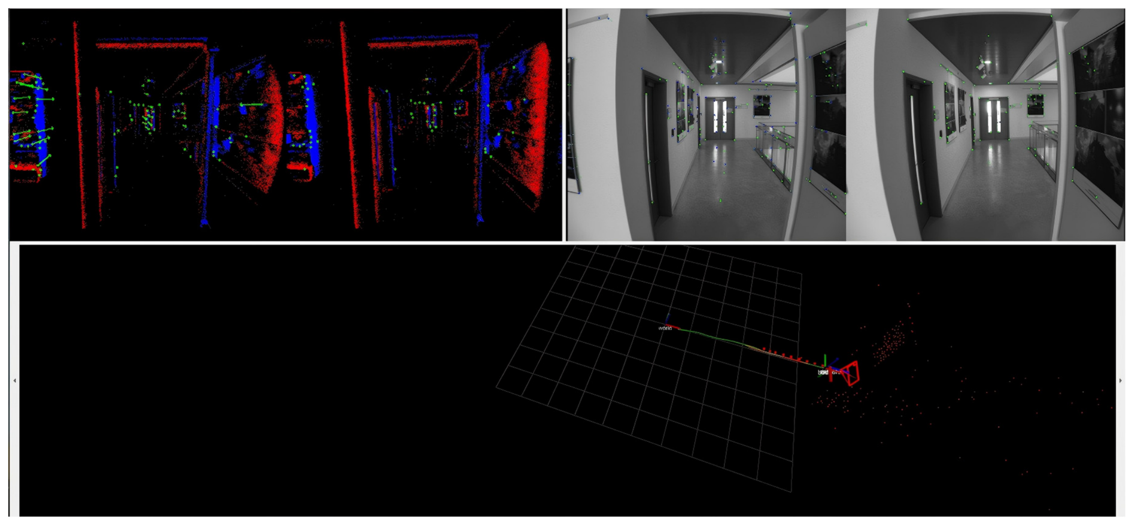
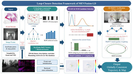
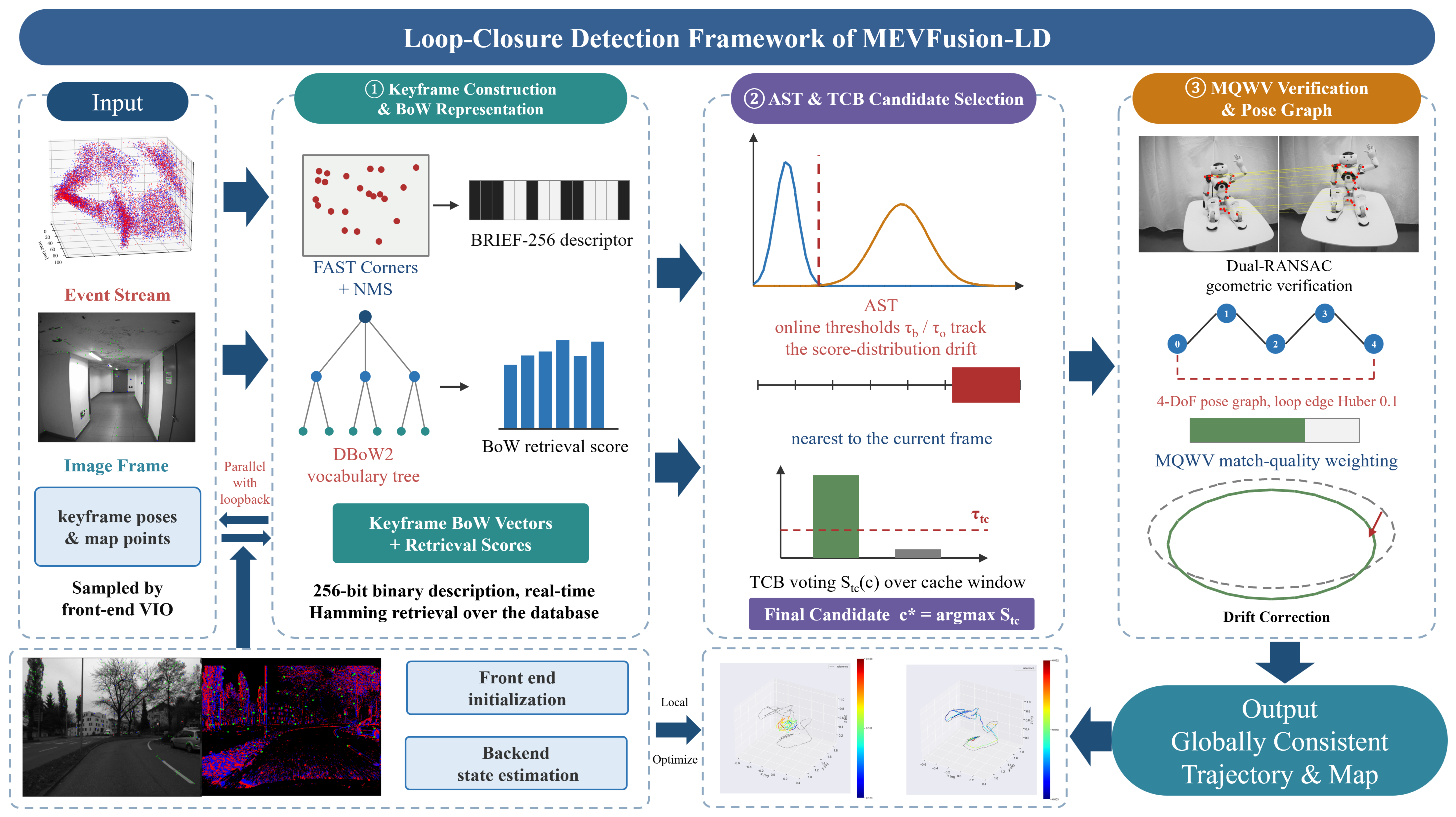
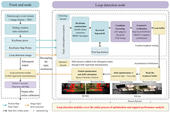
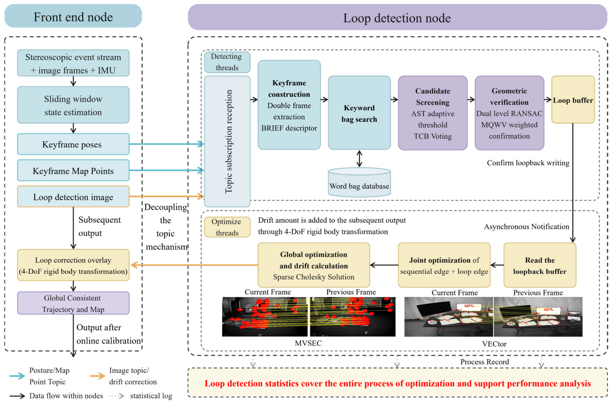
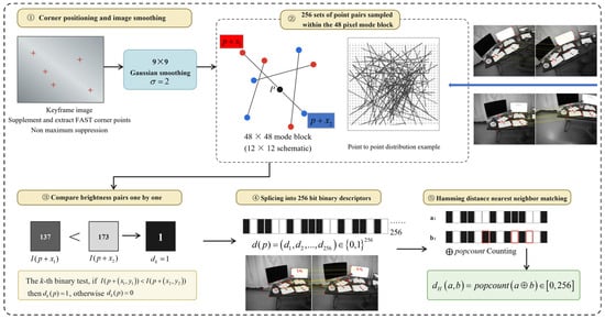
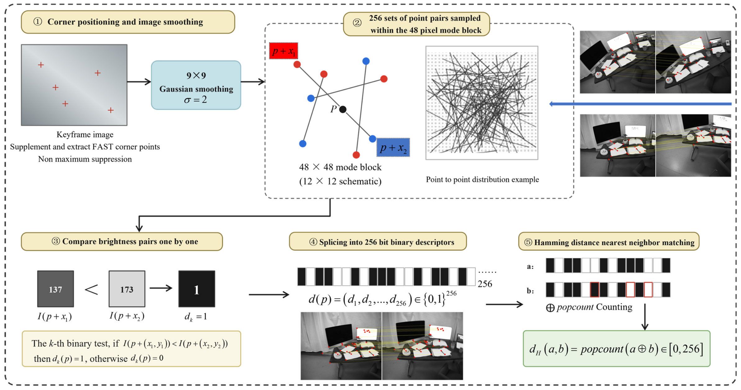
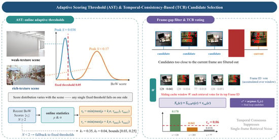
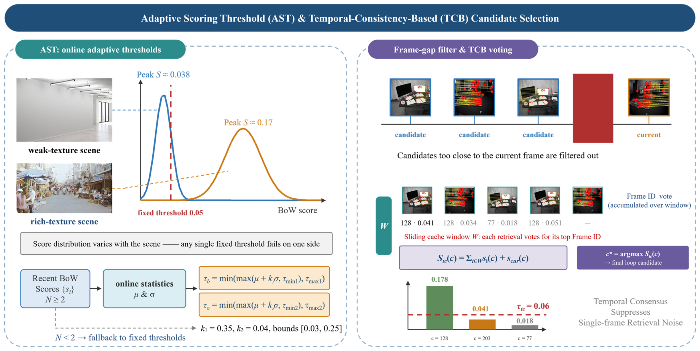
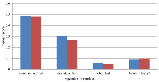
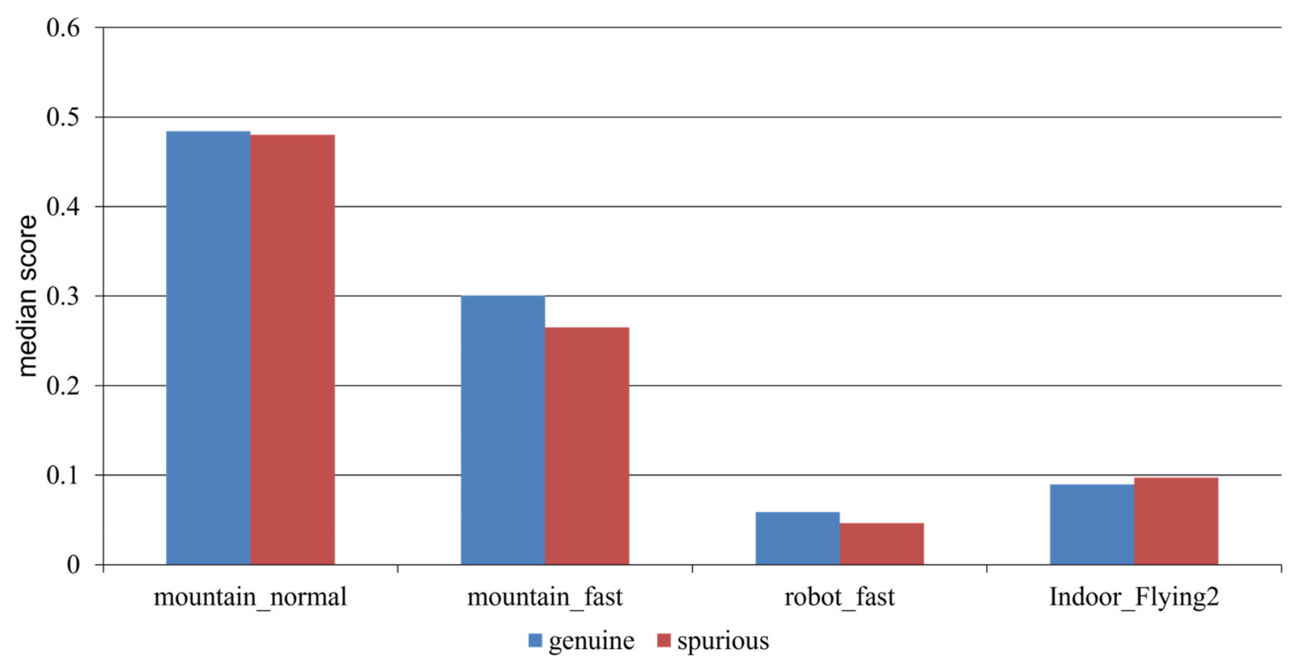
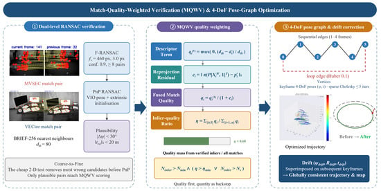
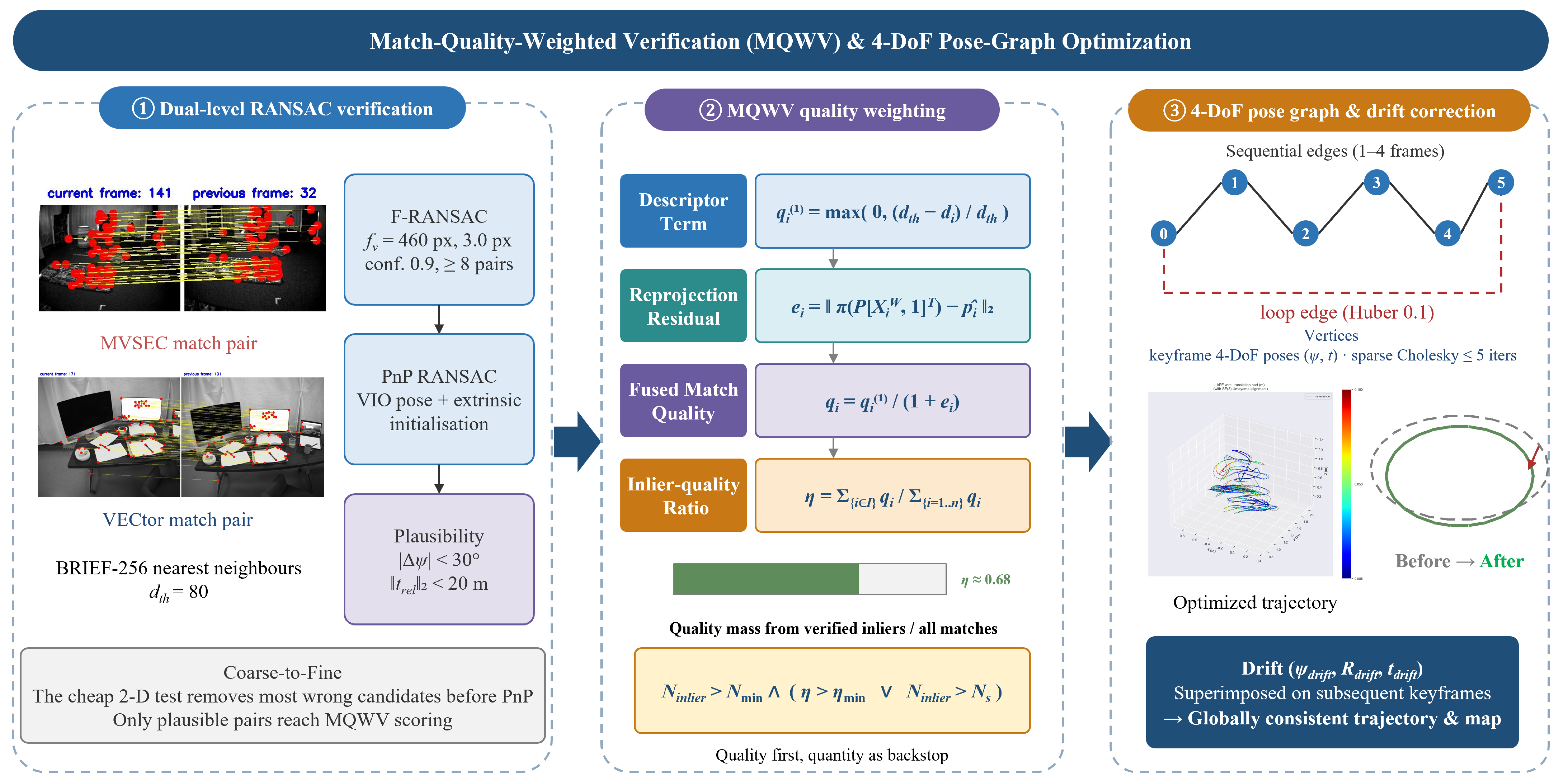
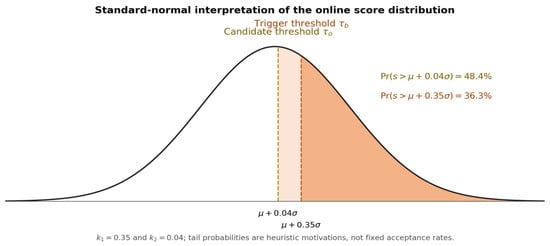
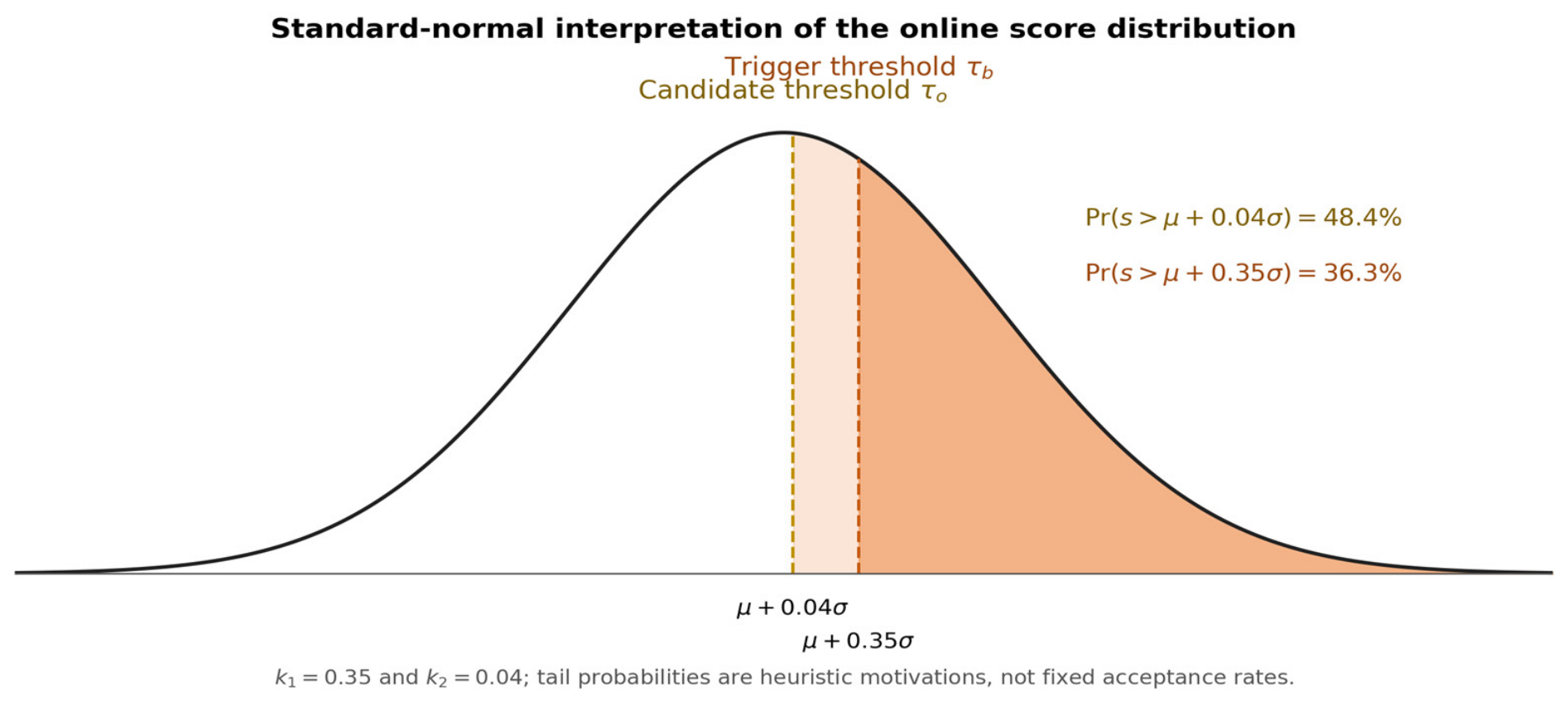
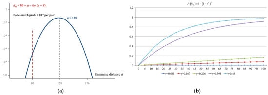
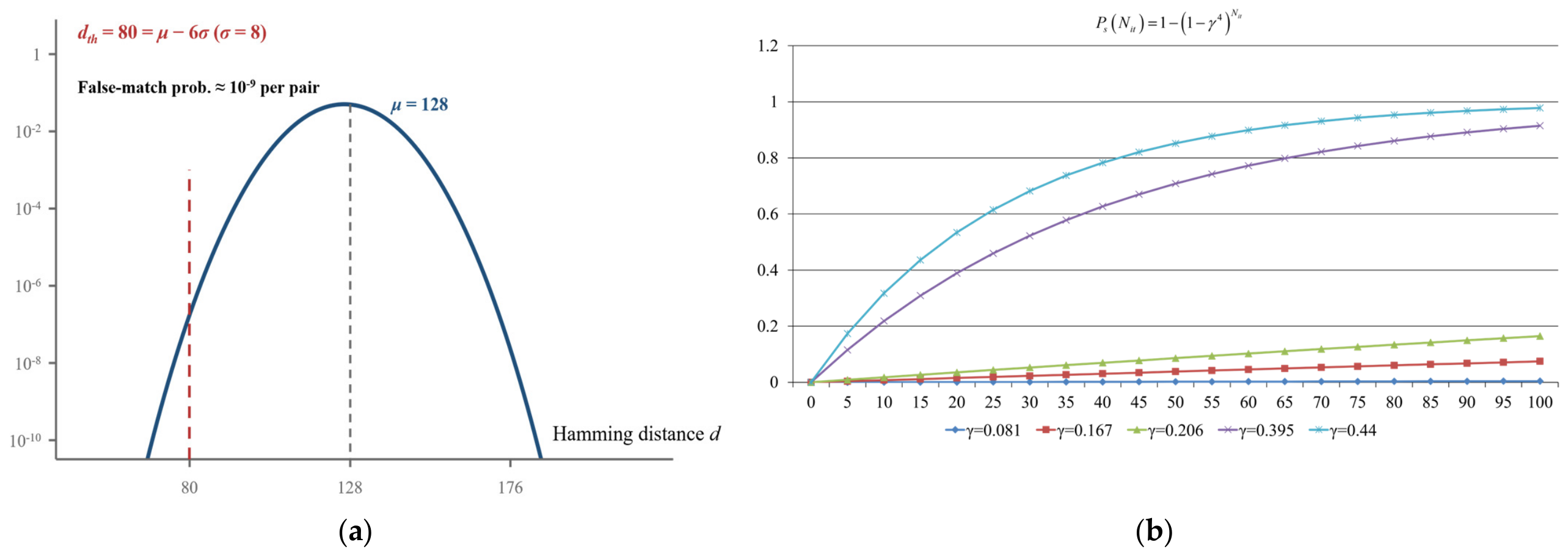
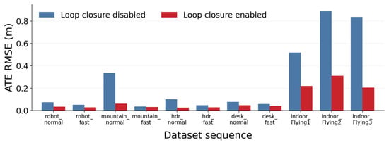
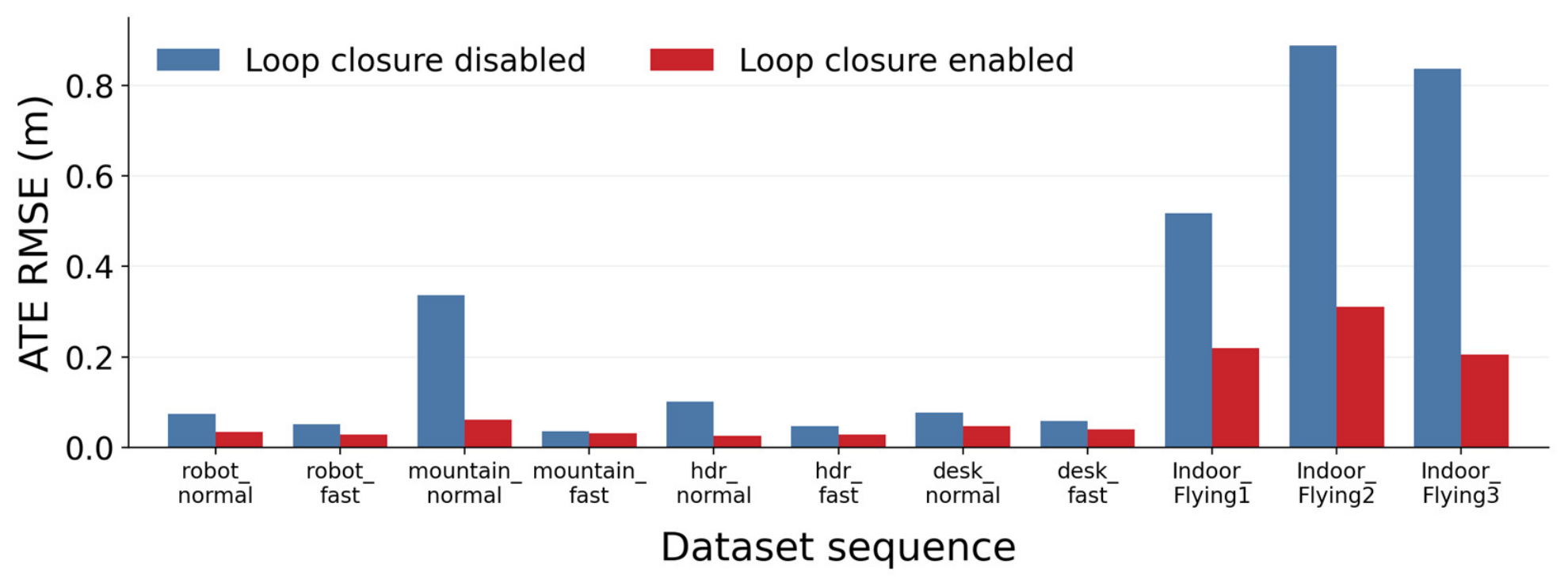
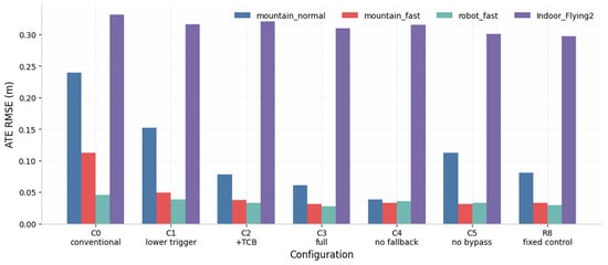
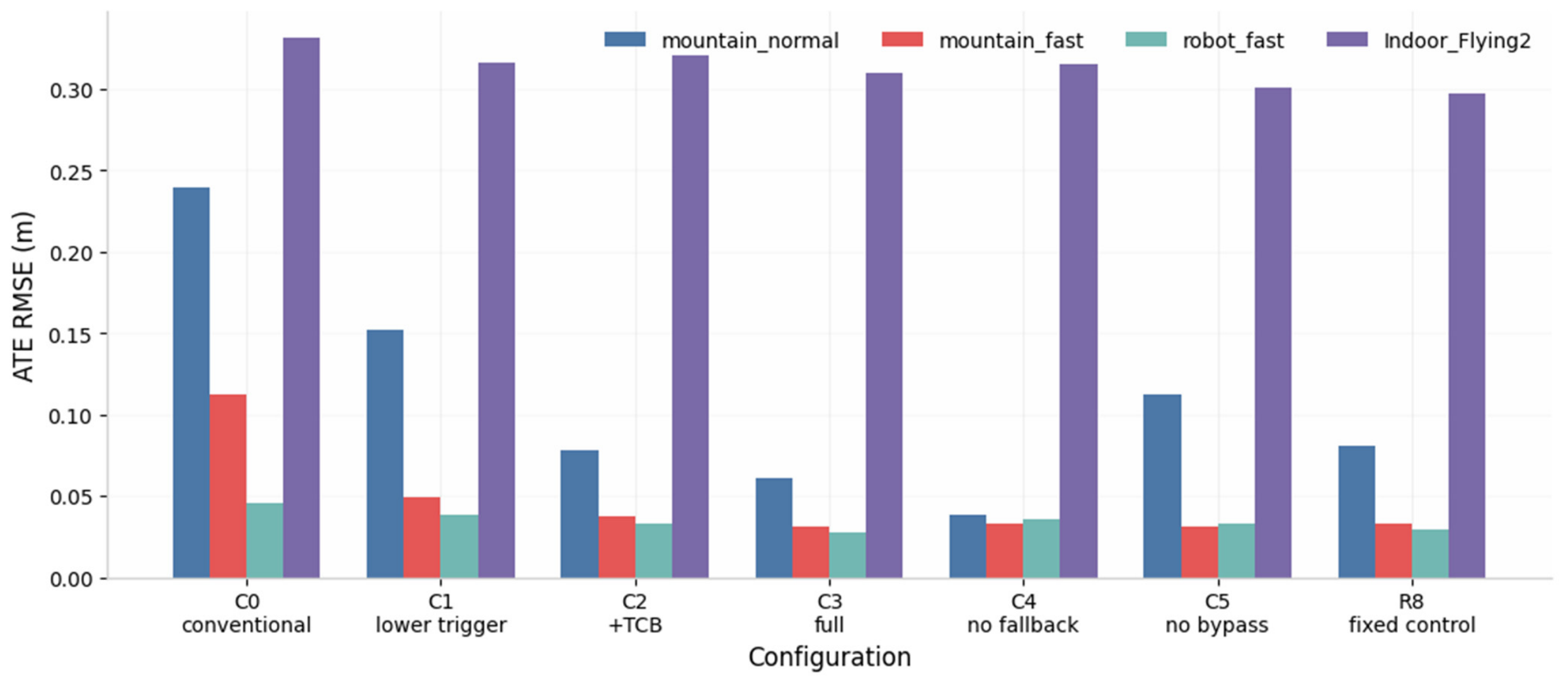
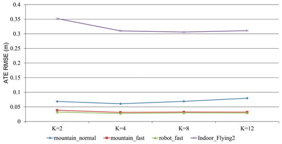
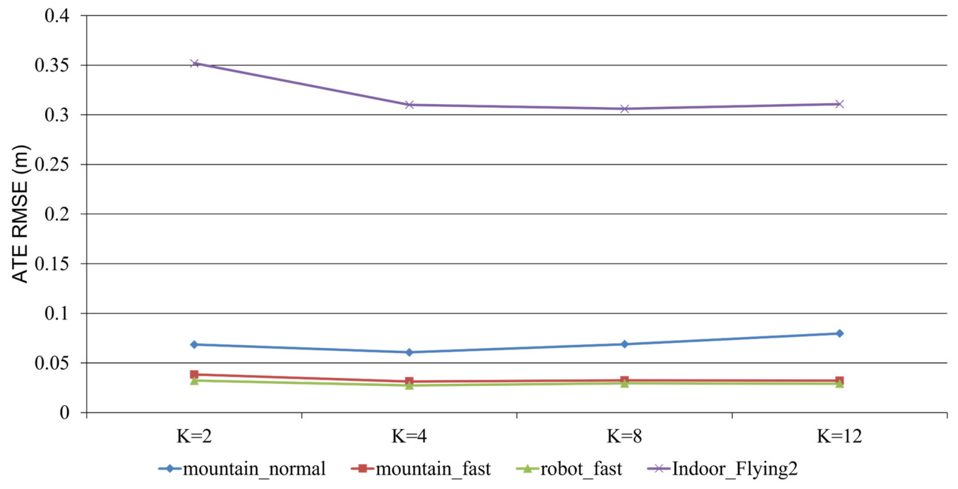
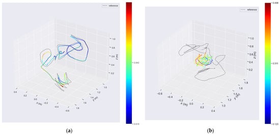
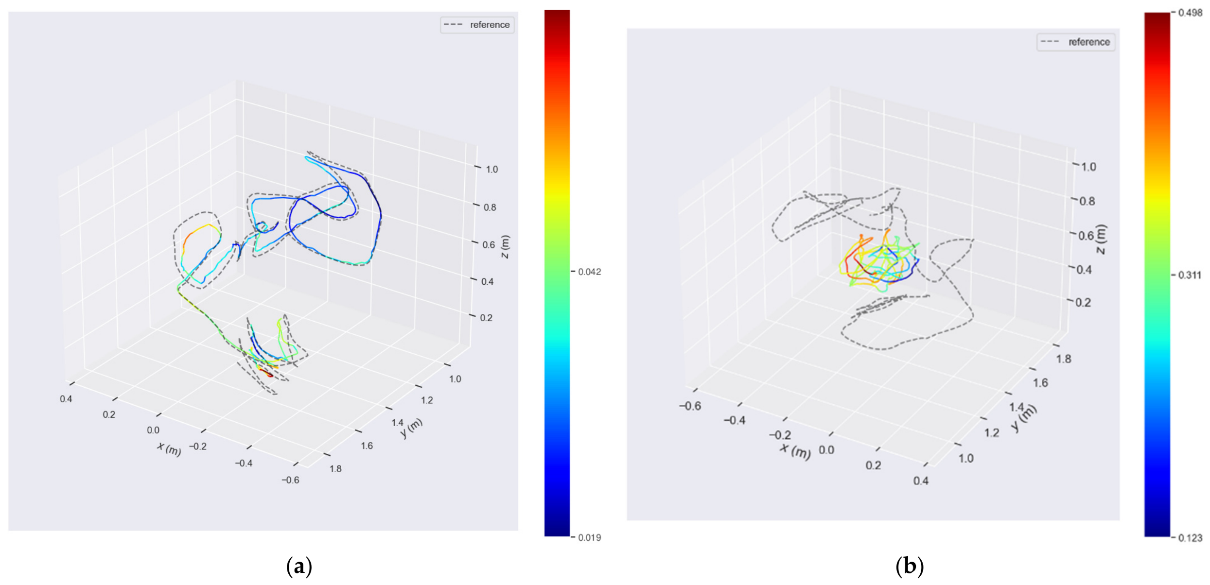
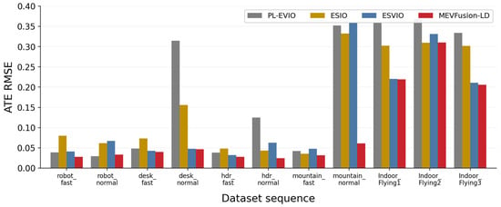
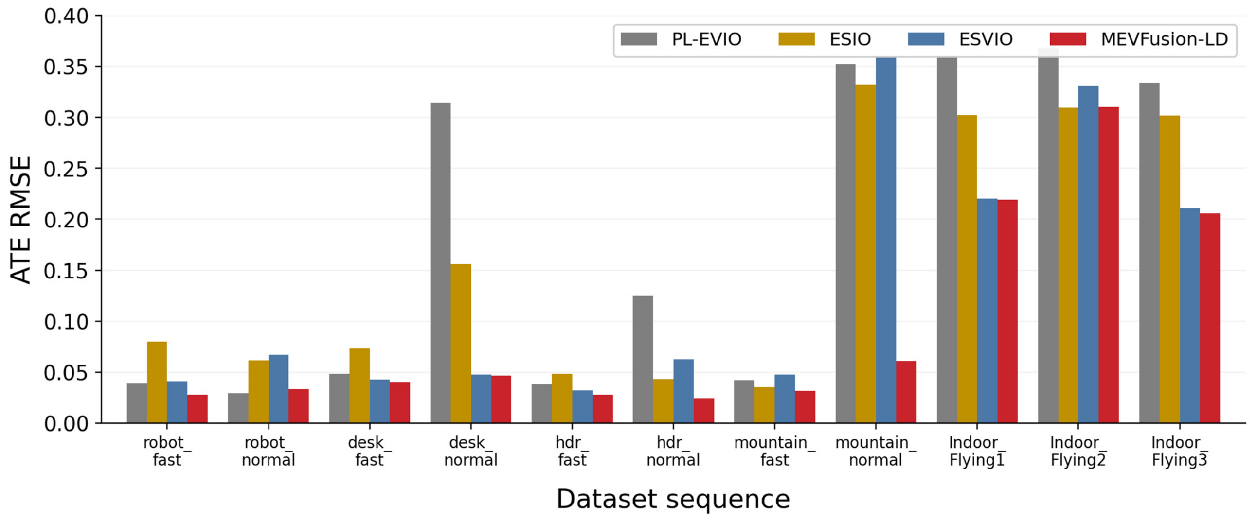
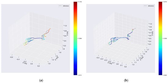
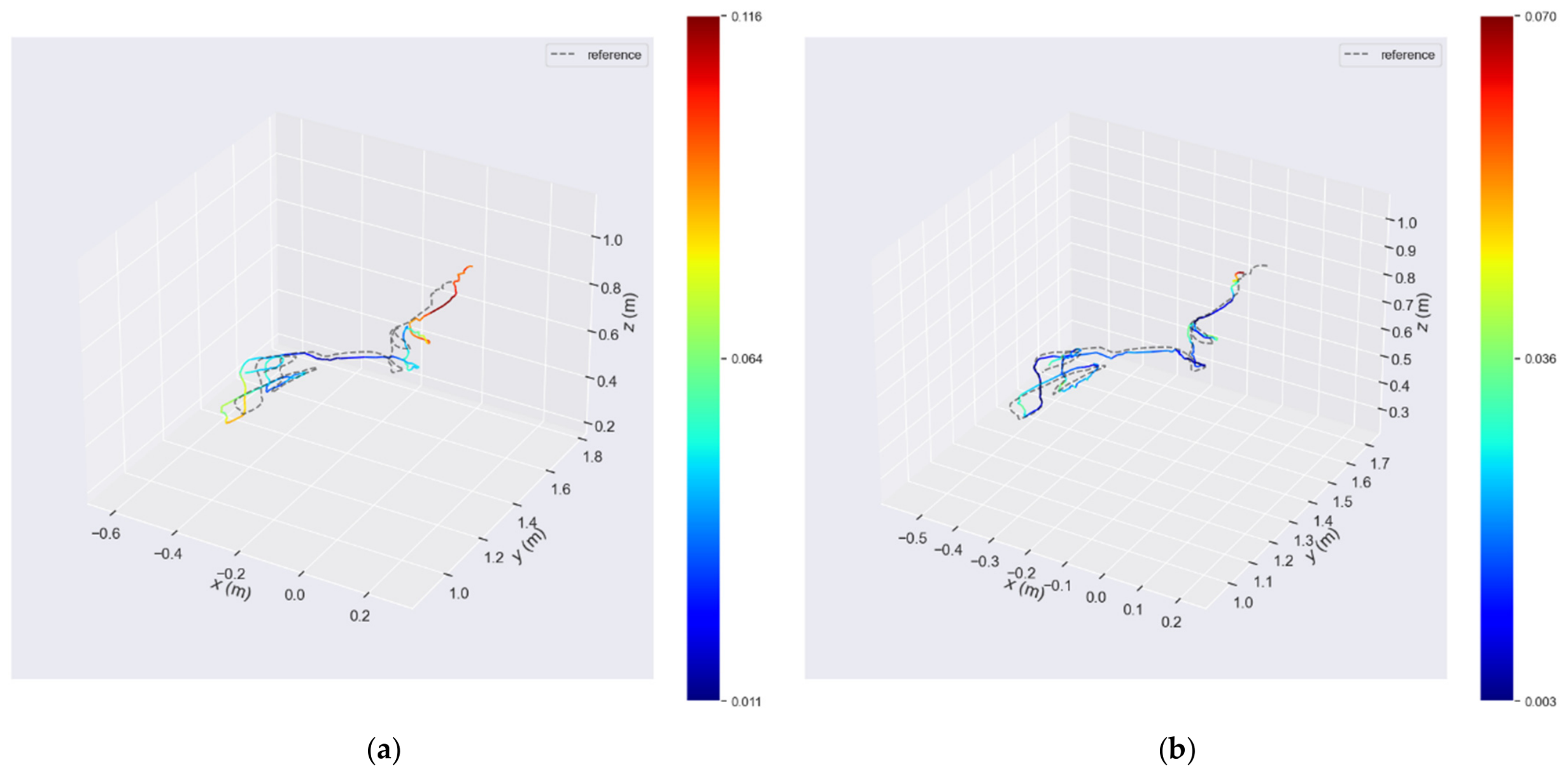
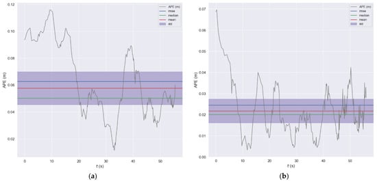
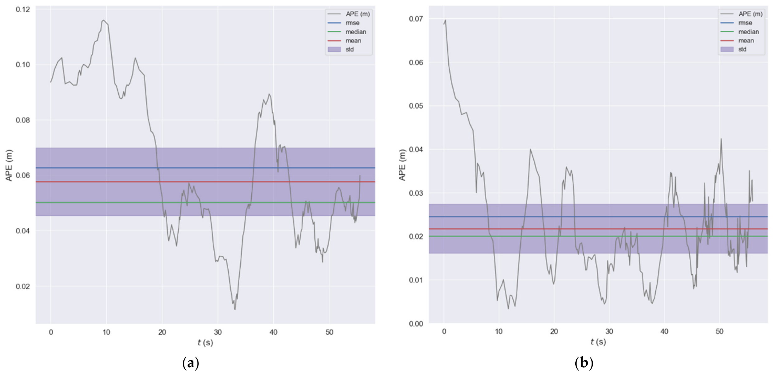
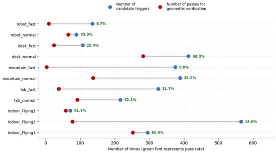
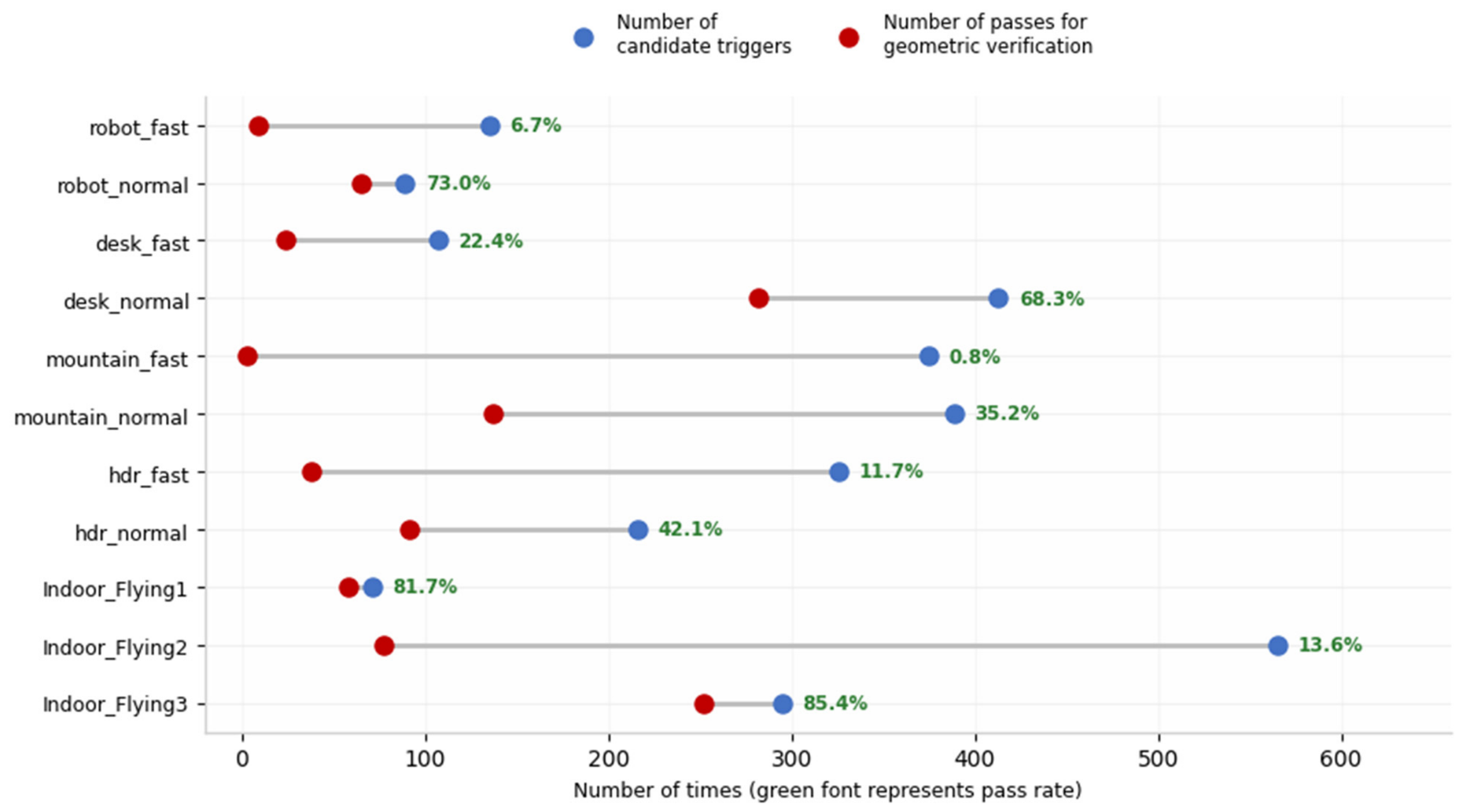
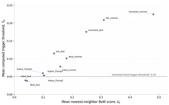
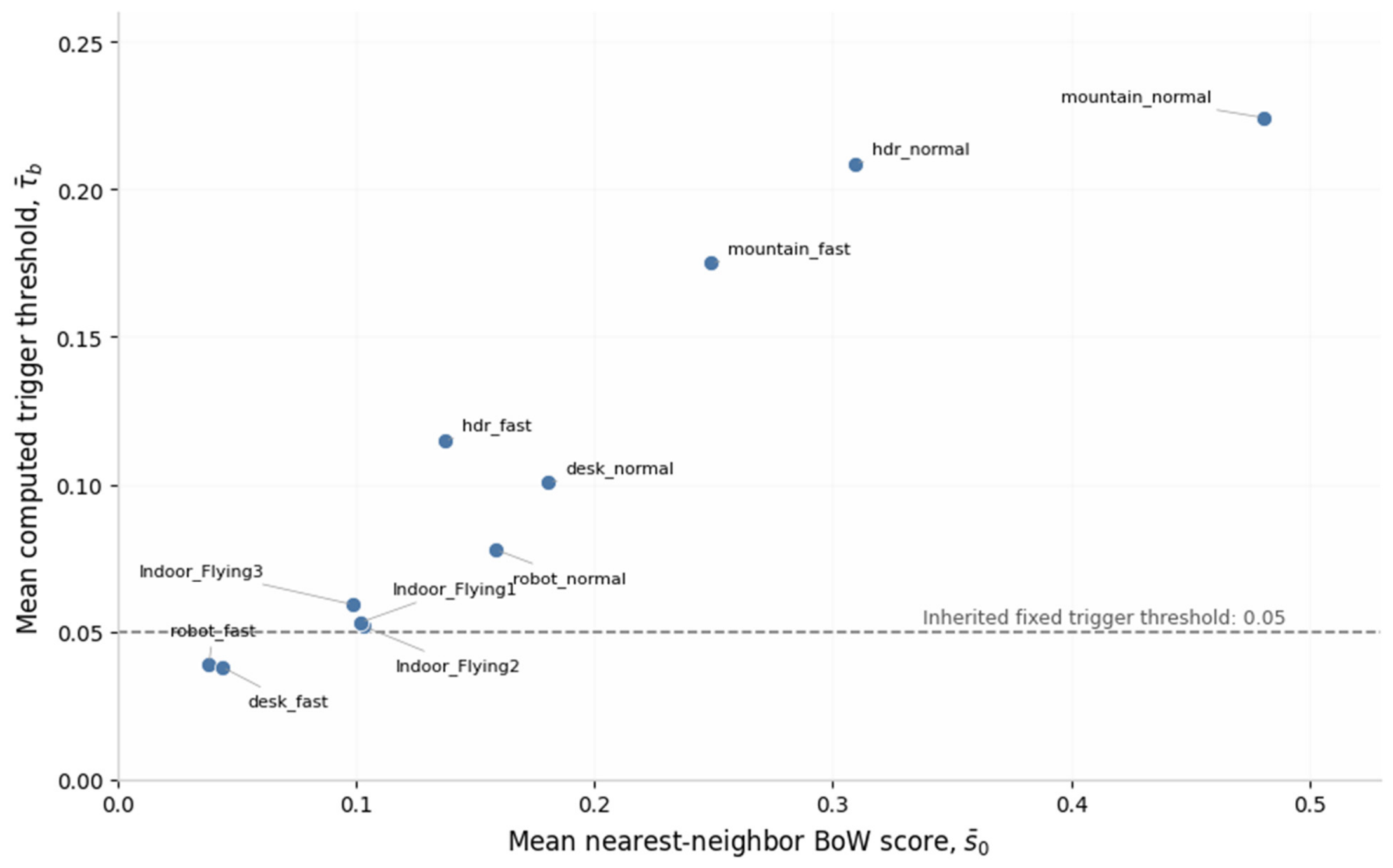
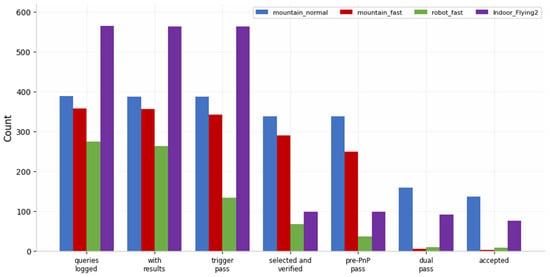
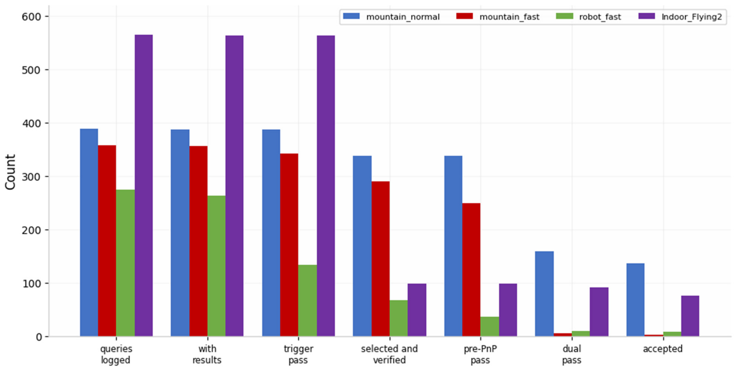
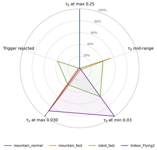
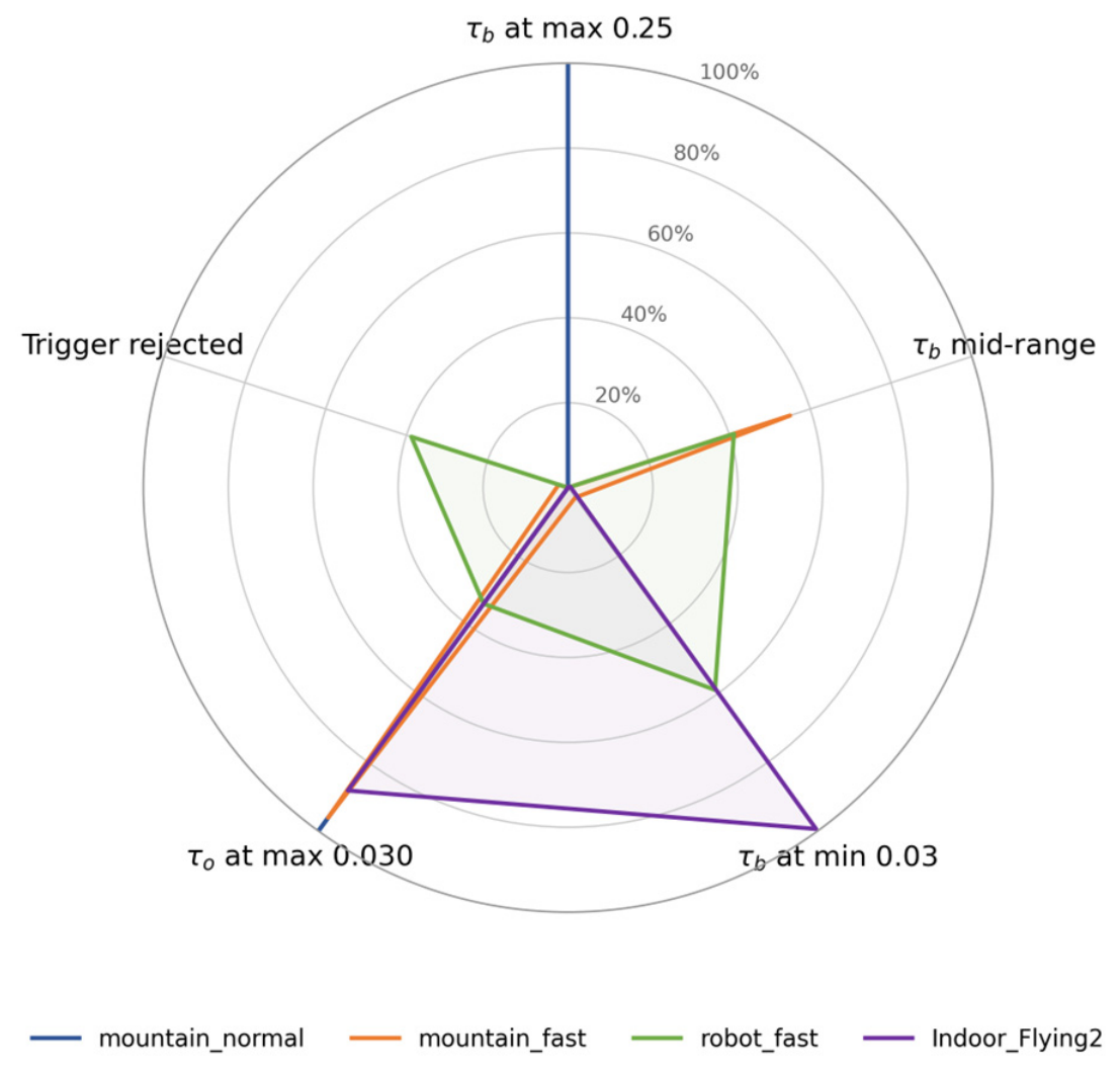
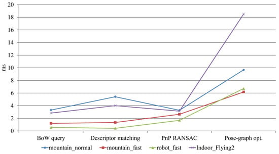
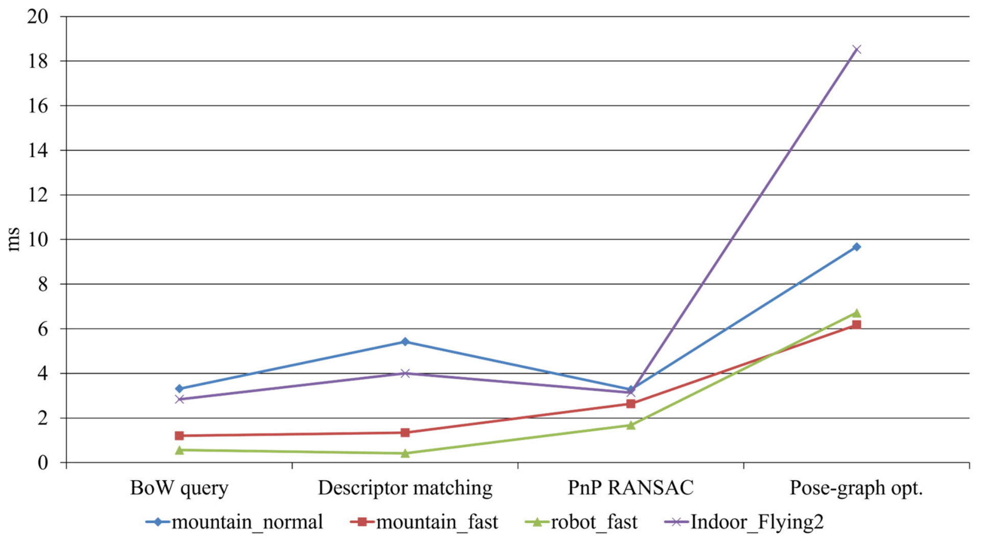

Disclaimer/Publisher’s Note: The statements, opinions and data contained in all publications are solely those of the individual author(s) and contributor(s) and not of MDPI and/or the editor(s). MDPI and/or the editor(s) disclaim responsibility for any injury to people or property resulting from any ideas, methods, instructions or products referred to in the content. |
© 2026 by the authors. Licensee MDPI, Basel, Switzerland. This article is an open access article distributed under the terms and conditions of the Creative Commons Attribution (CC BY) license.