


Highlights
What are the main findings?
- Automated bankfull mapping across Melbourne streams achieved 74% spatial accuracy (F1 score) and 0.64 m mean absolute elevation error.
- Tool reliability mirrors LiDAR visibility limits, performing best in larger streams with low to moderate canopy cover.
What are the implications of the main findings?
- A slope-threshold-based geometry approach works across diverse streams.
- This tool enables catchment-scale channel extent mapping to support geomorphic investigation, flood planning, and waterway management.
Abstract
Accurate and reproducible delineation of stream bankfull geometry remains a persistent challenge in environmental planning. To address this gap, we developed the Cross-Sections and Dimensions Tool, a semi-automated, slope-based method for extracting stream cross-sections and estimating bankfull width, elevation and depth using high-resolution elevation data. The tool applies a configurable slope threshold to identify bank edges, generates perpendicular cross-sections from a stream centreline, and stores all outputs in a structured geodatabase to ensure transparency and reproducibility. Validation against manually delineated bankfull polygons across 191 km of stream length in Greater Melbourne, Australia, demonstrated strong spatial agreement, with an average F1 score (a measure of prediction-observation overlap) of 74% and a mean absolute error of 0.64 m in bankfull elevation. The tool was most reliable in larger streams (Strahler order 5 and above) with low to moderate vegetation canopy cover (<80%). We also investigated the practical visibility limits of small or indistinct channels typically encountered by human mappers and verified that the tool did not produce unrealistic channel delineations. This approach advances geomorphic feature extraction by grounding bankfull delineation in deterministic geometry rather than hydrological recurrence or data-driven modelling. In practice, it enables scalable, transparent, and repeatable analysis of stream morphology for ecological assessment, infrastructure planning, and waterway management.
1. Introduction
Understanding the physical form of river channels is essential for managing hydrological risks, designing resilient infrastructure, and protecting or restoring the health of waterways. Bankfull channel dimensions, in particular, serve as critical indicators of fluvial function, floodplain connectivity, and sediment transport capacity [1]. Accurate bankfull channel delineation provides a foundation for a range of subsequent analyses, including waterway corridor mapping, geomorphic assessments, hydrodynamic modelling and ecological analysis.
While field-based methods for identifying bankfull boundaries offer high accuracy, they are time-consuming and impractical for large-scale applications [2]. Remote sensing has opened new pathways for geomorphic analysis [3]; however, many existing approaches rely on vegetation, sediment or water surface proxies, e.g., [3,4,5], or on hydrological recurrence intervals, e.g., [6], both of which can lack consistency across diverse landscapes [7,8,9].
Hydrological definitions of bankfull flow, such as the 1.5-year recurrence interval, have long been used in practice, e.g., [10], but their variability across catchments [11] and limited relevance in altered flow regimes reduces their usefulness [1]. Morphological definitions, though more robust, often rely on subjective interpretation of sedimentary surfaces or vegetation cues, which are difficult to automate and scale with remote sensing methods, particularly in small streams with overhanging vegetation which obscures in-channel spectral signatures.
Advances in airborne LiDAR technology now allow for near-continuous elevation mapping at sub-meter resolution, offering rich datasets for extracting channel geometry, e.g., [12,13,14]. However, translating raw topographic data into meaningful morphological metrics remains a challenge. LiDAR data issues in small and vegetated streams (e.g., point sparseness, poor classification and unrealistic triangulation; Bowen and Waltermire [15]) pose additional challenges that any method using stream LiDAR data must address. Furthermore, stream-geometry methods must also consider their applicability across different stream types and how they perform in incised, compound, and multi-thread channels. Despite these challenges, objective stream geometry methods based on curvature [16,17,18] or hydraulic depth [12,14] analyses of LiDAR data have achieved good results in various landscapes.
Recent efforts to automate channel delineation using machine learning or neural network-based image segmentation have shown promise in large rivers, but these techniques struggle to detect bankfull boundaries in complex terrain and often lack transparency in their algorithms [19]. Emerging methods using machine learning, deep learning and transfer learning have achieved high predictive accuracy for channel extent and width, e.g., [12,19], yet they remain limited by training data availability and generalisability across different stream types.
To address these limitations, we developed the Cross-Sections and Dimensions Tool—a GIS-based, semi-automated workflow that integrates established slope-based geomorphic principles into a transparent and reproducible framework for large-scale application. Rather than introducing a new definition of bankfull or a novel detection algorithm, the contribution of this tool lies in its ability to operationalise deterministic, geometry-based bankfull delineation consistently across extensive stream networks while explicitly accounting for data limitations and uncertainty.
By generating non-intersecting cross-sections perpendicular to a stream centreline, applying a configurable slope threshold to identify bank edges, and retaining all intermediate datasets, the tool prioritises interpretability, reproducibility, and failure detection. This approach advances the use of deterministic geometry-based methods [20] and robust GIS workflows [21] in fluvial geomorphology. The approach is distinguished from fully automated or data-driven methods that may achieve high predictive performance but offer limited transparency or diagnostic insight when applied outside their training domain. In this paper, we present the conceptual framework, technical implementation, and validation of the tool. We demonstrate its application and assess its performance across 1863 km of streams in varied geomorphic contexts in urban, peri-urban, and rural parts of Greater Melbourne, Australia. Finally, we discuss the implications of the tool for integrating robust, broad-scale estimates of channel form into environmental planning, ecological and geomorphic assessment, and catchment-scale decision-making.
2. Materials and Methods
2.1. Tool Development
To support scalable and reproducible extraction of bankfull channel metrics from LiDAR-derived elevation data, we developed the Cross-Sections and Dimensions Tool—a modular Python (version 3.x)-based workflow built on the ArcPy library and integrated within ESRI’s ArcGIS Pro (version 3.x) environment. The tool automates the generation of station points, 2D and 3D cross-sections, slope-based bankfull extent delineation, and polygonal channel boundary outputs.
2.1.1. Architecture and Workflow
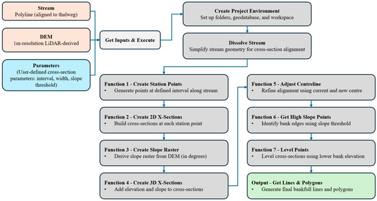
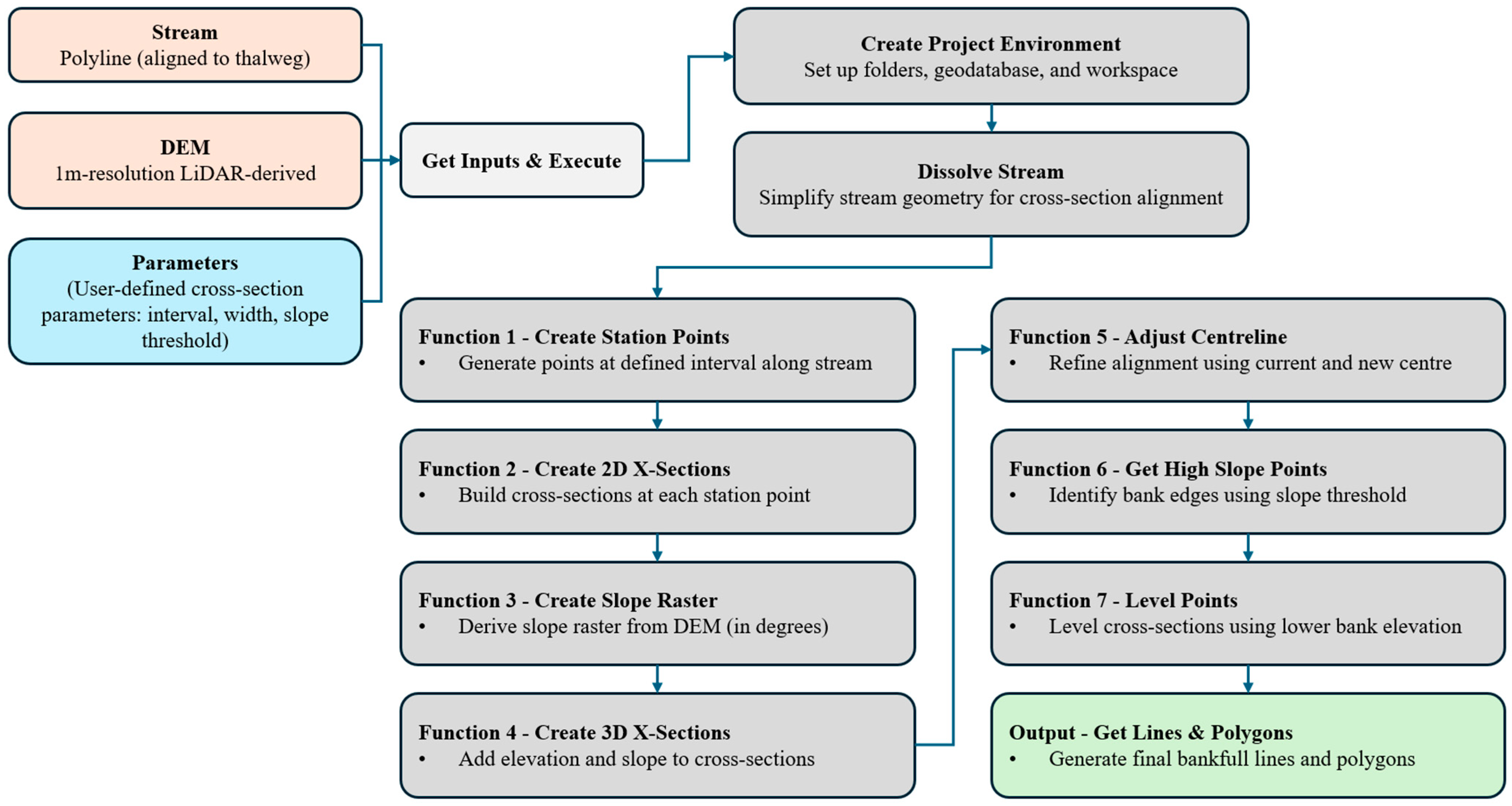
The tool comprises four core functions (Figure 1), each corresponding to a user-defined processing level:
Figure 1.
Workflow of the Cross-Sections and Dimensions Tool.
- Station Point Generation: Using a dissolved stream polyline and a user-specified interval, the tool generates evenly spaced station points along the stream centreline. These points serve as anchor locations for cross-section construction.
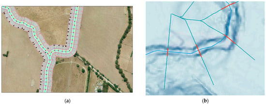
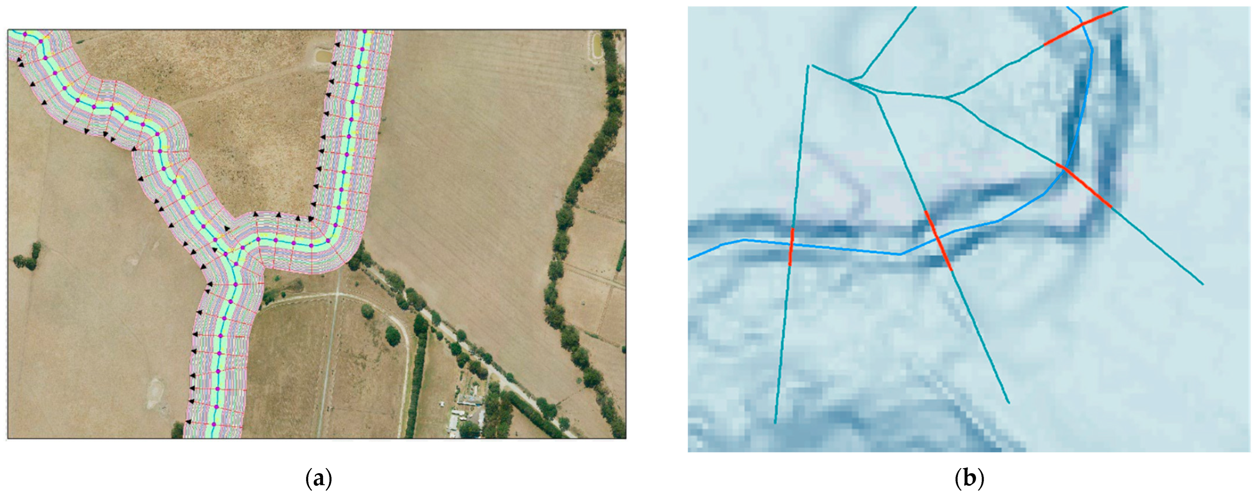
- Two-dimensional (2D) Cross-Section Construction: Pseudo-perpendicular cross-sections are created at each station point, extending to a user-defined half-width. The term “pseudo-perpendicular” is used here because cross-sections are constructed geometrically to be as close as possible to perpendicular to the centreline, while avoiding intersections with adjacent cross-sections in highly sinuous reaches. To construct these geometries, buffer lines are generated at set 1 m intervals outward from the centreline up to the specified half-width. From each station point, perpendicular projections are drawn to intersect these buffer lines, and the resulting points are connected to form the cross-section. This routine produces cross-sections that are as perpendicular as possible to the stream centreline, without crossing other cross-sections (Figure 2). This buffering and cross-section-warping routine ensures that each cross-section crosses the channel only once, even in sinuous reaches, and that the cross-section series provides a reasonable one-dimensional representation of stream morphology. These 2D geometries form the basis for elevation sampling and slope analysis.Figure 2. Visual illustration of process including (a) pseudo-perpendicular cross-section construction approach using concentric buffers of stream centreline, and cross-sections projected perpendicular to buffer boundaries; (b) detail of stream centreline definition (light blue), pseudo-perpendicular cross-sections (teal), and levelled bankfull cross-sections (red) defined using the slope-threshold approach.
- Three-dimensional (3D) Cross-Section Profiling: Elevation values are extracted from the input DEM to convert the 2D cross-sections into 3D profiles. A slope raster (in degrees) is computed from the DEM, and each cross-section point (at 1 m intervals all along the cross-section) is attributed with elevation, slope, and position metrics. The tool also recalculates the centre point (i.e., the lowest elevation point in the cross-section), in cases where the centreline was not perfectly aligned to the minimum elevation of the DEM.
- Bankfull Width Delineation via Slope Threshold: A slope-based filtering process is used to identify high-gradient points along each cross-section, representing potential bank edges. Points exceeding a user-defined slope threshold serve as inputs to this process. First, elevation values on both the left and right sides are compared and trimmed based on the minimum of the maximum elevations on each side. Next, gaps within the point sequence are analysed; if a gap spans more than three consecutive points, the process stops at that location and the data are re-trimmed. The resulting points are then levelled to create consistent bankfull profiles, which are subsequently converted into polylines (Figure 2) and polygons. For polylines, the bankfull elevation, width and depth of each cross-section are calculated and recorded in fields. Care must be taken when interpreting the bankfull depth, as standing water in the channel at the time of LiDAR capture may obscure the actual depth of the channel. The recorded depth reflects the depth from bankfull elevation to the minimum elevation of the DEM along the cross-section.
2.1.2. Technical Implementation
The tool is structured around a central Python script that orchestrates function calls from a custom module (GraceGIS_x_sections_functions). The tool prompts the user to provide several key inputs required for processing. These include the project folder location, the coordinate reference system, and the paths to the input stream layer and the 1 m DEM. Additionally, the user must specify the interval between station points, the cross-section width, and the slope threshold, which is used to identify high-gradient points for bank-edge detection. The slope threshold is an important parameter for the identification of top of bank and should be locally calibrated to manually delineated channel extent data. Setting other parameters relies on an understanding of the likely maximum bankfull width in the dataset and the desired output cross-section density. Key operations include the following:
- Input Handling: get_inputs() prompts the user for stream and DEM paths, interval and width parameters, slope threshold, and projection settings.
- Environment Setup: create_project_environment() establishes a workspace and geodatabase structure.
- Stream Preprocessing: dissolve_stream() simplifies the input stream geometry into contiguous lengths for consistent cross-section alignment. This means the tool is robust to inputs of stream centrelines fragmented by reach.
- Cross-Section Generation: create_station_points() and create_2D_x_sections() produce the base geometries of station points and cross-section points and lines.
- Elevation and Slope Attribution: create_slope_raster() and create_3D_x_sections_pts_z_slope_sort_value() enrich cross-section points with topographic metrics (elevation and slope).
- Centreline Adjustment: create_3D_x_sections_pts_cur_new_centre() refines the centre point of each cross-section.
- Bankfull Extraction: get_pts_high_slopes() and x_sec_level_points() apply slope-based filtering and levelling.
- Output Construction: get_lines_poly() generates final levelled bankfull line and polygon features representing bankfull channel extent.
2.1.3. Transparency and Reproducibility
Unlike many machine learning models, the tool provides full transparency in its logic and outputs. All intermediate datasets are stored in a structured geodatabase, allowing users to inspect, validate, and calibrate results. Temporary files are systematically deleted to maintain workspace hygiene and reduce data storage requirements. Files are labelled with the parameter values used, ensuring traceability when multiple parameter sets are tested. If the parameters are altered and the tool is rerun, existing intermediate outputs are re-used where possible to minimise processing time. For example, if the user changes the slope threshold, the early steps of the routine are not rerun; instead, the existing 3D cross-section points are used for input to the bankfull-extraction step (Function 6 and 7, Figure 1).
2.2. Study Area
The tool was applied and validated across multiple streams in Greater Melbourne, Victoria, Australia, encompassing a range of urban, peri-urban, rural, and forested catchments. It was applied to 1863 km of the stream network. Application was limited to streams of Strahler order 3 and above, corresponding to streams approximately 5 m wide and larger. Streams smaller than 5 m are generally not sufficiently represented in a 1 m resolution DEM to accurately delineate bankfull extent. The spatial extent was also filtered according to the planned end use of the data (investigating stormwater impacts on stream geomorphology): to reaches within 5 km of urban growth areas or established urban landscapes, and within defined stormwater management priority zones [22].
LiDAR DEMs with a resolution of 1 m are available across the region from the 2017–2018 Greater Melbourne LiDAR dataset [23], which has a horizontal accuracy of 0.2 m and a vertical accuracy of 0.1 m (1 σ). Channel alignments are available from the Melbourne Water Stream Network [24]. These alignments required minor editing to be used as channel centrelines in this study (to position them as close as possible to the low points in the LiDAR DEM).
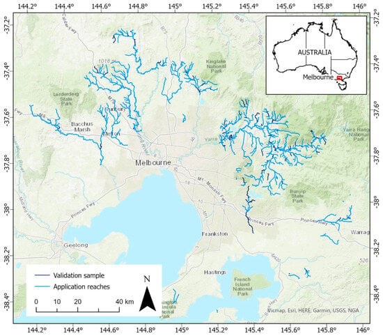
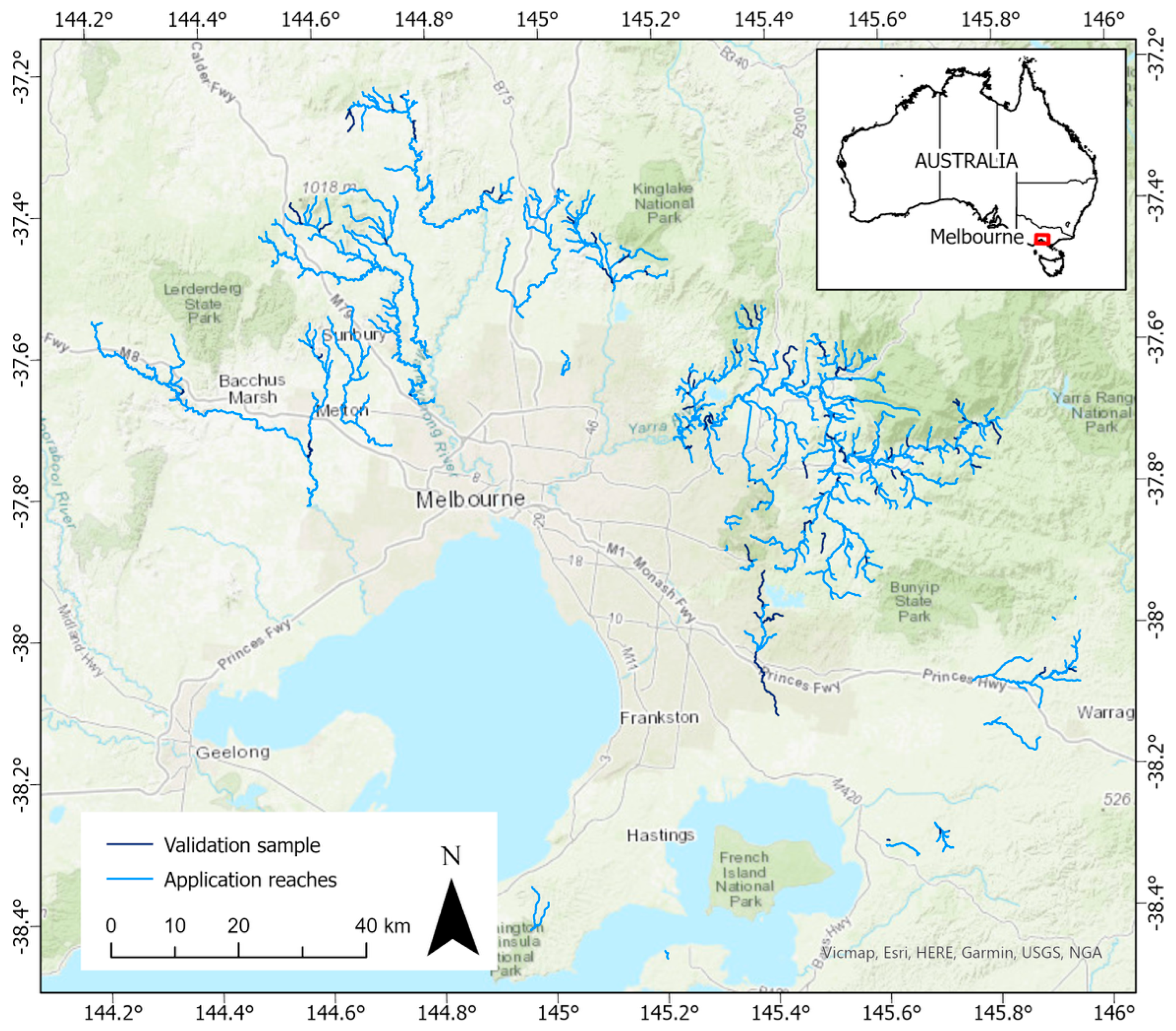
Calibration of the slope threshold parameter was undertaken on 48 km of stream length, selected to represent the range of stream sizes and types across the region. The calibrated slope threshold was then applied to the whole application area. Detailed validation and performance evaluation were undertaken across 191 km of the stream network (10% of the total), randomly sampled from the application area. The sampled streams were similarly distributed to the overall population in terms of stream order and geographic location (Figure 3).
Figure 3.
Study area, showing validation and application stream reaches across the Greater Melbourne region.
2.3. Validation
2.3.1. Validation Data
We manually digitised reference bankfull polygons based on geomorphic interpretation of the morphological top of bank. The top of bank was defined as the break in slope at the upper margin of the stream bank, immediately before transition to the lowest floodplain on each side. Reference bankfull delineation was undertaken through systematic visual inspection of the LiDAR DEM (the same dataset used by the tool), supported by derived slope and curvature rasters and high-resolution aerial imagery. These datasets were used together to identify consistent breaks in slope, changes in surface roughness, and floodplain continuity indicative of bankfull extent.
Once polygons of the reference morphological bankfull extent were delineated (which did not necessarily have the same bankfull elevation on both sides), they were converted to levelled bankfull cross-sections to ensure comparability to the tool outputs. Three-dimensional cross-sections generated by the Cross-sections and Dimensions Tool (prior to bankfull extent delineation, levelling and trimming) were intersected with the manually delineated bankfull extent polygons. The elevation of the lower bank was then calculated for each cross-section, and the reference bankfull extent was trimmed to exclude elevations above the lower bank elevation, producing a levelled reference extent.
It is acknowledged that both the tool outputs and the reference bankfull delineations were derived from interpretation of the same LiDAR DEM. This introduces a degree of same-source bias because errors in the LiDAR data will carry through to both the reference data and the tool outputs. As such, this validation method does not evaluate the ability of LiDAR data to represent a stream channel accurately; rather, it evaluates the ability of the Cross-sections and Dimensions Tool to extract channel boundaries from a given LiDAR dataset in comparison with a human operator. This approach is consistent with established practice in LiDAR-based geomorphic studies [12,16,17], and the independent, expert-led manual interpretation provides a meaningful benchmark against which to evaluate the internal consistency, repeatability, and practical reliability of the automated delineation.
Additionally, to test how representative the tool-derived cross-sections were of observed channel geomorphology on the ground, further validation was undertaken using a field dataset collected in 2024 at 71 sites by geomorphologists unrelated to this study (unpublished data collected by Streamology and provided by Melbourne Water). At each site, an initial estimate of the bankfull width was made, and the spacing between cross-sections was set at the bankfull width. Fifteen cross-sections were measured at each site along a reach length of 15 times the bankfull width. At each cross-section, the bankfull width was measured from the top of one bank to the other, where water just begins to overflow onto the floodplain. For field validation, the Cross-sections and Dimensions Tool was run for each surveyed reach extent, with cross-section spacing the same as the spacing used in the field survey.
2.3.2. Performance Metrics
Bankfull extent validation metrics were based on the overlap between the predicted and reference cross-sectional bankfull extent, using only the cross-sections for which both the tool and the manual delineation were able to produce a bankfull cross-section. Cross-sectional overlap metrics were used in preference to area-based polygon overlap metrics because the tool directly generates bankfull extent by cross-sections. The tool also creates a polygon bankfull extent by connecting together bankfull cross-section ends but, this step does not add any new information. Its accuracy is dependent on the cross-section spacing relative to the channel size and sinuosity. Evaluating overlap metrics on cross-sections rather than polygons reduces sensitivity to local planform complexity and allows performance to be assessed consistently across reaches of varying width, sinuosity, and cross-section density.
For each cross-section, the lengths of the cross-section classified as true positive (TP) (within both the predicted and reference extents), false positive (FP) (within the predicted but not the reference extent), and false negative (FN) (within the reference but not the predicted extent) were computed. The lengths of TP, FP and FN were then aggregated over a reach or a tile to provide overall measures of the accuracy of the extent:
Precision = TP/(TP + FP)
Recall = TP/(TP + FN)
F1 = 2TP/(2TP + FN + FP)
Precision indicates how much of the predicted extent is correct according to the reference, while recall indicates how much of the reference extent is covered by the prediction. The F1 score is the geometric mean of precision and recall, providing a balanced evaluation metric. Precision is also known as the positive predictive value or user’s accuracy, while recall is also known as sensitivity or true positive rate or producer’s accuracy, with different terminology in use in different fields of study. The F1 score is also known as the Dice coefficient (the terminology that was used by Garber, Thompson, Burns, Kunapo, Zhang and Russell [12]). F1 scores over 0.8 are considered excellent for this dataset. Given the fuzzy nature of manual bankfull delineation, we expect some error in the validation data. For example, if we were to compare two expert geomorphologists, we would expect to achieve only around 90% agreement between them (i.e., F1 score of around 0.9) [12,25]. Therefore, F1 scores approaching and exceeding 0.9 for our data represent the upper limit of meaningful accuracy.
Bankfull elevation validation metrics were computed by calculating the difference between the predicted and reference bankfull elevation for each cross-section, then computing mean error (ME) and mean absolute error (MAE). ME (the mean of predicted minus reference elevation) indicates the tendency of the model to underpredict or overpredict systematically, while MAE (mean absolute difference between predicted and reference values) indicates the tendency of the model to deviate regardless of direction.
For validation against field data, validation relied on comparison of mean bankfull width for the surveyed reach (mean of 15 cross-sections per site). Cross-sectional overlap metrics and bankfull elevation metrics could not be used, as the exact locations of the field cross-sections and bankfull elevations were not recorded. We computed the difference between predicted and field mean bankfull widths, then the ME and MAE in bankfull width.
2.3.3. Slope Threshold Calibration
The most important user-defined parameter for the calculation of bankfull width is the slope threshold, which should be locally calibrated to manually delineated data. Slope thresholds of 7, 9, 11 and 13° were tested on 48 km of stream length across four DEM tiles selected from the application area. Calibration reaches were selected to represent a wide range of performance outcomes (following initial testing with a 7° threshold). The slope threshold producing the highest F1 scores and the lowest mean error and mean absolute error across the majority of calibration reaches was selected for application across all study reaches.
2.3.4. Validation, Quality Coding and Limits of Applicability
For 191 km of channel sampled across Greater Melbourne, performance metrics were calculated, and their relationships with landscape properties representing stream size and vegetation cover—two variables expected to influence the accuracy of LiDAR data and derived channel cross-sections—were assessed. Strahler stream order (representing stream size) for each reach was sourced from the Melbourne Water Stream Network [24], and canopy cover within a 5 m buffer of the stream was sourced from unpublished 2018 raster data. Strahler order is used here as a simple and consistently available proxy for relative stream size rather than as a comprehensive descriptor of channel morphology, enabling stratified evaluation of tool performance without introducing additional derived variables. In regions where stream order is unavailable, upstream catchment area or other proxies for stream size could be substituted without altering the workflow. We developed a quality-coding system based on stream order and canopy cover, applicable to the Melbourne region, which may serve as a useful initial guide elsewhere, given widespread availability of these parameters.
Furthermore, we examined the tool failure rate (i.e., instances where the top of bank was not detected), as well as cases where tool failure occurred despite channel extents being visually discernible in LiDAR data or aerial imagery, and conversely, cases where the tool successfully delineated channel extents that were not visually apparent to the annotator. Channel visibility to the human annotator was assessed using the same information available during reference delineation, namely the LiDAR-derived DEM and supporting high-resolution aerial imagery, viewed concurrently.
2.4. Regional Application
The tool was applied to 1863 km of the stream network across Greater Melbourne, enabling semi-automated extraction of bankfull metrics across diverse catchments. Its modular design supports flexible deployment across varied geomorphic settings, including incised channels, vegetated corridors, and engineered waterways. Parameters applied were a cross-section spacing of 25 m, a cross-section half-length of 30 m, and a slope threshold of 11°.
3. Results
3.1. Slope Threshold Calibration Results
A slope threshold of 11° performed best for three of the tested DEM tiles, and was equal-best for one tile (Table 1). For the worst-performing tile (tile 1), the F1 score increased from 0.52 with a threshold of 7° to 0.57 with a threshold of 11°, and the mean error decreased from 1.13 m to 1.00 m. For the best-performing tile (tile 4), the F1 score increased from 0.83 to 0.84, and the mean error decreased from 0.19 to 0.09 m. Therefore, 11° was adopted as the slope threshold for regional application.
Table 1.
Comparison of performance of slope threshold for four selected LiDAR tiles. Green shading indicates the best-performing slope threshold for each tested tile. ME = mean error; MAE = mean absolute error.
3.2. Validation Results
For all validated cross-sections (n = 5351), the overall F1 score was 0.74 (Table 2). There was a tendency to overestimate extents and elevations. On average, the tool missed around 24% of the reference extent of the bankfull width (recall = 0.76), and approximately 28% of the predicted extent was incorrect (precision = 0.72). The mean absolute error in bankfull elevation was 0.64 m, which was around 30% of the mean channel depth (2 m) across the validation sample.
Table 2.
Quality code definition and performance evaluation for each quality class and for all data, showing precision, recall and F1 score of bankfull width extent, and mean error (ME) and mean absolute error (MAE) in bankfull elevation. “Order” refers to Strahler order on the stream network.
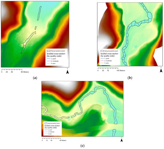
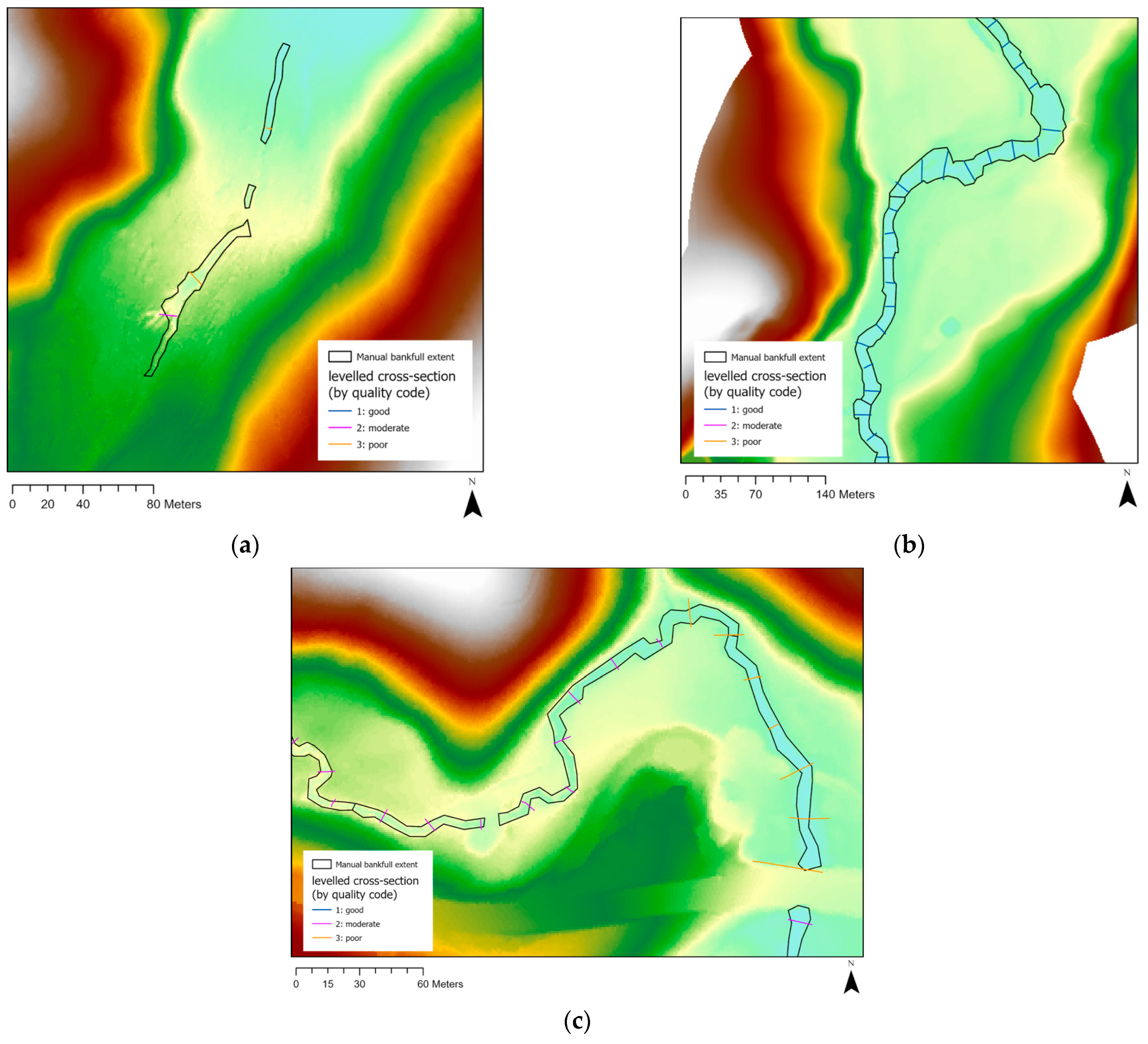
The tool failed on 17% of validation cross-sections, and a partially overlapping set of 17% of cross-sections were not visible to the human eye during manual delineation with a LiDAR DEM and aerial imagery (Table 3). Tool failure is an important feature, as it prevents meaningless outputs when the inputs do not allow reasonable channel delineation. The tool fails if a bank is not detected at all (i.e., when the slope never exceeds the slope threshold along the cross-section) or if the top of bank is not detected (i.e., when the slope, after exceeding the threshold, never drops below it again on either side of the channel centreline). This occurs in cases where the channel is too small to be represented by the resolution of the LiDAR digital elevation models, where the channel is wide and shallow with poorly defined banks, where the channel does not exist (e.g., it has been piped or re-aligned), and where canopy cover prevents LiDAR ground strike points and disrupts channel definition in the LiDAR DEM (see Figure 4a).
Table 3.
Confusion matrix for visibility of channel to manual annotator and tool success/failure.
Figure 4.
Visual examples of data quality: (a) where the channel is not easily discernible in LiDAR data and tool mostly fails to delineate bankfull extent; (b) in good quality-coded reach; and (c) in moderate and poor quality-coded reaches. The manual reference bankfull extent is shown in black and cross-section data quality by coloured lines (dark blue = good, magenta = moderate, orange = poor).
Where the manual annotator judged the channel to be visible, the tool successfully detected a bankfull channel width for 88% of those cross-sections and failed for 12%. Where the annotator judged the channel not visible, the tool had a 45% chance of also failing to detect a bankfull channel width. This indicates that the tool generally performed well in identifying a channel in the same places as the human did, but where the channel was not discernible to the human eye, the tool misidentified a channel in around half of these cases. Overall, we expect roughly 10% of the tool’s bankfull cross-sections to be in areas where the channel is not visually apparent.
Strahler order and local canopy cover both affected tool accuracy (Table 4). Strahler order is used here as a simple and widely available proxy for relative stream size rather than as a comprehensive descriptor of channel morphology. Other proxies for stream size (e.g., upstream catchment area or bankfull discharge where available) could be substituted for Strahler order without altering the workflow. The tool performed best in streams with canopy cover below 80% and Strahler order greater than or equal to 5 (average F1 = 0.8). The results of this analysis were used to develop a quality coding strategy (Table 2) which can be used to assess output quality or to select locations where the tool has the greatest expected accuracy. Examples of cross-sections tagged as good quality are shown in Figure 4b, and examples of moderate and poor quality-coded cross-sections are shown in Figure 4c to illustrate typical levels of agreement with the manual bankfull extent for the three quality classes.
Table 4.
Tool performance (F1 scores) for categories of Strahler order and canopy cover (proportion). Missing values indicate no validation data available in that category.
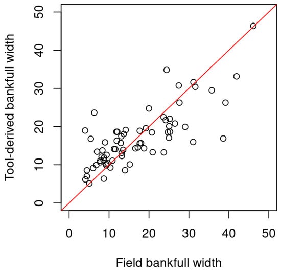
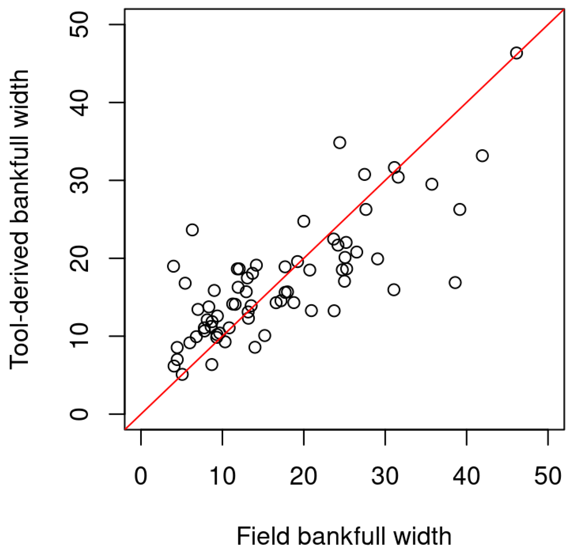
Field validation resulted in ME in bankfull width of 0.06 m, and MAE of 4.7 m. When error was expressed in percentage terms of the field-measured mean bankfull width, the ME was 20%, and the MAE was 40%. Absolute errors were greater for larger streams, while percentage errors were greater for smaller streams. Bankfull widths were particularly prone to overestimation by the tool for streams under 10 m wide, and slightly prone to underestimation for streams over 20 m wide (Figure 5). For comparison, the ME in bankfull width for the overall validation dataset against the reference LiDAR-based bankfull delineation was 0.8 m, and the MAE was 4.9 m, indicating that the tool performed approximately equally well in predicting field-measured and LiDAR-measured bankfull width.
Figure 5.
Field validation result, comparing mean bankfull width derived from the Cross-Sections and Dimensions Tool and field-measured mean bankfull width at 71 sites across the region. 1:1 line is shown in red.
3.3. Application
The tool was successfully applied across 1863 km of the stream network, producing over 74,000 bankfull cross-sections that were then quality-coded (see Table 2). The tool failed to delineate the top of bank for 17% of cross-sections, the same rate as was expected from the validation. Of the cross-sections that were successfully delineated, 39% were classified as good quality, 36% were moderate quality, and only 25% were poor quality.
4. Discussion
4.1. Strengths and Innovations
The Cross-Sections and Dimensions Tool presents a significant advance in semi-automated channel geometry extraction, particularly for small and complex stream networks. Its slope-threshold approach offers a morphologically grounded alternative to hydrological recurrence-based definitions, enabling consistent delineation of bankfull extent across varied terrain and altered hydrology (e.g., regulated or urban streams). The tool’s modular design allows users to calibrate key parameters—such as cross-section spacing, half-width, and slope threshold—tailoring outputs to local geomorphic conditions.
Unlike many machine learning models, the tool is deterministic and provides full transparency in its logic and intermediate outputs. Each processing step is traceable, and all spatial products (e.g., station points, cross-sections, channel boundary polygons) are stored in a structured geodatabase, facilitating validation, refinement, and integration into broader workflows. The tool’s compatibility with ArcGIS Pro ensures accessibility for practitioners and researchers who are already working within established GIS environments.
The tool’s cross-section definition method prevents intersecting cross-sections even in highly sinuous reaches, producing alignments that are consistent with river space. The routine prevents issues produced by cross-sections which intersect each other or cross the stream multiple times, which can challenge hydraulic modelling and other analyses, e.g., [26,27]. As well as being highly suitable for bankfull geometry extraction, the cross-sections produced can be used for other applications such as constructing hydraulic modelling meshes.
Validation results from across Greater Melbourne demonstrate strong agreement with expert-delineated bankfull polygons digitised from LiDAR DEMs and aerial imagery, with an average F1 score of 0.74 and mean absolute error in bankfull elevation of 0.64 m. The tool performed particularly well in downstream reaches (Strahler order 5 and above) with low to moderate vegetation canopy (<80%). Its ability to level cross-sections based on the lower bank elevation enhances consistency in bankfull width estimation. The observed mean absolute error in bankfull elevation (0.64 m) is comparable to uncertainties associated with manual interpretation of LiDAR-derived bankfull indicators and represents approximately 30% of the mean channel depth across the validation dataset. For planning-scale applications, such as regional geomorphic assessment, corridor mapping, and prioritisation, this level of vertical uncertainty is considered appropriate for relative comparisons between reaches and as input to management decisions, particularly given that bankfull elevation is typically interpreted as a morphological zone rather than a discrete elevation surface.
A range of alternative approaches for delineating channel extent and bankfull geometry have been proposed, including curvature-based [16,18] or hydraulic-depth-based [12,14] geometric methods, machine learning or deep learning classifiers [12,28,29], and multispectral or radar-based remote sensing methods [28,29,30]. Curvature and elevation-derivative approaches can be effective in stream types similar to those assessed by our slope-threshold method, but often require smoothing or scale selection that is difficult to generalise across heterogeneous networks. Machine learning and image-based segmentation methods have demonstrated strong performance in large rivers, yet may lack diagnostic transparency and transferability to new regions or altered channels. Multispectral [3,31,32] and water-surface-based methods, e.g., [33,34], provide valuable complementary information but are less suited to identifying top-of-bank in vegetated or intermittently dry channels. Furthermore, the large spatial resolution of many satellite products (on the order of 100–250 m for radar products and 10 m for many widely used spectral products) limits their applicability to small streams, although recent advances are opening up the use of high-resolution spectral products from small satellites [31,32].
A previous study delineating bankfull channel extents in a subset of our study area (Cardinia Creek) provides an opportunity for direct comparison; Garber, Thompson, Burns, Kunapo, Zhang and Russell [12] achieved F1 scores of 0.83 using a cross-sectional hydraulic-depth-based method and 0.82 using a Convolutional Neural Network (CNN) with transfer learning. We calculated an F1 score of 0.81 for the same subset using the Cross-sections and Dimensions Tool. This result builds confidence that the tool performs comparably to alternative published methods.
The Cross-Sections and Dimensions Tool occupies a complementary niche: it performs similarly to data-driven models and other geometric techniques in predictive accuracy, provides a deterministic, interpretable workflow that can be deployed consistently at catchment scale, explicitly reports failure where data are insufficient, and allows users to calibrate parameters in relation to local geomorphic context.
4.2. Limitations and Applicability
Despite its strengths, the tool has limitations that should be acknowledged. Performance declines in very small channels where slope breaks are subtle or obscured by vegetation. In such cases, the limitation arises from the LiDAR dataset itself, rather than the tool’s calculation method. Therefore, this limitation can only be addressed by field inspection or more detailed data collection (e.g., drone-based LiDAR). The tool also assumes that the stream centreline is accurately aligned with the thalweg; misalignment can affect cross-section alignment and bankfull width calculation (although channel extents are robust to small errors in thalweg position, with a tolerance of 5 m).
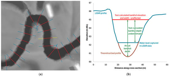
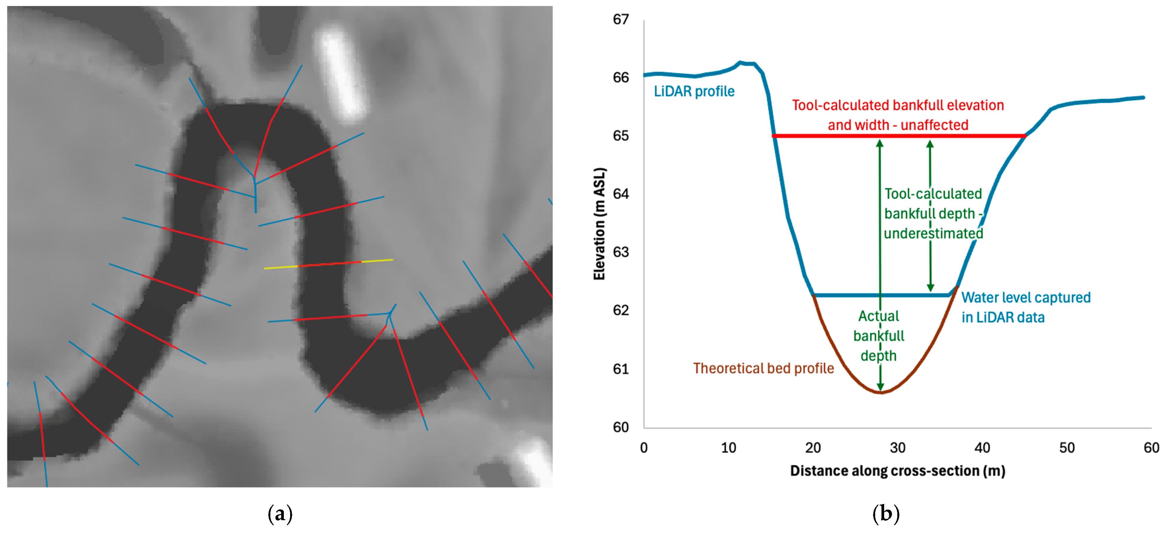
Most DEMs are based on LiDAR data that do not penetrate water. Therefore, in many streams, standing water at the time of LiDAR data capture produces DEMs with flat or triangulated areas across open water areas. These DEM artifacts propagate into the cross-sections delineated by the tool, and the calculation of bankfull depth is therefore likely to be an underestimate of the true bankfull depth except in streams that were dry upon LiDAR capture (Figure 6). This issue does not affect the bankfull elevation or width calculations of the tool.
Figure 6.
(a) Example of LiDAR DEM with standing water obscuring the channel bed; cross-sections are shown in blue, and levelled bankfull cross-sections in red; (b) effect of standing water on LiDAR profile and tool-calculated bankfull depth. The tool-calculated bankfull elevation and width are unaffected by standing water. The plotted profile is highlighted in yellow on panel (a).
The slope-threshold method relies on user-defined values, which may vary between regions and stream types. While this flexibility is a strength, it also introduces subjectivity and requires careful calibration and understanding of local stream geomorphology. The tool does not incorporate hydraulic modelling or sediment transport dynamics, and therefore cannot infer flow regimes or channel capacity, although the produced cross-sections can be used for hydraulic modelling in other software.
Although the slope threshold is locally calibrated, results from the calibration experiment indicate that tool performance varies gradually rather than abruptly across a plausible threshold range (7–13°). This suggests that while absolute accuracy is optimised through local calibration, the method is not overly sensitive to modest threshold mis-specification. In practice, lower thresholds tend to increase recall at the expense of precision (over-prediction of bankfull extent), whereas higher thresholds increase precision while under-detecting subtle banks, particularly in small or vegetated channels. This trade-off is explicit and inspectable within the tool outputs, allowing users to assess uncertainty and refine parameters where required.
4.3. Applications and Future Directions
The tool has immediate applications in waterway and catchment planning, ecological assessment, and infrastructure design. Its outputs can inform riparian buffer zoning, floodplain mapping, and stream condition benchmarking. By enabling consistent extraction of bankfull metrics across large areas, the tool supports regional-scale analysis of channel form and its relationship to land use, vegetation cover, and urbanisation.
Future enhancements could include integration with machine learning classifiers to refine bank detection, e.g., [12], and development of a graphical user interface for non-technical users. Applying the tool to time-series LiDAR data could enable monitoring of channel evolution and incision-recovery trajectories, while further analysis of LiDAR data along the cross-sections could reveal valuable information about streambank conditions (slope, vegetation) and instream geomorphic features.
The tool contributes to a growing body of work that leverages remote sensing and spatial analysis for geomorphic feature extraction [2,9,12]. Its transparent logic, reproducibility, and adaptability position it as a valuable resource for researchers and practitioners seeking scalable solutions to river morphology analysis.
5. Conclusions
This study presents a novel, transparent, and adaptable tool for extracting stream cross-sections and estimating bankfull dimensions using high-resolution elevation data. By leveraging slope-based thresholds and modular parameters, the Cross-Sections and Dimensions Tool enables consistent delineation of channel geometry across diverse landscapes, particularly in small and morphologically complex catchments.
Validation against expert-delineated bankfull extents confirms the tool’s reliability, with strong spatial agreement and minimal error. Its integration within standard GIS environments and structured geodatabase outputs enhances usability, reproducibility, and scalability for both research and applied contexts. While limitations exist in densely vegetated or incised channels, and projection constraints currently restrict geographic scope, the tool offers a robust foundation for future enhancements. Its potential applications span ecological assessment, infrastructure planning, and catchment-scale monitoring, contributing to more informed and data-driven environmental decision-making. By bridging the gap between manual delineation and complete automation, this tool supports a new generation of geomorphic analysis—transparent, efficient, and grounded in spatial logic.
Author Contributions
Conceptualization, J.K. and K.R.; methodology, J.K. and K.R.; software, J.K.; validation, K.R.; writing—original draft preparation, J.K. and K.R.; writing—review and editing, J.K. and K.R. All authors have read and agreed to the published version of the manuscript.
Funding
This work was funded by Melbourne Water under the Melbourne Waterway Research-Practice Partnership (mwrpp.org). The APC was waived by MDPI.
Data Availability Statement
The Cross-Sections and Dimensions Tool Version 2.0 [35] is available under MIT licence (https://doi.org/10.5281/zenodo.18950771 accessed on 1 April 2026). The tool output and validation data and R code used to validate the tool performance [36] are openly available (https://doi.org/10.5281/zenodo.18951275 accessed on 1 April 2026).
Acknowledgments
We are grateful for comments on a draft manuscript provided by Rhys Coleman. Melbourne Water provided LiDAR data and field-measured bankfull width data collected by Streamology.
Conflicts of Interest
The authors declare no conflicts of interest. The funders had no role in the design of the study; in the collection, analyses, or interpretation of data; in the writing of the manuscript; or in the decision to publish the results, but did provide comments on a draft manuscript.
Abbreviations
The following abbreviations are used in this manuscript:
| GIS | Geographic information systems |
| LiDAR | Light detection and ranging |
| DEM | Digital elevation model |
| TP | True positive |
| FP | False positive |
| FN | False negative |
| ME | Mean error |
| MAE | Mean absolute error |
| 2D | Two-dimensional |
| 3D | Three-dimensional |
References
- Bent, G.C.; Waite, A.M. Equations for Estimating Bankfull Channel Geometry and Discharge for Streams in Massachusetts; No. 2013-5155; U.S. Geological Survey: Reston, VA, USA, 2013; p. 62.
- Delchiaro, M.; Ruscitto, V.; Schwanghart, W.; Brignone, E.; Piacentini, D.; Troiani, F. BankfullMapper: A semi-automated MATLAB tool on high-resolution Digital Terrain Models for spatio-temporal monitoring of bankfull geometry and discharge. Comput. Geosci. 2025, 205, 106001. [Google Scholar] [CrossRef] [Scilit]
- Carbonneau, P.E.; Belletti, B.; Micotti, M.; Lastoria, B.; Casaioli, M.; Mariani, S.; Marchetti, G.; Bizzi, S. UAV-based training for fully fuzzy classification of Sentinel-2 fluvial scenes. Earth Surf. Process. Landf. 2020, 45, 3120–3140. [Google Scholar] [CrossRef] [Scilit]
- Li, D.; Xue, Y.; Qin, C.; Wu, B.; Chen, B.; Wang, G. A bankfull geometry dataset for major exorheic rivers on the Qinghai-Tibet Plateau. Sci. Data 2022, 9, 498. [Google Scholar] [CrossRef] [Scilit] [PubMed]
- Xue, Y.; Qin, C.; Wu, B.; Li, D.; Fu, X. Automatic extraction of mountain river surface and width based on multisource high-resolution satellite images. Remote Sens. 2022, 14, 2370. [Google Scholar] [CrossRef] [Scilit]
- Edwards, P.J.; Watson, E.A.; Wood, F. Toward a better understanding of recurrence intervals, bankfull, and their importance. J. Contemp. Water Res. Educ. 2019, 166, 35–45. [Google Scholar] [CrossRef] [Scilit]
- Petit, F.; Pauquet, A. Bankfull discharge recurrence interval in gravel-bed rivers. Earth Surf. Process. Landf. J. Br. Geomorphol. Group 1997, 22, 685–693. [Google Scholar] [CrossRef]
- Fentie, B. Estimating bankfull channel geometry using high-resolution LiDAR DEMs. In Proceedings of the MODSIM 2019 International Congress on Modelling and Simulation, Canberra, Australia, 1–6 December 2019. [Google Scholar]
- Amanambu, A.C.; Mossa, J.; Chen, Y.-H. Redefining Bankfull Stage Using Machine Learning Prediction in a Large Lowland River. Earth Surf. Process. Landf. 2025, 50, e70211. [Google Scholar] [CrossRef] [Scilit]
- Simon, A.; Dickerson, W.; Heins, A. Suspended-sediment transport rates at the 1.5-year recurrence interval for ecoregions of the United States: Transport conditions at the bankfull and effective discharge? Geomorphology 2004, 58, 243–262. [Google Scholar] [CrossRef] [Scilit]
- Williams, G.P. Bank-full discharge of rivers. Water Resour. Res. 1978, 14, 1141–1154. [Google Scholar] [CrossRef] [Scilit]
- Garber, J.; Thompson, K.; Burns, M.J.; Kunapo, J.; Zhang, G.Z.; Russell, K. Artificial Intelligence and Objective-Function Methods Can Identify Bankfull River Channel Extents. Water Resour. Res. 2024, 60, e2023WR035269. [Google Scholar] [CrossRef] [Scilit]
- Johansen, K.; Grove, J.; Denham, R.; Phinn, S. Assessing stream bank condition using airborne LiDAR and high spatial resolution image data in temperate semirural areas in Victoria, Australia. J. Appl. Remote Sens. 2013, 7, 073492. [Google Scholar] [CrossRef] [Scilit]
- De Rosa, P.; Fredduzzi, A.; Cencetti, C. A GIS-based tool for automatic bankfull detection from airborne high resolution DEM. ISPRS Int. J. Geo-Inf. 2019, 8, 480. [Google Scholar] [CrossRef] [Scilit]
- Bowen, Z.H.; Waltermire, R.G. Evaluation of light detection and ranging (lidar) for measuring river corridor topography. JAWRA J. Am. Water Resour. Assoc. 2002, 38, 33–41. [Google Scholar] [CrossRef] [Scilit]
- Passalacqua, P.; Belmont, P.; Foufoula-Georgiou, E. Automatic geomorphic feature extraction from lidar in flat and engineered landscapes. Water Resour. Res. 2012, 48, W03528. [Google Scholar] [CrossRef] [Scilit]
- Arghavanian, A.; Leloğlu, U.M. Extraction and classification of channels from LiDAR in plains by channel tracking. Environ. Model. Softw. 2024, 171, 105838. [Google Scholar] [CrossRef] [Scilit]
- Sofia, G.; Tarolli, P.; Cazorzi, F.; Dalla Fontana, G. Downstream hydraulic geometry relationships: Gathering reference reach-scale width values from LiDAR. Geomorphology 2015, 250, 236–248. [Google Scholar] [CrossRef] [Scilit]
- Zarrabi, R.; McDermott, R.; Erfani, S.M.H.; Cohen, S. Bankfull and Mean-Flow Channel Geometry Estimation Through Machine Learning Algorithms Across the CONtiguous United States (CONUS). Water Resour. Res. 2025, 61, e2024WR037997. [Google Scholar] [CrossRef] [Scilit]
- Dong, P.; Zhong, R.; Xia, J.; Tan, S. A semi-automated method for extracting channels and channel profiles from lidar-derived digital elevation models. Geosphere 2020, 16, 806–816. [Google Scholar] [CrossRef] [Scilit]
- De Rosa, P.; Fredduzzi, A.; Cencetti, C. Geographic information system tools for river evolution analysis. Water 2024, 16, 2512. [Google Scholar] [CrossRef] [Scilit]
- Melbourne Water. HWS2018 Stormwater Priority Areas [Dataset]. 2019. Available online: https://discover.data.vic.gov.au/dataset/hws2018-stormwater-priority-areas (accessed on 1 April 2026).
- Melbourne Water and Department of Transport and Planning. Greater Melbourne LiDAR 2017-18 [Dataset]. 2019. Available online: https://www.land.vic.gov.au/maps-and-spatial/imagery/elevation-data/major-lidar-projects/greater-melbourne-lidar-2017-18 (accessed on 1 April 2026).
- Walsh, C.J. The Melbourne Water Stream Network: User’s Manual. Version 1.3; Melbourne Waterway Research-Practice Partnership Report 19.4d; Waterway Ecosystem Research Group, School of Agriculture, Food, and Ecosystem Sciences, The University of Melbourne: Melbourne, Australia, 2023. [Google Scholar]
- Gob, F.; Thommeret, N.; Bilodeau, C.; Tamisier, V.; Riviere, R.; Kreutzenberger, K. Assessing the morphological alteration of river reaches from 15 years of measurements: French hydromorphological database and indicators (Carhyce). Geomorphology 2025, 479, 109737. [Google Scholar] [CrossRef] [Scilit]
- Bales, J.; Wagner, C. Sources of uncertainty in flood inundation maps. J. Flood Risk Manag. 2009, 2, 139–147. [Google Scholar] [CrossRef] [Scilit]
- Merwade, V.; Cook, A.; Coonrod, J. GIS techniques for creating river terrain models for hydrodynamic modeling and flood inundation mapping. Environ. Model. Softw. 2008, 23, 1300–1311. [Google Scholar] [CrossRef] [Scilit]
- Carbonneau, P.E.; Dugdale, S.J.; Breckon, T.P.; Dietrich, J.T.; Fonstad, M.A.; Miyamoto, H.; Woodget, A.S. Adopting deep learning methods for airborne RGB fluvial scene classification. Remote Sens. Environ. 2020, 251, 112107. [Google Scholar] [CrossRef] [Scilit]
- Buscombe, D.; Ritchie, A.C. Landscape classification with deep neural networks. Geosciences 2018, 8, 244. [Google Scholar] [CrossRef] [Scilit]
- Demarchi, L.; Bizzi, S.; Piégay, H. Hierarchical object-based mapping of riverscape units and in-stream mesohabitats using LiDAR and VHR imagery. Remote Sens. 2016, 8, 97. [Google Scholar] [CrossRef] [Scilit]
- Moortgat, J.; Li, Z.; Durand, M.; Howat, I.; Yadav, B.; Dai, C. Deep learning models for river classification at sub-meter resolutions from multispectral and panchromatic commercial satellite imagery. Remote Sens. Environ. 2022, 282, 113279. [Google Scholar] [CrossRef] [Scilit]
- Valman, S.J.; Boyd, D.S.; Carbonneau, P.E.; Johnson, M.F.; Dugdale, S.J. An AI approach to operationalise global daily PlanetScope satellite imagery for river water masking. Remote Sens. Environ. 2024, 301, 113932. [Google Scholar] [CrossRef] [Scilit]
- Xu, H.; Wu, J.; Yao, J.; Xu, N.; Mo, F.; Li, T.; Lu, Q.; Xia, H.; Zhang, J.; Wang, Y. SDNet: A multi-scale SWOT framework for denoising and quality-control optimization in inland water body extraction. GIScience Remote Sens. 2026, 63, 2636315. [Google Scholar] [CrossRef] [Scilit]
- Tourian, M.J.; Elmi, O.; Mohammadnejad, A.; Sneeuw, N. Estimating river depth from SWOT-type observables obtained by satellite altimetry and imagery. Water 2017, 9, 753. [Google Scholar] [CrossRef] [Scilit]
- Kunapo, J.; Russell, K. Cross-Sections and Dimensions Tool [Software] (v2.0), Version 2.0; Zenodo: Geneva, Switzerland, 2026. [CrossRef]
- Kunapo, J.; Russell, K. Cross-Sections and Dimensions: A LiDAR-Based GIS Tool for Bankfull Channel Mapping [Dataset]. 2026. Available online: https://doi.org/10.5281/zenodo.18951275 (accessed on 1 April 2026).

Disclaimer/Publisher’s Note: The statements, opinions and data contained in all publications are solely those of the individual author(s) and contributor(s) and not of MDPI and/or the editor(s). MDPI and/or the editor(s) disclaim responsibility for any injury to people or property resulting from any ideas, methods, instructions or products referred to in the content. |
© 2026 by the authors. Licensee MDPI, Basel, Switzerland. This article is an open access article distributed under the terms and conditions of the Creative Commons Attribution (CC BY) license.