Global Inversion of Terrestrial Net Ecosystem Exchange: Integrating Explicit Multi-Source Predictors and High-Dimensional Remote-Sensing Embeddings

Highlights

What are the main findings?

• Incorporating AlphaEarth high-dimensional embeddings reduces prediction errors and suppresses spatial noise. Improvements are most evident in regions with complex land surface heterogeneity, compared with conventional explicit predictors.
• Over 2000–2024, global terrestrial NEE exhibits stable large-scale spatial patterns, with stronger net carbon uptake in low latitudes. Interannual variability is dominated by changes in magnitude rather than spatial reorganization.

What are the implications of the main findings?

• High-dimensional embeddings improve global carbon flux estimation without adding new process assumptions. They integrate information from multiple data sources and reduce noise, leading to more stable and consistent results on the global scale.
• Because spatial patterns remain stable and variability is mainly reflected in magnitude, changes in global NEE are driven by how strong carbon exchange is, rather than where it occurs. This means long-term carbon assessments should focus on capturing year-to-year sink intensity changes instead of redefining spatial patterns.

Abstract

Terrestrial ecosystems play a critical role in regulating atmospheric CO₂ through land–atmosphere carbon exchange. While Net Ecosystem Exchange (NEE) serves as a key integrative metric for carbon dynamics, its robust global estimation remains challenging due to profound environmental heterogeneity and nonlinear ecosystem responses. In this study, we propose a dual-track experimental framework to invert annual global terrestrial NEE at a 0.1° spatial resolution for 2000–2024. Initially, a long-term historical baseline inversion (2000–2024) was developed using explicit multi-source environmental predictors. Subsequently, to overcome the representational limitations of conventional spectral indices over complex terrains, we integrated high-dimensional remote-sensing embeddings from the AlphaEarth framework for the 2017–2024 overlapping period. This approach was designed to explicitly quantify the added value of these advanced features. Our results demonstrate that embedding features substantially enhance inversion performance, reducing prediction errors and improving spatial coherence. Adopting the standard meteorological sign convention, global terrestrial NEE remained consistently negative. Based on the 2000–2024 baseline inversion, our predicted global NEE fluctuated between −3.50 and −4.38 Pg C yr⁻¹. To validate these long-term estimates, we systematically cross-validated our results against an independent, recently published multi-network fusion dataset, which reported a comparable range of −3.11 to −3.75 Pg C yr⁻¹. This comparison demonstrates consistent interannual dynamics and corroborates the magnitude of the global terrestrial carbon sink. Spatial patterns exhibit a stable latitudinal structure, with stronger net carbon uptake in low latitudes. Interannual variability is expressed mainly as magnitude fluctuations rather than systematic spatial reorganization. Overall, this study highlights that high-dimensional Earth observation embeddings provide significant, measurable information gains for global NEE inversion without introducing new process-based assumptions, thereby offering a robust and internally consistent basis for evaluating long-term carbon dynamics.

1. Introduction

Terrestrial ecosystems play a pivotal role in the global carbon cycle amidst ongoing climate change. The exchange of carbon between the land surface and the atmosphere directly regulates atmospheric carbon dioxide (CO₂) concentrations, thereby influencing long-term climate dynamics. Net Ecosystem Exchange (NEE), defined as the net balance between ecosystem carbon uptake via photosynthesis and carbon release through autotrophic and heterotrophic respiration, serves as a fundamental metric for diagnosing the source–sink status of terrestrial ecosystems and its temporal variability [1,2]. Consequently, achieving a robust, spatially continuous quantification of global terrestrial NEE and its interannual variability is critical. Such spatiotemporal mapping is essential for elucidating climate–carbon feedbacks, constraining global carbon budget uncertainties, and supporting advanced climate scenario simulations [3].

Conceptually and observationally, NEE is a highly complex metric, representing the integrated response of vegetation physiology, ecosystem respiration, and localized climatic drivers. Its spatiotemporal dynamics are deeply governed by meteorological conditions, ecosystem types, and canopy structural characteristics. Because NEE exhibits pronounced temporal nonlinearity and asymmetry, alongside strong spatial heterogeneity, accurately characterizing its dynamics from regional to global scales remains a persistent challenge. Consequently, despite continued advances in global carbon budget assessments, substantial discrepancies remain among existing NEE products and estimation approaches, underscoring persistent uncertainties in our understanding of global terrestrial carbon exchange [4,5].

Methodologically, the quantification of global NEE is fundamentally driven by a triad of approaches: eddy covariance (EC) observations, process-based ecosystem models, and data-driven remote-sensing upscaling. While EC systems represent the gold standard for directly measuring continuous, high-frequency land–atmosphere CO₂ fluxes, their limited spatial footprints restrict them to localized, site-level assessments [1,6]. To achieve spatially explicit global coverage, process-based models are widely employed to simulate physiological mechanisms. Yet, their performance is inherently constrained by sensitivities to model architecture and complex parameterizations. This leads to substantial inter-model divergence, particularly amplifying uncertainties over complex terrains or within extreme climate regimes [4,5]. Ultimately, the spatial sparseness of EC networks and the parameterization bottlenecks of process models highlight the critical need for robust, data-driven remote-sensing frameworks to accurately scale carbon fluxes from local observations to global grids.

Driven by the rapid advancement of remote-sensing capabilities and computational resources, machine learning-based NEE inversion has emerged as a dominant paradigm for global-scale carbon flux estimation. Advanced ensemble learning architectures, such as Random Forest, XGBoost, and LightGBM, have proven highly adept at disentangling the complex, nonlinear interactions between carbon fluxes and multi-source remote-sensing covariates without imposing strict linear constraints [7,8]. These data-driven frameworks have exhibited exceptional predictive fidelity and spatial generalizability from regional to global extents [9,10]. By synergizing sparse in situ flux footprints with wall-to-wall satellite imagery and meteorological reanalysis data, machine learning offers a robust, spatially explicit pathway for mapping continuous global NEE. Importantly, this paradigm effectively circumvents the spatial upscaling limitations and parameterization bottlenecks that traditionally hinder process-based models.

Recently, the application of high-dimensional remote-sensing embeddings has provided alternative feature representation methods for global ecosystem process inversion. Unlike traditional approaches that rely on explicit spectral indices or predefined environmental covariates, embedding-based models integrate multi-source Earth observation data into unified latent representations. AlphaEarth, an Earth observation foundation model developed by Google, characterizes terrestrial ecosystems by combining multimodal inputs from multispectral optical imagery, synthetic aperture radar, and digital elevation models [11]. Projecting these heterogeneous datasets into a 64-dimensional latent space to generate the Satellite Embedding V1 dataset directly addresses the scale mismatches and cross-sensor inconsistencies typical of disparate Earth observations. These continuous embeddings provide stable representations of land surface structural properties. This capability is highly practical for modeling scenarios with limited training data, directly addressing the inherent spatial sparsity of continuous flux tower observations in global Net Ecosystem Exchange inversion. Furthermore, these embeddings mitigate common limitations of conventional optical indices, particularly signal saturation in dense canopies and missing values caused by cloud cover. They consequently offer a consistent characterization of the land surface and serve as the structural basis for our dual-track carbon flux modeling framework.

From a global NEE inversion perspective, high-dimensional embedding features facilitate the integrated representation of vegetation structure, environmental background, and their co-evolving relationships within a unified feature space, thereby enhancing the capacity of machine learning models to capture complex nonlinear responses in carbon exchange processes. This is consistent with previous findings from machine learning-based global carbon flux extrapolation studies [7,12]. Nevertheless, embedding features are inherently compressed latent representations with limited direct physical interpretability, and their generation often depends on large-scale datasets and substantial computational resources, making them difficult to fully reproduce or customize under conventional research settings [13]. Consequently, in practical applications, high-dimensional embeddings are best employed as augmented feature foundations, combined with ensemble machine learning models and targeted environmental constraints to improve the stability, spatial consistency, and representation of interannual variability in global NEE estimates.

Against this background, this study systematically inverts and analyzes global terrestrial NEE at a 0.1° spatial resolution from 2000 to 2024. To ensure methodological reliability and temporal consistency, we implement a stepwise framework. First, we compare three representative ensemble machine learning methods, Random Forest, LightGBM, and XGBoost, driven by explicit multi-source predictors to identify the optimal baseline model. Second, we utilize this best-performing model to reconstruct the continuous historical dynamics of global NEE for the entire 2000–2024 period. Third, to address the representational limitations of conventional indices in complex environments, we conduct a controlled feature ablation experiment using the optimal model during the 2017–2024 overlapping period. By comparing the inversion performance with and without AlphaEarth high-dimensional embeddings, we quantify the extent to which these features enhance the accuracy, stability, and spatial consistency of the NEE inversion. Finally, based on the 25-year predictions, we characterize the spatiotemporal patterns and interannual variability of global terrestrial NEE. This work aims to provide an internally consistent NEE data foundation to advance the understanding of terrestrial ecosystems in the global carbon cycle and their responses to climate change.

2. Materials and Methods

2.1. Data Acquisition and Preprocessing

For regional- to global-scale NEE inversion, flux observations, multi-source remote-sensing products, meteorological reanalysis fields, and auxiliary geographic datasets are jointly used. Data sources and their specific roles in this study are systematically summarized in Table 1.

Table 1. Summary of datasets used for global terrestrial NEE inversion and analysis.

Dataset	Source	Spatial Resolution	Temporal Scale	Description
NDVIEVI	MODIS	~0.1°	Annual	Vegetation growth status and interannual variability
GOSIF GPP	[14]	~0.05°	Annual	GPP derived from OCO-2 SIF, MODIS, and reanalysis data using machine learning
MODIS surface reflectance	MODIS	~0.1°	Annual	Land surface spectral and energy properties
DEM	Copernicus DEM	90 m	Static	Topographic constraints
ERA5 variables	ECMWF ERA5	~0.1°	Annual	Temperature, moisture, energy, radiation, and wind
Land cover	Copernicus C3S	300 m	Annual	Land cover classification for regional analysis
Continental boundaries	Public datasets	Vector	Static	Continental-scale aggregation and analysis

2.1.1. In Situ Flux Observations

FLUXNET compiles continuous flux observations from a global network of eddy covariance sites. Derived from these measurements, NEE characterizes the variability of ecosystem–atmosphere carbon exchange across major terrestrial biomes. In this study, site-level FLUXNET NEE observations serve as the primary ground truth dataset and the sole dependent variable for model training and validation.

2.1.2. Ancillary Environmental Data

To construct training samples, site-level NEE records are spatiotemporally matched with gridded environmental variables. Spatially continuous predictors are derived from multiple sources, including MODIS NDVI and EVI, the GOSIF GPP dataset [14], MODIS surface reflectance bands (B1–B7), Copernicus DEM (elevation and slope), and ECMWF ERA5 reanalysis (48 meteorological variables aggregated to annual means).

Additionally, the global gridded NEE dataset [15] is utilized for post-inversion large-scale consistency evaluation. This dataset is strictly reserved as an independent reference baseline and is entirely excluded from all model training and feature selection steps.

2.1.3. High-Dimensional Embedding Features

The high-dimensional features utilized in this study are derived from the Satellite Embedding V1 dataset, which is generated by AlphaEarth—an Earth observation foundation model developed by Google. Within this model, self-supervised deep learning architectures are employed to integrate and align heterogeneous sensor inputs, including multispectral optical imagery from Landsat and Sentinel-2, synthetic aperture radar (SAR) from Sentinel-1, nighttime lights, and digital elevation models (DEM). Rather than stacking these disparate data layers, they are projected into a unified latent space, whereby globally continuous 64-dimensional embedding vectors are generated for each grid cell. As officially released in the Google Earth Engine (GEE) data catalog, this dataset provides annual analysis-ready embedding field layers for the period spanning 2017 to 2024.

Unlike conventional spectral inputs and indices where individual bands correspond to specific physical measurements, these embeddings are fundamentally characterized as structural feature vectors. Independent macroscopic semantics are not possessed by the 64 individual dimensions; instead, a single 64-dimensional coordinate in the embedding space is collectively represented by them. Consequently, these bands cannot be independently interpreted and must be utilized concurrently as an indivisible, holistic vector for downstream analysis. In this study, the official 0.1° spatial resolution product of this dataset was utilized to ensure strict spatial alignment with meteorological forcing grids (e.g., ERA5). High-level physical and ecological semantics—such as canopy structural complexity and long-term environmental adaptations—are implicitly encoded within this product, thereby providing robust structural constraints for the 0.1° grids.

Although consistent spatial constraints are provided by these 64-dimensional embeddings, their isolated application is considered insufficient for fully capturing the temporal dynamics of NEE. The slow-varying properties of terrestrial ecosystems (e.g., long-term canopy structure, topographic constraints, and geomorphological baselines) are primarily encoded by the latent representations extracted by AlphaEarth, through which the intrinsic carbon sink potential of a region is largely defined. Actual Net Ecosystem Exchange, however, is a highly dynamic biological process that is strongly modulated by high-frequency meteorological fluctuations, such as variations in temperature, photosynthetically active radiation, and vapor pressure deficit.

Therefore, within our data integration framework, the 64-dimensional embeddings are positioned as augmented structural constraints. Specifically, the available 2017–2024 temporal window of this dataset is utilized to conduct the embedding-enhanced comparative experiments. Through the synergization of these holistic spatial embeddings with high-frequency ERA5 meteorological drivers and seasonal MODIS vegetation indices, the necessary information basis is established. This enables machine learning models to simultaneously resolve complex spatial heterogeneity and reconstruct year-to-year temporal dynamics.

2.2. Methodology

2.2.1. NEE Sign Convention and Technical Workflow

To prevent any conceptual ambiguity, the standard micrometeorological sign convention is strictly adopted in this study: negative NEE values indicate net carbon uptake by terrestrial ecosystems, whereas positive values indicate net carbon release to the atmosphere. Throughout the manuscript, global aggregate totals are reported in Pg C yr⁻¹, while grid-level flux densities are expressed in g C m⁻² yr⁻¹.

To ensure maximum methodological transparency and to rigorously quantify the added value of high-dimensional embeddings, a two-stage controlled experimental framework was implemented. In the first stage (Baseline Model Optimization and Historical Inversion), three representative tree-based ensemble models—Random Forest, LightGBM, and XGBoost—were systematically compared using solely explicit environmental predictors. Based on comprehensive accuracy assessments, the optimal algorithm was selected to reconstruct the continuous long-term historical dynamic of global NEE from 2000 to 2024. In the second stage (Embedding Enhancement Experiment), AlphaEarth embeddings were integrated alongside the explicit predictors into the optimal baseline model. By constraining this enhancement experiment to the 2017–2024 overlapping period of data availability, a strict control was established. Consequently, the specific information gain, error reduction, and spatial consistency improvements afforded by the high-dimensional structural representations could be quantitatively evaluated.

2.2.2. Data Integration and Feature Selection

The data fusion protocol was specifically designed to align discrete FLUXNET site observations with continuous multi-source gridded products across both spatial and temporal dimensions. The workflow proceeded through three rigorous stages: target variable preparation, explicit covariate extraction, and high-dimensional embedding fusion.

First, the dependent variable database was established using the official annual NEE products from the FLUXNET network. Following strict temporal filtering for the 2000–2024 period and the exclusion of extreme anomalies via box-plot diagnostics, a total of 3129 valid site–year NEE records were retained. The exact geographic coordinates (latitude and longitude) of these 3129 observations served as the permanent spatial anchors for all subsequent feature extraction.

Second, a comprehensive suite of explicit environmental covariates was integrated into the site–year matrix. This suite comprised dynamic time-series variables—including 48 continuous climate and soil parameters downloaded from the Copernicus ERA5-Land monthly dataset, mean annual Gross Primary Production (GOSIF GPP), seven-band surface reflectance, NDVI, and EVI—as well as a set of static environmental constraints. These static constraints incorporated elevation, slope, and aspect derived from the Copernicus GLO-30 DEM, alongside fundamental soil properties extracted from the Harmonized World Soil Database. Prior to coordinate matching, all dynamic gridded products were temporally aggregated to annual scales, and all raster inputs were spatially standardized to a 0.1° resolution. To execute the spatiotemporal fusion, an automated batch-extraction algorithm was implemented. The geographic coordinates of the flux sites were mathematically rounded to the nearest 0.1° to strictly align with the reference raster grids. Pixel values were subsequently extracted utilizing affine transformation matrices to determine exact row-column indices, ensuring flawless point-to-pixel correspondence.

Third, for the integration of foundation model representations, the 64-dimensional AlphaEarth embeddings (bands A00 to A63) were incorporated. Consistent with the explicit covariates, the 0.1° resolution AlphaEarth product was utilized. The 64 embedding vectors were appended to the feature matrix using the identical coordinate-rounding and affine-indexing algorithm employed in the previous step.

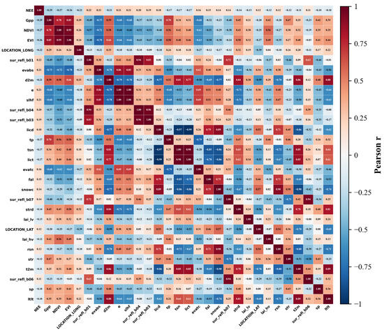
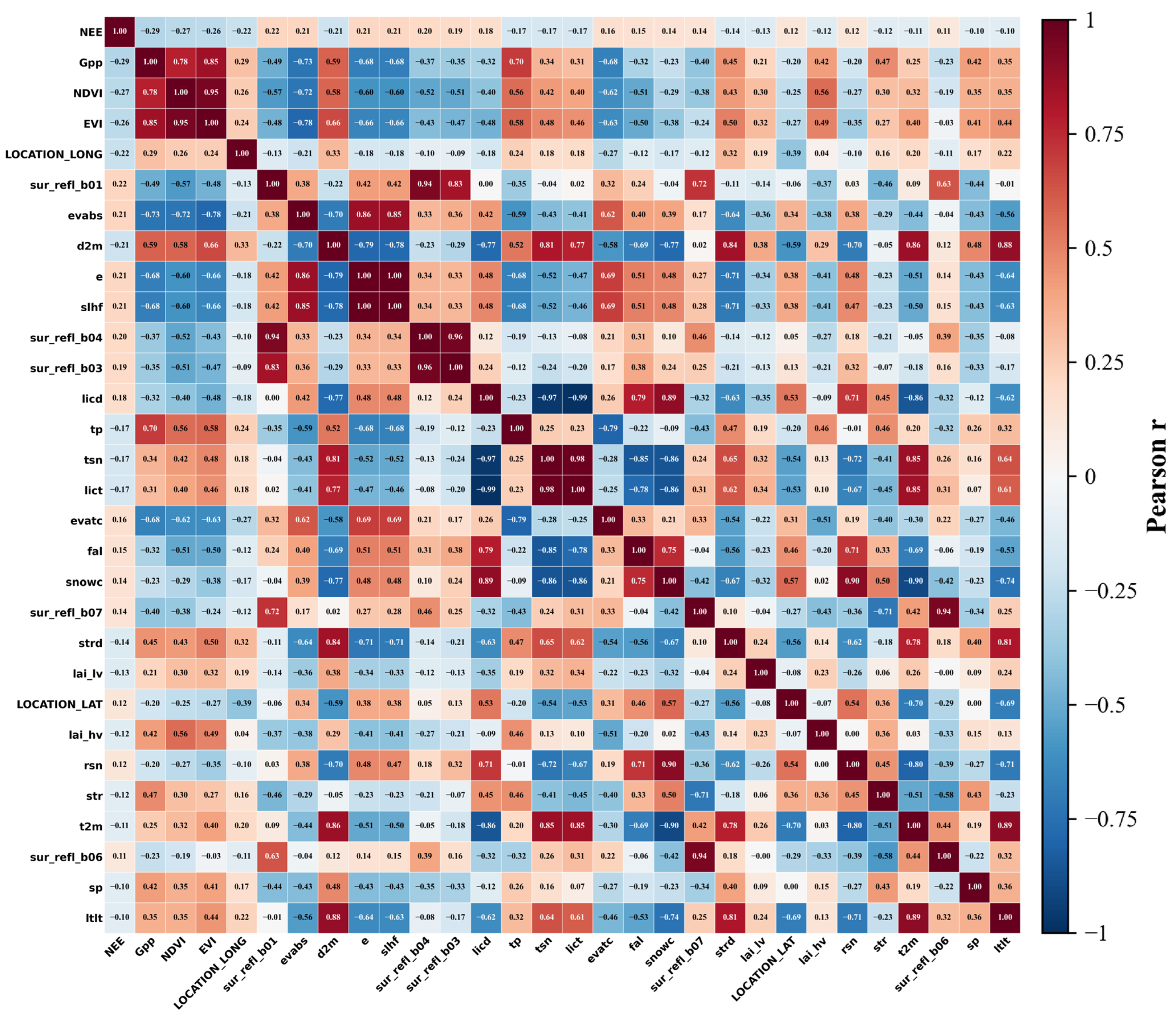
We initially compiled a candidate pool of 139 variables. A rigorous quality control procedure eliminated 13 features with excessive missing data, retaining 126 valid predictors (Table S1). These comprised 62 explicit environmental variables (e.g., ERA5 climate forcing, MODIS surface reflectance, and topographic metrics) and the 64-dimensional AlphaEarth embeddings (A00–A63). To mitigate multicollinearity and reduce the risk of overfitting, the 62 explicit variables were subjected to Pearson correlation analysis (Figure 1). Variables exhibiting weak linear associations with NEE (|r| < 0.1) were discarded. This screening removed 34 redundant predictors, yielding a refined subset of 28 core explicit features. This subset served as the input for our baseline inversion models (e.g., RF_CORR), providing a dimensionally reduced foundation for the historical NEE reconstruction.

Figure 1. Pearson correlation matrix between NEE and environmental covariates.

Notably, the 64 AlphaEarth embedding dimensions were explicitly excluded from the aforementioned correlation screening. Generated via deep representation learning, these embeddings function collectively as an indivisible holistic vector rather than independent physical measurements. They serve as integrated “environmental fingerprints” to overcome the limitations of conventional optical indices, such as NDVI saturation in high-biomass regions. For the 2017–2024 experimental period, we established an embedding-enhanced framework by directly concatenating these 64 dimensions with the 28 core explicit features. This combined configuration allowed us to formally quantify the information gain provided by high-dimensional foundation model features in improving global NEE inversion.

2.2.3. Model Selection

To capture the nonlinear relationships between environmental drivers and NEE, and to evaluate model robustness under high-dimensional feature settings, three representative tree-based ensemble algorithms were employed: Random Forest [16], LightGBM [17], and XGBoost [9]. Spanning both the bagging and boosting paradigms, these models offer complementary strengths in representing complex ecosystem dynamics. Prior to training, the spatiotemporally matched FLUXNET site–year observations were randomly partitioned into an 80% training set and a 20% independent test set. The former was utilized for model fitting, while the latter was reserved to assess generalization capability and explicitly monitor potential overfitting. To ensure rigorous inter-model comparability, all algorithms were trained under identical data partitions, fixed random seeds, and consistent feature configurations, with parallel computing enabled to optimize computational efficiency. All machine learning models, feature scaling, and data preprocessing were implemented in Python 3.10.

(1)

Random Forest

Random Forest was established as the baseline model owing to its proven efficacy in managing nonlinearities, complex interactions, and correlated predictors. The model was configured with an ensemble of 500 unconstrained decision trees. This extensive ensemble size was specifically selected to stabilize variance by averaging predictions across diverse feature subspaces—an essential mechanism when integrating high-dimensional remote-sensing embeddings.

(2)

LightGBM

LightGBM was selected as a representative gradient boosting framework. It was trained over 500 iterations with a learning rate of 0.05. To govern model complexity and ensure robust generalization, the maximum number of leaves per tree was capped at 31, alongside a strict constraint of at least 20 samples per leaf.

(3)

XGBoost

XGBoost was incorporated as a complementary boosting algorithm. To maintain structural comparability, the model was similarly configured with an ensemble of 500 trees and a learning rate of 0.05. Furthermore, the maximum tree depth was restricted to eight to prevent the development of overly complex interaction structures.

3. Results

3.1. Model Performance Evaluation

3.1.1. Accuracy Assessment of Different Models

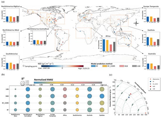
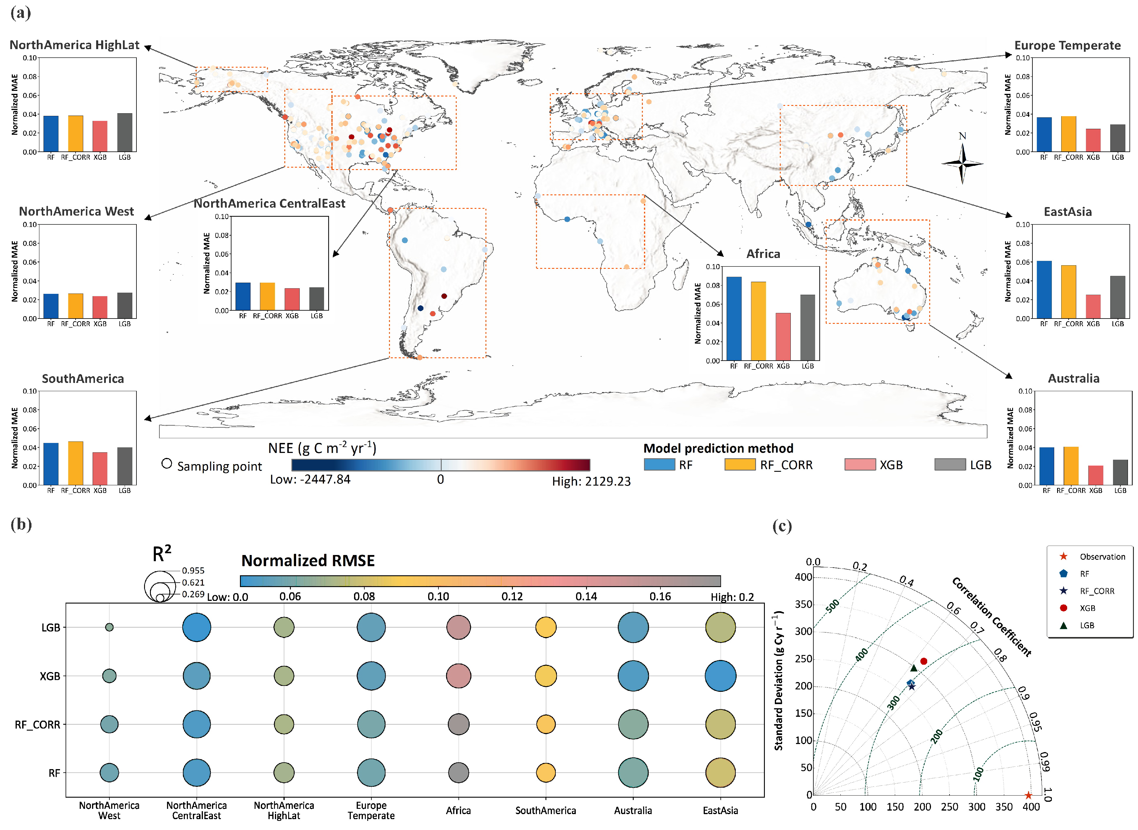
Statistical evaluation on an independent test dataset indicates that all three tree-based ensemble models—Random Forest, LightGBM, and XGBoost—capture the primary variability of global NEE. In the Taylor diagram (Figure 2c), predictions from all the models cluster around the observational reference. RF and RF_CORR achieve correlation coefficients closer to observations and standard deviations that better match the reference variance. Under the full-feature configuration, RF exhibits the highest overall stability with an R² of 0.52. XGBoost shows an R² of 0.49, while LightGBM displays greater dispersion in high-NEE ranges with an R² of 0.42.

Figure 2. Spatial distribution of sampling sites and regional performance of NEE inversion models. (a) Spatial distribution of sampling sites and regional model performance (Normalized MAE); (b) Cross-regional comparison of model R² and Normalized RMSE; (c) Taylor diagram of global performance.

Model performance varies when evaluated across eight major geographic regions (Table S5; Figure 2a,b). In Western North America, RF outperforms the boosting algorithms, achieving an R² of 0.42 compared to 0.31 for XGBoost. Conversely, in Temperate Europe and East Asia, XGBoost and LightGBM yield locally higher R² values, with XGBoost reaching an R² of 0.96 in East Asia, alongside lower Normalized MAE (Figure 2a).

The cross-regional bubble chart (Figure 2b) reveals that the R² and Normalized RMSE of XGBoost and LightGBM fluctuate across different regions. In contrast, RF maintains a more consistent error magnitude across both densely sampled areas and data-sparse domains, such as Africa and South America. Based on its highest aggregate accuracy and consistent cross-regional performance, the Random Forest model was selected to reconstruct the continuous 2000–2024 historical NEE baseline and to conduct the subsequent embedding-enhancement experiments.

3.1.2. Model Performance After Incorporating High-Dimensional Features

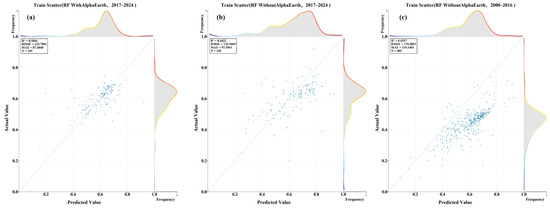
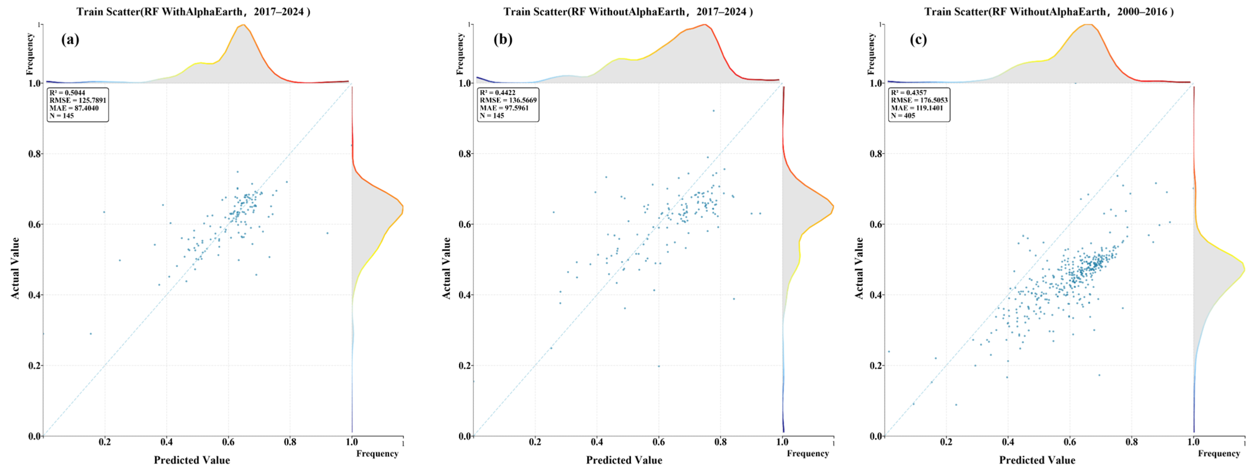
The performance gain provided by AlphaEarth embeddings was explicitly quantified using independent site–year samples from the FLUXNET network. During the 2017–2024 overlapping period, the baseline Random Forest model, driven solely by explicit variables, achieved an R² of 0.44 on the validation set (N = 145) (Figure 3b). Following the incorporation of AlphaEarth high-dimensional embedding features, model performance improved markedly, with the R² increasing to 0.50 (Figure 3a). Scatterplot comparisons demonstrate that the embedding-enhanced predictions exhibit tighter clustering around the 1:1 reference line, accompanied by reduced dispersion and fewer extreme departures. Furthermore, the marginal distributions following embedding inclusion reveal a narrower and more symmetric residual structure, indicating enhanced error control and reduced systematic bias.

Figure 3. Comparison of NEE inversion accuracy with and without high-dimensional embedding features. (a) Model performance enhanced with AlphaEarth embeddings for 2017–2024. (b) Baseline Random Forest model performance without AlphaEarth embeddings for 2017–2024. (c) Baseline Random Forest model performance without AlphaEarth embeddings for the historical period of 2000–2016.

The temporal reliability of the historical inversion prior to the availability of AlphaEarth data was verified through an independent evaluation of the baseline Random Forest model over the 2000–2016 period (Figure 3c). This evaluation on the historical test set (N = 405) yielded consistent and robust performance with an R² of 0.44. The comparable R² values between the historical period (0.44) and the 2017–2024 baseline (0.44) confirm that long-term interannual carbon dynamics derived from explicit variables remain stable and reliable even without the aid of foundation model features.

At the spatial scale, the broad global NEE structure is successfully reproduced by both feature configurations, characterized by a strong net carbon uptake in low latitudes and profound spatial heterogeneity across mid-to-high latitudes. The multi-year means for the 2017–2024 period further indicate that the embedding-enhanced inversions produce more continuous spatial gradients and a reduced extent of localized extremes. Overall, the inclusion of embeddings diminishes spatial fragmentation, yielding smoother and more internally consistent regional patterns through a stronger suppression of spatial noise.

3.1.3. Model Adaptability Across Spatial Domains

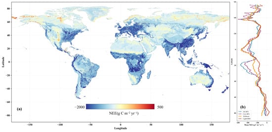
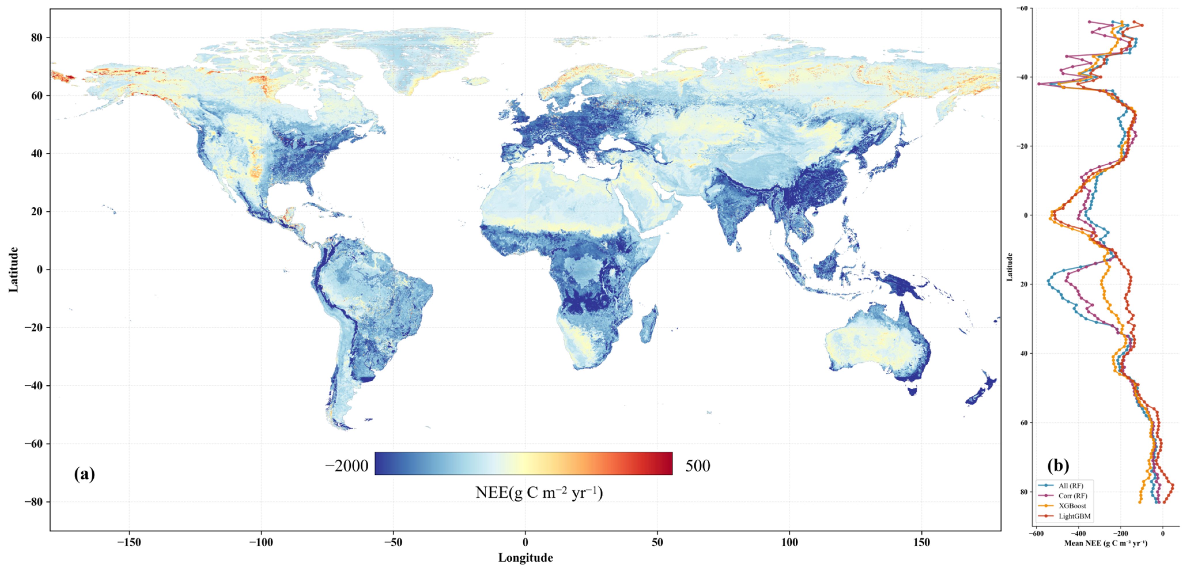
All three models successfully reproduce the macro-scale spatial distribution of global terrestrial NEE. As illustrated in Figure 4, low-latitude tropical ecosystems consistently exhibit strong net carbon uptake, whereas mid- and high-latitude regions display pronounced spatial heterogeneity. Under the full-feature configuration (integrating the high-dimensional remote-sensing embeddings), the RF model yields relatively continuous global latitudinal gradients, characterized by smooth meridional variation in NEE. Following correlation-based feature screening, RF preserves an overarching spatial macro-pattern but introduces sharper local gradients within specific mid- and high-latitude domains.

Figure 4. Spatial adaptability of NEE inversion models in 2023. (a) NEE inverted by the Random Forest model using the full feature set. (b) Latitudinal profiles of zonal mean NEE for the four models, used to assess model adaptability across latitude. Global NEE maps produced by different models for 2023 are provided in Supplementary Figures S1–S4.

XGBoost produces more pronounced localized high- and low-magnitude NEE patches, particularly across mid- to high-latitude Eurasia and topographically complex terrains. This indicates a heightened sensitivity to small-scale spatial variability and localized environmental forcings. By contrast, LightGBM exhibits steeper meridional contrasts at high latitudes, characterized by larger-amplitude fluctuations along zonal mean latitudinal transects.

Overall, while the models converge on large-scale spatial patterns, their divergence in spatial continuity and the strength of latitudinal variance highlights model-specific sensitivities to the underlying environmental heterogeneity of the global terrestrial biosphere.

3.2. Spatiotemporal Distribution of Global NEE

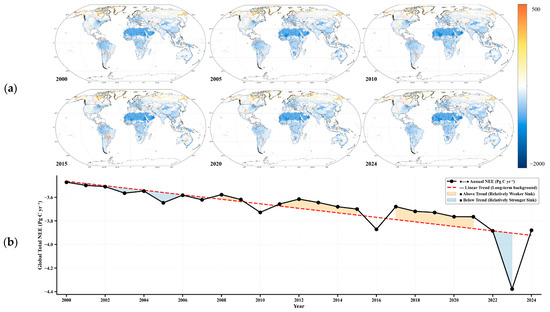
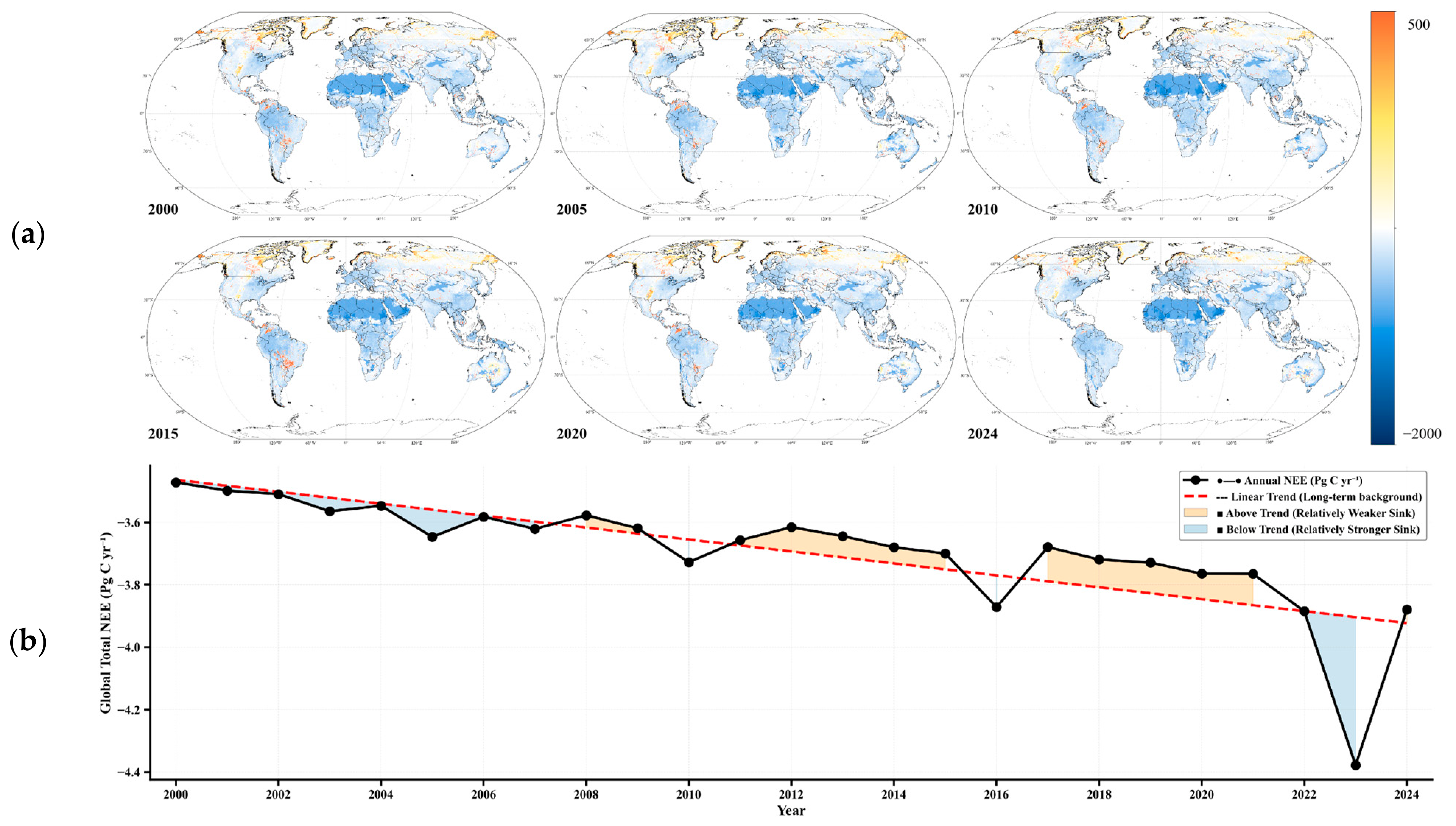
Based on the global terrestrial NEE inversion results for 2000–2024, the spatial distribution and interannual variability of NEE were systematically examined (Figure 5). Spatially, global NEE exhibits a persistent and pronounced latitudinal structure across the study period. Low-latitude tropical regions consistently show strongly negative NEE, concentrated in northern South America, central Africa, and Southeast Asia. Mid-latitude regions are characterized by moderately negative values, whereas high latitudes generally exhibit weaker net uptake, with localized transitions between negative and positive NEE.

Figure 5. Spatiotemporal evolution of global terrestrial NEE from 2000 to 2024. (a) Spatial distribution of annual terrestrial NEE for six representative years, illustrating long-term changes in global NEE patterns. (b) Time series of global annual total terrestrial NEE from 2000 to 2024, showing the long-term trend and interannual variability.

Across the time series, the large-scale spatial structure of global NEE remains highly consistent, with no evident shifts in the dominant patterns of carbon exchange. Comparisons among representative temporal milestones (2000, 2005, 2010, 2015, 2020, and 2024) confirm that the spatial locations of major carbon sink and weak sink regions are largely stable. Interannual differences manifest primarily as fluctuations in magnitude rather than structural reorganizations. Ultimately, low-latitude biomes continuously dominate the global net carbon sink, while mid- to high-latitude domains introduce greater spatial heterogeneity into the global carbon cycle.

Temporally, global annual terrestrial NEE remains negative over 2000–2024, with totals net uptake fluctuating between approximately −3.5 and −4.4 Pg C yr⁻¹. To characterize long-term dynamics, a linear trend was fitted to the interannual NEE time series to establish a baseline trajectory. Years with NEE values departures from this trajectory were subsequently classified as positive or negative anomalies.

During the first decade of the record, annual NEE values adhered closely to the baseline trend, indicating relatively constrained interannual variability. However, post-2010, the amplitude of these interannual fluctuations intensified, characterized by a higher frequency of strong negative anomalies (i.e., enhanced carbon sinks). In the latter portion of the record, a pronounced negative departure drove the global NEE toward its multi-decadal minimum (approximately −4.4 Pg C yr⁻¹), followed immediately by a rapid rebound toward the long-term baseline. Overall, interannual variability is characterized mainly by fluctuations around the fitted trend, whereas long-term change is expressed as gradual evolution captured by the trend itself.

3.3. Continental-Scale NEE Patterns

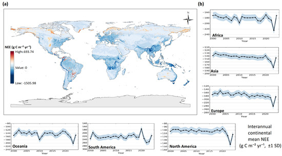
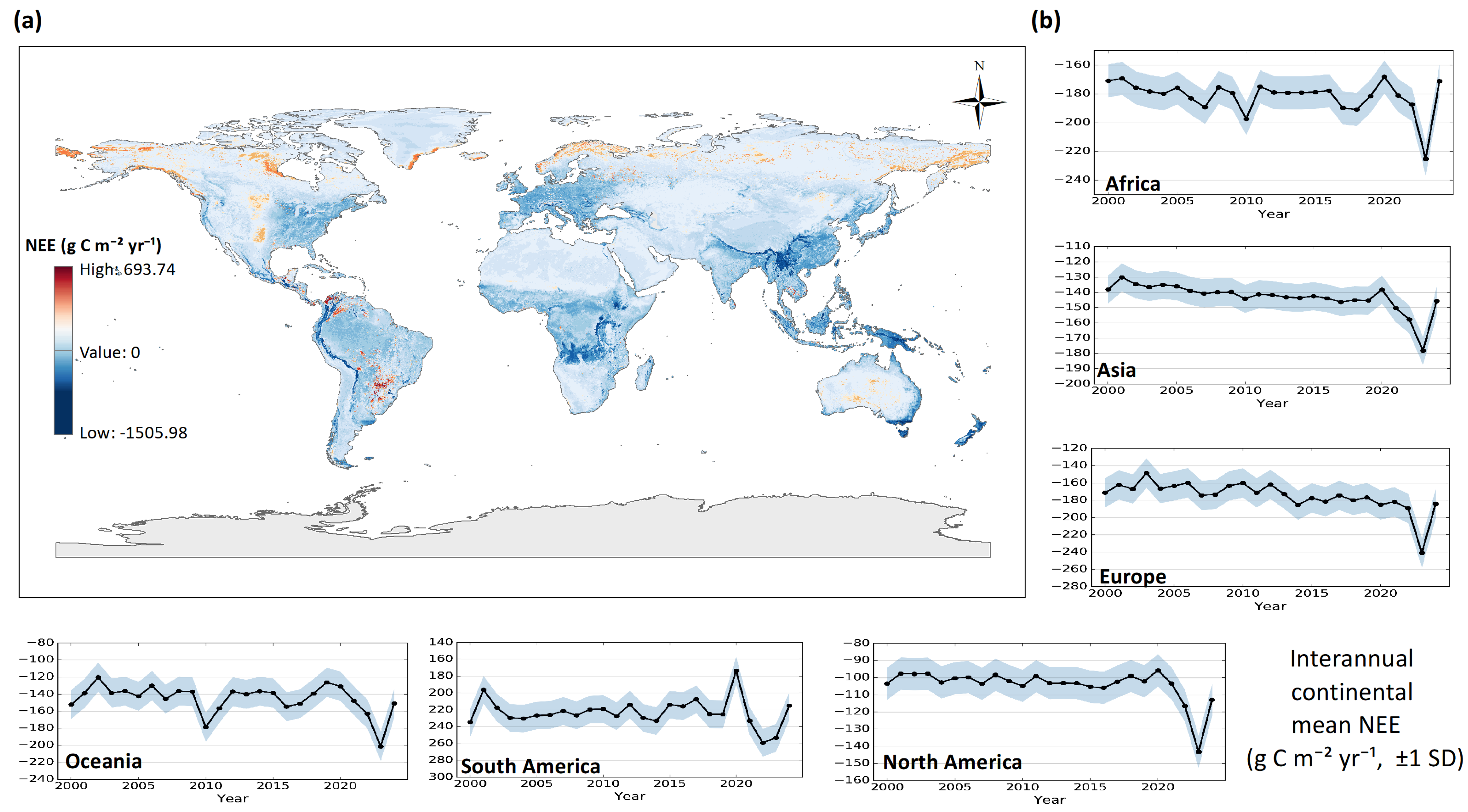
At the continental scale, global terrestrial NEE displays pronounced and persistent regional disparities (Figure 6). Multi-year means indicate stable differences in annual NEE contributions among continents. South America and Africa consistently exhibit the most robust net carbon uptake (i.e., highly negative NEE), together acting as the dominant drivers of the global terrestrial carbon sink. North America and Oceania show moderate sink capacities, whereas Europe and Asia display smaller absolute NEE magnitudes coupled with comparatively higher interannual variability. The corresponding annual totals for global and continental NEE are detailed in Table S2.

Figure 6. Spatial distribution and continental-scale characteristics of global terrestrial NEE. (a) Global map of predicted mean NEE at 0.1° resolution. (b) Interannual trends of continental mean NEE from 2000 to 2024.

From a latitudinal perspective, the major continental NEE contributions are densely concentrated in low- to mid-latitude regions, though the dominant functional bands vary geographically (Figure 6a). In South America and Africa, intense carbon sink zones are tightly coupled with equatorial and sub-equatorial domains, reflecting the persistent carbon sequestration capacity of tropical forests and woodlands. These low-latitude regions form spatially coherent, contiguous sink cores with limited fragmentation.

Conversely, the primary carbon sinks in North America and Eurasia are distributed across mid-latitude bands, corresponding largely to temperate forests and mixed-vegetation biomes. High-latitude areas generally show weaker absolute NEE values alongside elevated spatial heterogeneity. These areas are characterized by the localized coexistence of net-sink, near-neutral, and net-source patches, particularly across the boreal forest and tundra transition zones, resulting in a highly variable and attenuated contribution to the annual mean NEE. At the continental scale, terrestrial NEE displays pronounced and persistent regional contrasts (Figure 6b). The multi-year mean results reveal stable differences in both magnitude and variability among continents.

Overall, continental-scale NEE patterns are intrinsically regulated by the interplay between continental landmass extent and internal latitudinal biome distribution. Continents dominated by low-latitude ecosystems provide a stable, foundational baseline to the global NEE signal. In contrast, mid- and high-latitude landmasses exhibit amplified interannual fluctuations, evidenced by the broader variance envelopes in their temporal profiles. Despite differences in interannual volatility, the relative ranking of continental contributions to the global carbon sink remains remarkably stable from 2000 to 2024; interannual dynamics manifest predominantly as amplitude modulations rather than shifts in continental dominance.

4. Discussion

4.1. Spatiotemporal Consistency and Uncertainty of Global NEE Estimates

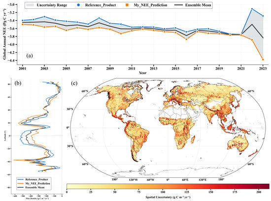
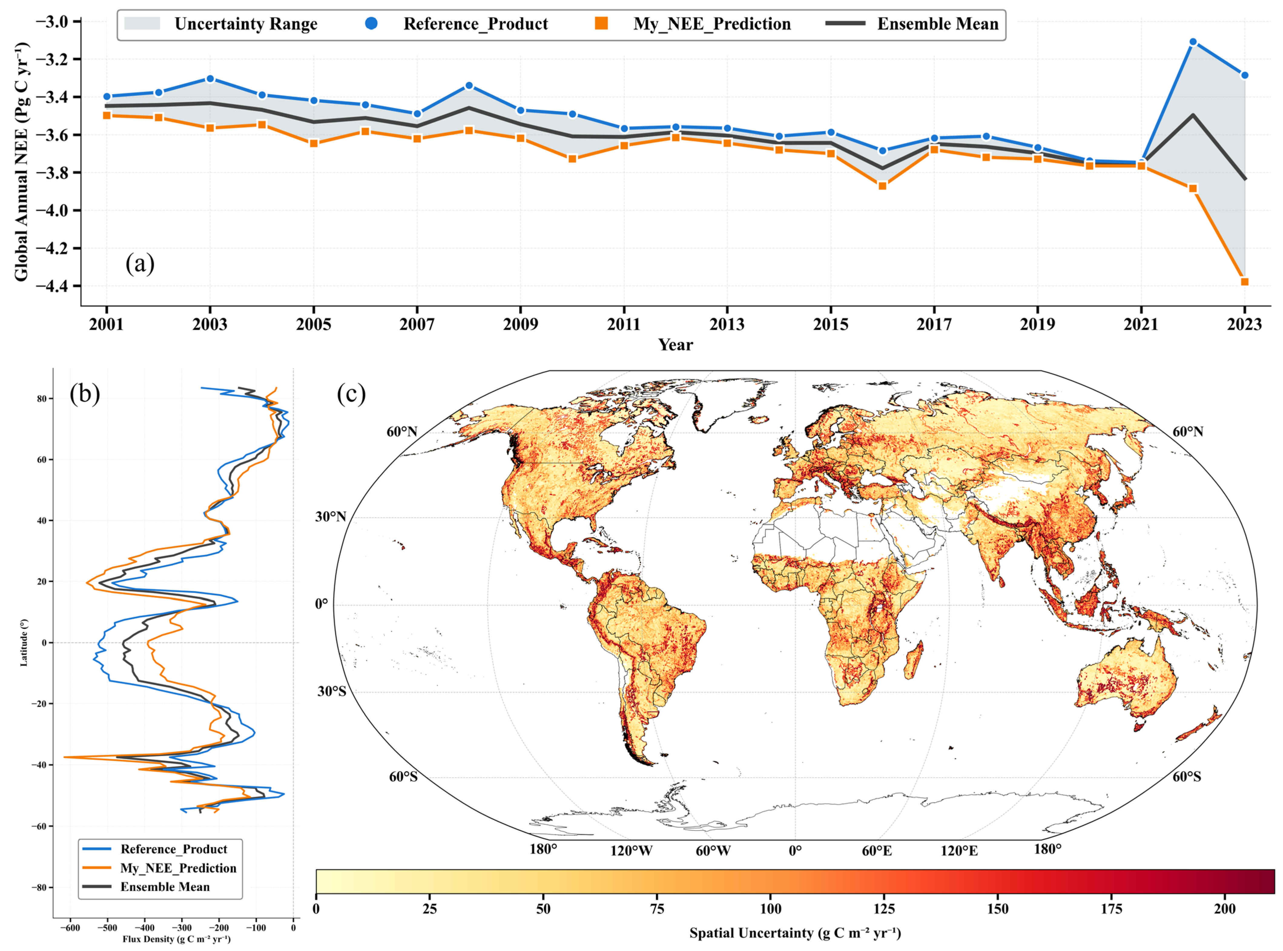
To evaluate the spatiotemporal consistency of the global NEE estimates produced in this study and to quantify associated uncertainties, multi-scale comparisons were conducted. The predicted global annual totals for 2001–2023 overlapping period were cross-examined against existing reference products and their ensemble mean (Figure 7). The evaluation framework deliberately emphasizes consistency across common diagnostic dimensions, rather than relying solely on pointwise agreement.

Figure 7. Consistency and uncertainty of global terrestrial NEE estimates. (a) Temporal evolution of global annual total NEE from 2001 to 2023 (Pg C yr⁻¹). The orange line represents NEE predicted in this study (My_NEE_Prediction), the blue line denotes the reference product [15], and the black solid line indicates the ensemble mean. The shaded gray area represents the estimated uncertainty range across products. (b) Latitudinal zonal mean distribution of NEE flux density (g C m⁻² yr⁻¹), comparing the predictions from this study with the reference product across latitude bands. (c) Spatial distribution of NEE estimation uncertainty, expressed as the standard deviation among products (g C m⁻² yr⁻¹), where darker (red) colors indicate higher uncertainty and larger inter-product discrepancies.

At the global annual total scale (Figure 7a), the NEE time series generated in this study demonstrates high consistency with both individual reference products and their ensemble mean, particularly regarding phase coherence and long-term background evolution. Global annual NEE remains persistently negative, varying within approximately −3.5 to −4.4 Pg C yr⁻¹, consistent with the magnitude reported in the Section 3. This agreement indicates that interannual variability derived from our machine learning-based inversion, which effectively integrates high-dimensional remote-sensing embeddings, is not subject to spurious drift; rather, it remains well-constrained within the variability envelope supported by existing global products. To further corroborate these temporal dynamics, a detailed year-by-year quantitative comparison of the global mean NEE flux density and total annual carbon budget between our predictions and the reference dataset is provided in Table S4. From the perspective of the global carbon budget, such consistency implies that the inferred source–sink status and its interannual fluctuations are broadly comparable across methodological frameworks.

Importantly, the inclusion of the ensemble mean and its associated uncertainty envelope enables deviations to be interpreted relative to inter-product spread. When predicted values fall within the uncertainty range, differences are more appropriately attributed to methodological diversity—data-driven approaches, process-based models, or hybrid products—rather than to systematic bias [3,13].

At the latitudinal scale (Figure 7b), the zonal mean NEE estimated in this study reproduces the characteristic meridional structure reported by recent global syntheses. It captures the pronounced net carbon uptake in the tropics and increasingly complex gradients toward mid and high latitudes. This latitudinal organization is widely regarded as a critical constraint on the physical plausibility of large-scale carbon flux estimates because it reflects the integrated effects of long-term radiation balance, thermal regimes, and moisture availability across climate zones. The successful recovery of this structure suggests that the model captures emergent, large-scale carbon exchange patterns rather than merely extrapolating from sparse flux observations [18,19].

Furthermore, zonal averaging highlights the scale dependence introduced by annual aggregation. Although aggregation suppresses short-term meteorological variability and site-level anomalies, the overarching meridional gradients remain governed by persistent land–atmosphere coupling processes operating on multi-year timescales. Consequently, this diagnostic emphasizes background structural consistency of carbon exchange rather than pointwise agreement at individual locations or in specific years, thereby providing a robust, complementary assessment of large-scale realism relative to site-based validation [20,21].

Spatial uncertainty patterns, quantified as the pixel-scale standard deviation across the compared products (Figure 7c), exhibit pronounced spatial heterogeneity, characterized by adjacent regions of high and low uncertainty. This behavior aligns with prior global carbon flux assessments, which document amplified inter-product divergence in regions subject to multiple interacting environmental constraints, particularly water limitation, energy limitation, and disturbance [13,17,22]. Accordingly, these spatial uncertainty maps indicate not only the magnitude of disagreement but also where additional independent constraints may be most effective for uncertainty reduction [8,13].

4.2. Plausibility of Interannual NEE Anomalies

The pronounced interannual fluctuation observed in the global NEE time series during 2022–2023 (Figure 8) represents a prominent dynamic that warrants rigorous validation to preclude artifacts of model instability or error amplification. Accordingly, the physical plausibility of this anomaly was assessed using independent contextual evidence, cross-scale consistency diagnostics, and model interpretability frameworks.

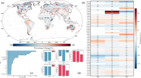
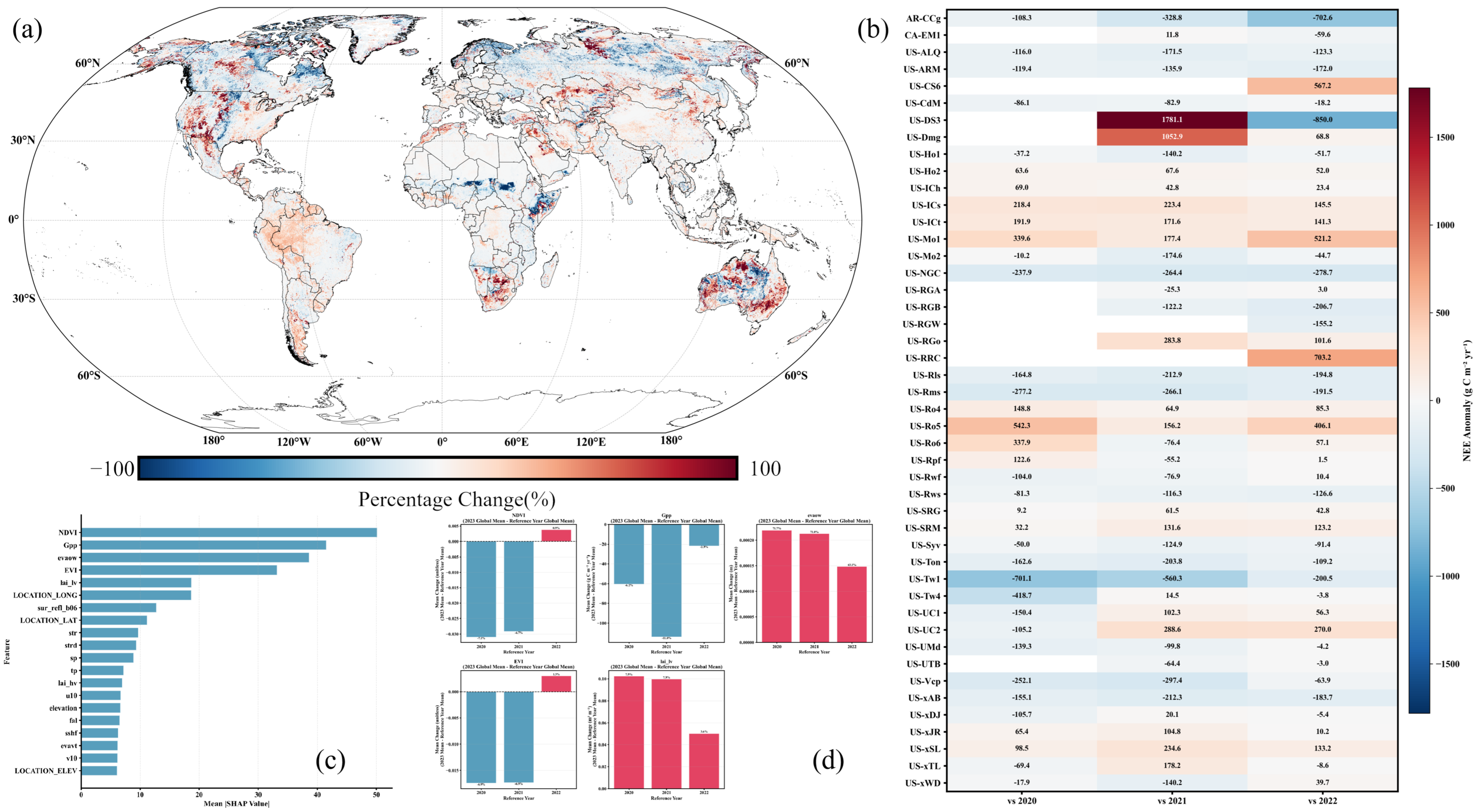
Figure 8. Spatiotemporal anomalies of global terrestrial NEE in 2023 and attribution of dominant drivers. (a) Global spatial distribution of NEE anomalies in 2023 relative to 2022. (b) Site-scale consistency assessment based on FLUXNET observations, showing NEE anomalies in 2023 relative to the multi-year mean of 2020–2022. (c) Feature importance ranking derived from SHapley Additive exPlanations (SHAP), quantifying the relative contributions of environmental drivers to model predictions. (d) Mean changes in the five dominant drivers (NDVI, GPP, evaow, EVI, and lai_lv) in 2023 relative to different reference years (2020–2022).

At the 0.1° spatial scale, the NEE anomalies in 2023 relative to 2022 exhibit coherent geographic organization rather than random pixel-scale noise (Figure 8a). These anomalies manifest as expansive, spatially contiguous patches with consistent directional signs across broad ecoregions. Such spatial coherence is widely recognized in carbon-cycle studies as a hallmark of genuine, large-scale ecosystem responses to climatic forcings, making it highly unlikely that the signal stems from localized noise or non-physical error propagation during the inversion process. Similar spatial contiguity metrics are frequently employed as fundamental credibility indicators in the comparative evaluation of global carbon flux products [7,12].

At the site scale, independent FLUXNET observations provide crucial constraints on the 2023 NEE anomaly (Figure 8b). Relative to the multi-year baseline (2020–2022), multiple eddy covariance sites exhibit anomaly directions and magnitudes that align robustly with our model-derived estimates. Although the response amplitude varies among sites, no systematic sign reversal is observed, indicating that the anomaly does not arise from pervasive site-level mismatch. This site-level consistency is further supported by the global-scale comparison shown in Figure 7a, where the 2022–2023 deviation in the predicted global annual NEE remains well within the uncertainty envelope defined by existing reference products and their ensemble mean. The coherence between local site anomalies and the global annual signal suggests that the 2023 anomaly reflects a scale-consistent response rather than noise amplification during spatial aggregation.

Consistency in anomaly sign between site observations, gridded inversion outputs, and global annual totals is widely regarded as a key credibility criterion for data-driven carbon flux estimates, particularly for assessing anomalous years see refs [4,7]. Together, these cross-scale agreements support the interpretation that the 2023 NEE anomaly represents a physically plausible ecosystem response rather than an artifact of model instability.

From an internal interpretability perspective, SHAP-based attribution analysis indicates that the anomalous 2023 NEE estimates are primarily driven by variables intrinsically linked to vegetation phenology and photosynthetic capacity, rather than spurious correlations (Figure 8c). Among the integrated high-dimensional remote-sensing embeddings, variables such as NDVI, GPP, evapotranspiration-related variables, EVI, and LAI emerge as the overwhelmingly dominant contributors. This hierarchical ranking demonstrates that the modeled carbon response is governed by ecologically meaningful biophysical drivers rather than weakly related auxiliary predictors, ensuring that the anomaly carries a discernible, process-based ecological signature [23].

Finally, a temporal examination of the top-ranked drivers shows consistent shifts in 2023 across multiple reference years (2020–2022), maintaining aligned anomaly directions and physically plausible magnitudes regardless of the selected baselines (Figure 8d). This multi-baseline agreement implies that the inferred NEE anomaly is not sensitive to baseline selection but instead reflects a coordinated multi-variable response. Collectively, these cross-scale and interpretable diagnostics support interpreting the 2023 NEE anomaly as a plausible ecosystem response under specific environmental conditions, rather than as a manifestation of model instability.

4.3. Structural Regulation of Interannual NEE Stability by Land Cover Types

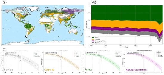
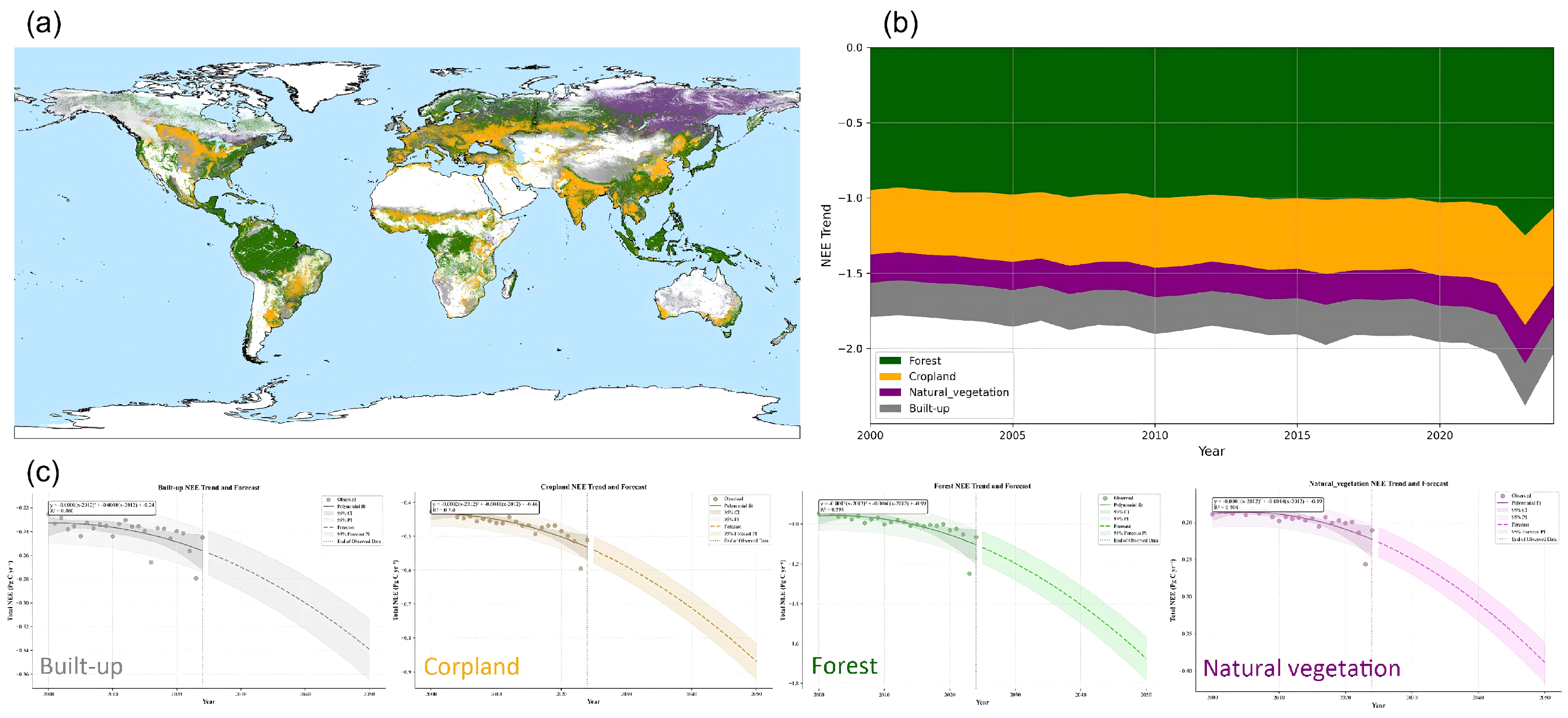
The long-term global NEE pattern is not attributable to a single ecosystem type; instead, it reflects differentiated contributions of multiple land cover classes. Under multi-year mean conditions, the most spatially continuous and strongly negative NEE occurs predominantly within tropical forests and the mid- to high-latitude forest belts, forming coherent carbon sink cores (Figure 9a). In contrast, croplands and non-forest vegetation types exhibit more fragmented and region-dependent NEE patterns, with localized highs and lows more tightly coupled to climatic gradients and land-use intensity. This contrast suggests a relatively stable functional partitioning: forests provide the spatial backbone of the global carbon sink, whereas non-forest systems more readily express sensitivity to environmental variability. Land cover-specific NEE statistics supporting these patterns are reported in Table S3.

Figure 9. Land cover-specific spatial patterns and temporal contributions to global terrestrial NEE (2000–2023). (a) Mean global NEE distribution aggregated by major land cover types over 2000–2023, where green, orange, purple, and gray denote forest, cropland, natural vegetation, and built-up areas, respectively. (b) Decomposition of global NEE into land cover–specific contributions, showing the stacked-area trend of each land cover type from 2000 to 2023. (c) Long-term NEE trends and forecasts for the four land cover types (built-up, cropland, forest, and natural vegetation), with shaded envelopes indicating the prediction uncertainty range.

Temporal aggregation of land cover-specific contributions further corroborates this spatial interpretation (Figure 9b). Forests consistently constitute the dominant negative component of global annual NEE, thereby stabilizing the long-term baseline. Non-forest (e.g., savannas, shrublands, and grasslands) contributes less in terms of absolute magnitude but exhibits stronger interannual variability, thus plays a disproportionate role in modulating year-to-year fluctuations. Croplands contribute relatively small absolute magnitudes but show discernible variability in certain years, indicating that their influence, although secondary, remains ecologically non-negligible. Similar “stable core–variable modulation” structures have been repeatedly reported in global carbon flux inversion and ensemble studies, and are widely interpreted as manifestations of ecosystem-type differentiation at the global scale [7,12].

Trend decomposition by land cover type further reveals divergent trajectories among major ecosystem classes. Forest NEE demonstrates a smooth, persistent shift toward more negative values over the study period, suggesting a gradual, long-term strengthening of carbon uptake capacity. This behavior aligns seamlessly with recent syntheses highlighting the sustained contribution of intact forests to the global terrestrial carbon sink under contemporary climate forcings [24,25]. Natural vegetation exhibits a broadly similar long-term tendency but with greater nonlinearity and wider uncertainty envelopes, indicating higher interannual elasticity and sensitivity to climate variability. This pattern accords with evidence that non-forest and semi-natural ecosystems disproportionately amplify year-to-year variability in the land carbon sink, particularly under hydroclimatic fluctuations [26,27]. Conversely, cropland NEE trends are comparatively muted, displaying only modest long-term changes with indications of localized acceleration in recent years. This constrained signal is consistent with the strong influence of management practices and other anthropogenic controls, which tend to constrain variability relative to natural ecosystems [28,29].

Ultimately, these consistent patterns across spatial distributions magnitude decompositions, and temporal trends confirm that forests function as the foundational core of the global terrestrial carbon sink, while natural vegetation acts as the primary interannual modulator. The ability of the proposed remote-sensing framework to capture this structural regulation—without overextending into unconstrained mechanistic attribution—highlights its robustness. Consequently, land cover type emerges as a critical, organizing dimension for subsequent attribution analyses targeting anomalous climatic years or priority ecological regions.

4.4. Mechanisms of Information Gain from High-Dimensional Embedding Features in Global NEE Inversion

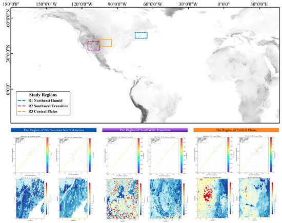
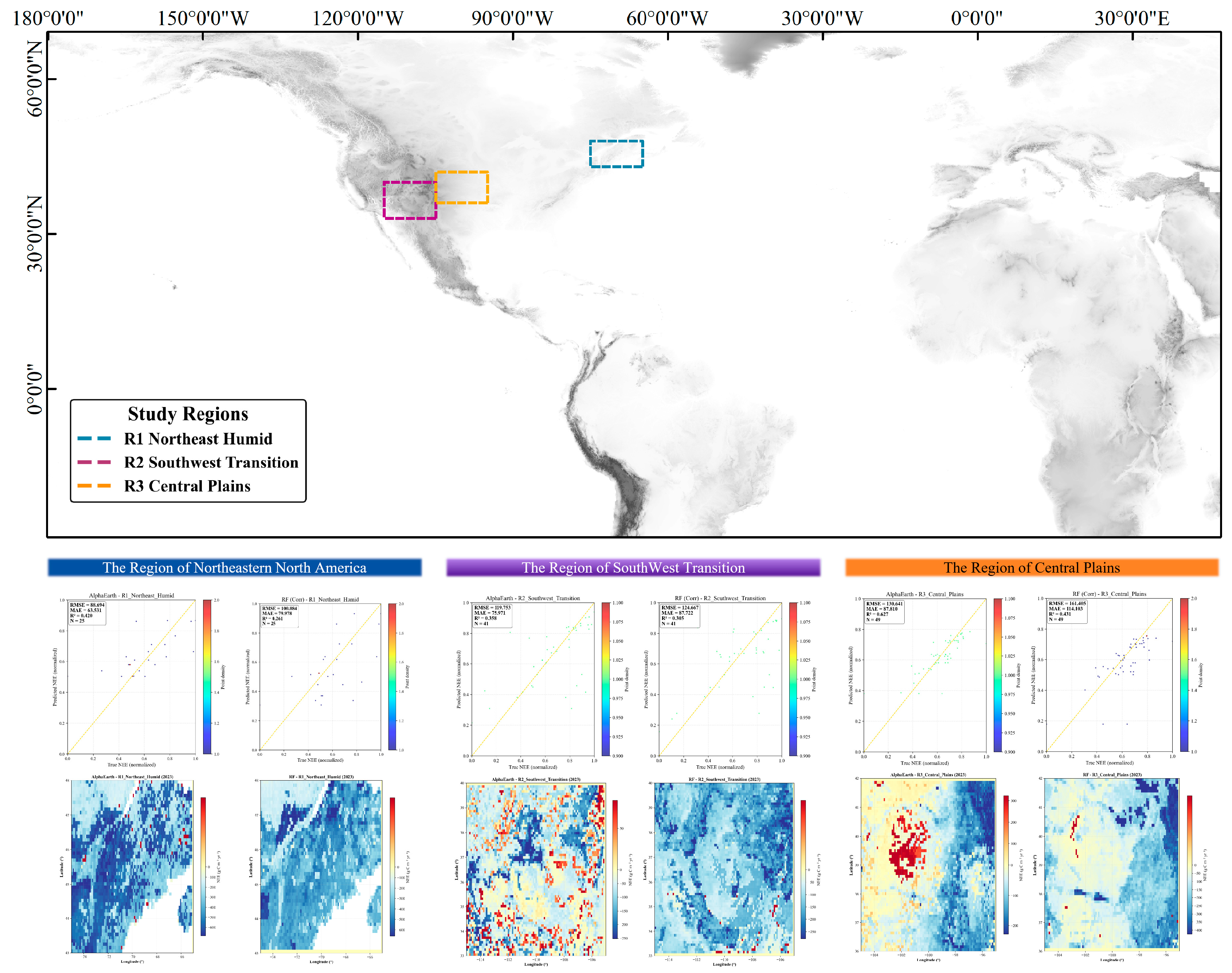
To further elucidate the specific role of high-dimensional embedding features, comparative analyses were conducted across three representative regions (R1–R3) in North America with contrasting ecological structures and climatic regimes (Figure 10). A detailed quantitative comparison of model performance metrics with and without AlphaEarth embeddings across these sub-regions is presented in Table S6. The results indicate that the information gain afforded by AlphaEarth embeddings is spatially heterogeneous and is strongly conditioned by ecosystem complexity, climatic stability, and the degree of environmental heterogeneity.

Figure 10. Selection of representative regions and comparison of NEE inversion performance across contrasting climate–ecosystem zones.

In the humid northeastern North America–eastern Canada region (R1), the ecosystem structure is comparatively homogeneous, dominated by forests and mixed woodlands experiencing relatively stable climatic conditions and limited interannual variability. Previous studies suggest that NEE variability in humid forest ecosystems is primarily regulated by radiation, temperature, and phenological dynamics, resulting in comparatively stable driver–response relationships [30,31]. Consistent with this expectation, baseline models utilizing only explicit meteorological variables and conventional remote-sensing indices reproduce interannual NEE dynamics with reasonable fidelity in R1. However, the incorporation of high-dimensional embedding features further reduces error dispersion and improves interannual consistency. This indicates that in structurally simple and climatically stable regions, embeddings mainly enhance performance by compressing multi-source information and suppressing redundancy and noise rather than by altering the dominant response structure. This behavior is consistent with evidence that multi-source integration primarily improves the stability of carbon flux estimates in such ecosystems [12].

By contrast, the information gain derived from the embedding features is substantially larger in the semi-arid to arid transition zone of the southwestern United States (R2). Ecosystems in this region are acutely sensitive to water availability, exhibit large interannual NEE variability, and may shift in dominant limiting factors across years. Semi-arid and transitional systems are known to contribute disproportionately to global interannual carbon sink variability and remain among the most challenging regions for conventional modeling approaches [26,27]. In R2, models lacking embeddings exhibit persistent systematic biases and heightened sensitivity to extreme years and local anomalies. Following the inclusion of the embeddings, interannual fluctuations are more tightly constrained, suggesting that embeddings implicitly integrate information on vegetation structure, moisture stress, and environmental context across optical, radar, topographic, and climatic domains. In doing so, they compensate for the limitations of individual explicit variables in capturing nonlinear couplings among water stress, vegetation dynamics, and carbon exchange. This interpretation aligns with evidence that carbon cycle responses under extreme or transitional conditions are governed by profound nonlinearities and multi-factor interactions [17,22].

In the central North American plains (R3), where eddy covariance flux-site density is low and sample representativeness is limited, the advantages of high-dimensional embeddings are less consistently expressed. Within this region, inversion outcomes under alternative feature configurations display greater instability, indicating that under sample-limited conditions the information encoded in a high-dimensional feature space may not be reliably learned. This finding corroborates previous studies demonstrating that high-dimensional predictors can inadvertently introduce additional uncertainty when the available training sample size is insufficient to properly constrain the feature space [32].

Taken together, these regional comparisons elucidate that AlphaEarth embeddings do not merely replace traditional explicit variables; rather, they reorganize the predictor space to provide a more holistic representation of complex environmental states. In climatically stable regions, their primary contribution lies in noise suppression and consistency enhancement. In transitional and water-limited regions, they improve representation of nonlinear and tightly coupled eco-hydrological processes. Conversely, in sample-constrained regions, their benefit appears limited. This context dependence suggests that high-dimensional embeddings are most effective when used as complementary enhancements rather than as standalone substitutes, and their value is likely to increase with improving observation density and data availability.

4.5. Interpretable Contributions of Key Drivers to NEE Inversion in the Random Forest Model

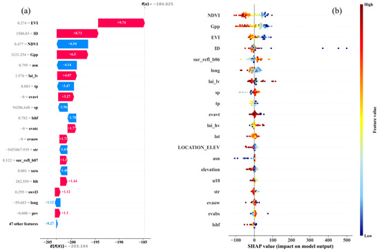
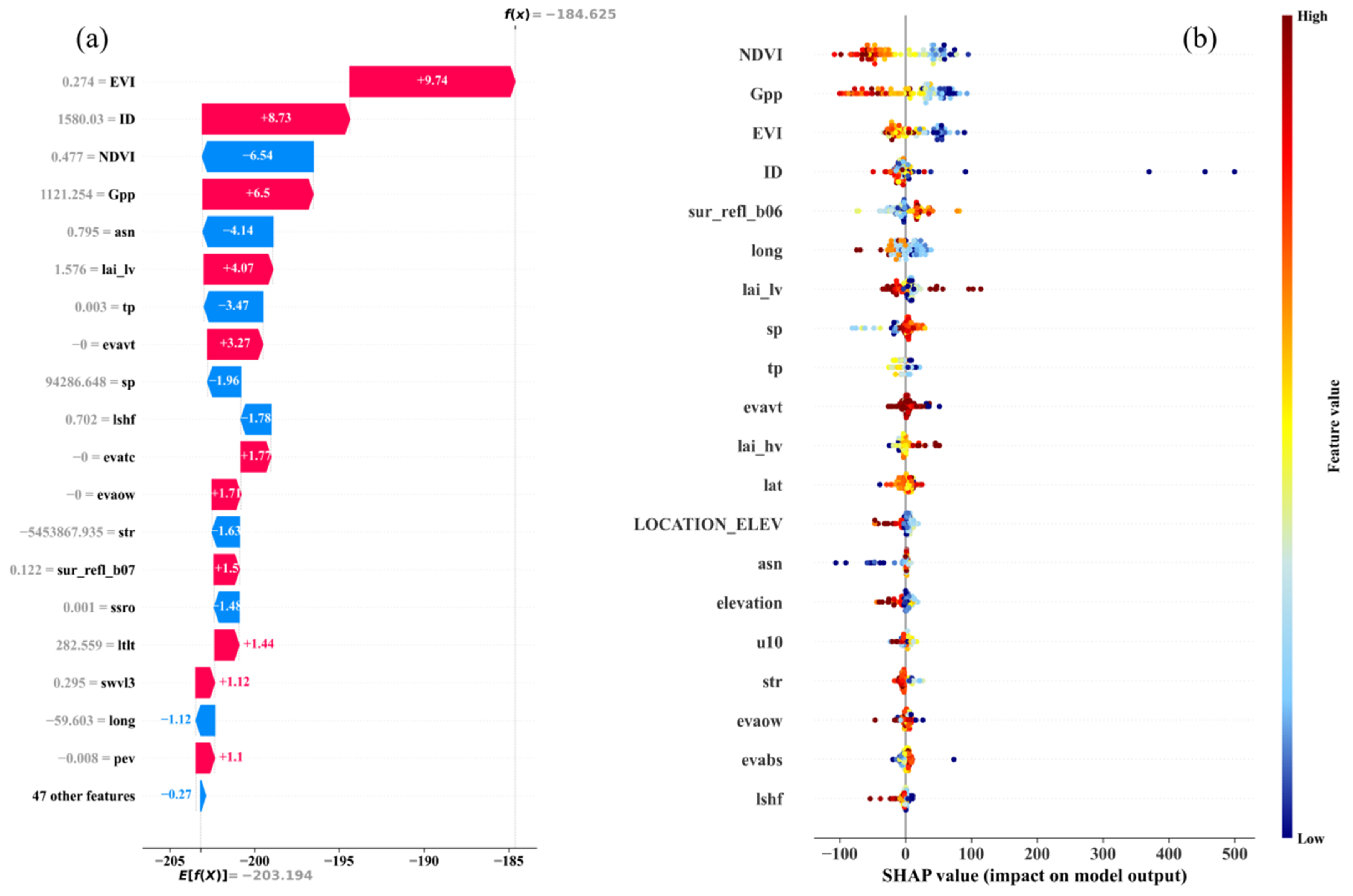
The model responses to the high-dimensional environmental drivers exhibit pronounced heterogeneity at both the individual sample level and in aggregate statistics. SHAP-based interpretability analysis reveals that global NEE predictions are not dominated by a single predictor; rather, they emerge from the structured, joint influence of remote-sensing-derived vegetation indices and variables related to carbon exchange.

At the individual sample level (Figure 11a), vegetation and productivity proxies such as EVI, GPP, and NDVI consistently exhibit the largest absolute SHAP contributions. This indicates that vegetation activity and productivity are the primary determinants of both the direction and magnitude of NEE deviations under specific environmental conditions. By contrast, most meteorological variables exert comparatively smaller influences at the single sample level, functioning predominantly as environmental modulators of the dominant, vegetation-driven signal rather than as primary controls.

Figure 11. SHAP-based interpretation of the NEE inversion model. (a) Local SHAP attribution for an individual prediction. (b) Global feature importance and impact patterns derived from SHAP values.

Across the full global sample distribution (Figure 11b), NDVI, GPP, and EVI display clear “high-value–high-impact” trajectories, whereby larger feature values are systematically associated with more negative SHAP contributions (i.e., corresponding to enhanced net carbon uptake). The overriding dominance of these high-dimensional vegetation state and productivity indicators aligns with recent data-driven syntheses. These studies demonstrate that photosynthetic activity and canopy development exert primary control over large-scale carbon exchange when models are trained to learn process-relevant signals rather than relying on spatial proxies. Specifically, advances in Earth system machine learning highlight that models capable of resolving fine-scale ecosystem productivity gradients exhibit stable, monotonic responses to vegetation-related predictors across biomes, reflecting genuine functional relationships rather than sampling artifacts [33,34]. Consequently, the coherent SHAP response patterns observed here therefore indicate that the model captures structurally meaningful linkages between ecosystem productivity and carbon exchange at the global scale.

Crucially, explicit geographic variables (such as longitude, latitude, and elevation) yield show SHAP contributions clustered near zero. This indicates that spatial position acts mainly as a passive background constraint rather than as a direct determinant of NEE magnitude or sign. This behavior provides compelling evidence that the model does not exploit spatial coordinates as surrogate predictors, but instead derives predictive skill from environmentally interpretable drivers. Previous critical evaluations of machine learning applications in carbon cycle research emphasize that limiting dependence on spatial location is critical for avoiding spurious skill and ensuring physically meaningful generalization, particularly under extrapolation to anomalous years or data-sparse regions [33,35]. Therefore, the attenuated SHAP influence of spatial variables observed here is therefore indicative of a model structure that prioritizes ecological signal learning over spatial autocorrelation.

Furthermore, meteorological and energy-related variables exhibit more dispersed SHAP distributions, with both positive and negative contributions across samples. This pattern reflects the conditional nature of their influence on NEE, with effect direction varying according to ecosystem state and environmental context. Such context-dependent behavior is consistent with evidence that interannual variability in terrestrial carbon uptake is strongly regulated by hydroclimatic constraints, whereby soil moisture availability and land–atmosphere feedbacks can amplify or offset the apparent effects of temperature and atmospheric demand under regional background conditions [36]. Additionally, because carbon cycle responses are often disproportionately shaped by spatiotemporally coherent extremes rather than mean climate states, meteorological drivers naturally exert bidirectional influences depending on whether these anomalies force ecosystems into stress-induced carbon emission or recovery-driven uptake regimes [21].

Overall, the SHAP analysis corroborates that the high-dimensional NEE predictions are fundamentally controlled primarily by vegetation state and productivity-related variables, while meteorological and spatial factors provide critical contextual modulation. The robust consistency of these driver hierarchies across both local and global scales confirms that the inversion model captures ecologically coherent response structures rather than statistical artifacts. This interpretability seamlessly reinforces earlier macro-scale interpretations of anomalous-year behaviors and land cover-specific structural regulations.

5. Conclusions

This study integrates 0.1° high-dimensional remote-sensing embeddings (AlphaEarth) with ensemble machine learning framework to systematically quantify the spatiotemporal distribution and interannual dynamics of global terrestrial NEE. The principal findings are summarized as follows.

First, the incorporation of high-dimensional embedding features substantially enhances the stability and spatial consistency of global NEE inversion. Operating under identical model architectures, training samples, and parameterizations, these embeddings effectively suppress spatial noise and spurious localized gradients, providing a superior representation of integrated land surface states across complex environments. Compared to conventional feature spaces reliant on explicit climatic variables and traditional vegetation indices, this embedding-based approach offers a fundamentally more robust, data-driven foundation for large-scale carbon flux estimation, highlighting the critical role of feature representation in constraining inversion performance.

Second, while global terrestrial ecosystems maintained a persistent net carbon sink state over the 25-year study period, the intensity of this sink exhibited a phased weakening. The global aggregated annual mean NEE remained definitively negative throughout 2000–2024, dictating continued net carbon removal from the atmosphere. However, long-term interannual trajectory analysis reveals a gradual reduction in the absolute magnitude of this global sink post-2010. This trend signifies a weakening of carbon assimilation capacity rather than a wholesale transition to a net carbon source, emphasizing the critical need to distinguish between shifting sink intensities and absolute source–sink reversals when diagnosing long-term carbon cycle dynamics.

Third, the interannual variability of the terrestrial carbon sink displays pronounced asymmetry and strong ecosystem dependence. Against the backdrop of a persistent baseline sink, anomalous years characterized by diminished sink capacity tend to manifest abruptly (often driven by climate extremes), whereas subsequent recoveries in sink strength develop more gradually. Furthermore, these dynamics are highly stratified by ecosystem type: intact forest biomes function as robust and relatively stable carbon sinks; non-forest natural vegetation (e.g., grasslands and savannas) exhibits weaker but highly volatile sink behavior that largely dictates global interannual variability; and croplands display complex, secondary responses modulated jointly by climatic forcings and anthropogenic management.

In summary, by augmenting data-driven inversions with high-dimensional remote-sensing embedding, this study delivers a robust quantitative characterization of the long-term state, phased trajectory, and ecosystem-specific variability of global terrestrial NEE. These findings strengthen the empirical foundation for deciphering terrestrial carbon source–sink dynamics under accelerating climate change, ultimately informing more accurate future assessments of global carbon–climate feedback mechanisms.

References

- Baldocchi, D. Assessing the eddy covariance technique for evaluating carbon dioxide exchange rates of ecosystems: Past, present and future. Glob. Change Biol. 2003, 9, 479–492. [Google Scholar] [CrossRef] [Scilit]
- IPCC. Climate Change 2013: The Physical Science Basis. Contribution of Working Group I to the Fifth Assessment Report of the Intergovernmental Panel on Climate Change; Cambridge University Press: Cambridge, UK; New York, NY, USA, 2013. [Google Scholar]
- Friedlingstein, P.; O’Sullivan, M.; Jones, M.W.; Andrew, R.M.; Bakker, D.C.E.; Hauck, J.; Landschützer, P.; Le Quéré, C.; Peters, G.P.; Peters, W.; et al. Global Carbon Budget 2022. Earth Syst. Sci. Data 2022, 14, 4811–4900. [Google Scholar] [CrossRef] [Scilit]
- Piao, S.; Liu, Z.; Wang, T.; Peng, S.; Ciais, P.; Huang, M.; Wang, X. Weakening temperature control on the interannual variations of spring carbon uptake across northern lands. Nat. Clim. Change 2017, 7, 359–363. [Google Scholar] [CrossRef] [Scilit]
- Sitch, S.; Friedlingstein, P.; Gruber, N.; Jones, S.D.; Murray-Tortarolo, G.; Ahlström, A.; Doney, S.C.; Graven, H.; Heinze, C.; Huntingford, C.; et al. Recent trends and drivers of regional sources and sinks of carbon dioxide. Biogeosciences 2015, 12, 653–679. [Google Scholar] [CrossRef] [Scilit]
- Yu, G.; Fu, Y.; Sun, X.; Wen, X.; Zhang, L. Recent progress and future directions of ChinaFLUX. Sci. China Ser. D Earth Sci. 2006, 49, 1–23. [Google Scholar] [CrossRef] [Scilit]
- Tramontana, G.; Jung, M.; Schwalm, C.R.; Ichii, K.; Camps-Valls, G.; Ráduly, B.; Reichstein, M.; Arain, M.A.; Cescatti, A.; Kiely, G.; et al. Predicting carbon dioxide and energy fluxes across global FLUXNET sites with regression algorithms. Biogeosciences 2016, 13, 4291–4313. [Google Scholar] [CrossRef] [Scilit]
- Baldocchi, D.; Falge, E.; Gu, L.; Olson, R.; Hollinger, D.; Running, S.; Anthoni, P.; Bernhofer, C.; Davis, K.; Evans, R.; et al. FLUXNET: A new tool to study the temporal and spatial variability of ecosystem–scale carbon dioxide, water vapor, and energy flux densities. Bull. Am. Meteorol. Soc. 2001, 82, 2415–2434. [Google Scholar]
- Chen, T.; Guestrin, C. XGBoost: A scalable tree boosting system. In Proceedings of the 22nd ACM SIGKDD International Conference on Knowledge Discovery and Data Mining, San Francisco, CA, USA, 13–17 August 2016; ACM: New York, NY, USA, 2016; pp. 785–794. [Google Scholar] [CrossRef] [Scilit]
- Ke, G.; Meng, Q.; Finley, T.; Wang, T.; Chen, W.; Ma, W.; Ye, Q.; Liu, T.-Y. LightGBM: A highly efficient gradient boosting decision tree. In Advances in Neural Information Processing Systems 30 (NeurIPS 2017); Curran Associates, Inc.: Red Hook, NY, USA, 2017; pp. 3146–3154. [Google Scholar]
- Brown, C.F.; Kazmierski, M.R.; Pasquarella, V.J.; Rucklidge, W.J.; Samsikova, M.; Zhang, C.; Shelhamer, E.; Lahera, E.; Wiles, O.; Ilyushchenko, S.; et al. AlphaEarth foundations: An embedding field model for accurate and efficient global mapping from sparse label data. arXiv 2025, arXiv:2507.22291. [Google Scholar] [CrossRef] [Scilit]
- Jung, M.; Reichstein, M.; Margolis, H.A.; Cescatti, A.; Richardson, A.D.; Arain, M.A.; Arneth, A.; Bernhofer, C.; Bonal, D.; Chen, J.; et al. Global patterns of land–atmosphere fluxes of carbon dioxide, latent heat, and sensible heat derived from eddy covariance, satellite, and meteorological observations. J. Geophys. Res. Biogeosci. 2011, 116, G00J07. [Google Scholar] [CrossRef] [Scilit]
- Jung, M.; Schwalm, C.; Migliavacca, M.; Walther, S.; Camps-Valls, G.; Koirala, S.; Anthoni, P.; Besnard, S.; Bodesheim, P.; Carvalhais, N.; et al. Scaling carbon fluxes from eddy covariance sites to globe: Synthesis and evaluation of the FLUXCOM approach. Biogeosciences 2020, 17, 1343–1365. [Google Scholar] [CrossRef] [Scilit]
- Li, X.; Xiao, J. Mapping Photosynthesis Solely from Solar-Induced Chlorophyll Fluorescence: A Global, Fine-Resolution Dataset of Gross Primary Production Derived from OCO-2. Remote Sens. 2019, 11, 2563. [Google Scholar] [CrossRef] [Scilit]
- Yuan, Q.; Wang, X.; Che, T.; Li, J. Global carbon flux dataset generated by fusing remote sensing and multiple flux networks observation. Sci. Data 2025, 12, 1359. [Google Scholar] [CrossRef] [Scilit]
- Breiman, L. Random forests. Mach. Learn. 2001, 45, 5–32. [Google Scholar] [CrossRef] [Scilit]
- Reichstein, M.; Bahn, M.; Ciais, P.; Frank, D.; Mahecha, M.D.; Seneviratne, S.I.; Zscheischler, J.; Beer, C.; Buchmann, N.; Frank, D.C.; et al. Climate extremes and the carbon cycle. Nature 2013, 500, 287–295. [Google Scholar] [CrossRef] [Scilit] [PubMed]
- Graven, H.D.; Keeling, R.F.; Piper, S.C.; Patra, P.K.; Stephens, B.B.; Wofsy, S.C.; Welp, L.R.; Sweeney, C.; Tans, P.P.; Kelley, J.J.; et al. Enhanced seasonal exchange of CO2 by northern ecosystems since 1960. Science 2013, 341, 1085–1089. [Google Scholar] [CrossRef] [Scilit]
- Byrne, B.; Liu, J.; Lee, M.; Baker, I.; Bowman, K.W.; Deutscher, N.M.; Feist, D.G.; Griffith, D.W.T.; Iraci, L.T.; Kiel, M.; et al. Improved constraints on northern extratropical CO2 fluxes obtained by combining surface-based and space-based atmospheric CO2 measurements. J. Geophys. Res. Atmos. 2020, 125, e2019JD032029. [Google Scholar] [CrossRef] [Scilit]
- Koven, C.D.; Chambers, J.Q.; Georgiou, K.; Knox, R.; Negron-Juarez, R.; Riley, W.J.; Arora, V.K.; Brovkin, V.; Friedlingstein, P.; Jones, C.D. Controls on terrestrial carbon feedbacks by productivity versus turnover in the CMIP5 Earth System Models. Biogeosciences 2015, 12, 5211–5228. [Google Scholar] [CrossRef] [Scilit]
- Frank, D.; Reichstein, M.; Bahn, M.; Thonicke, K.; Frank, D.C.; Mahecha, M.D.; Smith, P.; van der Velde, M.; Vicca, S.; Babst, F.; et al. Effects of climate extremes on the terrestrial carbon cycle: Concepts, processes and potential future impacts. Glob. Change Biol. 2015, 21, 2861–2880. [Google Scholar] [CrossRef] [Scilit]
- Lundberg, S.M.; Lee, S.-I. A unified approach to interpreting model predictions. In Advances in Neural Information Processing Systems 30 (NeurIPS 2017); Curran Associates, Inc.: Red Hook, NY, USA, 2017; pp. 4765–4774. [Google Scholar]
- Pan, Y.; Birdsey, R.A.; Fang, J.; Houghton, R.; Kauppi, P.E.; Kurz, W.A.; Phillips, O.L.; Shvidenko, A.; Lewis, S.L.; Canadell, J.G.; et al. A large and persistent carbon sink in the world’s forests. Science 2011, 333, 988–993. [Google Scholar] [CrossRef] [Scilit]
- Pugh, T.A.M.; Lindeskog, M.; Smith, B.; Poulter, B.; Arneth, A.; Haverd, V.; Calle, L. Role of forest regrowth in global carbon sink dynamics. Proc. Natl. Acad. Sci. USA 2019, 116, 4382–4387. [Google Scholar] [CrossRef] [Scilit] [PubMed]
- Poulter, B.; Frank, D.C.; Ciais, P.; Myneni, R.B.; Andela, N.; Bi, J.; Broquet, G.; Canadell, J.G.; Chevallier, F.; Liu, Y.Y.; et al. Contribution of semi-arid ecosystems to interannual variability of the global carbon cycle. Nature 2014, 509, 600–603. [Google Scholar] [CrossRef] [Scilit] [PubMed]
- Ahlström, A.; Raupach, M.R.; Schurgers, G.; Smith, B.; Arneth, A.; Jung, M.; Reichstein, M.; Canadell, J.G.; Friedlingstein, P.; Jain, A.K.; et al. The dominant role of semi-arid ecosystems in the trend and variability of the land CO2 sink. Science 2015, 348, 895–899. [Google Scholar] [CrossRef] [Scilit]
- Ciais, P.; Sabine, C.; Bala, G.; Bopp, L.; Brovkin, V.; Canadell, J.; Chhabra, A.; DeFries, R.; Galloway, J.; Heimann, M.; et al. Carbon and Other Biogeochemical Cycles. In Climate Change 2013: The Physical Science Basis; IPCC AR5; Cambridge University Press: Cambridge, UK, 2014. [Google Scholar]
- Smith, P.; Bustamante, M.; Ahammad, H.; Clark, H.; Dong, H.; Elsiddig, E.A.; Haberl, H.; Harper, R.; House, J.; Jafari, M.; et al. Agriculture, forestry and other land use (AFOLU). In IPCC Special Report on Climate Change and Land; IPCC; Cambridge University Press: Cambridge, UK, 2018. [Google Scholar]
- Baldocchi, D. ‘Breathing’ of the terrestrial biosphere: Lessons learned from a global network of carbon dioxide flux measurement systems. Aust. J. Bot. 2008, 56, 1–26. [Google Scholar] [CrossRef] [Scilit]
- Beer, C.; Reichstein, M.; Tomelleri, E.; Ciais, P.; Jung, M.; Carvalhais, N.; Rödenbeck, C.; Arain, M.A.; Baldocchi, D.; Bonan, G.B.; et al. Terrestrial gross carbon dioxide uptake: Global distribution and covariation with climate. Science 2010, 329, 834–838. [Google Scholar] [CrossRef] [Scilit]
- Dormann, C.F.; Elith, J.; Bacher, S.; Buchmann, C.; Carl, G.; Carré, G.; Marquéz, J.R.G.; Gruber, B.; Lafourcade, B.; Leitão, P.J.; et al. Collinearity: A review of methods to deal with it and a simulation study evaluating their performance. Ecography 2013, 36, 27–46. [Google Scholar] [CrossRef] [Scilit]
- Reichstein, M.; Camps-Valls, G.; Stevens, B.; Jung, M.; Denzler, J.; Carvalhais, N. Deep learning and process understanding for data-driven Earth system science. Nature 2019, 566, 195–204. [Google Scholar] [CrossRef] [Scilit]
- Keenan, T.F.; Williams, C.A. The terrestrial carbon sink. Annu. Rev. Environ. Resour. 2018, 43, 219–243. [Google Scholar] [CrossRef] [Scilit]
- Forkel, M.; Carvalhais, N.; Verbesselt, J.; Mahecha, M.D.; Neigh, C.S.R.; Reichstein, M. Trend change detection in NDVI time series: Effects of inter-annual variability and methodology. Remote Sens. 2013, 5, 2113–2144. [Google Scholar] [CrossRef] [Scilit]
- Humphrey, V.; Berg, A.; Ciais, P.; Gentine, P.; Jung, M.; Reichstein, M.; Seneviratne, S.I.; Frankenberg, C. Soil moisture–atmosphere feedback dominates land carbon uptake variability. Nature 2021, 592, 65–69. [Google Scholar] [CrossRef] [Scilit] [PubMed]
- Zscheischler, J.; Mahecha, M.D.; von Buttlar, J.; Harmeling, S.; Jung, M.; Rammig, A.; Randerson, J.T.; Schölkopf, B.; Seneviratne, S.I.; Tomelleri, E.; et al. A few extreme events dominate global interannual variability in gross primary production. Environ. Res. Lett. 2014, 9, 035001. [Google Scholar] [CrossRef] [Scilit]
Disclaimer/Publisher’s Note: The statements, opinions and data contained in all publications are solely those of the individual author(s) and contributor(s) and not of MDPI and/or the editor(s). MDPI and/or the editor(s) disclaim responsibility for any injury to people or property resulting from any ideas, methods, instructions or products referred to in the content. |
© 2026 by the authors. Licensee MDPI, Basel, Switzerland. This article is an open access article distributed under the terms and conditions of the Creative Commons Attribution (CC BY) license.