A Refined Prediction Model for Regional Zenith Troposphere Combining ICEEMDAN and BiLSTM-XGBoost

Highlights

What are the main findings?

• An ICEEMDAN-based reconstruction strategy was used to separate ZTD variations into high-, medium-, and low-frequency components, which improved the representation of non-stationary atmospheric signals.
• The proposed ICEEMDAN-BiLSTM-XGBoost (IBX) model achieved the best overall performance among the tested models, with a mean root mean square error (RMS) of 14.17 mm and a mean absolute error (MAE) of 10.24 mm over the 1–12 h forecasting horizons across 27 global navigation satellite system (GNSS) stations in China.

What are the implications of the main findings?

• The RMS-based fusion of BiLSTM and XGBoost reduced error growth in multi-step rolling prediction and improved forecasting stability under different station environments.
• The proposed framework provides a physically interpretable and statistically robust approach for short- to medium-term ZTD forecasting, with potential applications in GNSS meteorology and real-time atmospheric delay correction.

Abstract

To address the degradation of zenith tropospheric delay (ZTD) prediction accuracy caused by time-varying noise and error accumulation in multi-step forecasting, this study proposes an integrated prediction model, named IBX, which combines improved complete ensemble empirical mode decomposition with adaptive noise (ICEEMDAN), bidirectional long short-term memory (BiLSTM), and extreme gradient boosting (XGBoost). In the proposed framework, ICEEMDAN is first used to decompose the original ZTD series into components at different temporal scales. A three-criterion reconstruction strategy based on the Pearson correlation coefficient, dominant period, and sample entropy is then applied to obtain high-, medium-, and low-frequency subsequences with clearer physical meanings. BiLSTM and XGBoost are used to predict the reconstructed components, and their outputs are fused through a root mean square error (RMS)-based weighting strategy to improve forecasting robustness. Hourly ZTD data from 27 global navigation satellite system (GNSS) stations in China from 2011 to 2020 were used for model validation under 1–12 h rolling forecasting horizons. The results show that IBX achieves the best overall performance among the tested models. Its mean RMS and mean absolute error (MAE) over the 1–12 h horizons are 14.17 mm and 10.24 mm, respectively, which are 22.5% and 21.4% lower than those of the baseline BiLSTM model. Spatial and climate-region-based analyses further indicate that ZTD prediction accuracy is strongly affected by altitude, regional moisture conditions, and climate type. The proposed IBX model shows stable error suppression across heterogeneous station environments, especially in the temperate monsoon region and low-altitude regions with complex water vapor variability. These results demonstrate that IBX provides a reliable and physically interpretable approach for short- to medium-term ZTD forecasting and real-time atmospheric delay correction.

1. Introduction

Amid the rapid advancement of global navigation satellite system (GNSS)-based satellite navigation and positioning technologies, atmospheric delay effects caused by electromagnetic waves traversing the atmosphere remain a major constraint on positioning accuracy [1,2,3]. When signals are transmitted from satellites to ground-based receivers, they inevitably pass through the troposphere—a layer characterized by highly variable and complex physical properties, including temperature, humidity, and pressure. These variations refract the signals, bending their propagation paths and producing a delay in the zenith direction, known as the zenith total delay (ZTD) [4,5,6,7]. ZTD, a major source of systematic error, typically reaches about 2 m in the zenith direction and up to 20 m at low elevation angles, significantly impairing navigation and positioning precision [8,9,10]. To support related applications, the International GNSS Service (IGS) has been providing ZTD products since 2007. The ZTD products derived from precise point positioning (PPP) solutions achieve an accuracy of 1.5–5 mm with a 5 min temporal resolution, offering excellent precision [11]. Nevertheless, such ZTD products rely on post-processing and sophisticated data procedures, which restrict their efficiency and flexibility in modern dynamic positioning scenarios. Consequently, developing an advanced and high-precision ZTD estimation approach is of great practical value for promoting the accuracy and reliability of GNSS-based navigation and positioning systems.

In ZTD observations, electromagnetic noise from instruments and other disturbances often distorts the true signals, while ZTD variations themselves are governed by complex atmospheric factors, leading to strong nonlinearity and uncertainty. Consequently, improving ZTD prediction has become an active research area in recent years. Yang et al. [12] applied wavelet analysis to study global positioning system (GPS) tropospheric delay variations and found that most of the noise in the original observation sequence was concentrated in the high-frequency components. In contrast, the low-frequency components exhibited variation trends consistent with those of the raw data. Lv et al. [13] performed spectral analysis on ZTD time series and employed an autoregressive (AR) model to correct and forecast the residuals, thereby improving prediction accuracy. Wang et al. [14] applied a combined decomposition method using empirical mode decomposition (EMD) and wavelet transform (WT) to suppress noise in water vapor time series. Their results significantly enhanced the identification accuracy of periodic signals, providing a reliable basis for analyzing water vapor variation patterns. Zhang et al. [15] proposed an enhanced GPT2w model integrating particle swarm optimization (PSO) and least squares support vector machine (LSSVM). By separating harmonic and non-harmonic components in meteorological parameter time series, their method effectively suppressed short-term noise in ZTD estimation. Validation results showed that ZTD prediction accuracy was improved by more than 60% compared with the baseline model. Mirmohammadian et al. [16] reduced spatially correlated noise in atmospheric delays through weighted interpolation of ZTD values from adjacent reference stations. Their analysis confirmed a 50% improvement in positioning accuracy relative to conventional single-receiver processing, along with a significant increase in the ambiguity resolution success rate.

While previous studies have proposed effective approaches for ZTD prediction, achieving notable advances in noise suppression and accuracy improvement, they still exhibit inherent limitations in meeting the increasingly stringent requirements of high-precision GNSS applications. Although some methods attain centimeter-level accuracy, further refinement is essential for scenarios requiring sub-centimeter precision. To address these challenges, we propose a novel multi-technique integrated framework for ZTD prediction. Specifically, improved complete ensemble empirical mode decomposition with adaptive noise (ICEEMDAN) is applied to decompose ZTD data into high-, medium-, and low-frequency periodic components, thereby capturing spatiotemporal dynamics while suppressing noise interference. Building on this, we construct a hybrid prediction framework integrating bidirectional long short-term memory (BiLSTM) networks and extreme gradient boosting (XGBoost). This system leverages the BiLSTM architecture’s ability to capture long-term dependencies in time-series data. Using only historical ZTD measurements from a single station as input, it achieves millimeter-level accuracy in predicting future ZTD values. The proposed approach not only fulfills operational requirements but also provides high-precision data to enhance regional meteorological modeling, thereby advancing machine learning applications in the geosciences.

2. Datasets

2.1. CMONOC Data

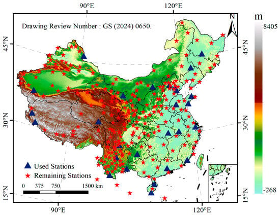
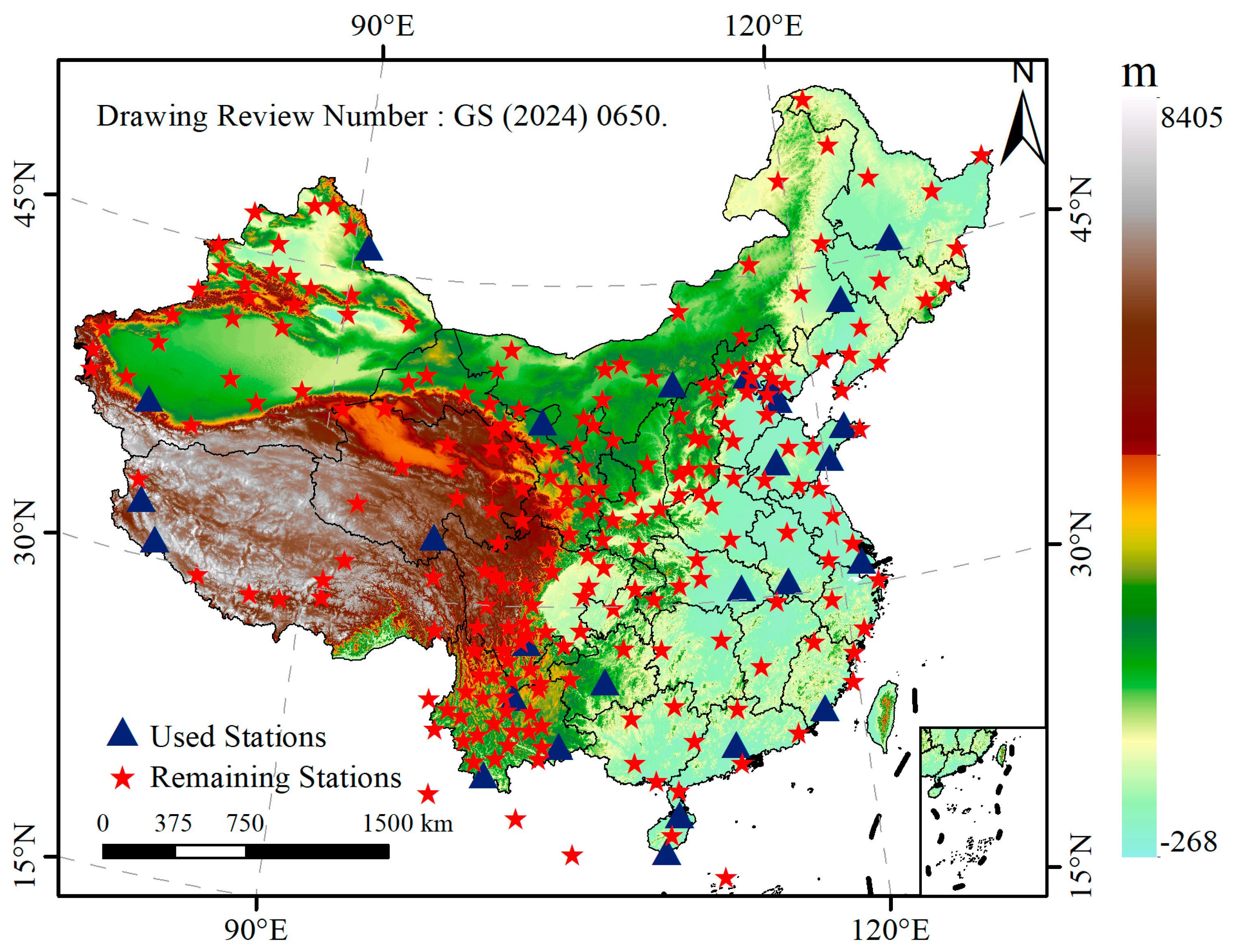
The China Crustal Movement Observation Network (CMONOC) is a national scientific infrastructure designed for monitoring crustal deformation across mainland China [17,18,19]. Initiated in 1997 and fully operational since 2011, CMONOC plays a vital role in detecting crustal movements, variations in the Earth’s gravity field, fluctuations in tropospheric water vapor, and ionospheric electron concentrations. These observations provide high-precision datasets that support research on the spatiotemporal characteristics of crustal dynamics and GNSS meteorology [20]. The network comprises more than 260 continuously operating reference stations and approximately 2000 non-continuous observation stations [21]. In this study, 27 continuously operating GNSS stations were selected from CMONOC to evaluate the proposed ZTD prediction model under different geographical and climatic conditions. Figure 1 shows the spatial distribution of the selected stations across China. Detailed station information, including geographic unit, station code, longitude, latitude, normal height, and climate type, is summarized in Table 1. According to their geographical and climatic characteristics, the selected stations were grouped into five regional climate categories: subtropical monsoon (SM), tropical monsoon (TRM), temperate monsoon (TEM), temperate continental (TEC), and plateau mountain (PM).

Figure 1. Distribution of CMONOC stations in China. The blue triangles represent Used stations; the red pentagram represent Remaining stations.

Table 1. Description of the GNSS station network used in this study.

Geographic Unit	Site Code	Longitude (°E)	Latitude (°N)	Normal Height (m)	Climate Type
Eastern Coastal Area	GUAN	113.34	23.18	30.93	SM
	HIHK	110.25	19.99	55.22	TRM
	HISY	109.53	18.24	47.00	TRM
	SDQD	120.30	36.08	11.71	TRM
	SDYT	121.44	37.48	92.41	TRM
	SHAO	121.20	31.10	21.77	SM
	XIAM	118.08	24.45	104.19	SM
Northeast Plain	HRBN	126.62	45.70	198.24	TEM
	NMAG	122.63	43.30	214.80	TEM
North China Transition Zone	BJYQ	115.97	40.37	584.71	TEM
	TAIN	117.12	36.21	338.87	TEM
	TJBH	117.69	39.08	−0.82	TEM
	TJBD	117.40	39.70	−0.50	TEM
Central China Hub	AHAQ	116.99	30.62	57.78	SM
	WUHN	114.36	30.53	25.81	SM
Southwest Complex Terrain	GZGY	106.67	26.47	1093.97	SM
	SCXD	102.44	28.30	1825.86	SM
	YNMH	100.45	21.95	1166.25	SM
	YNWS	104.25	23.41	1451.58	SM
	YNYM	101.86	25.69	1077.80	PM
Northwest Arid Region	GSMQ	103.09	38.63	1320.07	TEC
	NMTK	111.25	40.26	1004.03	TEC
	XJHT	79.05	37.16	1571.76	TEC
	XJQH	90.98	46.15	1105.41	TEC
Qinghai–Tibet Plateau	QHYS	97.01	33.01	3704.38	PM
	XZBG	81.43	30.84	4705.03	PM
	XZGE	80.11	32.52	4427.37	PM

2.2. ERA5 Data

The ERA5 reanalysis data, released by the European Centre for Medium-Range Weather Forecasts (ECMWF), represent the fifth-generation global atmospheric reanalysis product and serve as a successor to ERA-Interim [22]. ERA5 employs an advanced data assimilation system that integrates multiple sources of meteorological observations to provide a more accurate representation of the atmospheric state. Compared with its predecessor, ERA5 offers significantly improved spatial and temporal resolutions, with the temporal resolution increased from 6 h to 1 h, the horizontal grid resolution refined from approximately 79 km to 31 km, and the vertical resolution enhanced from 60 to 137 pressure levels, extending up to 0.01 hPa.

3. Methodology

3.1. ICEEMDAN Method

Empirical mode decomposition (EMD) was first proposed by Huang et al. [23]. It is a multi-scale decomposition method suitable for nonlinear, non-stationary and complex time series data. To address the modal aliasing problem of EMD, Wu and Huang have proposed ensemble empirical mode decomposition (EEMD) [24], complementary ensemble empirical mode decomposition (CEEMD) [25], and complete ensemble empirical mode decomposition with adaptive noise (CEEMDAN) [26]. Despite these improvements, CEEMDAN still suffers from residual noise and spurious modes. To overcome these limitations, Colominas et al. introduced ICEEMDAN in 2014 [27]. As an optimized version of CEEMDAN, ICEEMDAN suppresses modal aliasing by repeatedly introducing adaptive noise and performing ensemble averaging, thereby significantly improving signal decomposition accuracy.

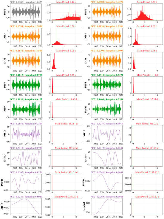
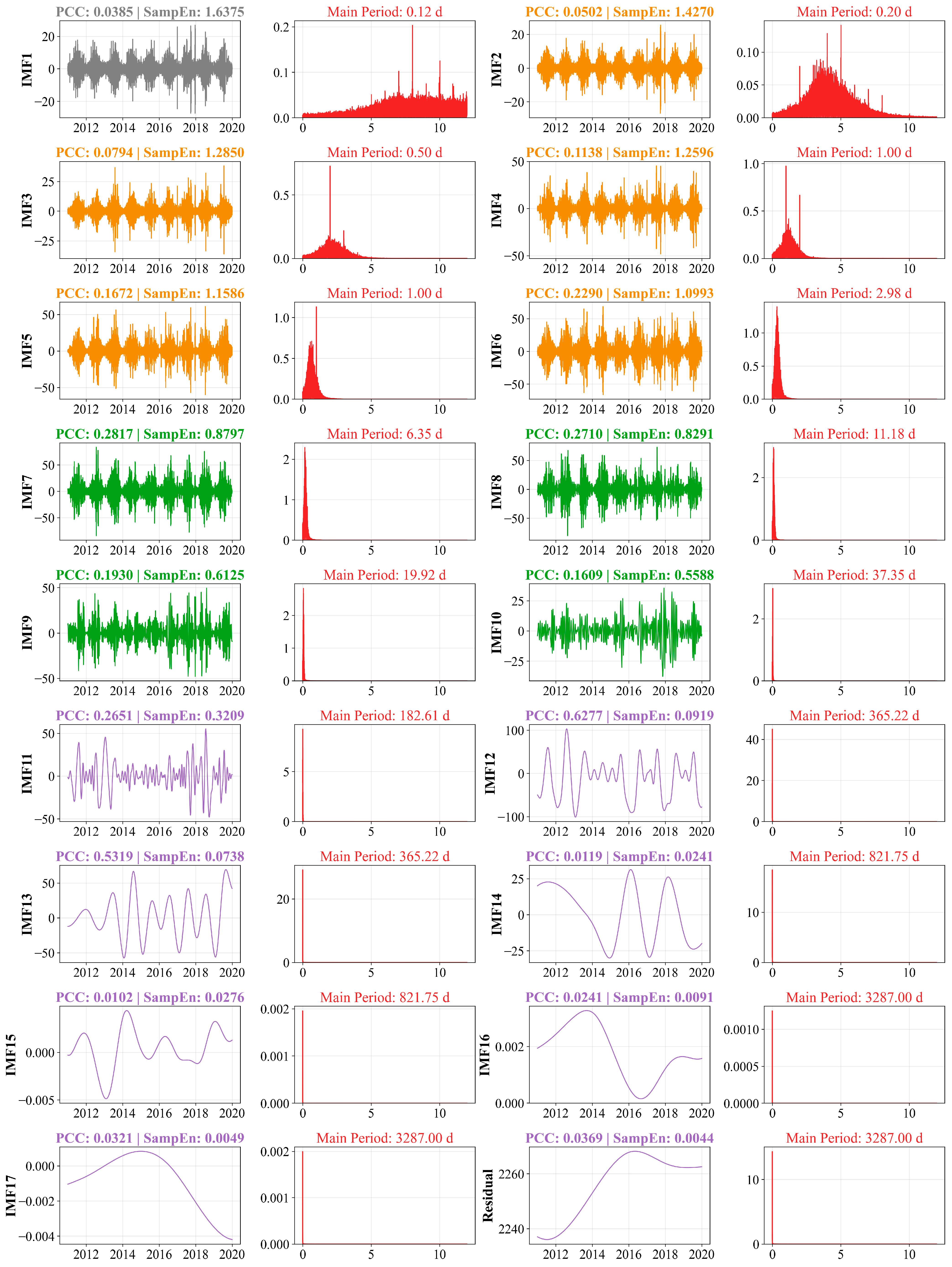
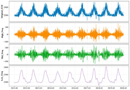
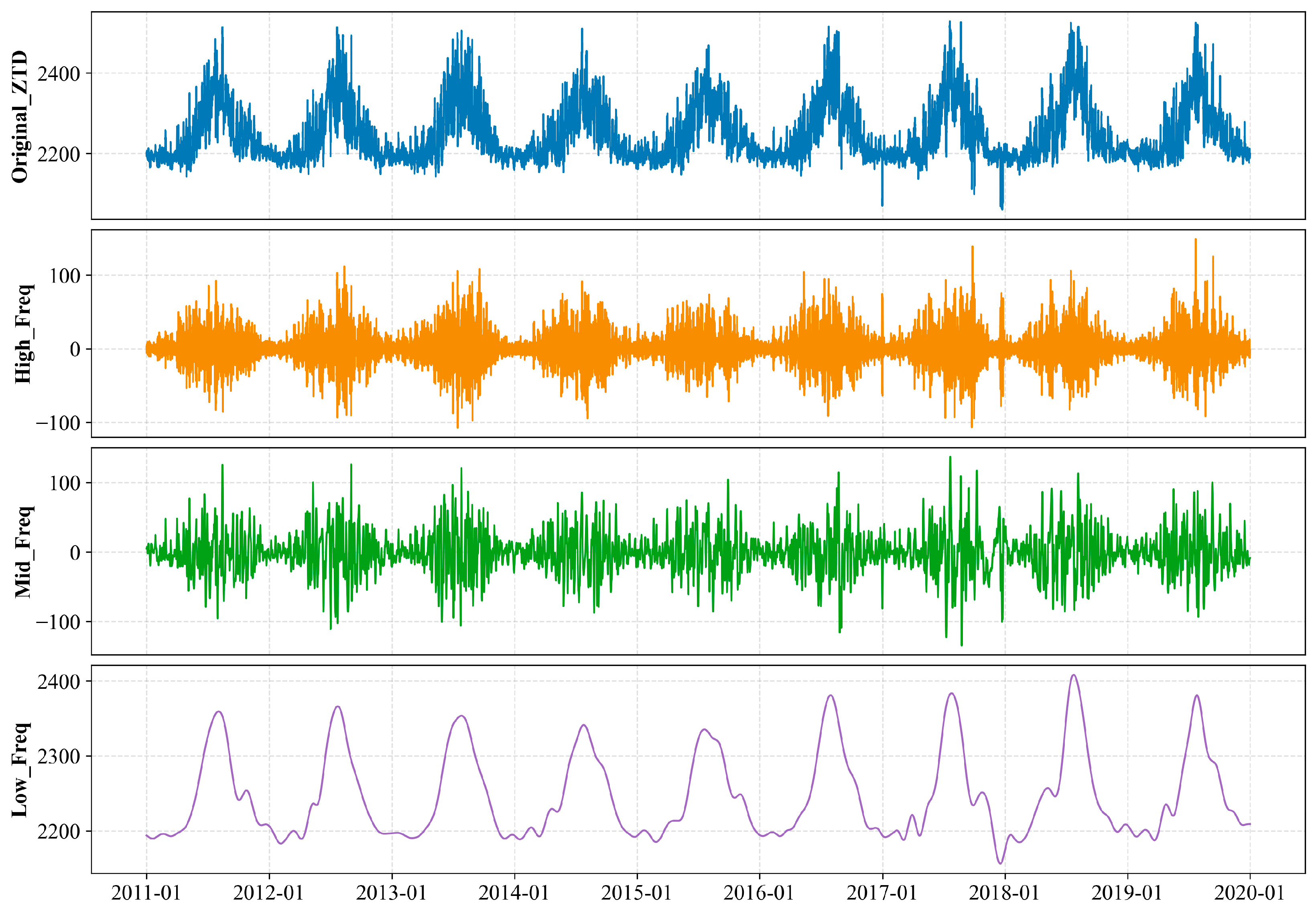
To ensure the reproducibility of the decomposition and reconstruction process, this study defines an explicit three-criterion intrinsic mode function (IMF) reconstruction strategy based on the dominant period, Pearson correlation coefficient (PCC), and sample entropy (SampEn). These criteria were used to characterize the temporal scale, consistency with the original ZTD series, and complexity of each IMF, respectively. The thresholds were determined by considering the statistical distribution of the decomposed IMFs, the physical variability of ZTD, and the performance on the validation set. Specifically, IMFs with a dominant period longer than 150 days were first assigned to the low-frequency component, as they mainly represent slowly varying seasonal signals. For the remaining IMFs, the absolute PCC between each IMF and the original ZTD series was calculated. Components with |PCC| < 0.05 were treated as noise-dominated or weakly related components and were removed from the reconstruction. The remaining IMFs were then further classified using SampEn = 1.0 as the complexity threshold. Components with SampEn > 1.0 were assigned to the high-frequency component, which mainly reflects short-term local variability such as convective disturbances and frontal passages. Components with SampEn ≤ 1.0 were assigned to the medium-frequency component, which captures relatively smoother intraseasonal oscillations driven by large-scale circulation. The ICEEMDAN decomposition result is shown in Figure 2. The reconstructed high-, medium-, and low-frequency subsequences are presented in Figure 3.

Figure 2. Decomposition results of ICEEMDAN.

Figure 3. Reconstructed ZTD subsequences based on the proposed three-criterion strategy.

3.2. BiLSTM Model

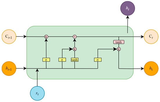
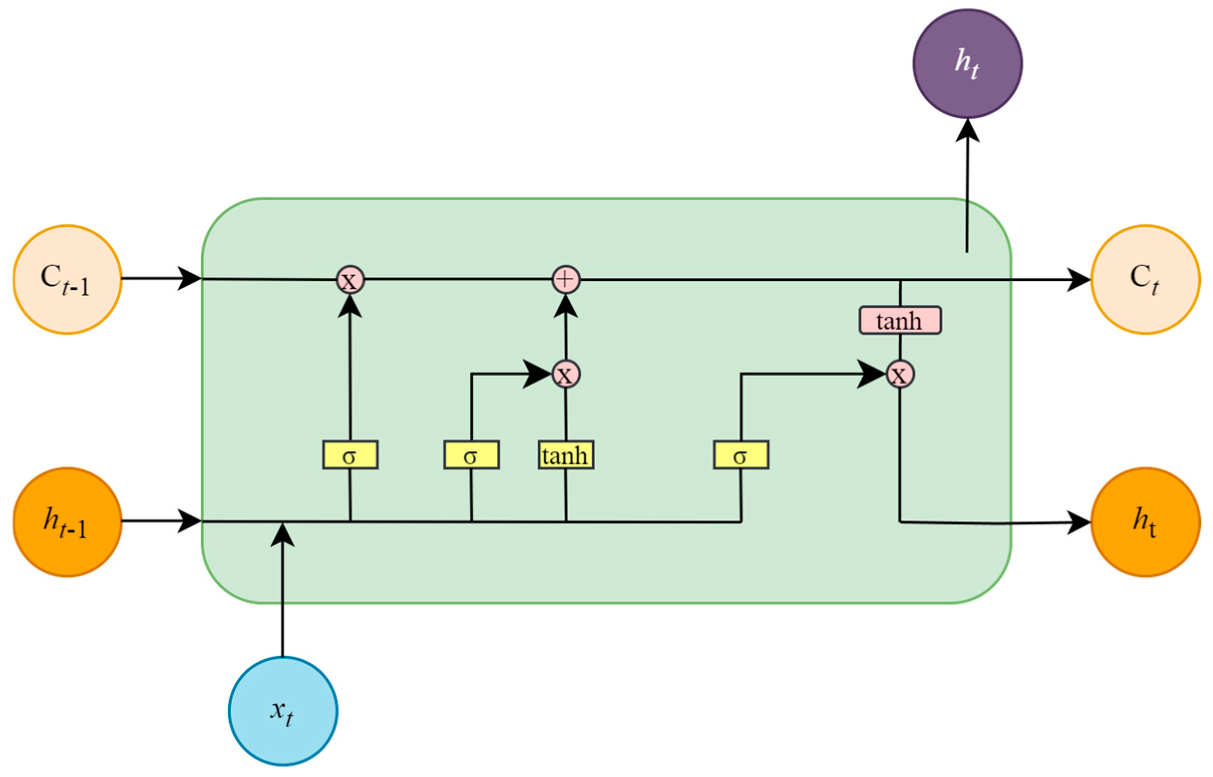
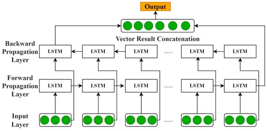
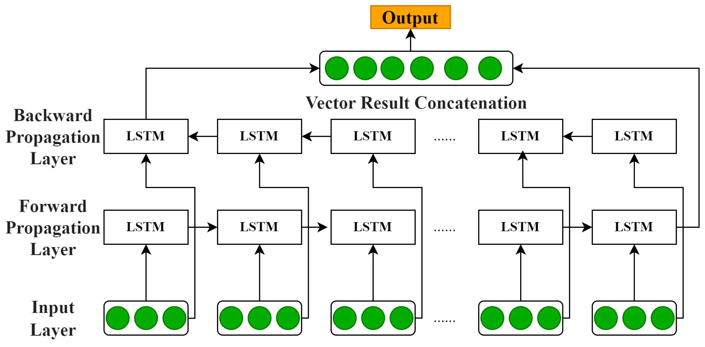
BiLSTM, an advanced extension of the standard long short-term memory (LSTM) architecture, is developed to address the inherent limitations of unidirectional sequence modeling [28]. In conventional LSTMs, information flow is regulated by three gating mechanisms—the input gate, forget gate, and output gate—which dynamically filter, store, and transmit temporal information through the cell state [29]. This gating structure not only enables efficient long-term dependency modeling but also effectively mitigates the vanishing gradient problem commonly encountered in recurrent neural networks (RNNs). The structure of a single LSTM cell is illustrated in Figure 4. However, a limitation of the standard unidirectional LSTM is that it can only propagate information forward based on historical data, which leaves a modeling blind spot in tasks requiring the incorporation of future context [30]. To overcome this drawback, the BiLSTM introduces a bidirectional interaction mechanism by combining a forward LSTM (→) and a backward LSTM (←). The forward layer extracts feature from past information, while the backward layer captures dependencies from future sequences [31]. By concatenating the hidden states from both directions, the BiLSTM achieves deep integration of contextual information.

Figure 4. LSTM cell structure diagram.

Mathematically, given an input sequence {x₁, x₂, …, x_t}, the BiLSTM generates two hidden states (h_t) at each time step t, these are then concatenated to produce the final representation:

$${\widehat{h}}_t=LST{M}_{\mathrm{fwd}}\left(x_t\right),{\widehat{h}}_t=LST{M}_{\mathrm{bwd}}\left(x_t\right)$$

(1)

$$h_t=[{\overrightarrow{h}}_t;{\tilde{h}}_t]$$

(2)

Figure 5 illustrates the architecture of the model. This design not only preserves the long-term dependency modeling capability of the LSTM but also enables the model to make decisions with access to both historical and future information. Such bidirectional coordination significantly improves the completeness of sequence modeling and enhances prediction accuracy.

Figure 5. BiLSTM model flow chart. The green circles denote the input feature vectors at the input layer and the output feature vectors after vector result concatenation.

3.3. XGBoost Model

XGBoost is a classical Boosting-based ensemble method, where the weak learner is a classification and regression tree (CART). As an optimized implementation of gradient boosting, XGBoost iteratively enhances model accuracy by fitting the negative gradient of the loss function [32,33]. At each iteration, the gradient between the current prediction and the true target is computed and used as the new training signal for a CART model. The outputs of all trees are then aggregated to form a strong learner, endowing XGBoost with exceptional predictive capability [34]. The algorithmic workflow of XGBoost is illustrated in Figure 6.

Figure 6. Schematic diagram of XGBoost principle.

The loss function in XGBoost measures the discrepancy between the predicted value $y_i$ and the actual value ${\widehat{y}}_i$. Here, k denotes the number of trees in the ensemble, and $\mathsf{\Omega }(f_k)$ represents the regularization term of the k-th tree, which is introduced to prevent overfitting. The loss function is defined as:

$$\mathrm{L}(\theta )={\displaystyle \sum _{i=1}^{n}l}\left({\widehat{y}}_i,y_i\right)+{\displaystyle \sum _{k=1}^K\mathsf{\Omega }}\left(f_k\right)$$

(3)

where l(.) is a differentiable convex loss function that measures the difference between the predicted value and the actual value. The regularization term of the k-th regression tree is given by:

$$\mathsf{\Omega }(f_k)=\gamma T+{\displaystyle \frac{1}{2}}\lambda \underset{j=1}{\sum ^T}{w}_j^2$$

(4)

where T is the number of leaf nodes, $w_j$ is the prediction score on the j-th leaf node, and γ and λ are regularization parameters that control model complexity.

3.4. IBX Model

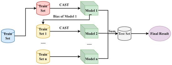
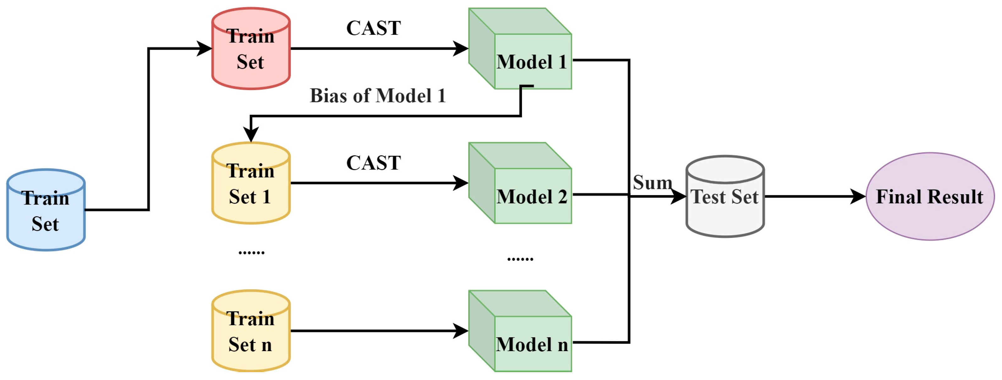
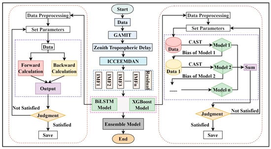
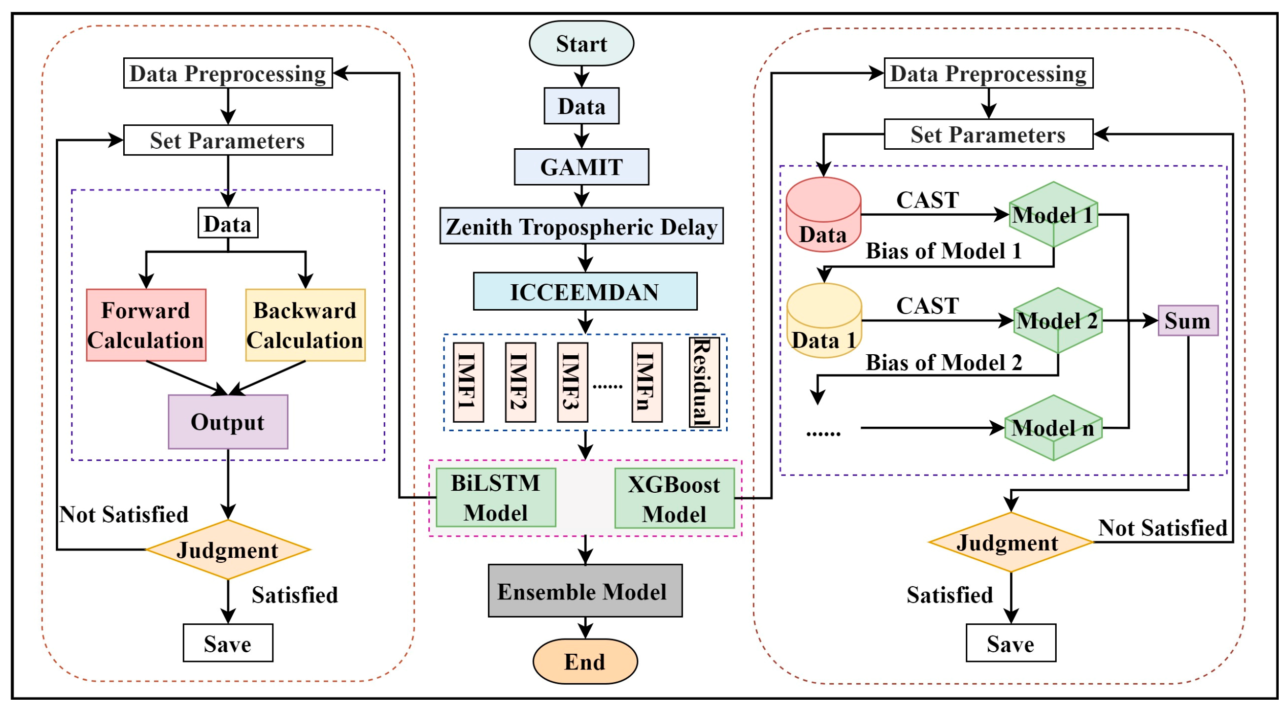
The overall workflow of the proposed IBX model is shown in Figure 7. The proposed IBX model consists of three main stages: ICEEMDAN-based decomposition, component-wise prediction, and adaptive fusion.

Figure 7. IBX model flow chart.

First, the original ZTD series is decomposed into high-, medium-, and low-frequency components using the reconstruction strategy described in Section 3.1. These components represent ZTD variations at different temporal scales and provide physically interpretable inputs for subsequent prediction. To evaluate the forecasting performance at different horizons, a multi-step rolling prediction strategy is adopted. The model uses ZTD observations from the previous 12 h as input and progressively predicts ZTD values from 1 to 12 h ahead. The 12 h input window was selected to capture recent sub-daily ZTD variability while limiting the input dimension for real-time rolling prediction. At each forecasting step, the prediction from the previous step is fed back into the input window to form an autoregressive forecasting chain. For the ICEEMDAN-BiLSTM (IB) and ICEEMDAN-XGBoost (IX) models, the high-, medium-, and low-frequency components are predicted separately. At step t, the predicted value of each component is calculated as follows:

$${\widehat{C}}_i^{(t)}=f_{\mathrm{model}}(C_i^{(t-12)},C_i^{(t-11)},\dots ,C_i^{(t-1)})$$

(5)

$C_i^{\left(t\right)}$ denotes the predicted value of the $i$-th component at step $t$, and $f_{model}(\cdot )$ denotes the BiLSTM or XGBoost prediction function. The predicted values of all components are summed up to reconstruct the complete ZTD prediction.

$${\widehat{Z}}_{\mathrm{IB}/\mathrm{IX}}^{(t)}={\displaystyle \sum _i{\widehat{C}}_i^{(t)}}$$

(6)

To combine the temporal modeling capability of BiLSTM with the nonlinear fitting capability of XGBoost, an RMS-based weighted fusion strategy is further introduced. The fusion weights are calculated according to the validation-set performance of the IB and IX models. A model with a lower validation RMS is assigned a higher weight:

$$w_{\mathrm{IB}}={\displaystyle \frac{1/{\mathrm{RMSE}}_{\mathrm{IB}}}{1/{\mathrm{RMSE}}_{\mathrm{IB}}+1/{\mathrm{RMSE}}_{\mathrm{IX}}}},\hspace{1em}\hspace{1em}{w}_{\mathrm{IX}}={\displaystyle \frac{1/{\mathrm{RMSE}}_{\mathrm{IX}}}{1/{\mathrm{RMSE}}_{\mathrm{IB}}+1/{\mathrm{RMSE}}_{\mathrm{IX}}}}$$

(7)

The final prediction of the IBX model is obtained as follows:

$${\widehat{Z}}_{\mathrm{IBX}}^{(t)}=w_{\mathrm{IB}}\cdot {\widehat{Z}}_{\mathrm{IB}}^{(t)}+w_{\mathrm{IX}}\cdot {\widehat{Z}}_{\mathrm{IX}}^{(t)}$$

(8)

This fusion strategy allows IBX to retain the short-term temporal sensitivity of BiLSTM while benefiting from the relatively stable nonlinear fitting ability of XGBoost. Therefore, the proposed model can reduce the error propagation risk in multi-step rolling prediction and improve the robustness of ZTD forecasting.

4. Results and Analysis

4.1. Experimental Settings and Evaluation Metrics

In this study, hourly ZTD series from 27 continuously operating GNSS stations in China were used as experimental samples. The station observations were processed using GAMIT 10.71 to derive ZTD values, which were then used as target values for prediction experiments. The ZTD series were sampled at 1 h intervals. To ensure chronological consistency and avoid information leakage, the dataset was divided into training, validation, and test sets according to the temporal order, with proportions of 70%, 15%, and 15%, respectively. Before model training, ERA5 reanalysis data were used as auxiliary reference data to identify and interpolate potential missing values in the training set. This preprocessing step ensured a sufficient number of valid samples and reduced the risk of fitting errors caused by data sparsity. The validation set was used for hyperparameter selection and fusion-weight determination, while the test set was used only for final model evaluation.

Five ZTD prediction models were constructed for comparison: XGBoost (X), BiLSTM (B), ICEEMDAN-XGBoost (IX), ICEEMDAN-BiLSTM (IB), and ICEEMDAN-BiLSTM-XGBoost (IBX). For the X and B models, the input features consisted of the original ZTD series with lagged values from 1 to 12 h. For the IX and IB models, ICEEMDAN decomposition was applied to the lagged ZTD components, and the reconstructed high-, medium-, and low-frequency components were used as input features. The IBX model further fused the predictions of IB and IX using RMS based weighting strategy described in Section 3.4. The hyperparameters of BiLSTM and XGBoost were optimized using a grid search strategy. For each candidate parameter combination, the model was trained on the training set and evaluated on the independent validation set. The parameter combination with the lowest validation RMS was selected as the optimal configuration and was then applied to the test set. For ICEEMDAN, the ensemble size was set to 20, the noise standard deviation to 0.1, the maximum number of IMFs to 20, and the maximum number of iterations to 100. For BiLSTM, the number of hidden units was selected from {32, 64}, the number of network layers from {1, 2}, the learning rate from {0.001, 0.005}, the training epochs from {50, 100}, and the batch size from {16, 32}. For XGBoost, the number of trees was set to 500, the learning rate was selected from {0.05, 0.1, 0.2}, the maximum depth from {3, 5, 10}, and the early stopping rounds to 20.

To evaluate model performance, the mean absolute error (MAE), root mean square error (RMS), and correlation coefficient (R) were used as accuracy metrics [35,36,37]. MAE reflects the average magnitude of prediction errors, RMS gives greater weight to large errors, and R measures the temporal consistency between predicted and reference ZTD values. Their expressions are given as follows:

$$\mathrm{MAE}={\displaystyle \frac{1}{n}}{\displaystyle \sum _{i=1}^n}|{\widehat{x}}_i-x_i|$$

(9)

$$\mathrm{RMS}=\sqrt{{\displaystyle \frac{1}{n}}{\displaystyle \sum _{i=1}^n{({\widehat{x}}_i-x_i)}^2}}$$

(10)

$$R={\displaystyle \frac{{\displaystyle \sum _{i=1}^n({\widehat{x}}_i-\overline{\widehat{x}})}(x_i-\overline{x})}{\sqrt{{\displaystyle \sum _{i=1}^n{({\widehat{x}}_i-\overline{\widehat{x}})}^2}}\sqrt{{\displaystyle \sum _{i=1}^n{(x_i-\overline{x})}^2}}}}$$

(11)

where n is the number of samples, x_i is the reference ZTD value, x-hat_i is the predicted ZTD value, x-bar is the mean reference value, and x-hat-bar is the mean predicted value.

4.2. Multi-Step Forecasting Performance

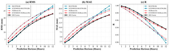
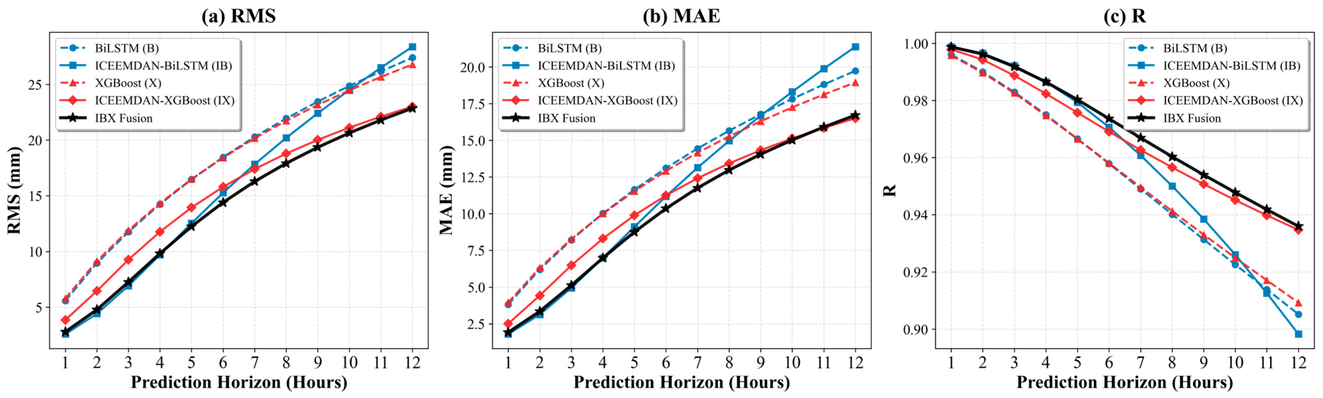
As shown in Figure 8, the RMS and MAE of all models generally increase as the forecasting horizon extends, while the correlation coefficient R decreases. This indicates that prediction uncertainty accumulates during multi-step rolling forecasting. Among the five models, IBX achieves the best overall performance across most forecasting horizons. In the short-term range of 1–5 h, IB performs close to IBX and clearly outperforms the baseline X and B models. This suggests that ICEEMDAN decomposition effectively improves short-term ZTD prediction by separating components at different temporal scales. However, the advantage of IB decreases as the forecasting horizon increases. From the 6 h horizon onward, the RMS and MAE of IB increase more rapidly. At the 12 h horizon, its RMS becomes higher than that of the original BiLSTM model. In contrast, IBX maintains a more stable error growth pattern. At the 12 h horizon, its RMS is limited to approximately 22.86 mm, with R remaining above 0.87. These results show that IBX provides the most robust multi-step forecasting performance among the tested models.

Figure 8. Performance Evaluation of Different Models Across Various Prediction Horizons.

4.3. Altitude-Based Validation

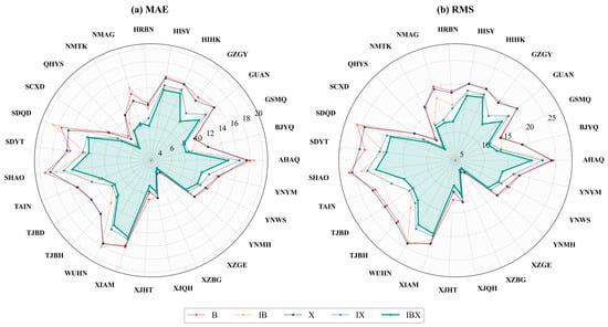
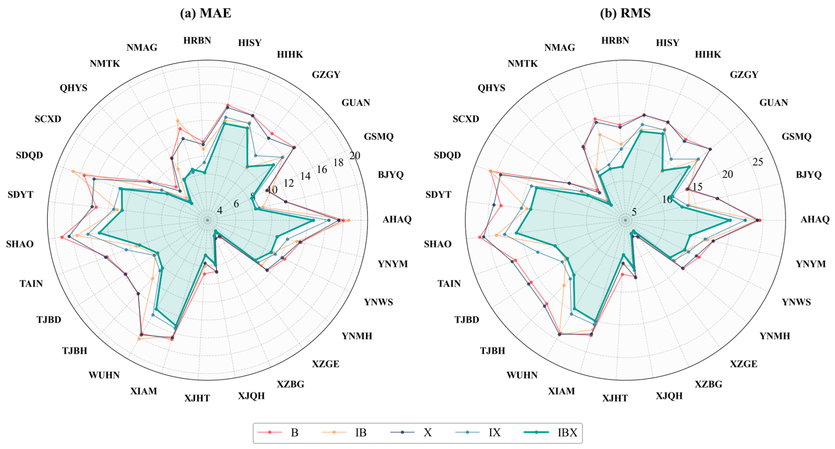
Figure 9 shows the station-wise average forecasting errors of the five models across the 27 GNSS stations using radar charts, including MAE and RMS. Since a smaller radial distance indicates a lower prediction error, the radar profiles provide a direct comparison of model performance at different stations. The pronounced variations in the profiles reveal the spatial heterogeneity of ZTD prediction accuracy, which is jointly affected by station altitude, geographical location, and regional moisture conditions. Previous analyses of GNSS-derived precipitable water vapor (PWV) over China have shown that atmospheric water vapor exhibits significant spatial differences among climate regions, with higher PWV values and larger annual amplitudes in tropical and subtropical monsoon regions than in plateau and continental regions [38]. In addition, ZTD modeling over regions with large elevation differences is strongly affected by vertical variation, indicating that altitude is an important factor controlling tropospheric delay estimation [18]. Overall, stations located in eastern coastal and low-altitude regions, such as HIHK, SHAO, and SDYT, with elevations below 200 m, show relatively large errors. Their MAE values are generally between 14 and 20 mm, while their RMS values exceed 20 mm. These stations form clear outward protrusions in the radar profiles. This pattern is likely related to the strong variability of water vapor fields in coastal and monsoon-affected regions, which increases the difficulty of nonlinear ZTD prediction. In contrast, high-altitude stations on the Qinghai–Tibet Plateau, such as XZGE and XZBG, with elevations above 4000 m, show a clear inward contraction in the radar profiles. Their MAE values decrease to approximately 4–8 mm. This result is consistent with previous findings that PWV is negatively correlated with altitude and that plateau regions generally have lower atmospheric water vapor content [38]. The reduced atmospheric column and lower water vapor content at high altitudes weaken ZTD variability and improve prediction stability. When the five models are compared, the shaded area enclosed by the IBX fusion model is generally located closest to the center across most stations, indicating lower prediction errors. This advantage is particularly evident at high-error stations such as SDYT and SHAO, where IBX shows a stronger inward contraction than the baseline models. These results indicate that the ICEEMDAN-based decomposition and dynamic fusion strategy improves the robustness and spatial adaptability of ZTD prediction under complex water vapor conditions.

Figure 9. Radar chart representations of (a) MAE and (b) RMS errors for X, IX, B, IB, and IBX, evaluated on the test set.

4.4. Climate-Type Validation

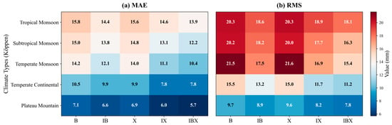
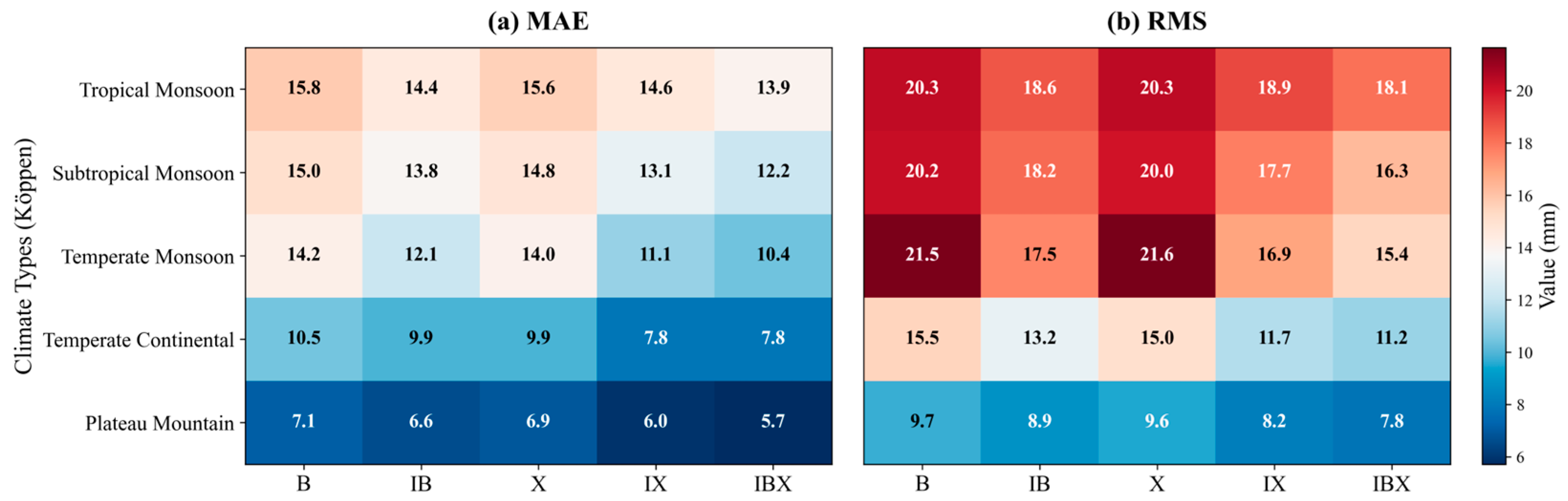
Figure 10 presents the average MAE and RMS of the five models across different regional climate categories. The results show a clear gradient in prediction accuracy among climate regions. In water-vapor-rich tropical and subtropical monsoon regions, all models show relatively high errors, with RMS values above 16 mm. In contrast, in the dry plateau mountain region, the IBX model achieves an MAE of only 5.7 mm and an RMS of 7.8 mm. This pattern is consistent with previous GNSS-PWV studies over China, which reported that PWV is significantly higher in tropical and subtropical monsoon regions than in plateau and continental regions, and that PWV is negatively correlated with altitude [38]. These results support the view that the spatiotemporal variability of atmospheric water vapor is an important physical factor limiting ZTD prediction accuracy.

Figure 10. Comparison of MAE (a) and RMS (b) Errors of Five ZTD Prediction Models across regional climate categories in China.

Notably, the IBX model shows the most pronounced improvement in the temperate monsoon region. Its RMS decreases from 21.5 mm for the baseline B model to 15.4 mm, corresponding to an improvement rate of 28.4%. This improvement may be related to the strong seasonal variability of ZTD in the temperate monsoon region, where the contrast between winter and summer atmospheric conditions is relatively clear. ICEEMDAN decomposition helps separate seasonal and short-term components of the ZTD series. When combined with the BiLSTM-XGBoost hybrid architecture, this decomposition allows IBX to better handle high-variability signals. This may explain why the improvement of IBX is more evident in the temperate monsoon region than in regions dominated by stronger random water vapor disturbances. Overall, the IBX model achieves the lowest errors in all five climate categories. This indicates that the proposed fusion model has good adaptability and generalization ability under different climatic backgrounds.

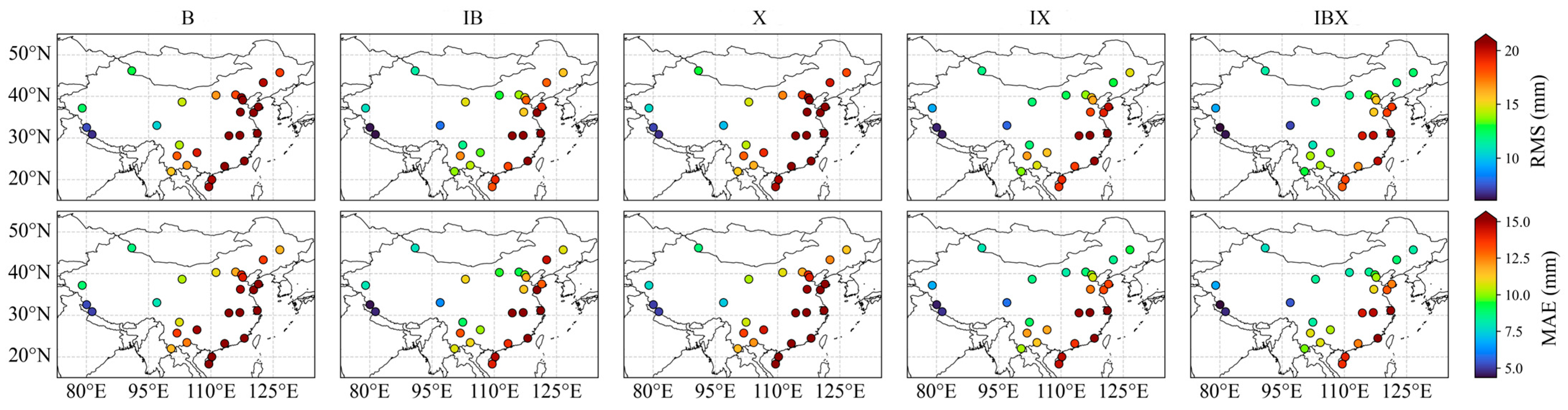
4.5. Geographic Coverage Validation

Figure 11 and Table 2 evaluate the overall forecasting performance of the five models from two perspectives: geospatial distribution and multi-station statistics. The spatial distribution maps show clear regional differences in ZTD prediction accuracy. Relatively large errors are observed at southeastern coastal stations, such as HIHK and HISY, where the points are shown in warmer colors. In contrast, stations on the Qinghai–Tibet Plateau, such as XZGE and XZBG, generally show lower errors and are represented by cooler colors. This spatial pattern is consistent with the altitude- and climate-related characteristics discussed in Section 4.3 and Section 4.4.

Figure 11. Distribution of ZTD prediction accuracy on the test set across 27 stations in China.

Table 2. Average Precision over the 12 steps.

	RMS/mm			MAE/mm
Model	Max	Min	Mean	Max	Min	Mean
X	25.82	6.7	18.17	18.43	5.05	12.75
IX	22.61	6.38	15.29	16.41	4.62	10.88
B	26.43	6.74	18.29	19.25	5.09	13.02
IB	25.89	6.22	15.93	18.84	4.47	11.79
IBX	20.79	6.06	14.17	15.16	4.34	10.24

Compared with the other models, IBX shows a more consistent reduction in prediction errors across the station network. This improvement is particularly evident in central China, eastern China, and the arid regions of northwest China, where the colors of the IBX results become visibly lighter than those of the baseline models. These results indicate that the proposed fusion model is effective not only at individual stations, but also across broader geographical units with different terrain and moisture conditions. The statistical results in Table 2 further confirm the overall advantage of IBX over the 1–12 h forecasting horizons. IBX achieves the lowest mean RMS and MAE, with values of 14.17 mm and 10.24 mm, respectively. Compared with the baseline BiLSTM model, these values are reduced by 22.5% and 21.4%, respectively. In addition, IBX significantly lowers the upper bound of forecasting error. Its maximum RMS is 20.79 mm, which is lower than those of B and IX, with values of 26.43 mm and 22.61 mm, respectively. The combination of a low mean error and a reduced maximum error indicates that IBX has strong forecasting robustness and spatial generalization ability across different geographical environments. This suggests that the ICEEMDAN-based decomposition and BiLSTM-XGBoost fusion strategy can improve ZTD prediction stability over a heterogeneous station network.

5. Discussion

It can be observed from the multi-step prediction experiments that error accumulation is one of the main factors affecting ZTD forecasting accuracy. As the forecasting horizon increases, the proportion of predicted values in the input window gradually rises, which reduces the quality of the input information and leads to the continuous increase in RMS and MAE and the decrease in R. The IB model shows good performance in the short-term range, indicating that ICEEMDAN decomposition is useful for separating ZTD variations at different temporal scales. However, its advantage becomes weaker at longer horizons, which may be related to the recurrent structure of BiLSTM, where early prediction errors are repeatedly introduced into later inputs. By combining BiLSTM and XGBoost, the proposed IBX model reduces the dependence on a single recurrent predictor. The RMS-based weighted fusion strategy makes use of both temporal modeling and nonlinear fitting abilities, and therefore helps suppress the rapid growth of prediction errors in medium- and long-term forecasting. The spatial validation results show that the prediction accuracy is also related to station environment. Larger errors mainly occur at coastal and low-altitude stations, while high-altitude plateau stations generally show lower errors. This result is consistent with the physical characteristics of tropospheric delay. Coastal and monsoon-affected regions usually have more abundant and variable water vapor, which increases the uncertainty of ZTD prediction. In contrast, plateau stations have a shorter atmospheric column and lower water vapor content, resulting in weaker ZTD variability and better prediction stability. The climate-region-based results further show that errors are relatively high in tropical and subtropical monsoon regions, whereas the plateau mountain region has the lowest errors. The better performance of IBX in the temperate monsoon region may be related to the clearer seasonal variation in ZTD, which can be separated by ICEEMDAN and further modeled by the BiLSTM-XGBoost fusion framework.

Although IBX shows better performance than the tested models, a direct BiLSTM-XGBoost ensemble without ICEEMDAN decomposition was not included in this study. Therefore, the improvement of IBX should be regarded as the combined effect of component decomposition and hybrid prediction. Unlike numerical-weather-model-based mapping functions such as the Vienna Mapping Function, the current IBX framework does not directly use forecast meteorological fields as model inputs. The current model mainly relies on single-station historical ZTD series and does not explicitly include external meteorological drivers such as temperature, pressure, humidity, wind, and water vapor transport. This may limit its performance under long forecasting horizons and complex weather conditions. Future studies should include multi-source meteorological information and physical constraints, such as Saastamoinen-type tropospheric delay models, to further improve the robustness of ZTD prediction.

6. Conclusions

A multi-step rolling prediction model for ZTD, named IBX, was developed by combining ICEEMDAN-based component decomposition with a BiLSTM-XGBoost fusion architecture. The ICEEMDAN reconstruction strategy separates ZTD variations at different temporal scales and improves short-term prediction accuracy by reducing the interference of mixed-frequency components. However, the ICEEMDAN-BiLSTM model is still affected by error propagation during long-horizon rolling prediction. After introducing XGBoost and the RMS-based weighted fusion strategy, the proposed IBX model reduces the rapid error growth at longer forecasting horizons. Over the 1–12 h forecasting horizons, IBX obtains the lowest mean RMS and MAE among all tested models, with values of 14.17 mm and 10.24 mm, respectively, which are 22.5% and 21.4% lower than those of the baseline BiLSTM model. The maximum RMS is also reduced to 20.79 mm, indicating that the proposed fusion strategy can reduce the upper range of prediction errors. The station-wise, altitude-related, and climate-region-based analyses show that ZTD prediction accuracy is affected by geographical and climatic conditions. Larger errors mainly occur in coastal and monsoon-affected low-altitude regions, while plateau stations show lower errors. IBX achieves the lowest errors across all five climate categories, suggesting that the proposed model has good adaptability under different station environments. Overall, the IBX model provides an effective approach for short- to medium-term ZTD forecasting and can support atmospheric delay correction in real-time precise positioning. Future work will focus on improving long-horizon prediction by introducing multi-source meteorological variables and physical constraint mechanisms.

References

- Huang, L.; Liu, L.; Yao, C. A Zenith Tropospheric Delay Correction Model Based on the Regional CORS Network. Geod. Geodyn. 2012, 3, 53–62. [Google Scholar] [CrossRef] [Scilit]
- Zhang, K.; Li, H.; Wang, X.; Zhu, D.; He, Q.; Li, L.; Hu, A.H.A.; Zheng, N.; Li, H. Recent Progresses and Future Prospectives of Ground-Based GNSS Water Vapor Sounding. Cehui Xuebao/Acta Geod. Cartogr. Sin. 2022, 51, 1172–1191. [Google Scholar] [CrossRef]
- Li, J.; Li, F.; Zhang, B.; Yao, Y.; Liu, L.; Huang, L.; Wang, X. Case Study on Zenith Hydrostatic Delay Calibration Models for Forecast Vienna Mapping Function 3 and Their Impact on GNSS Precipitable Water Vapor Retrieval. IEEE Trans. Geosci. Remote Sens. 2026, 64, 4102812. [Google Scholar] [CrossRef] [Scilit]
- Yao, Y.; Zhao, Q. Research Progress and Prospect of Monitoring Tropospheric Water Vapor by GNSS Technique. Acta Geod. Cartogr. Sin. 2022, 51, 935. [Google Scholar] [CrossRef]
- Zhao, Q.; Liu, K.; Sun, T.; Yao, Y.; Li, Z. A Novel Regional Drought Monitoring Method Using GNSS-Derived ZTD and Precipitation. Remote Sens. Environ. 2023, 297, 113778. [Google Scholar] [CrossRef] [Scilit]
- Li, J.; Zhang, Q.; Liu, L.; Yao, Y.; Huang, L.; Chen, F.; Zhou, L.; Zhang, B. A Refined Zenith Tropospheric Delay Model for Mainland China Based on the Global Pressure and Temperature 3 (GPT3) Model and Random Forest. GPS Solut. 2023, 27, 172–184. [Google Scholar] [CrossRef] [Scilit]
- Huang, L.; Bi, H.; Zhang, H.; Wang, S.; Liao, F.; Liu, L.; Jiang, W. An Optimized BP Neural Network for Modeling Zenith Tropospheric Delay in the Chinese Mainland Using Coupled Particle Swarm and Genetic Algorithm. Geo-Spat. Inf. Sci. 2024, 28, 1927–1942. [Google Scholar] [CrossRef] [Scilit]
- Huang, L.; Liu, L.; Wen, H. Single-Site Improvement and Accuracy Analysis for Zenith Tropospheric Delay of EGNOS Model over Asia Area. Acta Geod. Cartogr. Sin. 2014, 43, 808–817. [Google Scholar] [CrossRef]
- Chen, J.; Wang, J.; Wang, J.; Tan, W. SHAtrop: Empirical ZTD Model Based on CMONOC GNSS Network. Geomat. Inf. Sci. Wuhan Univ. 2019, 44, 1588–1595. [Google Scholar] [CrossRef]
- Li, J.; Li, F.; Liu, L.; Yao, Y.; Huang, L.; Wang, Y. A Weighted Mean Temperature Forecast Model Based on Fused Data and Generalized Regression Neural Network and Its Impact on GNSS-Based Precipitable Water Vapor Estimation. IEEE Trans. Geosci. Remote Sens. 2024, 62, 4101914. [Google Scholar] [CrossRef] [Scilit]
- Byun, S.H.; Bar-Sever, Y.E. A New Type of Troposphere Zenith Path Delay Product of the International GNSS Service. J. Geod. 2009, 83, 1–7. [Google Scholar] [CrossRef] [Scilit]
- Yang, J.; Gu, H.; Liu, Y.; Wu, L.; Gao, Y. Study on GPS Tropospheric Delay Variation Based on Wavelet Analysis. Bull. Surv. Mapp. 2015, 60–62. [Google Scholar] [CrossRef]
- Lv, H.; Huang, W.; Wen, D. A Tropospheric Delay Prediction Model Based on Spectrum Analysis and the AR Compensation. J. Geod. Geodyn. 2015, 35, 283–286. [Google Scholar] [CrossRef]
- Wang, X.; Zhang, Q.; Zhang, S. Periodic Oscillation Analysis of GPS Water Vapor Time Series Using Combined Algorithm Based on EMD and WD. Geomat. Inf. Sci. Wuhan Univ. 2018, 43, 621–628. [Google Scholar] [CrossRef]
- Zhang, X.; Dang, Y.; Xu, C. A New GPT2w Model Improved by PSO-LSSVM for GNSS High-Precision Positioning. J. Sens. 2021, 2021, 9990831. [Google Scholar] [CrossRef] [Scilit]
- Mirmohammadian, F.; Asgari, J.; Verhagen, S.; Amiri-Simkooei, A. Multi-GNSS-Weighted Interpolated Tropospheric Delay to Improve Long-Baseline RTK Positioning. Sensors 2022, 22, 5570. [Google Scholar] [CrossRef] [Scilit] [PubMed]
- Zhao, Q.; Yao, Y.; Yao, W.; Zhang, S. GNSS-Derived PWV and Comparison with Radiosonde and ECMWF ERA-Interim Data over Mainland China. J. Atmos. Sol. Terr. Phys. 2019, 182, 85–92. [Google Scholar] [CrossRef] [Scilit]
- Zhao, Q.; Wang, W.; Li, Z.; Du, Z.; Yang, P.; Yao, W.; Yao, Y. A High-Precision ZTD Interpolation Method Considering Large Area and Height Differences. GPS Solut. 2023, 28, 4. [Google Scholar] [CrossRef] [Scilit]
- Zhao, Q.; Zheng, D.; Yao, Y.; Yao, W. Combining Spatio-Temporal Weighting with Reanalysis Data for Filling in GNSS PWV Time Series. Acta Geod. Cartogr. Sin. 2023, 52, 1661–1668. [Google Scholar] [CrossRef]
- Zhao, Q.; Liu, K.; Li, Z.; Yao, W.; Yao, Y. PWV Inversion Method Based on GNSS and Non-Measured Meteorological Parameters and Accuracy Evaluation. Geomat. Inf. Sci. Wuhan Univ. 2024, 49, 453–464. [Google Scholar] [CrossRef]
- Liu, B.; Wang, Y.; Lou, Z.; Wei, Z. The MODIS PWV Correction Based on CMONOC in Chinese Mainland. Acta Geod. Cartogr. Sin. 2019, 48, 1207. [Google Scholar] [CrossRef]
- Hersbach, H.; Bell, B.; Berrisford, P.; Hirahara, S.; Horányi, A.; Muñoz-Sabater, J.; Nicolas, J.; Peubey, C.; Radu, R.; Schepers, D.; et al. The ERA5 Global Reanalysis. Q. J. R. Meteorol. Soc. 2020, 146, 1999–2049. [Google Scholar] [CrossRef] [Scilit]
- Huang, N.E.; Shen, Z.; Long, S.R.; Wu, M.C.; Shih, H.H.; Zheng, Q.; Yen, N.-C.; Tung, C.C.; Liu, H.H. The Empirical Mode Decomposition and the Hilbert Spectrum for Nonlinear and Non-Stationary Time Series Analysis. Proc. R. Soc. Lond. A Math. Phys. Eng. Sci. 1998, 454, 903–995. [Google Scholar] [CrossRef] [Scilit]
- Wu, Z.; Huang, N.E. Ensemble Empirical Mode Decomposition: A Noise-Assisted Data Analysis Method. Adv. Adapt. Data Anal. 2009, 1, 1–41. [Google Scholar] [CrossRef] [Scilit]
- Yeh, J.-R.; Shieh, J.-S.; Huang, N.E. Complementary Ensemble Empirical Mode Decomposition: A Novel Noise Enhanced Data Analysis Method. Adv. Adapt. Data Anal. 2010, 2, 135–156. [Google Scholar] [CrossRef] [Scilit]
- Shi, Y.; Yang, C.; Wang, J.; Zhang, Z.; Meng, F.; Bai, H. A Forecasting Model of Ionospheric foF2 Using the LSTM Network Based on ICEEMDAN Decomposition. IEEE Trans. Geosci. Remote Sens. 2023, 61, 4108416. [Google Scholar] [CrossRef] [Scilit]
- Colominas, M.A.; Schlotthauer, G.; Torres, M.E. Improved Complete Ensemble EMD: A Suitable Tool for Biomedical Signal Processing. Biomed. Signal Process. Control 2014, 14, 19–29. [Google Scholar] [CrossRef] [Scilit]
- Kamal Das, M.; Columbus Chinnappan, C.; Elakiya, E. A Temporal Attention-Based SARIMA-BiLSTM Residual Learning Model Tuned by Grey Wolf Optimizer for Parallel Urban Traffic Forecasting. IEEE Access 2025, 13, 136073–136086. [Google Scholar] [CrossRef] [Scilit]
- Luo, A.; Zhong, L.; Wang, J.; Wang, Y.; Li, S.; Tai, W. Short-Term Stock Correlation Forecasting Based on CNN-BiLSTM Enhanced by Attention Mechanism. IEEE Access 2024, 12, 29617–29632. [Google Scholar] [CrossRef] [Scilit]
- Ma, C.; Dai, G.; Zhou, J. Short-Term Traffic Flow Prediction for Urban Road Sections Based on Time Series Analysis and LSTM_BILSTM Method. IEEE Trans. Intell. Transp. Syst. 2022, 23, 5615–5624. [Google Scholar] [CrossRef] [Scilit]
- Xie, J.; Chen, B.; Gu, X.; Liang, F.; Xu, X. Self-Attention-Based BiLSTM Model for Short Text Fine-Grained Sentiment Classification. IEEE Access 2019, 7, 180558–180570. [Google Scholar] [CrossRef] [Scilit]
- Duan, S.; Lian, Y.; Zhao, E.; Chen, H.; Han, W.; Wu, Z. A Novel Approach to All-Weather LST Estimation Using XGBoost Model and Multisource Data. IEEE Trans. Geosci. Remote Sens. 2023, 61, 5004614. [Google Scholar] [CrossRef] [Scilit]
- Zhang, T.; Zhang, X.; Rubasinghe, O.; Liu, Y.; Chow, Y.H.; Iu, H.H.C.; Fernando, T. Long-Term Energy and Peak Power Demand Forecasting Based on Sequential-XGBoost. IEEE Trans. Power Syst. 2024, 39, 3088–3104. [Google Scholar] [CrossRef] [Scilit]
- Liu, B.; Guo, H.; Li, J.; Ke, X.; He, X. Application and Interpretability of Ensemble Learning for Landslide Susceptibility Mapping along the Three Gorges Reservoir Area, China. Nat. Hazard. 2024, 120, 4601–4632. [Google Scholar] [CrossRef] [Scilit]
- Zhao, Q.; Du, Z.; Wu, M.; Yao, Y.; Yao, W. Establishment of PWV Fusion Model Using Multi-Source Data. Geomat. Inf. Sci. Wuhan Univ. 2022, 47, 1823–1831. [Google Scholar] [CrossRef]
- Huang, L.; Lu, D.; Chen, F.; Zhang, H.; Zhu, G.; Liu, L. A Deep Learning-Based Approach for Directly Retrieving GNSS Precipitable Water Vapor and Its Application in Typhoon Monitoring. IEEE Trans. Geosci. Remote Sens. 2024, 62, 4111712. [Google Scholar] [CrossRef] [Scilit]
- Zhu, D.; Sun, P.; Hu, Q.; Zhang, K.; Wu, S.; He, P.; Yu, A.; Yin, W.; Liu, W.; Hu, Q. A Fusion Framework for Producing an Accurate PWV Map with Spatiotemporal Continuity Based on GNSS ERA5 and MODIS Data. IEEE Trans. Geosci. Remote Sens. 2024, 62, 5802214. [Google Scholar] [CrossRef] [Scilit]
- Yang, F.; Gong, X.; Li, Z.; Wang, Y.; Song, S.; Wang, H.; Chen, R. Spatiotemporal Distribution and Impact Factors of GNSS-PWV in China Based on Climate Region. Adv. Space Res. 2024, 73, 4187–4201. [Google Scholar] [CrossRef] [Scilit]
Disclaimer/Publisher’s Note: The statements, opinions and data contained in all publications are solely those of the individual author(s) and contributor(s) and not of MDPI and/or the editor(s). MDPI and/or the editor(s) disclaim responsibility for any injury to people or property resulting from any ideas, methods, instructions or products referred to in the content. |
© 2026 by the authors. Licensee MDPI, Basel, Switzerland. This article is an open access article distributed under the terms and conditions of the Creative Commons Attribution (CC BY) license.