


Highlights
What are the main findings?
- An 85.2% detection rate of real-world trees was achieved, with a 23.5% commission rate and a DBH RMSE of 1.98 cm (9.65%)
- Among evaluated stand-level variables, tree density (trees ha−1) and relative density showed a measurable, though minimal, influence on detection performance; other structural characteristics did not improve model fit.
What are the implications of the main findings?
- Results demonstrate that mobile LiDAR can produce highly accurate DBH estimates in complex, mixed-species forests, though detection performance, particularly commission error, remains a limiting factor for operational applications.
- The limited influence of stand-level characteristics suggests that detection performance is driven more strongly by tree-level attributes or unmeasured structural components such as understory complexity.
Abstract
Understanding forest dynamics requires reliable inventories that assess tree- and stand-level characteristics. Traditionally, this has relied on field measurements such as diameter at breast height (DBH), height, and crown attributes, but these methods are labor-intensive and spatially limited. Remote sensing, particularly Light Detection and Ranging (LiDAR), has expanded forest inventory capacity by generating three-dimensional structural information. Mobile laser scanning (MLS), a recent adaptation, offers flexible, high-resolution data collection, though its performance across complex forests is still being evaluated. This study assessed the effectiveness of MLS in detecting individual trees and estimating DBH in mixed-species forests of the Northeastern United States. We also evaluated the influence of tree- and plot-level characteristics on detection accuracy and DBH estimation. Results showed an 85.2% tree detection rate, a 23.5% commission rate, and a DBH root mean square error (RMSE) of 1.98 cm (9.65%). Among the variables tested, tree DBH was the only significant predictor of detection probability; tree density and relative density had minimal effect. These findings demonstrate that MLS can achieve precise DBH estimation when trees are correctly identified, but false detections remain a limitation. Further methodological improvements are needed to enhance accuracy in structurally complex forests and advance MLS for operational forest monitoring.
1. Introduction
Complex mixed-species forests have been found to support productive and resilient ecosystems while meeting important economic, social, and cultural objectives [1]. However, a key challenge in managing these systems lies in understanding the dynamics of species, including the interactions between structure, composition, and ecosystem function [2]. The emergence of precise and efficient forest measurement technologies, such as mobile Light Detection and Ranging (LiDAR), offers promising opportunities to improve understanding of these dynamic species interactions and support informed management of complex forest ecosystems [3].
LiDAR is an active remote sensing technology that emits laser pulses to measure distances based on the time it takes for the pulses to return from surfaces. Over the course of a scan, LiDAR sensors can collect hundreds of thousands of point returns, which are compiled into dense “point clouds” that digitally reconstruct the scanned environment in three dimensions. These point clouds can be processed to extract forest attributes and metrics such as individual tree locations, diameter at breast height (DBH), tree height, and crown structure—information that forms the foundation of species dynamics and functional interactions [2,4].
Traditionally, LiDAR has been deployed through aerial platforms, known as aerial laser scanning (ALS), using aircraft to enable large spatial scale forest mapping, and more recently through spaceborne platforms [5,6]. While high-resolution commercial and full-waveform ALS systems have demonstrated improved capabilities in capturing vertical forest structure, a common limitation of standard ALS datasets, particularly those with lower pulse density, is their reduced capacity to capture detailed information beneath dense forest canopies. This often results in incomplete or imprecise representations of understory structure or individual tree delineation [7]. Terrestrial laser scanning (TLS) has been used as an alternative to ALS, offering under-canopy measurements that overcome the occlusion limitations of ALS. While TLS can provide highly detailed data at the ground level, it is often logistically challenging and time-consuming to implement due to the need for repeated equipment setup and the time-intensive process of merging multiple scans [8,9].
Recent advancements in mobile laser scanning (MLS), including handheld or backpack-mounted systems, offer an alternative approach that provides higher point cloud density, finer spatial resolution (often in the millimeter range), improved access beneath the canopy, and multiple perspectives in a single scan [10]. Many MLS units now incorporate Simultaneous Localization and Mapping (SLAM) algorithms, which allow sensors to track their position in real time within the scanned environment, thus significantly reducing any localization errors [11].
These technological advancements collectively enhance the accuracy and efficiency of LiDAR data collection, making MLS a promising tool for characterizing forest structure [12]. Currently, MLS remains largely in the research and development phase, with limited integration into operational forest management practices. However, most previous MLS research has focused on relatively simple or homogenous forest systems, with more recent studies beginning to assess its performance in structurally complex forests across larger sample sizes (Supplementary Materials, Table S1). Additionally, few studies have examined how forest- or stand-level characteristics influence the quality and usability of MLS-derived data. Given the relative novelty of MLS, further evaluation is needed to understand how specific forest conditions affect its effectiveness across diverse forest types.
Previous research has evaluated the use of MLS for tree segmentation, detection, and DBH estimation [13]. The process of identifying and extracting individual trees within a LiDAR point cloud is referred to as segmentation. Tree detection rates vary widely across studies, while DBH accuracy has generally remained more consistent. Two common types of segmentation error include omission errors, where real trees are not detected, and commission errors, where non-existent trees are falsely detected or identified. Reported omission rates range from 5% to 35%, while commission rates range from 5% to 31%, suggesting that segmentation performance may be influenced by both the algorithm used and forest- or stand-level characteristics. Among the metrics derived from segmented point clouds, DBH is a fundamental for forest inventory and structural analysis, with studies showing root mean square error (RMSE) and relative RMSE values ranging from less than 2 cm (6%) to more than 5 cm (18%). These findings highlight the variability in MLS performance and underscore the importance of evaluating its application across different forest types.
In addition to MLS-based studies, research using TLS has more explicitly demonstrated the influence of forest structure on detection performance. Previous TLS studies have shown that structural metrics can affect tree detection outcomes [14]. For example, Yrttimaa et al., 2020 found that thinning stands improves detection probability, while higher tree density (trees per hectare) negatively impacted detection rates in even-aged Pinus sylvestris stands [15]. These findings suggest that structural complexity, including stem density and stand arrangement, plays an important role in LiDAR-based tree detection and should be considered when evaluating MLS performance.
Given the limited and recent research applying MLS in structurally complex forests, there is a clear need to evaluate how MLS performs under such conditions. As shown in the preceding literature, detection rates and measurement accuracy vary widely across forest types and structures, indicating that MLS effectiveness is forest dependent. Ryding et al. (2015) emphasized that further tests should be carried out across forested environments to assess MLS use in larger surveys, which remains true 10 years later [16].
The primary objective of this study is to assess the effectiveness of MLS in capturing forest structure within complex, mixed-species stands and, conversely, to evaluate how forest characteristics influence detection rates and DBH estimation in forest types representative of the northeastern United States. This objective will be addressed through three sub-objectives: (a) assessing the accuracy of tree detection within MLS-scanned sample plots by comparing MLS-derived positions with field-mapped locations; (b) evaluating DBH measurement accuracy for correctly identified and located trees; and (c) determining how forest structural characteristics affect the performance and reliability of MLS-derived data. A better understanding of how MLS systems perform in complex forests using these fundamental metrics will help determine the context in which MLS is most applicable and where its use may be constrained.
2. Materials and Methods
2.1. Study Site
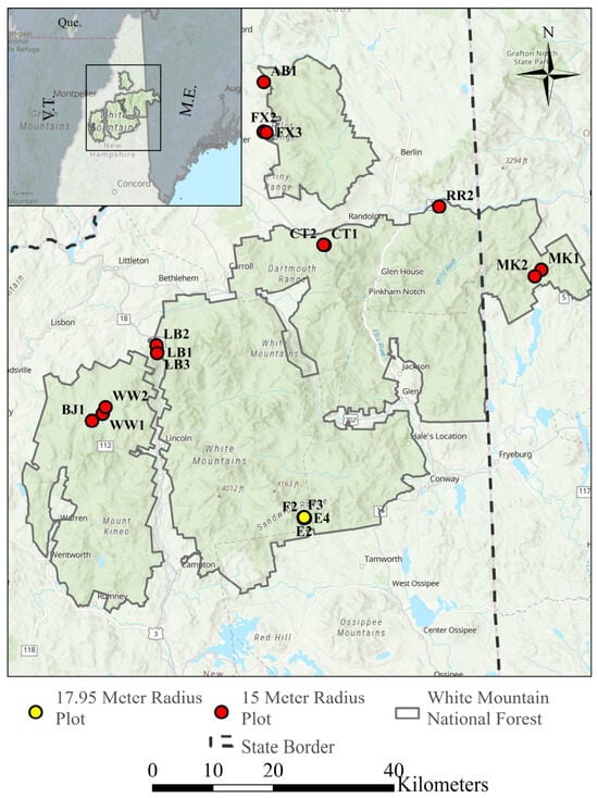
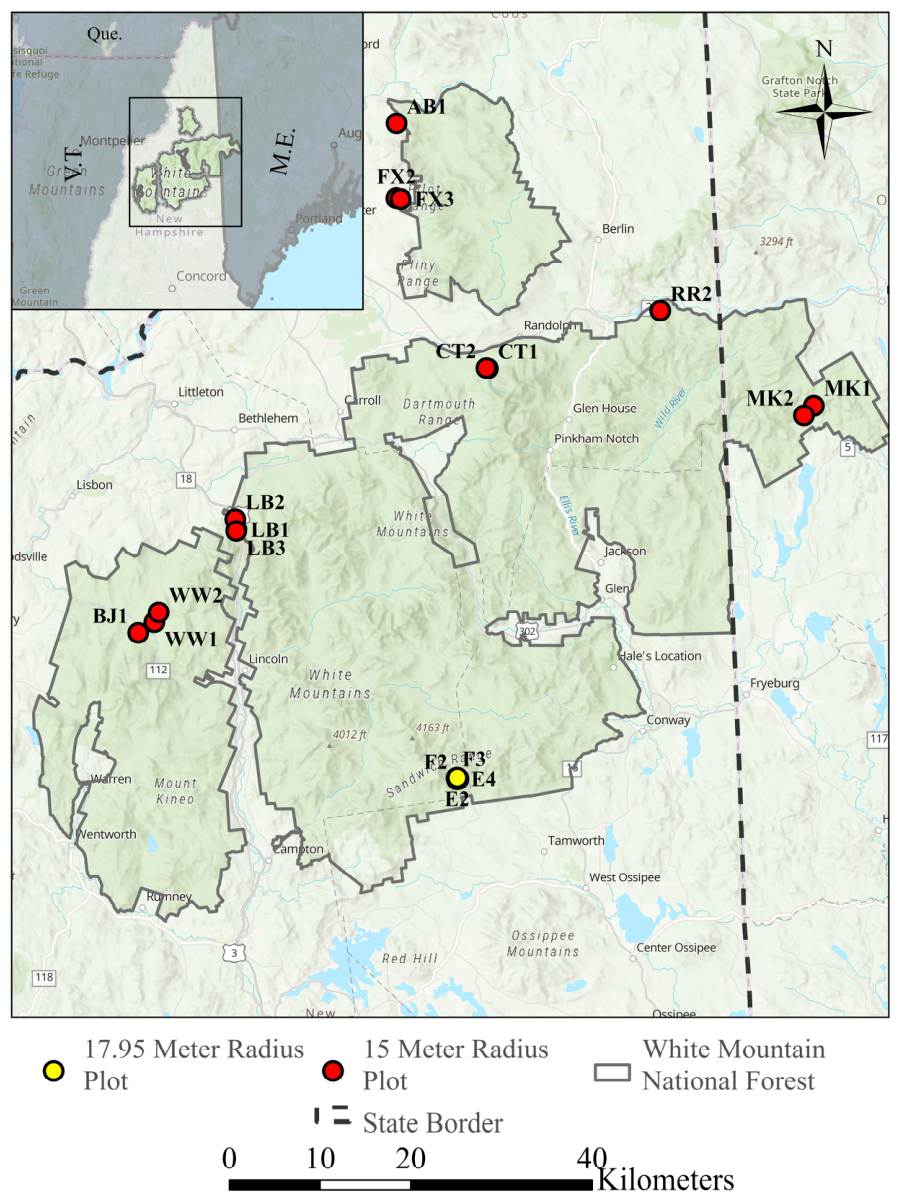
Samples were collected across the White Mountain National Forest (WMNF) in New Hampshire (approx. 44.0223°N, 71.4902°W) (Figure 1). Elevation within the WMNF ranges from approximately 440 m to 1900 m above sea level. The region is characterized by a humid continental climate, experiencing four distinct seasons, with snowy, dry winters and warm, humid summers. Average winter and summer temperatures of −7 °C (19 °F) and 21 °C (70 °F), respectively. Annual precipitation averages between 400 and 850 mm (16 in to 35 in), with a significant portion falling as snow [17].
Figure 1.
Plots are located within the White Mountain National Forest. Labels such as AB1, BJ1, CT1, etc., are representative of plot names. Coordinates approx. 44.0223°N, 71.4902°W.
The WMNF forms part of the broader “Northern Forest” ecosystem, which is dominated by northern hardwood species at lower elevations and boreal species at higher elevations and farther north. Species composition at lower elevations primarily includes Acer saccharum (sugar maple), Betula alleghaniensis (yellow birch), Fagus grandifolia (American beech), Fraxinus americana (white ash), Pinus strobus (white pine), and Tsuga canadensis (eastern hemlock). At higher elevations, the forest transitions to dominance by Abies balsamea (balsam fir), Picea glauca (white spruce), Picea mariana (black spruce), and Picea rubens (red spruce) [18,19].
2.2. Plot Selection
Plots used in this study consisted of thirteen 15 m radius and four 17.95 m radius plots (Figure 1). These plots were selected from a larger pool of 51 total plots associated with two ongoing studies. A total of 35 15 m radius plots focused on decadal tree growth in managed forests, while a total of 16 17.95 m radius plots focused on similar growth patterns in old-growth stands. For both plot types, all trees with a DBH ≥ 5 cm were measured. In the 17.95 m radius plots, a nested 5.7 m subplot was also established to record smaller trees with a DBH between 2.5 cm and 12.5 cm, while trees greater than 12.5 cm were measured across the full 17.95 m plot.
From this pool, a subset from each study was selected based on its suitability for MLS. Plots were excluded where field conditions limited safe or effective scanner operation, including dense understory vegetation that restricted transect movement or substantially, as well as physical obstacles such as low branches that posed a risk of contact with the sensor. This selection reflects operational constraints of MLS systems, where forest characteristics such as understory density and structural complexity can directly influence the feasibility of scanning. In this study, several plots were excluded due to these physical limitations, highlighting a key constraint of MLS deployment in more structurally complex forest environments.
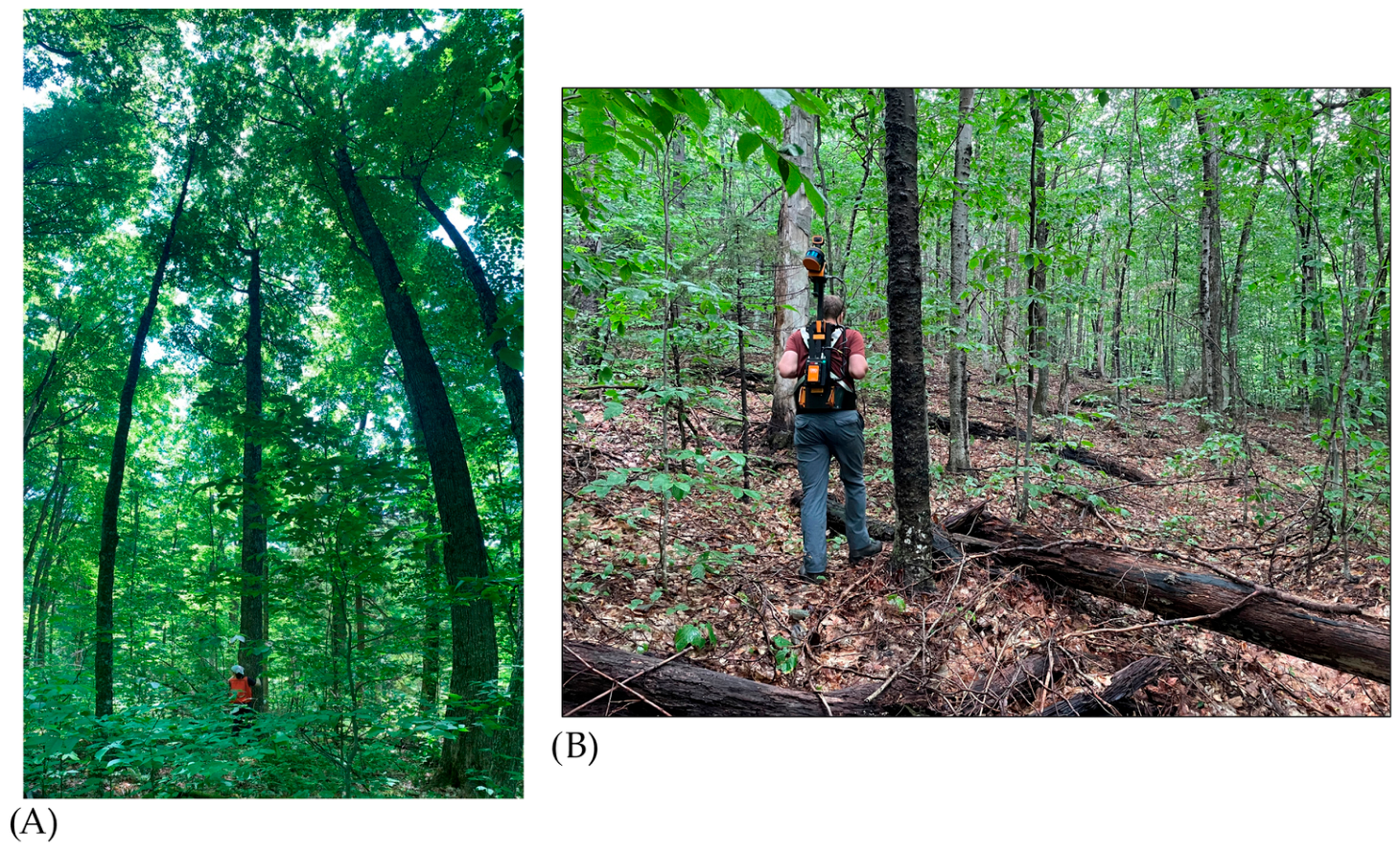
These plots, although varying in topography and forest structure, tended to host similar tree species with dominant trees being yellow birch, American beech, sugar maple, and white ash (Figure 2). Site conditions ranged from even-aged and flat topography to uneven-aged and hilly terrain, with a variety of intermediate conditions. Plots were also situated across a range of slope aspects, including north-, south-, east-, and west-facing slopes.
Figure 2.
Examples of forest characteristics scanned across the 17 plots and the scanner being used. (A) Field measurements being conducted at a plot; (B) Scanning in action of a plot.
2.3. Reference Data Acquisition
A total of 17 plots were hand-measured for reference data, with 3 plots collected in the summer of 2023 and 14 measured in the summer of 2024. Reference data entailed measuring tree distance and azimuth using a hypsometer and compass from the plot center and DBH measurements of trees at a minimum of 5 cm. Measurements for all trees were done within the designated radius of the plots. Additionally, each tree received a unique identification number.
2.4. GeoSLAM Zeb Horizon Specifications and Data Acquisition
The mobile LiDAR system used was the GeoSLAM Zeb Horizon (FARO Technologies, Lake Mary, FL, USA) [20]. The Zeb Horizon is a mobile unit that can be handheld or backpack-mounted and shoots at a wavelength of 903 nm with the integrated SLAM algorithm. Its maximum scanning range is a maximum of 100 m with a scan rate of 300,000 points per second, with a horizontal angular resolution of 0.20° (Table 1).
Table 1.
GeoSLAM Zeb Horizon specifications.
Scanning was conducted during the summer of 2024 under leaf-on conditions. This timing reflects typical forest inventory applications in the Northern Forest, where winter conditions limit access and the leaf-off period in spring and fall is relatively short.
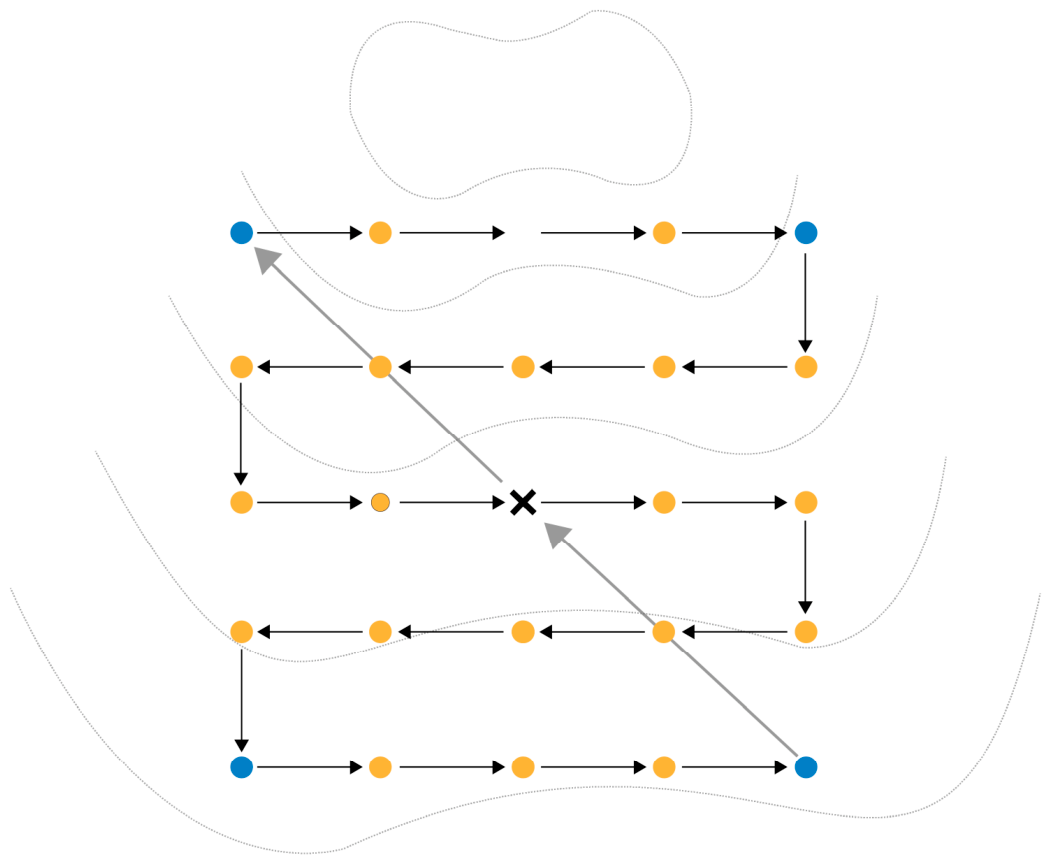
Each radius plot was overlaid with a 40 m × 40 m grid scanning path. This would ensure that each plot was scanned in its entirety with overlap, thus ensuring no missing portions of the plot (Figure 3). Scanning would typically start in the uphill corner of the 40 m grid and run serpentine across five transects spaced 10 m apart to the opposite downhill corner. Additionally, at each plot corner and plot center, the walking would pause while scanning to create “benchmark” locations. These benchmarks allow for easy visualization of plot corners. The scanning path would be concluded by walking diagonally across the plot to the uphill starting position, to close the loop of the scan according to the system scanning guidelines. Scanning speed was conducted at a slow, consistent walking pace (~0.5–1.0 m s−1), with the sensor maintained at an approximate height of 1.9 m above ground in an upright orientation. Lastly, the data would be immediately downloaded from the system’s data logger to a field computer.
Figure 3.
The 40 × 40 m scanning path for LiDAR on a hillside, with scanning starting in the uphill corner. Lines represent hypothetical scanning path in accordance with scanning protocol. Dots represent 10 m locations marked in the field for navigation.
2.5. Data Preprocessing and Segmentation
LiDAR point cloud data was processed into .las files using the FARO Connect software (version 2024.3.5) [20]. To refine the point clouds to their respective plots, spatial clipping was performed using the lidR 4.2.1 package in R [21] by calculating the point cloud centers and providing a buffer of 18 m for the 15 m plots and a 21 m radius for the 17.95 m radius plots to ensure proper overlap of the true plot center with the point cloud center.
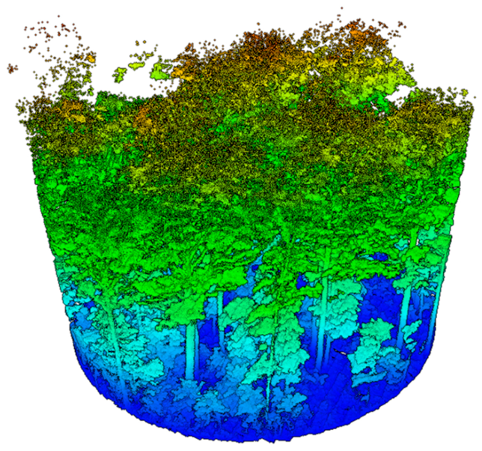
Once point clouds were clipped to approximate plot boundaries, ground points were identified using the default parameters of the cloth-simulation filter (CSF), implemented in the lidR 4.2.1 package [22]. A raster-based Digital Terrain Model (DTM) was generated using a 1 m grid resolution with elevation interpolated via the k-nearest neighbors algorithm. Finally, the point clouds were normalized by subtracting all ground elevation from the z-values of each point (Figure 4). This normalization provided a consistent ground-relative height surface across all plots, enabling accurate structural calculations.
Figure 4.
Plot AB1 preprocessed point cloud clipped to 15 m plot radius.
Segmentation of trees from the point clouds was conducted using the software CloudCompare 2.13.2 using the 3-D Forest Inventory (3DFIN) 2.13.1 plug-in [23,24,25]. Within the plug-in, parameters were adjusted under the “basic” settings menu, allowing control over the upper and lower stripe limits used to detect tree stems, as well as pruning intensity based on how much understory is found within each plot. According to the 3DFIN manual, the two stripe limits should be set to provide sufficient vertical distance between the two thresholds, ensuring the algorithm has enough space to accurately detect tree stems. For the lower stripe limit, a value of 1.3 m was used, corresponding to the standard height for DBH measurements and selected to minimize interference from understory vegetation. To establish an appropriate upper limit, a simple predictive height equation derived from tree slenderness was used to estimate total tree height [26]. The height of the shortest tree among these predictions was then used as the upper stripe threshold. This approach was intended to reduce the inclusion of extraneous points from understory vegetation and minimize potential misidentification of trees during the segmentation process. Across all the plots, a minimum predicted height of approximately 4.0 m was consistent with a maximum of up to 4.2 m.
The pruning height parameter within the algorithm is designed to account for noise within the point cloud caused by extraneous branching, interference from understory vegetation, and other potential sources of error that may lead to misidentification of trees. This setting operates on a scale of 1–5, with 1 representing minimal interference from noise or a relatively “clean” forest structure, and 5 indicating a very dense and structurally complex forest environment. For all plots in this study, a pruning intensity of 4 was selected to reflect the high structural complexity observed across the sites.
Following segmentation, the identity of segmented trees was matched to those in the reference field data, and coordinate systems were aligned within a relative plot-based coordinate framework. Quantile regression (which is robust to outliers) was then applied to account for systematic offsets between LiDAR-derived and reference coordinates, ensuring that residual misalignment did not bias tree detection statistics. In essence, our approach substituted a least absolute deviation error criterion (i.e., that used in quantile regression) for the least square criterion used in the conventional iterative closest point (ICP) algorithm, and thus would be more robust to outlying position errors should any be present. Once matching reference trees and segmented trees were aligned, a distance filter of 15 m for the 15 m plots and 17.95 m for the 17.95 m plots removed any added segmented trees that fell outside of the measured plot boundaries. Additionally, for the 17.95 m plots, a distance of 5.7 m was used for trees with DBH between 5 cm and 12.7 cm, to match the field protocol for including small-diameter trees.
2.6. Statistical and Structural Analysis
2.6.1. Tree Detection Accuracy Results
To evaluate detection accuracy at both the plot level and across all plots, two standard metrics, recall and precision, were calculated using the counts of True Positives (TPs), False Positives (FPs), and False Negatives (FNs). Recall was calculated as
Precision was calculated as
These metrics quantify different aspects of detection performance: recall measures the proportion of reference trees correctly detected, while precision measures the proportion of segmented trees that correspond to actual reference trees. It is also important to note that the inverse of these metrics provides omission and commission rates, respectively.
To provide a combined measure of detection performance, the F1-score was also calculated:
The F1-score balances the trade-off between omission and commission errors, providing a single metric that reflects overall detection performance.
2.6.2. Plot-Level Characteristics
To understand the structure and variation in the plots, five metrics were calculated: basal area per ha (BA, m2/ha), quadratic mean diameter (QMD, cm), relative stand density (RD, unitless), proportion softwood (unitless), and total tree density (trees/ha).
Basal area per hectare was calculated as
where is the basal area of each individual tree and is the plot area in hectares.
Quadratic mean diameter (QMD) was calculated as
where is the diameter at breast height (cm) and is the number of trees in the plot.
Tree density was calculated as
The contribution of each tree to relative stand density (RD) was calculated following Ducey and Knapp [27]:
where is the expansion factor (trees per hectare), is wood specific gravity, and is the diameter at breast height. Plot-level relative density was calculated as
The proportion of softwood was calculated as the ratio of softwood trees to the total number of trees within each plot.
For subsequent regression analysis, variables were scaled to improve numerical stability. This transformation centered each variable by subtracting the mean and dividing by its standard deviation, resulting in a mean of 0 and a standard deviation of 1. This ensured that predictors with different magnitudes contributed appropriately to model estimation.
2.6.3. Equivalency Test
To assess the comparability of segmented data to reference data, an equivalency test was conducted for both tree density and basal area using the equivalence package in R [28,29]. Unlike traditional hypothesis testing, which evaluates for significant differences, equivalence testing evaluates whether differences are small enough to be practically negligible—thus allowing for validation of similarity rather than dissimilarity.
A two one-sided t-test (TOST) was employed with a 90% confidence interval to determine whether the segmented estimates fell within pre-defined equivalence margins of ±10% for tree density and ±10% for basal area per hectare. If the entire confidence interval of the difference lies within these margins, the null hypothesis of dissimilarity is rejected, indicating statistical equivalence between segmented and reference data.
2.6.4. Tree Detection Logistic Regression with Mixed-Effect Models
To analyze the first objective, the effectiveness of tree detection, two separate logistic regression models with mixed effects were employed. These models assessed the predicted probability of either correctly identifying the presence of a tree within the point cloud or mistakenly detecting a tree where none exists. Specifically, we evaluated two scenarios: (1) the probability that a reference tree had a corresponding segmented tree (recall); and (2) the probability that a segmented tree had a corresponding reference tree (precision).
These two models ask two distinct, but related, questions. The recall model examines the detection of real, field-measured trees within the segmented data, while the precision model investigates whether segmented trees correspond to actual trees in the reference dataset. These two detection outcomes are inversely related to omission and commission errors. If a reference tree lacked a corresponding segmented tree, it was considered an omission (missed detection). Conversely, if a segmented tree lacked a corresponding reference tree, it was considered a commission (false detection). This modeling framework allowed for the quantification of detection accuracy and the identification of factors influencing both types of error.
In both analyses, DBH from the reference dataset served as the primary fixed effect to determine whether tree size influences detection accuracy. Plot identity was included as a random effect to account for unmeasured plot-level variation that might influence tree detection. Additional plot-level covariates—basal area (BA), quadratic mean diameter (QMD), relative stand density (RD), proportion softwood, and tree density—were also incorporated to evaluate their impact on tree detection probability and evaluate whether their inclusion improved model fit. Model comparison was conducted using Akaike Information Criterion (AIC) values. The following model was used to assess the probability that a reference tree had a corresponding segmented tree (recall model):
In this model, Pij represents the predicted probability of detection for the ith tree in the jth plot. The term DBHref, ij denotes the diameter at breast height of each reference tree. The fixed effect coefficient β captures the relationship between DBH and detection probability, while α represents the model intercept. The term υj is a random intercept associated with plot j, accounting for unobserved plot-level variation, and εij is the residual error term representing tree-level deviation not explained by the fixed or random effects.
To evaluate whether segmented trees correspond to real trees (precision model), a structurally similar model was used, substituting the segmented tree DBH as the fixed effect:
Together, these models allowed for evaluation of both recall and precision, with DBH as a key predictor of detection accuracy and plot-level random effects included to account for variation among sampling locations. The model with the lowest AIC and BIC values was selected as the best-fitting model for assessing detection rates.
2.6.5. DBH RMSE
Root mean square error was calculated to quantify the average squared difference between reference and LiDAR-derived DBH estimates. RMSE provides a weight measure of model accuracy, penalizing larger errors more heavily. RMSE was calculated as
In this equation, yi represents the observed (true) value of the reference data, is the corresponding predicted value of the LiDAR-derived DBH, and n is the total number of matched observations.
Additionally, to contextualize the RMSE relative to the scale of the data, normalized RMSE was calculated as
where RMSE is the root mean square error between the reference and LiDAR-derived DBH values and is the mean DBH of the reference data.
2.6.6. DBH Equivalency Test
Similarly to tree detection, an equivalency test was conducted to evaluate if segmented DBH measurements are statistically equivalent to reference DBH measurements using the equivalence package in R [28]. A two one-sided t-test (TOST) was employed with a 90% confidence interval to determine whether the segmented estimates fell within pre-defined equivalence margins of ±2 cm. If the entire confidence interval of the difference lies within these margins, the null hypothesis of dissimilarity is rejected, indicating statistical equivalence between segmented and reference data.
2.6.7. Linear Regression with Mixed-Effect Models
To address the second objective, comparing segmented DBH measurements to real-world hand measurements, two linear mixed-effect regression models were performed. The first model predicted LiDAR-derived DBH from field-measured DBH, while the second (inverse) model assesses whether segmented DBH could accurately predict reference DBH values. Additionally, the same plot-level covariates used in the tree detection models were tested to determine whether stand characteristics influenced DBH prediction accuracy. The following model was used to predict LiDAR DBH:
where DBHseg is the response variable for the ith tree in the jth plot, α is the fixed intercept, β is the slope associated with DBH, and DBHref is the field-measured DBH for the ith tree and jth plot, is the random effect for each plot, and εij is the residual error.
An inverse model was also fitted using the same structure, with DBHseg as the predictor and DBHref as the response, to assess the bidirectional relationship between LiDAR and field measurements.
2.6.8. DBH Power Variance Function
To evaluate whether the accuracy of DBH predictions changed with tree size, a power variance function model was applied using the varPower structure in the nlme package in R [30,31]. The variance of the residuals is modeled as
where is the base residual variance, is the power parameter that is estimated from the data, and is the reference DBH for the ith tree in the jth plot. When = 0, the residual variance is constant, indicating that prediction accuracy is consistent across all DBH sizes. When > 0, residual variance increases with DBHref, suggesting that predictions are more variable for larger trees. When < 0, residual variances decrease with DBHref, suggesting that predictions are more variable for smaller trees.
3. Results
3.1. Tree Detection Accuracy
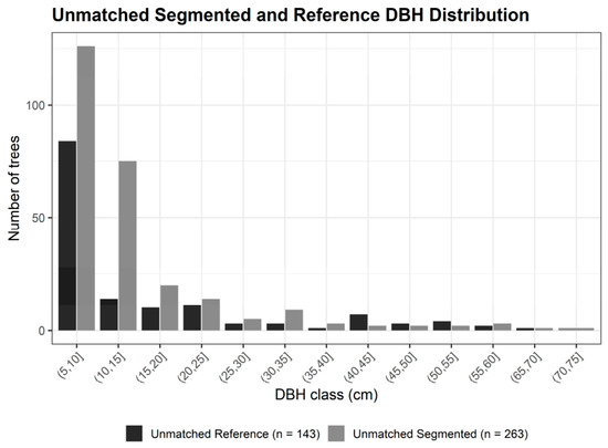
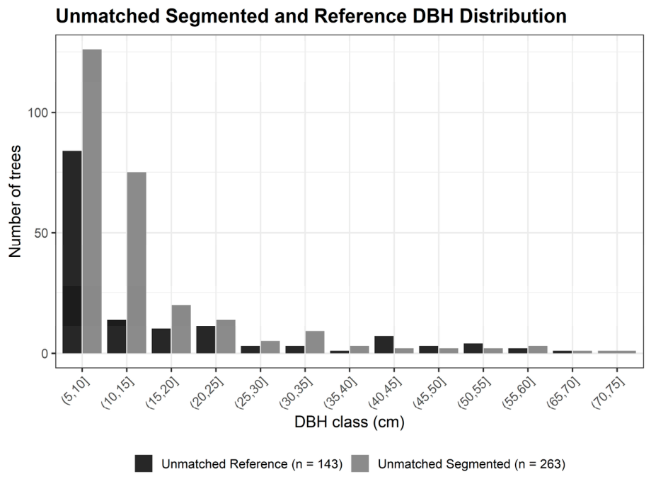
Across all plots, an overall recall rate (i.e., the detection rate of real trees) of 85.4% was achieved, with 14.6% of real trees omitted from the segmented dataset. Unmatched reference trees had a mean DBH of 14.6 cm (SD = 13.8) with a range between 5.0 cm and 69.8 cm, indicating that smaller trees were most omitted from detection (Figure 5). Further, after removing unmatched segmented trees below 5 cm, the proportion of segmented trees matched to real trees was 74.0%, indicating a 26.0% false positive rate. However, it is important to note that some large trees (up to 69.8 cm DBH) were also omitted, suggesting that omission errors were not limited to small diameter stems and, in some cases, involved larger trees as well. Unmatched segmented trees had a mean DBH of 13.9 cm (SD = 11.3 cm) with values ranging from 5.0 cm to 73.3 cm, showing that most false positive trees were smaller in diameter (Figure 4). Notably, 103 false positive trees under 5 cm in DBH were present prior to filtering. Together, these results yielded an F1-score of 0.81, indicating a strong balance between omission and commission errors.
Figure 5.
Distribution of unmatched reference and segmented trees by DBH. Both distributions indicate that smaller trees are more likely to be falsely added and omitted through the segmentation process.
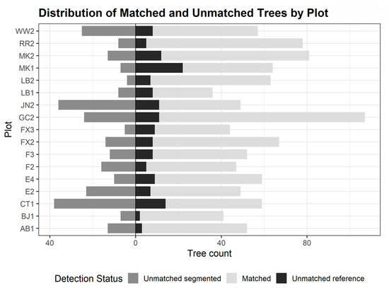
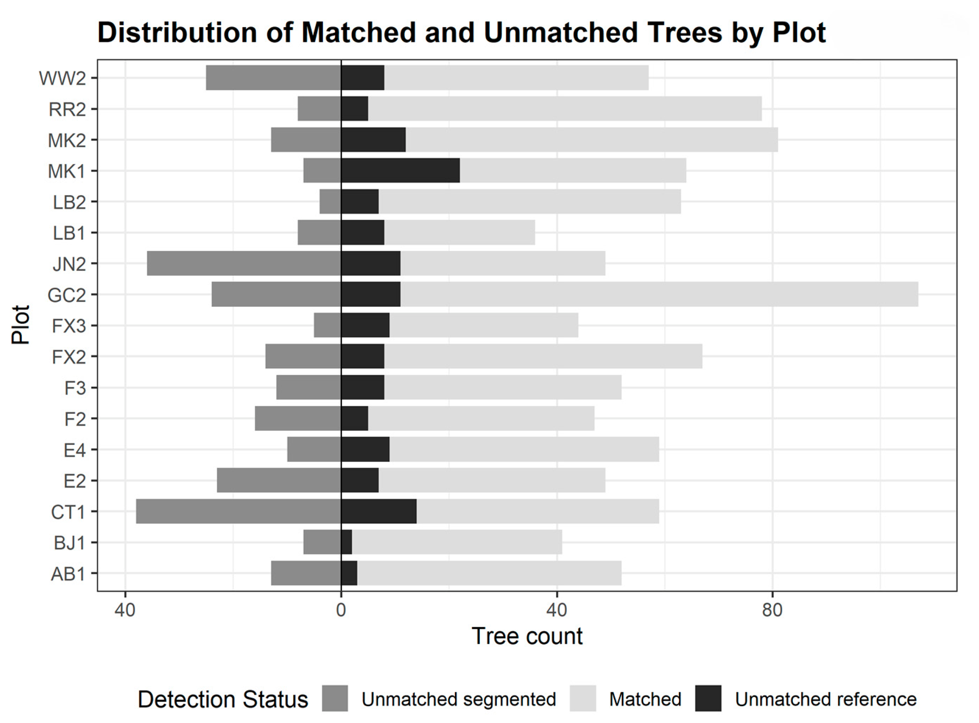
At the plot level, the number of matching trees ranged from 27 to 95, with an average of 49.9 per plot. This left unmatched reference trees with a minimum of 2, a maximum of 22, and an average of 8.7. Unmatched segmented trees ranged from 5 to 39, with an average of 16.9 (Figure 6).
Figure 6.
Plot-level breakdown of tree detection outcomes, including matched trees, unmatched reference trees, and unmatched segmented trees.
3.2. Plot-Level Summary Statistics
The analysis summarized stand-level metrics for all 17 plots. Table 2 presents the total number of matching trees, unmatched reference trees, unmatched segmented trees, and the corresponding detection, omission and commission rates for each plot. This table emphasizes the variability in detection performance by illustrating how many real trees were missed and how many false trees were added through segmentation. Table 3 shows plot-level stand metrics calculated for both reference and LiDAR-segmented trees. Both tables highlight the variability in detection rates per plot and their associated physical characteristics.
Table 2.
Plot-level tree detection results for all 17 plots. Metrics include total reference trees, total matching trees, unmatched reference trees, and unmatched segmented trees. These values show variability in the plot of detection results across the plots.
Table 3.
Plot-level stand metrics for the 17 sample plots. Metrics include tree density (trees/ha), basal area (BA), and quadratic mean diameter (QMD) for both reference (Ref) and LiDAR-segmented (Seg) trees. Also included are plot-level values for the proportion of softwood species per hectare and relative density. Trees/ha difference is the difference in segmented trees/ha compared to reference trees/ha.
3.3. DBH Summary Statistics and Accuracy Metrics
Summary statistics were calculated for all trees across reference and LiDAR DBH measurements (Table 4). The mean DBH of the reference data was 19.8 cm (SD = 14.44 cm). The mean DBH for the LiDAR data was 19.7 cm (SD = 13.76 cm). The median values of both 14.7 cm indicate an equal relationship between LiDAR and field measurements. Minimum and maximum measurements were comparable, with both measurements capturing diameters up to approximately 108 cm. These statistics suggest that while LiDAR captures the general DBH distribution well, it tends to slightly underestimate DBH at the individual tree level.
Table 4.
Summary statistics for DBH measurements.
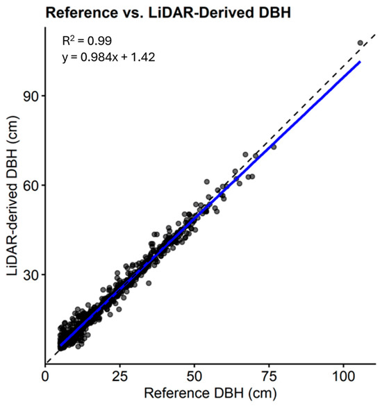
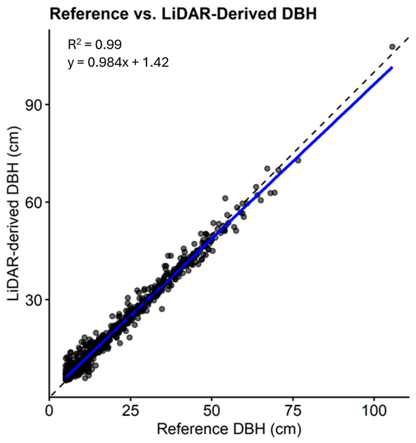
Among the 859 matched trees with both field and LiDAR DBH measurements, agreement between the two methods was strong (Table 5). The mean difference between the LiDAR and reference measurements was 0.36 cm. The RMSE was 1.98 cm (9.65%), reflecting the typical magnitude of error. The Pearson correlation coefficient between field and LiDAR DBH was 0.99, which indicates an exceptionally strong positive linear relationship between the two measurements (Figure 7).
Table 5.
DBH accuracy metrics between reference and segmented tree data by plot and with total (n = 859). RMSE “Small” Trees represents RMSE of trees between 5 cm and 25 cm. RMSE “Large” Trees represents RMSE of trees greater than 25 cm.
Figure 7.
Linear regression comparing field-measured DBH to LiDAR-segmented DBH.
To further examine variability in DBH estimation, Table 5 also presents these metrics at the plot level, along with values stratified by tree size class. RMSE for smaller trees (5–25 cm DBH) and larger trees (>25 cm DBH) is reported to assess how error varies with tree size. Across plots, RMSE for larger trees was generally higher than for smaller trees. Despite this, strong correlations were maintained across all plots, demonstrating consistent agreement between LiDAR-derived and field-measured DBH across varying stand conditions.
3.4. DBH, Basal Area, and Tree Density Equivalency Tests
To assess whether DBH measurements derived from the segmented data were statistically equivalent to reference measurements, an equivalency test was performed. The 90% CI for the mean difference was [0.270, 0.442], while the predefined margin was ±2 cm. The observed mean difference was 0.356 cm. Because the entire confidence interval lies within the equivalency bounds, the null hypothesis of non-equivalence was rejected, indicating that segmented DBH measurements are statistically equivalent to reference DBH values. The margin of ±2 reflects common field measurement variability and is consistent with error rates in forest inventory work, as well as providing leniency suitable for evaluating LiDAR-based measurements. However, it may not be sufficient for inventories designed to measure forest growth (cite Kershaw et al. [26]).
An equivalency test was also conducted to compare basal area per hectare estimates between reference and segmented datasets. The 90% confidence interval (CI) for the mean difference was [−1.54, 0.68], while the predefined equivalency margin was ±2.8 m2/ha. The observed mean difference between the two datasets was 0.25 m2/ha. Because the confidence interval lay within the equivalency bounds, the null hypothesis of non-equivalence was rejected, indicating that basal area estimates derived from segmented trees were statistically equivalent to those from the reference measurements.
Additionally, an equivalency test was conducted for tree density between the two datasets. The 90% CI for the mean difference was [−52.87, 49.13] trees ha−1, which lay entirely within the predefined equivalence margin of ±86.62 trees ha−1, or 10% of the mean. Because the confidence interval fell within the equivalence bounds, the null hypothesis of non-equivalence was rejected, indicating that tree density estimates derived from segmented trees were statistically equivalent to the reference measurements under the specified margin.
3.5. Reference Logistic Mixed Effects Model
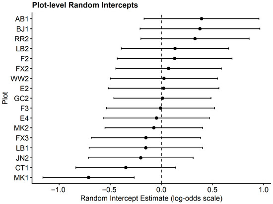
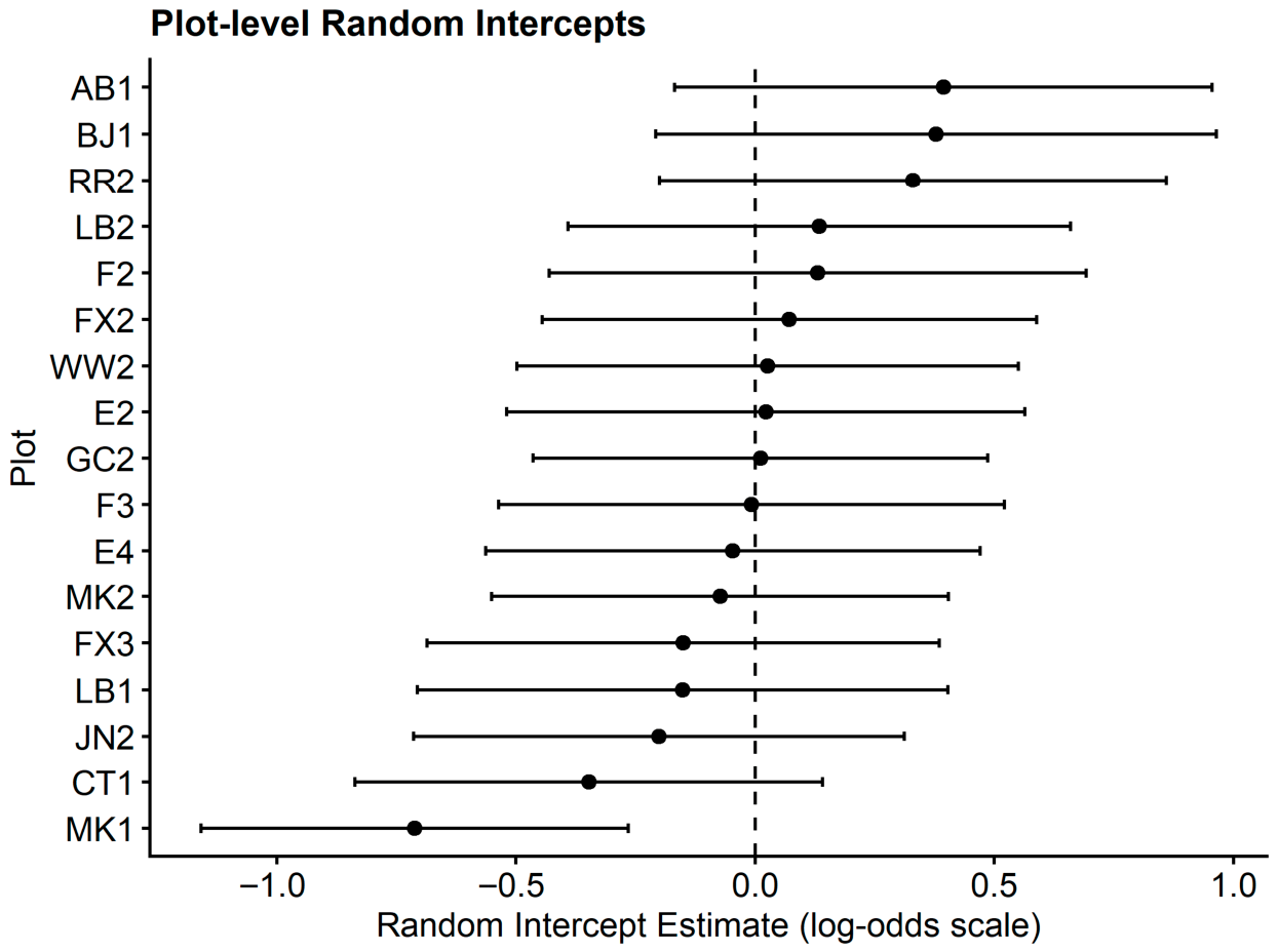
A logistic mixed effects model was used to determine the influence of five covariates on the probability of detection based on the DBH of the reference trees. Substantial variation in detection rates among plots justified the inclusion of plot as a random effect, along with plot-level covariates aimed at explaining inter-plot variability in detection performance (Figure 8).
Figure 8.
Random intercepts for tree detection by plot. Values greater than 0 indicate plots with a higher baseline probability of tree detection, while values less than 0 indicate lower detection probability relative to the overall average. Lines represent 95% confidence intervals.
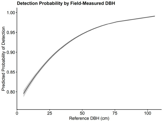
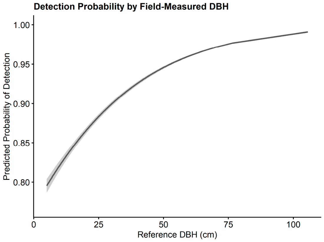
To assess model performance, six nested models were compared using the Akaike Information Criterion (AIC). The model with the lowest AIC was selected as the best-fitting model (Table 6). The best-fit model included DBH and stem density. In this final model, detection probability increased with reference DBH, suggesting that larger trees were more likely to be detected by the circle fitting algorithm. For every 1 cm increase in reference tree DBH, the odds of being detected by the LiDAR segmentation algorithm increased by ~3% (Figure 9). Higher stem density was associated with an increase in detection probability, although the effect was weak, with an increase of 100/trees per acre corresponding to a 9% increase in detection probability.
Table 6.
AIC values of reference logistic mixed effects model by adding single plot-level covariates.
Figure 9.
Probability of detection as a function of reference DBH. Shaded areas represent 95% confidence intervales.
3.6. Logistic Mixed-Effects Model Using Segmented Trees
Similarly to the previous model, a logistic mixed-effects model was used to evaluate the influence of plot-level covariates on the probability of a segmented tree corresponding to a real (reference) tree. Variation in matching rates among plots justified the inclusion of plot as a random effect. To assess model performance, six nested models were compared using AIC. The best-fit model included segmented DBH and relative density (RD) (Table 7). In this final model, the probability of a segmented tree corresponding to a reference tree increased with DBH, indicating that larger segmented trees were more likely to represent real trees. Relative density also had a positive effect on matching probability, suggesting more fully stocked stands were associated with slightly increased matching success.
Table 7.
AIC values of adding single plot-level covariates.
3.7. DBH Linear Regression
A linear mixed effects model was used to predict segmented tree DBH from reference DBH measurements, incorporating plot as a random intercept to account for plot-level variation. Two complementary modeling approaches were considered: the first involved sequentially adding plot-level covariates to evaluate their explanatory power at the plot scale, while the second focused solely on reference DBH and plot. This analysis included 849 pairs of matched trees across the 17 plots.
The model with the best fit, as indicated by the lowest AIC, was the simpler model that included only reference DBH as a fixed effect and plot as a random effect. In this model, segmented DBH increased with reference DBH (R2 = 0.95, df = 946.8). The fixed-effect slope indicated that for each additional centimeter in field-measured DBH, the predicted segmented DBH increased by approximately 0.95 cm, suggesting a slight underestimation by the segmentation process, but demonstrating an almost one-to-one correspondence between field- and LiDAR-derived measurements (Figure 6). Additionally, the residual versus fitted values plotshowed a random scatter around zero, supporting model assumptions of linearity and constant variance. No major patterns or heteroscedasticity were observed, indicating that the model appropriately captured the relationship between reference and segmented DBH. This was further supported with the power variance function yielding a value close to zero ( = 0.048), further indicating that minimal change in residual spread with increasing DBH.
The random effect of plot had a standard deviation of 0.34 cm, indicating modest plot-to-plot variation in the relationship between field- and LiDAR-derived DBH. The remaining variability (SD = 1.77 cm) occurred at the tree level, reflecting individual tree or segmentation-level error.
4. Discussion
4.1. Tree Detection Performance
The detection rate observed in this study (85.2%) is consistent with previous research utilizing MLS in forested landscapes which has reported detection rates ranging from 43% to 99.48% (Supplementary Materials; Table S1). However, the commission rate found here (23.5%) was relatively high compared to other studies which range from approximately 0.6% to 31% (Supplementary Materials; Table S1). This elevated rate of false positives may be attributed to the structural complexity of the Northern Forest, which is characterized by dense stands of shade-tolerant species, both shrubs and trees, and significant vertical layering [18,32].
Although trees below 5 cm DBH were removed from the main detection analysis, a sensitivity check revealed that these smaller stems increased the commission rate from 23.5% to 30.3%, a 6.8% rise, further supporting the notion that dense understory vegetation may contribute to over-segmentation and misclassification. Gollob et al. (2020) reported a similar pattern, with commission errors increasing as the DBH detection threshold was lowered, although the magnitude of the effect was smaller than observed here [33]. These conditions are likely to increase the probability of both false positives and detection challenges.
It is also important to acknowledge the presence of a few, but notable, larger trees among both the omission and commission errors (Figure 4). Larger trees contribute disproportionately to ecosystem services and structural complexity, so their exclusion or erroneous inclusion introduces disproportionate error in forest estimates and stand characterization [34].
4.2. Influence of Forest Structure on Detection
To evaluate how forest structure influences detection performance, several plot-level covariates were incorporated into the models, including tree density, relative density (RD), basal area, QMD, and proportion of softwood. Overall, these structural attributes showed limited influence on detection probability, consistent with previous studies suggesting that MLS detection performance is driven more by individual tree size and completeness of stem coverage in the point cloud than stand-level composition alone [12,35]. Tree density had a marginal effect on detection probability, showing a slight improvement in model performance as tree density increased; however, as shown in previous studies, an increase in tree density may not necessarily lead to an increase in detection rates within different forest compositions [33]. In fact, previous studies have shown that an increase in tree density primarily leads to a decrease in detection accuracy [7,36].
RD showed a slightly improved model fit for predicting whether segmented trees correspond to real-world trees, with a positive effect on detection probability (Table 7). This relationship is likely influenced by the structural characteristics of the sampled plots, which exhibited a range of RD values typical of closed-canopy stands [37,38]. However, similar RD values can represent a range of forest structures, including stands with fewer, larger overstory trees that limit understory development, as well as denser, earlier successional stands composed of many smaller individuals. Additionally, higher overstory density may suppress understory vegetation, which could indirectly influence detection accuracy. As a result, the effect of RD observed in this study may not fully capture how different structural conditions associated with similar RD levels influence detection performance, particularly for smaller trees as observed in this study. Future research should evaluate whether comparable RD values across structurally distinct forest conditions produce consistent effects on detection outcomes.
These inconsistencies suggest that tree density, RD, or any of the other covariates examined in this study do not adequately explain plot-level variation in detection performance. One potential source of unexplained variability may lie in understory complexity and regeneration dynamics [26], which were not directly measured in this analysis. Specifically, the density and spatial frequency of certain shrub species or suppressed trees that fell below the minimum DBH threshold for inclusion (<5 cm) may influence segmentation outcomes and increase the risk of both omission and commission errors. Kükenbrink et al. (2022) reported no clear relationship between shrub presence and tree detection, but noted that the limited sample size constrained the strength of that conclusion, thus suggesting further testing should be performed [39].
In addition to low-lying vegetation, the presence of an intermediate canopy layer, composed of saplings or small overstory trees, may further complicate the segmentation process by introducing additional vertical overlap and occlusion within the point cloud. These structural features can challenge the ability of segmentation algorithms to differentiate individual stems, especially in dense, multi-layered forests. Inclusion of these features may decrease omission and commission rates further. Future studies should consider incorporating detailed understory vegetation metrics and species composition data to more fully understand sub-canopy and understory complexity influences MLS-based tree detection. Two additional plot-level factors that may affect detection accuracy are terrain slope and seasonal timing. Bauwens et al. (2016) noted that sloping terrain may alter the proximity of understory and branching structure to the scanner, potentially increasing omission and commission errors [40]. Additionally, all MLS scans in this study were conducted during leaf-on conditions, which likely contributed to increased occlusion. Oveland et al. (2018) similarly suggested that scans conducted during leaf-off conditions may improve visibility and segmentation accuracy, particularly in deciduous-dominated stands ([41]; see Kükenbrink). However, leaf-off scanning may prove restrictive. In our study region, much of the leaf-off period also coincides with snow, limiting access to plots in steep terrain and obscuring the ground, which would complicate the accurate determination of DBH.
4.3. Tree-Level Relationship
At the tree level, both logistic regression models demonstrated that detection accuracy increased with DBH. Larger trees, whether in the field dataset or the segmented output, had higher odds of being correctly matched. This suggests that tree size plays a key role in the visibility and successful segmentation of individual stems using mobile LiDAR. As shown by Lopez Serrano et al. (2022), complete coverage of an individual stem corresponds with increased detection probability; thus, larger trees having more surface area have better odds of complete coverage given a proper scanning path [42]. In contrast, when examining the proportion of unmatched reference and LiDAR-derived trees, trees with a smaller DBH were likely to be omitted from the segmented dataset or falsely added without a corresponding field match. This pattern further supports, both at the plot-level and individual tree level, that smaller trees and understory characteristics not measured in this study may impact detection accuracy, both by missing or incorrectly adding trees [39].
4.4. Implications for Forest Inventory Applications
These results underscore several important considerations for applying MLS in forest inventory contexts. First, the segmentation algorithm used in this study appears to overestimate tree counts at the plot level, likely due to noise and structural complexity—resulting in inflated estimates of forest structure and composition. To address this, additional preprocessing techniques [33] as well as employing a more refined segmentation process (i.e., using more refined settings and parameters) [43,44] may significantly reduce the influence of noise and complexity of understory vegetation on detection rates. Moreover, variation in segmentation performance across studies is not solely due to differences in forest conditions but also reflects the wide range of algorithms and techniques used to process point clouds. This highlights the need for continued evaluation, refinement, and ultimately standardization of segmentation methods, particularly within similar forest types, to optimize both tree detection and DBH estimation outcomes.
Second, although an 85.3% detection rate is relatively high, the omission of approximately 15% of real trees introduces bias in forest inventories, particularly because undetected trees result in systematic underrepresentation in forest inventories. Such omission can impact future analyses at the stand-level, including estimates of basal area, stand density, or biomass estimates, which were further highlighted in the equivalency tests. Lastly, the high commission rate (23.5%) will lead to overestimation of forest structural attributes, particularly stem density and other stand-level derived metrics, and must be accounted for when interpreting segmented data in applied forest monitoring or modeling efforts. Because both omission and commission errors are concentrated among smaller trees, metrics such as tree density are especially sensitive to these biases, whereas metrics like basal area, aboveground carbon estimates, and stand volume are less sensitive. Without a substantial reduction in commission error, full confidence in segmented results requires time-intensive field validation to confirm tree presence. Together, omission and commission errors introduce compounding biases into forest inventory estimates if not properly addressed.
4.5. Accuracy of DBH Measurements
For DBH measurements of segmented trees, the results showed a very strong relationship between LiDAR-derived and field-measured values. On average, segmented DBH differed from field-measured DBH by 0.36 cm, with an RMSE of 1.98 cm across individual trees. Over 859 matched trees, the correlation between LiDAR and field measurements was nearly perfect (R2 = 0.99), indicating that the segmentation process provides highly accurate DBH estimates across a range of tree sizes. Together, these results demonstrate low bias and limited variability between LiDAR-derived and field-based DBH measurements.
These findings are consistent with previous studies, which reported RMSE values for DBH estimation ranging from 1.11 cm to 6.26 cm (Supplementary Materials, Table S1; [40,45]). Although the segmentation process may overestimate tree presence and omit a fraction of actual trees, the quality of measurements for correctly identified trees is exceptionally high. In particular, the accuracy of DBH estimates implies that individual tree metrics derived from mobile LiDAR can be used confidently in forest structural assessments.
4.6. Operational Viability and Integration
This level of precision indicates the use of mobile LiDAR as a valuable addition to traditional field-based inventory methods in forests where scanning is logistically feasible. Despite strong performance in DBH estimation, the operational viability of MLS for stand-level inventory is currently limited by tree detection performance, particularly omission and commission errors. Until detection accuracy improves, MLS alone cannot fully replace conventional field inventories in complex, mixed-species forests.
While MLS shows promise, several traditional field measurements remain difficult to replicate, including the detection of smaller-diameter trees observed in this study. However, with continued refinement, MLS has clear potential as a complementary tool that expands the spatial scale and detail of forest inventory when integrated with traditional field sampling [13,46,47]. Until more reliable tree detection methods are implemented, combining larger spatial-scale scans with nested-plot hand measurements of smaller diameter trees may provide a practical approach to capturing underrepresented attributes while leveraging the strengths of MLS.
Lastly, sample selection was limited in this study due to hazards that posed risks to the equipment. This practical limitation introduces bias when characterizing forest systems; however, it also reflects how MLS systems are likely to be deployed in operational settings with similar structural conditions. Future research could explore how model-based or hybrid inference might be used to address practical limitations for MLS, as discussed by Saarela et al. (2017) in the context of vehicle-mounted mobile scanning [48]. This issue further highlights the need to integrate MLS with traditional field sampling, or with the use of other covariates such as those derived from airborne or drone-based LiDAR. Finally, as MLS hardware evolves, we may hope that future designs offer more robust protection from scratches and impacts to the sensor and other system components.
5. Conclusions
This study served as a preliminary assessment of the effectiveness of MLS in complex, mixed-species forest conditions and characteristics of the northeastern United States. Specifically, it evaluated the ability of MLS to detect individual trees and accurately estimate DBH in mixed-species forest environments. An overall detection rate of 85.2% and a commission rate of 23.5% were observed, alongside a DBH estimation RMSE of 1.98 cm.
These findings point to two key future considerations: (1) while MLS-derived point clouds show potential for forest inventory applications, refinement of the segmentation process is needed to reduce false positives and improve the accuracy of tree detection in complex forests; and (2) expanding this evaluation to include additional structural characteristics, such as understory shrubs and regeneration, would help clarify the forest conditions under which MLS is most effective.
Despite limitations in detection performance, DBH estimates for correctly identified trees were highly accurate with strong agreement with field measurements. This indicates that if detection performance can be further improved, particularly by reducing omission and commission errors, MLS systems could become a reliable and efficient tool for operational forest inventory and structural analysis in mixed-species stands [49,50,51,52,53,54,55,56,57,58,59,60].
Supplementary Materials
The following supporting information can be downloaded at: https://www.mdpi.com/article/10.3390/rs18091382/s1. Supplementary Materials Table S1. Summary of previous studies evaluating tree detection and DBH measurements using MLS scanning. Studies span a range of geographic regions, forest types, and stand structures, highlighting the variability in stem density, species composition, and sampling design. Forest structure and stem density values (stems/ha) are reported where available. Table adapted and expanded from Balenović et al. (2020) [13].
Author Contributions
Conceptualization, H.M. and M.J.D.; methodology, H.M.; software, H.M.; validation, M.J.D., B.T.F. and O.F.; formal analysis, H.M.; investigation, H.M.; resources, M.J.D.; data curation, H.M.; writing—original draft preparation, H.M.; writing—review and editing, H.M., M.J.D., B.T.F. and O.F.; visualization, H.M.; supervision, M.J.D.; project administration, M.J.D.; funding acquisition, M.J.D. All authors have read and agreed to the published version of the manuscript.
Funding
This research was supported by Cooperative Cost Share Agreement 20-CS-11092200-021, “LiDAR-Enabled Monitoring on the White Mountain National Forest,” and Joint Venture Agreement 17-JV-11242306045, “Old-Growth Forest Dynamics and Structure,” between the USDA Forest Service and the University of New Hampshire. Additional funding was provided by the New Hampshire Agricultural Experiment Station. This work (scientific contribution number 3088) was supported by the McIntire–Stennis program, project 00106-M (Accession Number 7003549), from the US Department of Agriculture’s National Institute of Food and Agriculture and the state of New Hampshire.
Data Availability Statement
The raw data supporting the conclusions of this article will be made available by the authors on request.
Acknowledgments
We thank the USDA Forest Service for the use and access to plots within the White Mountain National Forest (WMNF) used in this study. Specifically, we are grateful to Scott Bailey for the establishment and use of the research plots. We thank Dakota Mako and Sally Pizzuto for their efforts in field and LiDAR data collection.
Conflicts of Interest
The authors declare no conflicts of interest.
Abbreviations
The following abbreviations are used in this manuscript:
| LiDAR | Light Detection and Ranging |
| DBH | Diameter at Breast Height |
| ALS | Aerial Laser Scanning |
| TLS | Terrestrial Laser Scanning |
| MLS | Mobile Laser Scanning |
| SLAM | Simultaneous Localization and Mapping |
| RMSE | Root Mean Square Error |
| CSM | Cloth-Simulation Function |
| DTM | Digital Terrain Model |
| BA | Basal Area |
| QMD | Quadratic Mean Diameter |
| RD | Relative Density |
| TPs | True Positives |
| TNs | True Negative |
| FPs | False Positives |
References
- Filotas, E.; Parrott, L.; Burton, P.J.; Chazdon, R.L.; Coates, K.D.; Coll, L.; Haeussler, S.; Martin, K.; Nocentini, S.; Puettmann, K.J.; et al. Viewing Forests through the Lens of Complex Systems Science. Ecosphere 2014, 5, art1. [Google Scholar] [CrossRef] [Scilit]
- Pretzsch, H.; Bauhus, J.; Forrester, D. Mixed-Species Forests, 1st ed.; Springer: Berlin/Heidelberg, Germany, 2017; ISBN 978-3-662-54551-5. [Google Scholar]
- Vatandaslar, C.; Boston, K.; Ucar, Z.; Narine, L.L.; Madden, M.; Akay, A.E. Precision Forestry Revisited. Remote Sens. 2025, 17, 3465. [Google Scholar] [CrossRef] [Scilit]
- Akay, A.E.; Ouz, H.; Karas, I.R.; Aruga, K. Using LiDAR Technology in Forestry Activities. Environ. Monit. Assess. 2009, 151, 117–125. [Google Scholar] [CrossRef] [Scilit]
- Kelly, M.; Di Tommaso, S. Mapping Forests with Lidar Provides Flexible, Accurate Data with Many Uses. Calif. Agric. 2015, 69, 14–20. [Google Scholar] [CrossRef] [Scilit]
- Narine, L.L.; Popescu, S.; Neuenschwander, A.; Zhou, T.; Srinivasan, S.; Harbeck, K. Estimating Aboveground Biomass and Forest Canopy Cover with Simulated ICESat-2 Data. Remote Sens. Environ. 2019, 224, 1–11. [Google Scholar] [CrossRef] [Scilit]
- Chen, S.; Liu, H.; Feng, Z.; Shen, C.; Chen, P. Applicability of Personal Laser Scanning in Forestry Inventory. PLoS ONE 2019, 14, e0211392. [Google Scholar] [CrossRef] [Scilit]
- Barbeito, I.; Dassot, M.; Bayer, D.; Collet, C.; Drössler, L.; Löf, M.; del Rio, M.; Ruiz-Peinado, R.; Forrester, D.I.; Bravo-Oviedo, A.; et al. Terrestrial Laser Scanning Reveals Differences in Crown Structure of Fagus sylvatica in Mixed vs. Pure European Forests. For. Ecol. Manag. 2017, 405, 381–390. [Google Scholar] [CrossRef] [Scilit]
- de Conto, T.; Olofsson, K.; Görgens, E.B.; Rodriguez, L.C.E.; Almeida, G. Performance of Stem Denoising and Stem Modelling Algorithms on Single Tree Point Clouds from Terrestrial Laser Scanning. Comput. Electron. Agric. 2017, 143, 165–176. [Google Scholar] [CrossRef] [Scilit]
- Huang, H.; Tang, L.; Chen, C. A 3D Individual Tree Modeling Technique Based on Terrestrial LiDAR Point Cloud Data. In Proceedings of the 2015 2nd IEEE International Conference on Spatial Data Mining and Geographical Knowledge Services (ICSDM), Fuzhou, China, 8–10 July 2015; IEEE: Piscataway, NJ, USA, 2015; pp. 152–156. [Google Scholar]
- Zhou, S.; Kang, F.; Li, W.; Kan, J.; Zheng, Y.; He, G. Extracting Diameter at Breast Height with a Handheld Mobile LiDAR System in an Outdoor Environment. Sensors 2019, 19, 3212. [Google Scholar] [CrossRef] [Scilit]
- Del Perugia, B.; Giannetti, F.; Chirici, G.; Travaglini, D. Influence of Scan Density on the Estimation of Single-Tree Attributes by Hand-Held Mobile Laser Scanning. Forests 2019, 10, 277. [Google Scholar] [CrossRef] [Scilit]
- Balenović, I.; Liang, X.; Jurjević, L.; Hyyppä, J.; Seletković, A.; Kukko, A. Hand-Held Personal Laser Scanning: Current Status and Perspectives for Forest Inventory Application. Croat. J. For. Eng. 2021, 42, 165–183. [Google Scholar] [CrossRef] [Scilit]
- Liang, X.; Kankare, V.; Hyyppä, J.; Wang, Y.; Kukko, A.; Haggrén, H.; Yu, X.; Kaartinen, H.; Jaakkola, A.; Guan, F.; et al. Terrestrial Laser Scanning in Forest Inventories. ISPRS J. Photogramm. Remote Sens. 2016, 115, 63–77. [Google Scholar] [CrossRef] [Scilit]
- Yrttimaa, T.; Saarinen, N.; Kankare, V.; Hynynen, J.; Huuskonen, S.; Holopainen, M.; Hyyppä, J.; Vastaranta, M. Performance of Terrestrial Laser Scanning to Characterize Managed Scots Pine (Pinus sylvestris L.) Stands Is Dependent on Forest Structural Variation. ISPRS J. Photogramm. Remote Sens. 2020, 168, 277–287. [Google Scholar] [CrossRef] [Scilit]
- Ryding, J.; Williams, E.; Smith, M.J.; Eichhorn, M.P. Assessing Handheld Mobile Laser Scanners for Forest Surveys. Remote Sens. 2015, 7, 1095–1111. [Google Scholar] [CrossRef] [Scilit]
- Oregon State University PRISM Group. Available online: https://prism.oregonstate.edu (accessed on 5 January 2025).
- Leak, W.B.; Yamasaki, M.; Holleran, R. Silvicultural Guide for Northern Hardwoods in the Northeast; General Technical Report NRS-132; U.S. Department of Agriculture, Forest Service, Northern Research Station: Newtown Square, PA, USA, 2014; Volume 132, pp. 1–46. [Google Scholar] [CrossRef] [Scilit]
- Ducey, M.J.; Fraser, O.L.; Yamasaki, M.; Belair, E.P.; Leak, W.B. Eight Decades of Compositional Change in a Managed Northern Hardwood Landscape. For. Ecosyst. 2023, 10, 100121. [Google Scholar] [CrossRef] [Scilit]
- User Manual for FARO Connect. Available online: https://farotechnologies.mcoutput.com/connect/index.htm (accessed on 9 September 2024).
- Roussel, J.-R.; Goodbody, T.R.H.; Tompalski, P. The lidR Package 2024. Available online: https://www.rdocumentation.org/packages/lidR/versions/4.1.0 (accessed on 10 October 2024).
- Zhang, W.; Qi, J.; Wan, P.; Wang, H.; Xie, D.; Wang, X.; Yan, G. An Easy-to-Use Airborne LiDAR Data Filtering Method Based on Cloth Simulation. Remote Sens. 2016, 8, 501. [Google Scholar] [CrossRef] [Scilit]
- Girardeau-Montaut, D. CloudCompare. Available online: https://www.cloudcompare.org/ (accessed on 11 November 2024).
- Cabo, C.; Del Pozo, S.; Rodríguez-Gonzálvez, P.; Ordóñez, C.; González-Aguilera, D. Comparing Terrestrial Laser Scanning (TLS) and Wearable Laser Scanning (WLS) for Individual Tree Modeling at Plot Level. Remote Sens. 2018, 10, 540. [Google Scholar] [CrossRef] [Scilit]
- Laino, D.; Cabo, C.; Prendes, C.; Janvier, R.; Ordonez, C.; Nikonovas, T.; Doerr, S.; Santin, C. 3DFin: A Software for Automated 3D Forest Inventories from Terrestrial Point Clouds. For. Int. J. For. Res. 2024, 97, 479–496. [Google Scholar] [CrossRef] [Scilit]
- Kershaw, J.A., Jr.; Ducey, M.J.; Beers, T.W.; Husch, B. Forest Mensuration, 5th ed.; John Wiley & Sons, Incorporated: Newark, UK, 2017; ISBN 978-1-118-90200-4. [Google Scholar]
- Ducey, M.J.; Knapp, R.A. A Stand Density Index for Complex Mixed Species Forests in the Northeastern United States. For. Ecol. Manag. 2010, 260, 1613–1622. [Google Scholar] [CrossRef] [Scilit]
- Robinson, A. Provides Tests and Graphics for Assessing Tests of Equivalence 2016. Available online: https://www.quantargo.com/help/r/latest/packages/equivalence/0.7.2/equivalence/html/pref.4PG.html (accessed on 19 December 2024).
- Robinson, A.P.; Froese, R.E. Model Validation Using Equivalence Tests. Ecol. Model. 2004, 176, 349–358. [Google Scholar] [CrossRef] [Scilit]
- Pinheiro, J. Nlme: Linear and Nonlinear Mixed Effects Models. Available online: https://cran.r-project.org/web/packages/nlme/index.html (accessed on 19 December 2024).
- Pinheiro, J.; Bates, D.M. Mixed-Effects Models in S and S-PLUS, 1st ed.; Statistics and Computing; Springer: New York, NY, USA, 2000; ISBN 978-0-387-98957-0. [Google Scholar]
- McElhinny, C.; Gibbons, P.; Brack, C.; Bauhus, J. Forest and Woodland Stand Structural Complexity: Its Definition and Measurement. For. Ecol. Manag. 2005, 218, 1–24. [Google Scholar] [CrossRef] [Scilit]
- Gollob, C.; Ritter, T.; Nothdurft, A. Forest Inventory with Long Range and High-Speed Personal Laser Scanning (PLS) and Simultaneous Localization and Mapping (SLAM) Technology. Remote Sens. 2020, 12, 1509. [Google Scholar] [CrossRef] [Scilit]
- Ali, A.; Wang, L.-Q. Big-Sized Trees and Forest Functioning: Current Knowledge and Future Perspectives. Ecol. Indic. 2021, 127, 107760. [Google Scholar] [CrossRef] [Scilit]
- Khan, N.A.; Carabin, G.; Mazzetto, F. Mobile Laser Scanning in Forest Inventories: Testing the Impact of Point Cloud Density on Tree Parameter Estimation. Sensors 2025, 25, 5798. [Google Scholar] [CrossRef] [Scilit]
- Ko, C.; Lee, S.; Yim, J.; Kim, D.; Kang, J. Comparison of Forest Inventory Methods at Plot-Level between a Backpack Personal Laser Scanning (BPLS) and Conventional Equipment in Jeju Island, South Korea. Forests 2021, 12, 308. [Google Scholar] [CrossRef] [Scilit]
- Gunn, J.S.; Ducey, M.J.; Belair, E. Evaluating Degradation in a North American Temperate Forest. For. Ecol. Manag. 2019, 432, 415–426. [Google Scholar] [CrossRef] [Scilit]
- Belair, E.P.; Ducey, M.J. Patterns in Forest Harvesting in New England and New York: Using FIA Data to Evaluate Silvicultural Outcomes. J. For. 2018, 116, 273–282. [Google Scholar] [CrossRef] [Scilit]
- Kükenbrink, D.; Marty, M.; Bösch, R.; Ginzler, C. Benchmarking Laser Scanning and Terrestrial Photogrammetry to Extract Forest Inventory Parameters in a Complex Temperate Forest. Int. J. Appl. Earth Obs. Geoinf. 2022, 113, 102999. [Google Scholar] [CrossRef] [Scilit]
- Bauwens, S.; Bartholomeus, H.; Calders, K.; Lejeune, P. Forest Inventory with Terrestrial LiDAR: A Comparison of Static and Hand-Held Mobile Laser Scanning. Forests 2016, 7, 127. [Google Scholar] [CrossRef] [Scilit]
- Oveland, I.; Hauglin, M.; Giannetti, F.; Schipper Kjørsvik, N.; Gobakken, T. Comparing Three Different Ground Based Laser Scanning Methods for Tree Stem Detection. Remote Sens. 2018, 10, 538. [Google Scholar] [CrossRef] [Scilit]
- López Serrano, F.R.; Rubio, E.; García Morote, F.A.; Andrés Abellán, M.; Picazo Córdoba, M.I.; García Saucedo, F.; Martínez García, E.; Sánchez García, J.M.; Serena Innerarity, J.; Carrasco Lucas, L.; et al. Artificial Intelligence-Based Software (AID-FOREST) for Tree Detection: A New Framework for Fast and Accurate Forest Inventorying Using LiDAR Point Clouds. Int. J. Appl. Earth Obs. Geoinf. 2022, 113, 103014. [Google Scholar] [CrossRef] [Scilit]
- Chen, Q.; Luo, H.; Cheng, Y.; Xie, M.; Nan, D. An Individual Tree Detection and Segmentation Method from TLS and MLS Point Clouds Based on Improved Seed Points. Forests 2024, 15, 1083. [Google Scholar] [CrossRef] [Scilit]
- Contosta, A.R.; Casson, N.J.; Garlick, S.; Nelson, S.J.; Ayres, M.P.; Burakowski, E.A.; Campbell, J.; Creed, I.; Eimers, C.; Evans, C.; et al. Northern Forest Winters Have Lost Cold, Snowy Conditions That Are Important for Ecosystems and Human Communities. Ecol. Appl. 2019, 29, e01974. [Google Scholar] [CrossRef] [Scilit]
- Mokroš, M.; Mikita, T.; Singh, A.; Tomaštík, J.; Chudá, J.; Wężyk, P.; Kuželka, K.; Surový, P.; Klimánek, M.; Zięba-Kulawik, K.; et al. Novel Low-Cost Mobile Mapping Systems for Forest Inventories as Terrestrial Laser Scanning Alternatives. Int. J. Appl. Earth Obs. Geoinf. 2021, 104, 102512. [Google Scholar] [CrossRef] [Scilit]
- Holvoet, J.; Eichhorn, M.P.; Giannetti, F.; Kükenbrink, D.; Liang, X.; Mokroš, M.; Novotný, J.; Pitkänen, T.P.; Puliti, S.; Skudnik, M.; et al. Terrestrial and Mobile Laser Scanning for National Forest Inventories: From Theory to Implementation. Remote Sens. Environ. 2025, 329, 114947. [Google Scholar] [CrossRef] [Scilit]
- Kükenbrink, D.; Marty, M.; Rehush, N.; Abegg, M.; Ginzler, C. Evaluating the Potential of Handheld Mobile Laser Scanning for an Operational Inclusion in a National Forest Inventory—A Swiss Case Study. Remote Sens. Environ. 2025, 321, 114685. [Google Scholar] [CrossRef] [Scilit]
- Saarela, S.; Breidenbach, J.; Raumonen, P.; Grafström, A.; Ståhl, G.; Ducey, M.J.; Astrup, R. Kriging Prediction of Stand-Level Forest Information Using Mobile Laser Scanning Data Adjusted for Nondetection. Can. J. For. Res. 2017, 47, 1257–1265. [Google Scholar] [CrossRef] [Scilit]
- Liang, X.; Kukko, A.; Kaartinen, H.; Hyyppä, J.; Yu, X.; Jaakkola, A.; Wang, Y. Possibilities of a Personal Laser Scanning System for Forest Mapping and Ecosystem Services. Sensors 2014, 14, 1228–1248. [Google Scholar] [CrossRef] [Scilit] [PubMed]
- Forsman, M.; Holmgren, J.; Olofsson, K. Tree Stem Diameter Estimation from Mobile Laser Scanning Using Line-Wise Intensity-Based Clustering. Forests 2016, 7, 206. [Google Scholar] [CrossRef] [Scilit]
- Giannetti, F.; Puletti, N.; Quatrini, V.; Travaglini, D.; Bottalico, F.; Corona, P.; Chirici, G. Integrating Terrestrial and Airborne Laser Scanning for the Assessment of Single-Tree Attributes in Mediterranean Forest Stands. Eur. J. Remote Sens. 2018, 51, 795–807. [Google Scholar] [CrossRef] [Scilit]
- Hyyppä, E.; Yu, X.; Kaartinen, H.; Hakala, T.; Kukko, A.; Vastaranta, M.; Hyyppä, J. Comparison of Backpack, Handheld, Under-Canopy UAV, and Above-Canopy UAV Laser Scanning for Field Reference Data Collection in Boreal Forests. Remote Sens. 2020, 12, 3327. [Google Scholar] [CrossRef] [Scilit]
- Comesaña-Cebral, L.; Martínez-Sánchez, J.; Lorenzo, H.; Arias, P. Individual Tree Segmentation Method Based on Mobile Backpack LiDAR Point Clouds. Sensors 2021, 21, 6007. [Google Scholar] [CrossRef] [Scilit]
- Vandendaele, B.; Martin-Ducup, O.; Fournier, R.A.; Pelletier, G.; Lejeune, P. Mobile Laser Scanning for Estimating Tree Structural Attributes in a Temperate Hardwood Forest. Remote Sens. 2022, 14, 4522. [Google Scholar] [CrossRef] [Scilit]
- Tupinambá-Simões, F.; Pascual, A.; Guerra-Hernández, J.; Ordóñez, C.; De Conto, T.; Bravo, F. Assessing the Performance of a Handheld Laser Scanning System for Individual Tree Mapping—A Mixed Forests Showcase in Spain. Remote Sens. 2023, 15, 1169. [Google Scholar] [CrossRef] [Scilit]
- Shao, J.; Lin, Y.-C.; Wingren, C.; Shin, S.-Y.; Fei, W.; Carpenter, J.; Habib, A.; Fei, S. Large-Scale Inventory in Natural Forests with Mobile LiDAR Point Clouds. Sci. Remote Sens. 2024, 10, 100168. [Google Scholar] [CrossRef] [Scilit]
- Vandendaele, B.; Martin-Ducup, O.; Fournier, R.A.; Pelletier, G. Evaluation of Mobile Laser Scanning Acquisition Scenarios for Automated Wood Volume Estimation in a Temperate Hardwood Forest Using Quantitative Structural Models. Can. J. For. Res. 2024, 54, 774–792. [Google Scholar] [CrossRef] [Scilit]
- Tran, L.T.N.; Kim, M.; Bang, H.; Park, B.B.; Choi, S.-M. Comparison of LiDAR Operation Methods for Forest Inventory in Korean Pine Forests. Forests 2025, 16, 643. [Google Scholar] [CrossRef] [Scilit]
- Mak, N.P.L.; Siu, T.Y.; Law, Y.K.; Zhang, H.; Sui, S.; Yip, F.T.; Ng, Y.S.; Ye, Y.; Cheung, T.C.; Wa, K.C.; et al. Mapping Individual Tree- and Plot-Level Biomass Using Handheld Mobile Laser Scanning in Complex Subtropical Secondary and Old-Growth Forests. Remote Sens. 2025, 17, 1354. [Google Scholar] [CrossRef] [Scilit]
- Ali, J.S.; Chen, L.; Liao, B.; Wang, C.; Zhang, F.; Bhutto, Y.A.; Junejo, S.A.; Nian, Y. Integration of UAS and Backpack-LiDAR to Estimate Aboveground Biomass of Picea crassifolia Forest in Eastern Qinghai, China. Remote Sens. 2025, 17, 681. [Google Scholar] [CrossRef] [Scilit]

Disclaimer/Publisher’s Note: The statements, opinions and data contained in all publications are solely those of the individual author(s) and contributor(s) and not of MDPI and/or the editor(s). MDPI and/or the editor(s) disclaim responsibility for any injury to people or property resulting from any ideas, methods, instructions or products referred to in the content. |
© 2026 by the authors. Licensee MDPI, Basel, Switzerland. This article is an open access article distributed under the terms and conditions of the Creative Commons Attribution (CC BY) license.