


Highlights
What are the main findings?
- Environmental impacts on groundwater level (GWL) exhibit mismatches between detection frequency and causal strength, alongside distinct asymmetric time lags in positive and negative responses.
- Causal inference networks reveal that surface processes primarily recharge GWL indirectly, while climate and agricultural irrigation dominate direct consumption; meanwhile, moisture transmission exhibits path asymmetry: frequent infiltration paths are long and slow, whereas paths with strong causal strength are short and fast.
What are the implications of the main findings?
- The quantified asymmetric response lags and dominant transmission pathways provide parameter references for improving GWL simulations.
- The extracted causal connections and sub-basin response patterns provide a scientific basis for water resource allocation at the basin scale.
Abstract
Groundwater level (GWL) variations in the arid regions of Northwest China are driven by both natural processes and human activities. Identifying causal links between hydrological variables is fundamental to understanding groundwater evolution and conducting dynamic simulations. This study integrates the Mann–Kendall test, Seasonal-Trend decomposition using Loess, and the Peter and Clark Momentum-threshold and Momentary Conditional Independence (PCMCI) causal inference to analyze GWL variation characteristics and causal response processes across seven sub-basins in the Tarim Basin using multi-source remote sensing data. Results show an overall decline in GWL, primarily in the north-central part of the basin, with the Kaidu–Konqi River Basin reaching a maximum rate of 0.51 m/year. The trend components reveal localized depletion alongside broad stability, while seasonal components exhibit three types of temporal shifts in fluctuations. A mismatch exists between the prevalence of environmental influences and their causal strength. Daytime land surface temperature (LSTD), surface runoff (RO), and evapotranspiration (ET) show the highest detection frequencies, yet volumetric soil water in layers 2 (SWVL2) and RO exhibit the largest ranges in strength and drive variations at specific sites. Response times are asymmetric. Negative effects from ET on GWL transmit quickly, while positive recovery is slow. Conversely, positive recharge from volumetric soil water in layer 1 (SWVL1) is faster than its negative lag. At the basin scale, surface processes recharge GWL while mediating indirect influences from other variables. Climate and agricultural irrigation act as direct sinks. Depending on local conditions, three regional patterns emerge: direct climate-driven depletion, obstructed shallow water retention, and indirect compensation from agricultural water use. Causal networks indicate that RO and SWVL1 have the highest centrality and dominate water output, whereas SWVL2 acts as a passive receiver. Pathways from the surface to GWL are also asymmetric. The most frequent path involves step-by-step infiltration along RO → ET → SWVL1 → SWVL2 → GWL. In contrast, the paths with the highest cumulative strength are shorter and faster, specifically RO → ET → GWL and RO → SWVL1 → GWL. The identified pathways and lag parameters provide a direct basis for groundwater dynamic modeling and water resource management in the basin.
1. Introduction
Groundwater is the fundamental water resource sustaining ecological and socioeconomic development in arid and semi-arid regions [1,2]. In the Tarim River Basin of Northwest China, it supplies domestic and agricultural water and serves as the base for maintaining the stability of desert riparian forests [3,4]. In recent years, the joint intervention of extreme hydrological events triggered by climate change and human activities, such as high-intensity agricultural irrigation [5] has caused continuous declines in regional groundwater level (GWL) and land subsidence [6,7]. Clarifying the causes of GWL evolution provides the basis for regional water resources dynamic simulation and management [8,9]. The hydrological system in this region involves natural elements, including precipitation, evapotranspiration, land surface temperature, multi-layer soil moisture, and surface runoff, superimposed with anthropogenic disturbances like agricultural irrigation [10]. Investigating the response process of GWL to these complex elements requires continuous observation of data. However, sparse ground stations in arid areas limit the acquisition of complete data for the aforementioned variables [11]. The introduction of multi-source remote sensing technology overcomes this observation bottleneck [12,13,14], providing data support for quantifying the impact of multiple variables on GWL [15].
When quantifying the factors influencing GWLs, existing studies mostly adopt statistical and data-driven models, such as multiple regression [14], grey relational analysis [16,17], independent component analysis [18], random forest [19,20], and geographical detectors [21,22]. These methods calculate the relative contributions of natural and anthropogenic variables, extracting the synchronous correlation features among elements, but they have limitations in determining the direction of action [23]. The variation in hydrological components operates as a sequential transmission process, where the evolution of a single variable directly follows the prior output of preceding variables [24]. Since groundwater time series possess a long memory effect, both climate inputs and human water extraction generate temporal lags in altering water levels [25]. This inherent lag characteristic makes it difficult for conventional models lacking corresponding temporal processing structures to acquire the actual influence strength.
In exploring the influencing factors of groundwater dynamics, prior research frequently calculated single variables [17,26], covering precipitation [27], evapotranspiration [28], land use [29], and urban expansion [30]. Even in multivariate analyses, models such as principal components or structural equations tend to treat the aforementioned elements as parallel inputs [31,32,33,34]. This design solely extracts synchronous features among variables without incorporating their occurrence sequence into the calculation. This theoretical limitation can become prominent when applied to arid basins. In these environments, hydrological signals often exhibit contrasting characteristics: natural inputs like precipitation are typically sporadic and episodic [35,36], while anthropogenic disturbances such as agricultural pumping tend to be continuous and intensive [37]. Consequently, traditional synchronous correlation models may face difficulties in disentangling the confounding effects of these mixed-frequency drivers [38]. For instance, it can be challenging to separate the highly delayed groundwater recharge resulting from an isolated rainfall event from the immediate drawdown caused by continuous groundwater extraction [39,40]. Failing to differentiate the response times among variables, these methods face limitations in extracting influence pathways that possess both driving direction and transmission strength [25].
Addressing the aforementioned computational limits of lag and direction, causal inference based on observational data has been introduced into hydrological evolution analysis [25]. Models like partial least squares structural equation modeling [41] and convergent cross mapping [42] are successively applied to distinguish the direct and indirect actions of variables. Facing multi-source time series that mix natural and anthropogenic elements, the Peter and Clark momentary conditional independence (PCMCI) algorithm provides a two-step network learning framework to process linear and nonlinear lagged associations [43,44]. The algorithm utilizes conditional independence tests to control historical sequences, filtering spurious links induced by unobserved confounders, and thereby quantifies the causal effects among multiple variables [45]. By calculating the momentary causal influence (MCI) among variables, this framework can extract asymmetric lag parameters along specific transmission pathways [46,47]. Given that groundwater responses to the external environment generally exhibit time lag characteristics [48], introducing the PCMCI algorithm to determine the causal strength and specific lags among elements provides an applicable mathematical tool for analyzing the groundwater response process under complex conditions.
A comprehensive understanding of GWL dynamics requires characterizing both their spatiotemporal evolution patterns and underlying driving mechanisms. GWL variations typically superimpose long-term evolutionary trends and seasonal periodicities. The nonparametric Mann–Kendall (M-K) test is widely utilized to evaluate the significance of monotonic trends in hydrological sequences [19,49]. Concurrently, Seasonal and Trend decomposition using Loess (STL) effectively separates cyclical seasonal signals from long-term variations [50,51]. Employing these methods quantitatively reveals the long-term and seasonal spatiotemporal trends of groundwater, providing a foundational perspective on regional GWL evolution.
Consequently, this study integrates the M-K test, STL, and the PCMCI method to analyze GWL variation characteristics and causal transmission pathways across seven sub-basins in the Tarim Basin, Northwest China, using multi-source remote sensing data. The research consists of three components: (1) identifying temporal trends in GWL and associated variables via the M-K test, and extracting trend and seasonal components through STL to characterize spatial heterogeneity; (2) applying the PCMCI algorithm to quantify the causal strength, direction, and response lags of each variable on GWL; and (3) constructing causal networks to analyze variable interactions and node functions, while identifying key transmission pathways and transit times from surface water to groundwater.
2. Materials and Methods
2.1. Study Area
The Tarim River Basin is located in southern Xinjiang, China (Figure 1a), forming a closed arid inland basin. Constrained by topography, the region experiences an arid climate. The mean annual precipitation in the plain areas is less than 50 mm [52], whereas potential evapotranspiration reaches 2000 to 3000 mm [53]. Surface runoff converging from precipitation and snowmelt in high-altitude mountainous areas serves as the primary recharge source for regional water resources [54]. Limited by the spatial coverage of long-term groundwater monitoring wells, the actual scope of this study focuses on the plain oasis belt and the mainstream corridor at the basin margins (Figure 1b,c). These areas cover seven major geographic units with the most intensive water transmission and human activities in the Tarim Basin: the Kashgar, Yarkand, Hotan, Aksu, Weigan, and Kaidu-Kongqi sub-basins, alongside the Tarim River mainstream area.
Figure 1.
Location and geographical overview of the study area. (a) Location of the Tarim River Basin (TRB) in China; (b) Extent of the study area; (c) Spatial distribution of topography, river networks, sub-basins, cropland extent (2018), and GWL monitoring wells; (d) Schematic cross-section illustrating the regional hydrogeological conditions and aquifer structures from the piedmont alluvial-proluvial fans toward the basin center.
The basin plains in the study area contain Quaternary loose sediments ranging from 100 m to 1500 m in thickness, providing storage space for groundwater. From the piedmont alluvial-proluvial fans toward the basin center, the aquifer lithology gradually refines from gravel to silt and sub-clay. Consequently, the aquifer structure transitions from a single unconfined aquifer (depth > 50 m) to a multi-layer system of unconfined and confined water (depth < 10 m). The regional hydrogeological framework and this transition from fresh water (<1 g/L) to saline water (3–10 g/L) [55] are schematically illustrated in Figure 1d. The groundwater monitoring network for this study is spatially distributed across these diverse hydrogeological zones (Figure 1c), ensuring the capture of groundwater dynamics throughout this continuous evolutionary process. As the foundation of the regional agricultural economy, agricultural irrigation and groundwater extraction constitute the main moisture consumption, altering the original natural water cycle paths [56,57]. These agricultural water demands are spatially concentrated within the cropland zones [58] shown in Figure 1c.
2.2. Data Sources and Preprocessing
2.2.1. In Situ Observation Data
GWL time series were acquired from the China Geology Cloud Platform. These records cover the Tarim River Basin from 2018 to 2022 at a 5-day observation step. Because the PCMCI algorithm requires time series continuity and interannual contrast [43], stations lacking at least two years of continuous observations were excluded. This filtering left 111 monitoring wells. The missing data rate for these retained stations was 0.44%. Missing values were handled according to the method of Zhang et al. [59]. Gaps of up to five consecutive time steps were replaced via linear interpolation, whereas longer sequences missing more than five steps were filled using the multi-year average of the corresponding period.
2.2.2. Satellite Remote Sensing and Reanalysis Products
A total of 14 variables covering meteorology, hydrology, human activities, and topography were collected in this study. Basic information for each product is detailed in Table 1. Meteorological and surface hydrological variables were primarily provided by remote sensing and reanalysis products. Precipitation (P) data utilized the CHIRPS Daily v2 dataset [60], which integrates high-resolution infrared retrievals with ground station observations [61]. Land surface temperature (LSTD) was extracted from the MODIS MOD11A1 v061 daytime land surface temperature layer [62], utilizing its quality control band to remove cloud-contaminated pixels. Surface hydrological processes and soil moisture were extracted from the ERA5-Land daily aggregated reanalysis dataset [63,64]. Actual evapotranspiration (ET), snowmelt (SML), and surface runoff (RO) were extracted from the daily cumulative layers, while shallow volumetric soil water (SWVL1, SWVL2) was sourced from the daily mean layer. Generated by the ECMWF land surface model, this product is suitable for the spatiotemporal simulation of hydrological variables in large-scale basins and complex terrains [65]. Regional groundwater storage was represented by the groundwater storage anomaly (GWS) layer from the HWSA v1.0 dataset. This dataset employs the Bayesian three-cornered hat (BTCH) method and a machine learning downscaling framework (MLDF-PCSW) to address the low resolution and observation gaps of GRACE satellite products [66].
Table 1.
Summary of the multi-source variables and their datasets.
Variables reflecting human activities and ecological characteristics were used to quantify regional water consumption. Direct human water use intensity was represented by four water consumption layers from the HSWUD gridded dataset [67]: irrigation (WUirr), thermoelectric power (WUele), manufacturing (WUmanu), and domestic use (WUdom). Vegetation conditions were extracted from the MODIS MOD13A2 v061 vegetation index (NDVI) product [68] and screened based on its quality assessment layers. The intensity of socioeconomic activities around the monitoring wells was indicated by the average radiance layer (NL) of the Suomi NPP-VIIRS DNB monthly night-time light composite product. Combined with the cloud-free observation frequency layer, low-quality pixels containing background noise and temporary light sources were removed [69]. Topographic data utilized the NASADEM, which integrates multi-source auxiliary data such as ASTER GDEM and ICESat GLAS laser altimetry, employing an improved phase unwrapping algorithm to handle missing data and enhance accuracy [70]. The spatial distribution of the above variables is detailed in Figure S1.
To match the 5-day intervals of groundwater level monitoring, all variable sequences underwent temporal resampling. We calculated 5-day cumulative values for P, ET, RO, and SML, alongside 5-day averages for LSTD, NDVI, SWVL1, and SWVL2. For variables available only at a monthly resolution, specific temporal downscaling strategies were applied. Anthropogenic water use data were downscaled following Huang et al. [71]. Specifically, WUirr was partitioned into 5-day intervals using variations in 5-day ET as weights (Equation (S1)). WUdom was distributed through a temperature amplitude function driven by 5-day mean LSTD (Equations (S2) and (S3)), while WUele was allocated based on the proportional sum of HDD and CDD (Equations (S4)–(S6)). WUmanu was downscaled by applying a uniform distribution. Conversely, continuous environmental state variables, including GWS and NL, were processed via linear interpolation to extract 5-day node values.
2.3. Methods
The methodological framework of this study is illustrated in Figure 2. Following data preparation, the analytical workflow proceeded in four consecutive steps. Step 1 utilized the M-K test and the Theil-Sen estimator to calculate the long-term trends and rates of change for groundwater levels and related variables. Step 2 applied STL decomposition and clustering algorithms to separate the trend and seasonal components of groundwater dynamics and identify their spatial distribution patterns. Finally, Steps 3 and 4 employed the PCMCI algorithm to infer the key variables affecting groundwater level fluctuations and their temporal lags. Based on these inferences, a causal network was constructed to map the dependencies among variables and trace the transmission pathways from surface water to groundwater.
Figure 2.
Flowchart of the methodology.
2.3.1. Trend Analysis and Change Rate Estimation
To quantify the evolution trends of GWL time series, the nonparametric Mann–Kendall (M-K) test was combined with the Theil-Sen estimator. This approach requires no specific data distribution assumptions and demonstrates robustness against outliers [20,50].
For a time series , the M-K test statistic S is defined as:
Here, and represent the observations at time nodes i and j, respectively, and the sign function indicates the direction of data changes. The statistic S approximately follows a normal distribution when the sequence length exceeds 10. Since high-frequency groundwater monitoring sequences with a 5-day step typically exhibit positive autocorrelation, the direct application of the standard M-K test increases the trend misjudgment rate. Consequently, a Trend-Free Pre-Whitening (TFPW) procedure was performed on the time series prior to the test to remove autocorrelation interference.
Test significance is determined by the standardized statistic Z:
The statistical significance level was set to 0.05. A value of indicates a significant upward trend, whereas represents a significant downward trend.
The Theil-Sen estimator was applied to calculate the trend slope of GWL changes:
The resulting represents the rate of water level change per 5-day step.
2.3.2. STL Time Series Decomposition
GWL variations are typically influenced by long-term environmental evolution, seasonal hydrological cycles, and random factors [72]. To distinguish variation characteristics across different time scales, the Seasonal and Trend decomposition using Loess (STL) [73] was applied to separate the water level sequences into trend, seasonal, and remainder components. For a GWL observation at time t, the decomposition is expressed as:
where represents the trend component, is the seasonal component (with the annual cycle set to 73 time steps based on the 5-day observation interval), and is the remainder component.
To quantify the fluctuation characteristics of each monitoring well, the variance ratio analysis [74] was applied to calculate the trend strength () and seasonal strength () of the GWL sequences:
where Var denotes the statistical variance of the corresponding component. When or approaches 1, the fluctuation variance of the trend or seasonal term dominates the sequence characteristics. This indicates that regional groundwater dynamics are primarily controlled by long-term evolution or regular natural hydrological cycles. Conversely, intensity values approaching 0 suggest that the sequence is dominated by high-frequency random noise.
2.3.3. Time Series Clustering
To identify the spatial patterns of GWL dynamics, distinct clustering strategies were applied to the extracted trend and seasonal components. The K-Means algorithm [75] was utilized to cluster the long-term trend components. This algorithm is widely adopted in hydrological studies to group similar time-series data [76]. Prior to clustering, sequences were anchored to an initial value of zero to isolate cumulative absolute changes. The similarity between trend sequences was measured using the Euclidean distance. For two time series x and y of length T, the distance is defined as:
The optimal number of clusters was determined by concurrently evaluating the elbow method (inertia) and silhouette coefficients [77].
For the seasonal components, traditional Euclidean distance often performs poorly due to spatial phase shifts in regional hydrological rhythms; therefore, the K-Shape algorithm [78] was employed. K-Shape is a specialized approach that utilizes a shape-based distance (SBD) metric derived from cross-correlation, which has proven highly effective in extracting morphological similarities in water resource time series regardless of temporal lags [79,80]. SBD is calculated as:
where represents the cross-correlation sequence at shift w. Before calculation, seasonal sequences were standardized via Z-score normalization to eliminate amplitude disparities. The optimal cluster number was determined by evaluating cluster centroid distinctiveness and spatial distribution proportions.
2.3.4. PCMCI Algorithm and Causal Inference
The PCMCI algorithm [43] handles autocorrelation and lag-dependent characteristics in time series. It integrates causal graph theory and momentary conditional independence tests to identify causal pathways among variables [25,47].
The calculation consists of two stages: PC candidate parent selection and momentary conditional independence (MCI) testing. Initially, the PC stage removes redundant variables through iterative independence tests to extract the candidate parent set for the target variable . The MCI test then evaluates the causal impact of the factor on at a lag of time steps based on linear partial correlation. The calculation of the partial correlation coefficient MCI is conditional on their common parent set:
where represents the parent set screened during the PC stage. This condition set eliminates spurious correlations caused by sequence autocorrelation or indirect paths.
Time series exhibiting trends and periodicity often confound causal inference [47]. To satisfy the stationarity assumption of the algorithm, first-order differencing was applied to the groundwater level sequences, and all variables were standardized to unify their dimensions. In the arid Tarim River Basin, the core response of groundwater to meteorological factors typically emerges around one month [81]. To account for this delay, the maximum lag was set to 8 time steps (40 days). Recent PCMCI-based groundwater studies confirm that for 5-day resolution data, a lag of 8 represents a standard practice to balance computational efficiency with hydrological signal extraction [47]. This configuration captures the maximum causal strength while preserving sufficient degrees of freedom for conditional independence tests, preventing the high dimensionality and false positive errors associated with longer lags [43]. Ultimately, the model retained only the links passing the significance test (), using the MCI value to represent causal strength.
The causal inference and network analysis are executed in three stages. Initially, causal features are extracted from single-station time series using the PCMCI algorithm, which independently identifies the MCI and the associated time lag for environmental variables relative to GWL at each well. Subsequently, a basin-wide directed network is constructed to delineate node functions. Assuming spatial independence among the monitoring sites, local causal links from individual wells are statistically aggregated. Connections are weighted based on their spatial occurrence frequency and average absolute causal strength to filter for backbone links. On this basis, in-degree, out-degree, and causal centrality are calculated to quantify whether variables function as active drivers or passive receivers in the moisture exchange process. In the final stage, moisture transmission pathways are deconstructed and their timing assessed. By tracking multi-step sequences from external sources through intermediate variables to GWL, and comparing cumulative causal strengths with total lag times, the mechanism of slow, layer-by-layer infiltration is distinguished from rapid, direct recharge.
3. Results
3.1. Temporal Variations in GWL and Environmental Variables
3.1.1. Trends in GWL and Environmental Variables
The Mann–Kendall test and Sen’s slope estimator indicate an overall decline in groundwater levels across the basin, with depletion primarily concentrated in the northern and central sub-basins (Figure 3a,c). Among the 111 monitoring wells, 69.4% exhibit downward trends, reaching a maximum depletion rate of nearly 3.0 m/year (Figure 3c). In contrast, only about a quarter of the sites recorded rising levels, with a maximum rate of approximately 1.0 m/year, while the remaining few wells were stable. Given both the number of stations and the magnitude of change, declining trends clearly dominate the region. Time-series analysis (Figure 3a) shows continuous GWL decline in the Kaidu-Kongqi, Weigan, and Tarim River Mainstream sub-basins, with rates of 0.51, 0.30, and 0.24 m/year, respectively. Variations in the western and southern basins are comparatively minor; specifically, average trends in the Aksu, Kashgar, and Hotan river basins did not pass the significance test. Certain areas display internal heterogeneity; for instance, while the Yarkant River shows a slight overall decline (0.09 m/year), it contains specific wells where GWL is recovering.
Figure 3.
Temporal trends of GWL and environmental variables. (a) Spatial distribution of GWL trends (Sen’s slope) and sub-basin time series; (b) Proportions of monitoring wells with specific trends for each variable; (c) Annual GWL change rates grouped by sub-basin.
Concurrently, trend analysis reveals a synchronized evolution of storage depletion and expanding moisture consumption (Figure 3b). Specifically, variables representing water surplus, such as GWS and SWVL2, alongside WUmanu, have decreased across most of the study area. Conversely, NDVI, ET, NL, and WUdom show increases in over half of the region. By contrast, WUirr and SML remained stable in over 95% of the area. These observations suggest that groundwater decline during the study period coincides temporally with vegetation greening, elevated evapotranspiration, and domestic water expansion, whereas total agricultural irrigation has not undergone synchronous or significant changes.
3.1.2. Spatial Differences in GWL Patterns
Variance extraction from STL decomposition indicates that the northern sub-basins are the primary locations of regional groundwater level changes (Figure 4). The residual component accounts for an average of only 10.1% of basin-wide changes, representing a minor impact. In contrast, the seasonal component accounts for the majority of GWL variations, with the highest proportions observed in the Weigan (62.4%), Kashgar (60.1%), and Hotan (56.3%) basins (Table S1). Additionally, the performance of the trend component varies significantly across regions. While the trend contribution in the Hotan basin reaches 35.9%, its absolute variance, representing fluctuation magnitude, is only 0.04 m2. In contrast, large-scale trend evolution is concentrated in the northern Kaidu–Kongqi (1.93 m2) and Weigan (1.49 m2) basins, values far exceeding those in the Aksu (0.07 m2) and Hotan basins. The highest trend contribution (49.6%) occurs along the Tarim River mainstream, indicating that groundwater levels in the northern and mainstream areas are undergoing continuous unidirectional change.
Figure 4.
Time series decomposition and spatiotemporal clustering of GWLs. (a) Ternary plot of STL variance components; (b,c) Spatial distribution of relative contribution rates and absolute variances for the trend and seasonal components, generated via Inverse Distance Weighting (IDW) interpolation; (d,e) Spatial distribution and temporal evolution of long-term trend clusters; (f,g) Spatial distribution and intra-annual rhythms of seasonal fluctuation clusters.
Combined with the clustering evaluation (Figure S2), long-term groundwater trends do not show uniform basin-wide decay. Instead, they exhibit spatial differences between localized continuous depletion and broad relative stability, categorized into three types (Figure 4d,e). Type 1 shows a continuous decline, concentrated in the Kaidu-Kongqi, Weigan, and Tarim River mainstream basins, where GWL trend contributions average over 40%. Type 2 represents relative stability or slight decline across 77 monitoring wells, covering the Aksu and Kashgar basins. Type 3 exhibited a rise in early 2019 followed by stability at specific sites in the Aksu and Yarkant basins; its trend contribution averages approximately 42%, though the actual magnitude of GWL change is small.
Furthermore, three seasonal patterns extracted by the K-Shape algorithm show that the timing of GWL peaks and valleys is not consistent across sub-basins (Figure 4f,g). Cluster 1 reaches its highest GWL in spring and drops to its minimum in summer, primarily in the Tarim River mainstream. Cluster 2 exhibits its lowest levels in summer and peaks in early winter across the Aksu, Weigan, and Kaidu-Kongqi basins, with a mean seasonal contribution of 52.9%. Cluster 3 peaks in late winter to early spring and remains low during summer and autumn, concentrated in the Kashgar, Yarkant, and Hotan basins. These differences in the timing of annual maximum and minimum groundwater levels reflect the asynchrony between irrigation pumping and river infiltration recharge in terms of occurrence months across regions.
3.2. Causal Estimation of GWL Variations
3.2.1. Causal Strength of Variables Influencing GWL Variations
In causal inference, causal strength quantifies the magnitude of the impact of environmental variables on groundwater level variations, with positive and negative signs indicating rising and declining effects, respectively. The average causal effects calculated based on the PCMCI algorithm reveal non-synergistic characteristics between the detection rate and the causal strength of environmental variables on basin-wide groundwater level changes (Figure 5a). LSTD, RO, and ET all have detection rates exceeding 50%, making them the most prevalent causal variables in the region. Conversely, SML and WUele show detection rates below 30%, limiting their influence to smaller areas.
Figure 5.
Causal strength and lag characteristics of GWL responses. (a) Detection frequency and causal strength of each variable; Positive MCI values mean the variable drives the GWL up, while negative MCI values mean it drives the GWL down. (b) Spatial distribution of dominant drivers (maximum |MCI|); (c) Positive and negative causal lag time distributions for the top 10 variables; (d) Heatmap of mean causal strength across sub-basins; (e) Heatmap of mean lag time across sub-basins.
Regarding causal strength, the magnitude of the effect of environmental variables on groundwater levels varies. SWVL2 and RO exhibit the widest MCI ranges, with positive values exceeding 0.35 and negative values extending below −0.6. This indicates that at monitoring points where causal links are established, these variables cause the greatest magnitude of groundwater level changes. The effect magnitudes of ET, P, and WUirr follow. LSTD has the highest spatial detection rate (over 50%), yet its MCI is concentrated within a narrower range (−0.23 to 0.24). The comparison above shows that variables with high detection rates exhibit lower causal influence strengths, while some variables with low detection rates generate high-strength causal links locally, despite their limited coverage.
At the sub-basin scale, variables with high causal strengths on groundwater levels display spatial patterns dominated by either natural conditions or human water use (Figure 5b,d). The mainstream of the Tarim River concentrates the highest average causal strength in the study area, where SWVL2 (|MCI| = 0.27) and RO (0.24) exert the strongest effects. The variable combinations differ in other sub-basins. In the Hotan River basin, SWVL2 (0.19) and ET (0.19) have the highest effect strengths, whereas P (0.19) shows strong causal links in the Yarkant River basin. Beyond natural variables, human activities also produce high-strength impacts in specific sub-basins; WUele (0.18) in the Aksu River basin and industrial water use (WUmanu, 0.18) in the Kashgar River basin emerge as primary causal variables within their respective regions. This indicates that the water balance process across the basin does not follow a single pattern, but is controlled by the unique natural conditions or human economic activities of each sub-basin.
3.2.2. Response Time and Direction of GWL to Environmental Variables
In causal effects, time lag indicates the duration required for changes in environmental variables to propagate to groundwater level responses. Based on the results calculated by the PCMCI algorithm, the average response times and directions show a directional asymmetry, with lag durations varying across variables (Figure 5c). Specifically, ET and SWVL1 exhibit the most pronounced disparities between positive and negative response times. The negative response of ET, which leads to groundwater level declines, is relatively rapid with a median lag of approximately 5 days. In contrast, the positive response causing rising groundwater levels often exceeds 25 days. SWVL1 follows the opposite pattern, where the positive transmission for groundwater recharge takes only about 5 days, while the negative transmission extends to 22 days. Overall, SWVL2 shows the longest positive and negative lag times, with medians concentrated between 25 and 35 days. This aligns with the slow process of deep soil water infiltrating into the aquifer. By comparison, the responses to evapotranspiration and recharge are the most rapid.
At the sub-basin scale, the average lag times reveal spatial variations in water transmission efficiency across geographical units (Figure 5e). Throughout the basin, GWL responses to environmental variables in the Hotan River basin are generally longer, whereas those in the Weigan and Yarkant River basins are relatively short. Regarding specific variables, WUmanu and SWVL2 exhibit longer lag times in most sub-basins. SML lag times show a wide spatial range, with durations reaching 37.5 days in the Hotan River basin and 32.5 days along the Tarim River mainstream, compared to 10.0 days in the Aksu and 10.6 days in the Yarkant River basins. RO generally has shorter lag times, recorded at 3.9 days and 6.4 days in the Weigan and Yarkant River basins, respectively. These spatiotemporal patterns in lag times reflect differences in both water infiltration paths and human water use practices across the study area.
3.3. Causal Networks Between GWLs and Environmental Variables
3.3.1. Interaction Relationships Among Variables
Causal links among all variables were calculated using the PCMCI algorithm. A focused causal network (|MCI| > 0.15) comprising nine core nodes was extracted, encompassing atmospheric inputs, land surface processes, human activities, and groundwater storage feedback. This network reveals the key transmission pathways within the basin’s hydrology (Figure 6). Based on the causal network, the interaction relationships within the system can be summarized into three hydrological mechanisms: (1) The water balance of the surface hydrological system is primarily controlled by concurrent meteorological variables (Figure 6b,c,e,f). Precipitation and snowmelt serve as the primary recharge sources for surface runoff and shallow soil moisture; specifically, SML exhibits a concurrent positive effect on recharge. Conversely, evapotranspiration, influenced by land surface temperature, constitutes the largest water consumption component in the surface system. ET causes the rapid loss of RO and SWVL1, both of which show concurrent negative relationships with ET (MCI ≈ −0.90). (2) Agricultural irrigation acts as a key node connecting surface water source utilization and deep soil moisture deficit (Figure 6h). The abundance of surface water sources (RO and SWVL1) positively influences irrigation intensity, with concurrent MCI values of 0.52 and 0.57, respectively. However, agricultural water extraction subsequently propagates downward, causing a decline in deep soil moisture and forming a negative relationship with a time delay (MCI = −0.50 for SWVL2). This process reflects the continuous consumption of deep soil water by agricultural irrigation. (3) The response of groundwater levels to other environmental variables is dominated by long-term lag effects (Figure 6a). Unlike the rapid feedback among surface variables, the causal links leading to groundwater level changes mostly exhibit a time delay of 25 to 30 days. For instance, reductions in RO and SWVL2 cause declines in GWL after this lag period (MCI = −0.65 and −0.74, respectively). Meanwhile, the concurrent extraction for industrial water use and the lagged propagation of agricultural irrigation overlap, forming additional causal strength from human activities. From the perspective of the overall network structure, as the terminal link in the basin’s water cycle, groundwater level variations are mainly explained by the lagged cumulative effects of surface conditions and human activities.
Figure 6.
Direct causal networks of key variables: (a) groundwater level (GWL); (b) precipitation (P); (c) evapotranspiration (ET); (d) groundwater storage anomaly (GWS); (e) volumetric soil water in layers 1 (SWVL1); (f) runoff (RO); (g) normalized difference vegetation index (NDVI); (h) irrigation water use (WUirr); (i) daytime land surface temperature (LSTD). The solid and dashed lines represent concurrent (0-day lag) and lagged (>0 days) causal effects, respectively. The color of the arrows indicates the specific time lag (days), and the numbers on the arrows represent the causal path coefficients.
3.3.2. Key Causal Pathways and Effect Analysis
Within the causal pathways, the total effect of a variable on groundwater level variations is defined as the sum of its direct effect and all indirect effects transmitted along identified pathways (Equation (S7)). To clarify the mechanisms by which environmental factors affect groundwater levels, key causal pathways in each sub-basin were extracted and their effects were decomposed, quantifying the direct and indirect impacts of each variable on groundwater level variations (Figure 7). In terms of basin-wide causal effects, the environmental variables exhibit distinct roles. Surface hydrological processes provide positive recharge while mediating multi-layered indirect impacts, whereas climate conditions and agricultural irrigation directly consume groundwater (Figure 7h,i). RO, ET, LSTD, and SWVL1 are concentrated in the Dual Forcers quadrant. This indicates that these four variables directly affect groundwater levels and simultaneously act as hubs within the network to mediate multiple indirect effects. In contrast, precipitation and agricultural irrigation tend to act directly, with their impacts rarely transmitted through intermediate networks. Regarding the overall net contribution (Figure 7i), RO and SWVL1 constitute the primary recharge sources for the regional groundwater system, generating positive total effects of 4.5% and 3.5%, respectively. Meanwhile, land surface temperature, representing climate conditions, and agricultural irrigation, indicating human activities, act as the main consumption components. These two variables trigger negative total effects of −4% and −1.6%, respectively, resulting in groundwater level declines.
Figure 7.
Key causal pathways and effect analysis of core variables on GWL across sub-basins. (a–g) Key causal links (top) and the decomposition of effects on GWL (bottom) for each sub-basin. The causal link diagrams only display highly significant links with |MCI| > 0.20 and the top three strongest links directly connected to GWL. The bar charts illustrate the direct, indirect, and total effects (%) of each variable on GWL. (h) Quadrant division of core variables based on their direct and indirect effect indices. (i) Basin-wide average decomposition of direct, indirect, and total effects of variables on GWL.
At the sub-basin scale, the recharge and consumption mechanisms of groundwater levels develop into three regional patterns due to different local dominant factors: direct consumption driven by climate variables, blocked transmission of shallow moisture retention, and indirect compensation from agricultural water use (Figure 7a–g). Taking the Kashgar and Hotan River basins as examples (Figure 7d,f), LSTD and NDVI exert direct negative causal effects on groundwater levels. Both variables reach an MCI value of −0.16, leading to negative total effects of −15% and −16% in these two regions, respectively. Notably, surface hydrological processes in certain regions experience transmission blockages during downward propagation. For instance, along the Tarim River mainstream (Figure 7g), despite a bidirectional connection between shallow soil moisture and surface runoff with MCI values of 0.52 and 0.40, respectively, RO ultimately has a direct negative effect on groundwater levels (MCI = −0.15). This accumulation results in a negative total effect of −12%. This finding suggests that surface water in the mainstream area may be heavily intercepted and consumed by riparian ecosystems, failing to infiltrate and recharge groundwater. When considering human interventions, the agricultural water use process in the Aksu River basin (Figure 7a) shows a more complex effect. WUirr directly consumes groundwater with an MCI value of −0.07. Concurrently, irrigation activities exert a positive effect on surface runoff (MCI = 0.20). This creates a certain degree of indirect compensation, reducing the final negative total effect in this basin to −2.5%.
3.3.3. Node Functions of Variables in Causal Transmission
To further reveal the functional roles of each variable within the hydrological system, the in-degree and out-degree characteristics of the network were calculated. In a directed causal network, in-degree represents the total number of causal paths pointing to a variable, indicating its sensitivity to other factors in the system. Out-degree indicates the total number of causal paths a variable actively directs toward others, reflecting its driving strength. Causal centrality, the sum of out-degree and in-degree, measures the variable’s activity and connectivity within the transmission network. Accordingly, the driving and responding functions of environmental variables were clarified by computing these metrics in the causal network (Figure 8).
Figure 8.
Driver and response attributes of variable nodes in causal networks. (a–g) Relationship between the causal in-degree () and out-degree () of variables across sub-basins. Scatter points above the diagonal designate the variable as an Active Forcer, whereas those below designate it as a Passive Receiver. Bubble size represents the total causal centrality of the node (i.e., the sum of in-degree and out-degree). (h,i) Spatial distribution of the total incoming and outgoing causal strengths for groundwater levels (GWL) at monitoring wells across the basin.
Based on the comparison of out-degree and in-degree metrics, environmental variables are divided into three node functions: active output, transitional transmission, and passive reception (Figure 8a–g). Surface runoff and shallow soil moisture possess the highest node causal centrality. In most sub-basins, these two surface hydrological variables primarily output causal effects to other nodes. For instance, in the Tarim River mainstream and the Aksu River basin, the out-degrees of RO are 1.93 and 1.72, respectively, both higher than their corresponding in-degree of 1.65 (Table S2). This network property reflects specific water transmission paths. Surface runoff and shallow soil moisture first receive the causal effects of external variables such as precipitation and agricultural irrigation, and subsequently convert them into transmission effects toward deep soil or groundwater levels, acting as the main Active Forcers within the system. Conversely, deep soil moisture also maintains numerous causal connections but acts as a Passive Receiver with in-degrees greater than out-degrees across all sub-basins. Taking the Hotan and Kashgar River basins as examples, the in-degrees of SWVL2 reach 1.55 and 1.62, respectively, while the corresponding out-degrees are only 1.31 and 1.42. These characteristics show that deep soil water mainly receives the effects of surface processes and continues to transmit them downward.
Regarding external variables, precipitation functions as a one-way input source. Meanwhile, agricultural irrigation varies between outputting and receiving causal effects due to basin differences, reflecting that the specific impacts of human interventions vary across regions. For groundwater levels, this variable is mostly located at the end of causal transmission paths. In the vast majority of areas, such as the Aksu and Hotan River basins, the in-degree of GWL is consistently greater than its out-degree, primarily receiving the combined effects of surface hydrological processes and human activities. Only in the Kashgar and Yarkant River basins does the out-degree of GWL slightly exceed its in-degree, displaying certain reverse causal connections. However, from the perspective of overall connectivity, groundwater levels predominantly receive causal effects from other environmental variables.
In terms of spatial distribution across the entire basin, the causal connection strength of individual monitoring wells exhibits a pattern of being higher in the north and center, and lower in the south and west (Figure 8h,i). Monitoring wells located in the Weigan and Kaidu–Kongqi River basins on the northern margin, as well as the Tarim River mainstream in the center, have relatively dense causal connections. This indicates that groundwater level variations in these areas are associated with a larger number of environmental variables. Concurrently, the network connectivity in the southwest is weaker, implying that groundwater level variations in these areas are mainly controlled by relatively single environmental factors.
3.3.4. Transmission Pathways from Surface Water to GWL
Combining path frequency and time decomposition reveals that moisture transmission relies on surface runoff as the central input node. After undergoing moisture exchange near the surface, water advances toward the deep soil layers and groundwater levels (Figure 9 and Figure 10). The data show that precipitation and agricultural irrigation frequently convert into RO and ET. Before infiltration occurs, shallow moisture undergoes exchange; for instance, a high causal link exists between ET and SWVL1, with a path frequency exceeding 2200 times. Among these high-frequency paths, the most typical complete infiltration pathway is RO → ET → SWVL1 → SWVL2 → GWL, with a cumulative MCI of 0.021 and a total transmission lag time of approximately 38 days. Regarding time allocation, the conversion of surface water to shallow soil moisture and its accompanying evapotranspiration takes about 8 days. Moisture transmission to deep soil moisture requires 6 days, and the final penetration to the groundwater level takes 24 to 25 days. In addition, shallow soil moisture can bypass intermediate soil layers to directly recharge groundwater, reflecting the diversity of shallow moisture infiltration paths. Concurrently, the intervention of artificial irrigation alters the duration for moisture to reach the aquifer. When the transmission sequence involves the direct effect of human activities, such as moisture transmitting from other variables to WUirr and then to the groundwater level, the infiltration lag time of the final step decreases from 25 days under natural conditions to 16–17 days, with a single-step MCI reaching 0.16. This comparison illustrates that human activities achieve faster transmission compared to slow natural infiltration.
Figure 9.
Hierarchical causal flow network of GWL based on path occurrence frequency. The thickness of the links represents the cumulative occurrence frequency of causal links across all monitoring wells in the basin. Only causal pathways with a detection frequency greater than 10 are displayed.
Figure 10.
Top 10 causal pathways of GWL variations based on detection frequency with temporal dissection.
The dominant path analysis based on the mean absolute causal strength further reveals the moisture transmission patterns under high MCI, where strong causal links are often accompanied by fewer transmission steps and compressed response times (Figure 11 and Figure 12). In the zone from the surface to the near-surface, strong causal links exist among RO, ET, and SWVL1. For example, the single-step MCI between ET and SWVL1 reaches 0.84. Comparing the high-frequency paths, the sequences ranking in the top three for cumulative MCI demonstrate a more direct groundwater recharge pattern. Among them, the cumulative MCI values of RO → ET → GWL and RO → SWVL1 → GWL reach 0.067 and 0.065, respectively, approximately 2 to 3 times those of the high-frequency paths, with the total lag time shortening to around 24 days. Conversely, although RO → SWVL2 → GWL maintains a high MCI of 0.064, its lag time extends to 33 days. This indicates that deep soil plays a delaying role while maintaining the transmission strength. Regarding agricultural irrigation, high-MCI paths reveal multiple modes of human intervention. In addition to the path directly reaching the groundwater level with a 21-day lag, WUirr interacts with natural variables to form high-MCI paths such as RO → WUirr → GWL and WUirr → RO → GWL. These sequences involving human activities compress the total lag time to groundwater levels to 17–26 days, confirming the rapid moisture transmission resulting from superimposed human activities.
Figure 11.
Hierarchical causal flow network of GWL based on Average |MCI|. The thickness of the links characterizes the average |MCI| across the basin’s monitoring wells.
Figure 12.
Top 10 causal pathways of GWL variations based on cumulative MCI strength with temporal dissection.
4. Discussion
4.1. Reasons for Groundwater Level Variations in Sub-Basins
Based on trend tests and causal inference analysis, groundwater level decline in the Kaidu-Kongqi and Weigan River basins is mainly associated with actual evapotranspiration driven by oasis expansion and the increase in domestic water use. This result aligns with previous studies on water resource consumption in arid regions [82,83]. Table S3 shows that a high proportion of monitoring wells in these two regions exhibit a simultaneous increase in NDVI and WUdom, while WUirr remains stable. Although technologies such as under-mulch drip irrigation have improved regional water use efficiency [84], the saved resources are mostly converted into water sources supporting the expansion of new oases, failing to recharge the aquifer [85]. This shift in the water use structure exacerbates the deficit in groundwater storage. The stable causal MCI of ET and NDVI further quantifies the direct consumption effect of surface vegetation water use on groundwater levels (Figure 5d).
Furthermore, differences in the causal link characteristics of groundwater levels across sub-basins are influenced by local recharge and discharge conditions. In the alluvial-proluvial fans and plain oasis areas of the northern basins, water interception and diversion in the middle and upper reaches directly reduce the infiltration recharge of downstream surface water [86]. The causal network confirms this process; RO and SWVL2 exhibit the highest global average MCI (0.24 to 0.27). This indicates that surface runoff leakage and its downward transmission in the vadose zone control groundwater level variations (Figure 5b) [87]. Conversely, the western and southern basins display different regional characteristics. In the Kashgar River basin, the growth of NDVI and ET is relatively slow. In the Yarkant River basin, P and SML have positive connections with groundwater levels, reaching MCI values of 0.19 and 0.18, respectively. Such natural recharge conditions, relying on alpine meltwater and precipitation, offset local groundwater extraction to a certain extent [88], thereby maintaining relatively stable groundwater levels. This demonstrates that recharge sources in different basins alter their causal transmission paths.
4.2. Regulation of Moisture Transmission by Natural Conditions and Human Activities
Combining causal network results with underlying surface environments, the medium structure of the vadose zone and surface conditions act as a retarding layer during groundwater recharge. For instance, the most frequent infiltration path, RO → ET → SWVL1 → SWVL2 → GWL (Figure 10), shows that moisture undergoes evapotranspiration consumption and retention when penetrating the thick unsaturated zone [89,90]. The total transmission lag to groundwater levels reaches 38 days. This contrasts with the P → SWVL → RO path observed by Yu et al. (2026) [25] in mountainous headwater catchments. Integrating the time decomposition of dominant paths (Figure 10), the transmission time in deep strata increases: the duration for moisture to travel from SWVL2 to the aquifer takes 24–25 days. Even in a transmission sequence with high causal MCI, such as RO → SWVL2 → GWL, its lag time still reaches 33 days. This time delay is partly attributed to the thick Quaternary loose sediments in the piedmont alluvial-proluvial fans, where the groundwater depth typically exceeds 50 m, lengthening the infiltration path [91]. Additionally, fine-grained media such as deep silt and silty clay reduce the vertical permeability coefficient [55]. Beyond deep lithology, underlying surface conditions cause spatial differences in infiltration time. For example, in coarse-grained sedimentary areas such as natural sandy lands and dry riverbeds (Figures S4 and S5), the downward transmission lag time of RO and SWVL1 is only 5–10 days (Table S4). This rapid infiltration aligns with observations in alluvial landforms of arid regions [92,93]. Conversely, at monitoring wells with dense vegetation cover, the positive transmission lag of precipitation and runoff extends to 25–40 days. This reflects the resistance of vegetation canopy interception and root networks to moisture infiltration, increasing the recharge duration [94,95]. Meanwhile, the groundwater level decline caused by evapotranspiration in some farmland monitoring wells shows an almost synchronous response, confirming the direct suction effect of crop roots on shallow groundwater.
Compared to slow infiltration under natural conditions, human interventions alter the moisture transmission steps and response times. At the recharge end, agricultural irrigation and precipitation exhibit consistent average causal lags (16–18 days) across multiple sub-basins (Figure 5). Large-scale concentrated infiltration from agricultural water diversion forms hydrological pulses similar to natural rainfall [96,97], replacing the role of precipitation in terms of temporal rhythm [98,99]. Among these, the zero-lag concurrent response with an MCI of 0.52 between WUirr and RO (Figure 6f) confirms the water transfer pattern of directly diverting surface runoff for agricultural irrigation within the region [100,101]. When this type of water transfer is directly superimposed on the transmission sequence (e.g., RO → WUirr → GWL), the infiltration lag time of the final step shortens from 25 days under natural conditions to 16–17 days. The total lag to GWL decreases to 17–26 days (Figure 10), reflecting the accelerating effect of human allocation on recharge paths. Regarding the consumption end, artificial deep water extraction directly bypasses the infiltration process in the vadose zone. Causal paths show that WUmanu exhibits a concurrent negative response to GWL (0-day lag, MCI = −0.25), while the negative responses of WUele and WUdom are only 5 days (Figure 6a). This result aligns with the conclusion that electricity consumption can serve as an indicator to evaluate groundwater utilization in the Tarim Basin [82]. Such an immediate and direct connection indicates that deep well pumping bypasses the layer-by-layer infiltration and redistribution in the surface soil to extract aquifer water directly [2,102], thereby constituting a groundwater consumption pathway independent of meteorological variables [103].
4.3. Non-Synergy Between Transmission Path Frequency and MCI
As indicated in Section 3.3.4, groundwater level responses to surface moisture exhibit non-synergistic characteristics: high frequency corresponds to slow speeds, while low frequency is accompanied by high MCI values. This reflects two coexisting moisture infiltration mechanisms in the vadose zone of arid regions. The layer-by-layer transmission paths with the highest frequency take longer, corresponding to the matrix flow process of moisture in unsaturated media. Specifically, after undergoing evapotranspiration consumption and retention distribution near the surface, moisture advances to deep layers. In contrast, dominant paths with shorter durations and higher MCI values bypass the retardation of deep soil moisture, confirming the existence of preferential flow. Under conditions of high-volume surface runoff or heavy precipitation, moisture penetrates intermediate soil layers through macropores, plant root channels, or soil shrinkage cracks, forming rapid recharge to the aquifer [104].
This temporal differentiation of transmission mechanisms provides practical guidance for water resource scheduling in arid regions. Because concentrated water volumes trigger rapid infiltration via preferential flow, high-volume pulsed water release facilitates faster recharge compared to steady and continuous conveyance patterns during the implementation of ecological water conveyance projects in inland rivers like the Tarim River [105]. Pulsed water release activates transmission paths such as RO → SWVL1 → GWL, raising groundwater levels in the short term and reducing moisture evaporation dissipation in shallow soil layers. Concurrently, the shortened recharge time caused by agricultural irrigation increases corresponding environmental risks. Agricultural non-point source pollutants may enter the aquifer alongside these rapid infiltration channels [106]. Therefore, while advancing agricultural water-saving and water transfer projects, stricter groundwater quality prevention mechanisms must be established for oasis agricultural areas.
4.4. Applicability and Limitations of the Method
Large-scale hydrological statistics frequently rely on correlation analysis and Partial Least Squares Structural Equation Modeling (PLS-SEM) [35], which effectively model static network structures but struggle to capture asymmetric time-lagged dynamics and exclude confounding variables, potentially misinterpreting synchronous fluctuations as causal links [43,107]. Furthermore, while Convergent Cross Mapping (CCM) excels in identifying causality within nonlinear dynamic systems [42], it faces limitations in isolating high-dimensional confounding variables and efficiently constructing multi-node hierarchical networks. The PCMCI algorithm applied in this study systematically decouples spurious correlations through conditional independence tests, distinguishing direct effects from indirect transmission. In analyzing vertical moisture migration, this approach mitigates collinearity interference from multi-factor interactions and identifies hierarchical pathways and lag times within the vadose zone. Mathematically, these tests isolate confounding variables and quantify the independent contributions between surface and GWL processes [108].
Despite these strengths, data resolution constraints remain. Temporally, the 5-year window (2018–2022) and 5-day time step restrict the differentiation of long-term climatic trends and cannot track short-duration extremes like flash rainstorms or rapid pumping episodes. Spatially, matching grid-scale proxies (1 to 9 km) to point-source monitoring wells introduces footprint mismatch and overlooks small-scale geological variations [109,110]. Furthermore, relying on gridded datasets as mathematical proxies for irrigation limits the complete separation of artificial recharge from natural cycles. Consequently, the extracted lag times represent statistical averages rather than exact physical parameters.
Methodologically, prioritizing statistically dominant pathways may oversimplify the full causal network. However, this high variance in pathways is not merely a statistical artifact; it has critical implications, directly reflecting the extreme spatial heterogeneity of the basin’s diverse land covers and human interventions. Therefore, while generalizing regional processes requires caution, extracting this dominant baseline successfully filters spatial noise to reveal foundational mechanisms. Finally, lacking static parameters like hydraulic conductivity, this data-driven model cannot calculate volumetric groundwater budgets [111]. Nevertheless, the identified causal pathways and delays serve as valuable priors to constrain parameter calibration in numerical groundwater models [112,113], thereby reducing uncertainty in large-scale simulations.
5. Conclusions
This study integrated the Mann–Kendall trend test, Seasonal-Trend decomposition using Loess, and the PCMCI causal inference method. Using multi-source remote sensing variables, we analyzed the characteristics of groundwater level variations in seven sub-basins of the Tarim Basin, along with the influence paths and response processes of related environmental factors. The main conclusions are as follows:
- (1)
- The basin-wide groundwater levels generally declined, primarily in the northern and central sub-basins. Among them, the Kaidu–Kongqi River basin exhibited the highest average decline rate of 0.51 m/year. Concurrent with the decline in groundwater levels, environmental variables showed a reduction in water storage and an expansion of water consumption. Regarding spatial evolution, the groundwater trends displayed a coexistence of localized continuous depletion and broad stability. Meanwhile, the asynchronous occurrence between artificial pumping and natural recharge across regions resulted in a temporal mismatch in the fluctuations of the seasonal component of groundwater levels.
- (2)
- A mismatch exists between the prevalence of effects and the MCI values of environmental variables on groundwater levels. Land surface temperature, surface runoff, and evapotranspiration had the highest detection frequencies of causal effects, but their MCI values were not the highest. SWVL2 and RO exhibited the widest MCI ranges, controlling the magnitude of groundwater level variations at specific monitoring points. Additionally, the response times displayed directional asymmetry. The negative transmission of ET consuming groundwater was rapid, whereas the positive recovery often exceeded 25 days. Conversely, the positive transmission of SWVL1 recharging groundwater levels required only about 5 days, while the negative lag extended to 22 days.
- (3)
- Within the causal network, meteorological conditions concurrently controlled the surface water balance. Agricultural irrigation served as the node connecting surface water and deep soil moisture deficit, whereas the response of groundwater levels exhibited long-term lag. At the basin scale, surface processes primarily recharged groundwater and transmitted the indirect effects of other variables. Climate and agricultural irrigation directly consumed groundwater. Concurrently, influenced by local conditions, groundwater level variations in sub-basins presented three patterns: direct consumption by climate variables, blocked transmission of shallow moisture retention, and indirect compensation from agricultural water use.
- (4)
- The causal network indicates that RO and SWVL1 possessed the highest causal centrality, dominating moisture output, while deep soil moisture acted as the passive receiving end. The transmission of surface water to groundwater levels exhibited path asymmetry. High-frequency paths involved long chains and slow durations, primarily following the layer-by-layer infiltration along RO → ET → SWVL1 → SWVL2 → GWL. The dominant paths with the highest cumulative MCI involved fewer steps and faster responses, specifically RO → ET → GWL and RO → SWVL1 → GWL.
This study quantified moisture transmission pathways and lag responses, providing time parameters for groundwater modeling. Separating matrix and preferential flows indicates that targeted water conveyance can accelerate groundwater recharge. Meanwhile, agricultural irrigation shortens infiltration times, exposing the risk of pollutant intrusion into aquifers during water diversion. This provides a quantitative mechanistic basis for optimizing water resources in arid regions.
Supplementary Materials
The following supporting information can be downloaded at: https://www.mdpi.com/article/10.3390/rs18091378/s1, Equations (S1)–(S6): temporal downscaling algorithms for anthropogenic water use, including models for irrigation (Equation (S1)), domestic (Equations (S2) and (S3)), and electricity water use (Equations (S4)–(S6)); Equation (S7): path-based causal effect decomposition for quantifying the total impact of environmental variables on groundwater level variations; Table S1: quantitative summary of the relative contribution and absolute variance of GWL components across different sub-basins based on STL decomposition; Table S2: topological attributes (in-degree, out-degree, and total centrality) and net causal roles of hydro-meteorological variables within the directed causal networks across different sub-basins; Table S3: percentage of monitoring wells with significant trends for groundwater levels and environmental variables across sub-basins; Table S4: basic characteristics and hydrogeological attributes of the groundwater monitoring wells in the study area; Table S5: step of occurrence for the maximum causal strength (|MCI|); Figure S1: spatial distribution of the factors (July 2019); Figure S2: evaluation metrics for determining the optimal number of clusters for the GWL trend; Figure S3: K-Shape clustering results of normalized seasonal groundwater level fluctuations across different numbers of clusters; Figure S4: spatial distribution of groundwater monitoring wells; Figure S5: surface environment and land-use characteristics of groundwater monitoring wells.
Author Contributions
Conceptualization, LZ. and S.C.; methodology, L.Z.; software, L.Z.; validation, L.Z.; formal analysis, L.Z.; investigation, L.Z.; resources, L.Z.; data curation, L.Z.; writing—original draft preparation, L.Z.; writing—review and editing, L.Z.; visualization, L.Z.; supervision, S.C.; project administration, S.C.; funding acquisition, L.Z. and S.C. All authors have read and agreed to the published version of the manuscript.
Funding
This work was jointly supported by the National Key Research and Development Program of China (2021YFC3201102) and the National Natural Science Foundation of China (U2003105).
Data Availability Statement
The data and code underlying this article will be shared on reasonable request to the corresponding author.
Acknowledgments
The authors sincerely thank all data providers for their contributions.
Conflicts of Interest
The authors declare no conflict of interest.
References
- Taylor, R.G.; Scanlon, B.; Döll, P.; Rodell, M.; van Beek, R.; Wada, Y.; Longuevergne, L.; Leblanc, M.; Famiglietti, J.S.; Edmunds, M.; et al. Ground Water and Climate Change. Nat. Clim. Change 2013, 3, 322–329. [Google Scholar] [CrossRef] [Scilit]
- Famiglietti, J.S. The Global Groundwater Crisis. Nat. Clim. Change 2014, 4, 945–948. [Google Scholar] [CrossRef] [Scilit]
- Chen, Y.; Zhang, X.; Zhu, X.; Li, W.; Zhang, Y.; Xu, H.; Zhang, H.; Chen, Y. Analysis on the Ecological Benefits of the Stream Water Conveyance to the Dried-up River of the Lower Reaches of Tarim River, China. Sci. China 2004, 47, 1053–1064. [Google Scholar] [CrossRef] [Scilit]
- Ma, J.-X.; Chen, Y.-N.; Li, W.H.; Huang, X.; Zhu, C.-G.; Ma, X.D. Response of Sap Flow in Populus Euphratica to Changes in Groundwater Depth in the Middle and Lower Reaches of the Tarim River of Northwestern China. Chin. J. Plant Ecol. 2010, 34, 915–923. [Google Scholar]
- Zhang, J.; Liesch, T.; Goldscheider, N. Impacts of Climate Change and Human Activities on Global Groundwater Storage from 2003 to 2022. J. Hydrol. 2026, 664, 134298. [Google Scholar] [CrossRef] [Scilit]
- Sánchez, D.H.; Navarro-Gómez, C.J.; Rentería, M.; Rose, J.F.; Sánchez-Navarro, J.R. Evolution of the Groundwater System in the Chihuahua-Sacramento Aquifer Due to Climatic and Anthropogenic Factors. J. Water Clim. Change 2022, 13, 645–663. [Google Scholar] [CrossRef] [Scilit]
- Jasechko, S.; Seybold, H.; Perrone, D.; Fan, Y.; Shamsudduha, M.; Taylor, R.G.; Fallatah, O.; Kirchner, J.W. Rapid Groundwater Decline and Some Cases of Recovery in Aquifers Globally. Nature 2024, 625, 715–721. [Google Scholar] [CrossRef] [Scilit] [PubMed]
- Stefenon, S.F.; Seman, L.O.; Aquino, L.S.; dos Santos Coelho, L. Wavelet-Seq2Seq-LSTM with Attention for Time Series Forecasting of Level of Dams in Hydroelectric Power Plants. Energy 2023, 274, 127350. [Google Scholar] [CrossRef] [Scilit]
- Boo, K.B.W.; El-Shafie, A.; Othman, F.; Khan, M.M.H.; Birima, A.H.; Ahmed, A.N. Groundwater Level Forecasting with Machine Learning Models: A Review. Water Res. 2024, 252, 121249. [Google Scholar] [CrossRef] [Scilit]
- Tabatabaei, S.-H.; Nourmahnad, N.; Kermani, S.G.; Tabatabaei, S.-A.; Najafi, P.; Heidarpour, M. Urban Wastewater Reuse in Agriculture for Irrigation in Arid and Semi-Arid Regions—A Review. Int. J. Recycl. Org. Waste Agric. 2020, 9, 193–220. [Google Scholar]
- Wang, X.; Xiao, C.; Yang, W.; Liang, X.; Zhang, L.; Zhang, J. Analysis of the Quality, Source Identification and Apportionment of the Groundwater in a Typical Arid and Semi-Arid Region. J. Hydrol. 2023, 625, 130169. [Google Scholar] [CrossRef] [Scilit]
- Wang, S.; Cui, G.; Li, X.; Liu, Y.; Li, X.; Tong, S.; Zhang, M. GRACE Satellite-Based Analysis of Spatiotemporal Evolution and Driving Factors of Groundwater Storage in the Black Soil Region of Northeast China. Remote Sens. 2023, 15, 704. [Google Scholar] [CrossRef] [Scilit]
- Xue, H.; Wang, H.; Dong, G.; Li, Z. Spatial Downscaling of GRACE Groundwater Storage Based on DTW Distance Clustering and an Analysis of Its Driving Factors. Remote Sens. 2025, 17, 2526. [Google Scholar] [CrossRef] [Scilit]
- Zhou, W.; Hao, L. How Urban Expansion and Climatic Regimes Affect Groundwater Storage in China’s Major River Basins: A Comparative Analysis of the Humid Yangtze and Semi-Arid Yellow River Basins. Remote Sens. 2025, 17, 1292. [Google Scholar] [CrossRef] [Scilit]
- Lu, Z.; Shen, C.; Zhan, C.; Tang, H.; Luo, C.; Meng, S.; An, Y.; Wang, H.; Kou, X. Quantifying Multifactorial Drivers of Groundwater–Climate Interactions in an Arid Basin Based on Remote Sensing Data. Remote Sens. 2025, 17, 2472. [Google Scholar] [CrossRef] [Scilit]
- Liu, Z.; Zhao, Y.; Han, Y.; Wang, C.; Wang, F. Driving Factors of the Evolution of Groundwater Level in People’s Victory Canal Irrigation District, China. Desalin. Water Treat. 2018, 112, 325–333. [Google Scholar] [CrossRef] [Scilit]
- Wang, W.; Tian, H.; Yang, G.; Liu, B.; Pan, Y.; Ding, G.; Xu, X.; Dan, Y.; Cui, M.; Gao, Y. Dynamic Variation of Groundwater Level and Its Influencing Factors in Typical Oasis Irrigated Areas in Northwest China. Open Geosci. 2023, 15, 20220493. [Google Scholar] [CrossRef] [Scilit]
- Feng, T.; Shen, Y.; Chen, Q.; Wang, F.; Zhang, X. Groundwater Storage Change and Driving Factor Analysis in North China Using Independent Component Decomposition. J. Hydrol. 2022, 609, 127708. [Google Scholar] [CrossRef] [Scilit]
- Zhang, X.; Wu, X.; Zhao, R.; Mu, W.; Wu, C. Identifying the Facts and Driving Factors of Deceleration of Groundwater Table Decline in Beijing during 1999–2018. J. Hydrol. 2022, 607, 127475. [Google Scholar] [CrossRef] [Scilit]
- Xu, L.; Cui, X.; Bian, J.; Wang, Y.; Wu, J. Dynamic Change and Driving Response of Shallow Groundwater Level Based on Random Forest in Southwest Songnen Plain. J. Hydrol. Reg. Stud. 2024, 53, 101800. [Google Scholar] [CrossRef] [Scilit]
- Guo, Y.; Cheng, L.; Ding, A.; Jin, N.; Li, Z.; Chen, L.; Chen, X. Revealing Driving Factors of Groundwater Level Depth Changes in China Using Interpretable Machine Learning and the Optimal GeoDetector Model. J. Hydrol. Reg. Stud. 2026, 64, 103248. [Google Scholar] [CrossRef] [Scilit]
- Li, Y.; Zhong, X.; Gong, H.; Chen, B.; Zhou, C.; Li, H.; Wang, X.; Xu, L. Spatiotemporal Evolution and Attribution Analysis of Groundwater Drought in the North China Plain: GGDI Constructed Based on Downscaled GRACE GWSA. J. Hydrol. Reg. Stud. 2026, 63, 103103. [Google Scholar] [CrossRef] [Scilit]
- Yasmin, N.; Sivakumar, B. Temporal Streamflow Analysis: Coupling Nonlinear Dynamics with Complex Networks. J. Hydrol. 2018, 564, 59–67. [Google Scholar] [CrossRef] [Scilit]
- Jiang, P.; Kumar, P. Using Information Flow for Whole System Understanding from Component Dynamics. Water Resour. Res. 2019, 55, 8305–8329. [Google Scholar] [CrossRef] [Scilit]
- Yu, J.; Zhang, Y.; Liang, H.; Liu, H.; Liu, J.; Mello, C.R.; Di, C.; Guo, L. A Dual-Method, Multi-Scale Causal Framework Reveals Seasonal Shifts in Hydrological Causality of a Headwater Catchment. J. Hydrol. 2026, 667, 134891. [Google Scholar] [CrossRef] [Scilit]
- Huang, L.; Wang, Z.; Zhang, T.; Yao, C.; Li, H.; Liu, L. Temporal and Spatial Variations of Terrestrial Water Storage in the Northeastern Tibetan Plateau Retrieved by GNSS Observations. Sci. Total Environ. 2024, 933, 173189. [Google Scholar] [CrossRef] [Scilit] [PubMed]
- Alghafli, K.; Shi, X.; Sloan, W.; Shamsudduha, M.; Tang, Q.; Sefelnasr, A.; Ebraheem, A.A. Groundwater Recharge Estimation Using In-Situ and GRACE Observations in the Eastern Region of the United Arab Emirates. Sci. Total Environ. 2023, 867, 161489. [Google Scholar] [CrossRef] [Scilit]
- Soylu, M.E.; Istanbulluoglu, E.; Lenters, J.D.; Wang, T. Quantifying the Impact of Groundwater Depth on Evapotranspiration in a Semi-Arid Grassland Region. Hydrol. Earth Syst. Sci. 2011, 15, 787–806. [Google Scholar] [CrossRef] [Scilit]
- Mishra, N.; Khare, D.; Gupta, K.K.; Shukla, R. Impact of Land Use Change on Groundwater—A Review. Adv. Water Resour. Prot. 2014, 2, 28–41. [Google Scholar]
- Eshtawi, T.; Evers, M.; Tischbein, B. Quantifying the Impact of Urban Area Expansion on Groundwater Recharge and Surface Runoff. Hydrol. Sci. J. 2016, 61, 826–843. [Google Scholar] [CrossRef] [Scilit]
- Pan, X.; Wang, W.; Liu, T.; Huang, Y.; De Maeyer, P.; Guo, C.; Ling, Y.; Akmalov, S. Quantitative Detection and Attribution of Groundwater Level Variations in the Amu Darya Delta. Water 2020, 12, 2869. [Google Scholar] [CrossRef] [Scilit]
- Li, H.; Ping, J.; Leng, W.; Mei, X.; Zhang, M.; Liu, J. Attribution Analysis of Groundwater Level Fluctuation in the Xinxiang Section of the Lower Yellow River’s Suspended River after the Construction of the Xiaolangdi Reservoir. J. Geogr. Sci. 2024, 34, 1348–1370. [Google Scholar] [CrossRef] [Scilit]
- Xue, X.; Gu, X.; Du, Y.; Zhang, N.; Yin, S. Spatiotemporal Evolution and Driving Factors of Groundwater in Beijing Sub-Center. Water 2025, 17, 1668. [Google Scholar] [CrossRef] [Scilit]
- Zhou, L.; Shu, L.; Yin, X.; Zhou, T.; Li, Y.; Liu, B.; Lu, C.; Yang, P. Nonstationary Groundwater Level Responses to Coupled Human–Natural Drivers in the Baiyangdian Watershed. J. Hydrol. 2025, 664, 134623. [Google Scholar] [CrossRef] [Scilit]
- Wang, H.; Chen, Y.; Chen, Z. Spatial Distribution and Temporal Trends of Mean Precipitation and Extremes in the Arid Region, Northwest of China, during 1960–2010. Hydrol. Process. 2013, 27, 1807–1818. [Google Scholar] [CrossRef] [Scilit]
- Zheng, M.; Yong, Z.; Xia, Y. Variation Characteristics of Summer Precipitation in the Arid Region of Northwest China from 1961 to 2022. Arid Land Geogr. 2025, 48, 367–379. [Google Scholar]
- Tian, Y.; Zheng, Y.; Wu, B.; Wu, X.; Liu, J.; Zheng, C. Modeling Surface Water-Groundwater Interaction in Arid and Semi-Arid Regions with Intensive Agriculture. Environ. Model. Softw. 2015, 63, 170–184. [Google Scholar] [CrossRef] [Scilit]
- Pang, M.; Yang, S. Unraveling Drought Propagation Dynamics Using Causal Inference from Time Series. Environ. Res. Lett. 2025, 20, 124030. [Google Scholar] [CrossRef] [Scilit]
- Rai, S.N.; Manglik, A.; Singh, V.S. Water Table Fluctuation Owing to Time-Varying Recharge, Pumping and Leakage. J. Hydrol. 2006, 324, 350–358. [Google Scholar] [CrossRef] [Scilit]
- Huang, Q.; Chen, Y.; Wang, J.; Li, S.; Zhou, Y.; Zhang, C. Groundwater Behavior Response to Rainfall and Reservoir Infilling: Insights from Long-Term in-Situ Monitoring. J. Hydrol. Reg. Stud. 2026, 63, 103051. [Google Scholar] [CrossRef] [Scilit]
- Yawe, A.S.; Xiao, C.; Adeyeye, O.A.; Liang, X. Decoupling Temporal Groundwater Depletion Drivers Using Partial Least Squares Structural Equation Modelling. Phys. Chem. Earth Parts A/B/C 2026, 142, 104271. [Google Scholar] [CrossRef] [Scilit]
- Zhao, Y.; Zou, Y.; Ma, E.; Zhou, Z.; Feng, Y.; Cao, Z.; Cai, H.; Li, C.; Yan, Y. Can Groundwater Storage in Turn Affect the Cryospheric Variables? A New Perspective from Nonlinear Dynamic Causality Detection. J. Hydrol. 2023, 624, 129910. [Google Scholar] [CrossRef] [Scilit]
- Runge, J.; Bathiany, S.; Bollt, E.; Camps-Valls, G.; Coumou, D.; Deyle, E.; Glymour, C.; Kretschmer, M.; Mahecha, M.D.; Muñoz-Marí, J.; et al. Inferring Causation from Time Series in Earth System Sciences. Nat. Commun. 2019, 10, 2553. [Google Scholar] [CrossRef] [Scilit]
- Miersch, P.; Günther, W.; Runge, J.; Zscheischler, J. Evaluating the Robustness of PCMCI+ for Causal Discovery of Flood Drivers. Artif. Intell. Earth Syst. 2025, 4, 240114. [Google Scholar] [CrossRef] [Scilit]
- Spirtes, P.; Glymour, C.; Scheines, R. Causation, Prediction, and Search; Springer Science & Business Media: Berlin/Heidelberg, Germany, 2012; Volume 81. [Google Scholar]
- Runge, J.; Nowack, P.; Kretschmer, M.; Flaxman, S.; Sejdinovic, D. Detecting and Quantifying Causal Associations in Large Nonlinear Time Series Datasets. Sci. Adv. 2019, 5, eaau4996. [Google Scholar] [CrossRef] [Scilit]
- Wang, Z.; Shi, X.; Shu, L.; Yin, X.; Zhou, K.; Xu, P. Quantifying Climate Factor Contributions to Groundwater Level Changes under Different Soil Freezing-Thawing States with the WT-PCMCI Model. J. Hydrol. 2025, 656, 132997. [Google Scholar] [CrossRef] [Scilit]
- Yin, X.; Shu, L.; Wang, Z.; Lu, C.; Liu, B. Time-Frequency Analysis of Groundwater Depth Variation Based on the ICA-WTC Composite Method. J. Hydrol. 2023, 617, 128914. [Google Scholar] [CrossRef] [Scilit]
- Ren, W.; Gao, Y.; Qian, H.; Ma, Y.; Su, Z.; Ma, W.; Liu, Y.; Xu, P. Spatiotemporal Variation Characteristics of Groundwater Storage and Its Driving Factors and Ecological Effects in Tibetan Plateau. Remote Sens. 2023, 15, 2418. [Google Scholar] [CrossRef] [Scilit]
- Ding, K.; Zhao, X.; Cheng, J.; Yu, Y.; Luo, Y.; Couchot, J.; Zheng, K.; Lin, Y.; Wang, Y. GRACE/ML-Based Analysis of the Spatiotemporal Variations of Groundwater Storage in Africa. J. Hydrol. 2025, 647, 132336. [Google Scholar] [CrossRef] [Scilit]
- Su, Y.-S.; Wang, Y.-W.; Wu, Y.-C.; Xiao, Z.-Y.; Ding, T.-J. A Deep Learning-Based Cloud Groundwater Level Prediction System. Comput. Mater. Contin. 2025, 85, 1095–1111. [Google Scholar] [CrossRef] [Scilit]
- Thevs, N.; Peng, H.; Rozi, A.; Zerbe, S.; Abdusalih, N. Water Allocation and Water Consumption of Irrigated Agriculture and Natural Vegetation in the Aksu-Tarim River Basin, Xinjiang, China. J. Arid Environ. 2015, 112, 87–97. [Google Scholar] [CrossRef] [Scilit]
- Liu, H.; Long, A.; Yang, Y.; Yu, J. Advantages of the E-CMRSET Model in Unveiling Evapotranspiration Water Consumption Patterns in the Inland River Basin. J. Environ. Manag. 2025, 384, 125426. [Google Scholar] [CrossRef] [Scilit] [PubMed]
- Feng, M.; Chen, Y.; Li, Z.; Duan, W.; Zhu, Z.; Liu, Y.; Zhou, Y. Optimisation Model for Sustainable Agricultural Development Based on Water-Energy-Food Nexus and CO2 Emissions: A Case Study in Tarim River Basin. Energy Convers. Manag. 2024, 303, 118174. [Google Scholar] [CrossRef] [Scilit]
- Chen, Y.; Xu, C.; Chen, Y.; Liu, Y.; Li, W. Progress, Challenges and Prospects of Eco-Hydrological Studies in the Tarim River Basin of Xinjiang, China. Environ. Manag. 2013, 51, 138–153. [Google Scholar] [CrossRef] [Scilit]
- Meng, L.; Liu, Y.; Ma, W.; Wang, Q.; Mo, X.; Tian, J. Variable Fuzzy Evaluation Model for Water Resources Carrying Capacity in the Tarim River Basin, China. Water Supply 2021, 22, 1445–1458. [Google Scholar] [CrossRef] [Scilit]
- Ma, L.; Li, Y.; Zeng, T.; Feng, S.; Abuduwaili, J. Assessing Surface Water Quality for Sustainable Irrigation in Tarim Basin: A Study in the Summer Irrigation Period. Appl. Water Sci. 2024, 14, 171. [Google Scholar] [CrossRef] [Scilit]
- Tu, Y.; Wu, S.; Chen, B.; Weng, Q.; Bai, Y.; Yang, J.; Yu, L.; Xu, B. A 30 m Annual Cropland Dataset of China from 1986 to 2021. Earth Syst. Sci. Data 2024, 16, 2297–2316. [Google Scholar] [CrossRef] [Scilit]
- Zhang, X.; Pan, X.; Xu, L.; Wei, P.; Yin, Z.; Changxiu, S. Analysis of spatio-temporal distribution of drought characteristics based on SPEI in Inner Mongolia during 1960–2015. Trans. Chin. Soc. Agric. Eng. 2017, 33, 190–199. [Google Scholar] [CrossRef]
- Funk, C.; Peterson, P.; Landsfeld, M.; Pedreros, D.; Verdin, J.; Shukla, S.; Husak, G.; Rowland, J.; Harrison, L.; Hoell, A.; et al. The Climate Hazards Infrared Precipitation with Stations—A New Environmental Record for Monitoring Extremes. Sci. Data 2015, 2, 150066. [Google Scholar] [CrossRef] [Scilit] [PubMed]
- Alsilibe, F.; Bene, K.; Bilal, G.; Alghafli, K.; Shi, X. Accuracy Assessment and Validation of Multi-Source CHIRPS Precipitation Estimates for Water Resource Management in the Barada Basin, Syria. Remote Sens. 2023, 15, 1778. [Google Scholar] [CrossRef] [Scilit]
- Wan, Z.; Hook, S.; Hulley, G. MOD11A1 MODIS/Terra Land Surface Temperature/Emissivity Daily L3 Global 1km SIN Grid; NASA EOSDIS Land Processes Distributed Active Archive Center (LP DAAC): Sioux Falls, SD, USA; USGS Earth Resources Observation and Science (EROS) Center: Sioux Falls, SD, USA, 2015.
- Muñoz-Sabater, J. ERA5-Land Monthly Averaged Data from 1950 to Present; Copernicus Climate Change Service (C3S): Reading, UK; Climate Data Store (CDS): Reading, UK, 2022. [Google Scholar]
- Wang, S.; Aihaiti, A.; Mamtimin, A.; Sayit, H.; Peng, J.; Liu, Y.; Wang, Y.; Gao, J.; Song, M.; Wen, C.; et al. Increases in Temperature and Precipitation in the Different Regions of the Tarim River Basin Between 1961 and 2021 Show Spatial and Temporal Heterogeneity. Remote Sens. 2024, 16, 4612. [Google Scholar] [CrossRef] [Scilit]
- Guo, C.; Ning, N.; Guo, H.; Tian, Y.; Bao, A.; Maeyer, P.D. Does ERA5-Land Effectively Capture Extreme Precipitation in the Yellow River Basin? Atmosphere 2024, 15, 1254. [Google Scholar] [CrossRef] [Scilit]
- Zhang, G.; Xu, T.; Yin, W.; Bateni, S.M.; Jun, C.; Kim, D.; Liu, S.; Xu, Z.; Ming, W.; Wang, J. A Machine Learning Downscaling Framework Based on a Physically Constrained Sliding Window Technique for Improving Resolution of Global Water Storage Anomaly. Remote Sens. Environ. 2024, 313, 114359. [Google Scholar] [CrossRef] [Scilit]
- Zhang, Y.; Yin, Y.; Yin, M.; Zhang, X. A High-Resolution Gridded Dataset for China’s Monthly Sectoral Water Use. Sci. Data 2025, 12, 1157. [Google Scholar] [CrossRef] [Scilit]
- Didan, K. MOD13A2 MODIS/Terra Vegetation Indices 16-Day L3 Global 1km SIN Grid; NASA EOSDIS Land Processes Distributed Active Archive Center (LP DAAC): Sioux Falls, SD, USA; USGS Earth Resources Observation and Science (EROS) Center: Sioux Falls, SD, USA, 2015.
- Elvidge, C.D.; Zhizhin, M.; Ghosh, T.; Hsu, F.-C.; Taneja, J. Annual Time Series of Global VIIRS Nighttime Lights Derived from Monthly Averages: 2012 to 2019. Remote Sens. 2021, 13, 992. [Google Scholar] [CrossRef] [Scilit]
- Buckley, S.M.; Agram, P.S.; Belz, J.E.; Gurrola, E.N. NASADEM Merged DEM Global 1 Arc Second; NASA EOSDIS Land Processes Distributed Active Archive Center (LP DAAC): Sioux Falls, SD, USA; USGS Earth Resources Observation and Science (EROS) Center: Sioux Falls, SD, USA, 2020.
- Huang, Z.; Hejazi, M.; Li, X.; Tang, Q.; Vernon, C.; Leng, G.; Liu, Y.; Döll, P.; Eisner, S.; Gerten, D.; et al. Reconstruction of Global Gridded Monthly Sectoral Water Withdrawals for 1971–2010 and Analysis of Their Spatiotemporal Patterns. Hydrol. Earth Syst. Sci. 2018, 22, 2117–2133. [Google Scholar] [CrossRef] [Scilit]
- Jia, Z.; Zhang, Q.; Shi, B.; Xu, C.; Liu, D.; Yang, Y.; Xi, B.; Li, R. A New Strategy for Groundwater Level Prediction Using a Hybrid Deep Learning Model under Ecological Water Replenishment. Environ. Sci. Pollut. Res. 2024, 31, 23951–23967. [Google Scholar] [CrossRef] [Scilit]
- Cleveland, R.B.; Cleveland, W.S. STL: A Seasonal-Trend Decomposition Procedure Based on Loess. J. Off. Stat. 1990, 6, 3–73. [Google Scholar]
- Wang, X.; Smith, K.; Hyndman, R. Characteristic-Based Clustering for Time Series Data. Data Min. Knowl. Discov. 2006, 13, 335–364. [Google Scholar] [CrossRef] [Scilit]
- Liao, T.W. Clustering of Time Series Data—A Survey. Pattern Recognit. 2005, 38, 1857–1874. [Google Scholar] [CrossRef] [Scilit]
- Kayhomayoon, Z.; Ghordoyee Milan, S.; Arya Azar, N.; Kardan Moghaddam, H. A New Approach for Regional Groundwater Level Simulation: Clustering, Simulation, and Optimization. Nat. Resour. Res. 2021, 30, 4165–4185. [Google Scholar] [CrossRef] [Scilit]
- Rousseeuw, P.J. Silhouettes: A Graphical Aid to the Interpretation and Validation of Cluster Analysis. J. Comput. Appl. Math. 1987, 20, 53–65. [Google Scholar] [CrossRef] [Scilit]
- Paparrizos, J.; Gravano, L. K-Shape: Efficient and Accurate Clustering of Time Series. In Proceedings of the 2015 ACM SIGMOD International Conference on Management of Data, Melbourne, Australia, 31 May–4 June 2015; pp. 1855–1870. [Google Scholar]
- Naranjo-Fernández, N.; Guardiola-Albert, C.; Aguilera, H.; Serrano-Hidalgo, C.; Montero-González, E. Clustering Groundwater Level Time Series of the Exploited Almonte-Marismas Aquifer in Southwest Spain. Water 2020, 12, 1063. [Google Scholar] [CrossRef] [Scilit]
- Chang, C.; Yang, G.; Li, S.; Wang, H. Evolution Trend of Depth to Groundwater and Agricultural Water-Saving Measure Threshold under Its Constraints: A Case Study in Helan Irrigated Areas, Northwest China. Water 2024, 16, 220. [Google Scholar] [CrossRef] [Scilit]
- Zuo, J.; Xu, J.; Chen, Y.; Li, W. Downscaling Simulation of Groundwater Storage in the Tarim River Basin in Northwest China Based on GRACE Data. Phys. Chem. Earth Parts A/B/C 2021, 123, 103042. [Google Scholar] [CrossRef] [Scilit]
- Xia, J.; Wu, X.; Zhan, C.; Qiao, Y.; Hong, S.; Yang, P.; Zou, L. Evaluating the Dynamics of Groundwater Depletion for an Arid Land in the Tarim Basin, China. Water 2019, 11, 186. [Google Scholar] [CrossRef] [Scilit]
- Lang, J.; Jin, X.; Zhang, X. Increasing Evapotranspiration Trend and the Dominant Driving Factors in the Oasis Areas of the Tarim Basin, China. Arid Land Res. Manag. 2025, 39, 523–553. [Google Scholar] [CrossRef] [Scilit]
- Guo, Y.; Shen, Y. Agricultural Water Supply/Demand Changes under Projected Future Climate Change in the Arid Region of Northwestern China. J. Hydrol. 2016, 540, 257–273. [Google Scholar] [CrossRef] [Scilit]
- Zhang, Z.; Hu, H.; Tian, F.; Yao, X.; Sivapalan, M. Groundwater Dynamics under Water-Saving Irrigation and Implications for Sustainable Water Management in an Oasis: Tarim River Basin of Western China. Hydrol. Earth Syst. Sci. 2014, 18, 3951–3967. [Google Scholar] [CrossRef] [Scilit]
- Keilholz, P.; Disse, M.; Halik, Ü. Effects of Land Use and Climate Change on Groundwater and Ecosystems at the Middle Reaches of the Tarim River Using the MIKE SHE Integrated Hydrological Model. Water 2015, 7, 3040–3056. [Google Scholar] [CrossRef] [Scilit]
- Wang, W.; Chen, Y.; Chen, Y.; Wang, W.; Zhang, T.; Qin, J. Groundwater Dynamic Influenced by Intense Anthropogenic Activities in a Dried-up River Oasis of Central Asia. Hydrol. Res. 2022, 53, 532–546. [Google Scholar] [CrossRef] [Scilit]
- Zhang, H.; Xu, M.; Kang, S.; Li, X. Changes in Snowmelt Flooding and Driver Factors in the China-Pakistan Economic Corridor. J. Hydrol. 2025, 660, 133443. [Google Scholar] [CrossRef] [Scilit]
- Nazarieh, F.; Ansari, H.; Ziaei, A.N.; Izady, A.; Davari, K.; Brunner, P. Spatial and Temporal Dynamics of Deep Percolation, Lag Time and Recharge in an Irrigated Semi-Arid Region. Hydrogeol. J. 2018, 26, 2507–2520. [Google Scholar] [CrossRef] [Scilit]
- Pang, Z.; Huang, T.; Yang, S.; Yuan, L. The Potential of the Unsaturated Zone in Groundwater Recharge in Arid and Semiarid Areas. J. Eng. Geol. 2018, 26, 51–61. [Google Scholar] [CrossRef]
- Cuthbert, M.O.; Gleeson, T.; Moosdorf, N.; Befus, K.M.; Schneider, A.; Hartmann, J.; Lehner, B. Global Patterns and Dynamics of Climate–Groundwater Interactions. Nat. Clim. Change 2019, 9, 137–141. [Google Scholar] [CrossRef] [Scilit]
- Houston, J. Groundwater Recharge through an Alluvial Fan in the Atacama Desert, Northern Chile: Mechanisms, Magnitudes and Causes. Hydrol. Process. 2002, 16, 3019–3035. [Google Scholar] [CrossRef] [Scilit]
- Wang, Y.; Hu, Y.; Wang, H.; Luo, J.; Hou, D. Extreme Rainfall Effects on Water Table Dynamics and Surface Water-Groundwater Interactions: Insights from a Semiarid Alluvial Fan in Northern China. J. Hydrol. 2025, 657, 133157. [Google Scholar] [CrossRef] [Scilit]
- Thompson, S.E.; Harman, C.J.; Heine, P.; Katul, G.G. Vegetation-infiltration Relationships across Climatic and Soil Type Gradients. J. Geophys. Res. Biogeosci. 2010, 115, G02023. [Google Scholar] [CrossRef] [Scilit]
- Orellana, F.; Verma, P.; Loheide, S.P.; Daly, E. Monitoring and Modeling Water-vegetation Interactions in Groundwater-dependent Ecosystems. Rev. Geophys. 2012, 50, 2011RG000383. [Google Scholar] [CrossRef] [Scilit]
- Liu, H.-L.; Chen, X.; Bao, A.-M.; Wang, L.; Pan, X.; He, X.-L. Effect of Irrigation Methods on Groundwater Recharge in Alluvial Fan Area. J. Irrig. Drain. Eng. 2012, 138, 266–273. [Google Scholar] [CrossRef] [Scilit]
- Xie, Z.; Chen, S.; Qin, P.; Jia, B.; Xie, J. Research on Climate Feedback of Human Water Use and Its Impact on Terrestrial Water Cycles—Advances and Challenges. Adv. Earth Sci. 2019, 34, 801–813. [Google Scholar] [CrossRef]
- Li, D. Quantifying Water Use and Groundwater Recharge under Flood Irrigation in an Arid Oasis of Northwestern China. Agric. Water Manag. 2020, 240, 106326. [Google Scholar] [CrossRef] [Scilit]
- Yin, X.; Feng, Q.; Zheng, X.; Wu, X.; Zhu, M.; Sun, F.; Li, Y. Assessing the Impacts of Irrigated Agriculture on Hydrological Regimes in an Oasis-Desert System. J. Hydrol. 2021, 594, 125976. [Google Scholar] [CrossRef] [Scilit]
- Essaid, H.I.; Caldwell, R.R. Evaluating the Impact of Irrigation on Surface Water–Groundwater Interaction and Stream Temperature in an Agricultural Watershed. Sci. Total Environ. 2017, 599, 581–596. [Google Scholar] [CrossRef] [Scilit]
- Xu, X.; Jiang, Y.; Liu, M.; Huang, Q.; Huang, G. Modeling and Assessing Agro-Hydrological Processes and Irrigation Water Saving in the Middle Heihe River Basin. Agric. Water Manag. 2019, 211, 152–164. [Google Scholar] [CrossRef] [Scilit]
- Jasechko, S.; Perrone, D.; Befus, K.M.; Bayani Cardenas, M.; Ferguson, G.; Gleeson, T.; Luijendijk, E.; McDonnell, J.J.; Taylor, R.G.; Wada, Y. Global Aquifers Dominated by Fossil Groundwaters but Wells Vulnerable to Modern Contamination. Nat. Geosci. 2017, 10, 425–429. [Google Scholar] [CrossRef] [Scilit]
- Bierkens, M.F.; Wada, Y. Non-Renewable Groundwater Use and Groundwater Depletion: A Review. Environ. Res. Lett. 2019, 14, 063002. [Google Scholar] [CrossRef] [Scilit]
- Wood, W.W.; Rainwater, K.A.; Thompson, D.B. Quantifying Macropore Recharge: Examples from a Semi-arid Area. Groundwater 1997, 35, 1097–1106. [Google Scholar] [CrossRef] [Scilit]
- Ye, Z.X.; Chen, Y.N.; Li, W.H.; Yan, Y.; Wan, J.H. Groundwater Fluctuations Induced by Ecological Water Conveyance in the Lower Tarim River, Xinjiang, China. J. Arid Environ. 2009, 73, 726–732. [Google Scholar] [CrossRef] [Scilit]
- Hussain, F.; Ahmed, S.; Muhammad Zaigham Abbas Naqvi, S.; Awais, M.; Zhang, Y.; Zhang, H.; Raghavan, V.; Zang, Y.; Zhao, G.; Hu, J. Agricultural Non-Point Source Pollution: Comprehensive Analysis of Sources and Assessment Methods. Agriculture 2025, 15, 531. [Google Scholar] [CrossRef] [Scilit]
- Sugihara, G.; May, R.; Ye, H.; Hsieh, C.; Deyle, E.; Fogarty, M.; Munch, S. Detecting Causality in Complex Ecosystems. Science 2012, 338, 496–500. [Google Scholar] [CrossRef] [Scilit]
- Liang, H.; Wang, W.; Liu, D.; Chen, B.; Guo, L.; Liu, H.; Yu, S.; Zhang, D. Inferring Causal Associations in Hydrological Systems: A Comparison of Methods. Stoch. Environ. Res. Risk Assess. 2025, 39, 2427–2448. [Google Scholar] [CrossRef] [Scilit]
- Markham, K.; Frazier, A.E.; Singh, K.K.; Madden, M. A Review of Methods for Scaling Remotely Sensed Data for Spatial Pattern Analysis. Landsc. Ecol. 2023, 38, 619–635. [Google Scholar] [CrossRef] [Scilit]
- Xie, Q.; Jia, L.; Menenti, M.; Chen, Q.; Bi, J.; Chen, Y.; Wang, C.; Yu, X. Evaluation of Remote Sensing Soil Moisture Data Products with a New Approach to Analyse Footprint Mismatch with In-Situ Measurements. Int. J. Digit. Earth 2024, 17, 2437051. [Google Scholar] [CrossRef] [Scilit]
- Abbasizadeh, H.; Maca, P.; Hanel, M.; Troldborg, M.; AghaKouchak, A. Can Causal Discovery Lead to a More Robust Prediction Model for Runoff Signatures? Hydrol. Earth Syst. Sci. 2025, 29, 4761–4790. [Google Scholar] [CrossRef] [Scilit]
- Ali, A.S.A.; Jazaei, F.; Clement, T.P.; Waldron, B. Physics-Informed Neural Networks in Groundwater Flow Modeling: Advantages and Future Directions. Groundw. Sustain. Dev. 2024, 25, 101172. [Google Scholar] [CrossRef] [Scilit]
- Secci, D.; Godoy, V.A.; Gómez-Hernández, J.J. Physics-Informed Neural Networks for Solving Transient Unconfined Groundwater Flow. Comput. Geosci. 2024, 182, 105494. [Google Scholar] [CrossRef] [Scilit]
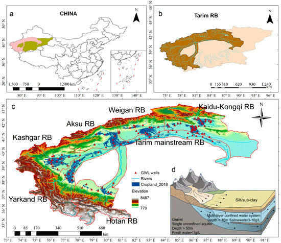
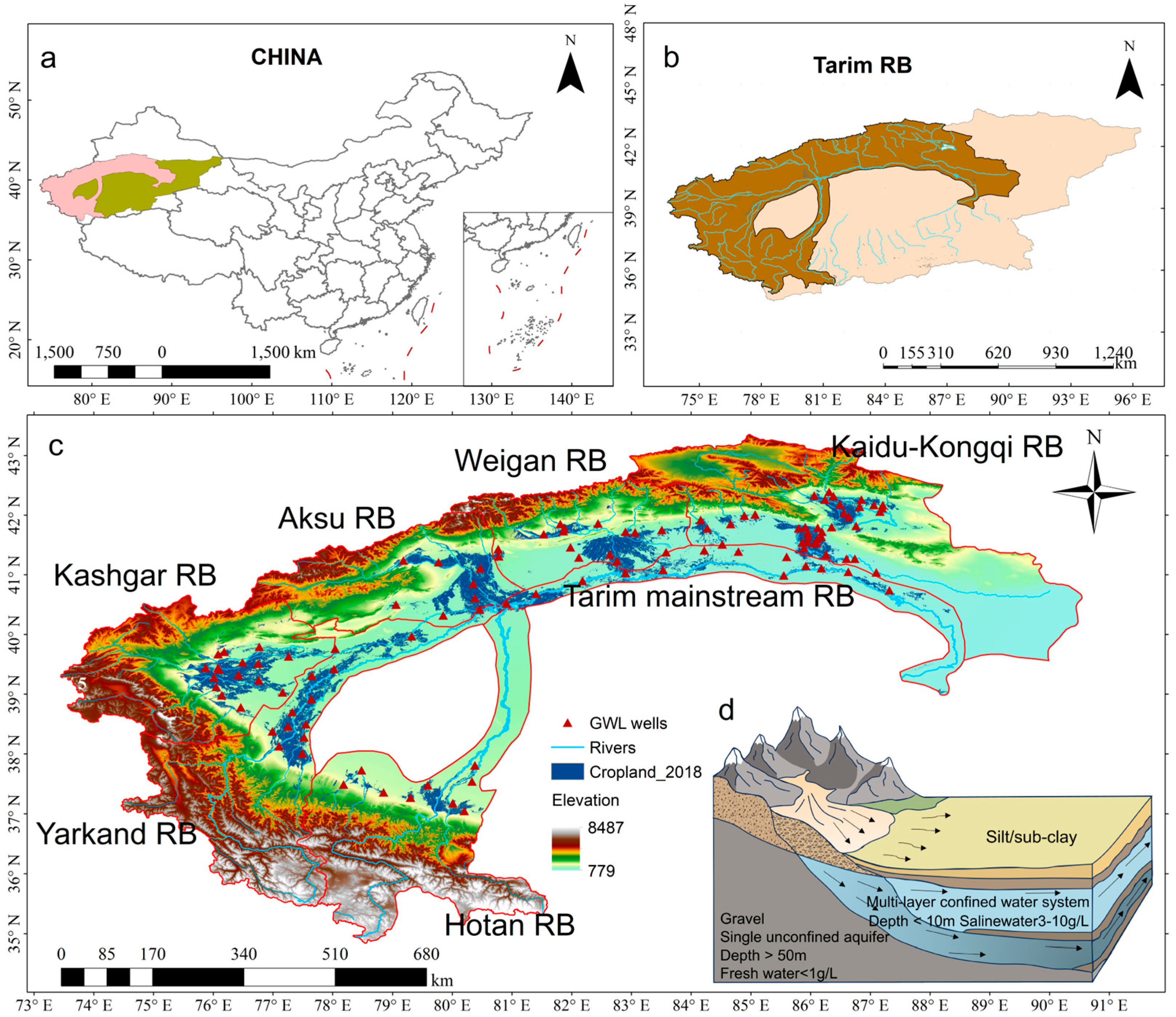
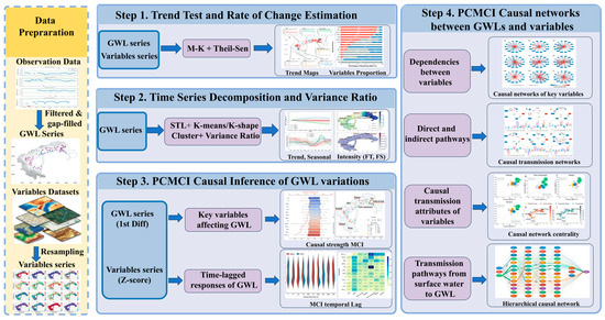
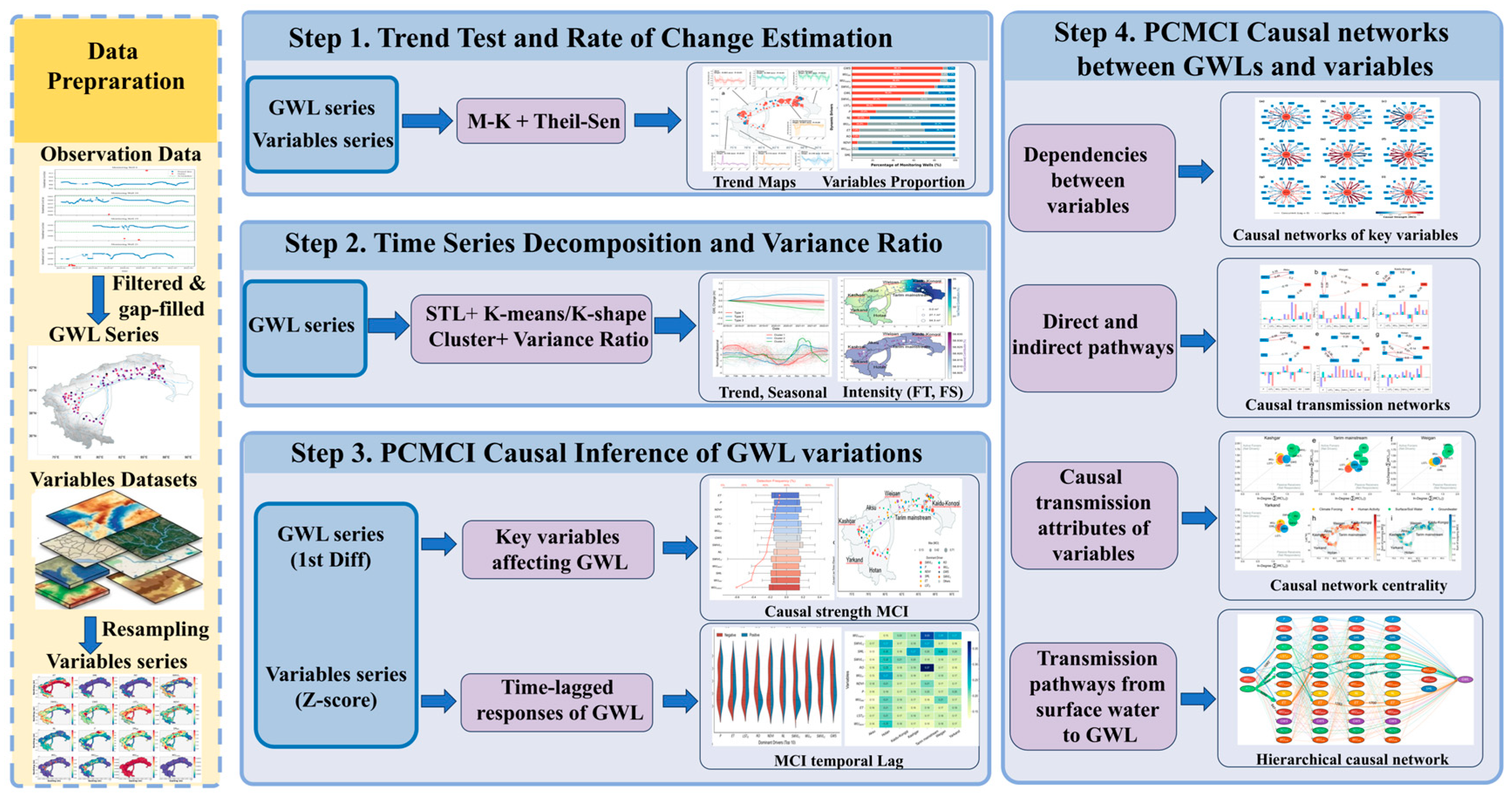
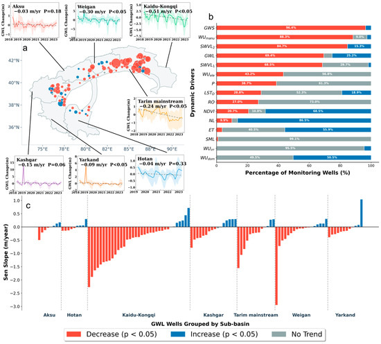
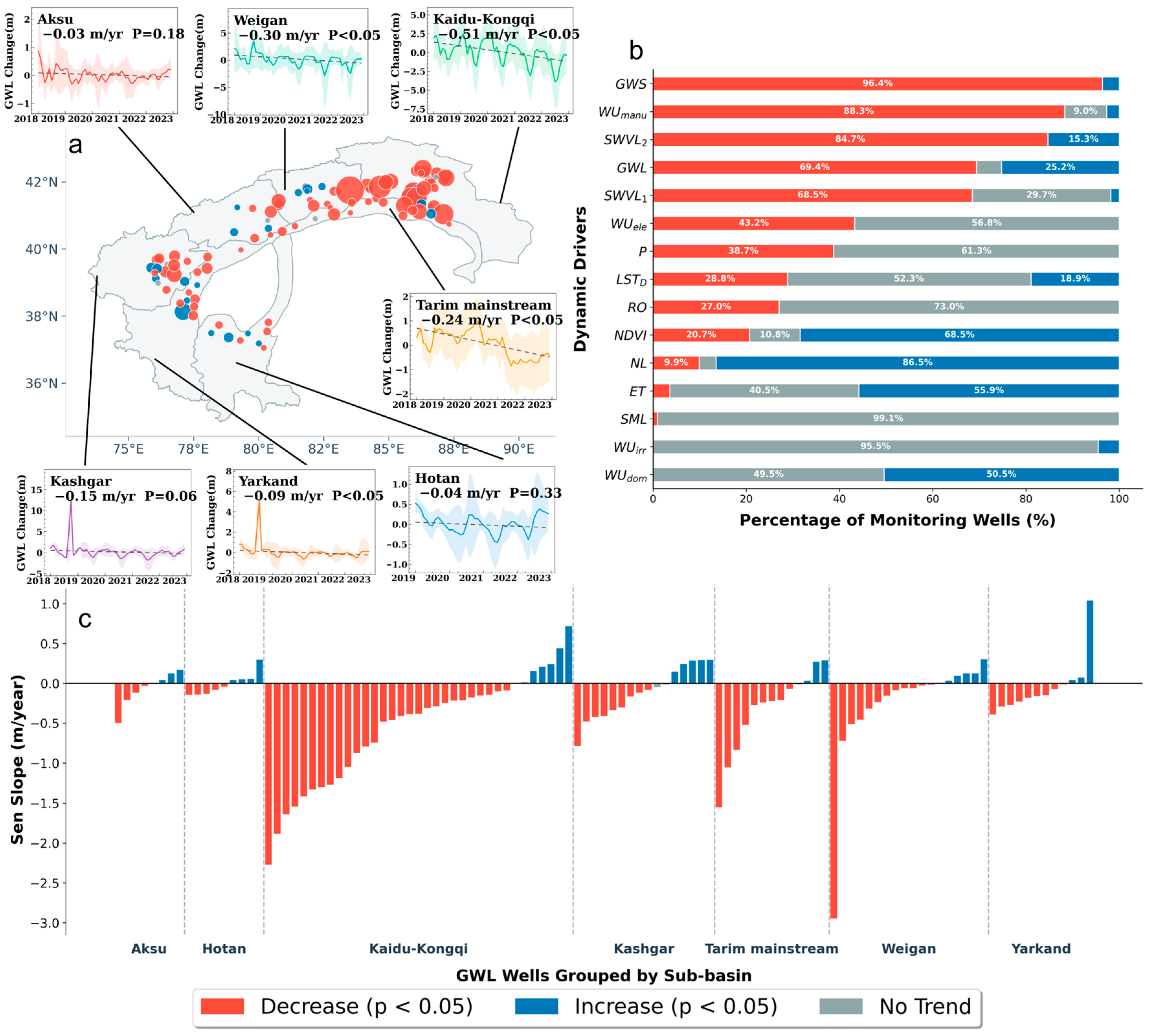
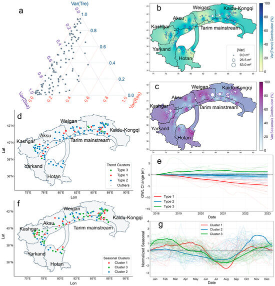
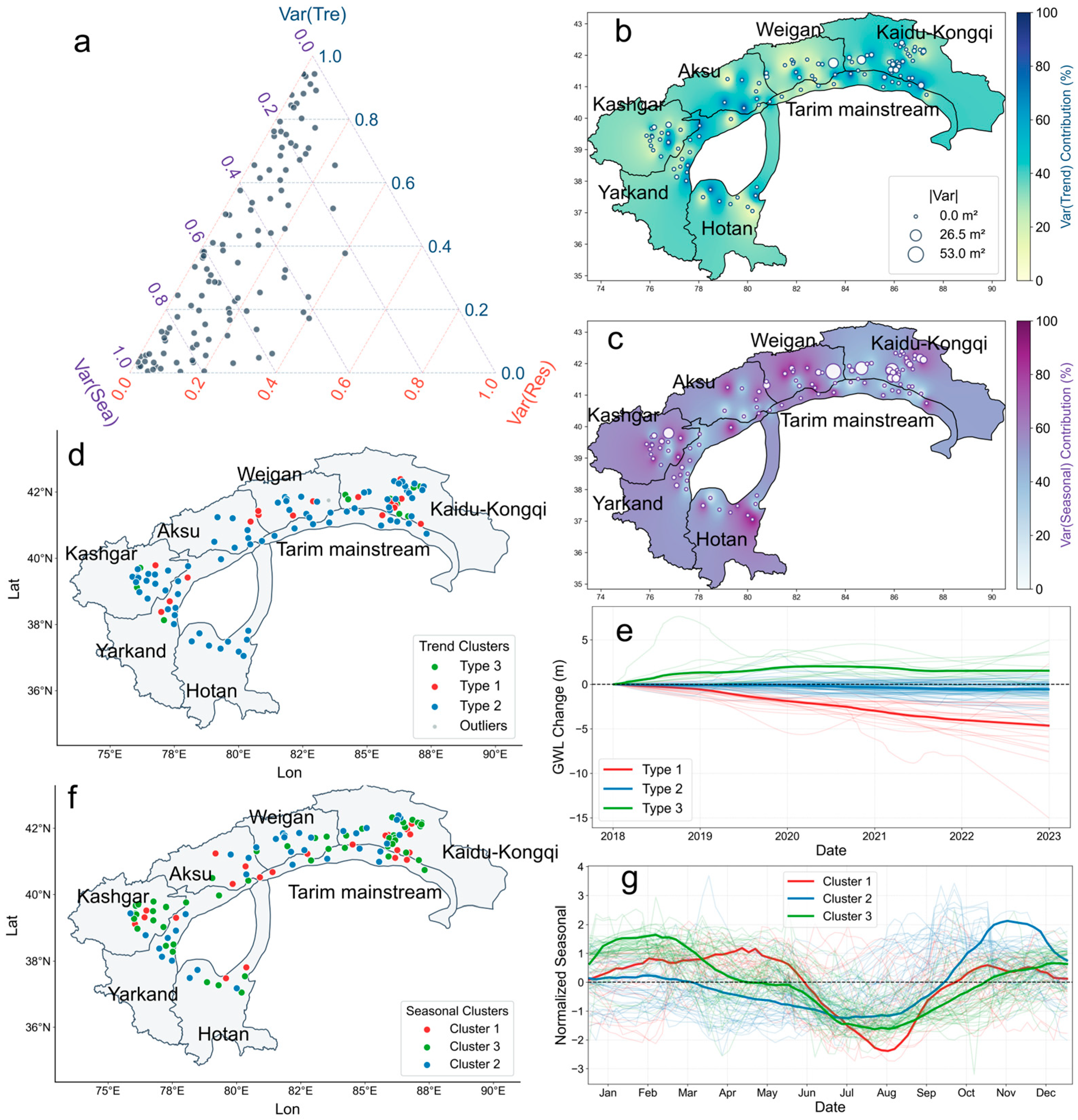
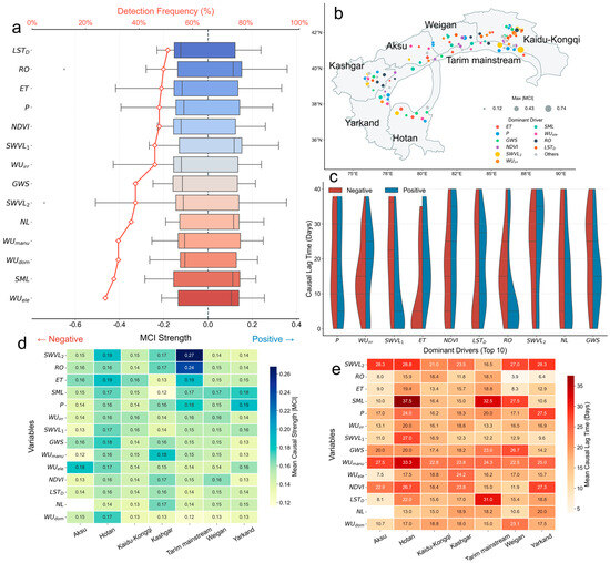
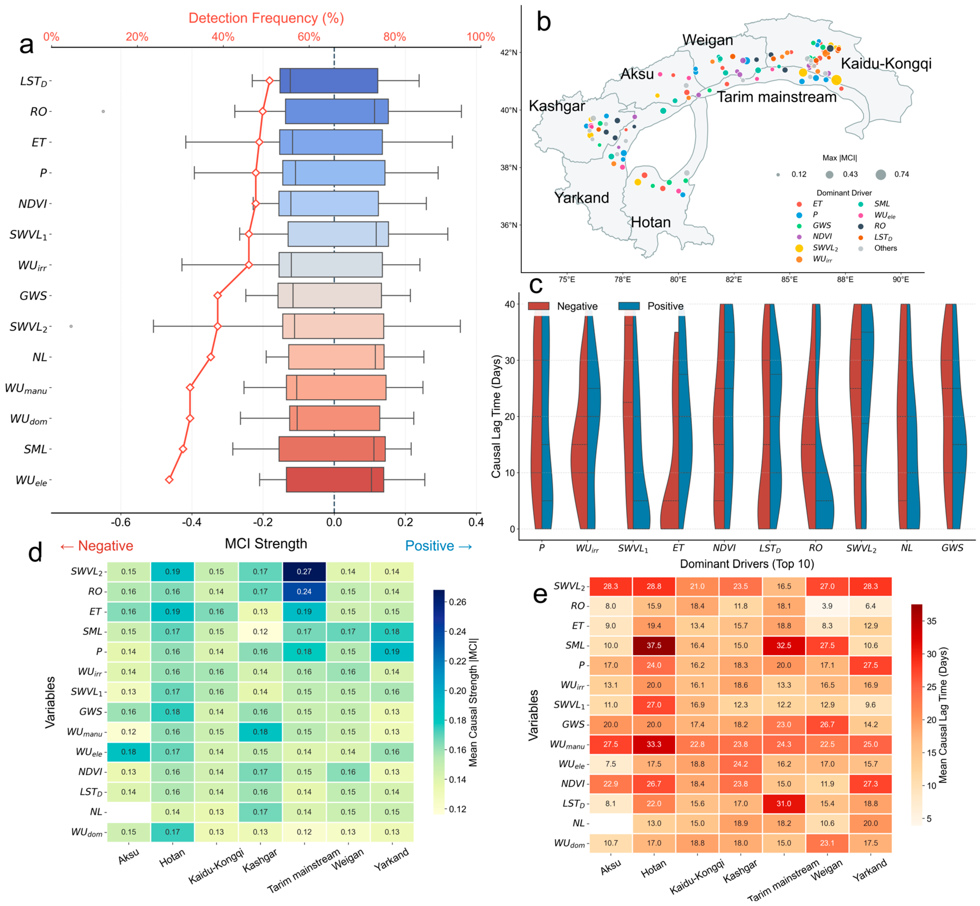
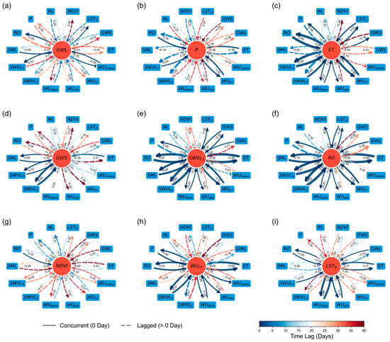
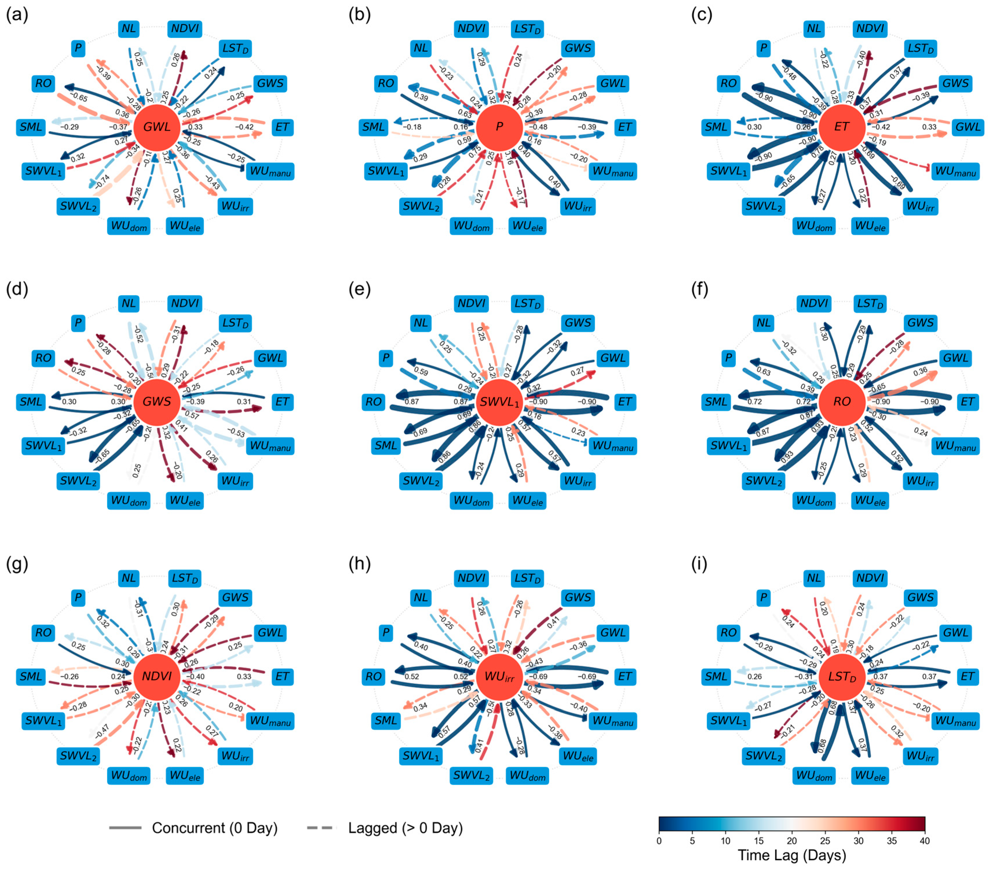
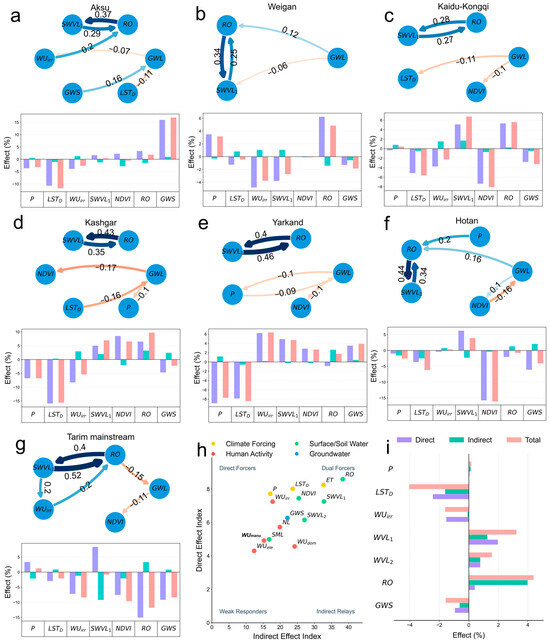
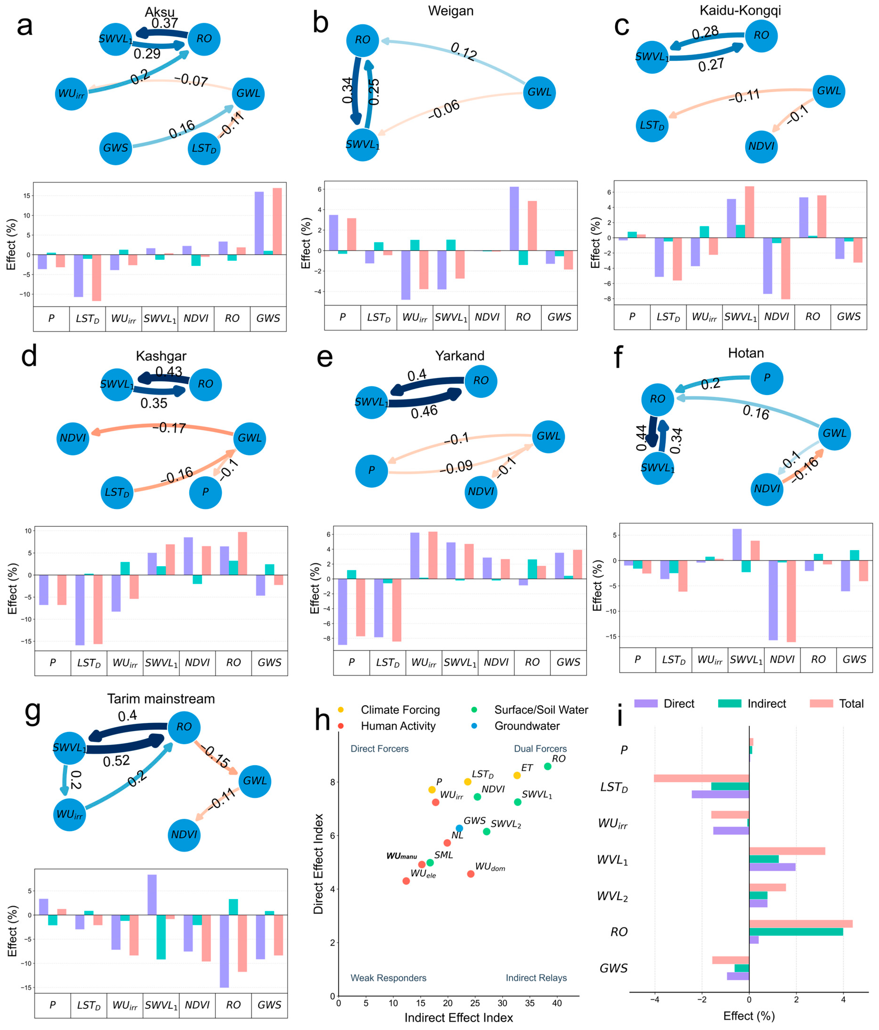
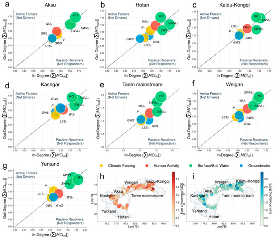
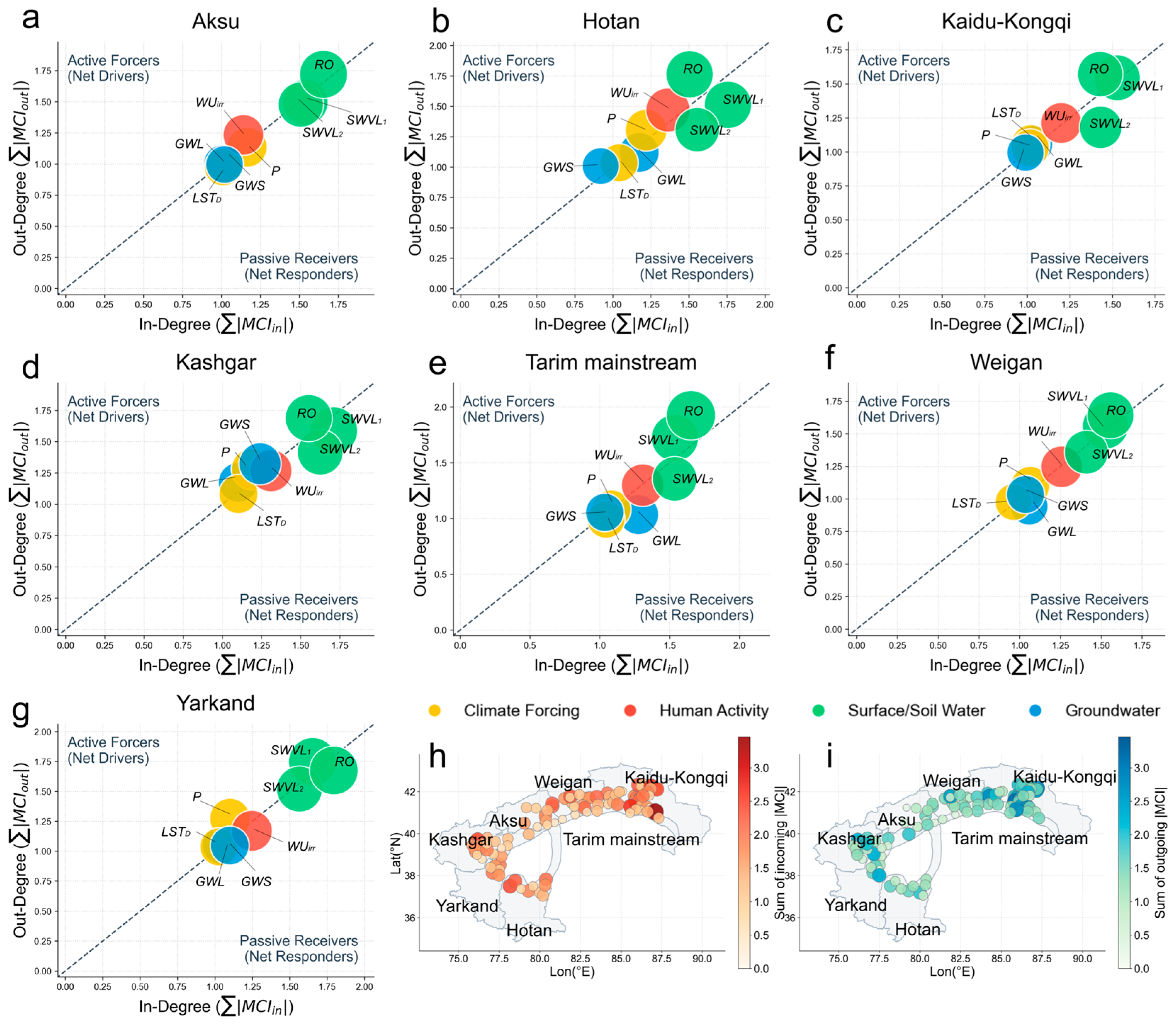
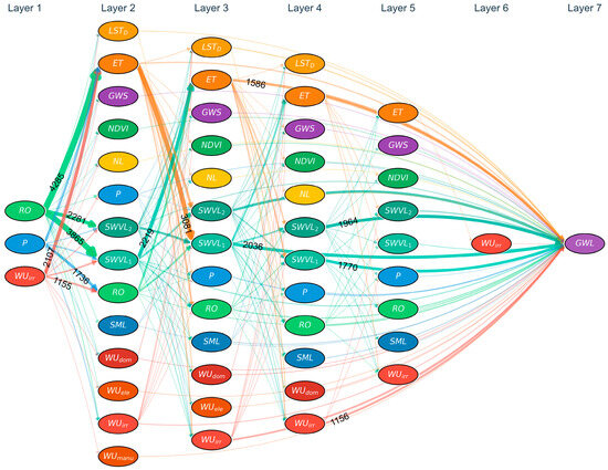
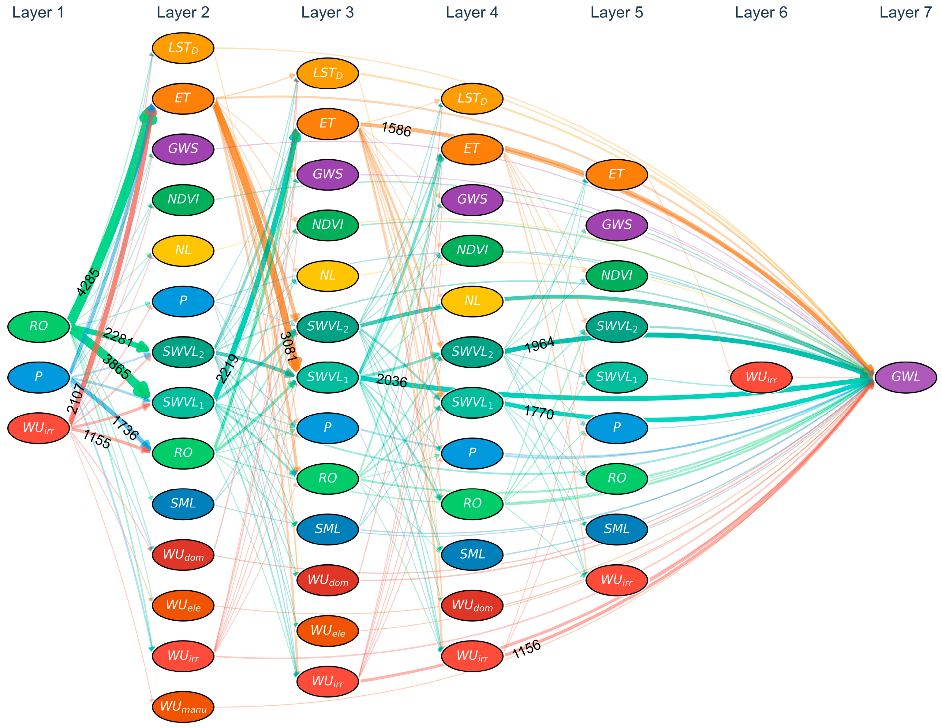
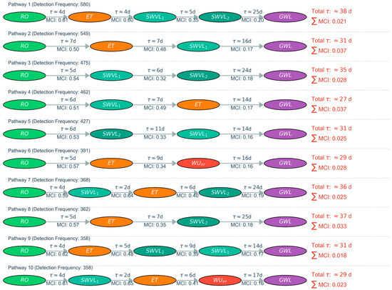
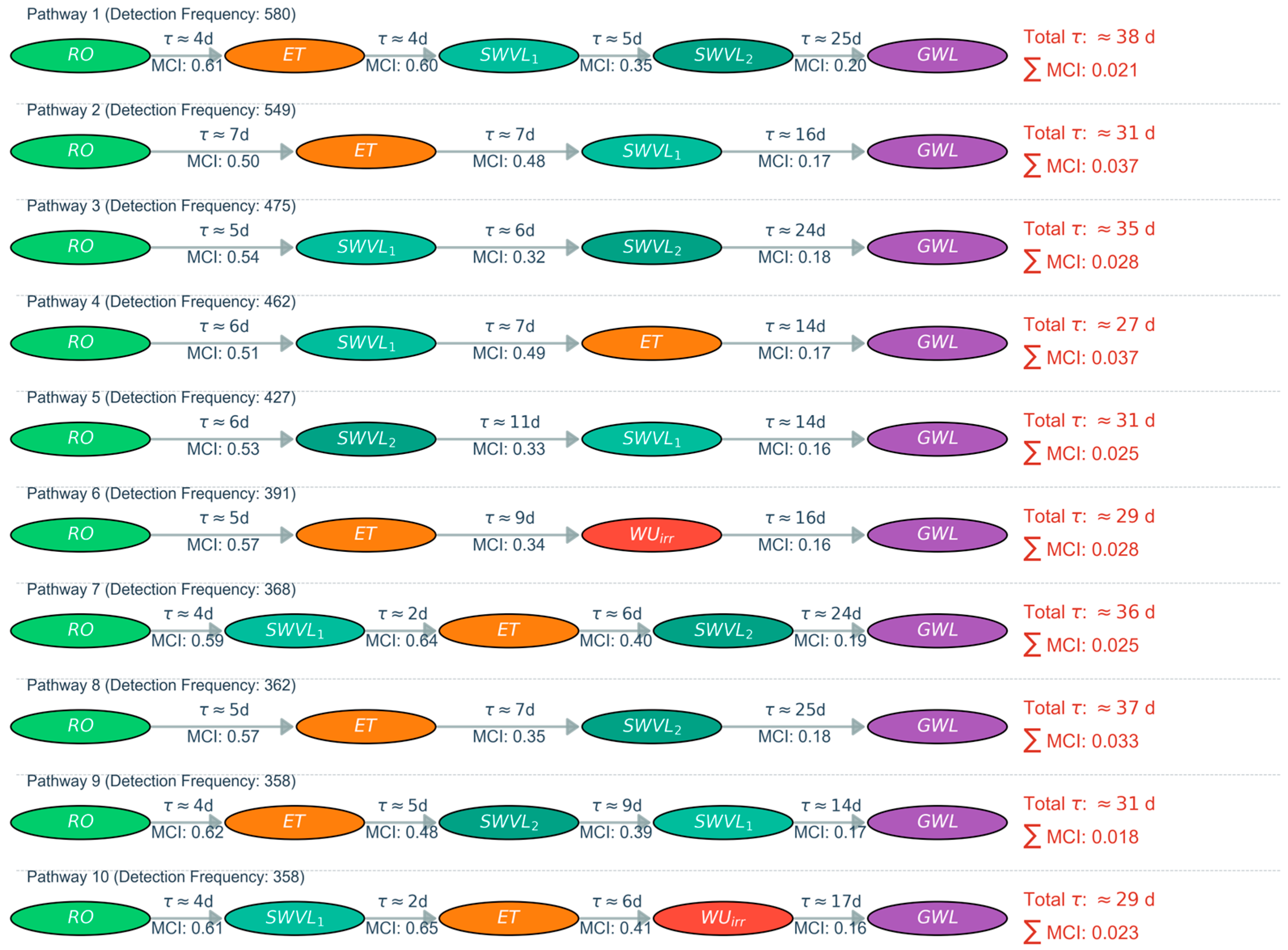
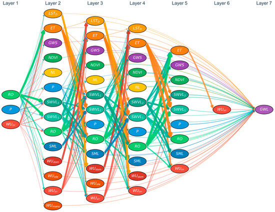
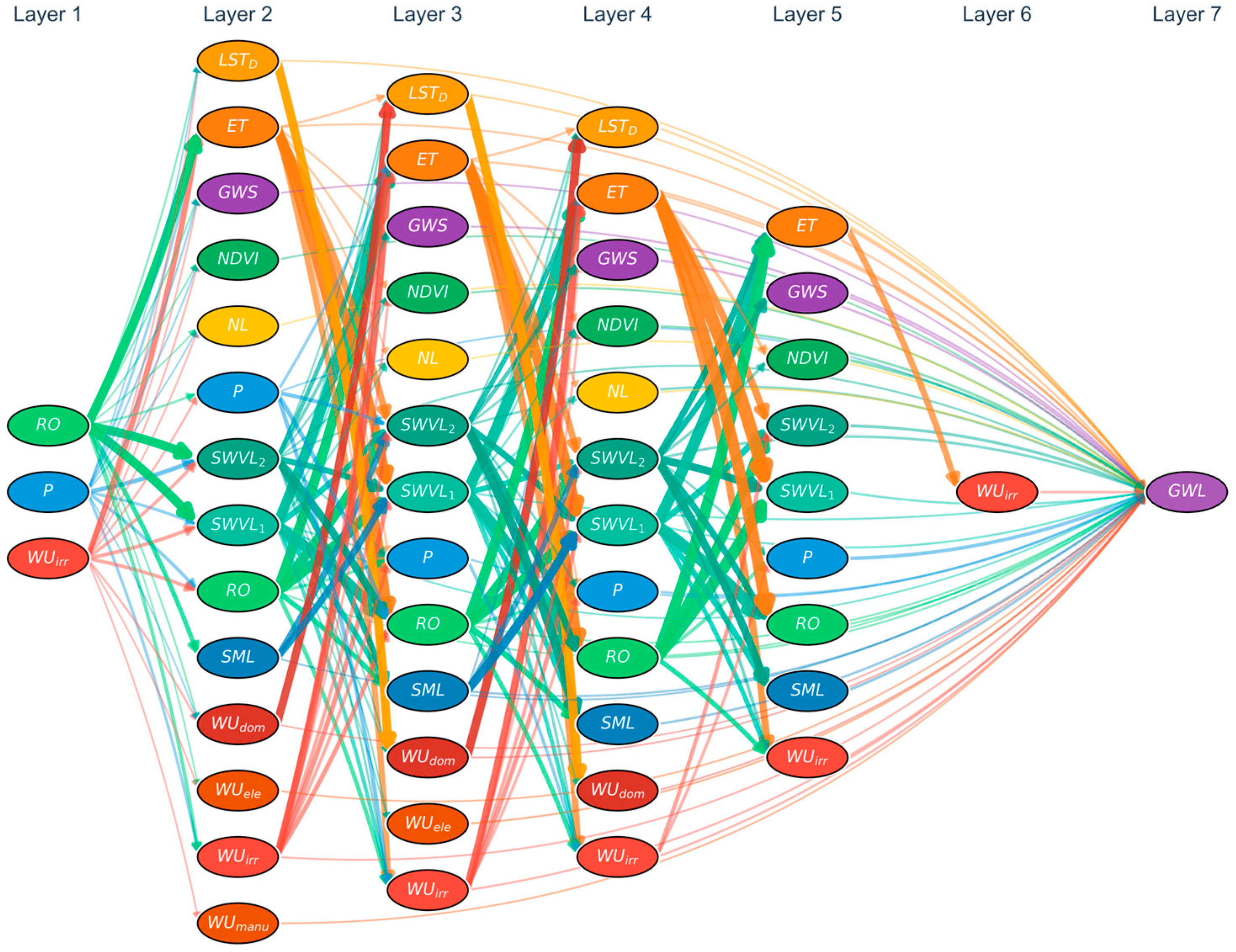
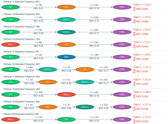
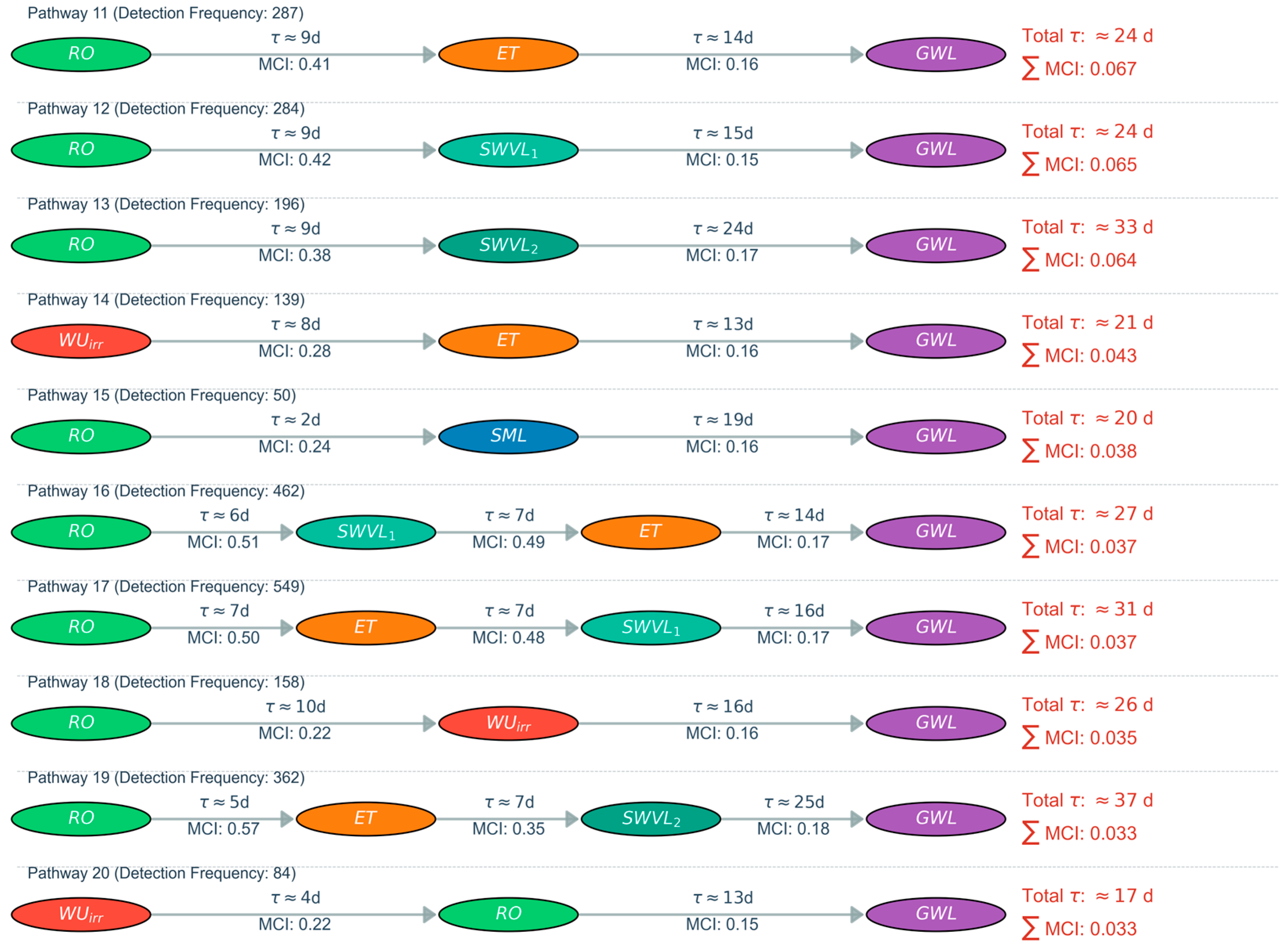

Disclaimer/Publisher’s Note: The statements, opinions and data contained in all publications are solely those of the individual author(s) and contributor(s) and not of MDPI and/or the editor(s). MDPI and/or the editor(s) disclaim responsibility for any injury to people or property resulting from any ideas, methods, instructions or products referred to in the content. |
© 2026 by the authors. Licensee MDPI, Basel, Switzerland. This article is an open access article distributed under the terms and conditions of the Creative Commons Attribution (CC BY) license.