Deep Learning Insights into Seamless Reconstruction of XCO₂ in China: Spatiotemporal Patterns and Driving Mechanisms

Highlights

What are the main findings?

• The Air-Transformer reconstructed a seamless daily 0.1° XCO₂ dataset over China for 2015–2020 with high accuracy (R² = 0.98, RMSE = 0.68 ppm).
• The reconstructed XCO₂ exhibits a significant upward trend of 2.68 ppm yr⁻¹ nationally, showing clear east-high/west-low and spring-high/summer-low patterns, with DEW, EM, and SP identified as the dominant drivers.

What are the implications of the main findings?

• This deep learning framework effectively overcomes the spatiotemporal limitations of current satellite observations and offers a reliable methodology for continuous greenhouse gas monitoring.
• Interpretable SHAP analysis uncovers the regional heterogeneity of XCO₂ drivers, providing a scientific basis for formulating differentiated carbon reduction policies.

Abstract

Accurate quantification of atmospheric column-averaged dry-air CO₂ mole fractions (XCO₂) is pivotal for quantifying carbon sources and supporting China’s dual carbon goals. However, existing satellite observations are limited by spatiotemporal gaps due to orbital constraints and atmospheric conditions. To bridge these gaps, we utilized a deep learning framework featuring a dual self-attention mechanism, Air-Transformer, to capture complex long-range spatiotemporal dependencies and non-linear interactions among variables. Utilizing OCO-2 retrievals and multi-source data, this approach generated a spatiotemporally consistent, daily 0.1° XCO₂ dataset over China during 2015–2020. Cross-validation demonstrates superior accuracy (R² = 0.98), with robust performance confirmed by spatial and temporal validation and ground-based TCCON benchmarks. The estimated full-coverage outputs reveal a national mean annual increase of 2.68 ppm, characterized by a distinct east-high/west-low pattern. Interpretable analysis based on Shapley Additive Explanations (SHAP) elucidates the non-linear interactions between XCO₂ and environmental drivers and exhibits significant regional heterogeneity. This spatiotemporally consistent and interpretable XCO₂ dataset offers vital data support for regional carbon monitoring and differentiated policy-making.

1. Introduction

Carbon dioxide (CO₂) is a primary driver of anthropogenic climate forcing, exerting profound impacts on the global climate system [1,2]. Driven by rapid urbanization and population growth, global atmospheric CO₂ concentrations surged from a pre-industrial level of ~280 ppm to 426.40 ppm as of March 2025 [3], a trajectory that acts as a critical trigger for global warming and the intensification of extreme weather events [4,5]. In 2024, China contributed 12.6 Gt of CO₂, accounting for approximately one-third of the global total [6]. Given this magnitude, China’s emission reduction trajectory plays a decisive role in curbing global climate change [7,8]. To address this, the nation has adopted ambitious dual carbon targets: peaking emissions before 2030 and achieving carbon neutrality by 2060 [9,10]. Therefore, generating high-resolution CO₂ data and gaining insights into the driving factors of concentration variations are of critical significance for the effective implementation of these policies.

Contemporary CO₂ monitoring relies primarily on ground-based networks, airborne platforms, and satellite remote sensing. While ground and airborne observations provide high accuracy, their spatial coverage is limited, and operational costs remain high [11]. In contrast, satellite missions such as GOSAT and OCO-2 offer large-scale observations of column-averaged dry-air CO₂ mole fractions (XCO₂) [12,13,14,15]. Notably, OCO-2 achieves high precision (<1 ppm), with fine spatial resolution (2.25 km × 1.29 km) [16]. However, due to orbital sampling constraints and interference from clouds and aerosols, satellite observations are inherently spatially discontinuous, limiting their direct application in continuous regional monitoring [17]. Although recent studies have applied machine learning methods for rapid XCO₂ retrieval, these approaches do not fundamentally resolve data fragmentation caused by observational limitations [18,19,20]. As a result, research has increasingly shifted toward data reconstruction to generate spatiotemporally continuous XCO₂ datasets.

In this context, data-driven machine learning methods have demonstrated clear advantages over traditional geostatistical interpolation and data assimilation in terms of reconstruction efficiency and accuracy [21,22]. Tree-based models, such as LightGBM and Extremely Randomized Trees, have been widely used to produce daily, full-coverage XCO₂ products over China [17,23]. Meanwhile, deep learning architectures, including spatiotemporal ResNet, ConvLSTM, and STAXN, have further improved the ability to represent complex spatial and temporal patterns, extending XCO₂ reconstruction to a 1 km resolution [24,25,26]. Nevertheless, existing approaches still face notable limitations. Tree-based models rely heavily on manually engineered features and struggle to capture high-dimensional spatiotemporal interactions. CNN- and LSTM-based models are effective in modeling local spatial structures or temporal dependencies, respectively, but remain limited in their ability to jointly capture long-range spatial correlations and long-term temporal dynamics. For atmospheric CO₂, which exhibits strong spatiotemporal autocorrelation and cross-scale transport processes, these limitations hinder the modeling of spatiotemporal consistency [27]. In contrast, transformer-based models leverage global self-attention mechanisms to directly learn long-range dependencies, making them well suited to characterize the complex spatiotemporal evolution of XCO₂ [28,29]. Therefore, introducing such architectures into XCO₂ reconstruction has the potential to improve both reconstruction accuracy and spatiotemporal consistency.

Beyond reconstruction accuracy, understanding the driving mechanisms of XCO₂ variability is also critical. The SHapley Additive exPlanations (SHAP) framework has been widely applied in atmospheric and air quality studies due to its ability to provide both global consistency and local interpretability. Previous studies have used SHAP to investigate the drivers of ozone pollution and PM_2.5 variability, revealing the contributions of meteorological and anthropogenic factors [30,31,32]. However, compared to evaluations of predictive performance, the systematic quantification of the relative contributions, interactions, and regional heterogeneity of multi-source drivers within non-linear models remains limited.

To address these challenges, this study adopts an adapted Air-Transformer framework with dual self-attention mechanisms to capture long-range spatiotemporal dependencies and non-linear interactions among multi-source variables. Using OCO-2 observations and auxiliary datasets, we reconstruct a seamless daily XCO₂ dataset over China at 0.1° resolution for the period 2015–2020. Based on this dataset, we analyze the spatiotemporal patterns of XCO₂ and further quantify the contributions and regional heterogeneity of key driving factors using SHAP. The results provide a robust data and methodological basis for carbon monitoring and region-specific mitigation strategies.

2. Materials and Methods

2.1. Study Area

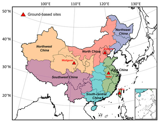
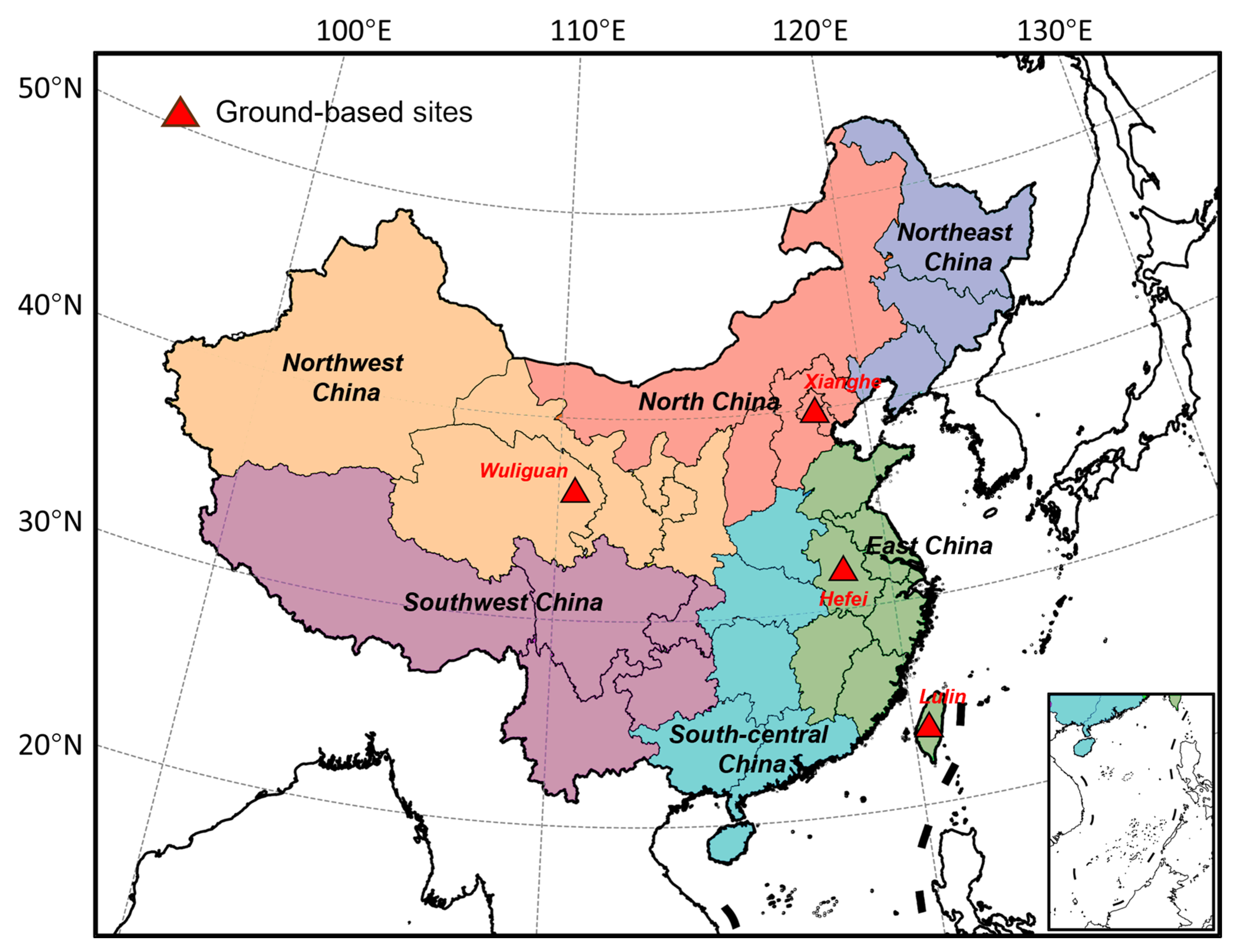
The study area covers the entirety of China (3°52′N–53°33′N, 73°40′E–135°05′E). To investigate XCO₂ spatial heterogeneity, the country was partitioned into six regions based on geographical and socio-economic characteristics (Figure 1): Northeast (NE), North (NC), East (EC), South Central (SC), Northwest (NW), and Southwest (SW) China. Seasons were defined as spring (March–May), summer (June–August), autumn (September–November), and winter (December–February).

Figure 1. Study area with six geographic subregions and distribution of ground-based validation sites.

2.2. Data Processing

This study utilized the OCO-2 Level 2 XCO₂ Version 11r product (L2_Lite_FP V11r) from January 2015 to December 2020, obtained from NASA GES DISC (https://disc.gsfc.nasa.gov/, last accessed on 2 March 2025). Strict quality control was applied using quality flags (xco2_quality_flag = 0) and an uncertainty threshold (xco2_uncertainty < 1.5 ppm). The filtered dataset comprises 291,899 validated pixels over China within the 0.1° grid, with mean daily spatial coverage of 0.14%, corresponding to approximately 133 valid pixels per day.

Meteorological data were sourced from the ERA5-Land reanalysis, including 2 m temperature (T2M), 2 m dewpoint temperature (DEW), a 10 m u-component (U10) and a v-component (V10) of wind, total precipitation (TP), boundary layer height (BLH), surface pressure (SP), and forecast albedo (ALB). Anthropogenic CO₂ emissions (EM) were obtained from the MEIC model [33]. To characterize surface processes, we incorporated the monthly Normalized Difference Vegetation Index (NDVI) data from MODIS [34], accumulated CO₂ gross primary production (GPP) from Copernicus Atmosphere Monitoring Service (CAMS), the annual population distribution (POP) from WorldPop, elevation (ELV) from ASTER Global Digital Elevation Model data, and land-use classification products (LU) sourced from the Resource and Environmental Science Data Platform.

To address satellite data gaps, we utilized the CAMS global CO₂ reanalysis, which provides 0.75° × 0.75° spatial resolution with 3-hourly temporal resolution [35]. Despite its coarse resolution, it delivers physically consistent constraints for regional modeling applications [36,37]. This study established a 0.1° × 0.1° daily gridded dataset aligned with study area boundaries. All auxiliary datasets were systematically resampled to the target resolution and matched with OCO-2 XCO₂ retrievals. Specifically, for datasets with a spatial resolution finer than the target grid, the area-weighted averaging resampling method was applied; for datasets with coarser resolution, bilinear interpolation was employed to ensure spatial consistency; and for discrete categorical data (e.g., land use), majority resampling was utilized to preserve the integrity of categorical boundaries. Following spatiotemporal gridding, all variables were normalized using the Z-score standardization method to eliminate scale effects. The Z-score is defined as:

$$z={\displaystyle \frac{x-\mu }{\sigma }}$$

(1)

where x represents the original value, μ is the mean of the variable, and σ denotes the standard deviation.

The final dataset was structured as multi-dimensional arrays, where variables were organized as daily spatial grids of size 700 × 500, serving as standardized inputs for subsequent model training. All the datasets and their corresponding details are presented in Table 1.

Table 1. Summary of multiple data sources.

Category	Variable Name	Source	Resolution	Scale	Unit
Emission	CO2 emissions	http://meicmodel.org.cn/	0.1° × 0.1°	Monthly	Mg
Meteorology	10m u-component of wind	https://cds.climate.copernicus.eu/	9 km	Hourly	m/s
	10m v-component of wind				m/s
	Total precipitation				m
	2 m temperature				K
	2 m dewpoint temperature				K
	Boundary layer height				m
	Surface pressure				Pa
	Forecast albedo				(0–1)
Surface Data	NDVI	MODIS	1 km	Monthly	(0–1)
	Population	WorldPOP		Annual	/km2
	Elevation	https://www.resdc.cn/		Constant	m
	Land use			Constant	-
CAMS Data	Accumulated CO2 gross primary production	https://ads.atmosphere.copernicus.eu/	0.75° × 0.75°	3-hourly	kg/m2
	CO2 column-mean molar fraction				ppm
Time	Day of year	-	-	Daily	-
Label	OCO-2	https://disc.gsfc.nasa.gov/	2.25 km × 1.29 km	Daily	ppm

2.3. Deep Learning Model Architecture

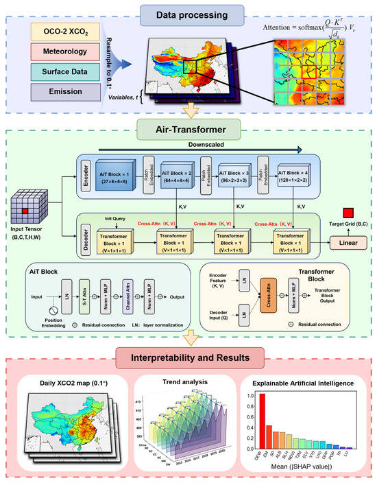
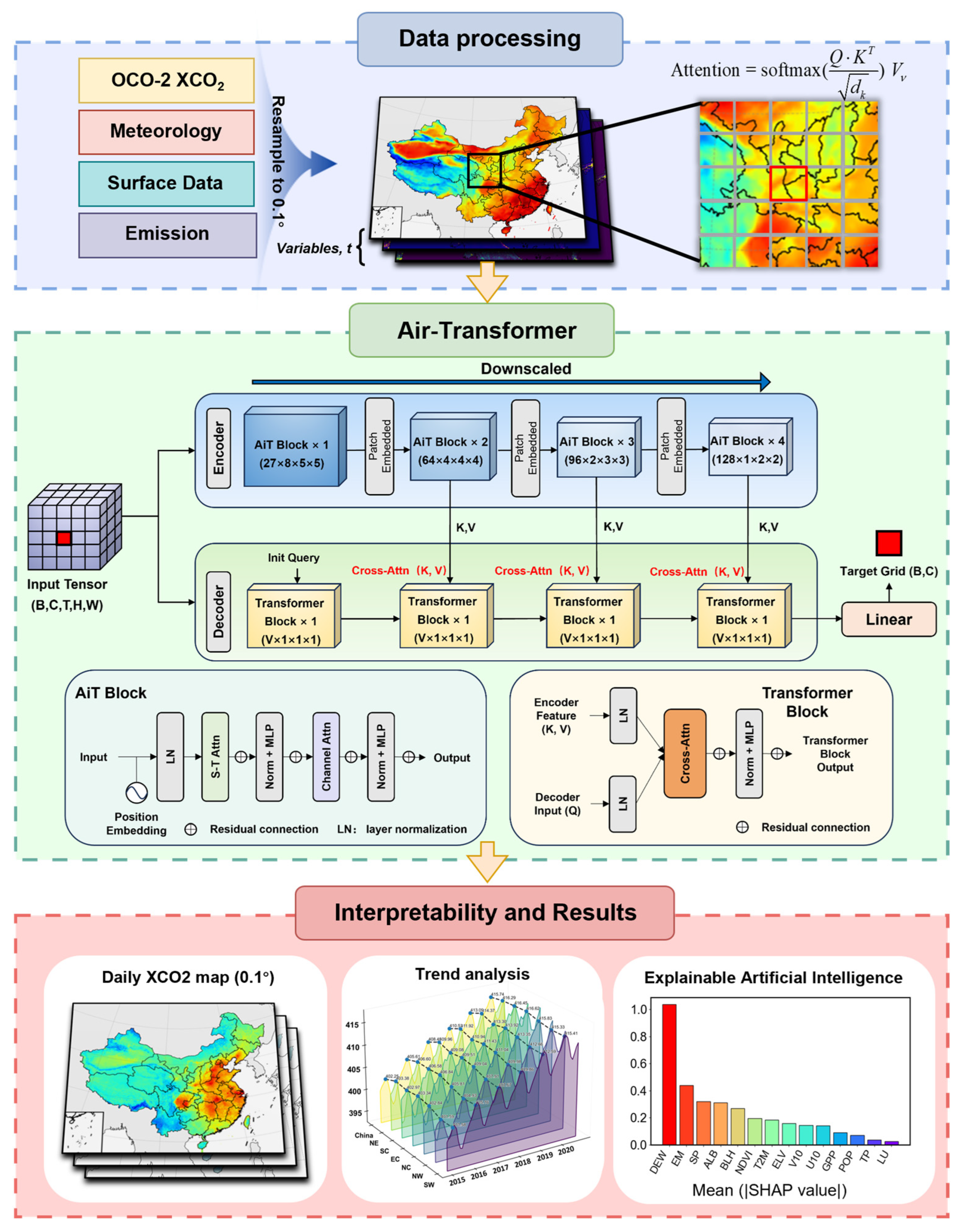
The Air-Transformer employed in this study is a transformer-based deep learning framework for atmospheric science applications, which has previously been applied in ozone concentration studies [38,39]. As shown in Figure 2, the model adopts an encoder–decoder architecture with an innovative dual self-attention mechanism to learn complex spatiotemporal relationships in XCO₂ from gridded sequential data and multi-source environmental auxiliary variables, thereby enabling high-accuracy reconstruction of XCO₂ concentrations. The input tensor dimensions are defined by the number of variables (V) and the spatiotemporal window size. In this study, we selected 27 input variables (V = 27) including 15 feature variables and 12 spatiotemporal variables. For these 12 spatiotemporal variables, we constructed a 12-component spatiotemporal feature vector framework to better characterize the spatiotemporal correlations embedded in the raw latitude, longitude, and temporal information while mitigating boundary discontinuities. The spatial components include longitude, latitude, and Euclidean spherical coordinates (Equations (2)–(4)), whereas the temporal components include Julian day, year, and cyclical trigonometric encodings of day of week, month, and season (Equations (5)–(7)). The temporal window size was set to 8 frames, and the spatial window size was set to 5 × 5 grids. Consequently, the input data shape is initialized as 27 × 8 × 5 × 5.

$$s_1=\cos (2\pi {\displaystyle \frac{longitude}{360}})\cos (2\pi {\displaystyle \frac{latitude}{180}})$$

(2)

$$s_2=\cos (2\pi {\displaystyle \frac{longitude}{360}})\sin (2\pi {\displaystyle \frac{latitude}{180}})$$

(3)

$$s_3=\sin (2\pi {\displaystyle \frac{longitude}{360}})$$

(4)

$${\cos }_{sea}=\cos (2\pi {\displaystyle \frac{month}{12}})$$

(5)

$${\sin }_{sea}=\sin (2\pi {\displaystyle \frac{month}{12}})$$

(6)

$${\cos }_{month}={\displaystyle \frac{month}{360}}$$

(7)

Figure 2. Schematic workflow of the Air-Transformer model.

The Air-Transformer encoder is structured into four hierarchical stages with block depths of {1, 3, 2, 1}. The first stage maintains the original input resolution. In the subsequent three stages, we employ convolutional embedding blocks for down-sampling, utilizing a 2 × 2 × 2 kernel with a stride of 2 × 2 × 1. This design progressively maps the hidden layer dimensions from the initial 27 to {64, 96, 128}, yielding feature maps of sizes 64 × 4 × 5 × 5, 96 × 2 × 5 × 5, and 128 × 1 × 5 × 5, respectively, thereby capturing the distribution characteristics of XCO₂ across different spatiotemporal scales. Within these blocks, the encoder maps the input sequence of neighborhood spatiotemporal data into a sequence with high-dimensional spatiotemporal features, while the decoder generates representation estimates by computing the attention between the target grid and the encoder output. Specifically, global spatiotemporal self-attention is applied over pixel sequences (N = H × W) to extract regional XCO₂ patterns. In parallel, channel-wise self-attention functions over variable sequences to uncover latent relationships between environmental factors and XCO₂ (Equation (8)).

$$\mathrm{Attention} (Q,K,V)=\mathrm{softmax}({\displaystyle \frac{Q{K}^T}{\sqrt{d_k}}}+B) V$$

(8)

where Q, K, V denote the query, key, and value matrices of the input sequence, respectively, d_k is the key dimension, and B is a geographic positional bias term designed to correct systematic latitude–longitude-dependent errors.

The model was trained using the AdamW optimizer, incorporating a warm-up strategy for the initial 30 epochs to ensure optimization stability. The Mean Squared Error (MSE) was adopted as the loss function (Equation (9)). Throughout the network, the Gaussian Error Linear Unit (GeLU) was utilized as the activation function. We selected a batch size of 128, a configuration designed to balance GPU memory consumption with training efficiency while ensuring gradient stability. To further mitigate overfitting, a dropout rate of 0.05 was applied to all linear and self-attention layers, and early stopping was triggered if the validation loss did not improve for 50 consecutive epochs.

$$\mathrm{MSE}={\displaystyle \frac{1}{n}}{\displaystyle \sum _{i=1}^n{(y_i-{\widehat{y}}_i)}^2}$$

(9)

where ${\widehat{y}}_i$ and $y_i$ are the predicted and observed values for the i-th sample, respectively, and n is the total number of samples.

2.4. Validation Methods

To rigorously assess model generalization and stability, a multi-dimensional cross-validation (CV) framework was implemented, comprising three distinct schemes. First, a sample-based 10-fold CV was conducted by randomly partitioning the dataset into ten subsets for iterative validation. Second, to evaluate temporal extrapolation ability, a temporal 10-fold CV was performed by chronologically splitting the dataset from 2015 to 2020 into ten consecutive time segments, with one subset reserved for testing in each fold and the remaining subsets used for training. Third, to assess spatial generalization, a spatial 10-fold CV was conducted by dividing the study domain into ten geographically distinct subregions (2 × 5 blocks), with one subregion excluded for validation in each fold. Model performance was quantified using the coefficient of determination (R²) and root mean square error (RMSE) (Text S1).

Independent validation employed high-precision ground-based XCO₂ measurements from the Total Carbon Column Observing Network (TCCON) [40]. Data were acquired from two stations: Hefei (31.9°N, 117.17°E; November 2015–December 2020) and Xianghe (39.8°N, 116.96°E; June 2018–December 2020). TCCON provides column-averaged XCO₂ measurements and is widely used as a reliable reference for validating satellite-derived and reconstructed XCO₂ products [41,42]. To further strengthen the evaluation, we additionally included two supplementary surface sites from the World Data Centre for Greenhouse Gases (WDCGG), Mt. Waliguan (WLG; 36.28°N, 100.90°E), and Lulin (LLN; 23.47°N, 120.87°E). It should be noted that WLG and LLN provide near-surface CO₂ measurements rather than column-averaged XCO₂. Therefore, these two sites were used as auxiliary reference data to assess the temporal consistency of the reconstructed product, rather than as fully equivalent independent validation targets for XCO₂.

2.5. Analysis of XCO₂ Driving Factors

Interpretability analysis can provide insight into how environmental drivers are represented in a complex reconstruction framework and strengthen confidence in the reconstructed XCO₂ patterns. This study employed the SHAP framework to characterize the contributions of environmental variables to XCO₂ variability [43]. Given the computational intractability of SHAP attribution for high-dimensional spatiotemporal neural networks, we adopted a surrogate-based interpretability strategy [38]. Specifically, the continuous XCO₂ estimations generated by Air-Transformer during 2015–2020 served as target outputs, and the SHAP values were efficiently computed using a combination of the LightGBM model and the SHAP interpretability method, employing the GPUTreeShap algorithm [44]. The surrogate model exhibited good performance with the Air-Transformer estimations, supporting its use as a computationally efficient basis for analyzing the contribution of driving factors to XCO₂ variability (Figure S1). In addition, SHAP provides a unified measure that elucidates feature contributions at both the global dataset level and the individual sample level (Equations (10) and (11)).

$${\varphi }_{\mathrm{i}}={\varphi }_{base}+{\displaystyle \sum _{j=1}^{N}shap(x_{i,j})}$$

(10)

$$shap(x_{i,j})={\displaystyle \sum _{S\subseteq \{x_{i,1},x_{i,2},\dots ,x_{i,n}\}/\left\{x_{i,j}\right\}}\frac{\left|S\right|!(|N|-|S|-1)!}{\left|N\right|!}[\varphi (S\cup \{x_{i,j}\}-\varphi (S))]}$$

(11)

where ${\varphi }_{\mathrm{i}}$ is the predicted value generated for each sample i with N factors, ${\varphi }_{base}$ is the expected value of ${\varphi }_{\mathrm{i}}$, x_i,j denotes the factor j for sample i, and shap(x_i,j) is the Shapley value of the impact of the factor j on ${\varphi }_{\mathrm{i}}$ at sample i. S is a subset of factors used in the model, |S| is the number of non-zero entries in S. ${\varphi }_{(S)}$ is the predicted value of subset S. shap(x_i,j) > 0 indicates the positive effect of factor j that increases the prediction above the base value, and shap(x_i,j) < 0 indicates the opposite.

2.6. Trend Analysis Methods

To characterize the spatiotemporal evolution of XCO₂ based on the generated dataset, we employed the Seasonal-Trend decomposition using Loess (STL) and the Mann–Kendall trend test. First, the STL method was implemented to decouple the time series into deterministic components, owing to its robustness against outliers (Equation (12)).

$$y_t=T_t+{\displaystyle {\sum }_{i=1}^I{S}_t^{(i)}}+R_t$$

(12)

where T_t is the trend component, S_t⁽ⁱ⁾ is the i-th seasonal component, and R_t is the remaining component at time t. Subsequently, the nonparametric Mann–Kendall test was applied to quantify the significance of monotonic trends (Equation (13)).

$$S={\displaystyle {\sum }_{i=1}^{n-1}{\displaystyle {\sum }_{j=i+1}^n\mathrm{sgn}(y_j-y_i)}}$$

(13)

where n represents the sample size, and y denotes the data points at times j and i. A positive (negative) S value indicates a significant increasing (decreasing) trend in the XCO₂ concentrations, while a value near zero implies no significant trend.

3. Results and Discussion

3.1. Model Performance

3.1.1. Model Accuracy Evaluation

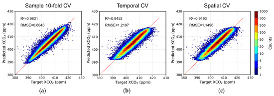
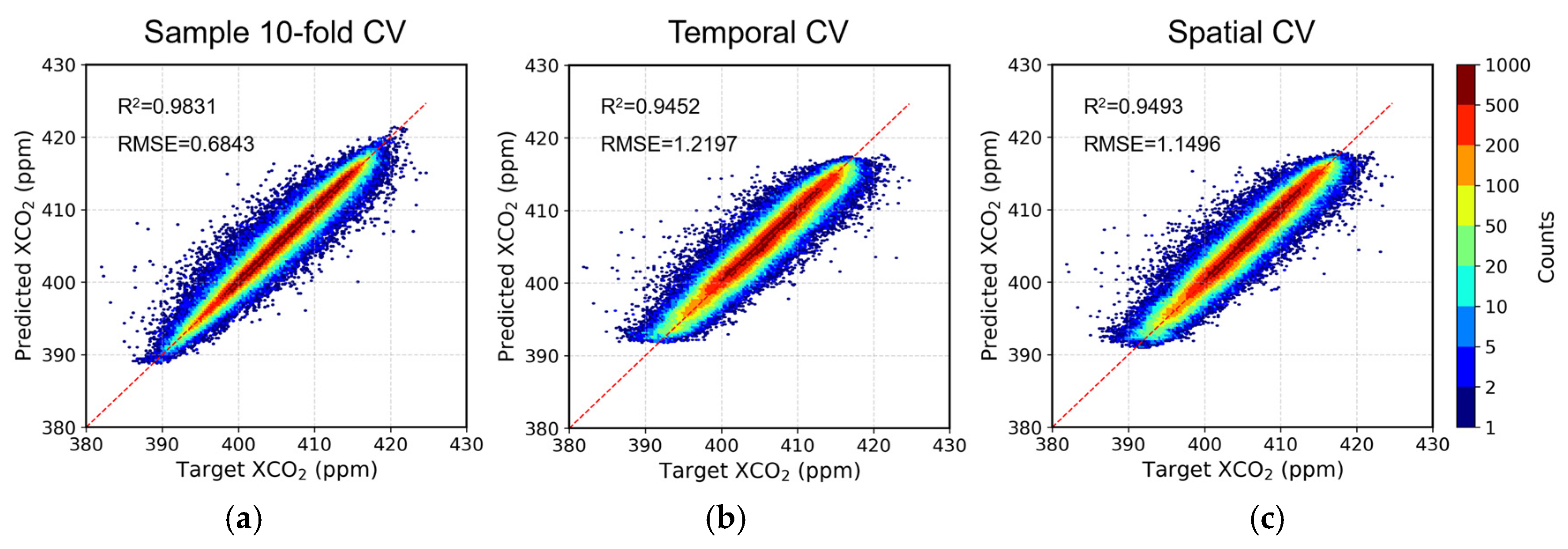
The predictive performance of the Air-Transformer was evaluated under three complementary cross-validation schemes, including random sample-based, temporal, and spatial 10-fold CV (Figure 3). The model demonstrated exceptional accuracy in the sample-based 10-fold CV, achieving an R² of 0.98 and RMSE of 0.68 ppm. Crucially, the model maintained robust performance in extrapolation tasks, showing only marginal degradation compared to random sampling. Specifically, under the strict temporal CV, the model yielded an R² of 0.95 and an RMSE of 1.22 ppm. Furthermore, in the spatial CV, the model achieved an R² of 0.95 and an RMSE of 1.15 ppm. Although the performance under temporal and spatial CV was lower than that under random CV, the decrease was moderate, indicating that the model retains strong predictive capability beyond local spatiotemporal similarity. In addition, seasonal spatial bias maps show that the spatial biases were generally within −1 to 1 ppm across the four seasons (Figure S2).

Figure 3. Evaluation of Air-Transformer performance for XCO₂ prediction. Scatterplots comparing daily OCO-2 observations and model predictions for (a) sample-based 10-fold CV, (b) temporal CV, and (c) spatial CV.

To objectively evaluate the structural advantages of the Air-Transformer, we conducted a standardized benchmark comparison against representative models (ResNet, Random Forest, and LightGBM) using the exact same dataset and validation protocols. As detailed in Table S1, Air-Transformer consistently outperformed all baseline models across all validation schemes. The performance gap was particularly pronounced in the spatial and temporal CVs, supporting its improved ability to capture complex spatiotemporal dependencies in XCO₂.

Prior studies indicated that model performance tends to decline significantly when CAMS data is excluded, suggesting a potential risk of over-reliance. Our sensitivity analysis reveals that Air-Transformer retains high robustness without CAMS, still maintaining a 10-fold cross-validation R² of 0.98 (Figure S3a). This proves the model captures spatiotemporal XCO₂ dynamics through dual attention mechanisms, rather than merely downscaling interpolation on coarse resolution CAMS data. Nevertheless, independent TCCON validation highlights the necessity of CAMS for absolute precision. Upon the exclusion of CAMS, R² against the Hefei TCCON site decreased from 0.90 to 0.85, and for the Xianghe site, it dropped from 0.81 to 0.74 (Figure S3b). The result indicates that while the model independently reconstructs distribution patterns, the physically consistent constraints and background concentration information provided by CAMS are crucial for correcting systematic biases.

3.1.2. Ground-Based Validation Results

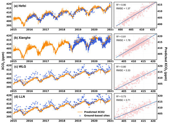
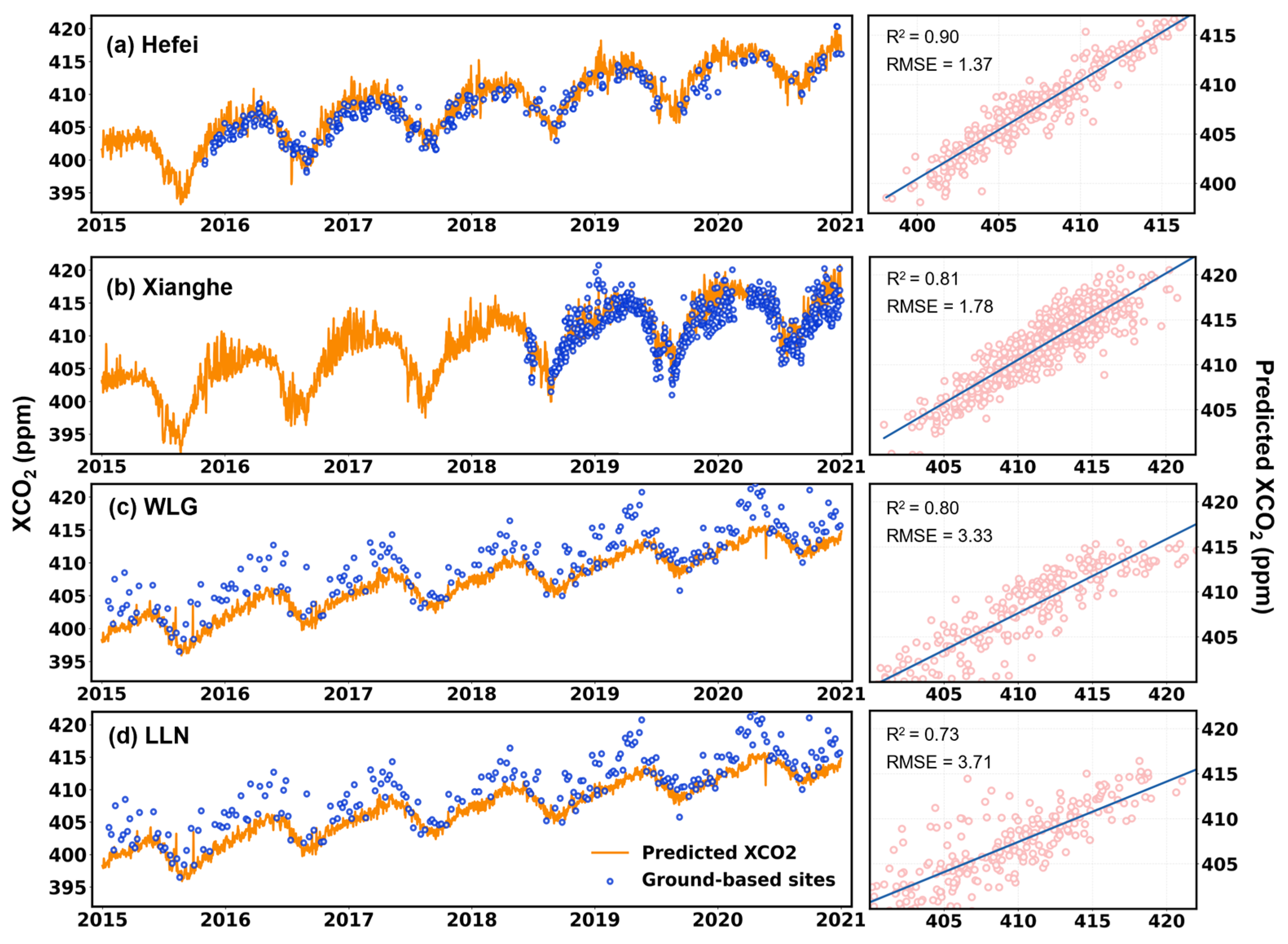
Independent validation against TCCON measurements further corroborates the model’s accuracy (Figure 4a,b). The model demonstrated high fidelity at the Hefei station (348 days), achieving an R² of 0.90. At the Xianghe station (592 days), while the model maintained a strong correlation (R² = 0.81), a systematic underestimation was observed for concentrations exceeding 415 ppm. This specific discrepancy is likely attributable to the greater environmental complexity and potential data quality constraints at the site [25]. Despite these localized variations, the overall consistency with ground-based observations substantiates the reliability of the Air-Transformer estimates.

Figure 4. Comparisons between reconstructed XCO₂ and ground-based observations.

To further supplement the validation, we compared the reconstructed XCO₂ with near-surface CO₂ observations from WLG and LLN stations (Figure 4c,d). The reconstructed results showed strong temporal consistency with these surface records, with R² values of 0.80 and 0.73 and RMSE values of 3.33 and 3.71 ppm for WLG and LLN, respectively. These results suggest that the reconstructed product is able to capture the major temporal variability of atmospheric CO₂, while the smaller amplitude of XCO₂ compared with near-surface CO₂ is physically expected due to its vertically integrated nature. Despite these additional comparisons, independent validation remains limited by the availability of long-term ground observations in some regions of China. This issue should be further improved as more observation sites become available in future studies.

3.1.3. Reconstruction Results

Using the Air-Transformer model, this study reconstructed a spatiotemporally continuous daily XCO₂ dataset over China at 0.1° × 0.1° resolution for the period 2015–2020. The dataset spans 2192 days and includes 96,166 valid grid cells per day within the national boundary.

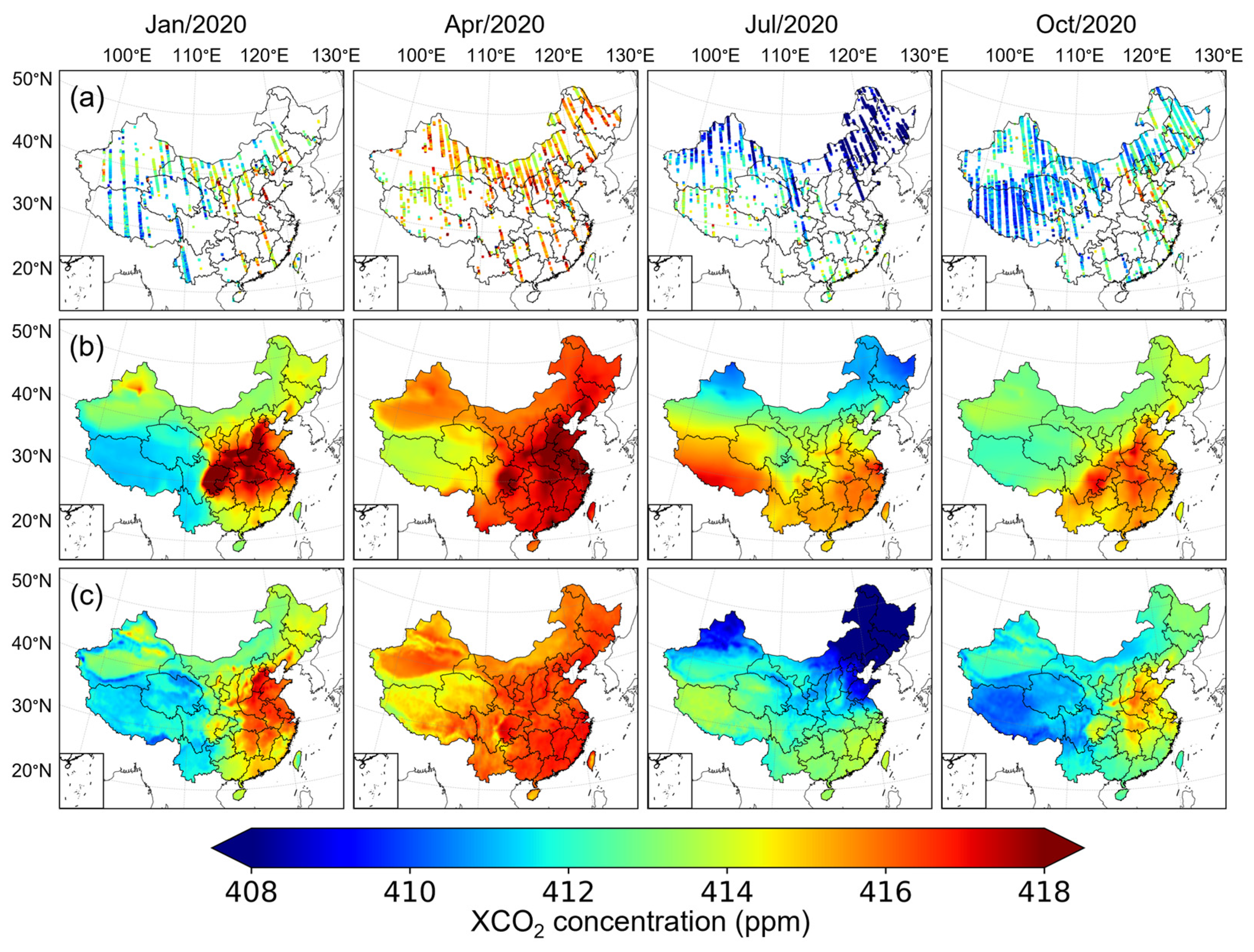
To illustrate the reconstruction capability, Figure 5 presents a comparative visualization of XCO₂ spatial distributions on four representative months in 2020 (January, April, July, and October), corresponding to winter, spring, summer, and autumn, respectively. The raw OCO-2 observations (Figure 5a) are confined to narrow along-track swaths due to orbital geometry and cloud screening, resulting in sparse spatial coverage that precludes direct characterization of nationwide XCO₂ patterns. The CAMS reanalysis product (Figure 5b), while providing spatially complete concentration fields, exhibits overly smooth gradients owing to inherent constraints in model resolution, physical parameterization schemes, and data assimilation strategies. In addition, CAMS tends to show relatively elevated concentration levels in some months. Although CAMS captures the broad-scale seasonal structure, it is less capable of resolving fine-scale spatial heterogeneity around urban agglomerations, localized emission hotspots, and transitional zones.

Figure 5. Spatial comparison of monthly XCO₂ distributions over China for four representative months in 2020 (January, April, July, and October): (a) monthly OCO-2 observation points; (b) monthly mean CAMS fields; and (c) monthly mean Air-Transformer reconstruction results.

The Air-Transformer reconstructions (Figure 5c) generally preserve the large-scale concentration patterns shown by CAMS, while exhibiting significantly enhanced spatial heterogeneity and sharper regional contrasts. In the vicinity of the monthly OCO-2 tracks, the reconstructed fields maintain high consistency with the original retrievals, demonstrating the model’s fidelity under observational constraints. Notably, compared to CAMS, the high anomalies identified by Air-Transformer are more concentrated, and the spatial transition between central and western China is more distinct. In July and October, the reconstructed fields exhibit lower concentration levels and clearer regional gradients than the reanalysis product, indicating that the relatively elevated values in CAMS are reduced. The July and October reconstructions effectively capture lower concentration levels, suggesting that the elevated bias tendency in the reanalysis product is reduced [37]. By integrating CAMS background information with OCO-2 observations constraints and multi-source environmental predictors, the Air-Transformer successfully bridges the spatiotemporal gaps of satellite data while mitigating the excessive smoothness inherent in reanalysis products, thereby providing a spatiotemporally continuous foundation for investigating XCO₂ variability and its driving mechanisms over China.

3.2. XCO₂ Spatial and Temporal Pattern Analysis

This study employed the Air-Transformer model to construct a full-coverage daily XCO₂ concentration dataset over China spanning 2015–2020, filling OCO-2 data gaps resulting from orbital coverage and cloud screening. Based on this dataset, the following section explores the spatiotemporal distribution characteristics of XCO₂ by season and region.

3.2.1. Temporal Distribution and Heterogeneity of XCO₂

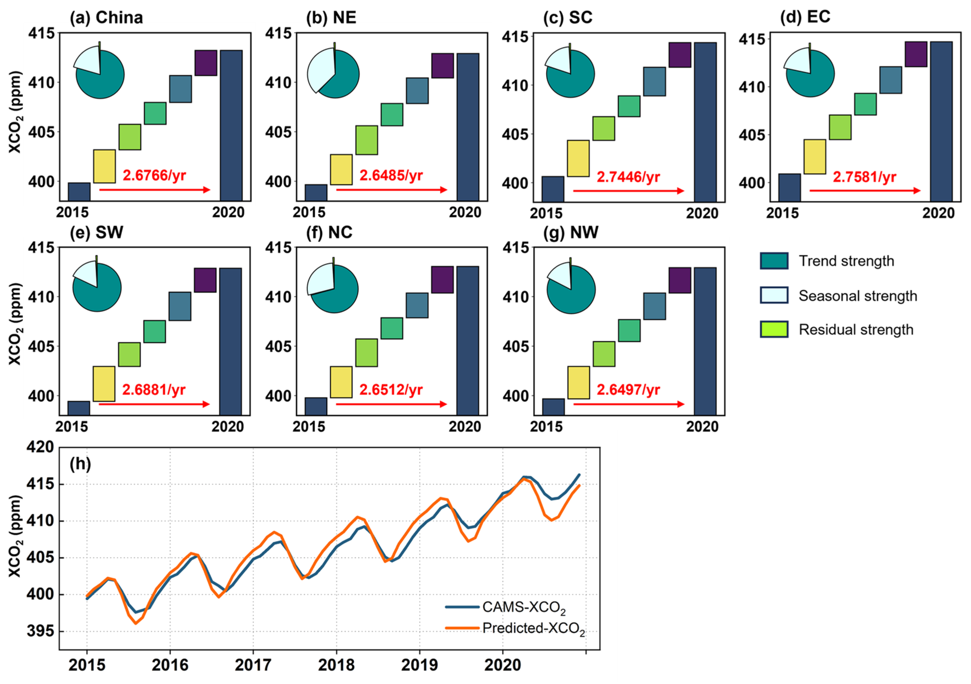
Mann–Kendall tests confirmed statistically significant upward trends in XCO₂ across all regions during 2015–2020 (p < 0.05). The national mean concentration increased from 399.83 ± 0.44 ppm (2015) to 413.21 ± 0.86 ppm (2020), exhibiting synchronized interannual variability of phase-aligned peaks and troughs across regions [17,23,25]. A distinct intra-annual pattern was observed with concentrations peaking in April and reaching a minimum in August. Notably, while the general trends are consistent, the model predictions display sharper seasonal dynamics than the smoother CAMS background field, with more pronounced drawdowns during the summer months (Figure 6h). The discrepancies are particularly evident in 2020, when the inventory-driven CAMS field may not have fully captured the abrupt emission perturbations associated with the COVID-19 lockdown period [37].

Figure 6. (a–g) Annual increases in XCO₂ for the nation and each subregion, with mean growth rates (units: ppm yr⁻¹) highlighted in red arrow lines. Inset pie charts represent the relative contributions (%) of trend, seasonal, and residual components obtained from STL decomposition. (h) Time series of XCO₂ concentrations during 2015–2020 of predicted XCO₂ and CAMS XCO₂.

Annual growth rates are consistent across regions, ranging from 2.65 ppm yr⁻¹ in NE to 2.76 ppm yr⁻¹ in EC, with a national average of 2.68 ppm yr⁻¹ (Figure 6a–g). These rates uniformly exceed the global average of 2.44 ppm yr⁻¹ [3]. This estimate is also broadly comparable to previous reconstruction-based estimates over China and East Asia, which reported growth rates ranging from 2.49 ppm yr⁻¹ to 2.66 ppm yr⁻¹ [45,46,47]. These generally consistent yet slightly different estimates may reflect differences in spatial coverage, input data sources, model structure, and the stronger anthropogenic emission background in China [24]. The 2015–2016 rate was notably higher (+0.86 ppm above the trend), largely attributed to El Niño-induced weakening of the global terrestrial carbon sink [46]. In contrast, 2017–2018 exhibited the slowest growth rate (−0.47 ppm above the trend), which may partly reflect the effects of strengthened environmental protection policies and emission control measures [48].

STL decomposition further reveals that the dominant driver of rising XCO₂ concentrations is the systematic and persistent long-term trend (trend strength: 0.67–0.91), explaining 62.6–83.1% of total variability. Seasonal strength plays a secondary role in the overall increase, being strongest in NE (0.40) and NC (0.31), reflecting relatively pronounced seasonal fluctuations. Residual strength remains universally negligible across all regions, indicating limited influence from random factors or unmodeled variability beyond the long-term trend and seasonality (Table S2).

3.2.2. Spatial Distribution and Heterogeneity of XCO₂

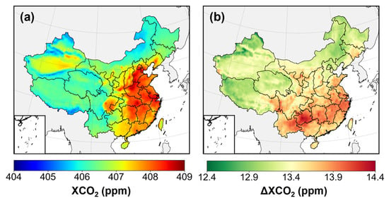
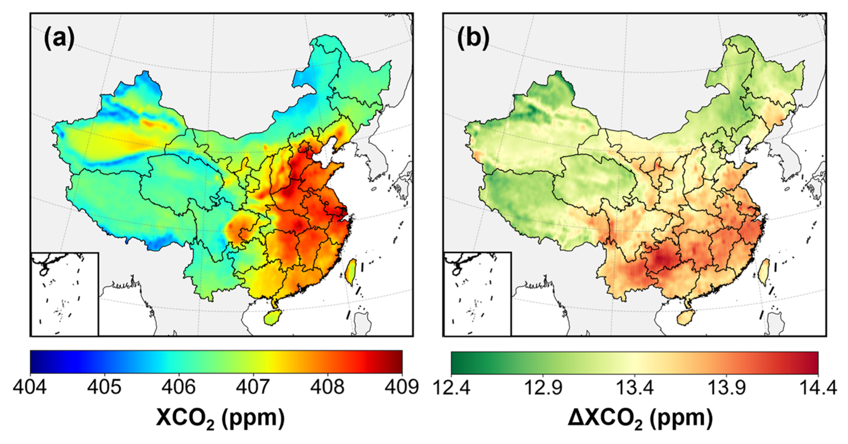
The national mean XCO₂ concentration during 2015–2020 was 406.77 ± 0.77 ppm, slightly above the global mean for the same period (406.34 ppm) [3]. Figure 7a shows the six-year mean distribution, characterized by a pronounced east–west gradient with higher values in eastern China and lower values in the west, broadly consistent with the Heihe–Tengchong line [49]. Concentrations are markedly higher in the densely populated and industrialized east and lower in the west, where strong biospheric uptake and limited anthropogenic emissions prevail. Specifically, high values cluster over the Yangtze River Delta, Beijing–Tianjin–Hebei (BTH), central China, the Sichuan Basin, and Shenyang with its surrounding urban belt, while low values occur in parts of the northeast and western high-altitude, low-population regions such as the Tibetan Plateau and remote regions. Total XCO₂ increments over 2015–2020 range from 12.43 to 14.38 ppm, revealing a more significant growth in southern China (Figure 7b). Notably, the BTH region, despite its high average concentrations, falls within a relatively low-growth tier. Previous studies suggest that Beijing and Tianjin have shown a degree of decoupling between carbon emissions and economic growth [50]. While this pattern can be partly attributed to the baseline effects [51], it may also be associated with post-industrial transitions, industrial upgrading, and stringent mitigation in megacities that reduce emission intensity [52].

Figure 7. Spatial distribution of XCO₂ concentrations at 0.1° spatial resolution across China. (a) Six-year mean (2015–2020). (b) Spatial pattern of total XCO₂ increment over the same period.

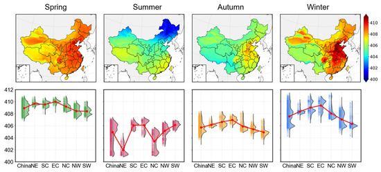
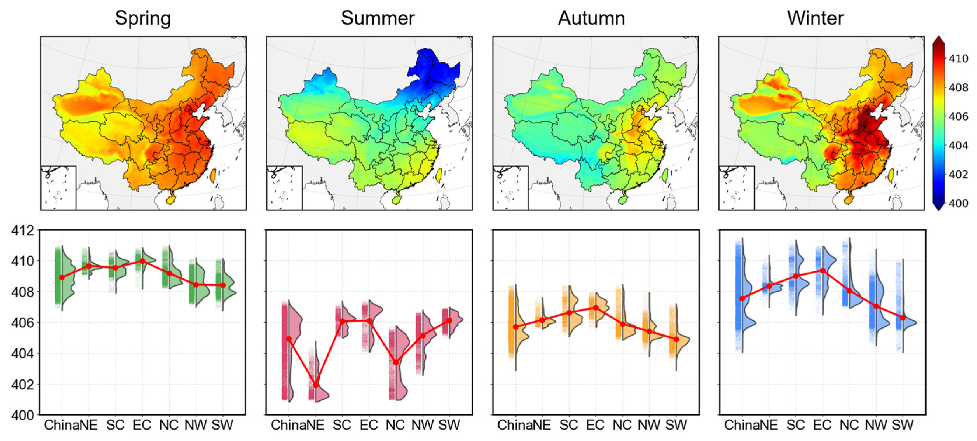
Figure 8 delineates the seasonal dynamics and regional heterogeneity of XCO₂ across China. Nationally, XCO₂ concentrations are highest in spring (408.90 ± 0.81 ppm) and winter (407.55 ± 1.39 ppm), and lower in summer (404.93 ± 1.62 ppm) and autumn (405.69 ± 0.86 ppm). Summer experiences significantly depressed concentrations, driven by enhanced photosynthetic activity during vigorous vegetation growth, which substantially fixes atmospheric CO₂ [53]. In autumn, although photosynthetic activity declines, the accumulated biomass and residual carbon uptake maintain relatively low concentrations. During winter, weakened respiration and photosynthesis shift ecosystems toward net carbon sources. Moreover, extensive coal combustion for heating in northern China increases CO₂ emissions. As weak atmospheric convection under low temperatures favors accumulation, the atmospheric CO₂ concentration peaks in spring [46].

Figure 8. Seasonal mean distribution of XCO₂ concentrations (unit: ppm) and corresponding subregional mean comparisons (red dots represent mean values; scatter plots are on the left, and violin plots on the right).

Distinct seasonal contrasts differ by regions despite the overarching national pattern. In spring, regional means are similar, with slightly higher values in NE and EC and lower in NW and SW. By contrast, winter exhibits the largest regional spread, with EC, SC, and the BTH area significantly exceeding other regions, while SW displays the lowest values. In summer, a north-low/south-high configuration emerges (Figure S4), featuring reduced values in NE and NC. The comparatively smaller summer concentration decline on the Tibetan Plateau likely stems from air transportation from the Indian Peninsula [51]. In autumn, eastern and southern means are slightly higher than western and northern values, with hot spots concentrated in central and eastern China, peaking near BTH, Wuhan, Zhengzhou, and Shijiazhuang. Mechanistically, human-activity-intensive regions (e.g., EC, NC) show stronger seasonal responses, characterized by sharp winter increases and pronounced summer decreases, whereas ecologically dominated regions (e.g., NW, SW) exhibit more stable seasonal behavior.

3.3. SHAP-Based Analysis of Driving Factors

3.3.1. Variable Correlation and Interpretability

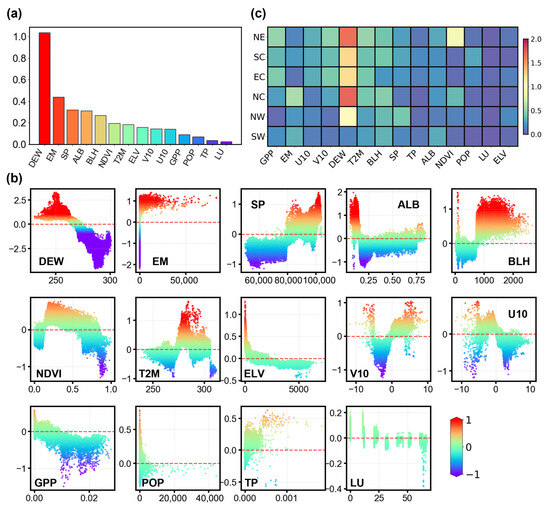
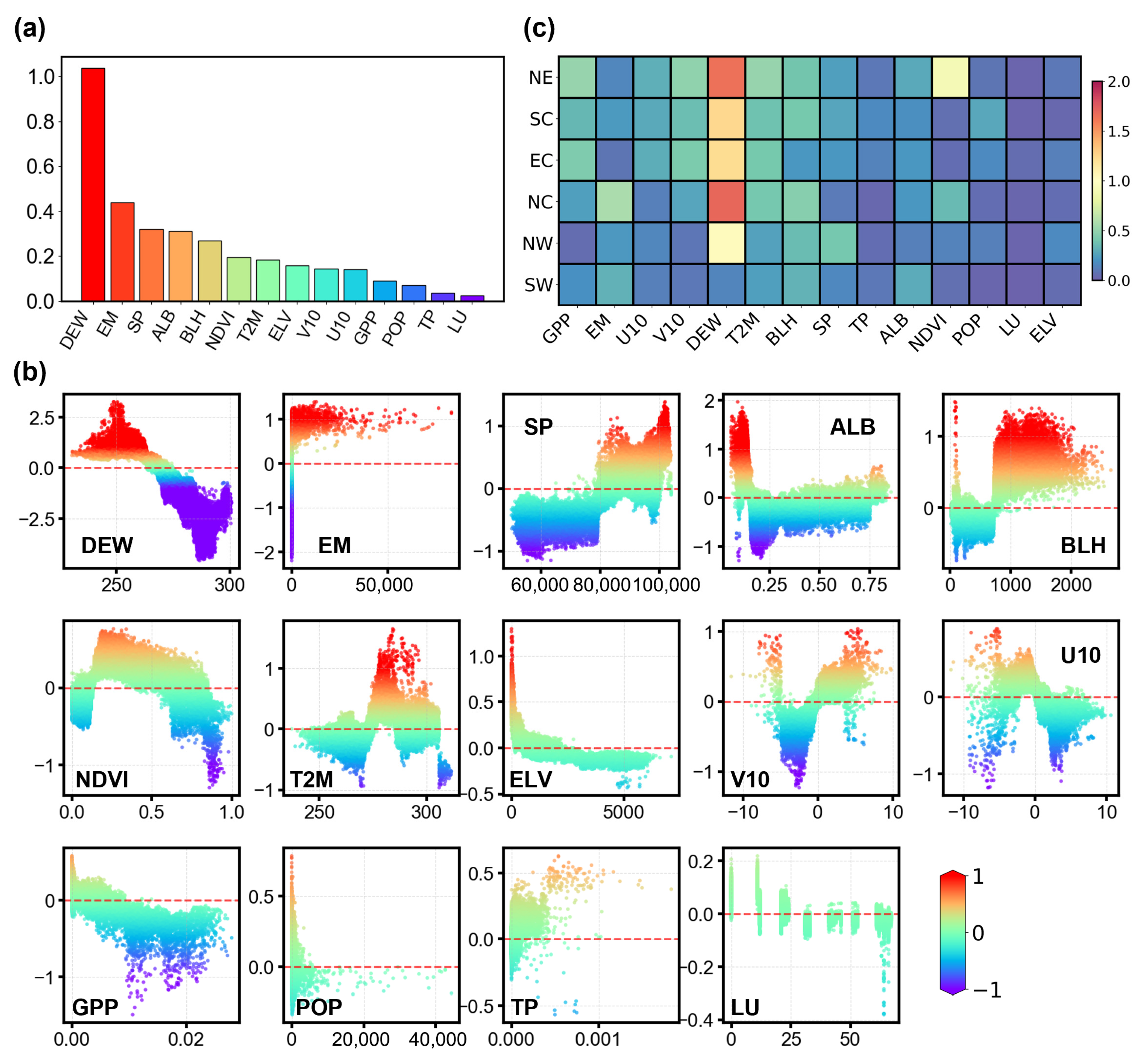
This study employed the SHAP framework to quantify the relative contributions of environmental variables to modeled XCO₂ across China. Ranked by mean absolute SHAP values (|SHAP|), DEW shows the highest contribution to model predictions, consistent with previous studies [23,25], followed by EM, SP, ALB, BLH, and NDVI (Figure 9a). To reduce potential bias in interpretation, we further examined the correlations among input variables. The correlation matrix shows that the vast majority of variable pairs have correlation coefficients below 0.8 (Figure S5), suggesting that no severe multicollinearity is present, although moderate correlations among some meteorological and ecological variables remain.

Figure 9. (a) Feature importance ranking based on the mean (|SHAP value|) for XCO₂ prediction; (b) SHAP dependence scatter plots illustrating the influence of individual environmental variables on XCO₂ predictions; (c) spatial heterogeneity heatmap of |SHAP| values for each variable across the six regions. Color intensity indicates the magnitude of the value.

DEW, NDVI, GPP, and ELV show overall negative associations with XCO₂ concentrations (Figure 9b). In the model, DEW can be interpreted as an integrated proxy for hydroclimatic conditions, seasonal variability, vegetation activity, and associated atmospheric mixing states. Therefore, its negative SHAP response may reflect the fact that humid conditions in many parts of China are often accompanied by enhanced vegetation growth and stronger ecosystem carbon uptake during the growing season [54,55]. Similarly, higher NDVI and GPP values indicate more vigorous vegetation growth and stronger photosynthetic carbon uptake, thereby contributing to lower atmospheric CO₂ concentrations [56,57]. ELV also shows a negative contribution to XCO₂. High-elevation regions in western China are generally characterized by lower anthropogenic emission intensity and stronger atmospheric ventilation, which together limit the accumulation of column CO₂ [58].

Conversely, EM shows a clear positive association with XCO₂. As a direct indicator of anthropogenic carbon emissions from fossil-fuel combustion, industrial activity, and land-use change, higher EM values correspond to elevated XCO₂ concentrations, particularly over densely populated and industrialized regions [59,60]. This result is consistent with the spatial heterogeneity of emission intensity across China and highlights the dominant role of anthropogenic sources in shaping the overall XCO₂ distribution.

Meanwhile, XCO₂ is also strongly influenced by atmospheric physical processes, including boundary layer dynamics, large-scale transport, and surface conditions [61,62,63,64]. SP exhibits a positive relationship with XCO₂, which is largely governed by topographic constraints. Prior studies identified that the interaction between elevation and surface pressure exerts a dominant influence on XCO₂ variations [45]. Specifically, higher surface pressure characterizes low-altitude regions, which naturally facilitate atmospheric accumulation and overlap with source areas, thereby driving the positive correlation [65]. The effects of ALB and T2M display non-linear patterns, reflecting their roles in modulating surface energy balance, seasonal background conditions, ecosystem activity, and anthropogenic energy use [66]. Wind fields (U10 and V10) further demonstrate non-linear behavior, indicating the importance of horizontal transport.

To further distinguish the drivers of XCO₂ levels from those associated with its long-term increase, we additionally compared the SHAP values of individual predictors between 2015 and 2020 (Figure S6). The results show that the temporal changes in SHAP contributions differ substantially among variables. In particular, emission-related factors (EM) exhibit the largest positive change, suggesting that anthropogenic emissions play the dominant role in the modeled increase in XCO₂ over the study period. DEW also shows a pronounced positive change in SHAP value, indicating that hydroclimatic conditions and the associated seasonal–ecological state remain important in shaping the temporal evolution of XCO₂ within the model framework. By contrast, some variables, such as T2M and V10, display negative changes in SHAP contributions.

3.3.2. Regional Heterogeneity of Driving Mechanisms

Figure 9c highlights marked spatial heterogeneity in the SHAP contributions of different factors to XCO₂ across China. Although DEW ranks first in the other regions, SW exhibits notably lower SHAP values for DEW. This may be associated with the persistently humid climate in SW, where relatively stable atmospheric moisture conditions could reduce the sensitivity of modeled XCO₂ to humidity fluctuations. In NW, ELV ranks higher than in other regions, driven by sharp terrain transitions from basins to plateaus. The strong influence of atmospheric transport suggests a high potential for dilution [67]. Development strategies here should leverage the abundant wind and solar resources to substitute local fossil fuel consumption.

NE exhibits the highest SHAP contributions from GPP and NDVI nationwide. This pattern may be related to the extensive forest carbon sink in NE [67], which likely enhances seasonal photosynthetic uptake and thereby influences atmospheric CO₂ variability [68]. Consequently, mitigation strategies here should prioritize enhancing the carbon sink quality rather than solely focusing on emission reduction. Specifically, further quantification of the carbon offset potential of mature forests could support the inclusion of this region in broader carbon market frameworks [69]. In NC, a major industrial and energy hub (e.g., BTH), EM stands out due to high and spatially heterogeneous emission intensities [70]. The SHAP results indicate that variations in XCO₂ are highly sensitive to emission intensity. Therefore, the primary policy may need to focus on decoupling industrial growth from carbon emissions and accelerating the electrification of winter heating systems to curb the intense seasonal peaks driven by fossil fuel combustion [71].

3.4. Limitations

Despite the high accuracy of the reconstructed XCO₂ dataset, this study has several limitations. First, the multisource input datasets differ in spatial and temporal resolution, retrieval uncertainty, and update frequency, and these discrepancies may propagate through resampling, spatiotemporal alignment, and feature fusion during the reconstruction process. Although strict quality control and multi-dimensional validation strategies partially mitigate this issue, the mechanisms of regional and seasonal error propagation require further quantitative investigation. Second, independent validation remains constrained by the sparse distribution of long-term ground-based observations, which limits a comprehensive assessment of the model’s spatial extrapolation capability. In addition, although the SHAP-based interpretation framework provides valuable information on the relative contributions of input variables, it remains a data-driven interpretation of the model and still lacks a physical explanation of the relationships among variables in the real-world atmospheric system. To address these limitations, future work will focus on integrating process-based chemical transport models with deep learning to enhance physical consistency. We also plan to incorporate multisource satellite observations to improve spatiotemporal coverage and further reduce uncertainty.

4. Conclusions

This study introduced Air-Transformer, a transformer-based deep learning method integrating dual self-attention mechanisms, for reconstructing a daily seamless XCO₂ dataset over China during 2015–2020. By modeling long-range dependencies and non-linear variable interactions based on OCO-2 retrievals and multi-source auxiliary data, this approach overcomes the limitations of sparse satellite observations and inventories. The model achieves high accuracy (R² = 0.98) and demonstrates robust generalization capabilities across different spatiotemporal scales. Our analysis reveals a significant increasing trend in XCO₂ (2.68 ppm yr⁻¹), characterized by a persistent east-high/west-low and spring-high/summer-low pattern. Coupling Air-Transformer outputs with SHAP analysis identifies DEW, EM, and SP as the dominant drivers, exhibiting strong regional heterogeneity. These findings provide specific, data-driven insights for formulating differentiated regional carbon mitigation strategies.

References

- Bruhwiler, L.; Basu, S.; Butler, J.H.; Chatterjee, A.; Dlugokencky, E.; Kenney, M.A.; McComiskey, A.; Montzka, S.A.; Stanitski, D. Observations of Greenhouse Gases as Climate Indicators. Clim. Change 2021, 165, 12. [Google Scholar] [CrossRef] [Scilit]
- Kump, L.R. What Drives Climate? Nature 2000, 408, 651–652. [Google Scholar] [CrossRef] [Scilit] [PubMed]
- Lan, X.; Tans, P.K.W. Thoning Trends in Globally-Averaged CO2 Determined from NOAA Global Monitoring Laboratory Measurements. Version 2025-06. Available online: https://gml.noaa.gov/ccgg/trends/global.html?doi=10.15138/9n0h-zh07 (accessed on 27 June 2025).
- Hotchkiss, E.R.; Hall, R.O., Jr.; Sponseller, R.A.; Butman, D.; Klaminder, J.; Laudon, H.; Rosvall, M.; Karlsson, J. Sources of and Processes Controlling CO2 Emissions Change with the Size of Streams and Rivers. Nat. Geosci. 2015, 8, 696–699. [Google Scholar] [CrossRef] [Scilit]
- Masson-Delmotte, V.; Zhai, P.; Pirani, A.; Connors, S.L.; Pean, C.; Berger, S.; Caud, N.; Chen, Y.; Goldfarb, L.; Gomis, M.I.; et al. IPCC 2021. Summary for Policymakers. Climate Change 2021: The Physical Science Basis. Contribution of Working Group I to the Sixth Assessment Report of the Intergovernmental Panel on Climate Change; Cambridge University Press: Cambridge, UK; New York, NY, USA, 2023; pp. 3–32. [Google Scholar]
- IEA. Global Energy Review 2025; IEA: Paris, France, 2025. [Google Scholar]
- Joint Research Centre–European Commission. Fossil CO2 Emissions of All World Countries: 2018 Report; Publications Office: Brussels, Belgium, 2018. [Google Scholar]
- Zhao, R.; Zhan, L.; Yao, M.; Yang, L. A Geographically Weighted Regression Model Augmented by Geodetector Analysis and Principal Component Analysis for the Spatial Distribution of PM2.5. Sustain. Cities Soc. 2020, 56, 102106. [Google Scholar] [CrossRef] [Scilit]
- Liu, Z.; Deng, Z.; He, G.; Wang, H.; Zhang, X.; Lin, J.; Qi, Y.; Liang, X. Challenges and Opportunities for Carbon Neutrality in China. Nat. Rev. Earth Environ. 2022, 3, 141–155. [Google Scholar] [CrossRef] [Scilit]
- Zeng, Q.; Ma, F.; Lu, X.; Xu, W. Policy Uncertainty and Carbon Neutrality: Evidence from China. Financ. Res. Lett. 2022, 47, 102771. [Google Scholar] [CrossRef] [Scilit]
- Zhang, T.; Zhang, W.; Yang, R.; Liu, Y.; Jafari, M. CO2 Capture and Storage Monitoring Based on Remote Sensing Techniques: A Review. J. Clean. Prod. 2021, 281, 124409. [Google Scholar] [CrossRef] [Scilit]
- Crisp, D.; Atlas, R.M.; Breon, F.-M.; Brown, L.R.; Burrows, J.P.; Ciais, P.; Connor, B.J.; Doney, S.C.; Fung, I.Y.; Jacob, D.J.; et al. The Orbiting Carbon Observatory (OCO) Mission. Adv. Space Res. 2004, 34, 700–709. [Google Scholar] [CrossRef] [Scilit]
- Eldering, A.; Wennberg, P.O.; Crisp, D.; Schimel, D.S.; Gunson, M.R.; Chatterjee, A.; Liu, J.; Schwandner, F.M.; Sun, Y.; O’Dell, C.W.; et al. The Orbiting Carbon Observatory-2 Early Science Investigations of Regional Carbon Dioxide Fluxes. Science 2017, 358, eaam5745. [Google Scholar] [CrossRef] [Scilit]
- Hamazaki, T.; Kuze, A.; Kondo, K. Sensor System for Greenhouse Gas Observing Satellite (GOSAT). In Proceedings of the Infrared Spaceborne Remote Sensing XII; Strojnik, M., Ed.; SPIE: Denver, CO, USA, 2004; Volume 5543, p. 275. [Google Scholar]
- Liu, Y.; Wang, J.; Yao, L.; Chen, X.; Cai, Z.; Yang, D.; Yin, Z.; Gu, S.; Tian, L.; Lu, N.; et al. The TanSat Mission: Preliminary Global Observations. Sci. Bull. 2018, 63, 1200–1207. [Google Scholar] [CrossRef] [Scilit]
- Crisp, D.; Pollock, H.R.; Rosenberg, R.; Chapsky, L.; Lee, R.A.M.; Oyafuso, F.A.; Frankenberg, C.; O’Dell, C.W.; Bruegge, C.J.; Doran, G.B.; et al. The On-Orbit Performance of the Orbiting Carbon Observatory-2 (OCO-2) Instrument and Its Radiometrically Calibrated Products. Atmos. Meas. Tech. 2017, 10, 59–81. [Google Scholar] [CrossRef] [Scilit]
- He, Q.; Ye, T.; Chen, X.; Dong, H.; Wang, W.; Liang, Y.; Li, Y. Full-Coverage Mapping High-Resolution Atmospheric CO2 Concentrations in China from 2015 to 2020: Spatiotemporal Variations and Coupled Trends with Particulate Pollution. J. Clean. Prod. 2023, 428, 139290. [Google Scholar] [CrossRef] [Scilit]
- Chen, W.; Ren, T.; Zhao, C.; Wen, Y.; Gu, Y.; Zhou, M.; Wang, P. Transformer-Based Fast Mole Fraction of CO2 Retrievals from Satellite-Measured Spectra. J. Remote Sens. 2025, 5, 0470. [Google Scholar] [CrossRef] [Scilit]
- Wei, W.; Bao, Z.; Su, Y.; Wang, P.; Bai, S. Research of Rapid Retrieving Models for GOSAT XCO2 Based on Machine Learning. Comput. Geosci. 2025, 29, 35. [Google Scholar] [CrossRef] [Scilit]
- Zhang, W.; Wang, Z.; Li, T.; Li, B.; Li, Y.; Han, Z. Random Forest-Based Retrieval of XCO2 Concentration from Satellite-Borne Shortwave Infrared Hyperspectral. Atmosphere 2025, 16, 238. [Google Scholar] [CrossRef] [Scilit]
- Hu, K.; Liu, Z.; Shao, P.; Ma, K.; Xu, Y.; Wang, S.; Wang, Y.; Wang, H.; Di, L.; Xia, M.; et al. A Review of Satellite-Based CO2 Data Reconstruction Studies: Methodologies, Challenges, and Advances. Remote Sens. 2024, 16, 3818. [Google Scholar] [CrossRef] [Scilit]
- Miao, Y.; Zou, M.; Sheng, S.; Zhu, K. CO2 Satellite Inversion Methocl Based on Machine Learning. China Environ. Sci. 2023, 43, 20–27. [Google Scholar]
- He, C.; Ji, M.; Li, T.; Liu, X.; Tang, D.; Zhang, S.; Luo, Y.; Grieneisen, M.L.; Zhou, Z.; Zhan, Y. Deriving Full-Coverage and Fine-Scale XCO2 Across China Based on OCO-2 Satellite Retrievals and CarbonTracker Output. Geophys. Res. Lett. 2022, 49, e2022GL098435. [Google Scholar] [CrossRef] [Scilit]
- Wang, J. Global Daily 1 Km Gapless XCO2 (2003−2023) Derived from Multi-Satellite Observations and a Spatiotemporal Deep Learning Framework. Environ. Impact Assess. Rev. 2026, 117, 108146. [Google Scholar] [CrossRef] [Scilit]
- Wu, C.; Yang, S.; Jiao, D.; Chen, Y.; Yang, J.; Huang, B. Estimation of Daily XCO2 at 1 Km Resolution in China Using a Spatiotemporal ResNet Model. Sci. Total Environ. 2024, 954, 176171. [Google Scholar] [CrossRef] [Scilit] [PubMed]
- Shao, W.; Yue, T.; Zhang, L.; Tian, W.; Wang, H.; Zhou, H.; Wu, C.; Zhang, L. Mapping Daily 1-Km Resolution XCO2 in China Using Deep Learning and Multi-Source Data. Resour. Conserv. Recycl. 2026, 227, 108755. [Google Scholar] [CrossRef] [Scilit]
- Cui, B.; Liu, M.; Li, S.; Jin, Z.; Zeng, Y.; Lin, X. Deep Learning Methods for Atmospheric PM2.5 Prediction: A Comparative Study of Transformer and CNN-LSTM-Attention. Atmos. Pollut. Res. 2023, 14, 101833. [Google Scholar] [CrossRef] [Scilit]
- Zou, R.; Huang, H.; Lu, X.; Zeng, F.; Ren, C.; Wang, W.; Zhou, L.; Dai, X. PD-LL-Transformer: An Hourly PM2.5 Forecasting Method over the Yangtze River Delta Urban Agglomeration, China. Remote Sens. 2024, 16, 1915. [Google Scholar] [CrossRef] [Scilit]
- Vaswani, A.; Shazeer, N.; Parmar, N.; Uszkoreit, J.; Jones, L.; Gomez, A.N.; Kaiser, L.; Polosukhin, I. Attention Is All You Need. arXiv 2023, arXiv:1706.03762. [Google Scholar]
- Han, Z.; Wang, H.; Wu, J.; Shu, Y.; Luo, X.; Wang, Z.; Hu, Y.; Wei, Z.; Xu, T.; Fan, Z. Spatial Heterogeneity and Evolutionary Pathways of PM2.5 Pollution Driven by Urbanization in China to 2100. Environ. Res. 2026, 290, 123512. [Google Scholar] [CrossRef] [Scilit] [PubMed]
- Yao, T.; Lu, S.; Wang, Y.; Li, X.; Ye, H.; Duan, Y.; Fu, Q.; Li, J. Revealing the Drivers of Surface Ozone Pollution by Explainable Machine Learning and Satellite Observations in Hangzhou Bay, China. J. Clean. Prod. 2024, 440, 140938. [Google Scholar] [CrossRef] [Scilit]
- Liu, X.; Lu, D.; Zhang, A.; Liu, Q.; Jiang, G. Data-Driven Machine Learning in Environmental Pollution: Gains and Problems. Environ. Sci. Technol. 2022, 56, 2124–2133. [Google Scholar] [CrossRef] [Scilit]
- Li, M.; Liu, H.; Geng, G.; Hong, C.; Liu, F.; Song, Y.; Tong, D.; Zheng, B.; Cui, H.; Man, H.; et al. Anthropogenic Emission Inventories in China: A Review. Natl. Sci. Rev. 2017, 4, 834–866. [Google Scholar] [CrossRef] [Scilit]
- Jeong, S.; Ryu, Y.; Gentine, P.; Lian, X.; Fang, J.; Li, X.; Dechant, B.; Kong, J.; Choi, W.; Jiang, C.; et al. Persistent Global Greening over the Last Four Decades Using Novel Long-Term Vegetation Index Data with Enhanced Temporal Consistency. Remote Sens. Environ. 2024, 311, 114282. [Google Scholar] [CrossRef] [Scilit]
- Inness, A.; Ades, M.; Agustí-Panareda, A.; Barré, J.; Benedictow, A.; Blechschmidt, A.-M.; Dominguez, J.J.; Engelen, R.; Eskes, H.; Flemming, J.; et al. The CAMS Reanalysis of Atmospheric Composition. Atmos. Chem. Phys. 2019, 19, 3515–3556. [Google Scholar] [CrossRef] [Scilit]
- Guan, X.; Sun, Z.; Chu, D.; Xie, G.; Wang, Y.; Shen, H. Long-Term (2000–2020) Global 0.05° Continuous Atmospheric Carbon Dioxide Mapping Combining OCO-2 Observations and Model Simulations. Sci. Total Environ. 2024, 957, 177051. [Google Scholar] [CrossRef] [Scilit]
- Wang, Y.; Yuan, Q.; Li, T.; Yang, Y.; Zhou, S.; Zhang, L. Seamless Mapping of Long-Term (2010–2020) Daily Global XCO2 and XCH4 from the Greenhouse Gases Observing Satellite (GOSAT), Orbiting Carbon Observatory 2 (OCO-2), and CAMS Global Greenhouse Gas Reanalysis (CAMS-EGG4) with a Spatiotemporally Self-Supervised Fusion Method. Earth Syst. Sci. Data 2023, 15, 3597–3622. [Google Scholar] [CrossRef] [Scilit]
- Tao, C.; Peng, Y.; Zhang, Q.; Zhang, Y.; Gong, B.; Wang, Q.; Wang, W. Diagnosing Ozone–NOx–VOC–Aerosol Sensitivity and Uncovering Causes of Urban–Nonurban Discrepancies in Shandong, China, Using Transformer-Based Estimations. Atmos. Chem. Phys. 2024, 24, 4177–4192. [Google Scholar] [CrossRef] [Scilit]
- Tao, C.; Zhang, Y.; Zhang, X.; Guan, X.; Peng, Y.; Wang, G.; Zhang, Q.; Ren, Y.; Zhao, X.; Zhao, R.; et al. Discrepant Global Surface Ozone Responses to Emission- and Heatwave-Induced Regime Shifts. Environ. Sci. Technol. 2024, 58, 22288–22297. [Google Scholar] [CrossRef] [Scilit]
- Wunch, D.; Wennberg, P.O.; Osterman, G.; Fisher, B.; Naylor, B.; Roehl, C.M.; O’Dell, C.; Mandrake, L.; Viatte, C.; Kiel, M.; et al. Comparisons of the Orbiting Carbon Observatory-2 (OCO-2) XCO2 Measurements with TCCON. Atmos. Meas. Tech. 2017, 10, 2209–2238. [Google Scholar] [CrossRef] [Scilit]
- Labzovskii, L.D.; Kenea, S.T.; Lindqvist, H.; Kim, J.; Li, S.; Byun, Y.-H.; Goo, T.-Y. Towards Robust Calculation of Interannual CO2 Growth Signal from TCCON (Total Carbon Column Observing Network). Remote Sens. 2021, 13, 3868. [Google Scholar] [CrossRef] [Scilit]
- Chen, C.; Chen, X.; Liu, Q.; Zhang, W.; Chen, Y.; Ou, Y.; Liu, X.; Yang, H. Estimation and Analysis of CO2 Column Concentrations (XCO2) in the Yangtze River Delta of China Based on Multi-Source Data and Machine Learning. Atmos. Pollut. Res. 2025, 16, 102528. [Google Scholar] [CrossRef] [Scilit]
- Lundberg, S.; Lee, S.-I. A Unified Approach to Interpreting Model Predictions. arXiv 2017, arXiv:1705.07874. [Google Scholar] [CrossRef] [Scilit]
- Mitchell, R.; Frank, E.; Holmes, G. GPUTreeShap: Massively Parallel Exact Calculation of SHAP Scores for Tree Ensembles. PeerJ Comput. Sci. 2022, 8, e880. [Google Scholar] [CrossRef] [Scilit]
- Geng, Y.; Du, N.; Wang, L.; Deng, X.; Zuo, Y.; Qian, L.; Zhu, W. High-Resolution Reconstruction and Driving Mechanism Analysis of XCO2 over Mainland China Based on the GAM-Optuna-ERT Model. Atmos. Res. 2026, 334, 108677. [Google Scholar] [CrossRef] [Scilit]
- Li, Y.; Yan, J.; Zhong, L.; Bao, D.; Sun, L.; Li, G. Full-Coverage Mapping of Daily High-Resolution XCO2 across China from 2015 to 2020 by Deep Learning-Based Spatio-Temporal Fusion. IEEE Trans. Geosci. Remote Sens. 2025, 63, 4102716. [Google Scholar] [CrossRef] [Scilit]
- Te, T.; Bao, C.; Bagan, H.; Xie, Y.; Che, M.; Yoshida, T.; Uudus, B. Mapping Seamless Monthly XCO2 in East Asia: Utilizing OCO-2 Data and Machine Learning. Int. J. Appl. Earth Obs. Geoinf. 2024, 133, 104117. [Google Scholar] [CrossRef] [Scilit]
- Hu, K.; Liu, Z.; Shao, P. High-Resolution Spatiotemporal Estimation of XCO2 Concentration Using Carbon Satellite Data. Trans. Atmos. Sci. 2024, 47, 976–992. [Google Scholar] [CrossRef]
- Li, T.; Wu, J.; Wang, T. Generating Daily High-Resolution and Full-Coverage XCO2 across China from 2015 to 2020 Based on OCO-2 and CAMS Data. Sci. Total Environ. 2023, 893, 164921. [Google Scholar] [CrossRef] [Scilit]
- Hu, M.; Li, X.; Song, M.; Yang, L.; Yuan, Y. China Province-by-Province Carbon Neutrality Roadmap Analysis: Challenges and Opportunities; Institute for Global Decarbonization Progress (iGDP): Beijing, China, 2024. [Google Scholar]
- He, J.; Wang, W.; Wang, N. Seamless Reconstruction and Spatiotemporal Analysis of Satellite-Based XCO2 Incorporating Temporal Characteristics: A Case Study in China during 2015–2020. Adv. Space Res. 2024, 74, 3804–3825. [Google Scholar] [CrossRef] [Scilit]
- Li, S.; Zhang, X.; Deng, Z.; Liu, K.; Wang, J.; Fan, J. Widening Inequality: Diverging Trends in CO2 and Air Pollutant Emissions across Chinese Cities. Resour. Environ. Sustain. 2025, 21, 100227. [Google Scholar] [CrossRef] [Scilit]
- Chang, Z.; Fan, L.; Wigneron, J.-P.; Wang, Y.-P.; Ciais, P.; Chave, J.; Fensholt, R.; Chen, J.M.; Yuan, W.; Ju, W.; et al. Estimating Aboveground Carbon Dynamic of China Using Optical and Microwave Remote-Sensing Datasets from 2013 to 2019. J. Remote Sens. 2023, 3, 0005. [Google Scholar] [CrossRef] [Scilit]
- Falahatkar, S.; Mousavi, S.M.; Farajzadeh, M. Spatial and Temporal Distribution of Carbon Dioxide Gas Using GOSAT Data over IRAN. Environ. Monit. Assess. 2017, 189, 627. [Google Scholar] [CrossRef] [Scilit] [PubMed]
- Yuan, Z.; Liu, Y.; Yang, A.; Wang, D. A High-Resolution Daily CO2 Dataset for China (2016–2020). Sci. Data 2026, 13, 249. [Google Scholar] [CrossRef] [Scilit]
- Liang, Z.; Tang, W.; Zeng, N.; Cai, Q. Simulation of Surface Atmospheric CO2 Concentration in Beijing-Tianjin-Hebei Region Based on WRF Model. Trans. Atmos. Sci. 2022, 45, 387–396. [Google Scholar] [CrossRef]
- Zhu, W.; Zhang, H.; Zhang, X.; Guo, H.; Liu, Y. Spatiotemporal Variation and Influencing Factors of Atmospheric CO2 Concentration in China. Chin. Geogr. Sci. 2025, 35, 149–160. [Google Scholar] [CrossRef] [Scilit]
- Hedelius, J.K.; Feng, S.; Roehl, C.M.; Wunch, D.; Hillyard, P.W.; Podolske, J.R.; Iraci, L.T.; Patarasuk, R.; Rao, P.; O’Keeffe, D.; et al. Emissions and Topographic Effects on Column CO2 Variations, with a Focus on the Southern California Megacity. J. Geophys. Res. Atmos. 2017, 122, 7200–7215. [Google Scholar] [CrossRef] [Scilit]
- Wang, W.; He, J.; Feng, H.; Jin, Z. High-Coverage Reconstruction of XCO2 Using Multisource Satellite Remote Sensing Data in Beijing–Tianjin–Hebei Region. Int. J. Environ. Res. Public Health 2022, 19, 10853. [Google Scholar] [CrossRef] [Scilit]
- Wang, Y.; Chen, G.; Yang, Y.; Zhang, Z.; Zhang, R.; Wang, P.; Zhang, H. Anthropogenic Emissions Shape Long-Term Changes in PM2.5 Concentrations and Health Risks in China. Eco-Environ. Health 2025, 4, 100198. [Google Scholar] [CrossRef] [Scilit] [PubMed]
- Sheng, M.; Lei, L.; Zeng, Z.-C.; Rao, W.; Zhang, S. Detecting the Responses of CO2 Column Abundances to Anthropogenic Emissions from Satellite Observations of GOSAT and OCO-2. Remote Sens. 2021, 13, 3524. [Google Scholar] [CrossRef] [Scilit]
- Jacobs, N.; Simpson, W.R.; Graham, K.A.; Holmes, C.; Hase, F.; Blumenstock, T.; Tu, Q.; Frey, M.; Dubey, M.K.; Parker, H.A.; et al. Spatial Distributions of XCO2 Seasonal Cycle Amplitude and Phase over Northern High-Latitude Regions. Atmos. Chem. Phys. 2021, 21, 16661–16687. [Google Scholar] [CrossRef] [Scilit]
- Dong, X.; Yue, M.; Jiang, Y.; Hu, X.-M.; Ma, Q.; Pu, J.; Zhou, G. Analysis of CO2 Spatio-Temporal Variations in China Using a Weather–Biosphere Online Coupled Model. Atmos. Chem. Phys. 2021, 21, 7217–7233. [Google Scholar] [CrossRef] [Scilit]
- Dima, C.; Adrian, R.; Rosu, B.; Constantin, D.; Arseni, M.; Georgescu, L. Evolution of NO2 in Five Major Cities in Europe Using Remote Satellite Observations and In-Situ Measurements. Ann. Univ. Dunarea Jos Galati 2016, 9, 66–70. [Google Scholar]
- Chen, X.; He, Q.; Ye, T.; Liang, Y.; Li, Y. Decoding Spatiotemporal Dynamics in Atmospheric CO2 in Chinese Cities: Insights from Satellite Remote Sensing and Geographically and Temporally Weighted Regression Analysis. Sci. Total Environ. 2024, 908, 167917. [Google Scholar] [CrossRef] [Scilit]
- Voiculescu, M.; Constantin, D.-E.; Condurache-Bota, S.; Călmuc, V.; Roșu, A.; Bălănică, C.M.D. Role of Meteorological Parameters in the Diurnal and Seasonal Variation of NO2 in a Romanian Urban Environment. Int. J. Environ. Res. Public Health 2020, 17, 6228. [Google Scholar] [CrossRef] [Scilit]
- Fu, Y.; Sun, W.; Luo, F.; Zhang, Y.; Zhang, X. Variation Patterns and Driving Factors of Regional Atmospheric CO2 Anomalies in China. Environ. Sci. Pollut. Res. 2022, 29, 19390–19403. [Google Scholar] [CrossRef] [Scilit] [PubMed]
- Li, K.; Yang, L.; Zhang, J. Monitoring and Driving Factors Analysis of CO2 Concentration in China’s Mainland Based on TanSat. China Environ. Sci. 2023, 43, 5645–5654. [Google Scholar]
- Bai, J.; Chang, I.-S.; Zhang, C.; Wu, J. Allocation of CO2 Emission Target in China under the “1 + N” Policy: Considering Natural Carbon Sinks and Wind-Solar-Hydropower Endowments. Environ. Impact Assess. Rev. 2024, 106, 107472. [Google Scholar] [CrossRef] [Scilit]
- Wang, Y.; Wang, M.; Teng, F.; Ji, Y. Remote Sensing Monitoring and Analysis of Spatiotemporal Changes in China’s Anthropogenic Carbon Emissions Based on XCO2 Data. Remote Sens. 2023, 15, 3207. [Google Scholar] [CrossRef] [Scilit]
- Hu, Y.-J.; Zhang, R.; Wang, H.; Li, C.; Tang, B.-J. Synergizing Policies for Carbon Reduction, Energy Transition and Pollution Control: Evidence from Chinese Power Generation Industry. J. Clean. Prod. 2024, 436, 140460. [Google Scholar] [CrossRef] [Scilit]
Disclaimer/Publisher’s Note: The statements, opinions and data contained in all publications are solely those of the individual author(s) and contributor(s) and not of MDPI and/or the editor(s). MDPI and/or the editor(s) disclaim responsibility for any injury to people or property resulting from any ideas, methods, instructions or products referred to in the content. |
© 2026 by the authors. Licensee MDPI, Basel, Switzerland. This article is an open access article distributed under the terms and conditions of the Creative Commons Attribution (CC BY) license.