Assessment of Forest Structure Estimation from Terrestrial LiDAR in Fire-Affected Areas

Highlights

What are the main findings?

• TLS-derived DBH remained robust across burn severities (OA = 92.1–95.0%; RMSE = 0.93–1.19 cm) in trees with moderate point loss due to reduced intensity.
• Return intensity and return density decreased with burn severity, with returns per unit trunk area reduced by 14.9% (moderate) and 54.3% (severe) relative to unburned plots.

What are the implications of the main findings?

• TLS can support reliable post-fire tree-level inventory in low-moderate severity areas, enabling accurate DBH-based structural assessments with minimal loss of precision.
• In high-severity plots, severe intensity-driven return loss reduced the number of segmentable trees and valid DBH extractions, propagating into lower plot-level AGB estimates (accuracy dropping to 74%), highlighting the need for methods robust to char-induced reflectance changes.

Abstract

This study evaluated the performance of terrestrial LiDAR (TLS) for post-fire forest inventory across two large wildfires in Spain as a function of burn severity. We analyzed tree-level diameter at breast height (DBH), plot-level above-ground biomass (AGB), and the influence of burn severity on return intensity. DBH of segmented trees was accurately retrieved across severities, with overall accuracies of 92.1%, 95.0%, and 94.4% and RMSE of 1.19, 0.94, and 0.93 cm in unburned, moderate, and severe plots, respectively (rRMSE = 7.97%, 6.46%, 6.94%). AGB showed lower agreement, with accuracies of 93%, 88%, and 74%. After adjusting by quadrant-level biomass consumption, mean post-fire AGB values were 76.29, 65.07, and 32.90 Mg ${\mathrm{h}\mathrm{a}}^{-1}$, with mean absolute errors of 4.55, 6.38, and 6.11 Mg ${\mathrm{h}\mathrm{a}}^{-1}$. Return intensity decreased with burn severity, reducing the number of returns by 14.9% in moderately burned and 54.3% in severely burned plots. These results support the use of TLS for post-fire forest inventory in low-to-moderate severity conditions. However, in high-severity plots, return intensity reduction limited tree segmentation and DBH extraction, introducing uncertainty in plot-level AGB estimation.

1. Introduction

Forests play a key role in the functioning of ecosystems, supporting biodiversity, regulating energy and water fluxes, and capturing carbon [1,2]. Their structure, often described by variables such as canopy height, fractional cover, above-ground biomass (AGB) or leaf area index (LAI), is directly linked to these processes, and it can be estimated using remote sensing [3,4]. Therefore, monitoring forest structure and biomass is essential to understand the carbon balance of forest stands [5].

Forest disturbances, particularly fire, can significantly alter the ecological functions of a forest, turning them from a carbon sink into a carbon source. Additionally, wildfires can release large amounts of gas and particulate matter, a significant source of air pollution [6] with negative impacts on the atmosphere and human health [7,8,9]. Climate trends suggest an increase in the magnitude and frequency of wildfires, as well as an increase in the duration of the fire season [10]. Even the most fire-adapted ecosystems, such as those in the Mediterranean, are beginning to suffer unprecedented consequences due to the external pressures of climate change and extreme weather events [11,12], exacerbated by the consequences of rural abandonment [13].

LiDAR technology has proven to be a versatile tool for quantifying and mapping forest structural attributes in a wide range of ecosystems. LiDAR sensors can be mounted on different platforms: satellite LiDAR, airborne LiDAR and terrestrial LiDAR (TLS). Yet, the implementation of the latter is less established in terms of large-area coverage, cost-efficiency and operational scalability compared to airborne or mobile systems [14,15]. TLS can provide highly detailed descriptions due to their very high point density, and it has been suggested that TLS measurements could replace traditional inventory techniques [15,16], offering an effective alternative for tree reconstruction in a fast and non-destructive way [17,18]. The point cloud allows the extraction of several structural variables, such as the diameter at breast height, DBH [19], leaf area index [20], canopy height [21], trunk volume [22], fuel load [23], or estimate biomass consumption [24], among others.

Despite these advantages, TLS deployment is constrained by high instrument cost, limited spatial coverage and substantial computational demands of processing point cloud datasets, which has limited its general adoption. Additionally, when TLS is applied in post-fire environments, the interaction between the laser signal and forest elements may differ substantially from that observed under undisturbed conditions. Fire can modify bark and wood surfaces through charring, potentially affecting return intensity, point density, and trunk visibility, thereby influencing the reliability of tree segmentation and the extraction of structural variables. However, the extent to which these fire-induced effects influence TLS-based estimates of forest structure, and how they vary with burn severity, remains insufficiently explored.

In the Mediterranean basin, pre-fire aboveground biomass has been shown to be a key driver of burn severity in Spanish pine ecosystems [25], and recent work has quantified wildfire impacts on forest biomass stocks using spaceborne LiDAR in the same region [26].

Although many studies have proven the potential of TLS to accurately estimate forest structure variables under undisturbed conditions, its ability to retrieve such variables after a disturbance, particularly after a forest fire, has not been sufficiently addressed. Evaluating the effect of burn severity on the TLS retrieval of forest structure is crucial to quantify biomass consumed by wildfires and hence, biomass burning emissions. The main objective of this study is to evaluate the effect of wildfire severity on the retrieval of forest structure variables using terrestrial LiDAR (TLS), focusing on the diameter at breast height (DBH) and above-ground biomass (AGB) in burned areas in Spain. This study addresses the following specific objectives:

1.

Assess TLS accuracy in retrieving structural metrics, particularly DBH, across different burn severity classes.

2.

Estimate plot-level AGB using TLS-derived DBH and allometric equations, and evaluate the accuracy of these estimates against field references.

3.

Assess burn severity impact on return intensity, tree segmentation, and DBH extraction.

2. Materials and Methods

2.1. Study Sites

Two wildfire events in Peninsular Spain were selected representing different climatic and structural conditions: Sierra de la Culebra (Zamora) and Pinofranqueado-Sierra de Gata (Cáceres).

Sierra de la Culebra spans approximately 70,000 ha in Zamora province. The climate is Mediterranean (Csb) with a mean annual temperature of 10 ºC and precipitation of 500–800 mm [27]. Dominant tree species are Pinus sylvestris and Pinus pinea, with scattered Quercus ilex and Q. pyrenaica [28]. Approximately 10.3% (6875 ha) of the study area is classified as agricultural land; around two-thirds of this area was affected by the 2022 wildfire [29].

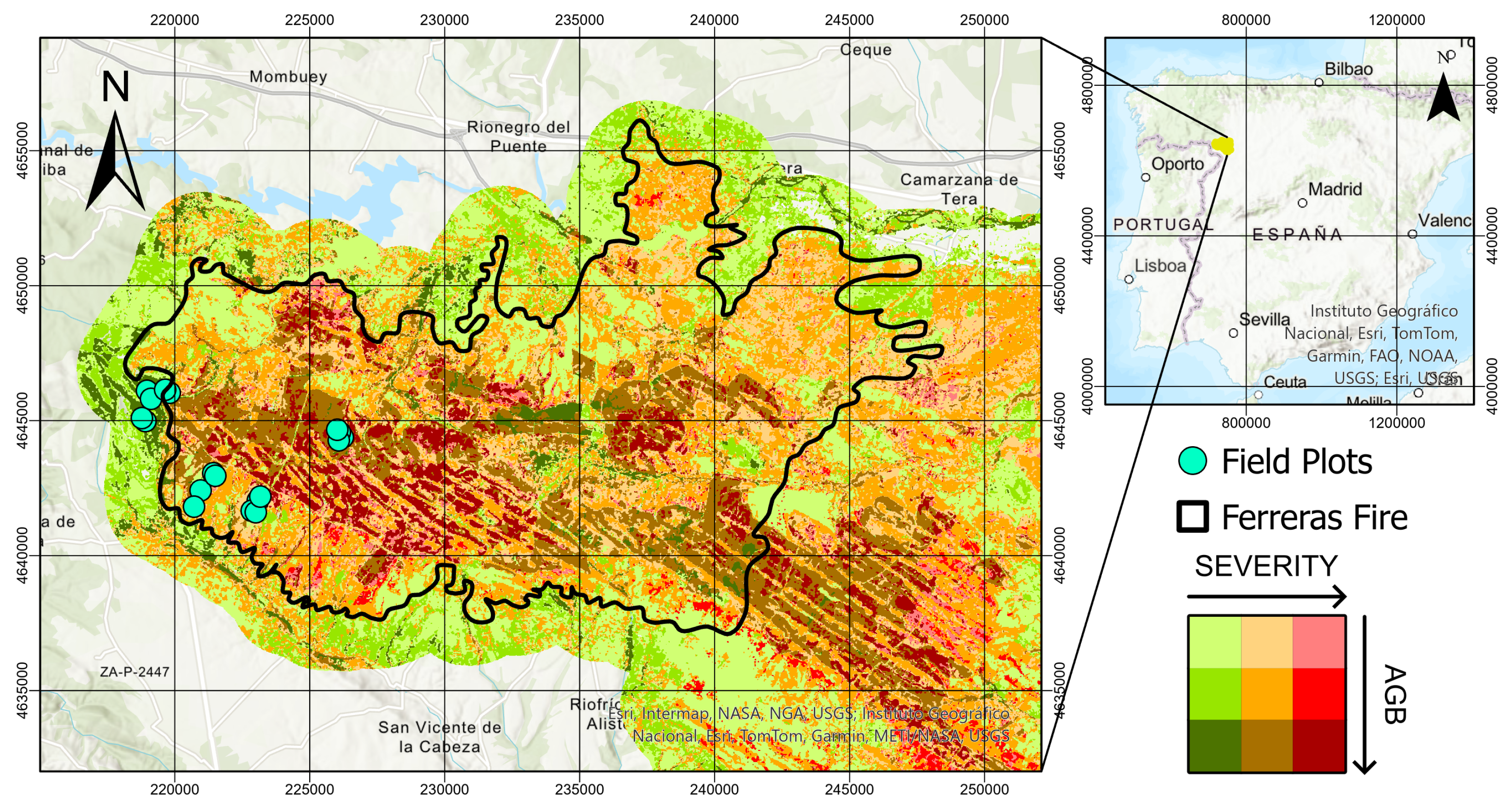
Two lightning-ignited wildfires started in June and July 2022, converging into a single burned patch affecting more than 50,000 ha (Figure 1). Severe drought conditions, a persistent heat wave, and strong and erratic winds, up to 70 km ${\mathrm{h}}^{-1}$, drove rapid fire spread. This study focuses on the first event, which began on 15 June 2022 and was extinguished on 24 June 2022, after burning 29,670 ha.

Figure 1. Sierra de la Culebra wildfire, showing burn severity and above-ground biomass (AGB) clustering. Unburned, moderately burned, and severely burned areas are shown in green, orange, and red. Darker tones indicate higher AGB density.

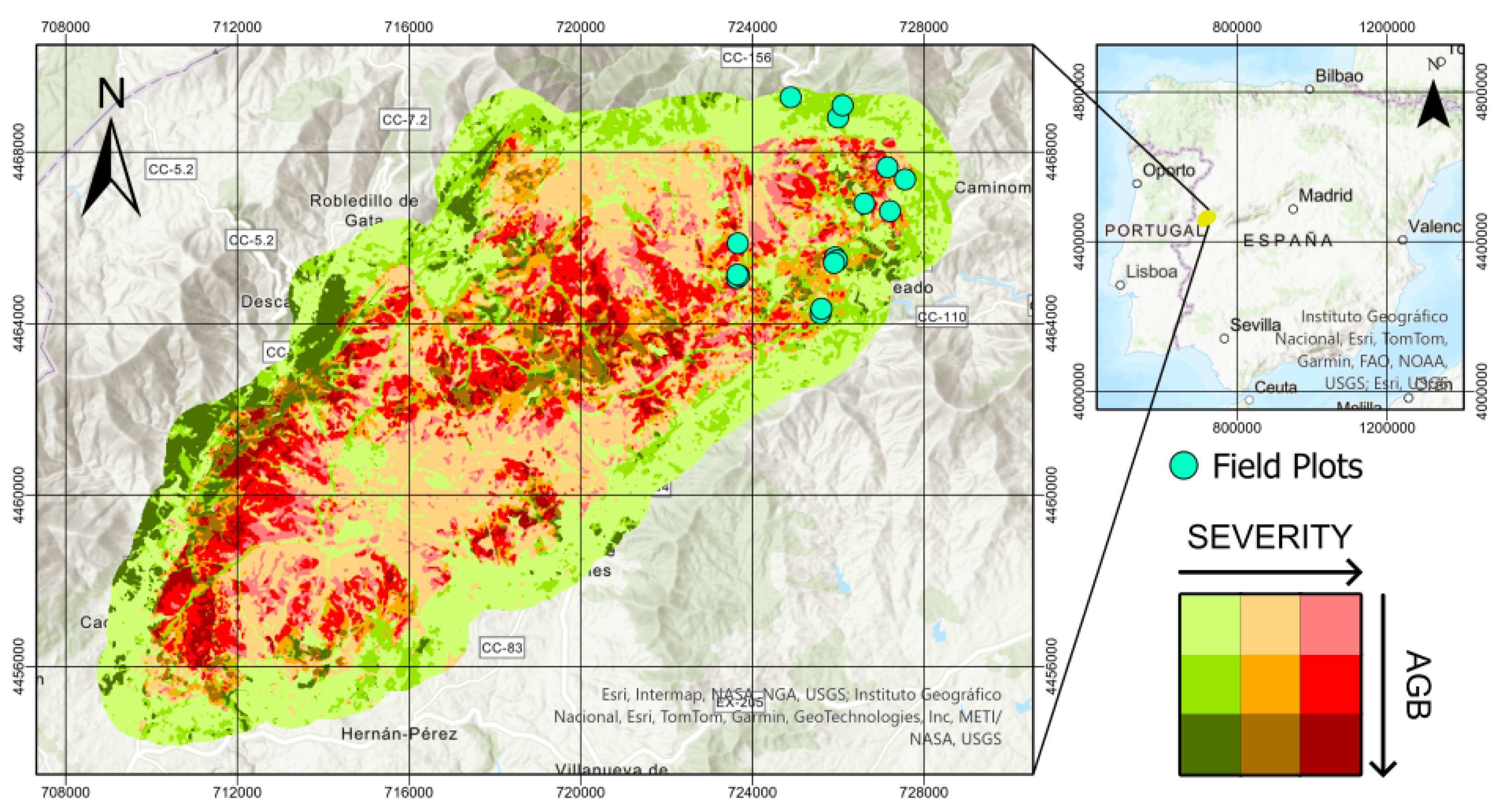
The Sierra de Gata is in northern Extremadura and has a Mediterranean climate (Csa) with a mean annual temperature of 12.5–15 °C and precipitation of 800–1000 mm [27]. The dominant trees are Quercus ilex, Eucalyptus camaldulensis, and Pinus pinaster; shrub species are mainly composed of Cistus ladanifer and Erica sp. [28]. The Pinofranqueado fire was intentionally ignited on 17 May 2023, under dry-storm conditions and winds of up to 50 km ${\mathrm{h}}^{-1}$, burning 10,863 ha (Figure 2), more than 97% of which were forests [29].

Figure 2. Sierra de Gata wildfire, showing burn severity and above-ground biomass (AGB) clustering. Unburned, moderately burned, and severely burned areas are shown in green, orange, and red. Darker tones indicate higher AGB density.

A summary of the main characteristics of the two study sites and the associated field and TLS datasets is provided in Table 1.

Table 1. Summary of the study sites and datasets used in this study.

Characteristic	S. Culebra	S. Gata
Wildfire year	2022	2023
Campaign dates	3–5 May 2023	9–13 September 2024
Ignition	Lightning	Intentional
Burned area (ha)	29,670	10,863
Climate (Köppen)	Csb	Csa
Dominant tree species	Pinus sylvestris, Pinus pinea	Pinus pinaster, Quercus ilex
No. plots (radius)	18 plots (15 m)	16 plots (17 m; ≈907 ${\mathrm{m}}^2$)
Field measurements	DBH and height	DBH, height and GPS location
Structural classification	PNOA airborne LiDAR K-means
Burn classification	Sentinel-2 dNBR Thresholding
Burn-severity classes	Unburned, moderate, and severe
TLS instrument	Leica RTC360 (Leica Geosystems AG, Heerbrugg, Switzerland)
Scan design	One central and four peripheral scans
Registration	Four spherical targets (12 cm)

2.2. Sampling Design

Two field campaigns were carried out to evaluate the performance of terrestrial LiDAR (TLS) for diameter at breast height (DBH) and above-ground biomass (AGB) retrieval under contrasting post-fire conditions. Plot locations were selected following a stratified random sampling design based on Homogeneous Response Areas (HRA), defined as zones having similar pre-fire structure within the same burn severity. Each HRA allows field measurements collected at the plot level to be interpreted as representative of broader areas, facilitating spatial extrapolation [30].

Pre-fire forest structure for both study areas was characterized using the Spanish National Aerial Orthophotography Plan (PNOA) airborne LiDAR dataset. A K-means clustering algorithm classified each site into three structural classes. The clustering was based on maximum return height (Hmax), mean return height (Hmean), the standard deviation of the height (Hstd), used as a proxy for vertical structural heterogeneity. In addition, fractional cover (FC) and the area under the canopy curve (AUC) were included as proxies for above-ground biomass [31].

Burn severity was classified using the differenced Normalized Burn Ratio (dNBR) from Sentinel-2 imagery. The threshold values were based on the ranges proposed by the USGS, but considering three categories: unburned (<0.1), low-moderate (0.1–0.44) and moderate-high (>0.44). Overlaying both classifications, we produced nine strata combining structure and severity classes.

For the Sierra de la Culebra study area, the field campaign was carried out from 3 to 5 May 2023. A total of 18 circular plots with a radius of 15 m were established across the selected strata. The three structural classes were:

1.

Low vegetation areas, characterized by fractional cover below 10%, mean height below 4 m, and low height variability.

2.

Open forest stands, with fractional cover below 30% and intermediate canopy heights (Hmean ≈ 5 m).

3.

Closed forest stands, showing fractional cover above 60% and higher mean heights (Hmean ≈ 10 m) with increased vertical heterogeneity.

Plots belonging to the first structural class were excluded from further analysis, as they predominantly represented shrub-dominated areas where tree-level DBH and biomass estimation were not applicable to the objectives of this study.

For the Pinofranqueado–Sierra de Gata study area, the field campaign took place from 9 to 13 September 2024. Sixteen circular plots with a radius of 17 m were established, corresponding to an area of approximately 907 ${\mathrm{m}}^2$, equivalent to the spatial resolution of a Landsat pixel. The derived structural classes were:

1.

Sparse young stands with low fractional cover and limited vertical development, FC < 35.2%, Hmean < 1.8 m, Hstd < 1.3 m.

2.

Young closed forests with intermediate canopy height and moderate structural variability, FC < 56%, Hmean ≈ 4.9 m, Hstd < 1.9 m.

3.

Closed forest stands characterized by high fractional cover and tall canopies with pronounced vertical heterogeneity, FC > 59%, Hmean ≈ 10.2 m, Hstd > 2.9 m.

Although plot radii differed between sites, this inconsistency has limited impact on the analysis: DBH was validated at the individual tree level, and the tree biomass was aggregated at the plot level to provide biomass density (Mg/ha).

The distribution of the plots according to their structural and burn severity properties is shown in Table 2.

Table 2. Distribution of plots by burn severity and structural class.

Burn Severity	Structural Class	Plots-S. Culebra	Plots-S. Gata
Unburned	Class 2	2	0
Unburned	Class 3	4	2
Moderate	Class 2	2	4
Moderate	Class 3	3	4
Severe	Class 2	3	2
Severe	Class 3	4	4

2.3. Field Inventory

For both sites, field measurements were collected simultaneously with TLS scans. The diameter at breast height (DBH) of all trees with DBH >7.5 cm was measured as the mean of two perpendicular axes at a height of 1.30 m using a calliper. Tree height was recorded for 25% of individuals using a Haglöf Vertex V (Haglöf Sweden AB, Långsele, Sweden). Species and number of trees were noted for each plot.

Additionally, for the Pinofranqueado-Sierra de Gata site, trees were located using a GPS with centimeter-level accuracy. In five of the plots, all trees were geolocated. In the remaining plots, we geolocated a sample of 20 trees, selected to represent the observed spatial and DBH distribution. These data were used to validate the accuracy of DBH estimation.

2.4. TLS Acquisition

TLS data was collected using a Leica RTC360 instrument operating in high resolution mode. The main technical specifications of the instrument are summarized in Table 3. Following the methodology proposed by other studies [32,33], each plot was scanned from five positions, one central and four at 7.5–8.5 m in the cardinal directions. The multi-scan configuration was designed to increase trunk visibility and reduce shadowing effects caused by trunks and remaining understory elements. This geometry is particularly important in post-fire conditions, where uneven char patterns can lead to spatially heterogeneous return intensity and point density. Using consistent scan geometry across plots also supports comparability between burn-severity classes, as differences in trunk coverage are less likely to arise from acquisition design.

Table 3. Technical specifications of the terrestrial laser scanner used in this study.

Specification	Leica RTC360
Laser class	Class 1
Ranging principle	Time-of-flight
Wavelength	1550 nm (SWIR)
Field of view (°)	360 (horizontal) × 300 (vertical)
Maximum range	65 m (High Res.)
Range accuracy	1.0 mm
Angular accuracy	0.087 mrad
Maximum measurement rate	Up to 2 million points ${\mathrm{s}}^{-1}$
Point spacing	≈3 mm at 10 m distance (High Res.)
Beam divergence	≈0.23 mrad
Number of returns	Single

Four 12 cm spherical targets were placed so that each scan observed at least three of them, ensuring accurate coregistration (target position error < 0.1 m; cloud-to-cloud error < 0.02 m). During the Sierra de la Culebra campaign, some light rain occurred, and the scanning was paused during rainfall to prevent intensity attenuation [34].

2.5. Data Processing

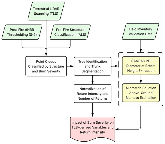
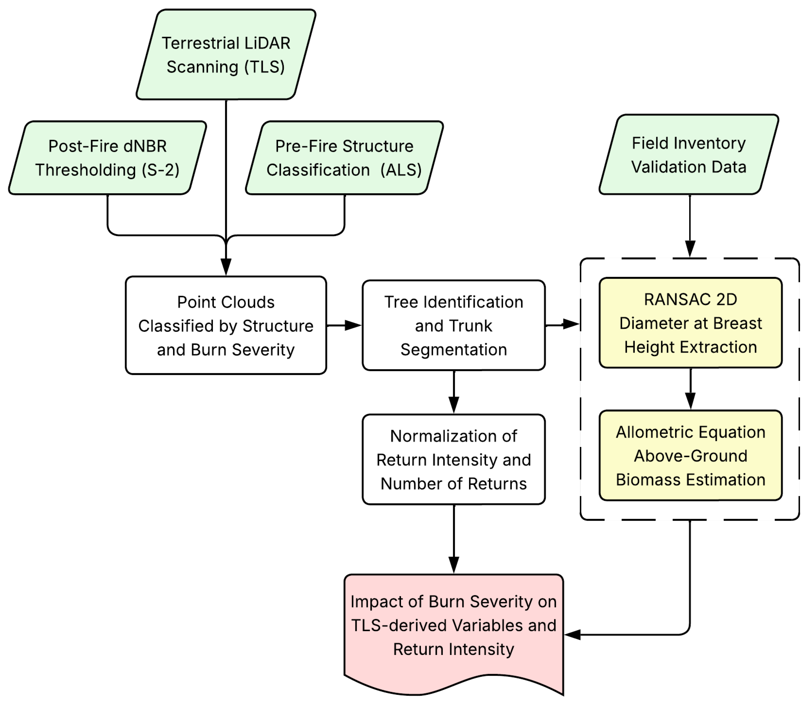
Figure 3 provides an overview of the methodological workflow adopted in this study. Each processing step and analysis component is described in detail in the following sections.

Figure 3. Overview of the methodological workflow.

Each plot contained approximately 250 million points (10 GB). Data was spatially indexed using the Lax extension [35] (LAStools version 171231, Rapidlasso GmbH, Gilching, Germany). Ground was classified using the Progressive Morphological Filter [36]. Height was normalized using a 0.10 m TIN Digital Terrain Model (DTM) as the ground surface. Ground points were removed, and Statistical Outlier Removal (SOR) was applied.

2.5.1. Segmentation and DBH Extraction

Individual trees were segmented from the normalized cloud using the Python 3.11 package TreeIso (accessed January 2025) [37]. We evaluated how burn severity impacted the number of returns for each tree and their intensity, since it can affect tree segmentation. We compared the mean intensity of the returns for each severity class and the number of returns relative to the unburned plots. Point features were calculated to filter out the understory and improve tree identification [21,38,39].

Following Zhou et al. [21], a set of twelve 2D and 3D geometric point features were extracted from the TLS point cloud to support tree segmentation and trunk identification. These features are derived from the eigenvalues of local covariance matrices and from neighborhood-based geometric properties. A summary of the extracted features and their definitions is provided in Table 4.

Table 4. Geometric point features extracted from the TLS point cloud for tree segmentation.

Point Feature	Definition
Linearity (3D)	Ratio of the largest eigenvalue to the sum of eigenvalues of the 3D local covariance matrix.
Planarity (3D)	Ratio of the intermediate eigenvalue to the sum of eigenvalues of the 3D local covariance matrix.
Omnivariance (3D)	Cubic root of the product of the three eigenvalues of the 3D local covariance matrix.
Anisotropy (3D)	Normalized difference between the largest and smallest eigenvalues of the 3D covariance matrix.
Verticality (3D)	Absolute vertical component of the normal vector estimated from the 3D neighborhood.
Radius (3D)	Mean distance of neighboring points to the local centroid in 3D space.
Density (3D)	Number of points within the defined 3D neighborhood.
Z-difference (3D)	Elevation range within the 3D local neighborhood.
Z-standard deviation (3D)	Standard deviation of point elevations within the 3D neighborhood.
Radius (2D)	Mean distance of neighboring points to the local centroid projected onto the horizontal plane.
Density (2D)	Number of points within the defined 2D neighborhood.
Linearity (2D)	Ratio of the largest eigenvalue to the sum of eigenvalues of the 2D local covariance matrix.

Segmentation followed an iterative implementation of TreeIso. Initial parameters $(K_1,{\Lambda }_1,K_2,{\Lambda }_2)$ were applied, and each cluster was visually inspected. Segments corresponding to individual trees were extracted, while merged groups were reprocessed with reduced $K_1$ and $K_2$, causing further splitting. Trunk isolation was high (≈85–90%) but exhibited partial crown loss. Subsequently, segmented trees were sliced at 1.25–1.35 m and projected onto the XY-plane. DBH was extracted by applying a 2D RANSAC circle fitting algorithm [40,41]:

$$x_i^2+y_i^2+2h{x}_i+2k{y}_i+c=0$$

(1)

where $(-h,-k)$ is the center and $r^2=h^2+k^2-c$ gives the radius. Points within threshold $ϵ$ of the circle were considered inliers, selecting the circle with the most inliers after T trials. The parameters $ϵ=0.015$ m and $T=34$ followed the values reported by [40] and were verified to ensure an adequate fit with our data.

2.5.2. Impact of Burn Severity on DBH Extraction

To evaluate the effect of burn severity on DBH extraction, we first need to quantify the area of the trunk seen by the scans. The scanner cannot observe the full circumference, and each scan samples a different portion of the trunk. Even with multiple scan positions intended to minimize occlusion, trunks are not covered uniformly. Therefore, we seek to determine which parts of the 1.25–1.35 m slice (from which DBH is extracted) are visible, and to normalize return counts by the scanned trunk area. Thus, the cylindrical surface was unwrapped into 36 angular sectors.

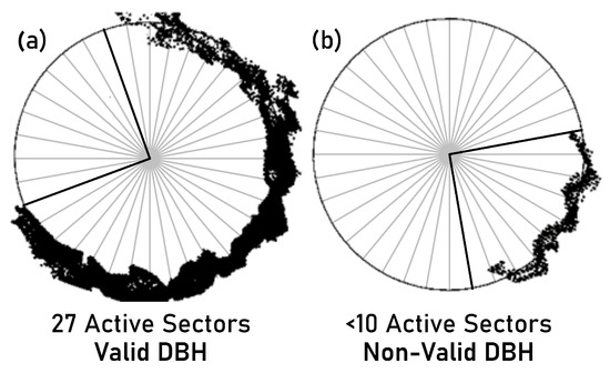
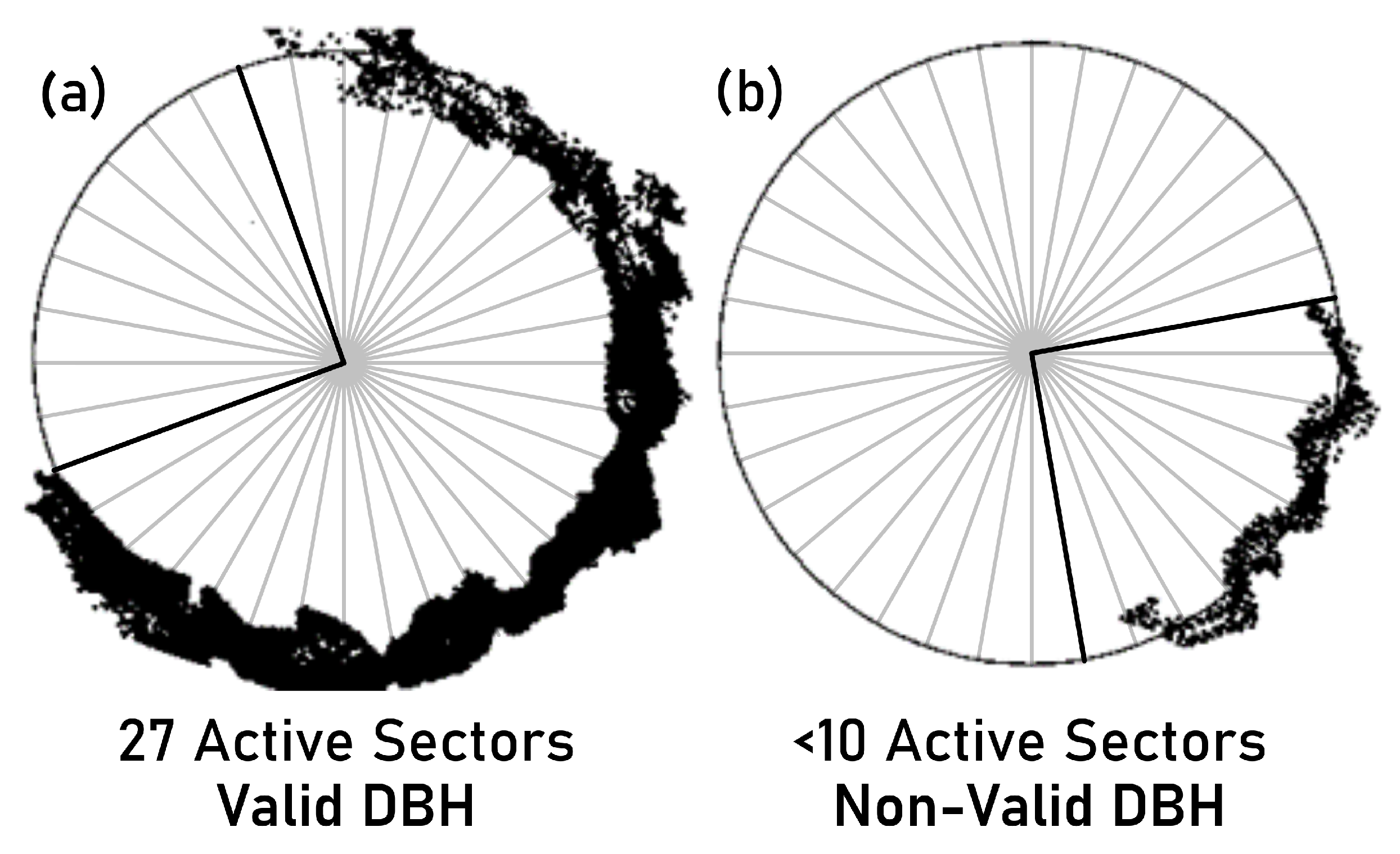
The RANSAC algorithm requires at least three non-collinear points to fit a circle. However, such minimal configurations are unstable for TLS trunks. In this study, slices containing fewer than 50 points or showing less than 25% trunk coverage (<10 active angular sectors; Figure 4) were considered non-valid DBHs, as RANSAC fitting becomes unreliable under sparse or uneven point distributions [42,43].

Figure 4. Transversal trunk section illustrating the angular sector approach used to evaluate trunk coverage for DBH extraction. The trunk slice is unwrapped into 36 angular sectors. (a) Example of a well-sampled trunk section with sufficient angular coverage (27 active sectors). (b) Example of a sparsely sampled trunk section with fewer than 10 active sectors, leading to an unreliable circle fit and a non-valid DBH.

For each trunk, we extracted TLS return counts ($R_i$) and mean intensity from the 1.25–1.35 m slice. Sectors with zero returns were excluded. The scanned area and normalized return density were computed using Equation (2):

$$A_i=t2\pi r_i{\displaystyle \frac{s_i}{36}},D_i={\displaystyle \frac{R_i}{0.10\times 2\pi r_i\times (s_i/36)}}$$

(2)

where $t=0.10$ m and $s_i$ is the number of active sectors.

The effect of burn severity on return intensity and number of returns was assessed using Spearman correlations, given the non-normal distribution of intensity values across plots. Spearman’s $\rho$ was computed between return intensity and both AGB estimation accuracy and normalized number of returns, with significance tested at the reported p-values.

2.5.3. Above-Ground Biomass Estimation

AGB was estimated for each tree using the allometric equations proposed by [44], which used the following form:

$$\mathrm{AGB}=\mathrm{CF}\times a\times {\mathrm{DBH}}^b$$

(3)

where CF corrects for log-transformation bias, and a and b are species-specific parameters. Ref. [44] provided parameters for different biomass fractions of the tree, including total biomass, trunk, branches > 7 cm, branches between 2–7 cm and branches < 2 cm and foliage. Plot level biomass was obtained by summing up the biomass of the trees within each plot and subsequently converted to biomass density (Mg ${\mathrm{h}\mathrm{a}}^{-1}$).

Because Equation (3) applies only to healthy individuals, and the biomass of burned plots had been partially consumed, we visually estimated biomass consumption by quadrants (NW, NE, SW, SE) following other studies [45,46]. At least two experts independently estimated consumed fractions for trunk, large branches (>7 cm), medium branches (2–7 cm), and small branches + foliage (<2 cm). When independent estimates were in close agreement, the mean value was used as the final estimate. In cases of substantial discrepancy, the two raters discussed until reaching a consensus value.

Validation of DBH and AGB estimates was performed at the individual and plot level, respectively. A total of 23 plots were used for AGB estimation (8 unburned, 7 moderately burned, 8 severely burned). For DBH validation, 807 trees, including 165 unburned, 437 moderately burned, and 205 severely burned, measured in 34 plots were used. The effect of burn severity on intensity and number of returns was evaluated using the 437 moderately burned and 205 severely burned trees. TLS and field trees were matched using centimeter-level GPS with a maximum offset of 0.15 m. Trees with DBH <7.5 cm were excluded since they were not measured in the field. AGB and DBH estimates were evaluated using overall accuracy (OA), root mean square error (RMSE), and relative RMSE (rRMSE).

The unequal distribution of plots across severity classes reflects logistical constraints during field campaigns, including terrain difficulty and plot accessibility, rather than a sampling design decision. Nevertheless, accuracy metrics were computed independently per severity class to avoid bias.

3. Results

3.1. Return Intensity and Number of Returns

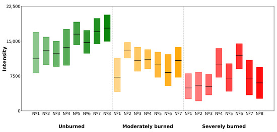
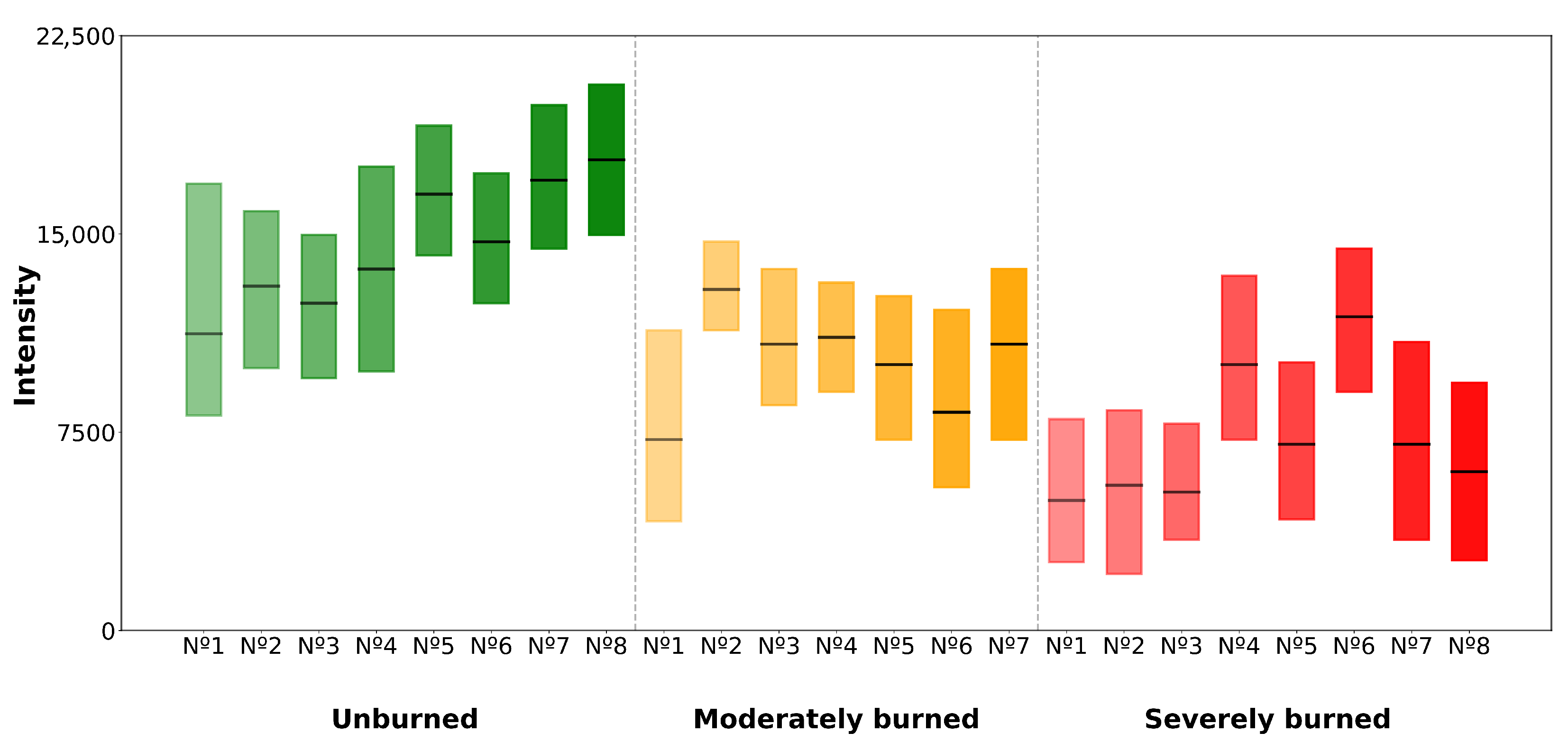
Return intensity decreased with burn severity (Figure 5). Mean intensity was $14,544(\pm 2373)$ for unburned plots, $10,171(\pm 1895)$ for moderately burned, and 7210 (±2489) for severely burned plots. Relative to unburned plots, on average, moderately burned plots retained only 85.1% of the returns per unit trunk area, and severely burned plots retained 45.7% per unit trunk area. Return intensity was strongly correlated with both AGB estimation accuracy ($\rho =0.72$, $p<0.001$) and normalized number of returns ($\rho =0.85$, $p<0.000001$).

Figure 5. Return intensity by burn severity at 1.25–1.35 m trunk height. The central line within each box represents the median value. Unburned, moderately burned, and severely burned areas are shown in green, orange, and red.

The number of trees segmented by TLS relative to field data, and the proportion of segmented trees that provided valid slices for DBH estimation, are summarized in Table 5. Segmentation identified on average $85.0\%(\pm 13.22\%)$ of reference trees in unburned plots, $92.5\%(\pm 6.45\%)$ in moderately burned, and $87.0\%(\pm 5.50\%)$ in severely burned plots. Valid DBHs represented $92.13\%\pm 1.30\%$ and $93.46\%\pm 7.73\%$ of segmented trees in unburned and moderate plots, but dropped to $73.58\%\pm 12.72\%$ in severe plots.

Table 5. Segmented trees relative to field data and proportion with valid DBH slices across burn-severity levels.

Severity	Segmented Trees (%)	Segmented with Valid DBH Slice (%)
Unburned	$85.0\pm 13.22$	$92.13\pm 1.30$
Moderate	$92.5\pm 6.45$	$93.46\pm 7.73$
Severe	$87.0\pm 5.50$	$73.58\pm 12.72$

3.2. DBH Estimation

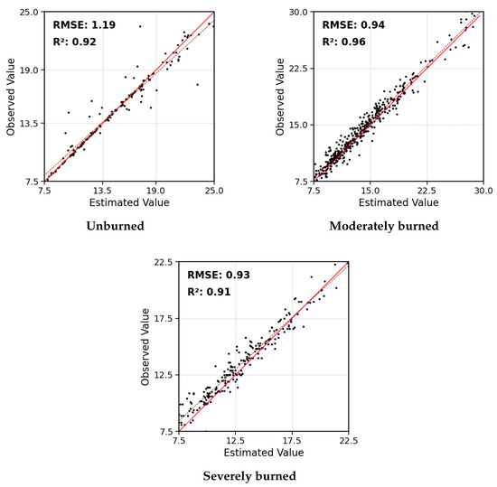
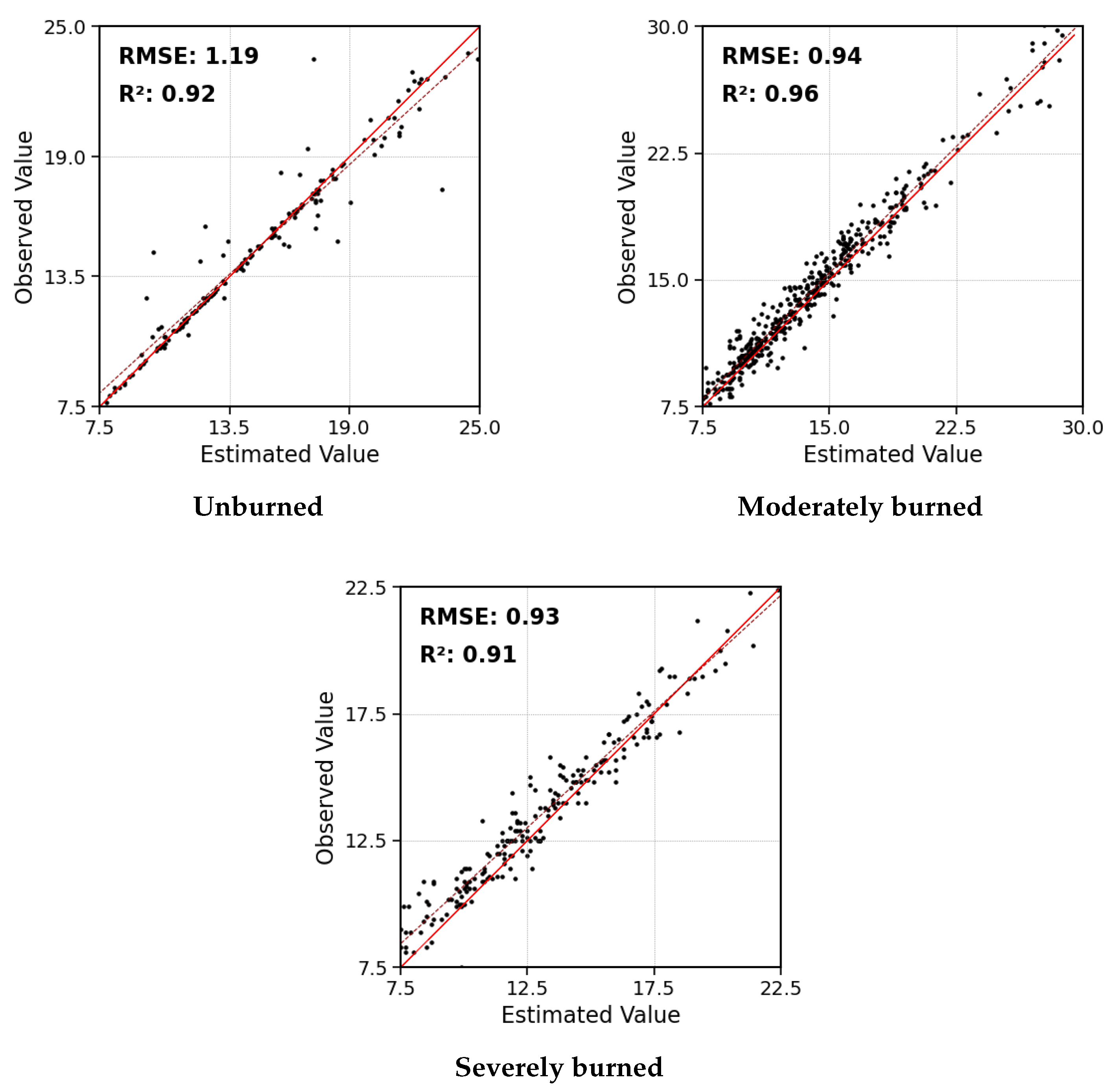
Diameter at breast height (DBH) was validated at the tree level. TLS-derived DBH values showed strong agreement with field measurements across all fire-severity classes (Figure 6).

Figure 6. Scatterplots of TLS-derived vs. field-measured DBH for unburned, moderately burned, and severely burned trees. The dashed red line represents the 1:1 relationship and the solid red line represents the linear regression fit.

For unburned trees, TLS-derived DBH showed a strong agreement with field data ($R^2=0.92$, RMSE = 1.19 cm, rRMSE = 7.97%). Accuracy increased slightly in moderately burned plots ($R^2=0.96$, RMSE = 0.94 cm, rRMSE = 6.46%). Severely burned trees maintained comparable precision ($R^2=0.91$, RMSE = 0.93 cm, rRMSE = 6.94%).

3.3. AGB Estimation

Accuracy decreased with burn severity, with TLS-derived values representing 93%, 88%, and 74% of reference biomass for unburned, moderately burned, and severely burned plots, respectively (Table 6).

Table 6. TLS-derived AGB accuracy relative to field reference values across burn-severity levels.

Plot Number	Unburned	Moderate	Severe
Plot Number 1	83.3	65.1	35.3
Plot Number 2	89.9	91.9	69.7
Plot Number 3	90.4	92.5	73.4
Plot Number 4	94.9	94.5	97.2
Plot Number 5	99.7	95.3	56.2
Plot Number 6	91.1	86.8	94.8
Plot Number 7	98.0	89.2	91.4
Plot Number 8	97.6	–	77.9
Average	93.0 ± 5.4	87.9 ± 10.5	74.5 ± 21.1

Translated into Mg ${\mathrm{h}\mathrm{a}}^{-1}$, and adjusted for wildfire consumption, unburned plots averaged 76.3 (±33.2) Mg ${\mathrm{h}\mathrm{a}}^{-1}$ with MAE = 4.6 (±3.8) Mg ${\mathrm{h}\mathrm{a}}^{-1}$; moderately burned plots averaged 65.1 (±24.2) Mg ${\mathrm{h}\mathrm{a}}^{-1}$ with MAE = 6.4 (±2.8) Mg ${\mathrm{h}\mathrm{a}}^{-1}$; and severely burned plots showed the lowest biomass, 32.9 (±22.7) Mg ${\mathrm{h}\mathrm{a}}^{-1}$, and MAE = 6.1 (±4.0) Mg ${\mathrm{h}\mathrm{a}}^{-1}$.

Species-specific equations introduced minor variability. Table 7 shows the biomass obtained for a tree with the average DBH from our unburned plots, DBH ≈ 15 cm using four different species-specific formulas from Montero et al. [44]. The resulting biomass varied between 43.47 kg and 73.49 kg depending on the species.

Table 7. Species-specific equations from Montero et al. [44] and resulting AGB estimates for DBH = 15 cm.

Species	Equation	AGB (kg)
Pinus pinaster	$exp({0.173491}^2/2)·exp(-3.00347)·{DBH}^{2.49641}$	43.47
Pinus sylvestris	$exp({0.246887}^2/2)·exp(-2.50275)·{DBH}^{2.41194}$	57.93
Quercus pyrenaica	$exp({0.247318}^2/2)·exp(-2.59695)·{DBH}^{2.53453}$	73.49
Quercus faginea	$exp({0.170157}^2/2)·exp(-2.89305)·{DBH}^{2.52426}$	52.31

To estimate the contribution of the absence of species identification at the tree level to total AGB error, plot-level AGB was computed twice for each plot: once using the field-recorded species-specific equation for each individual tree, and once using only the dominant species equation applied to all trees, as is necessarily done when processing our TLS data without species labels. The difference between these two estimates accounted for an average of 4.76%, 3.83%, and 2.06% of plot-level AGB in unburned, moderately burned, and severely burned plots, respectively, reflecting the sensitivity to species assignment under the species composition observed in each plot.

Regarding the effect of burn severity on AGB estimation, AGB errors increased with burn severity, primarily due to the reduction in return intensity and the lower number of usable DBHs. These factors reduced the number of trunks contributing valid DBH estimates, which propagated into plot-level biomass uncertainty.

4. Discussion

4.1. Return Intensity and Number of Returns

Return intensity depends on multiple factors, including range, incidence angle, surface roughness, and target reflectance [47]. During a wildfire, wood pyrolysis forms a superficial char layer on bark and sapwood, reducing reflectance in the SWIR region used by the RTC360 system (1550 nm), which is a key factor influencing return intensity [48]. In severely burned plots, charring extended beyond 2 m, completely covering the height at which DBH is extracted (1.25–1.35 m), significantly reducing return intensity. Moreover, the instrument’s wavelength is highly sensitive to surface moisture [49]. Mild rainfall occurred during TLS acquisition in Sierra de la Culebra, and the high porosity of charred wood can enhance water absorption [50], further reducing effective reflectance.

Our results suggest that TLS measurements are relatively resistant to moderate reductions in return intensity found on moderately burned plots, but estimation performance declines sharply in high severity plots due to the significantly lower intensity of the returns recorded by the sensor. The decline from 14,544 units of intensity in unburned plots to 10,171 in moderately burned plots only prompted a slight reduction in the number of returns collected (14.9%), while the further loss of ≈3000 units of intensity in severely burned plots (7210) represented a much steeper 54.3% reduction, which translated into a lower percentage of segmented trees and usable DBH slices, reducing the overall AGB accuracy at the plot level.

4.2. Estimation of DBH

TLS-derived DBH achieved high accuracy across burn severities (overall accuracy = 94.5%, MAE = 0.78 cm, RMSE = 1.02 cm). These results align with previous studies using high-resolution TLS for tree-level measurements, such as [51], who reported MAE = 0.92 cm and RMSE = 1.8 cm. Although charring alters the bark surface texture, fire consumption in the Mediterranean pine ecosystem is concentrated in foliage and fine fuel fraction [52], leaving trunk geometry mostly intact. Field-measure DBH is therefore not meaningfully affected, remaining as a reliable reference for validation.

Relative errors were consistent among severity classes (rRMSE = 7.97% unburned; 6.46% moderate; 6.94% severe). In unburned plots, understory vegetation and low branches that were not fully removed during preprocessing partially interfere with trunk isolation during segmentation, introducing errors in the trunk slice from which DBH is extracted. Fire removes these elements in burned plots, improving trunk isolation and partially explaining the slightly lower errors observed under moderate and severe conditions. The use of a robust circle-fitting algorithm (RANSAC 2D) improved DBH stability under incomplete or noisy point distributions, confirming previous findings on its reliability for forest trunks [40,53]. This robustness was particularly valuable in burned plots, where return intensity and point density were substantially reduced, ensuring consistent DBH extraction despite data degradation.

4.3. Estimation of AGB

Errors in AGB estimation originated from DBH uncertainty and errors in species identification since the allometric model used was based on DBH and species-specific parameters. Despite the fact that tree species identification from LiDAR metrics can exceed 90% accuracy in unburned forests [54], species identification was not attempted in post-fire conditions, as fire alters bark texture and crown architecture, eliminating the structure on which classification approaches rely in undisturbed forests. Species were therefore assigned based on the dominant species recorded during the field campaigns.

The use of allometric equations based on DBH and height can improve the estimation of AGB [55]. However, metrics such as tree height, return intensity, crown volume, and crown base height [56,57,58] could be altered by the wildfire, particularly in high burn severity patches, propagating uncertainty into AGB estimates.

AGB accuracy declined with severity, from 93% in unburned to 88% in moderately burned and 74% in severely burned plots. This reduction in accuracy is consistent with the propagation of DBH errors into allometric models.

In moderately burned plots, accuracy loss can be largely attributed to the absence of species identification, as point density and segmentation performance remained high. It is expected that this error increases with the number of species present in the plot.

In severely burned plots, in addition to errors in species identification, intensity and return loss became the dominant source of error. These plots lost 54.3% of the returns compared to the unburned stands, reducing usable DBHs from 92% to 74%. Consequently, the average density of biomass estimated (32.90 Mg ${\mathrm{h}\mathrm{a}}^{-1}$) was considerably lower than the average density observed (44.16 Mg ${\mathrm{h}\mathrm{a}}^{-1}$).

4.4. Limitations

Several limitations should be considered when interpreting these results. TLS campaigns were conducted 11 and 16 months after the respective fire events, to evaluate post-fire vegetation recovery. At both sites, trunk surfaces at DBH extraction height (1.25–1.35 m) were bare and charred in burned plots, with only sparse, sapling regrowth observed.

Visual estimation of biomass consumption is inherently subjective. However, the use of at least two independent raters, combined with a quadrant-level protocol following established field practice [45,46], limits the impact of individual judgment.

The uncertainty introduced by the lack of species assignment was small relative to the errors generated by severe intensity-driven return loss, but would increase in mixed stands with greater diversity.

Finally, it is worth mentioning that the instrument Leica RTC360 operates as a single return instrument, recording only one return per pulse. In severely charred trunks, the single return may fall below the detection threshold entirely. Multi-return systems might be able to partially recover from signal loss.

5. Conclusions

This study assessed the influence of burn severity on TLS-based estimations of forest structure variables. The DBH was accurately retrieved, with no significant decrease in accuracy with higher severity (mean accuracy = 94.5%, RMSE = 1.02 cm).

The AGB errors propagated mainly from the DBH uncertainties, which were amplified under severe burning by the loss of return intensity and point density. These factors did not significantly limit tree segmentation but reduced the number of usable DBHs, lowering plot-level AGB accuracy from 93.0% in unburned plots to 74.5% in severely burned plots. Return intensity proved critical for reliable measurements, as trunk charring and moisture-induced absorption reduced effective reflectance in the SWIR wavelength. AGB accuracy was further reduced by the impossibility of correctly identifying the species of the segmented trees.

The evaluation framework presented here is applicable to other forested ecosystems affected by fire. Our results support caution when interpreting plot level estimates derived from TLS in high-severity fire conditions, however, this effect may vary depending on the emission wavelength and power of the instrument used.

Overall, TLS proved reliable for post-fire forest inventory in low-to-moderate severity conditions, where DBH extraction and biomass estimation remained accurate. In high-severity areas, return loss induced by scorched trunks limited tree detectability and reduced plot-level AGB, highlighting the need for methods and acquisition protocols robust to low-intensity returns.

References

- Ellison, D.; Morris, C.E.; Locatelli, B.; Sheil, D.; Cohen, J.; Murdiyarso, D.; Gutierrez, V.; van Noordwijk, M.; Creed, I.F.; Pokorny, J.; et al. Trees, forests and water: Cool insights for a hot world. Glob. Environ. Change 2017, 43, 51–61. [Google Scholar] [CrossRef] [Scilit]
- Psistaki, K.; Tsantopoulos, G.; Paschalidou, A.K. An Overview of the Role of Forests in Climate Change Mitigation. Sustainability 2024, 16, 6089. [Google Scholar] [CrossRef] [Scilit]
- Hämäläinen, A.; Runnel, K.; Ranius, T.; Strengbom, J. Diversity of forest structures important for biodiversity is determined by the combined effects of productivity, stand age, and management. Ambio 2024, 53, 718–729. [Google Scholar] [CrossRef] [Scilit]
- Toivonen, J.; Kangas, A.; Maltamo, M.; Kukkonen, M.; Packalen, P. Assessing biodiversity using forest structure indicators based on airborne laser scanning data. For. Ecol. Manag. 2023, 546, 121376. [Google Scholar] [CrossRef] [Scilit]
- Bispo, P.D.C.; Dos Santos, J.R.; Valeriano, M.D.M.; Graça, P.M.L.D.A.; Balzter, H.; França, H.; Bispo, P.D.C. Predictive models of primary tropical forest structure from geomorphometric variables based on SRTM in the Tapajo’s region, Brazilian Amazon. PLoS ONE 2016, 11, e0152009. [Google Scholar] [CrossRef] [Scilit]
- Reddington, C.L.; Morgan, W.T.; Darbyshire, E.; Brito, J.; Coe, H.; Artaxo, P.; Scott, C.E.; Marsham, J.; Spracklen, D.V. Biomass burning aerosol over the Amazon: Analysis of aircraft, surface and satellite observations using a global aerosol model. Atmos. Chem. Phys. 2019, 19, 9125–9152. [Google Scholar] [CrossRef] [Scilit]
- Buchholz, R.R.; Hammerling, D.; Worden, H.M.; Deeter, M.N.; Emmons, L.K.; Edwards, D.P.; Monks, S.A. Links Between Carbon Monoxide and Climate Indices for the Southern Hemisphere and Tropical Fire Regions. J. Geophys. Res. Atmos. 2018, 123, 9786–9800. [Google Scholar] [CrossRef] [Scilit]
- Gould, C.F.; Heft-Neal, S.; Johnson, M.; Aguilera, J.; Burke, M.; Nadeau, K. Health Effects of Wildfire Smoke Exposure. Annu. Rev. Med. 2024, 75, 277–292. [Google Scholar] [CrossRef] [Scilit] [PubMed]
- Hermesdorf, L.; Elberling, B.; D’Imperio, L.; Xu, W.; Lambæk, A.; Ambus, P.L. Effects of fire on CO2, CH4, and N2O exchange in a well-drained Arctic heath ecosystem. Global Change Biol. 2022, 28, 4882–4899. [Google Scholar] [CrossRef] [Scilit] [PubMed]
- Ruffault, J.; Curt, T.; Moron, V.; Trigo, R.M.; Mouillot, F.; Koutsias, N.; Pimont, F.; Martin-StPaul, N.; Barbero, R.; Dupuy, J.L.; et al. Increased likelihood of heat-induced large wildfires in the Mediterranean Basin. Sci. Rep. 2020, 10, 13790. [Google Scholar] [CrossRef] [Scilit] [PubMed]
- Kalabokidis, K.; Palaiologou, P.; Gerasopoulos, E.; Giannakopoulos, C.; Kostopoulou, E.; Zerefos, C. Effect of Climate Change Projections on Forest Fire Behavior and Values-at-Risk in Southwestern Greece. Forests 2015, 6, 2214. [Google Scholar] [CrossRef] [Scilit]
- Stephens, S.L.; Agee, J.K.; Fulé, P.Z.; North, M.P.; Romme, W.H.; Swetnam, T.W.; Turner, M.G. Managing Forests and Fire in Changing Climates. Science 2013, 342, 41–42. [Google Scholar] [CrossRef] [Scilit]
- Sagra, J.; Moya, D.; Plaza-Álvarez, P.A.; Lucas-Borja, M.E.; Alfaro-Sánchez, R.; De Las Heras, J.; Ferrandis, P. Predation on Early Recruitment in Mediterranean Forests after Prescribed Fires. Forests 2017, 8, 243. [Google Scholar] [CrossRef] [Scilit]
- D’hont, B.; Calders, K.; Bartholomeus, H.; Lau, A.; Terryn, L.; Verhelst, T.; Verbeeck, H. Evaluating airborne, mobile and terrestrial laser scanning for urban tree inventories: A case study in Ghent, Belgium. Urban For. Urban Green. 2024, 99, 128428. [Google Scholar] [CrossRef] [Scilit]
- Newnham, G.J.; Armston, J.D.; Calders, K.; Disney, M.I.; Lovell, J.L.; Schaaf, C.B.; Strahler, A.H.; Danson, F.M. Terrestrial laser scanning for plot-scale forest measurement. Curr. For. Rep. 2015, 1, 239–251. [Google Scholar] [CrossRef] [Scilit]
- Calders, K.; Adams, J.; Armston, J.; Bartholomeus, H.; Bauwens, S.; Bentley, L.P.; Chave, J.; Danson, F.M.; Demol, M.; Disney, M.; et al. Terrestrial laser scanning in forest ecology: Expanding the horizon. Remote Sens. Environ. 2020, 251, 112102. [Google Scholar] [CrossRef] [Scilit]
- Delagrange, S.; Jauvin, C.; Rochon, P. PypeTree: A Tool for Reconstructing Tree Perennial Tissues from Point Clouds. Sensors 2014, 14, 4271–4289. [Google Scholar] [CrossRef] [Scilit] [PubMed]
- Hackenberg, J.; Wassenberg, M.; Spiecker, H.; Sun, D. Non Destructive Method for Biomass Prediction Combining TLS Derived Tree Volume and Wood Density. Forests 2015, 6, 1274–1300. [Google Scholar] [CrossRef] [Scilit]
- Solares-Canal, A.; Alonso, L.; Picos, J.; Armesto, J. Automatic tree detection and attribute characterization using portable terrestrial lidar. Trees-Struct. Funct. 2023, 37, 963–979. [Google Scholar] [CrossRef] [Scilit]
- Zhao, K.; García, M.; Liu, S.; Guo, Q.; Chen, G.; Zhang, X.; Zhou, Y.; Meng, X. Terrestrial lidar remote sensing of forests: Maximum likelihood estimates of canopy profile, leaf area index, and leaf angle distribution. Agric. For. Meteorol. 2015, 209–210, 100–113. [Google Scholar] [CrossRef] [Scilit]
- Zhou, J.; Wei, H.; Zhou, G.; Song, L. Separating leaf andwood points in terrestrial laser scanning data using multiple optimal scales. Sensors 2019, 19, 1852. [Google Scholar] [CrossRef] [Scilit]
- Terryn, L.; Calders, K.; Åkerblom, M.; Bartholomeus, H.; Disney, M.; Levick, S.; Origo, N.; Raumonen, P.; Verbeeck, H. Analysing individual 3D tree structure using the R package ITSMe. Methods Ecol. Evol. 2023, 14, 231–241. [Google Scholar] [CrossRef] [Scilit]
- Rocha, K.D.; Silva, C.A.; Cosenza, D.N.; Mohan, M.; Klauberg, C.; Schlickmann, M.B.; Xia, J.; Leite, V.R.; Alves de Almeida, D.R.; Atkins, J.W.; et al. Crown-Level Structure and Fuel Load Characterization from Airborne and Terrestrial Laser Scanning in a Longleaf Pine (Pinus palustri Mill.) Forest Ecosystem. Remote Sens. 2023, 15, 1002. [Google Scholar] [CrossRef] [Scilit]
- Hudak, A.T.; Kato, A.; Bright, B.C.; Loudermilk, E.L.; Hawley, C.; Restaino, J.C.; Ottmar, R.D.; Prata, G.A.; Cabo, C.; Prichard, S.J.; et al. Towards Spatially Explicit Quantification of Pre- A nd Postfire Fuels and Fuel Consumption from Traditional and Point Cloud Measurements. For. Sci. 2020, 66, 428–442. [Google Scholar] [CrossRef] [Scilit]
- Fernández-Guisuraga, J.M.; Suárez-Seoane, S.; Fernandes, P.M.; Fernández-García, V.; Fernández-Manso, A.; Quintano, C.; Calvo, L. Pre-fire aboveground biomass, estimated from LiDAR, spectral and field inventory data, as a major driver of burn severity in maritime pine (Pinus pinaster) ecosystems. For. Ecosyst. 2022, 9, 100022. [Google Scholar] [CrossRef] [Scilit]
- Pascual, A.; Guerra-Hernández, J. An integrated assessment of carbon emissions from forest fires beyond impacts on aboveground biomass. A showcase using airborne lidar and GEDI data over a megafire in Spain. J. Environ. Manag. 2023, 345, 118709. [Google Scholar] [CrossRef] [Scilit]
- Chazarra Bernabé, A.; Flórez García, E.; Peraza Sánchez, B.; Tohá Rebull, T.; Lorenzo Mariño, B.; Criado Pinto, E.; Moreno García, J.V.; Romero Fresneda, R.; Botey Fullat, R. Mapas Climáticos de España (1981–2010), AEMET., n.d. Available online: https://www.aemet.es/es/serviciosclimaticos/datosclimatologicos/valoresclimatologicos (accessed on 1 March 2025).
- MITECO. Cuarto Inventario Foreatal Nacional (MITECO); MITECO: Madrid, Spain, 2008.
- EEA. Corine Land Cover 2018 (CLC2018). 2019. Available online: https://sdi.eea.europa.eu/catalogue/copernicus/api/records/71c95a07-e296-44fc-b22b-415f42acfdf0?language=all (accessed on 20 October 2024).
- Chávez-Durán, Á.A.; Olvera-Vargas, M.; Figueroa-Rangel, B.; García, M.; Aguado, I.; Ruiz-Corral, J.A. Mapping Homogeneous Response Areas for Forest Fuel Management Using Geospatial Data, K-Means, and Random Forest Classification. Forests 2022, 13, 1970. [Google Scholar] [CrossRef] [Scilit]
- Huesca, M.; Roth, K.L.; García, M.; Ustin, S.L. Discrimination of Canopy Structural Types in the Sierra Nevada Mountains in Central California. Remote Sens. 2019, 11, 1100. [Google Scholar] [CrossRef] [Scilit]
- Béland, M.; Kobayashi, H. Mapping forest leaf area density from multiview terrestrial lidar. Methods Ecol. Evol. 2021, 12, 619–633. [Google Scholar] [CrossRef] [Scilit]
- Guo, X.; Wang, L.; Tian, J.; Yin, D.; Shi, C.; Nie, S. Vegetation horizontal occlusion index (VHOI) from TLS and UAV image to better measure mangrove LAI. Remote Sens. 2018, 10, 1739. [Google Scholar] [CrossRef] [Scilit]
- Fersch, T.; Buhmann, A.; Koelpin, A.; Weigel, R. The influence of rain on small aperture LiDAR sensors. In Proceedings of the 2016 German Microwave Conference (GeMiC); IEEE: Piscataway, NJ, USA, 2016; pp. 84–87. [Google Scholar] [CrossRef] [Scilit]
- Isenburg, M. LASindex–Spatial Indexing of LiDAR Data. 2012. Available online: https://rapidlasso.de/lasindex-spatial-indexing-of-lidar-data/ (accessed on 13 September 2024).
- Zhang, K.; Chen, S.C.; Whitman, D.; Shyu, M.L.; Yan, J.; Zhang, C. A progressive morphological filter for removing nonground measurements from airborne LIDAR data. IEEE Trans. Geosci. Remote Sens. 2003, 41, 872–882. [Google Scholar] [CrossRef] [Scilit]
- Xi, Z.; Hopkinson, C. 3D Graph-Based Individual-Tree Isolation (Treeiso) from Terrestrial Laser Scanning Point Clouds. Remote Sens. 2022, 14, 6116. [Google Scholar] [CrossRef] [Scilit]
- Wang, D.; Hollaus, M.; Pfeifer, N. Feasibility of machine learning methods for separating wood and leaf points from terrestrial laser scanning data. ISPRS Ann. Photogramm. Remote Sens. Spat. Inf. Sci. 2017, 4, 157–164. [Google Scholar] [CrossRef] [Scilit]
- Weinmann, M.; Urban, S.; Hinz, S.; Jutzi, B.; Mallet, C. Distinctive 2D and 3D features for automated large-scale scene analysis in urban areas. Comput. Graph. 2015, 49, 47–57. [Google Scholar] [CrossRef] [Scilit]
- Compeán-Aguirre, J.L.; López-Serrano, P.M.; Silván-Cárdenas, J.L.; Martínez-García-Moreno, C.A.; Vega-Nieva, D.J.; Corral-Rivas, J.J.; Pompa-García, M. Evaluation of Two-Dimensional DBH Estimation Algorithms Using TLS. Forests 2024, 15, 1964. [Google Scholar] [CrossRef] [Scilit]
- Fischler, M.A.; Bolles, R.C. Random sample consensus: A paradigm for model fitting with applications to image analysis and automated cartography. Commun. ACM 1981, 24, 381–395. [Google Scholar] [CrossRef] [Scilit]
- Hackenberg, J.; Spiecker, H.; Calders, K.; Disney, M.; Raumonen, P. SimpleTree—An Efficient Open Source Tool to Build Tree Models from TLS Clouds. Forests 2015, 6, 4245–4294. [Google Scholar] [CrossRef] [Scilit]
- Liang, X.; Hyyppä, J.; Kaartinen, H.; Lehtomäki, M.; Pyörälä, J.; Pfeifer, N.; Holopainen, M.; Brolly, G.; Francesco, P.; Hackenberg, J.; et al. International benchmarking of terrestrial laser scanning approaches for forest inventories. ISPRS J. Photogramm. Remote Sens. 2018, 144, 137–179. [Google Scholar] [CrossRef] [Scilit]
- Montero, G.; Ruiz-Peinado, R.; Muñoz, M. Producción de Biomasa y Fijación de CO2 por los Bosques Españoles; Instituto Nacional de Investigación y Tecnología Agraria y Alimentaria, Ministerio de Educación y Ciencia: Worcester, UK, 2005.
- Davies, G.M.; Domènech, R.; Gray, A.; Johnson, P.C.D. Vegetation structure and fire weather influence variation in burn severity and fuel consumption during peatland wildfires. Biogeosciences 2016, 13, 389–398. [Google Scholar] [CrossRef] [Scilit]
- Monzón-González, A.; Calvo, L.; Fernández-García, V.; Fernández-Guisuraga, J.M. Upscaling wildfire consumption using UAV-LiDAR and Sentinel-2 data: A Mediterranean case study. GISci. Remote Sens. 2025, 62, 2555626. [Google Scholar] [CrossRef] [Scilit]
- García, M.; Riaño, D.; Chuvieco, E.; Danson, F.M. Estimating biomass carbon stocks for a Mediterranean forest in central Spain using LiDAR height and intensity data. Remote Sens. Environ. 2010, 114, 816–830. [Google Scholar] [CrossRef] [Scilit]
- Kashani, A.G.; Olsen, M.J.; Parrish, C.E.; Wilson, N. A Review of LIDAR Radiometric Processing: From Ad Hoc Intensity Correction to Rigorous Radiometric Calibration. Sensors 2015, 15, 28099–28128. [Google Scholar] [CrossRef] [Scilit]
- Long, B.; Xharde, R.; Boucher, M.; Forbes, D. Significance of LiDAR Return Signal Intensities in Coastal Zone Mapping Applications. In Proceedings of the 2006 IEEE International Symposium on Geoscience and Remote Sensing; IEEE: Piscataway, NJ, USA, 2006; pp. 2424–2427. [Google Scholar] [CrossRef] [Scilit]
- Gu, H.; Tao, M.; Cao, W.; Zhou, J.; Li, X. Dynamic fracture behaviour and evolution mechanism of soft coal with different porosities and water contents. Theor. Appl. Fract. Mech. 2019, 103, 102265. [Google Scholar] [CrossRef] [Scilit]
- Maas, H.G.; Bienert, A.; Scheller, S.; Keane, E. Automatic forest inventory parameter determination from terrestrial laser scanner data. Int. J. Remote Sens. 2008, 29, 1579–1593. [Google Scholar] [CrossRef] [Scilit]
- Jiménez, E.; Vega, J.; Ruiz-González, A.; Guijarro, M.; Alvarez-González, J.; Madrigal, J.; Cuiñas, P.; Hernando, C.; Fernández-Alonso, J. Carbon emissions and vertical pattern of canopy fuel consumption in three Pinus pinaster Ait. active crown fires in Galicia (NW Spain). Ecol. Eng. 2013, 54, 202–209. [Google Scholar] [CrossRef] [Scilit]
- Singh, A.; Kushwaha, S.K.P.; Nandy, S.; Padalia, H. An approach for tree volume estimation using RANSAC and RHT algorithms from TLS dataset. Appl. Geomat. 2022, 14, 785–794. [Google Scholar] [CrossRef] [Scilit]
- Zhang, Z.; Liu, X. Support vector machines for tree species identification using LiDAR-derived structure and intensity variables. Geocarto Int. 2013, 28, 364–378. [Google Scholar] [CrossRef] [Scilit]
- Zhao, F.; Guo, Q.; Kelly, M. Allometric equation choice impacts lidar-based forest biomass estimates: A case study from the Sierra National Forest, CA. Agric. For. Meteorol. 2012, 165, 64–72. [Google Scholar] [CrossRef] [Scilit]
- Shi, Y.; Wang, T.; Skidmore, A.K.; Heurich, M. Important LiDAR metrics for discriminating forest tree species in Central Europe. ISPRS J. Photogramm. Remote Sens. 2018, 137, 163–174. [Google Scholar] [CrossRef] [Scilit]
- Ruiz-Peinado, R.; Montero, G.; Rio, M. Biomass models to estimate carbon stocks for hardwood tree species. For. Syst. 2012, 21, 42–52. [Google Scholar] [CrossRef] [Scilit]
- Ruiz-Peinado, R.; Rio, M.; Montero, G. New models for estimating the carbon sink capacity of Spanish. For. Syst. 2011, 20, 176–188. [Google Scholar] [CrossRef] [Scilit]
Disclaimer/Publisher’s Note: The statements, opinions and data contained in all publications are solely those of the individual author(s) and contributor(s) and not of MDPI and/or the editor(s). MDPI and/or the editor(s) disclaim responsibility for any injury to people or property resulting from any ideas, methods, instructions or products referred to in the content. |
© 2026 by the authors. Licensee MDPI, Basel, Switzerland. This article is an open access article distributed under the terms and conditions of the Creative Commons Attribution (CC BY) license.