A Novel In-Orbit Approach for Spaceborne SAR Absolute Radiometric Calibration Using a Small Calibration Satellite

Highlights

What are the main findings?

• A system-level framework for fully space-based absolute radiometric calibration of SAR using a small calibration satellite is established.
• A two-stage calibration scheme is developed to derive calibration factors from a calibration satellite and transfer them to ground SAR images for radiometric calibration.

What is the implication of the main finding?

• A fully space-based calibration paradigm is established, eliminating dependence on ground infrastructure and environmental constraints.
• This approach provides a feasible solution for flexible and frequent radiometric calibration in future SAR systems.

Abstract

Accurate absolute radiometric calibration is critical for ensuring the data quality of spaceborne Synthetic Aperture Radar (SAR) systems and supporting quantitative remote sensing applications. Absolute radiometric calibration generally relies on ground reference targets with known radar cross-section (RCS) deployed at dedicated calibration sites. Such ground-based calibration methods are costly and time-consuming, and calibration frequency is constrained by the distribution of calibration sites and the satellite revisit cycles. Additionally, for specialized SAR missions, such as deep space exploration, deploying calibration equipment on the observed extraterrestrial surface is infeasible. This study proposes a space-based absolute calibration concept using a small calibration satellite carrying a well-characterized reference (e.g., a passive reflector or an active transponder) and flying in formation with the SAR satellite. The relative motion ensures a side-looking acquisition geometry, enabling the SAR to image the accompanying target and derive calibration factors. The overall calibration process is divided into two stages: determination of an in-orbit calibration factor using the calibration satellite, followed by its transformation to accommodate ground imaging conditions. This method effectively isolates the radar system gain to characterize the intrinsic hardware response. Furthermore, by operating entirely in space, it avoids atmospheric and ground-clutter distortions, ensuring a fully space-based, end-to-end calibration process dominated primarily by sensor systematic errors. Moreover, it allows for more frequent and flexible calibration, eliminating reliance on ground calibration sites and infrastructure. The feasibility and advantages of the proposed concept are demonstrated through comprehensive simulations, covering orbit analysis, echo simulation, and image processing.

1. Introduction

The spaceborne Synthetic Aperture Radar (SAR) system plays a vital role in Earth observation by providing high-resolution, all-weather, day-and-night imaging capabilities. As a microwave remote sensing tool, by producing global backscatter data, SAR sensors enable the retrieval of key physical parameters such as soil moisture, terrain features and vegetation biomass, supporting a broad spectrum of remote sensing applications [1]. To ensure the quantitative use of SAR data, radiometric calibration is essential and can be performed in either a relative or absolute sense. Relative radiometric calibration establishes measurement consistency by relating the sensor output to a reference source. In contrast, absolute radiometric calibration links the sensor output directly to a known physical quantity [2]. It is worth noting that absolutely calibrated images are more versatile, as they inherently include relative calibration. This is why SAR image products are typically provided after absolute radiometric calibration.

In SAR missions, absolute radiometric calibration is typically accomplished by deploying artificial reference targets (such as active transponders or passive corner reflectors) with known radar cross-section (RCS) within the imaged scene [3,4]. After capturing an SAR image with the reference target, absolute radiometric calibration is performed by comparing the reflectivity of each pixel to those of the known reference target, enabling the calibration factor to be derived. Natural distributed targets (for instance, a region of rainforest) are sometimes also used for radiometric calibration [5], although validating the achievable accuracy with these targets is challenging. With the advancement of calibration technologies and the growing volume of SAR datasets, permanent scatterers or distributed targets can also be used for absolute radiometric calibration [6,7,8]. However, ultimately, absolute radiometric calibration still depends on ground-based reference targets with known RCS.

Traditional ground-based absolute radiometric calibration techniques, while widely used in spaceborne SAR missions, have several limitations. One major limitation is the dependence on stable, flat, and homogeneous calibration sites, chosen to reduce distortions from multipath effects and ground clutter that can degrade calibration accuracy [9]. To further reduce the impact of atmospheric conditions, such as clouds and rain, clear and dry weather is typically preferred, particularly for SAR systems operating at frequencies above the X-band [2]. Additionally, many calibration sites are located in remote or difficult-to-access areas, requiring considerable human effort to deploy and maintain calibration equipment, which consumes significant resources [10]. Furthermore, since ground calibration sites are fixed, the calibration frequency is constrained by the SAR satellite’s revisit period over the calibration region, which may be insufficient for high-frequency absolute radiometric calibration.

As SAR technology expands toward deep space exploration, these limitations become more pronounced [11]. Deep space SAR systems offer unique advantages for planetary science, including the ability to penetrate clouds and surface layers of extraterrestrial bodies. Notable missions include India’s Chandrayaan-1 (2008) with an S-band mini-SAR [12], NASA’s Lunar Reconnaissance Orbiter (2009) with the Mini-RF payload [13], and Chandrayaan-2 (2019) featuring a dual-frequency SAR [14]. However, due to the lack of suitable calibration reference targets on celestial surfaces and the high cost of deploying artificial reference targets on surfaces, such missions are often forced to perform absolute radiometric calibration based on the radar equation, using lab-characterized system parameters. This highlights the urgent need for an innovative space-based radiometric calibration solution that operates independently of ground targets and is suitable for both Earth and deep space missions.

To address the limitations of traditional ground-based calibration methods, the concept of space-based SAR calibration has gained increasing attention. Advances in small satellite and formation flying technologies have enabled several studies to investigate the use of dedicated calibration satellites for in-orbit performance assessment of SAR systems. In fact, the use of calibration satellites is not a new technique. It has been widely applied in ground-based RCS calibration and atmospheric density measurement since the SurCal mission in 1962. To date, more than 80 calibration satellites have been launched, including passive metallic spheres such as LCS-1, CalSphere-4, and POPACS [15,16,17]. With the development of NanoSat and CubeSat technologies, calibration satellites have evolved from passive reflectors to more advanced active systems, and are increasingly implemented on compact small-satellite platforms, such as the Ho‘oponopono satellite [18] and the Tianping series [19].

Building on this foundation, the concept has been extended to spaceborne SAR systems. The idea of using calibration satellites was first introduced by Yu Wang in 2018 [20]. Tian Qiu et al. [21] proposed an in-orbit method for measuring the elevation antenna pattern of a MEO SAR system using a nano calibration satellite, which receives signals as it traverses the high-gain region of the main lobe. Additionally, Ref. [22] presented a novel approach for satellite antenna pattern measurement using a small satellite flying in a Double-Cross-Helix formation. However, most of these efforts focus on relative calibration or antenna diagnostics, which cannot provide an absolute radiometric reference. As a result, there remains no established method for performing absolute radiometric calibration of spaceborne SAR using space-based reference targets. This gap motivates the development of a new approach that enables frequent, autonomous, and end-to-end radiometric calibration without relying on ground infrastructure.

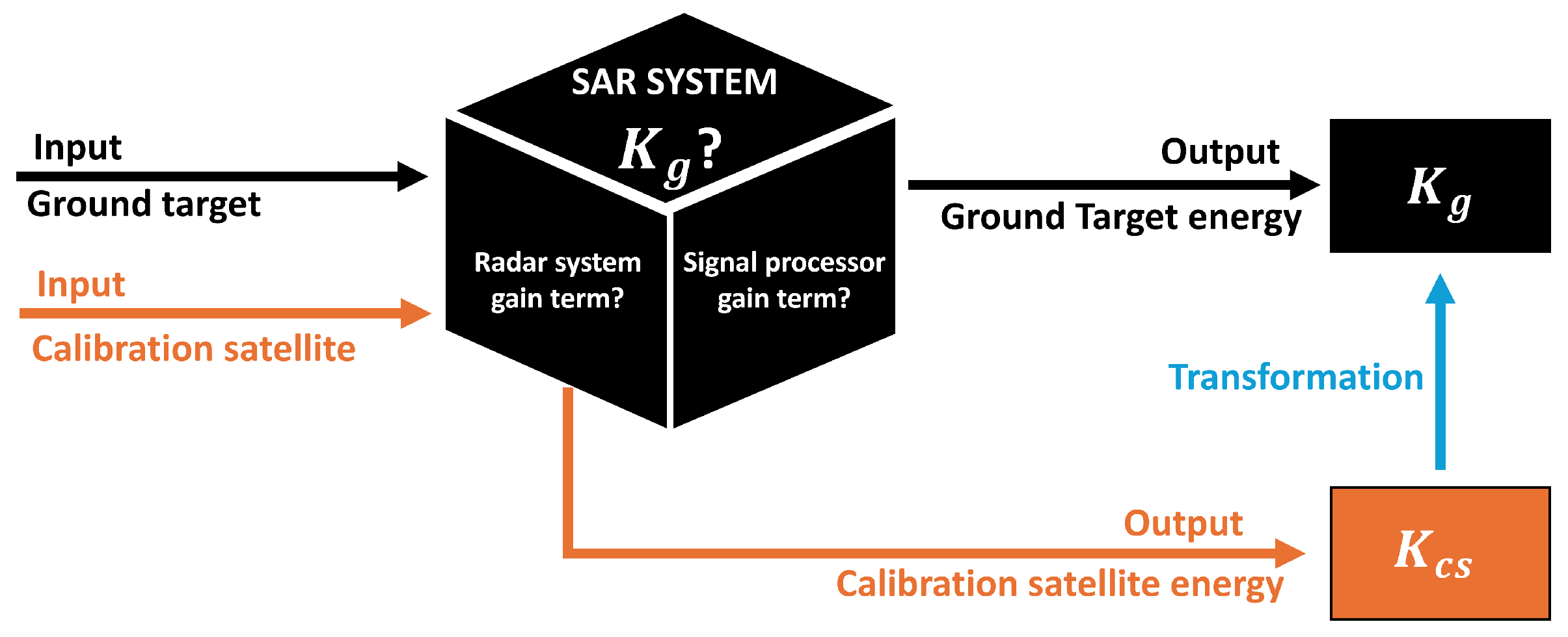
Traditional SAR radiometric calibration treats the system as a single “black box,” estimating overall gain by extracting point target energy from the focused image. This approach inherently combines the effects of both radar hardware and the signal processor, making it difficult to separate their individual contributions. In this context, we propose a novel space-based absolute radiometric calibration method using a small calibration satellite flying in a designed orbital formation with the SAR satellite. The calibration satellite that carries a passive reflector or an active transponder (with known RCS) can periodically fly across the SAR beam. The SAR satellite can observe and image the calibration satellite under the side-looking acquisition geometry, enabling derivation of calibration factors from the received signal, which can directly characterize the radar system gain terms. Meanwhile, considering the differences in the imaging processing chains and acquisition parameters between the calibration satellite and the ground scene, the calibration factor derived from the calibration satellite can be transformed and applied to calibrate the ground scene image. By separating the radar system gain from the signal processor gain in the absolute calibration process, this method deconstructs the traditional “black box,” allowing for a more accurate characterization of the SAR hardware’s intrinsic radiometric response. Moreover, the entire calibration process is performed in the space environment, free from distortions caused by atmosphere, ionosphere, ground clutter, multipath effects and ambiguities, ensuring a truly end-to-end calibration process. The proposed space-based calibration method is not only applicable to LEO SAR but can also be extended to MEO, GEO, and deep space exploration SAR. Besides SAR satellites, if the payload on the calibration satellite is more versatile, this method can also be applied to other microwave remote sensing sensors, such as Radar Altimeters and Scatterometers.

To simplify modeling, the derivations in this paper assume that the antenna center of the SAR satellite is positioned at the center of gravity. The acquisition geometry is assumed to be right-looking, although the methodology and formulas are applicable to left-looking configurations as well. Additionally, it is assumed that the radar satellite can adjust its attitude in yaw, pitch, and roll angles. To enhance readability, the SAR satellite or Sensor satellite to be calibrated will be abbreviated as SS and the calibration satellite is referred to as CS.

The remainder of this paper is organized as follows. Section 2 outlines the fundamental concepts and principles of the space-based absolute radiometric calibration approach. Section 3 details the calibration system configuration and the orbital selection strategy for the CS. Section 4 describes the imaging simulation process and subsequent analysis of the CS. Section 5 provides a detailed explanation of the calibration method, including the computation of calibration factors derived from the CS and the transformation of these factors for ground scene image calibration. Section 6 presents experimental results that validate the effectiveness of the calibration factor transformation. Section 7 discusses the potential challenges associated with the proposed space-based method and presents corresponding solutions. It also explores possible directions for future research within this framework. Finally, Section 8 concludes this work.

2. Basic Concept and Principles

2.1. Radiometric Calibration

The generation of an SAR image involves a series of processes, including signal generation by the radar hardware, propagation and scattering of the signal within the observed scene, echo reception by the radar system, and subsequent image processing by the signal processor. In general, the SAR system is considered as a linear system, and the relationship between the pixel value of the SAR power image and the target/scene radar cross-section can be derived from the radar equation, and expressed by the following formula:

$$P_r={\displaystyle \frac{P_t{\lambda }^2{G}_t^A\left({\theta }_{el},{\theta }_{az}\right)G_r^A\left({\theta }_{el},{\theta }_{az}\right)G_r^E{G}_p}{{\left(4\pi \right)}^3{R}^4{L}_s{L}_a}}\sigma$$

(1)

where $P_r$ is the pixel value of focused SAR power image; $P_t$ is the radar transmit power; $\lambda$ is the wavelength; $G_r^A\left({\theta }_{el},{\theta }_{az}\right)$ and $G_t^A\left({\theta }_{el},{\theta }_{az}\right)$ are the receive and transmit antenna gain, respectively; ${\theta }_{el}$ and ${\theta }_{az}$ are elevation angle and azimuthal angle at which each point on the ground is illuminated, respectively; $G_r^E$ is the overall electronic gain of radar receiver; $G_p$ is the overall signal processor gain; R is the radar–target distance; $L_s$ is the system loss term; $L_a$ is the two-way atmospheric loss; and $\sigma$ represents the RCS of the observed target/scene. The terms $\lambda$, R, and $L_s$ are all well known or easily measured and calibrated. Attenuation $L_a$ caused by atmospheric propagation typically affects higher-frequency SAR signals significantly and can be predicted by models of radar propagation. Significant measurement errors come only from the uncertainty of radar system gain ($P_t$, $G_t^A\left({\theta }_{el},{\theta }_{az}\right)$, $G_r^A\left({\theta }_{el},{\theta }_{az}\right)$, $G_r^E$) and signal processor gain ($G_p$).

To better characterize the total transfer function (the overall gain term of radar system and signal processor) of the SAR system, a constant K is explicitly defined as Equation (2), which is known as the absolute calibration factor. For a stable SAR system, K remains constant within a specific linear dynamic range.

$$K={\displaystyle \frac{P_t{\lambda }^2{G}_t^A\left({\theta }_{el},{\theta }_{az}\right)G_r^A\left({\theta }_{el},{\theta }_{az}\right)G_r^E{G}_p}{{\left(4\pi \right)}^3{R}^4{L}_s{L}_a}}$$

(2)

The purpose of SAR radiometric calibration is to establish a consistent relationship between a radar image and the scattering characteristics of observed scenes through the total transfer function of the SAR system. The SAR radiometric calibration process typically consists of two aspects: relative radiometric calibration and absolute radiometric calibration. Relative radiometric calibration is typically performed to ensure the system’s total transfer function remains constant without the need to measure the specific value of the calibration factor K, and without converting the SAR data to an absolute physical scale. The process typically involves multiple components, including internal loop calibration to monitor and stabilize key system parameters such as transmit power $P_t$ and receiver gain $G_r^E$, in-orbit antenna pattern measurement and compensation to correct for angular-dependent gain variations $G_t^A\left({\theta }_{el},{\theta }_{az}\right)$ and $G_r^A\left({\theta }_{el},{\theta }_{az}\right)$.

Absolute radiometric calibration is the final step in the calibration process, aiming to obtain an accurate value for the calibration factor K and convert the SAR image into absolute physical quantities. The value of the calibration factor K is typically determined through external calibration techniques. Artificial standard reference calibrators, such as passive corner reflectors or active transponders with known RCS, are deployed within the calibration sites, and the impulse response energy derived from standard reference calibrators in the final focused SAR image is used to calculate the calibration factor K. In this process, the radar system can essentially be regarded as a black-box system, as the errors of signal processor gain $G_p$ cannot be distinguished from the errors of relative calibration; this inherent coupling makes it difficult to attribute calibration errors to specific system components.

2.2. Principles of Space-Based Method

This subsection introduces the basic principles and theoretical foundation of the space-based absolute radiometric calibration method. According to the principle of absolute radiometric calibration, a prerequisite for deriving the calibration factor is the availability of a focused image that containing a well-focused reference target. Therefore, the space-based calibration method should also meet this fundamental requirement.

Assuming the CS carries a well-characterized and stable onboard calibration instrument (such as passive reflector or active transponder), its primary objective is to provide a detectable calibration reference for the SAR satellite (SS), thereby enabling quantitative assessment of the SS’s radiometric performance. To allow the SS to receive the echo data containing the calibration signal from the CS, the CS’s orbit should be carefully considered. The CS must traverse the SAR beam with sufficient dwell time to meet coherent integration requirements, while maintaining a periodic revisit to establish a stable and repeatable calibration geometry.

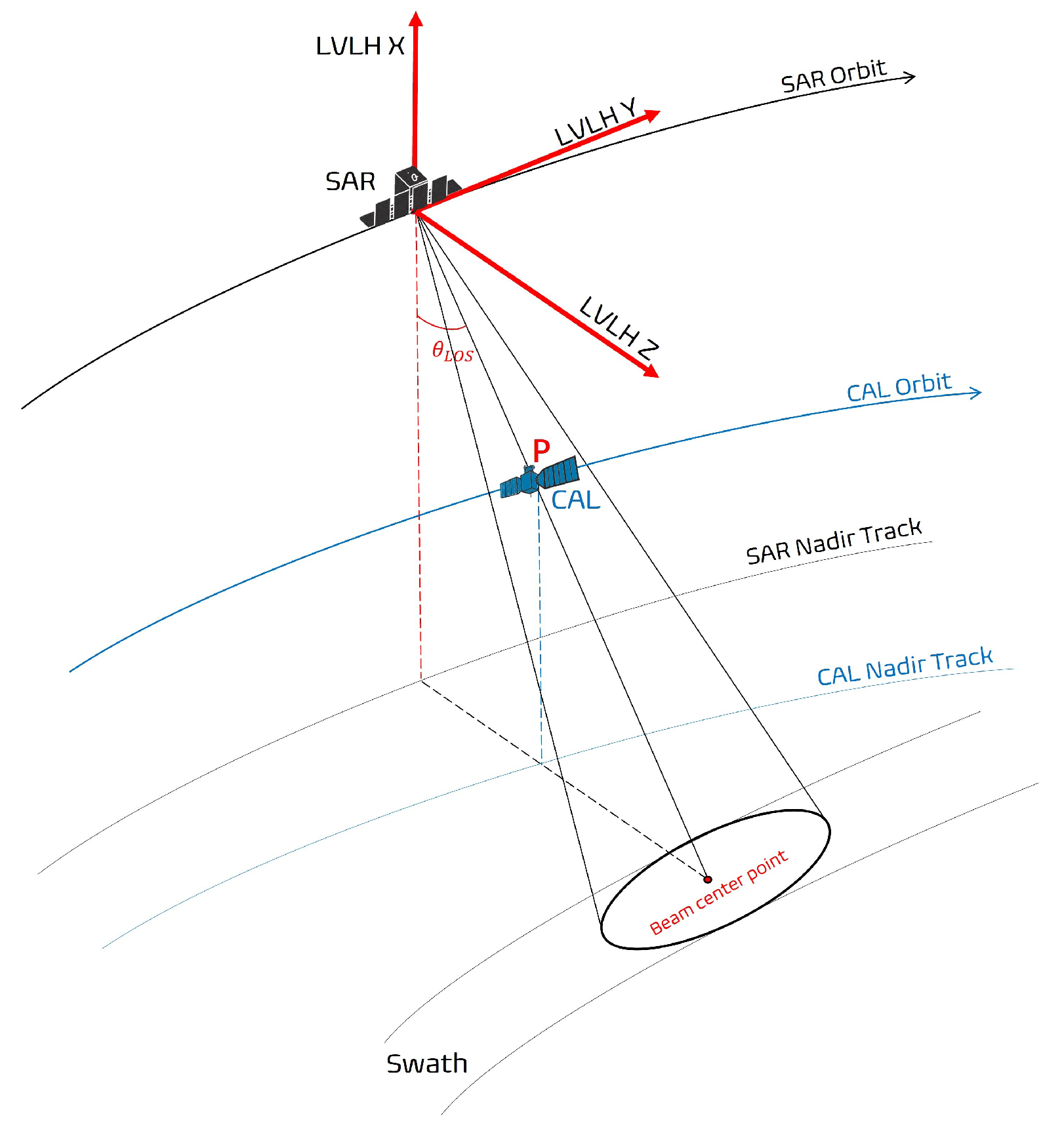
Figure 1 illustrates the basic orbital geometry for the space-based calibration. The SS operates in the side-looking mode, the CS follows a designated orbit, moving along the same prograde orbit as the SS, and periodically crosses through the SS beam in the azimuth direction. During these crossing events, the CS’s echo falls within the SAR receiving echo gate, and the satellite’s motion within the SAR beam meets the coherent accumulation time requirements for SAR imaging. In other words, the SS can observe and image the CS under the side-looking acquisition geometry.

As a result, the received echo is a superposition of the CS echo and the ground scene echo. Through appropriate data processing, the energy corresponding to the CS can be extracted, and the associated calibration factor $K_{\mathit{cs}}$ under the specific processing chain can be derived. This factor characterizes the overall system gain and can be expressed as follows:

$$K_{cs}={\displaystyle \frac{P_t{\lambda }^2{G}_t^A\left({\theta }_{el},{\theta }_{az}\right)G_r^A\left({\theta }_{el},{\theta }_{az}\right)G_r^E{G}_p^{cs}}{{\left(4\pi \right)}^3{R}_{cs}^4{L}_s}}$$

(3)

where $R_{cs}$ is the distance between the CS and SS, and $G_p^{cs}$ represents the processing gain of the CS signal.

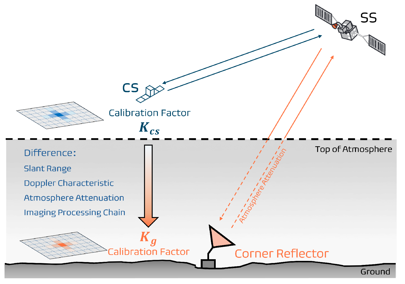
Conducted entirely in space, the calibration process is free from distortions caused by atmosphere, ionosphere, ground clutter, multipath effects and ambiguities, ensuring the calibration factor $K_{\mathit{cs}}$ can directly and accurately reflect the characteristics and uncertainties of the radar system gain terms. However, due to differences in the imaging processing chain and acquisition parameters between the CS and typical ground targets, $K_{\mathit{cs}}$ cannot be directly applied to the radiometric calibration of ground scene data. To obtain an absolute calibration factor $K_g$ that is valid for ground targets, $K_{\mathit{cs}}$ must be adjusted accordingly. This adjustment accounts for the differences in parameters and imaging processing chains between the spaceborne CS imaging configuration and the ground observation scenario, as illustrated in Figure 2. Since the processing gain can be quantitatively analyzed, the calibration factor $K_{\mathit{cs}}$ can be correspondingly related to or transformed into $K_g$, as illustrated in Figure 2 and expressed as follows.

$$K_g=K_{cs}·{\displaystyle \frac{1}{L_a}}·{\displaystyle \frac{G_p}{G_p^{cs}}}·{\left({\displaystyle \frac{R_{cs}}{R}}\right)}^4$$

(4)

Therefore, the overall calibration strategy can be conceptually divided into two stages: (a) The in-orbit calibration using $K_{\mathit{cs}}$ enables accurate characterization of radar system gain and uncertainty in a space environment; and (b) through appropriate transformation and correction, $K_{\mathit{cs}}$ can be converted into a ground-valid calibration factor $K_g$, which supports the radiometric calibration of actual ground imagery products.

The above content provides a conceptual and theoretical framework for the space-based radiometric calibration method. To implement this approach and achieve optimal performance, two key technical issues must be addressed:

• Orbit selection strategy of the calibration satellite. Since the orbital elements of SAR satellites are typically optimized for Earth observation missions, and the parameters of SAR beams are usually fixed and well-defined, it is essential to select an appropriate CS orbit strategy, which should ensure geometric feasibility and enable frequent and reliable calibration of one or multiple SAR satellites.
• Calibration factor processing and transformation methods. Significant differences exist between the CS and ground-based imaging scenarios in terms of imaging environment, signal propagation path, acquisition parameters, and processing chains under the same SAR beam. Therefore, the calibration factor obtained from the CS cannot be directly applied to SAR radiometric calibration. It is necessary to develop transformation models of calibration factors that account for these differences, incorporating specific imaging algorithms and system parameters.

3. Calibration Configuration and Orbit Selection Strategy

To implement the proposed space-based radiometric calibration method, it is essential to design a feasible and effective calibration system. This section provides a high-level description of a feasible calibration system focusing on two key aspects: Calibration Configuration and orbit selection strategy. The calibration configuration includes the type and RCS requirement of CS payload, as well as the SS-to-CS distance that determines whether the CS echo can fall accurately within the SAR receiver’s window under the existing SAR beam arrangement. Regarding orbit design, it is necessary to ensure that the CS can periodically enter the SAR antenna’s beam footprint and maintain a stable geometric relationship and sufficient dwell time, enabling the SS to receive effective echoes and thereby ensuring the accuracy and frequency requirements of the radiometric calibration.

3.1. Calibration Configuration

In traditional ground-based calibration methods, trihedral corner reflectors are commonly used due to their high reflectivity. However, they require precise alignment with the radar beam before each calibration. Considering that the CS can only achieve beam alignment through attitude adjustment after entering orbit, an isotropic calibration sphere can be used as the calibration payload to reduce system complexity and minimize imaging and calibration errors caused by beam misalignment. Although the calibration sphere has a smaller RCS than a trihedral corner reflector of the same size, the significantly shorter distance between SS and CS, compared to the distance between the SS and ground target, enables the sphere to achieve the required RCS with a more compact design, thereby ensuring a satisfactory signal-to-clutter ratio (SCR) for calibration requirement.

To improve calibration accuracy, a SCR greater than 35 dB is typically required in the calibration area, which places higher demands on the RCS of the calibration equipment. During the calibration campaign of TerraSAR-X, triangular-faced trihedral corner reflectors in two sizes are used, which feature different radar cross sections (symbol ${\sigma }_c$) at the center frequency of 9.65 GHz [23]:

• Inner leg length of 1.5 m, ${\sigma }_c=$ 43.4 dBm²
• Inner leg length of 3.0 m, ${\sigma }_c=$ 55.5 dBm²

According to the (monostatic) radar equation, the target echo power $P_r$ at the radar antenna output is calculated as follows.

$$P_r={\displaystyle \frac{P_t·{\lambda }^2·G_{Tx}·G_{Rx}·G_r^E·{\sigma }_c}{{\left(4\pi \right)}^3·R^4·L_s·L_a}}$$

(5)

where the received power $P_r$ is expressed in terms of the transmit power $P_t$, the maximum receive and transmit antenna gain $G_{Rx}$ and $G_{Tx}$, the radar receiver gain $G_r^E$, the wavelength $\lambda$, the radar-target distance R, the system loss term $L_s$, the two-way atmospheric loss $L_a$ and the point target RCS ${\sigma }_c$. The power calculation is discussed with respect to a TerraSAR-X like illumination of corner reflectors with the parameters in

Table 1. TerraSAR-X-like System Parameters for Corner Reflector Illumination.

Parameter	Value
Wavelength $\lambda$	0.03106 m
Transmit power $P_t$	2200 W
Tx antenna gain $G_{Tx}$	36.3 dB
Rx antenna gain $G_{Rx}$	36.3 dB
Radar receiver gain $G_r^E$	20 dB
SS-to-reflector distance R	600 km
System loss $L_s$	1 dB
Two-way atmospheric loss $L_a$	2 dB

. It is important to note that when using this equation to calculate the echo power of the CS, atmospheric loss is not considered.

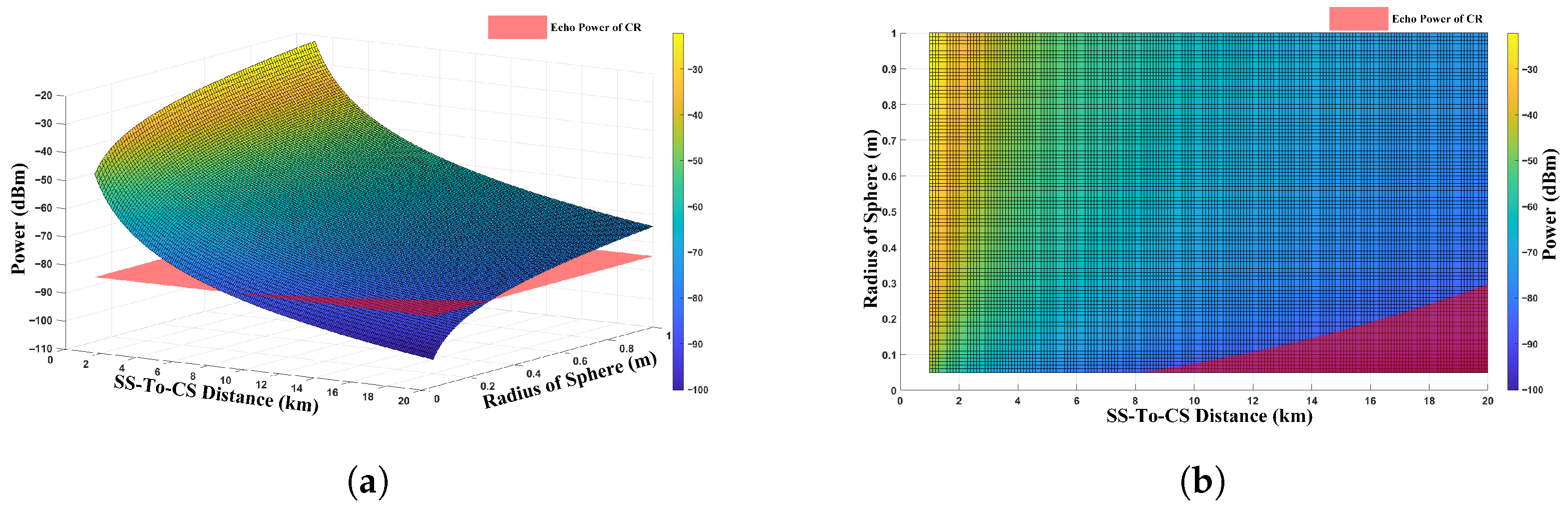
Assuming the distance range from the satellite to the calibration sphere (SS-To-CS) is (1 km, 20 km), and the radius of the sphere is (0.05 m, 1 m). Figure 3 provides $P_r$ for the two-way measurement with the calibration sphere on-board the CS as a function of R (SS-To-CS distance) and a (radius of calibration sphere) and the resulting $P_r$ of −84.73 dBm for the on-ground 3 m corner reflector is shown by the red plane in Figure 3. Analysis of Figure 3 demonstrates that optimal selection of calibration sphere radius and SS-to-CS distance results in significantly stronger echo power from the CS compared to ground targets under identical observation conditions. This enhanced backscatter enables the CS to provide superior SCR performance compared with ground-based corner reflectors, consequently satisfying more demanding measurement accuracy specifications. Therefore, small-sized calibration spheres are suitable for space-based calibration method and can be easily implemented in practice.

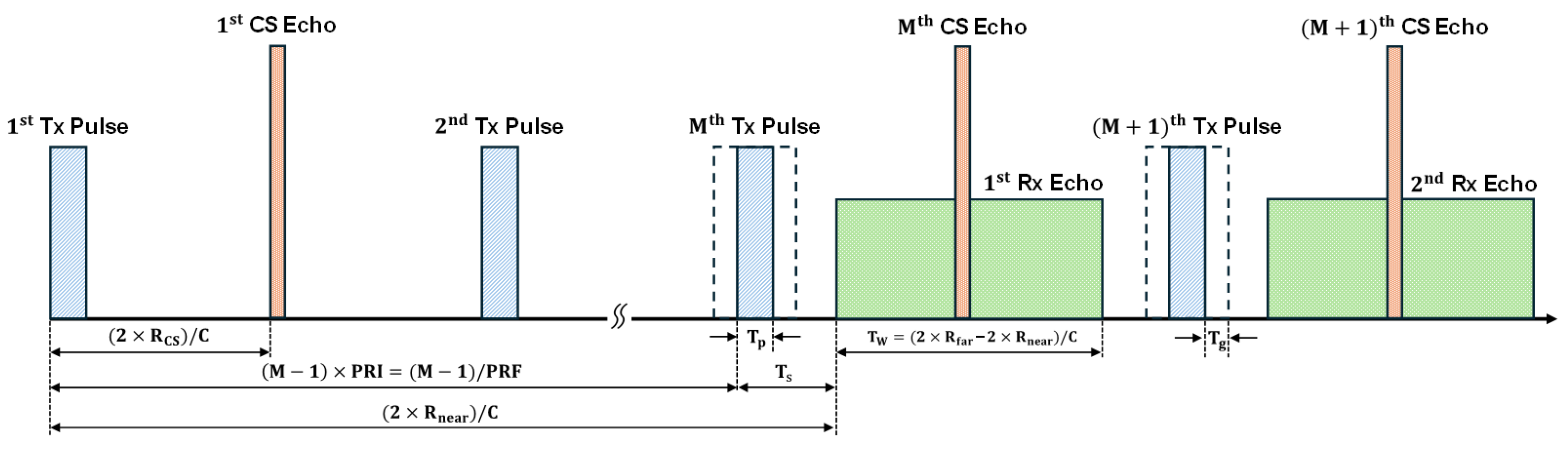
Existing SAR beam arrangements are specifically optimized for terrestrial observation scenarios, where nadir interference and pulse blocking are usually avoided through constrained pulse repetition frequency (PRF) selection in the SAR system design. The current system design, however, does not incorporate provisions for receiving CS echoes. To perform in-orbit radiometric calibration using CS, it is essential to ensure that the CS echo can be received by the SAR system; i.e., the echo must strictly fall within the receiving time window. Since the echo arrival time is determined by the SS-To-CS distance, the SS-To-CS distance must not only satisfy the aforementioned receiving power requirements but also comply with the existing SAR transmit-receive window design.

Figure 4 illustrates a typical SAR satellite timing diagram, where $T_p$ is the pulse width and $T_g$ is the guardband width. Following the transmission of the first pulse, the satellite typically delays the echo reception window activation by several pulse repetition intervals (PRIs) to capture the ground return of that initial pulse. As shown in the figure, within PRI, the receiver is turned on after $T_s$ seconds from the start of transmission, to receive the echo of the corresponding transmitted pulse. Then, it is turned off after $T_w$ seconds of sampling, which results in a unambiguous swath width of $D_{\mathrm{swath}}=R_{far}-R_{near}$, which is approximately equal to $c{T}_{\mathrm{w}}/2$, provided that the elevation pattern covers the swath width.

The PRF of most spaceborne SAR satellites typically ranges from 3500 to 7000 Hz, corresponding to a PRI of 142.86 to 285.71 μs. For a CS with SS-to-CS distance range of 1–20 km, the corresponding echo time delay is 6.67 to 133.33 μs, which implies that each pulse echo of the CS will arrive within its corresponding PRI. Therefore, to ensure the CS echoes fall within the reception window, the SS-to-CS distance $R_{cs}$ must satisfy

$$\left\{\begin{array}{cc}\hfill {\displaystyle \frac{2R_{cs}}{c}}+(M-1)PRI& >{\displaystyle \frac{2R_{near}}{c}}\hfill \\ \hfill {\displaystyle \frac{2R_{cs}}{c}}+(M-1)PRI& <{\displaystyle \frac{2R_{far}}{c}}\hfill \end{array}\right.$$

(6)

where $M=floor\left({\displaystyle \frac{2R_{near}}{c·PRI}}\right)$ is an integer number, which represents the number of intervening pulses. Consequently, as shown in Figure 4, when the SS opens its first reception window during the $M^{\mathrm{th}}$ PRI, the $1^{\mathrm{st}}$ Rx echo contains both the $M^{\mathrm{th}}$ CS echo from and the first ground echo. This means the echo from CS is superimposed to the echo from a scatterer in the ground scene at $R_0$, where $R_0$ is calculated as follows:

$$R_0=(M-1)\times PRI\times c/2+R_{cs}$$

(7)

3.2. Orbit Selection Strategy of the Calibration Satellite

Traditional ground-based radiometric calibration relies on fixed ground calibration sites and reference targets. Since the locations of these ground calibration sites are stationary and precisely known, SAR satellites in orbit only need to consider the satellite-to-ground geometric relationship, which is typically addressed during the overall planning phase of the SAR satellite mission. In contrast, space-based radiometric calibration employs a dedicated CS as reference target and leverages the relative motion between these satellites and the SS to achieve calibration.

This approach reduces the reliance on ground-based calibration sites and targets, thereby improving the flexibility and spatial coverage of calibration. However, it also increases the technical complexity of the system. Nevertheless, to ensure the effective implementation of the proposed space-based method, the orbit design of CS must satisfy the following three fundamental conditions: (1) The CS must be illuminated by SAR antenna beam; (2) the slant range between SS and the CS must satisfy the radar timing that allows reliable signal reception; and (3) the relative motion should provide sufficiently frequent calibration opportunities.

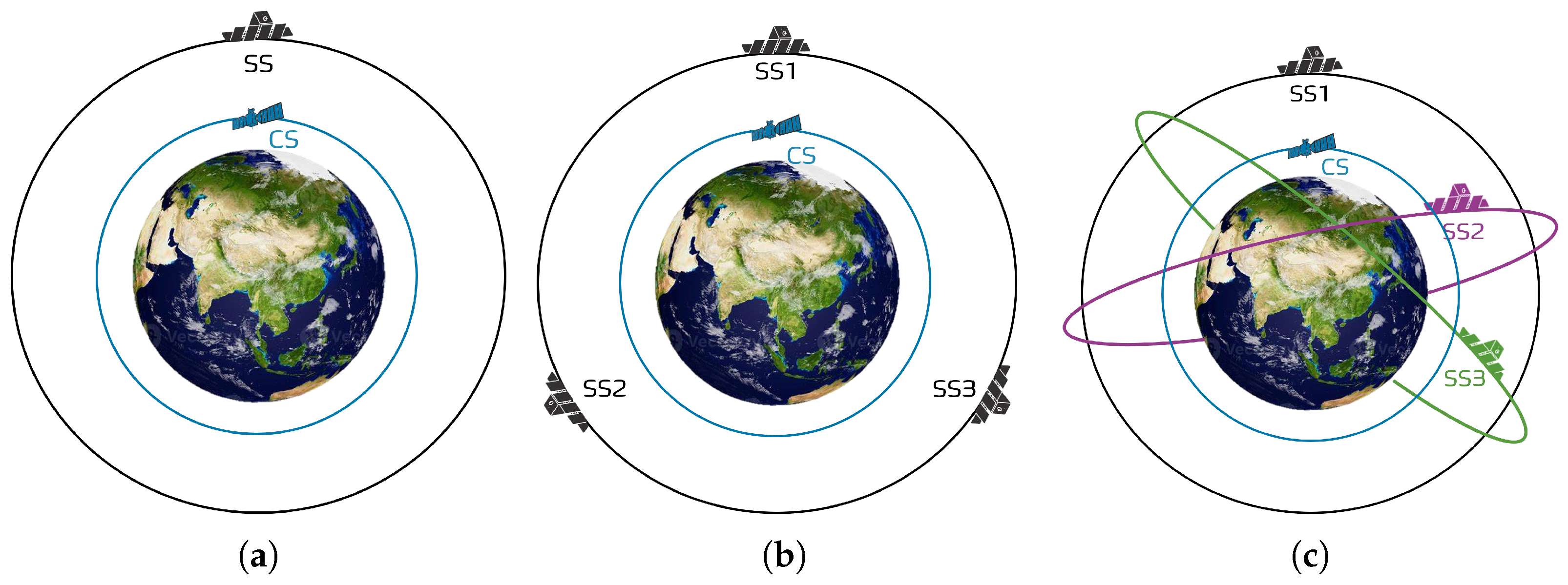
Consequently, it is essential to select an appropriate CS orbit strategy tailored to different calibration requirements, thereby enabling high-frequency space-based radiometric calibration. These calibration requirements, in turn, vary significantly depending on the number of SAR satellites involved and their orbital configurations. Therefore, the space-based radiometric calibration scenarios can be categorized into three levels of complexity as illustrated in Figure 5: The first scenario is calibration for a single SAR, which is the most fundamental and least complex type. The second scenario is calibration for multiple SARs within the same orbital plane, which extends and optimizes the single-satellite calibration approach. The third scenario is calibration for multiple SARs across different orbital planes, which is the most complex type, requiring comprehensive consideration of the spatial geometric relationships between different orbital planes.

(a)

Single SAR Calibration

In the single SAR radiometric calibration scenario, the CS should be designed to follow a formation-flying orbit with the same semi-major axis as the SS, ensuring identical orbital periods. By carefully adjusting other orbital elements, the CS can periodically traverse the SS’s beam coverage area along a predetermined trajectory, enabling precise radiometric calibration once per orbital cycle. This relative orbital configuration design is well-established, with common orbit types including the natural elliptical orbit and helix orbit [24,25,26,27].

(b)

Multi SARs calibration within the same orbit plane

In this calibration scenario, the CS operates in a lower orbit than the SS, resulting in a higher orbital velocity due to its smaller semi-major axis. With proper orbital design, the CS can periodically pass through the beams of multiple SSs within the same orbital plane, enabling a single CS to calibrate all SSs in that plane. Both the CS and SS follow periodic motion. Set $T_1$ and $T_2$ denote the orbital periods of the SS and CS, respectively. Over a time interval corresponding to the least common multiple (LCM) of $T_1$ and $T_2$, the CS returns to its initial relative position, initiating a new calibration cycle. This orbital design method is well-established, with common types of orbits, such as the spiral cruising orbit and traveling ellipse orbit [28].

(c)

Multi SARs calibration across different orbit planes

This calibration scenario is highly complex, with the main challenge being that the CS must perform high-precision orbital maneuvers to simultaneously calibrate multiple SSs in different orbital planes. A solution could involve optimizing the satellite’s orbit design using methods similar to those for non-coplanar multi-target space rendezvous, allowing it to dynamically adjust its orbit and calibrate SS across multiple planes. To achieve this, the CS must have advanced maneuverability, enabling it to move flexibly in multiple directions [29,30].

3.3. Orbit Simulation for Different Calibration Scenarios

A fundamental assumption adopted throughout this study is that the chief satellite (i.e., the SAR satellite) does not perform any dedicated orbit maneuvers for radiometric calibration purposes. This assumption reflects a common operational constraint in real SAR missions, where satellite maneuvers are primarily driven by imaging requirements and payload scheduling. Considering the associated operational complexity and fuel costs, it is generally impractical to introduce additional maneuvers solely for radiometric calibration.

Under this assumption, the required calibration geometry is determined entirely by the orbit design of the calibration satellite (CS). When the orbital elements of the SAR satellite are known, an appropriate selection of the CS orbital elements can lead to a relative configuration that remains bounded over an extended period of time. This property has been well established in the formation-flying literature; for example, Schaub and Alfriend [31] introduced the concept of J₂-invariant relative orbits. Within the time interval over which the relative configuration remains bounded (e.g., tens to hundreds of orbital periods), the CS can exploit its natural relative motion to periodically traverse the SAR beam coverage, thereby providing repeated calibration opportunities without requiring maneuvering of the SS and CS.

It should be noted, however, that such bounded relative configurations are not maintained indefinitely in practical missions. Due to long-term orbital perturbations, periodic formation maintenance is ultimately required. The investigation of orbit maintenance and control strategies constitutes a problem of a different nature from the feasibility assessment of the calibration method considered in this paper. Therefore, optimal orbit design under perturbations and long-term formation maintenance strategies are beyond the scope of the present study and will be addressed in future work.

From this perspective, the calibration process can be regarded as a cooperative observation problem based on orbit prediction and mission planning. By analyzing the predicted relative trajectory of the CS with respect to the SAR beam coverage, suitable orbital arcs and calibration time windows can be identified. During these windows, the SAR satellite activates the corresponding beam configuration to perform calibration measurements. Conceptually, this process is analogous to the mission planning of ground-based radars observing space targets.

Satellite formation flying designs are commonly derived from the linearized equations of relative motion under the two-body dynamical assumption, also known as Hill’s equations. Within this framework, existing relative orbit design methodologies can be broadly categorized into algebraic methods, which formulate relative motion equations in a local coordinate system based on the absolute equations of motion, and geometric methods, which describe relative motion using the orbital elements of the chief and deputy spacecraft. Detailed formulations of these approaches can be found in [32,33,34] and are not repeated here.

It should be emphasized that this study does not aim to develop or compare specific relative orbit design or formation control strategies. Instead, the focus is placed on the investigation of space-based SAR radiometric calibration methodologies. Accordingly, the orbit-related analysis is intentionally limited to a principle-level study that supports the feasibility and measurement consistency of the proposed calibration concept.

Consistent with this scope, orbital simulations are performed under a simplified two-body assumption considering the first two calibration scenarios introduced earlier. The initial relative configurations adopted in these simulations are intended to demonstrate the feasibility of the proposed calibration methodology and to provide a consistent orbital basis for subsequent echo simulations. Numerical simulations are therefore conducted for Scenarios 1 and 2, with the corresponding parameters summarized in

Table 2. SAR and cal satellite orbit elements.

Satellite	a (km)	e	Ω (deg)	i (deg)	ω (deg)	M (deg)
SS1	7000	0	0	97	90	0
SS2	7000	0	0	97	90	120
SS3	7000	0	0	97	90	240
CS1	7000	0.00096	0	97.0338	90	0
CS2	6990	0.001	0	97.086	90	0

, where a denotes the semi-major axis, e the eccentricity, $\Omega$ the right ascension of the ascending node, i the inclination, $\omega$ the argument of perigee, and M the true anomaly.

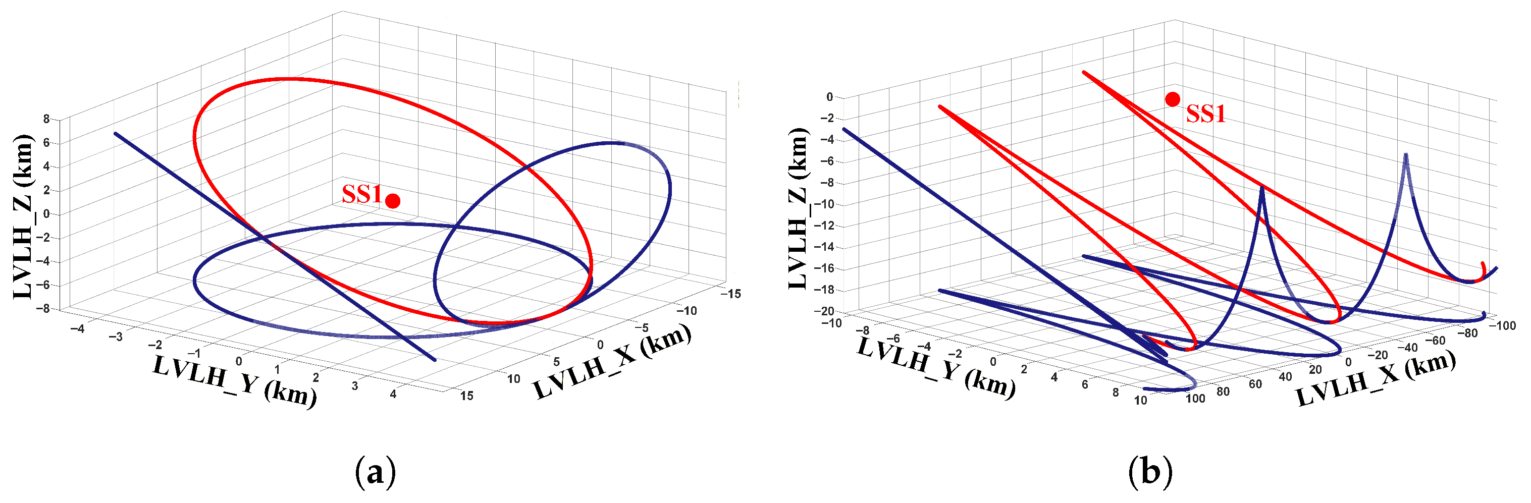
SS1, SS2, and SS3 are three SAR satellites co-located within the same orbital plane. CS1 is the calibration satellite for calibration scenario 1, with an orbital period synchronized to SS1 to provide dedicated calibration services exclusively for SS1. CS2 serves as the calibration satellite for calibration scenario 2, enabling multi-satellite calibration across the entire orbital plane, delivering synchronized reference measurements for all three SAR satellites (SS1, SS2 and SS3).

Based on the simulation orbit elements presented in Table 2, Figure 6 illustrates the relative configurations between CS1, CS2, and SS1, along with their projections on each plane of the SS1 LVLH coordinate system. It can be seen that CS1 maintains a periodic elliptical orbit around SS1, while CS2 follows a quasi-periodic parabolic trajectory away from SS1, which essentially represents a degenerate form of a three-dimensional helical trajectory.

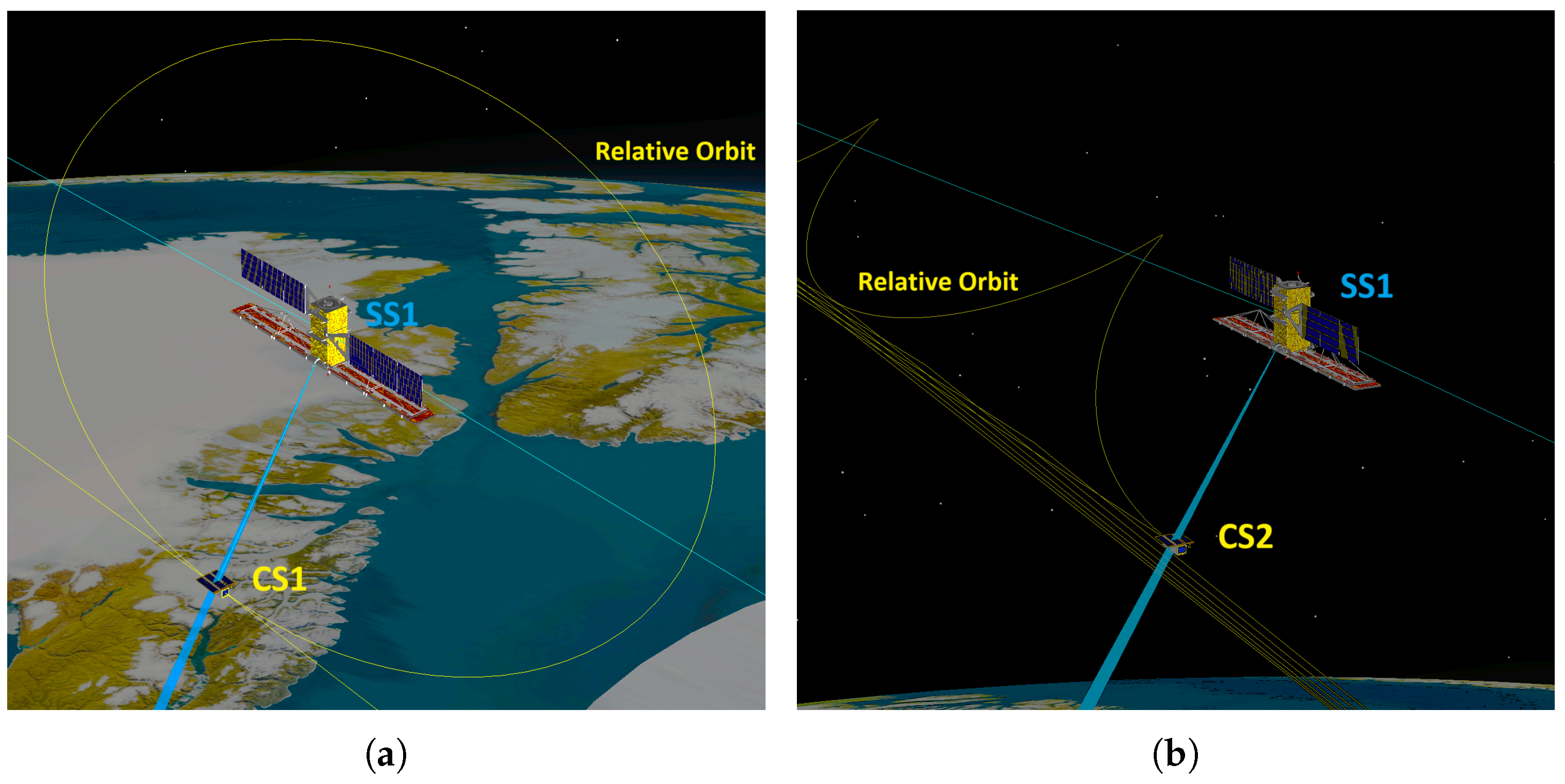
For further validation, a scenario containing the SAR and CAL satellite is created through STK (Satellite Tool Kit), as shown in Figure 7. In this scenario, a beam with a 3 dB beamwidth of $Az\ast Ra=$ 0.2° ∗ 2° and side-looking offset angle of 32° was inserted to SS1, SS2 and SS3 to analyze the appropriate calibration opportunities.

Table 3. Access events between CS1 and the SAR sensor (SS1) during the simulation period from 17 Mar 2025 to 18 Mar 2025. The table lists all access intervals when the calibration satellite is within the antenna beam. Start and stop times are given in UTCG, and the duration represents the length of each access event in seconds.

Access	Start Time (UTCG)	Stop Time (UTCG)	Duration (s)
1	2025-03-17 04:00:00.000	2025-03-17 04:00:00.947	0.947
2	2025-03-17 05:37:07.573	2025-03-17 05:37:09.463	1.890
3	2025-03-17 07:14:16.090	2025-03-17 07:14:17.979	1.890
4	2025-03-17 08:51:24.606	2025-03-17 08:51:26.500	1.894
5	2025-03-17 10:28:33.123	2025-03-17 10:28:35.013	1.890
6	2025-03-17 12:05:41.640	2025-03-17 12:05:43.530	1.890
7	2025-03-17 13:42:50.156	2025-03-17 13:42:52.048	1.892
8	2025-03-17 15:19:58.673	2025-03-17 15:20:00.563	1.890
9	2025-03-17 16:57:07.189	2025-03-17 16:57:09.080	1.892
10	2025-03-17 18:34:15.707	2025-03-17 18:34:17.597	1.890
11	2025-03-17 20:11:24.224	2025-03-17 20:11:26.114	1.890
12	2025-03-17 21:48:32.741	2025-03-17 21:48:34.630	1.890
13	2025-03-17 23:25:41.257	2025-03-17 23:25:43.147	1.890
14	2025-03-18 01:02:49.774	2025-03-18 01:02:51.664	1.890
15	2025-03-18 02:39:58.291	2025-03-18 02:40:00.181	1.890

summarizes the access count between CS1 and SS1 sensor fence within a 24 h time window, while

Table 4. Access events between CS2 and multiple SAR sensors (SS1–SS3) during the simulation period. Each entry corresponds to a beam-crossing event. Start and stop times are given in UTCG, and the duration represents the length of each access event in seconds.

Sensor	Access	Start Time (UTCG)	Stop Time (UTCG)	Duration (s)
SS1	1	2025-03-17 04:00:00.000	2025-03-17 04:00:01.127	1.127
SS1	2	2025-09-21 17:11:44.826	2025-09-21 17:11:47.045	2.219
SS2	1	2025-07-31 08:14:24.462	2025-07-31 08:14:26.683	2.221
SS2	2	2026-02-04 21:26:10.397	2026-02-04 21:26:12.618	2.221
SS3	1	2025-05-08 12:57:19.283	2025-05-08 12:57:21.504	2.221
SS3	2	2025-11-13 02:09:05.218	2025-11-13 02:09:07.439	2.221

records the access count of CS2 with respect to SS1, SS2, and SS3 beam over a one-year duration.

Simulation results indicate that CS1, which has the same orbital period as SS1, can calibrate SS1 once per orbital cycle, enabling high-frequency calibration. CS2, on the other hand, calibrates SSs within the same orbital plane twice per year, which is relatively less frequent than CS1. Consequently, CS2 requires a much longer time to traverse the entire orbit. To enhance calibration frequency, additional calibration satellites can be deployed, or the semi-major axis difference can be increased to accelerate orbital coverage.

The simulation results demonstrate that, through appropriate orbit or formation design, the CS can operate in a specific relative configuration with SS, such as the basic side-looking geometry, while maintaining a relatively high calibration frequency. Although the simulations are based on simplified conditions, they are sufficient to support the imaging simulation and analysis of the CS and to validate the subsequent measurement and conversion of calibration factor.

4. Imaging Simulation and Analysis of CS

Based on the orbital simulation results of Calibration Scenario 1 presented in the previous section, this section analyzes the observation geometry of the CS1 within the radar beam of the SS, and derives its slant range evolution and Doppler characteristics. An imaging simulation is then carried out to verify the imaging capability of the CS and the feasibility of energy extraction, which serves as a foundation for the subsequent calibration factor calculation and transformation.

To improve the realism of the simulation scenario, a composite scene consisting of a distributed background and the CS is constructed. The background simulates the statistical backscattering characteristics of natural terrain, based on actual SAR image data. The echo of the CS is generated according to its slant range evolution, with its signal placed in the raw data by mapping to the corresponding range gate at each sampling time. By linearly superimposing the CS echo onto the background echo, a SAR raw dataset is obtained, containing both background clutter and the CS signal for subsequent image processing and energy analysis.

4.1. Doppler Parameters Analysis

To accurately simulate and analyze the imaging performance of the CS, it is essential to examine its Doppler characteristics during the observation period. In calibration scenario 1, to ensure a basic side-looking observation geometry (i.e., the CS crosses the SAR antenna beam along the azimuth direction), the CS adopts an elliptical formation configuration with the same orbital period as the SS. Within the relative orbital period, the valid calibration arc corresponds to the time duration when the CS traverses the SAR beam (i.e., the “access period” in Table 3).

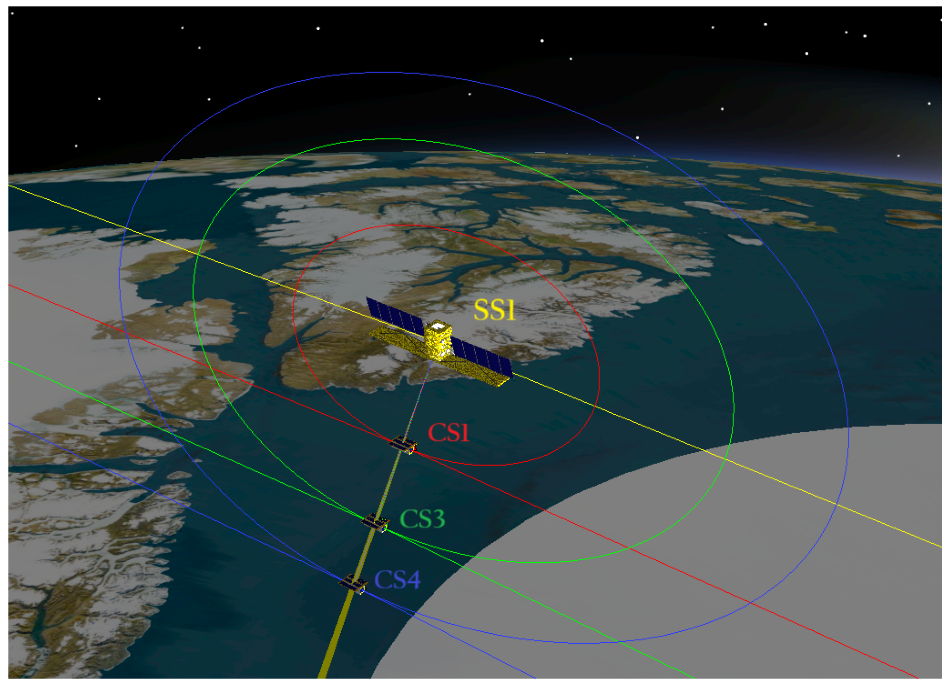
If the size of the elliptical formation configuration of the CSs varies, differences will arise in slant range variation, fly-around velocity, and the length of the calibration arc. These differences, in turn, lead to variations in the Doppler parameters. Therefore, to ensure the generality of the analysis, we select three CSs with different sizes of the elliptical formation configuration to examine their slant range evolution and Doppler frequency shift during the observation period, as shown in Figure 8, and their orbital elements are given in

Table 5. Orbit elements of CSs with different sizes of the elliptical formation configuration.

Satellite	a (km)	e	Ω (deg)	i (deg)	ω (deg)	M (deg)
SS1	7000	0	0	97	90	0
CS1	7000	0.00096	0	97.0338	90	0
CS3	7000	0.00168	0	97.06	90	0
CS4	7000	0.00225	0	97.081	90	0

(including CS1 analyzed in the previous section). This analysis provides insight into how the relative geometry affects Doppler characteristics under varying formation configurations.

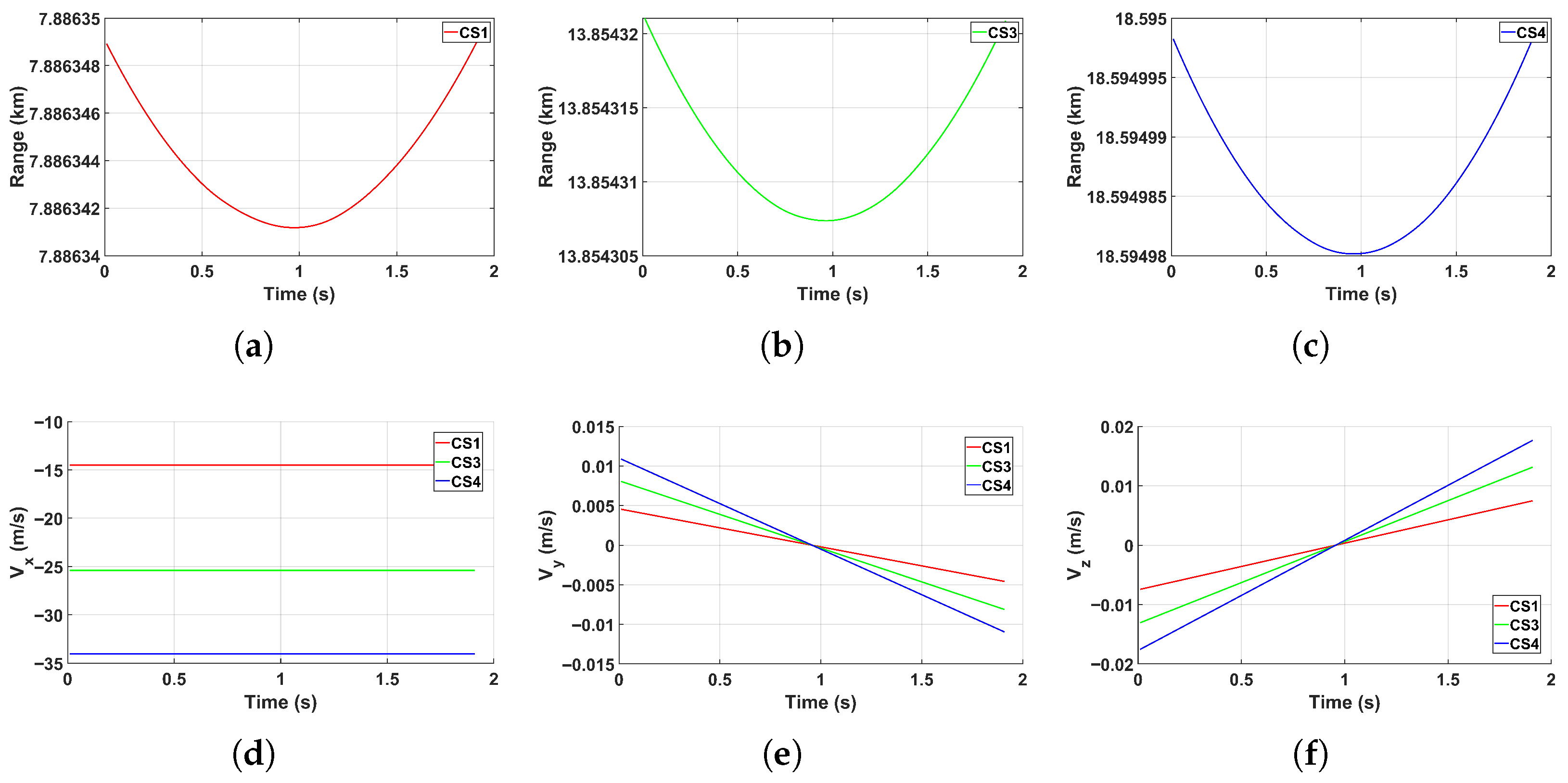
To further analyze the Doppler characteristics of the CSs, the range evolution and relative velocity of CS1, CS3, and CS4 are analyzed within their respective access periods. Figure 9a–c present the slant range evolution of the three CSs, while Figure 9d–f illustrate their velocity components along the X, Y, and Z directions in the SS1’s LVLH coordinate system. It can be observed that the range variation of all three CSs during their respective access periods is minimal, with a maximum variation less than 0.02 m, which is much smaller than the conventional SAR slant range resolution. Therefore, the range migration can be considered negligible and need not be corrected. Meanwhile, their relative velocities are primarily distributed along the X-axis of the SS-LVLH coordinate system, corresponding to the along-track (azimuth) direction. As the size of the elliptical formation increases, the relative velocity between the CS and the SAR satellite also increases. Nevertheless, the relative velocity remains significantly lower than the effective radar velocity for ground imaging. Therefore, even though the CS calibration arc length is much smaller compared to the synthetic aperture of ground target, its dwell time within the SAR beam remains sufficient, ensuring several seconds of echo signal acquisition.

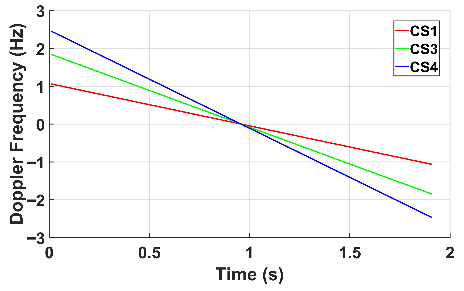
Based on the relative motion parameters, the Doppler frequency history of the three CSs during their respective access periods are analyzed, as shown in Figure 10. Under the same observation duration, the Doppler bandwidth of the CSs increases with the size of the elliptical formation configuration. Specifically, the Doppler bandwidths are 2.1236 Hz for CS1, 3.6905 Hz for CS3, and 4.9243 Hz for CS4. Although the Doppler bandwidth increases, it remains in the low-Hertz range—significantly narrower than the several-kilohertz bandwidths typically observed for ground targets in spaceborne SAR systems. This leads to a degradation in the azimuth resolution of the calibration satellite (CS), causing defocusing and energy spreading of point targets. Although precise azimuth focusing is not critical for energy extraction via integration methods, the reduced azimuth resolution necessitates an expanded integration window to ensure accurate energy estimation. However, this broader window inevitably introduces additional clutter and noise, ultimately affecting the precision of target energy retrieval. Therefore, directly applying conventional SAR imaging algorithms for ground targets to the CS echo is not appropriate. Even if a focused two-dimensional image is obtained, it may not be suitable for accurately extracting the energy of CS.

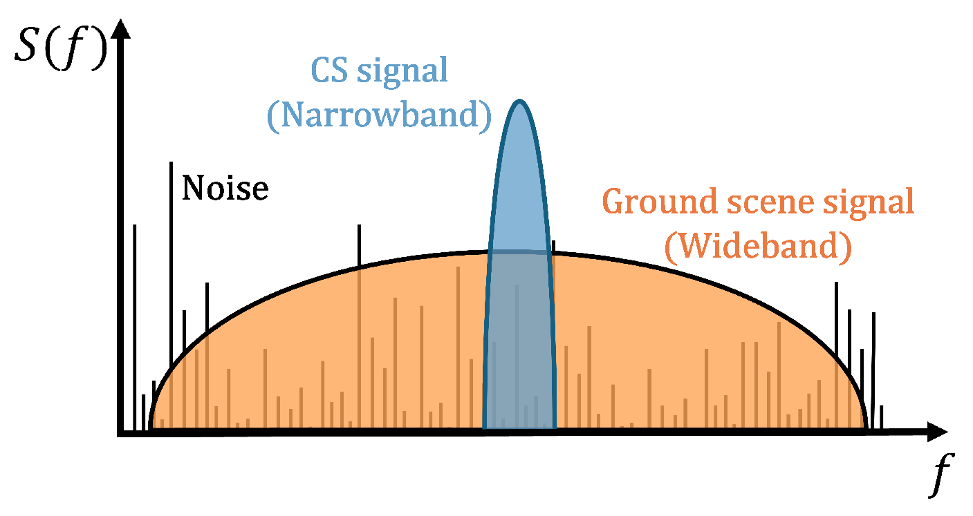
As previously analyzed, the CS echo essentially behaves as a point target signal with a narrow bandwidth embedded within the ground echo as shown in Figure 11, with a significantly higher energy level (see Section 3). This indicates that the CS energy is highly concentrated in the frequency domain—despite its narrow bandwidth, its spectral amplitude at corresponding frequency bins is very large. Moreover, the range migration of the CS during the imaging interval is negligible, meaning its energy remains confined within a single range gate after range compression. Moreover, due to the narrowband characteristic of the CS in the azimuth direction, applying a direct azimuth FFT to the range-compressed data can be interpreted as an equivalent coherent integration process (i.e., Pulse Doppler Processing). This operation transforms the signal into the Range-Doppler domain, where energy is coherently accumulated within specific frequency bins, thereby enabling effective focusing of the CS. This analysis is validated in the imaging simulation presented in the following subsection.

4.2. CS Imaging Simulation

To verify the feasibility of using the calibration satellite (CS) for imaging and point target energy extraction in support of radiometric calibration, this subsection presents a simulation based on the previously defined orbital and radar parameters.

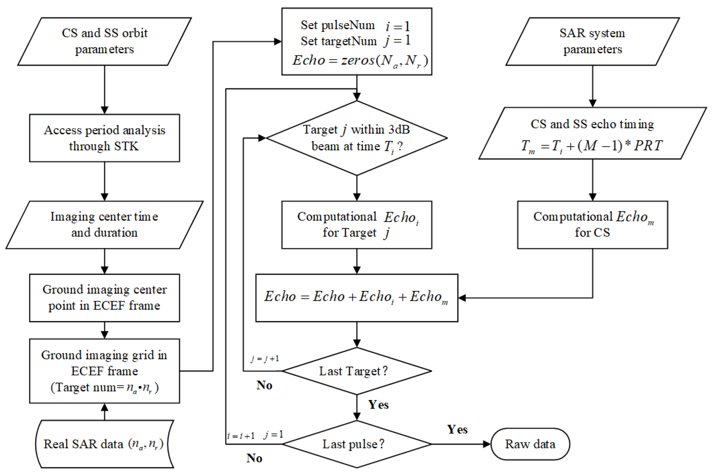
First, the accessible calibration period is analyzed using STK, based on the initial orbits of the CS and SS. The simulation center time and synthetic aperture time are then determined. A ground imaging grid in ECEF frame is then constructed by setting the scene center according to the orbital geometry. According to the timing analysis of CS and ground echoes in Section 2, and in combination with SAR system parameters, the slant range gate of the CS echo within each PRF frame is calculated, and the corresponding echo is superimposed onto the corresponding ground echo. To ensure the realism and reliability of the imaging simulation, ground echoes are generated using real SAR data as reference. Specifically, an already focused SAR image is used to provide amplitude information, replacing traditional scattering coefficient models. Random phases are added to each pixel to emulate realistic echo characteristics. The detailed simulation flowchart is illustrated in Figure 12 and the simulation parameters are detailed in

Table 6. Imaging simulation parameters.

Parameter	Value	Parameter	Value
SAR satellite	SS1	Radius of CS	0.25 m
Calibration satellite	CS1	SAR transmit power	2200 W
Radar wavelength	0.03125 m	Tx and Rx antenna gain	36.3 dB
Bandwidth	90 MHz	Receiver gain	20 dB
Sampling rate	100 MHz	System loss	1 dB
Pulse width	5 μs	Atmospheric loss	2 dB
Guard pulse width	0.5 μs	Side-looking offset angle	32°
Pulse repetition frequency	4500 Hz	Azimuth 3-dB beamwidth	0.2°
PulseNum	6750	Range 3-dB beamwidth	2°
SampleNum	6000	Azimuth resolution	2 m
CR range	774.038 km	CS range	7.886 km

.

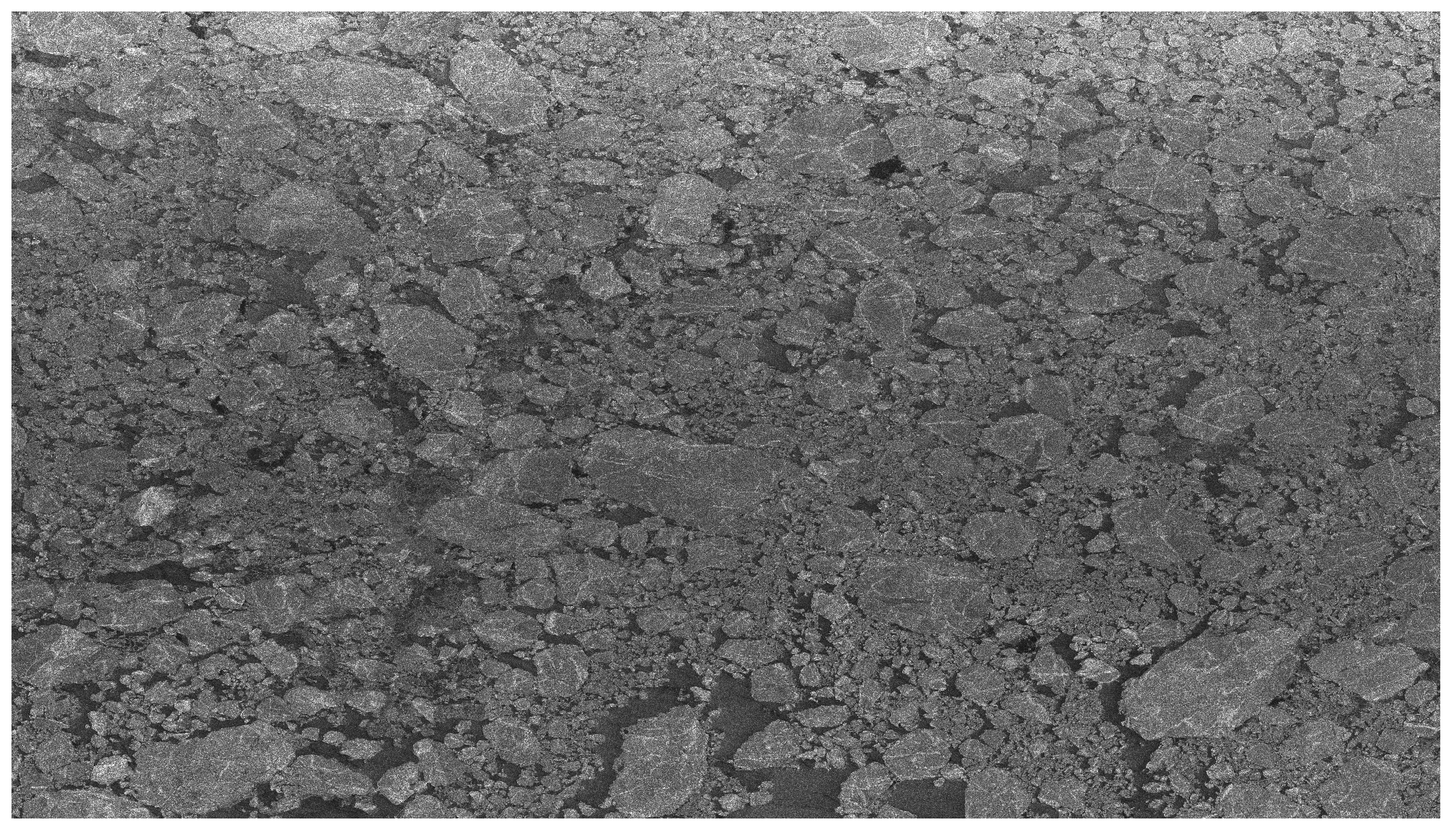
As analyzed previously, CS1 and SS1 operate in an elliptical formation with the same orbital period. The calibration is performed at the perigee ω = 90°, with sea ice imagery from the polar region near the North Pole selected as the reference scene, as illustrated in Figure 13.

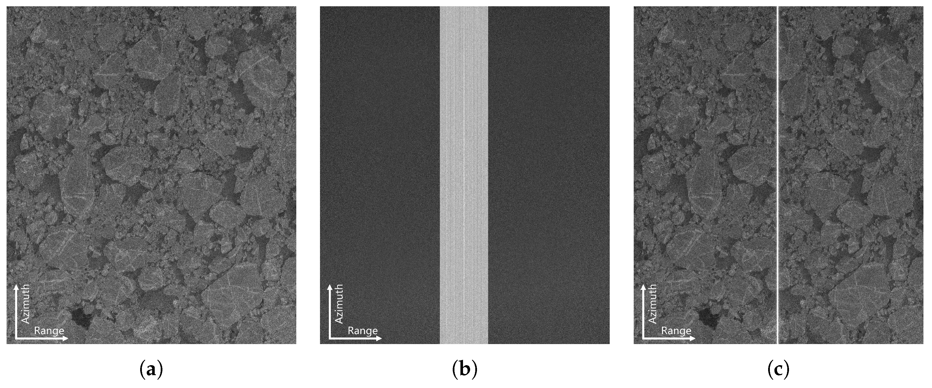
Following the simulation procedure illustrated in Figure 12 and the parameters specified in Table 6, imaging simulation experiments were carried out, and the results are summarized in Figure 14. Figure 14a shows the focused data of ground scene without the CS echo using the classical Chirp Scaling Algorithm (CSA). Raw data with superimposed CS echo and ground scene signal is illustrated Figure 14b, where the CS echo is much stronger than the ground scene signal. 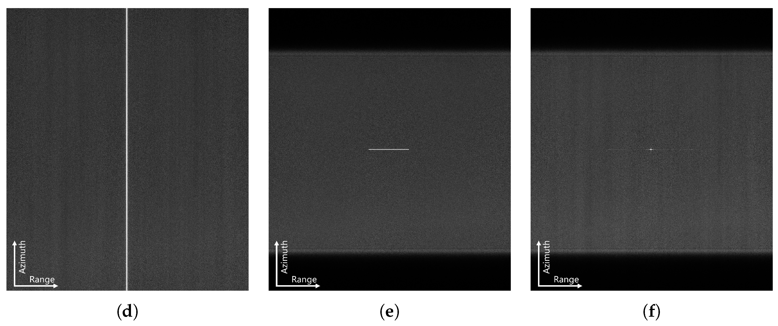Figure 14c shows the BP imaging result of the raw data in Figure 14b, displaying the focused ground scene signal. It can be observed that the ground scene remains well focused, while the CS, due to its strong echo energy and narrow Doppler bandwidth, appears as a bright stripe in the middle of the image, resembling the nadir echo. After applying range compression to the raw data, the time-domain image, depicted in Figure 14d, the CS echo focused at the right location with no range cell migration and ground scene signal focused at different ranges within the synthetic aperture. The range Doppler domain spectrum is obtained by performing a direct azimuth Fourier transform on the raw signal and is shown in Figure 14e and it can be observed that the energy of the CS is concentrated at only a few points in the range Doppler domain. Given that the frequency domain resolution is 4500/6750 = 0.6667 Hz and the Doppler bandwidth of the CS is approximately 2.1236 Hz, the expected number of occupied frequency bins is around 3, which is consistent with the discrete distribution observed in Figure 14e. Consequently, performing azimuth Fourier transform directly to the range-compressed data enables efficient focusing of the calibration satellite in the Range-Doppler domain as given in Figure 14f, and the CS energy can subsequently be extracted for radiometric calibration.

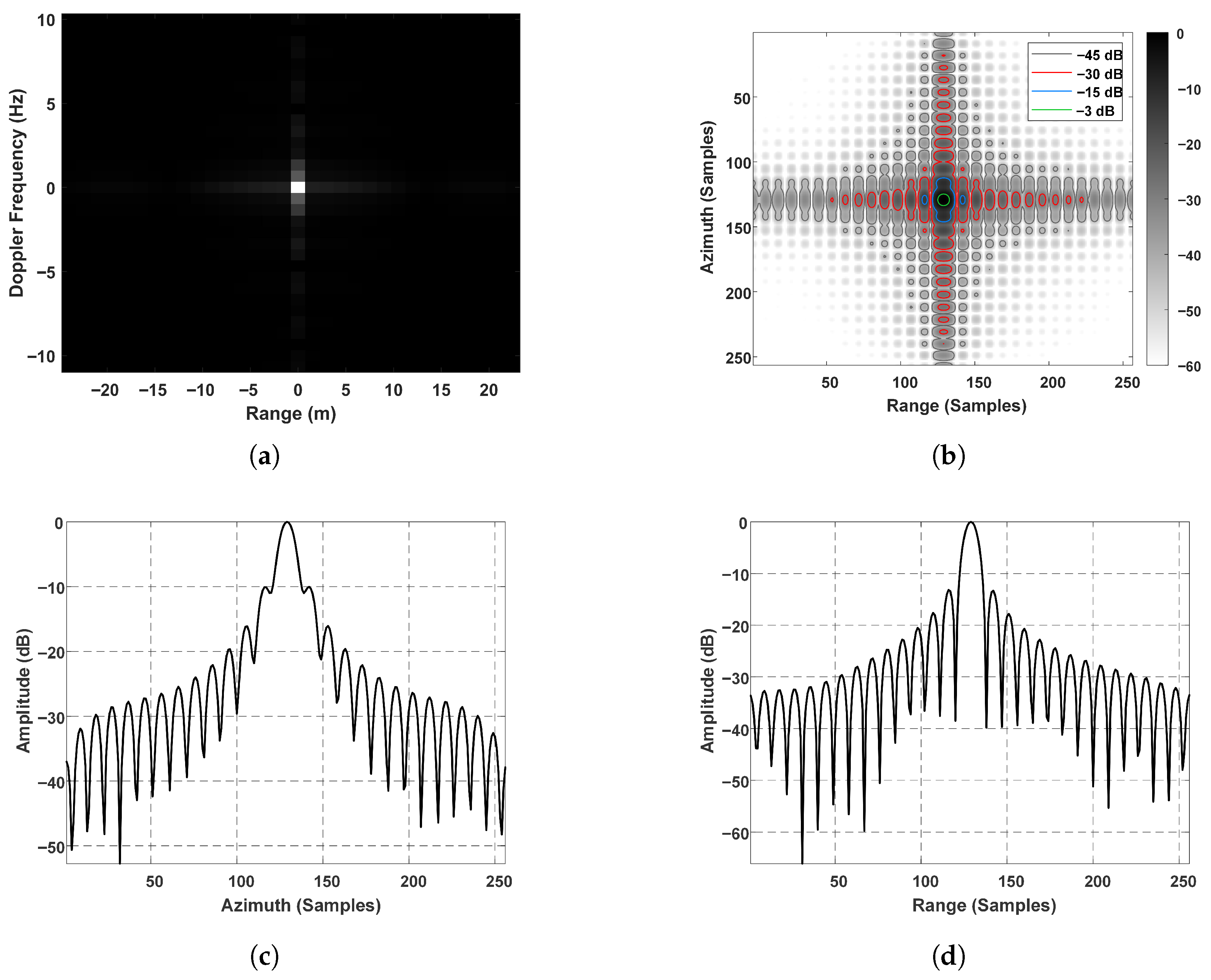
We extracted a 32 × 32 integration window data slice centered on the CS in Figure 14f and performed 8× upsampling on the slice. The focusing results of the CS after magnification and upsampling are shown in Figure 15. It can be observed that the CS is slightly defocused in the azimuth direction; however, the majority of its energy remains concentrated within the integration window as shown in Figure 15b, thereby having no significant impact on the accuracy of point target energy extraction.

The above results and analysis demonstrate the feasibility and effectiveness of using the CS to extract energy and compute the radiometric calibration factor. However, the CS differs significantly from ground targets in both imaging parameters and motion characteristics. As a result, using a ground-based SAR processor to handle its echoes often leads to poor focusing, making it difficult to extract CS energy.

Given the CS’s narrow Doppler bandwidth, small range cell migration, and strong echo strength, effective focusing can be achieved using only range compression and azimuth FFT. This simplified approach differs from the standard processing chain used by ground-based SAR systems.

Consequently, the calibration factor obtained through this method is not equivalent to that derived from SAR image processing of ground target. To align the results, a conversion must be performed that accounts for differences in imaging parameters and processing gain factors. A detailed analysis is presented in the next section.

5. Calculation and Transformation of Calibration Factor

In traditional SAR radiometric calibration, the system is often treated as a single “black box,” where the overall system gain is estimated by extracting the energy of point target responses from the focused SAR image. However, this process inherently couples the effects of both the radar hardware and the signal processor, making it difficult to distinguish their respective contributions to the calibration result. As a consequence, it is not possible to independently assess the radiometric performance of the radar system or the gain introduced by the signal processor.

Moreover, SAR image formation typically involves not only the basic two-dimensional matched filtering but also additional operations such as interpolation, resampling, and windowing. These steps introduce further processing gains or energy losses, which can affect the accuracy of point target energy extraction and ultimately degrade the precision of radiometric calibration.

In contrast, calibration using a dedicated calibration satellite (CS) offers distinct advantages. The CS signal processing chain is structurally simple and analytically tractable; as discussed earlier, only range compression and azimuth FFT are required to focus the signal and extract its energy, avoiding additional processing-induced distortions or losses. This enables effective isolation of radar system gain from signal processor gain, allowing a more accurate characterization of the intrinsic radiometric response of the SAR hardware. Based on this, a processor gain model or complementary ground-based calibration can be employed to convert the gain measured via the CS into a calibration factor applicable to actual SAR image products. As shown in Figure 16, this approach essentially deconstructs the SAR system “black box” into two separate subsystems—radar hardware and signal processor—so that their gain characteristics can be independently validated and evaluated, thereby enhancing the accuracy, transparency, and flexibility of the overall calibration process.

In this section we discuss the forms of the SAR radar equation which are appropriate for images of both ground point targets and the CS. Differences between calibration factors $K_g$ and $K_{cs}$ derived from ground point targets and CS are further analyzed, and transformation methods are provided.

5.1. Radar Equation for Ground Point Target

According to the (monostatic) radar equation, the expected power in a single pulse received from a ground reference point target of RCS, $\sigma$, at the raw data stage (i.e., after analog-to-digital conversion but prior to image formation processing) is calculated as Equation (5). Considering the additive (thermal) noise power $P_n$, the receiver output power $P_{r-g}$ (before any signal processing) can be expressed as follows:

$$P_{r-g}=C{\displaystyle \frac{1}{\lambda R^4{L}_a}}\sigma +P_n$$

(8)

where, for convenience, the SAR transmitter and receiver parameters are denoted as $C={\displaystyle \frac{P_t{G}_t^A\left({\theta }_{el},{\theta }_{az}\right)G_r^A\left({\theta }_{el},{\theta }_{az}\right)G_r^E{\lambda }^3}{{\left(4\pi \right)}^3{L}_s}}$, noting that significant errors in the SAR system hardware primarily stem from uncertainties in estimating C. Compared to SAR system hardware, the gain and errors of the signal processor are theoretically easier to model and quantify, as they are primarily determined by known algorithms and controllable parameters. However, during external calibration, any image deviations are difficult to attribute specifically to either processor or radar system errors when using point targets, which may compromise the accuracy of the calibration.

The image formation process, which fundamentally consists of azimuth and range compression operations performed on the digitized video signals, can be considered as a phase-compensated coherent integration and all other fundamental operations, such as forward and inverse FFTs, interpolation to correct range cell migration, etc., are assumed to be properly scaled. Since the echo signals from a point target are coherent and the noise components are random, the signal adds coherently in voltage, whereas the noise accumulates in power. Accordingly, the generalized radar equation for SAR correlation power $P_{r-g}^{\prime }$ is given by [35] (Freeman and Curlander, 1989):

$$P_{r-g}^{\prime }=C{\displaystyle \frac{1}{\lambda R^4{L}_a}}{N}^2{L}_w{N}_L\sigma +N{L}_w{N}_L{P}_n$$

(9)

where $N_L$ refers to the number of looks used in processing to suppress the speckle noise. $N=N_r·N_a$ is the number of samples integrated during the correlation processing and $L_w=L_{w_a}·L_{w_r}$ is the loss in peak signal strength due to azimuth and range reference function weighting. The parameters $N_r$ and $N_a$ are the range and azimuth reference function lengths and $L_{w_a}$, $L_{w_r}$ are the range and azimuth reference function weighting loss factors, respectively. For the SAR image that maintains the same azimuth resolution across the swath, the Doppler bandwidth should be constant, which implies that the azimuth correlation number $N_a$ is proportional to the slant range (R) and is expressed by the satellite ground speed ($V_g$), pulse repetition frequency ($PRF$), theoretical azimuth resolution (${\rho }_a$), and wave length ($\lambda$). The range correlation number $N_r$ is determined by the radar parameters, pulse duration (${\tau }_p$), and sampling frequency ($f_s$):

$$\left\{\begin{array}{cc}\hfill N_a& ={\displaystyle \frac{{\displaystyle \mathrm{PRF}}}{2V_g{\rho }_a}}\lambda R\hfill \\ \hfill N_r& ={\tau }_p{f}_s\hfill \end{array}\right.$$

(10)

In Equation (9), the signal power is inversely proportional to $R^2$ while the noise power increases linearly with R, since no normalization is applied to the reference function or the multilook filter to account for the number of integrated samples. To prevent the range-dependent increase in noise power, and to ensure that the noise statistics remain consistent across the image regardless of slant range, a relative calibration factor of

$$K_{rel}=\sqrt{N{L}_w{N}_L}$$

(11)

is required to normalize the reference function. Of course, while some studies use the normalization factor $K_a=\sqrt{N_a{L}_w{N}_L}$, either $K_a$ or $K_{rel}$ can be used to ensure slant-range-independent noise power, as both include the essential azimuth correction factor $N_a$. Assuming the normalization factor $K_{rel}$ is applied in Equation (11), the normalized power $\overline{P_{r-g}}$ for a point target is given as follows:

$$\begin{array}{cc}\hfill \overline{P_{r-g}}& =C·{\displaystyle \frac{1}{\lambda R^4{L}_a}}·N·\sigma +P_n\hfill \\ \hfill & =K_g\left(R\right)·\sigma +P_n\hfill \end{array}$$

(12)

Consequently, the noise is independent of range position within the image, which can be evaluated by operating the radar in a receive-only mode.

5.2. Radar Equation for Calibration Satellite

As discussed in Section 3, the echo from the calibration satellite (CS) is superimposed on the echo from a ground scatterer located at $R_0$, but the actual signal propagation distance corresponds to the distance between the SAR satellite (SS) and the CS, denoted as $R_{cs}$. Since the CS is located in orbital space, the signal does not pass through the atmosphere during the transmission and reception process. As a result, atmospheric propagation losses can be neglected. Therefore, the received power of CS before any signal processing is given by:

$$P_{r-cs}=C{\displaystyle \frac{1}{\lambda R_{cs}^4}}\sigma +P_n$$

(13)

In the CS signal processing workflow, the steps that contribute to processing gain are range compression and azimuth FFT. Due to the narrowband nature of the CS signal, its temporally extended waveform exhibits a spectrally concentrated representation in the frequency domain, where the total energy—preserved according to Parseval’s theorem—is effectively accumulated within only a few frequency bins. Therefore, the processed CS power in range Doppler domain (without windowing and FFT normalization) can be expressed as:

$$P_{r-cs}^{\prime }=C{\displaystyle \frac{1}{\lambda R_{cs}^4}}{N}_R^2{N}_A{N}_F\sigma +N_R{N}_F{P}_n$$

(14)

where $N_R$ is the range reference function lengths for the image that contain the CS, $N_A$ represents the number of samples integrated in azimuth (i.e., the number of PRIs that contain echoes from the CS) and $N_F$ is the FFT length. Similarly, we use the relative calibration factor $\sqrt{N_R{N}_F}$ to normalize Equation (14) and the radar equation for CS can be expressed as follows:

$$\begin{array}{cc}\hfill \overline{P_{r-cs}}& =C{\displaystyle \frac{1}{\lambda R_{cs}^4}}{N}_R{N}_A\sigma +P_n\hfill \\ \hfill & =K_{cs}\left(R\right)·\sigma +P_n\hfill \end{array}$$

(15)

The calibration factor $K_{cs}$ derived from the CS is inherently more representative of the intrinsic radiometric response of the SAR system for several key reasons.

First, as shown in Equation (15), the received signal power from the CS is determined solely by the radar system parameters (encapsulated in constant C), the propagation range $R_{cs}$ and the RCS $\sigma$ of the CS. Since the CS operates in space, atmospheric propagation losses are eliminated, reducing external uncertainties that would otherwise affect ground-based calibration targets.

Second, the signal processing chain applied to the CS echo is highly simplified, involving only range compression and azimuth FFT, both of which have well-defined and quantifiable processing gains. This simplicity allows the processed power to be accurately modeled and normalized, as in Equation (15), enabling the isolation of the radar system gain without interference from complex image formation operations such as interpolation, resampling, and windowing, which are typical in full SAR processing chains.

Consequently, the calibration factor $K_{cs}$ extracted from the CS observation predominantly reflects the true response of the SAR system’s transmit–receive chain and antenna characteristics, with minimal influence from the signal processor. This decoupling is particularly important because it allows system engineers to validate the hardware’s radiometric performance independently and more reliably, thereby improving both the traceability and accuracy of the overall calibration process.

5.3. Calibration Factor Transformation

As shown in the above derivation, although the calibration factor $K_{cs}$ obtained from the CS can accurately reflect the intrinsic radiometric response of the SAR system, it must still be converted to a form applicable to conventional SAR image products of ground scene. This necessity arises because the actual SAR image generation process typically involves a more complex imaging chain and different imaging parameters as analyzed before, which lead to discrepancies between the point target responses in the final image and those corresponding to the idealized CS scenario. Therefore, it is essential to establish an equivalent gain mapping between the two processing workflows by incorporating differences in imaging parameters. The ratio $K_g/K_{cs}$ in Equation (16) quantitatively captures the relative gain variation resulting from parameter and processing chain differences under identical radar system conditions. By evaluating this ratio, the calibration factor derived from the CS, $K_{cs}$, can be transformed into $K_g^{\prime }$, which is directly applicable to ground targets or SAR image products.

This conversion not only ensures consistency between the CS-based calibration and operational imaging scenarios but also enhances the traceability and interpretability of the radiometric calibration. Moreover, it enables a clear separation of radar system gain and signal processor gain effects, thereby supporting processor-independent performance verification and offering greater flexibility and generality for future SAR calibration strategies.

$$\begin{array}{cc}\hfill {\displaystyle \frac{K_g^{\prime }}{K_{cs}}}& ={\displaystyle \frac{1}{L_a}}·{\displaystyle \frac{N_r{N}_a}{N_R{N}_A}}·{\displaystyle \frac{R_{cs}^4}{R^4}}\hfill \end{array}$$

(16)

The atmospheric attenuation $L_a$ can be independently predicted using radar propagation models and treated as a separately correctable factor in the calibration process. Accordingly, the calibration factor $K_g^{\prime }$ applicable to ground point targets can be explicitly expressed as:

$$K_g^{\prime }=K_{cs}·{\displaystyle \frac{N_r{N}_a}{N_R{N}_A}}·{\left({\displaystyle \frac{R_{cs}}{R}}\right)}^4$$

(17)

This formulation accounts for differences in imaging parameters and processing chains between the calibration scenario and the actual SAR image generation. Moreover, considering $\sigma ={\sigma }_o{\rho }_a{\rho }_r/sin{\theta }_i$, the appropriate form of the calibration factor for a distributed target can be expressed as follows:

$$K_d^{\prime }=K_{cs}·{\displaystyle \frac{N_r{N}_a}{N_R{N}_A}}·{\left({\displaystyle \frac{R_{cs}}{R}}\right)}^4·{\displaystyle \frac{{\rho }_a{\rho }_r}{sin{\theta }_i}}$$

(18)

where ${\theta }_i$ is the incidence angle corresponding to the slant range R, and ${\rho }_a$ and ${\rho }_r$ are the resolution cell size after imaging processing.

6. Validation of Calibration Factor Transformation

To validate the proposed calibration factor transformation method—namely, converting the radiometric calibration factor $K_{cs}$ obtained from the CS into the calibration factor $K_g$ applicable to conventional SAR image products—a set of numerical simulation experiments was designed and conducted, as detailed in this section. The objective of the experiment is to verify the correctness and applicability of the gain ratio expression in Equation (16), which is used to compensate for the differences in imaging parameters between the calibration scenario and the conventional SAR imaging process.

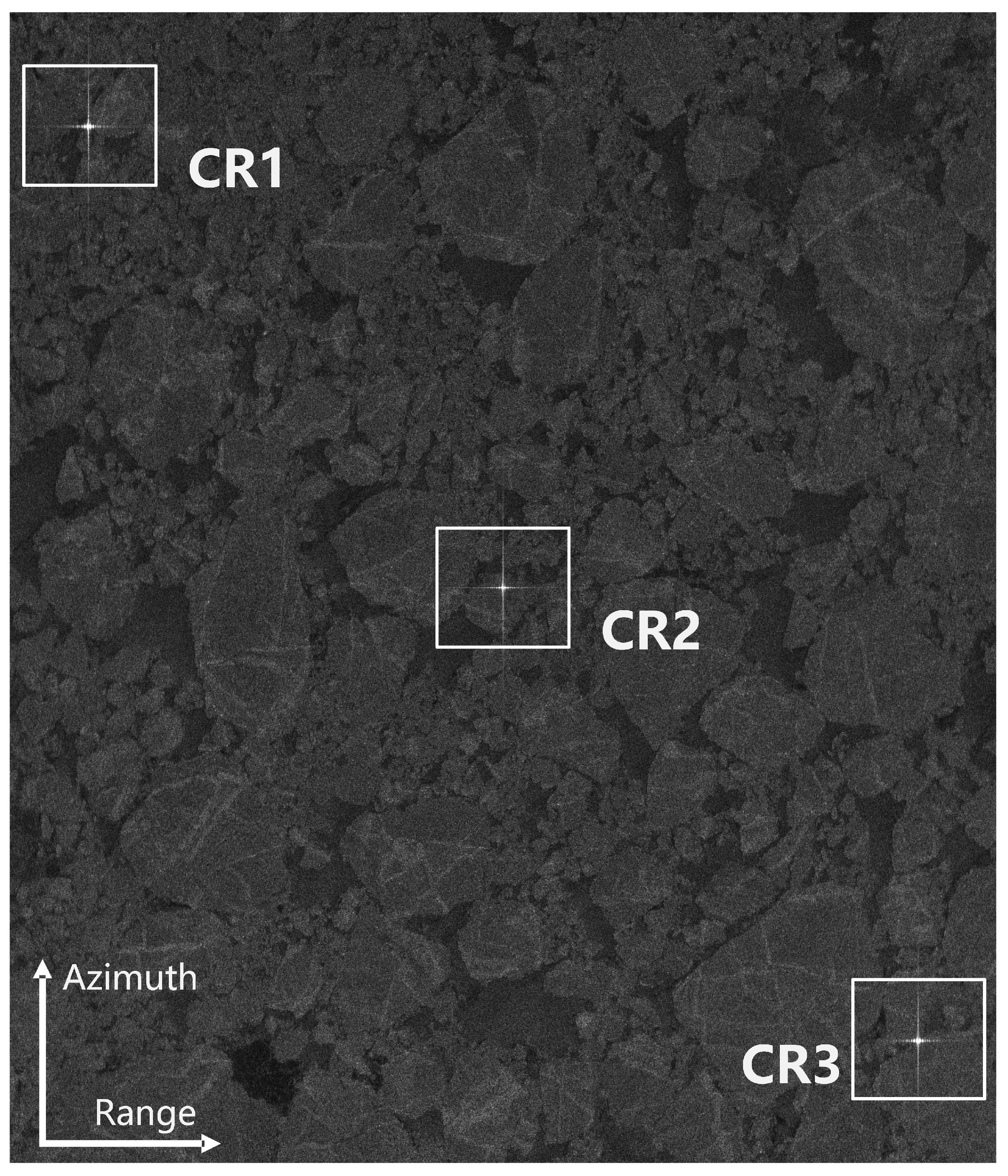
The simulation is based on the workflow outlined in Figure 12 and simulation parameters are shown in Table 6. Two SAR imaging scenarios are involved: (1) the calibration satellite scenario, and (2) the conventional ground scene scenario involving reference targets. Both simulations adopt identical radar system parameters, to ensure that the intrinsic radiometric characteristics of the radar system remain consistent. The key difference lies in the image processing parameters and processing chains.

In the calibration satellite scenario, system parameters follow the CS1 configuration, and the processing chain includes only range compression and azimuth FFT. In the ground SAR scenario, multiple reference targets with identical RCS values are uniformly distributed at different slant ranges. Image formation for the ground scenario employs the classical Chirp Scaling Algorithm. Relative radiometric correction has been completed, meaning the effects of the antenna pattern and slant range attenuation (normalized to the scene center range) have been compensated. The CS simulation results are shown in Figure 15 and the simulation results of ground scene is illustrated in Figure 17.

Energy extraction from the main lobe responses of both the CS and ground reference targets is performed using the integral method, based on which the calibration factors $K_{cs}$ and $K_g$ are calculated. Subsequently, Equation (16) along with the relevant imaging parameters is used to convert $K_{cs}$ into the transforming calibration factor $K_g^{\prime }$, which is then compared with the $K_g$ directly derived from ground targets for validation. The response energy and calibration factor results of ground reference targets and CS are illustrated in

Table 7. Response energy and calibration factor results for CS and ground reference targets.

Target ID	RCS (dBsm)	Response Energy (dB)	Calibration Factor (dB)	Factor After Transformation
CR1	43.4	−35.5524	−78.9524	–
CR2	43.4	−35.5773	−78.9773	–
CR3	43.4	−35.5631	−78.9631	–
CS1	−7.08	−6.3865	0.6935	−78.9820

.

As shown in the table, due to differences in imaging parameters and processing chain, the calibration factor $K_{cs}$ obtained from the CS differs significantly from the calibration factor $K_g$ derived from ground point target, making it unsuitable for direct use in radiometric calibration of ground SAR images. In contrast, the converted calibration factor $K_g^{\prime }$ closely matches that computed from ground point targets, demonstrating the effectiveness of the proposed calibration measurement and conversion method based on the calibration satellite.

7. Discussion

This work investigates the use of a calibration satellite as a space-based reference target, and provides a detailed analysis accordingly. For practical payload selection, two options are available—both of which have been extensively used in other fields, such as ground-based surveillance radar RCS calibration and atmospheric density measurement, demonstrating their technical maturity. The first option is a passive metal calibration sphere, consisting only of a hollow aluminum shell with no additional satellite components. It serves purely as a reflective target in orbit and lacks attitude and orbit control capabilities. Advantages include simple structure, no electromagnetic interference, and low cost; however, their inability to maintain orbit limits them to short-term calibration missions. Widely used calibration metal spheres include LCS, Calsphere, and POPCAS [15,16,17], with diameters typically ranging from 0.1 m to 1 m. These targets are characterized by exceptional radiometric stability. A prime example is LCS-4, which has served as a reliable calibration standard for ground-based surveillance radars since its launch in 1971, exhibiting negligible RCS variation over more than five decades. The second option is maneuverable calibration satellites equipped with isolated targets. These satellites carry calibration payloads (metal spheres or Luneberg lens) and additional components like solar panels, gyroscopes, and onboard processors, enabling both attitude and orbit control, enabling long-term calibration missions. During calibration, the payload is continuously oriented toward the target device, effectively shielding it from electromagnetic interference caused by other satellite structures. Representative examples are the Tianping-1 satellite [19] and a concept proposed in [22].

Traditional ground-based radiometric calibration requires relatively clean calibration sites with flat terrain, homogeneous surface coverage, and low, stable background scattering to reduce background clutter interference and improve the signal-to-clutter ratio. However, due to the relatively short distance between the calibration satellite and the SAR satellite, the echo from the calibration satellite is significantly stronger and exhibits a much higher SCR than typical ground targets. Moreover, the echoes propagate exclusively through the space environment, avoiding common ground-based interferences such as multipath effects. Under these conditions, the influence of ground background on calibration accuracy is substantially reduced. Therefore, space-based calibration does not rely on strict site selection, greatly enhancing the flexibility and applicability of the calibration process.

Although the CS periodically passes through the SAR antenna beam, it does not interfere with the SAR satellite’s routine Earth observation tasks. This can be ensured through the following two measures: First, by appropriate orbital design, the nadir points of both satellites during the calibration opportunities are positioned over non-priority observation regions (e.g., polar areas), thereby avoiding overlap with key imaging zones. In other words, the CS is only visible to the SAR system within the designated high-latitude regions, and remains outside the beam coverage at other latitudes. Second, effective isolation between calibration and imaging signals can be achieved through dedicated beam arrangement design and SS-To-CS distance control. As analyzed in Section 3, the SS-to-CS distance must satisfy specific constraints for CS echoes to align with the radar timing of the existing beam arrangement. Leveraging this characteristic, the orbit formation size and SS-To-CS distance are deliberately configured to ensure that the CS echoes fall outside the radar timing window of the existing beam arrangement, thus preventing their reception during routine SAR imaging. Furthermore, a dedicated calibration beam can be designed with a tailored reception window that avoids ground echoes and exclusively receives the CS echoes. This enhances signal isolation, improves the signal-to-clutter ratio (SCR), and enables high-precision characterization of the radar system. These two strategies will be further explored and refined in our future work to enhance the compatibility between calibration operations and routine SAR imaging tasks.

In addition to the above system-level considerations, several practical error sources may affect the calibration performance. Orbit errors may introduce slant-range uncertainties, which propagate into the radiometric calibration through the range normalization process. Since the resulting bias is governed by the relative slant-range error, and the sensor-to-target distance is typically much larger than the orbit determination error, the induced radiometric impact is expected to be very small and not a dominant factor. Attitude errors mainly manifest as beam alignment errors between the calibration satellite and the SAR system. Their impact depends on the angular response of the calibration target: antenna-based devices are constrained by the antenna beamwidth, whereas passive reflectors are governed by the angular width of the scattering response. In general, a wider angular response provides greater robustness against pointing inaccuracies. Timing errors may lead to a mismatch between the predicted echo arrival time and the SAR receiving window, thereby affecting echo capture and subsequent energy extraction; however, this effect can be effectively mitigated through accurate orbit prediction and proper scheduling of SAR operations. Finally, for passive calibration devices such as metal spheres, the uncertainty in the calibration-target radar cross section (RCS) is typically limited, as demonstrated by their high long-term stability in previous missions, and is therefore not expected to be a dominant factor affecting the feasibility of the proposed method. For active calibration satellites, maintaining the long-term accuracy of onboard calibration payloads remains an important issue; however, this problem is related to the in-orbit characterization of the calibration device itself and lies beyond the scope of the system-level framework addressed in this paper.

Three representative calibration scenarios and corresponding orbit selection strategies are presented. Future research will systematically incorporate mission-specific constraints such as calibration frequency, multi-beam calibration requirements, and long-term formation stability, along with realistic satellite parameters and perturbation models, to conduct optimized orbit configuration design tailored to specific mission objectives, thereby enhancing the practicality and robustness of the calibration system.

8. Conclusions

This paper presents a novel space-based approach for the absolute radiometric calibration of spaceborne SAR systems using a small calibration satellite (CS). The proposed method effectively overcomes the limitations of traditional ground-based calibration techniques, which are often costly, time-consuming, and restricted by geographical and atmospheric conditions. By deploying a CS equipped with well-characterized calibration devices, such as passive reflectors or active transponders, in a carefully designed orbital formation, the SAR satellite (SS) can periodically image the CS to derive accurate calibration factors to evaluate the radar system. Furthermore, by examining the differences between the imaging parameters and processing chains of the CS and ground scene images, the calibration factor derived from the CS can be appropriately transformed to ensure its applicability to ground imaging products.

The key advantages of this method include:

• Independence from ground calibration site: The fully space-based calibration approach eliminates the influence of atmospheric and ionospheric effects, as well as ground clutter and multipath interference.
• Enhanced Flexibility and Calibration Frequency: The calibration satellite can facilitate frequent calibrations for one or multiple SAR satellites operating in various orbital configurations, greatly improving calibration availability and adaptability.
• Improved Radiometric Accuracy: The simplified echo signal processing chain in the CS scenario allows for precise separation of radar system gain and signal processor gain, resulting in more accurate and reliable radiometric calibration compared to traditional ground-based methods.

The feasibility of this approach has been validated through orbital simulations, imaging analysis, and calibration factor conversion experiments. The results show that the calibration factors derived from the CS can be accurately transformed for application to ground-based SAR image products, ensuring consistency and reliability.

Moreover, this calibration method is not only applicable to Earth-orbiting SAR missions but also shows great potential for deep space exploration scenarios, where traditional calibration methods are infeasible. Future work will focus on optimizing orbital configurations for multi-satellite calibration and further refining transformation models to enhance accuracy and applicability.

In summary, the proposed approach marks a significant advancement in SAR radiometric calibration, offering a robust, flexible, and scalable solution for both current and next-generation SAR missions.