Forecasting Sea Surface Cooling During Typhoons Based on Machine Learning

Highlights

What are the main findings?

• The MLP-based prediction model for sea surface cooling (SSC) during typhoons performed well across 46 typhoon cases in the Northwest Pacific, achieving high prediction accuracy.
• The model reproduced the classic rightward-biased asymmetry in SSC spatial distribution and captured the nonlinear relationship between typhoon dynamic forcing and ocean thermal response. Analysis shows that SSC is influenced by ocean thermal structure, mesoscale eddies, and typhoon dynamic characteristics, with feature importance analysis identifying the key predictors and their directional effects.

What are the implications of the main findings?

• The MLP model developed in this study offers a new, efficient method for predicting SSC during typhoons. It requires only a few key inputs to make reliable predictions, providing a practical technical solution for developing marine environment forecasting tools.
• This study reveals how typhoon-induced SSC is jointly influenced by the ocean’s initial thermal structure, mesoscale eddies, and typhoon dynamic characteristics. The findings can support marine disaster risk assessment, coastal disaster prevention, marine aquaculture, ecosystem protection, and help improve mixed-layer parameterization in operational coupled ocean-atmosphere models.

Abstract

Sea surface cooling (SSC) induced by typhoons has a significant impact on typhoon intensity and regional air–sea interaction. This study develops a machine learning model based on a multilayer perceptron (MLP) to predict SSC during typhoon passage over the western North Pacific. The model uses pre-typhoon ocean background conditions and ocean states at the typhoon peak moment as inputs, including wind field, sea level anomaly (SLA), mixed layer depth (MLD), and 100 m water temperature. Trained on historical typhoon data and multi-source ocean observations from 2002 to 2018, the model directly predicts SSC during typhoon events from 2019 to 2020. Results show that the model achieves a mean absolute error (MAE) of 0.379 °C, a root mean square error (RMSE) of 0.488 °C, and a bias of 0.087 °C. The model reproduces the typical rightward bias in SSC spatial distribution. Under normal ocean conditions, such as open deep-water areas with moderate stratification and no strong eddy interference, the model performs well, with errors below 0.1 °C at some points. Although some biases exist under complex ocean environments and abrupt changes in typhoon dynamics, the model still captures the overall cooling trend. This study demonstrates the feasibility of machine learning for typhoon–ocean interaction forecasting. The proposed framework can provide technical support for typhoon intensity forecasting, marine disaster warning, and aquaculture risk prevention.

1. Introduction

Tropical cyclones (TCs) are mesoscale weather systems that form over warm oceans. In the Northwest Pacific, they are called typhoons. As one of the most destructive natural disasters, typhoons bring strong winds, heavy rain, and storm surges that threaten coastal areas. When a typhoon passes over the ocean, its low central pressure and strong wind stress cause intense mixing and divergence between the upper and lower ocean layers. The strong winds deepen the mixed layer through entrainment and drive upwelling, which redistributes surface waters and leaves a cold trace in the upper ocean—a drop in sea surface temperature (SST), known as sea surface cooling (SSC) [1,2,3]. The cooling typically ranges from 1 to 6 °C [4] and can exceed 10 °C in extreme cases [5,6]. This SSC reduces the heat flux from the ocean to the atmosphere, weakening the typhoon and creating a negative feedback loop [7,8,9,10,11]. In the Northern Hemisphere, the largest cooling usually occurs to the right of the typhoon track [12,13,14]. The magnitude and extent of SSC are closely related not only to typhoon intensity and translation speed, but also to ocean background conditions [13,15,16,17,18,19]. In addition to SSC, typhoon-induced mixing and upwelling bring nutrients to the surface and cause rapid temperature changes, which affect marine ecosystems and coastal aquaculture [20,21,22]. Therefore, it is important to study how the ocean responds to typhoons, identify the key mechanisms involved, and improve typhoon forecasting and coastal fishery risk management.

Because of the importance of SSC, researchers have developed fully coupled air–sea models for typhoon prediction [23,24,25,26]. These models can simulate typhoon-induced SSC [27,28,29,30,31], but they are built on physical equations and numerical methods, which introduce uncertainties and high computational costs. In recent years, machine learning has offered new ways to study typhoon–ocean interactions. In existing machine learning studies on SSC, one common approach treats typhoon passage as a time series prediction problem, using step-by-step inputs to track SST changes over time. Zhang et al. [32] used an LSTM network to predict SST six hours ahead, based on current 10 m wind speed, sea surface height (SSH), SST, and 100 m water temperature. Shao et al. [33] combined empirical orthogonal function decomposition with a Conv1D-LSTM model, using time series of sea surface height anomaly (SSHA) and SST to predict SST changes in the South China Sea under typhoon conditions. Their model captured the cooling trend, although the cooling amplitude was slightly lower than observed, and it performed better than persistence forecasts and linear regression.

Another approach avoids iteration by directly mapping input features to output results. Zhao et al. [34] built a deep learning model (RC_ViT) that combines a residual CNN, ConvLSTM, and Vision Transformer. It takes the SST field of the past seven days, forcing wind fields, topography, current time, and target time as inputs, and directly predicts the SST distribution one day ahead to forecast the typhoon cold wake. Cui et al. [16] used a random forest method with 12 predictors, including typhoon characteristics and pre-storm ocean conditions, to predict SST anomalies from three days before to 14 days after a typhoon passes. These methods can directly output SST fields for several days, but they require post-processing to obtain cooling values.

Different from the above methods, some researchers have tried to predict cooling directly. Wei et al. [35] developed a three-layer neural network that takes wind speed, sea surface height, SST, and subsurface water temperature as inputs and directly outputs SSC, feeding it back to the WRF typhoon model. This approach made the typhoon intensity simulated by WRF close to that of the WRF-ROMS coupled model and avoided the overestimation caused by fixed SST. Jiang et al. [36] proposed shallow-learning and deep-learning neural network schemes using a layered neuron matrix. Their method reduced the MAE of maximum wind speed in the WRF model by 60–77% and the MAE of SST to 0.57–0.77 °C. These methods avoid error propagation, are computationally efficient, and can be embedded in atmospheric models for real-time feedback.

These studies have opened new avenues for understanding and predicting typhoon-induced SSC. However, most existing studies use either instantaneous values at a certain time, historical time series, or average conditions before or during typhoon passage. Although these inputs reflect the overall intensity of the typhoon, they cannot accurately capture the strongest instantaneous forcing that acts on the sea surface during the typhoon. Even when a study used the maximum wind speed [29], it only used that single value without also extracting other ocean variables at the same time. In fact, the key dynamic and thermal conditions that drive the core cooling processes—vertical mixing, entrainment, and upwelling—usually correspond to an extreme forcing state at a specific time in the typhoon’s life cycle: the “peak perturbation” of the ocean by the typhoon. The wind stress, sea surface height anomaly, and subsurface thermal structure at that moment directly determine the magnitude and spatial distribution of the subsequent SSC. None of the previous studies used this set of peak-moment variables as model input, which is a gap in current research.

To address this gap, this study builds an MLP-based model to predict SSC during typhoons. In terms of feature selection, the model introduces instantaneous variables at the moment of maximum composite wind speed during the typhoon. Here, the “moment of maximum composite wind speed” is defined as the time when the composite wind speed, $\sqrt{u^2+v^2}$, reaches its maximum at a given grid point during the typhoon’s passage. The model combines these peak-moment variables with pre-typhoon background ocean conditions as inputs to directly output SSC. Compared with indirect methods that first predict SST and then compute cooling, direct prediction avoids error accumulation from two-step calculations and improves prediction accuracy. The model is trained on typhoon and multi-source ocean data from 2002 to 2018 and independently tested on typhoon cases from 2019 to 2020. To evaluate the model’s interpretability and its performance in different ocean environments, this study compares the model predictions with observations from multiple perspectives, including the spatial distribution of cooling, along-track and cross-track profile structures, vertical ocean stratification, and the modulation effects of mesoscale eddies.

The rest of this paper is organized as follows. Section 2 describes the data and methods used in this study. Section 3 presents the model predictions, overall performance, typical case analyses, and error analysis. Section 4 and Section 5 contain the discussion and conclusions.

2. Data and Methods

2.1. Multi-Source Satellite Remote Sensing Data

This study takes the Northwest Pacific (north of the equator to 60°N, 100°E to 180°E) as the core research area, and uses satellite remote sensing and reanalysis data products to comprehensively analyze the response of the upper ocean of the Northwest Pacific to tropical cyclones. The specific information of all data is shown in Table 1.

Table 1. Multi-source data products information.

Data Type	Product Name	Source Institution	Temporal Resolution	Spatial Resolution
Tropical Cyclone Data	Satellite Analysis Tropical Cyclone Scale Dataset (Version 3.0)	Shanghai Typhoon Institute, China Meteorological Administration	6-hourly	-
Sea Surface Temperature	MW_IR Optimal Interpolation (OI) Daily SST	Remote Sensing Systems	Daily	~9 km
Sea Surface Wind	Cross-Calibrated Multi-Platform (CCMP) v3.1	Remote Sensing Systems	6-hourly	0.25° × 0.25°
Sea Level Anomaly	SEALEVEL_GLO_PHY_L4_MY_008_047 (DUACS)	Copernicus Marine Service	Daily	0.125° × 0.125°
Ocean Temperature	GLOBAL_MULTIYEAR_PHY_001_030 (GLORYS12V1)	Copernicus Marine Service	Daily	0.083° × 0.083°
Mixed Layer Depth

2.2. Feature Selection and Extraction

To determine the typhoon influence period for each grid point, this study uses the radius of 8-level winds (wind speed ≥ 17.2 m/s) as the criterion. The dynamic influence area of each typhoon is defined by averaging the 8-level wind radii in four directions. For any affected point, the start time $t_s$ is recorded when the 8-level wind circle first covers the point, and the end time $t_e$ is recorded when the wind circle leaves the point (wind speed < 17.2 m/s). According to previous studies, SST along the typhoon path begins to respond 1–5 days before the typhoon arrives [18,27,37]. Therefore, the ocean conditions 5 days before the typhoon are taken as the stable background state.

SSC is essentially the result of dynamic forcing and thermal response. Previous studies have shown that the magnitude and spatial distribution of SSC are mainly controlled by two factors: the intensity of typhoon forcing, and the initial thermal and dynamic state of the ocean. Based on this, this study adopts commonly used feature variables from existing machine learning studies [32,35,36,38], including wind field, sea level anomaly (SLA), mixed layer depth (MLD), and ocean temperature at 100 m depth while adding background and peak timing information to capture the key physical processes controlling SSC.

The average value of each variable over the 5 days before $t_s$ is taken as the pre-typhoon background state, representing the initial ocean conditions. Among these, zonal wind (uwnd_0) and meridional wind (vwnd_0) represent the initial disturbance of the background wind field on the upper ocean; sea level anomaly (sla_0) reflects the distribution and intensity of background mesoscale eddy activity; mixed layer depth (mld_0) determines the heat capacity of the upper ocean and is a key thermal parameter regulating SSC; and ocean temperature at 100 m depth (t100_0) represents the subsurface thermal reserve. According to Price [39], the typical depth of vertical mixing for a strong typhoon is about 100 m. Therefore, this depth is a key layer for evaluating the impact of typhoons on the upper ocean thermal structure.

During the period $[t_s,t_e]$, the moment when the composite wind speed $\sqrt{u^2+v^2}$ reaches its maximum is identified, and the instantaneous variable values at that moment are extracted. The peak moment is chosen rather than the average state during the typhoon passage because the key dynamic conditions driving vertical mixing, entrainment, and upwelling often correspond to the strongest disturbance exerted by the typhoon on the ocean. The wind stress input at this moment directly determines the magnitude and spatial distribution of the subsequent SSC. Here, zonal wind (uwnd_max) and meridional wind (vwnd_max) represent the direct forcing driving vertical mixing and upwelling; sea level anomaly (sla_wsmax) reflects the local dynamic response of the sea surface at the peak forcing moment and is related to the modulation effect of mesoscale eddies; and ocean temperature at 100 m depth (t100_wsmax) represents the subsurface thermal condition at the peak forcing moment. The physical meanings of all features are summarized in Table 2.

Table 2. Summary of input features used in the MLP model.

Feature	Unit	Temporal Definition	Physical Meaning
uwnd_0, vwnd_0	m/s	Average of 5 days before $t_s$	Background wind stress
sla_0	m	Average of 5 days before $t_s$	Background mesoscale eddy activity
mld_0	m	Average of 5 days before $t_s$	Upper ocean heat capacity and stratification
t100_0	°C	Average of 5 days before $t_s$	Subsurface thermal reserve
uwnd_max, vwnd_max	m/s	At peak composite wind speed moment	Peak wind stress forcing
sla_wsmax	m	At peak composite wind speed moment	Peak dynamic height anomaly
t100_wsmax	°C	At peak composite wind speed moment	Subsurface thermal condition during peak forcing

Combining the background ocean state with the peak-stage variables captures both the initial thermal reserve of the ocean and the dynamic forcing of the typhoon. This combination provides a more complete description of the typhoon–ocean interaction process and helps improve prediction reliability.

2.3. Target Variable Definition

The prediction target of this study is SSC. Following previous studies [40], SSC is defined as the difference between the pre-typhoon background SST ($SS{T}_0$) and the minimum SST during and after the typhoon passage ($SS{T}_t$).

First, we calculate the background SST at a given point before the typhoon arrives ($SS{T}_0$). $SS{T}_0$ is the average SST over the five days before $t_s$:

$$SS{T}_0=({SST}_{t_s-1}+{SST}_{t_s-2}+{SST}_{t_s-3}+{SST}_{t_s-4}+{SST}_{t_s-5})/5,$$

(1)

Since most significant cooling occurs within 5 days after typhoon passage [41], $SS{T}_t$ is defined as the minimum SST from $t_s$ to 5 days after $t_e$:

$$SS{T}_t=\min \left(SS{T}_{t_s},{SST}_{t_s+1},\dots ,SS{T}_{t_e},\dots ,{SST}_{t_e+5}\right),$$

(2)

Finally, SSC is calculated as:

$$SSC=SS{T}_0-SS{T}_t,$$

(3)

2.4. Data Preprocessing

We first preprocessed the data as follows. Outliers were removed using statistical methods. Missing values were filled with the K-Nearest Neighbors (KNN) algorithm, and noise was reduced by filtering. The typhoon and ocean data were then matched by typhoon number and time stamp, and interpolated to a spatial grid of 0.25° × 0.25° with a 6 h time resolution. For each typhoon, the average radius of 8-level winds was used to define its influence range, and the corresponding parameters were extracted to build a typhoon–ocean dataset. To remove the effect of different units, all input features were normalized using Z-score standardization, so that each feature has a mean of 0 and a standard deviation of 1. The data were split into a training set and a test set. The training set includes 410 typhoons from 2002 to 2018, with 371,359 valid grid samples. The test set includes 46 typhoons from 2019 to 2020, with 33,947 valid grid samples.

2.5. Model Construction and Training

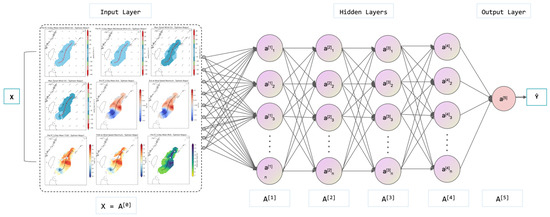
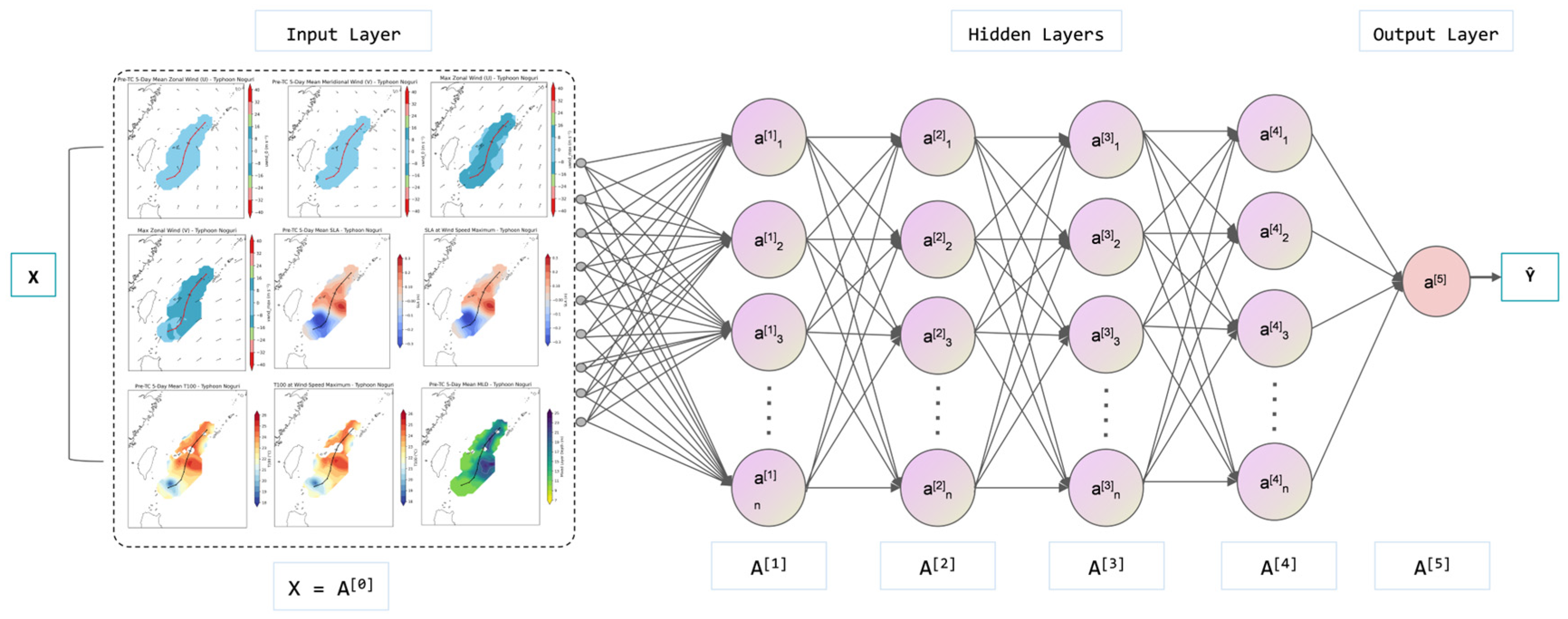
MLP is a feedforward neural network with strong nonlinear fitting ability. It consists of an input layer, several hidden layers, and an output layer. Layers are fully connected through learnable weight matrices. We used grid search to tune the hyperparameters, including the number of hidden layers, the number of neurons in each layer, and regularization parameters (dropout rate and L2 regularization strength). The optimal configuration had 4 hidden layers with 256, 128, 64, and 32 neurons, respectively. The L2 regularization coefficient was set to 0.001, and the dropout rates were 0.2 for the first three hidden layers and 0.1 for the last one. The structure of the MLP model is shown in Figure 1. The input layer has 9 neurons, corresponding to the 9 input features extracted in Section 2.2 (five background variables and four peak-forcing variables).

Figure 1. Schematic diagram of the MLP model architecture.

During forward propagation, the input data go through the input layer, then pass through a series of linear operations (weights $W$ and biases $b$) and activation functions in the hidden layers. The data finally reach the output layer to produce the predicted value. For any layer $l$, the output of a neuron is given by:

$$z^{\left(l\right)}=W^{\left(l\right)}{a}^{\left(l-1\right)}+b^{\left(l\right)},$$

(4)

$$a^{\left(l\right)}=f\left(z^{\left(l\right)}\right),$$

(5)

where $W^{\left(l\right)}$ and $b^{\left(l\right)}$ are the weight matrix and bias vector of layer $l$, $f$ is the activation function, and $a^{\left(l\right)}$ is the output of layer $l$, which also serves as the input to layer $l+1$.

All hidden layers use the Rectified Linear Unit (ReLU) as the activation function. Batch normalization is applied to speed up training. The model is optimized using the Adam algorithm with an initial learning rate of 0.001. During training, 10% of the training set is randomly selected as a validation set to monitor the training process. An early stopping strategy is used to prevent overfitting: if the validation loss does not decrease for 6 consecutive epochs, the learning rate is halved; if it does not improve for 12 consecutive epochs, training is stopped early and the network weights with the lowest validation loss are restored.

2.6. Feature Importance Analysis

To improve model interpretability, we used SHAP (SHapley Additive exPlanations) to analyze the importance of each input feature. SHAP is based on the Shapley value from game theory. It breaks down the model’s prediction into contributions from each feature:

$$f\left(X_i\right)=E\left[f\left(x\right)\right]+{\varphi }_1+{\varphi }_2+\cdots +{\varphi }_n,$$

(6)

Here, $f\left(x\right)$ is the predicted value, $X$ is the input feature, and $E\left[f\left(x\right)\right]$ is the average prediction across all samples. ${\varphi }_i$ represents the contribution of each feature to the prediction. A positive value means the feature increases the predicted SSC, and a negative value means it decreases it.

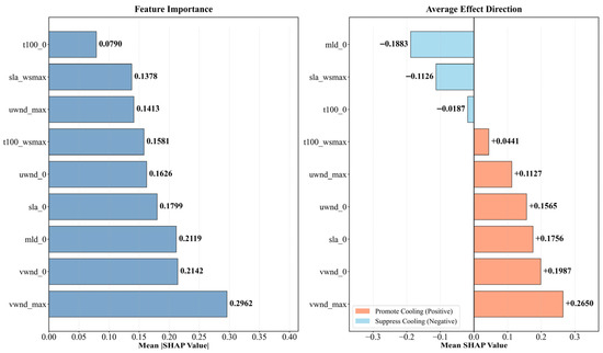
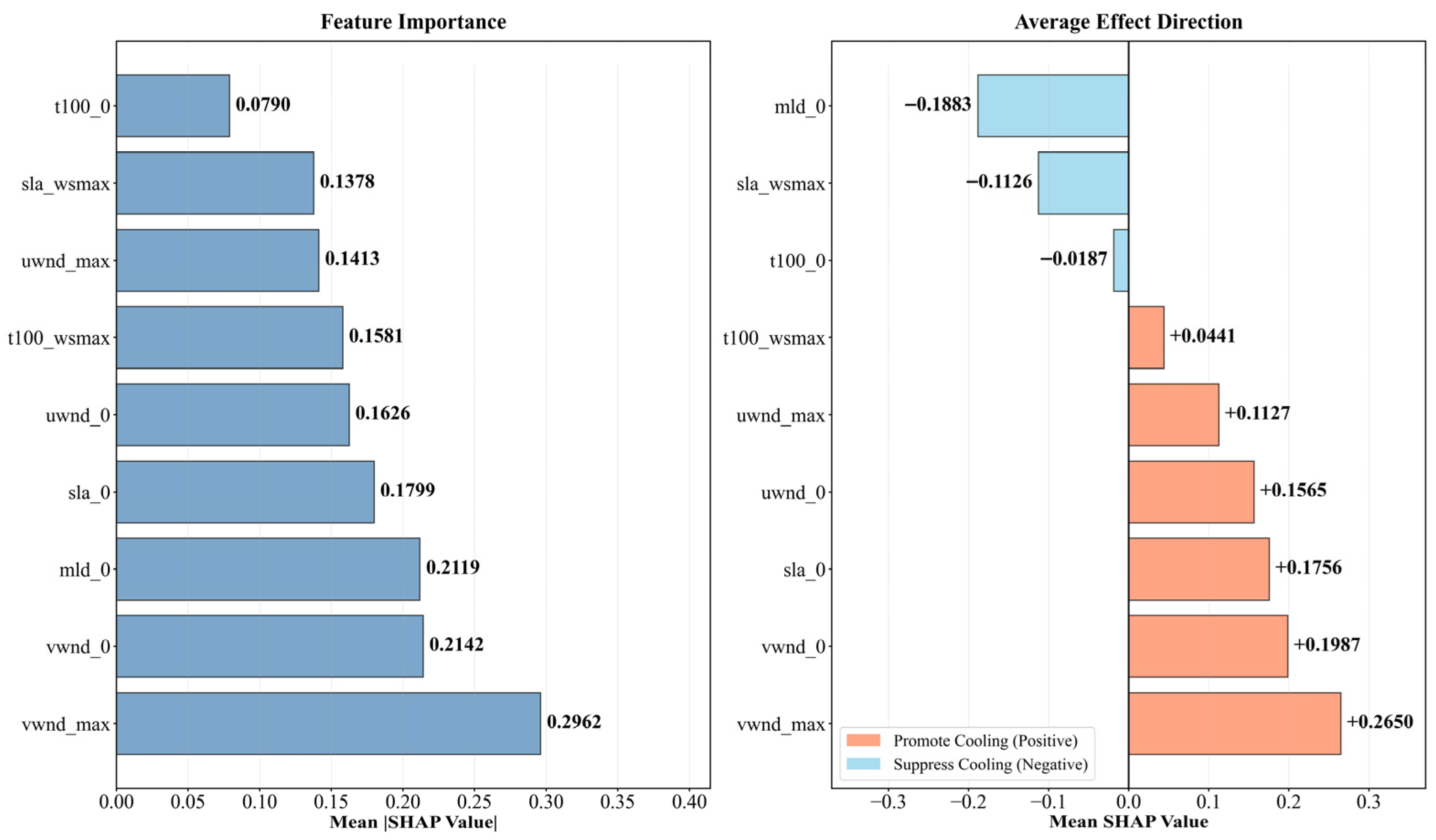
As shown in Figure 2, the meridional wind variables (vwnd_max, vwnd_0) and the initial mixed layer depth (mld_0) have the strongest influence on the prediction. This confirms that including wind speed at the peak forcing moment plays a key role in the model. In terms of impact direction, mld_0, sla_wsmax, and t100_0 have negative SHAP values. This means that higher values of these features lead to lower SSC predictions, meaning they suppress cooling. All other features have positive SHAP values and promote cooling. The meridional wind variables (vwnd_max, vwnd_0) have a stronger impact than the zonal wind variables (uwnd_max, uwnd_0). This suggests that meridional wind plays a more important role in ocean responses in this region.

Figure 2. Summary of Feature Importance.

A negative SHAP value for mld_0 means it suppresses cooling. This matches the common understanding that a shallow mixed layer favors cooling. In terms of ocean thermal conditions, t100_wsmax has a positive effect (promotes cooling), while t100_0 has a negative effect (suppresses cooling). This opposite behavior shows that the ocean thermal state has a nonlinear effect on SSC. When wind speed exceeds a certain threshold, strong vertical mixing can bring cold deep water to the surface even if the subsurface temperature is high. This kind of nonlinear relationship is difficult to capture with traditional linear models. For SLA features, sla_0 promotes cooling while sla_wsmax suppresses cooling. This reflects the complex role of mesoscale eddies in modulating the ocean’s response to typhoons.

3. Results and Analysis

3.1. Evaluation Metrics

We used three metrics to evaluate the model’s performance: mean absolute error (MAE), root mean square error (RMSE), and Bias. They are defined as follows:

$$MAE={\displaystyle \frac{1}{n}}{\sum }_{i=1}^n|y_i-{\widehat{y}}_i|,$$

(7)

$$RMSE=\sqrt{{\displaystyle \frac{1}{n}}\sum _{i=1}^n{(y_i-{\widehat{y}}_i)}^2},$$

(8)

$$Bias={\displaystyle \frac{1}{n}}\sum _{i=1}^n({\widehat{y}}_i-y_i),$$

(9)

where $y_i$ is the actual observation value, ${\widehat{y}}_i$ is the predicted value of the model, and $n$ is the number of samples.

3.2. Comparison with Baseline Models

To evaluate the contribution of the MLP model itself, we compared it with two simpler methods: linear regression (LR) and random forest (RF). All three models used the same input features and the same data split. Table 3 summarizes the results.

Table 3. Prediction performance of different models on the test set.

Model	MAE (°C)	RMSE (°C)	Bias (°C)
LR	0.484	0.587	0.265
RF	0.429	0.534	0.204
MLP	0.379	0.488	0.087

Table 3 shows that the MLP outperforms both LR and RF in MAE, RMSE, and Bias. Compared to LR, the MLP reduces MAE by 21.7% and RMSE by 16.9%. This suggests that typhoon-induced SSC is a nonlinear process, which linear models cannot easily capture. By using multiple nonlinear layers, the MLP can better learn the complex relationships between variables. Compared to RF, the MLP reduces MAE by 11.7% and RMSE by 8.6%. RF is a strong ensemble model and performs better than LR, but not as well as the MLP. This indicates that for high-dimensional continuous regression tasks, deep neural networks can use the input information more effectively than decision-tree-based ensemble methods. Regarding the Bias, all three models show positive values, meaning they tend to overestimate the cooling. However, the MLP has a much smaller Bias than LR and RF, meaning its predictions are closer to the true values. Overall, the MLP shows the best performance for predicting typhoon-induced SSC.

3.3. Error Analysis of Individual Typhoon Cases

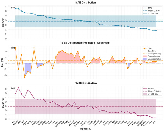
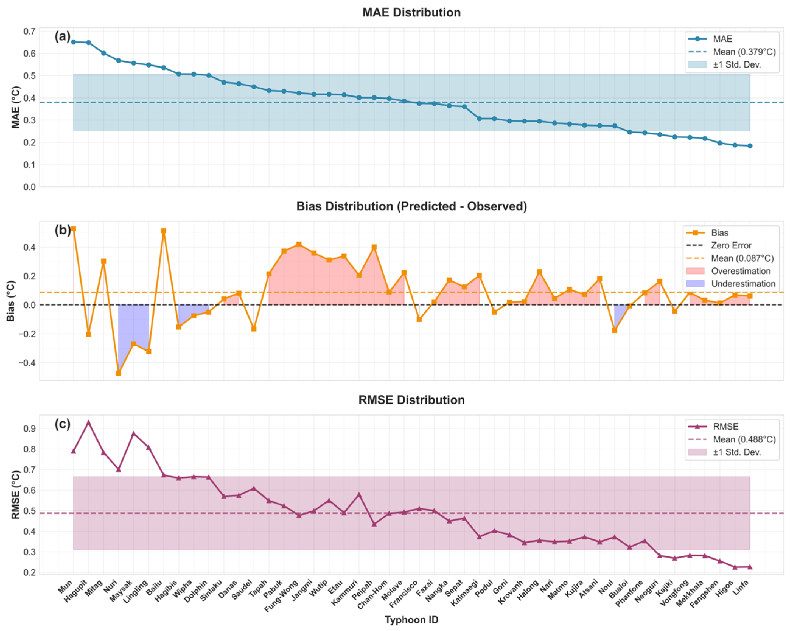
Figure 3a shows the MAE distribution across the 46 test typhoons. About 92% of the typhoons have an MAE below 0.6 °C, and 68% of the errors fall within one standard deviation (0.253–0.506 °C). This indicates that the model gives stable predictions. The Bias distribution (Figure 3b) shows a clear tendency for the model to overestimate the cooling. Among the 46 typhoons in the test set, 33 show a positive bias, and the average bias is 0.087 °C. For most typhoons, the prediction bias stays within 0.4 °C. For the 10 typhoons with the largest MAE, the average bias is −0.020 °C, with 7 negative and 3 positive biases. This means that most large errors come from underestimation, which is opposite to the overall overestimation trend. This suggests that when a typhoon causes very strong cooling, the model tends to underestimate it, leading to larger errors. The RMSE distribution is shown in Figure 3c. The spread of RMSE is much wider than that of MAE, indicating that while the model is generally accurate, a few large errors (up to 0.929 °C) have a strong impact on the RMSE.

Figure 3. Sequence distribution of SSC prediction errors: (a) MAE, (b) Bias, (c) RMSE. Typhoons are sorted in descending order based on their MAE values. The solid line represents the error value for each typhoon, the dashed line indicates the mean value, and the shaded area denotes the range of mean ± one standard deviation. In panel (b), the red and blue shadings represent the regions of overestimation and underestimation, respectively.

3.4. Spatial Distribution of SSC

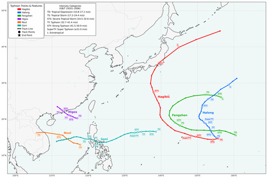
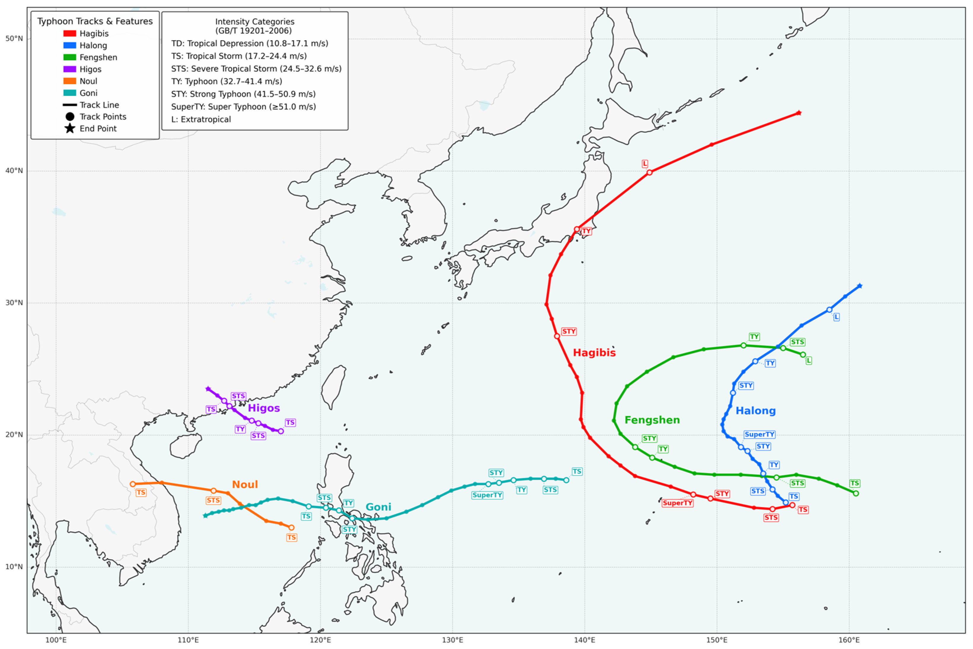
To test the applicability of this method in different typhoon cases, six typhoons in the Northwest Pacific from 2019 to 2020 are selected: Fengshen (2019), Noul (2020), Hagibis (2019), Higos (2020), Halong (2019), and Goni (2020), as shown in Figure 4. These typhoons cover a range of intensities, tracks, and ocean areas. Hagibis and Goni are strong and cover both open ocean and coastal areas. Noul and Higos are fast-growing and form quickly near the coast. Halong and Fengshen are autumn typhoons in the open ocean, with eastward tracks and long lifetimes.

Figure 4. Map of western Pacific typhoon tracks during 2019–2020, showing the best-track trajectories of six named typhoons (Hagibis, Halong, Fengshen, Higos, Noul, and Goni) at 6 h intervals. Each typhoon is represented by a distinct color, with track points marked by solid circles and endpoints indicated by stars. White circles connected by dashed lines mark key transition nodes in intensity classification, with labels indicating intensity categories [42].

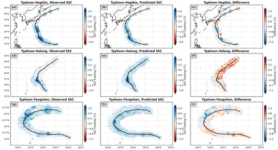
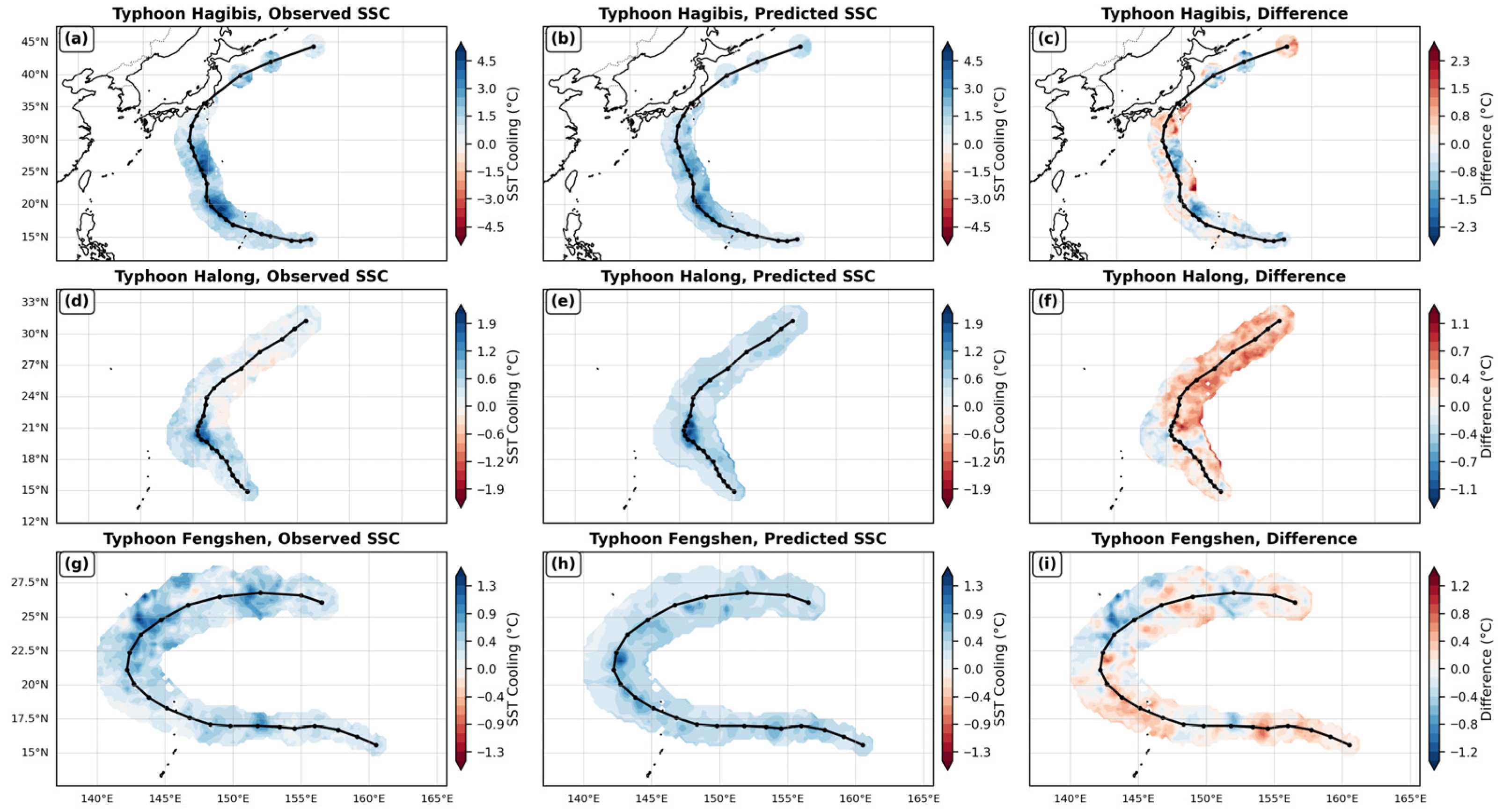
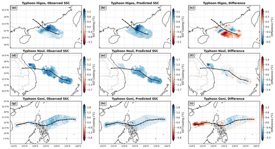
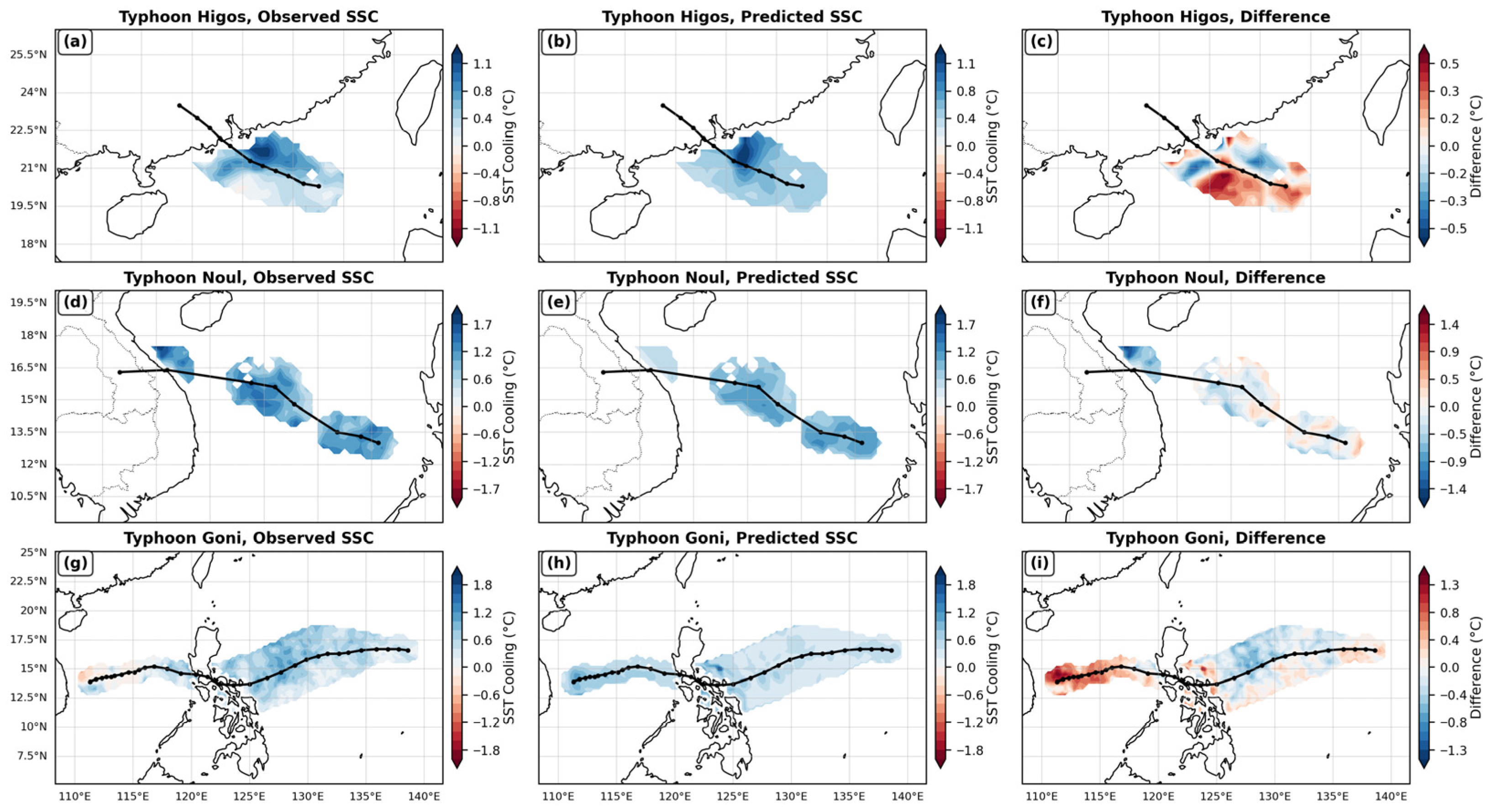
Figure 5 and Figure 6 compare the observed and predicted SSC spatial distributions for the six typhoons. In most cases, the SSC distribution was asymmetric, with the maximum cooling generally located on the right side of the typhoon track. This is because Ekman pumping and vertical mixing are stronger on the right side, consistent with previous studies [12,13]. For example, Typhoon Hagibis produced a crescent-shaped cold wake with a maximum cooling of 4.96 °C, located about 39.2 km to the right of the track. Typhoon Halong and Higos also showed rightward-biased cooling, with maximum cooling of 2.05 °C (4.1 km to the right) and 1.26 °C (64.3 km to the right), respectively. Typhoon Noul had a maximum cooling of 1.94 °C, located 124.5 km to the right. Typhoon Goni, moving slowly east of the Philippines, formed a northeast-southwest cooling zone on the right side of the track with a maximum cooling of 1.29 °C. These examples all show the common feature of rightward-biased cooling. However, Typhoon Fengshen was different: its maximum cooling center (1.47 °C) was about 950 km to the left of the track, indicating that background circulation or asymmetric typhoon structure can sometimes dominate the cooling distribution.

Figure 5. Comparison of observed, predicted, and differential SSC induced by typhoons in 2019: (a–c) Hagibis, (d–f) Halong, (g–i) Fengshen. The first column shows observed SSC, the second column shows model-predicted SSC, and the third column shows the difference between prediction and observation (predicted minus observed).

Figure 6. Comparison of observed, predicted, and differential SSC induced by typhoons in 2020: (a–c) Higos, (d–f) Noul, (g–i) Goni. The first column shows observed SSC, the second column shows neural network-predicted SSC, and the third column shows the difference between prediction and observation (predicted minus observed).

The model reproduced the overall SSC distribution and intensity reasonably well. Some predictions were very accurate. For Typhoon Higos, the predicted maximum cooling was 1.25 °C (at 21.75°N, 114.75°E), which matched the observed 1.26 °C well. For Typhoon Halong, the difference between the predicted and observed maximum cooling was only 0.006 °C. These results indicate that the model’s outputs are broadly consistent with observations, and it performs better in open ocean areas or regions with simple topography. However, the model still had limitations in predicting spatial details and in specific ocean environments. For Typhoon Halong, the predicted cooling center was offset about 114 km to the northeast of the observed center. For Typhoon Noul, the observed maximum cooling was located to the right-front of the track (17.5°N, 107.5°E), but the model placed it to the left and south (13.0°N, 115.75°E). When a typhoon is strong and moves slowly, the wind stress acts longer and the cold wake becomes larger. The model did not fully capture this relationship between typhoon speed and ocean response.

In terms of cooling intensity, model errors were often related to specific regions or typhoon stages. For Typhoon Goni, the predicted maximum cooling (1.99 °C) was higher than the observed value (1.29 °C), and the predicted cooling area was more concentrated and stronger. This may be because the model overestimated the wind stress near the typhoon center or the vertical mixing efficiency. For Typhoons Noul and Fengshen, the model underestimated the maximum cooling, with errors of −1.54 °C and −1.29 °C, respectively. This may be due to poor representation of local stratification conditions. After Typhoon Goni hit the Philippines and re-entered the sea, the model did not fully account for the intensity reduction over land and overestimated the cooling, with a local error of +1.40 °C.

Looking at the spatial distribution of errors, the model performed poorly in regions where typhoon intensity or speed changed rapidly, or where ocean topography and stratification strongly interacted. In coastal areas (e.g., near Japan during Typhoon Hagibis), the model often overestimated cooling. This may be related to uncertainties in shallow water effects and boundary layer friction parameterization. In the northern slope of the South China Sea (e.g., the area affected by Typhoon Noul), model errors increased significantly, indicating that the model has not yet fully captured how complex terrain modulates upper ocean dynamics.

3.5. Cooling Structure Along and Across the Typhoon Track

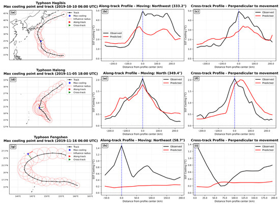
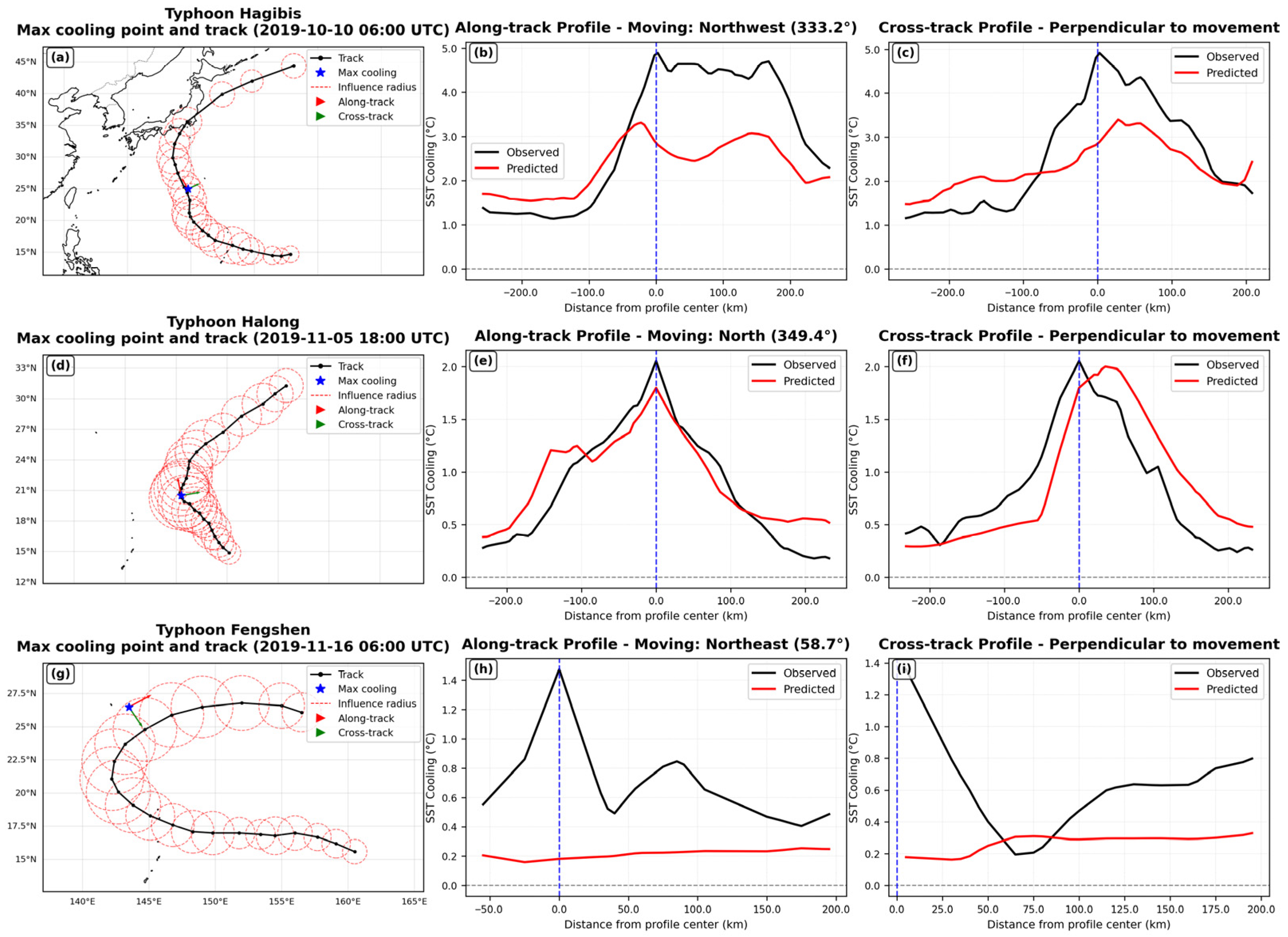
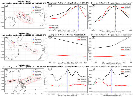
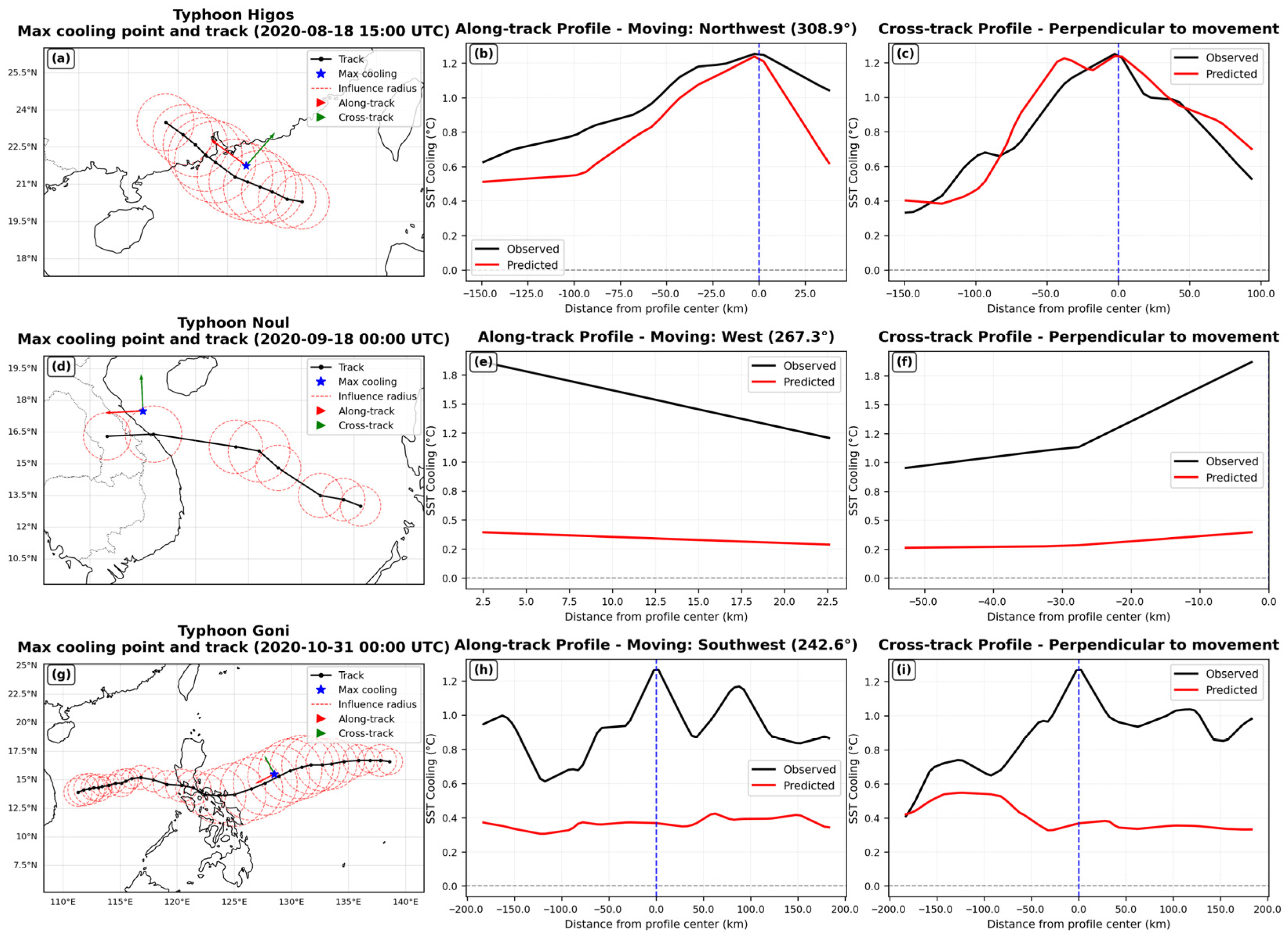
To study the spatial pattern of SSC during typhoons and to test how well the model captures key dynamic processes, we took the observed maximum cooling point of each typhoon as the analysis center. This point is defined as the grid cell with the highest observed SSC within the 8-wind circle. From this center, we extracted two profiles: one along the typhoon track (along-track), which reflects the cumulative cooling effect and wake development, and one perpendicular to the track (cross-track). In the cross-track profile, positive values represent the right side of the track and negative values the left side, which helps to show the asymmetry caused by the Coriolis force and wind field structure. Based on these definitions, we plotted the observed and predicted SSC profiles (Figure 7 and Figure 8).

Figure 7. Cooling analysis at the maximum SSC point during Typhoons Hagibis, Halong, and Fengshen in 2019: Along-track and cross-track profiles. (a,d,g) Typhoon track maps showing the typhoon movement path and profile center locations; (b,e,h) SSC profiles along the typhoon movement direction; (c,f,i) SSC profiles perpendicular to the typhoon movement direction. Blue dotted lines indicate the location of the profile center.

Figure 8. Cooling analysis at the maximum SSC point during Typhoons Higos, Noul, and Goni in 2020: Along-track and cross-track profiles. (a,d,g) Typhoon track maps showing the typhoon movement path and profile center locations; (b,e,h) SSC profiles along the typhoon movement direction; (c,f,i) SSC profiles perpendicular to the typhoon movement direction. Blue dotted lines indicate the location of the profile center.

The along-track profiles show a dynamic asymmetry caused by typhoon movement. For typhoons Hagibis, Fengshen, Higos and Goni, the observed cooling was much stronger behind the typhoon than ahead. This is because the wind behind a moving typhoon acts on the ocean for a longer time, leading to a larger accumulated effect from Ekman pumping, and the upwelled cold water experiences more sustained mixing. The model generally underestimated the cooling magnitude along the track. For example, for Hagibis and Higos, the predicted profile shapes were similar to the observed ones, but the cooling values were too low. For Halong, the observed cooling was nearly symmetric around the maximum cooling point; the model reproduced this pattern but underestimated the cooling within about ±100 km of the center (maximum underestimate −0.225 °C) and overestimated it farther away. This suggests that the model does not respond strongly enough to the strongest wind stress near the center. For Fengshen and Noul, the predicted SSC profiles were almost flat in both along-track and cross-track directions, failing to capture the actual spatial variations, and the predicted values were generally too low. This may be because their maximum cooling points were located near the edge of the 8-wind circle, and the model inputs rely too much on wind speeds near the typhoon center, missing the ocean response at the edges.

In the Northern Hemisphere, the Coriolis force and cyclonic circulation make the strongest wind stress, ocean mixing and upwelling occur on the right side of the track. This pushes the maximum cooling center to the right. The cross-track profiles confirm this: except for Fengshen, the maximum SSC of the other typhoons was on the right side, consistent with the previous section. For Hagibis, the model underestimated the cooling on the right side (positive cross-track direction) and overestimated it about 100 km to the left (negative direction). For a simple, less intense typhoon like Higos, the model performed well in the cross-track direction, with an average bias of only 0.042 °C, better than in the along-track direction. This shows that the model can simulate the lateral mixing processes driven by the Coriolis force and basic wind field for such typhoons. For Halong, the observed cross-track SSC profile was nearly symmetric, but the predicted cooling center was shifted to the right by 35.3 km, with overestimation on the right side and underestimation on the left. This may be because the input wind field had an unrealistic right-side enhancement, or because the mixing parameterization is too sensitive to lateral changes. For Noul and Goni, the model consistently underestimated the cross-track SSC, with predicted mean values of 0.308 °C and 0.547 °C, respectively, compared to observed values of 1.285 °C and 1.268 °C. This suggests that in areas affected by complex topography, the model may underestimate lateral energy input and mixing efficiency.

3.6. Analysis of Prediction Error Sources

To better understand the vertical physical processes of typhoon-induced SSC and how they affect prediction errors, we selected analysis points for six typical typhoons. These points are located on both sides of the typhoon tracks and cover different marine environments, including deep open ocean, continental slopes, and shallow shelves. By analyzing the evolution of upper-ocean temperature profiles at these points, together with ocean parameters such as MLD and thermocline gradient (defined as the average temperature gradient from the bottom of the mixed layer to 100 m below), we examined the causes and patterns of prediction errors related to vertical structure.

3.6.1. Influence of Initial Ocean Stratification

Typhoon-induced SSC and its prediction accuracy depend not only on typhoon intensity but also on the initial thermal structure of the upper ocean. MLD and thermocline gradient are two key background parameters. A shallow MLD means the upper ocean has low heat capacity and is more sensitive to wind stress, which can easily lead to surface cooling. A strong thermocline acts as a barrier to vertical mixing and prevents cold water from rising.

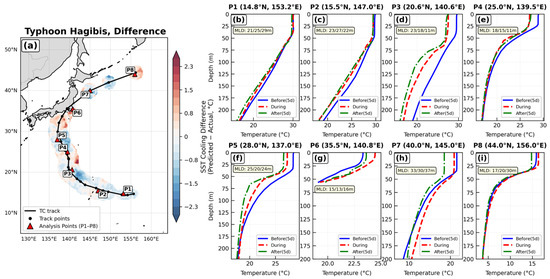
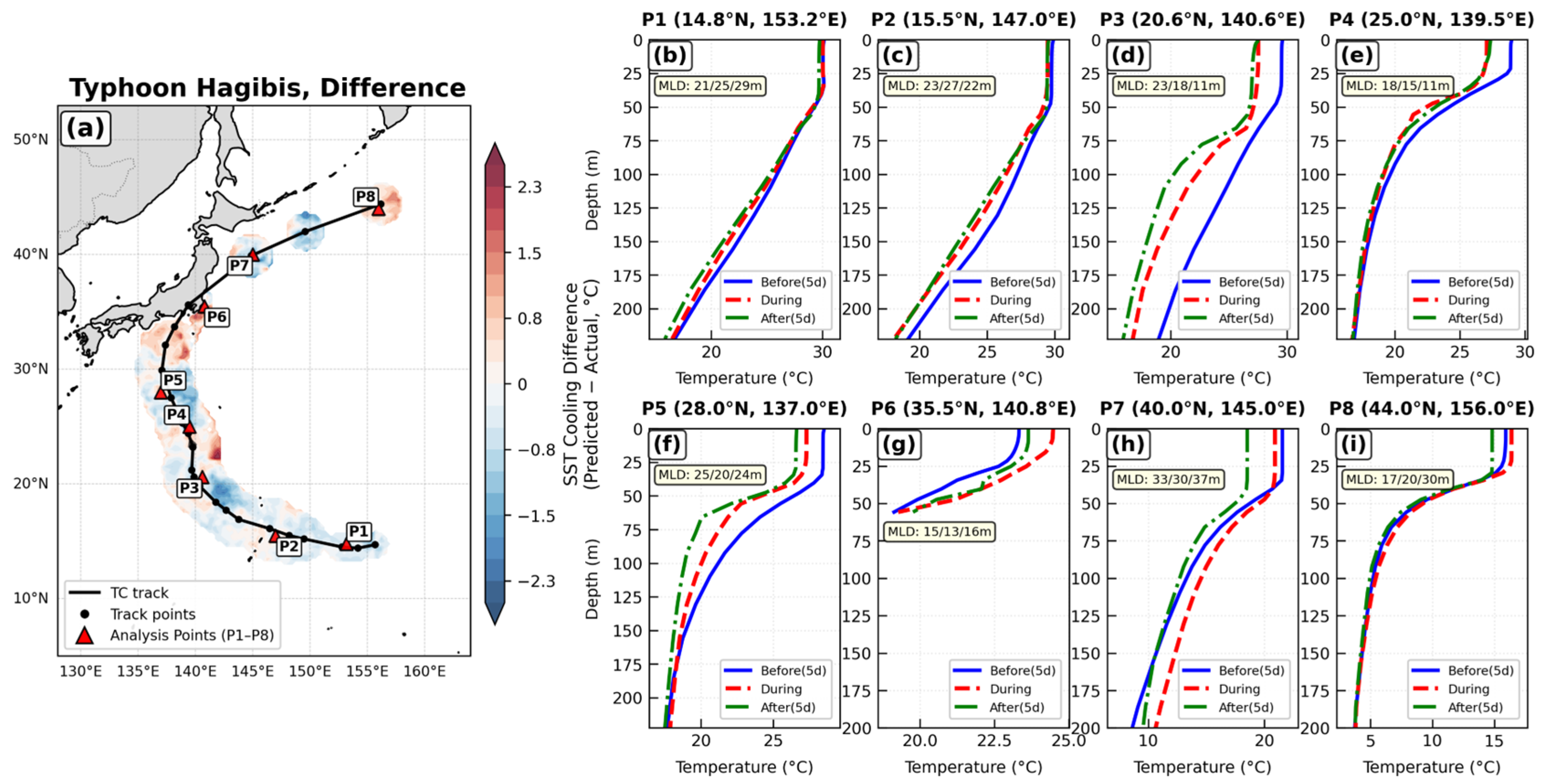
Typhoon Hagibis (2019) moved from low to mid-high latitudes and passed through different ocean environments (Figure 9, Table 4). In open deep-water areas with uniform stratification and moderate thermocline gradient (points P2 and P3), MLD was about 23 m and thermocline gradient was 0.056–0.061 °C/m. Prediction errors were less than 0.1 °C, showing that the model can simulate vertical mixing well under moderate conditions. In more complex ocean conditions, errors became larger. At point P4, MLD was only 18 m, and the thermocline gradient was 0.052 °C/m. The upper ocean had low heat capacity and weak vertical stability. The typhoon caused strong entrainment, and the observed cooling reached 4.96 °C, but the model underestimated it by 2.12 °C. This indicates that the model struggles to simulate strong entrainment and upwelling. Differences in thermocline gradient also affected model errors. Points P5 and P8 had similar MLD values but different thermocline gradients. At P5, the gradient was weak (0.063 °C/m), and the model overestimated cooling by 1.16 °C. At P8, the gradient was strong (0.139 °C/m), and the prediction was more accurate. This shows that a strong thermocline suppresses vertical mixing and makes the ocean response more stable and easier to predict. The model also had limitations in areas with deep mixed layers. Point P7 was in open water outside Tokyo Bay. Its MLD was 33 m, the deepest among all selected points. The initial heat capacity was large, and the observed cooling was weak. The model underestimated cooling by 1.11 °C, possibly because it underestimated vertical mixing efficiency in deep mixed layers.

Figure 9. Difference between observed and model-predicted SSC for Typhoon Hagibis (2019) (a), and upper ocean temperature profiles (b–i) at locations indicated by the red triangles in (a). Solid, dashed, and dotted lines represent vertical temperature profiles before, during, and after the typhoon, respectively.

Table 4. Initial ocean state parameters and SSC prediction errors at selected points during the passage of Typhoon Hagibis.

Point	Latitude	Longitude	Observed Cooling (°C)	Predicted Cooling (°C)	Prediction Error (°C)	MLD (m)	Thermocline Gradient (°C/m)
P1	14.8	153.2	1.19	0.74	−0.45	21	0.0711
P2	15.5	147.0	1.14	1.07	−0.07	23	0.0569
P3	20.6	140.6	4.22	4.23	+0.01	23	0.0607
P4	25.0	139.5	4.96	2.84	−2.12	18	0.0521
P5	28.0	137.0	1.19	2.35	+1.16	25	0.0626
P6	35.5	140.8	1.02	1.22	+0.20	15	0.1132
P7	40.0	145.0	1.75	0.65	−1.11	33	0.0899
P8	44.0	156.0	1.09	1.05	−0.04	17	0.1394

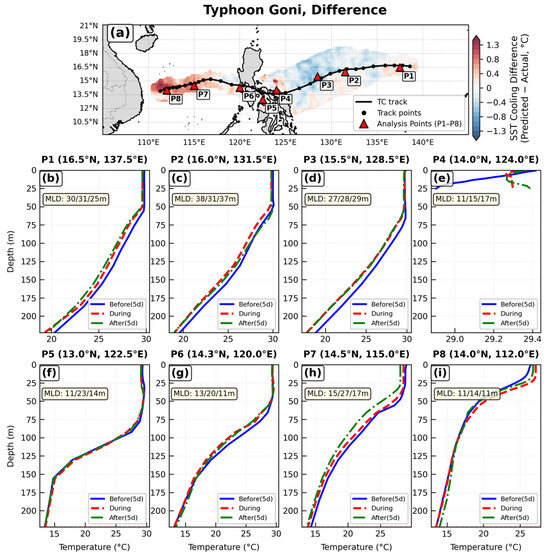
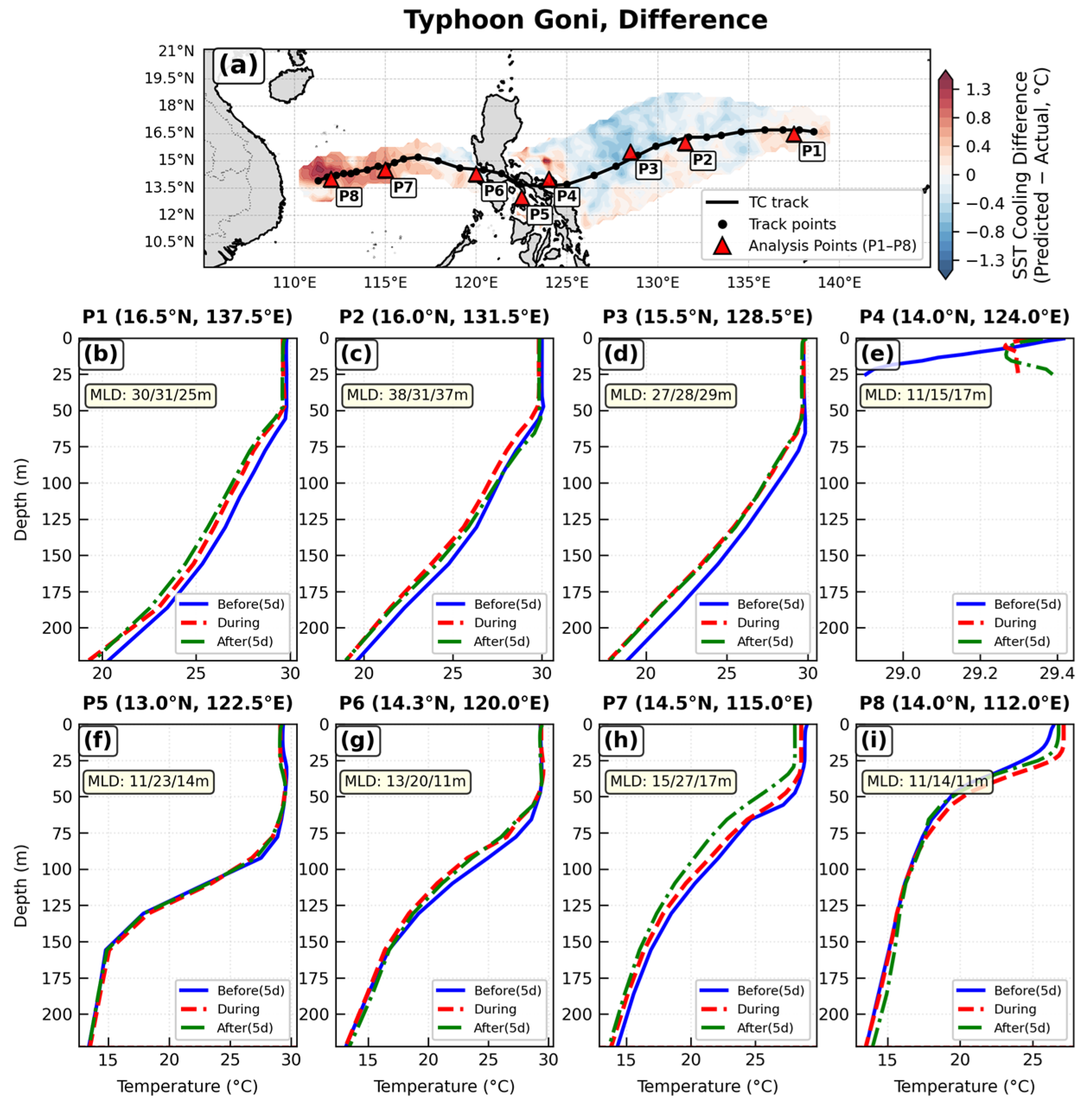
In the case of Typhoon Goni in 2020 (Figure 10, Table 5), a similar pattern was observed. For example, at point P2, the initial MLD was 38 m, indicating a large heat capacity. The thermocline gradient was 0.0554 °C/m, which did not strongly inhibit vertical mixing. Under these conditions, the ocean response to typhoon forcing was mainly driven by wind stress. The model predicted a cooling of 0.50 °C, which was close to the observed cooling of 0.54 °C.

Figure 10. Difference between observed and model-predicted SSC for Typhoon Goni (2020) (a), and upper ocean temperature profiles (b–i) at locations indicated by the red triangles in (a). Solid, dashed, and dotted lines represent vertical temperature profiles before, during, and after the typhoon, respectively.

Table 5. Initial ocean state parameters and SSC prediction errors at selected points during the passage of Typhoon Goni.

Point	Latitude	Longitude	Observed Cooling (°C)	Predicted Cooling (°C)	Prediction Error (°C)	MLD (m)	Thermocline Gradient (°C/m)
P1	16.5	137.5	0.31	0.48	0.17	30	0.0470
P2	16	131.5	0.54	0.50	−0.04	38	0.0554
P3	15.5	128.5	1.29	0.37	−0.92	27	0.0524
P4	14	124	0.46	0.46	0	11	nan
P5	13	122.5	0.60	0.99	0.39	11	0.1121
P6	14.3	120	0.80	0.51	−0.3	13	0.1098
P7	14.5	115	−0.14	0.67	0.82	15	0.1055
P8	14	112	0.03	0.67	0.64	11	0.0408

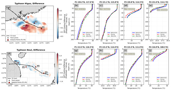
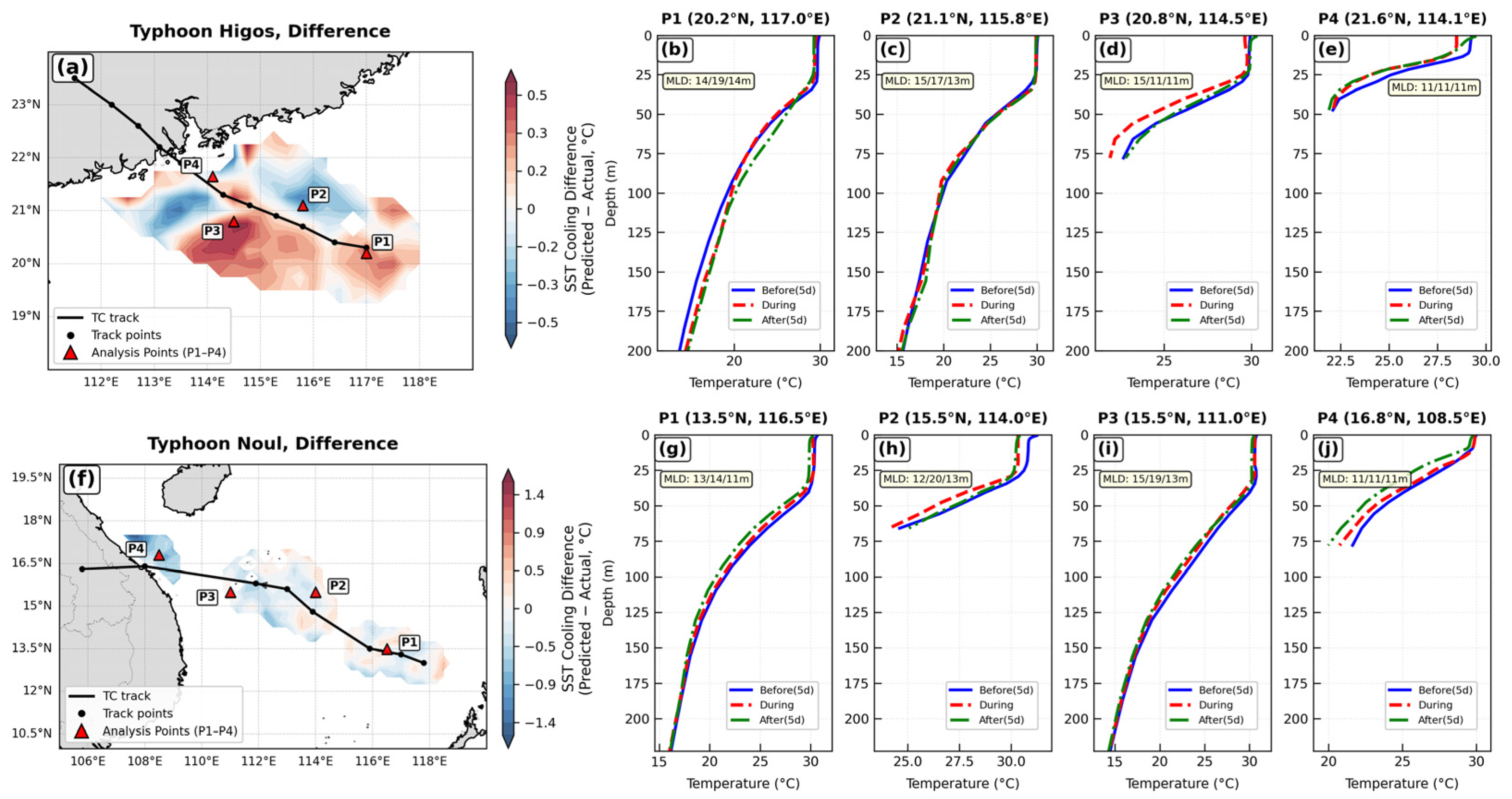
The effect of thermocline gradient can also be seen in Typhoon Higos (Figure 11a–e, Table 6). At point P4, the thermocline gradient was the strongest (0.2214 °C/m). The strong stratification suppressed vertical mixing, making the cooling mechanism simple. The model error was small (−0.08 °C), and prediction accuracy was high. Typhoon Noul (Figure 11f–j, Table 7) also supports the above conclusions. Under similar initial MLD conditions (13 m at P1 and 15 m at P3), the deep open-water point P1 had a weak thermocline gradient (0.0865 °C/m). The model prediction was stable with an error of only +0.02 °C. At P3, where the thermocline gradient increased to 0.0934 °C/m, the error changed to −0.18 °C, suggesting that the model may overreact to the mixing suppression effect.

Figure 11. Difference between observed and model-predicted SSC for Typhoon Higos (2020) (a), and upper ocean temperature profiles (b–e) at locations indicated by the red triangles in (a); and difference between observed and model-predicted SSC for Typhoon Noul (2020) (f), and upper ocean temperature profiles (g–j) at locations indicated by the red triangles in (f). Solid, dashed, and dotted lines represent vertical temperature profiles before, during, and after the typhoon, respectively.

Table 6. Initial ocean state parameters and SSC prediction errors at selected points during the passage of Typhoon Higos.

Point	Latitude	Longitude	Observed Cooling (°C)	Predicted Cooling (°C)	Prediction Error (°C)	MLD (m)	Thermocline Gradient (°C/m)
P1	20.2	117.0	0.07	0.45	+0.37	14	0.0926
P2	21.1	115.8	0.70	0.52	−0.18	15	0.0926
P3	20.8	114.5	0.21	0.72	+0.51	15	0.0846
P4	21.6	114.1	0.81	0.74	−0.08	11	0.2214

Table 7. Initial ocean state parameters and SSC prediction errors at selected points during the passage of Typhoon Noul.

Point	Latitude	Longitude	Observed Cooling (°C)	Predicted Cooling (°C)	Prediction Error (°C)	MLD (m)	Thermocline Gradient (°C/m)
P1	13.5	116.5	0.96	0.98	+0.02	13	0.0865
P2	15.5	114.0	0.80	0.62	−0.18	12	nan
P3	15.5	111.0	0.78	0.60	−0.18	15	0.0934
P4	16.8	108.5	1.22	0.54	−0.68	11	0.0663

3.6.2. Influence of Complex Terrain

In shallow coastal areas with complex terrain, the ocean response to typhoons differs from that in the open ocean. Prediction errors here depend not only on typhoon dynamics and ocean stratification, but also on water depth, bottom friction, and lateral energy redistribution. These factors make the model less reliable in shallow waters.

Take Typhoon Higos (2020) as an example (Figure 11a–e, Table 6). The largest error occurred at P3, a shallow-water point. The typhoon was at its peak intensity. The initial MLD was 15 m, and the thermocline gradient was weak (0.0846 °C/m). These conditions should favor vertical mixing. However, the model overestimated cooling by 0.51 °C. In shallow water, strong wind stress can be quickly dissipated by bottom friction, and some energy is redistributed by horizontal advection, which reduces vertical mixing efficiency. The mixing parameterization, originally developed for open oceans, does not capture the suppression effect of shallow terrain.

A similar pattern is seen in Typhoon Noul (Figure 11f–j, Table 7). The shallow-water points P2 and P4 (water depth < 100 m) showed much larger errors than the deep-water point P1. P2 had an MLD of only 12 m, and the model underestimated cooling by 0.18 °C. At P4, MLD was 11 m and the thermocline gradient was 0.0663 °C/m. The model underestimated cooling by 0.68 °C, and the observed cooling (1.22 °C) was more than twice the prediction (0.54 °C). In shallow water, a shallow mixed layer and a weak thermocline gradient both promote vertical mixing. Typhoon forcing can easily trigger strong bottom friction mixing and vertical entrainment. However, the current model lacks adequate parameterization for shallow-water mixing and bottom boundary layer processes, which leads to underestimation of cooling.

Typhoon Goni also shows the effect of complex terrain (Figure 10, Table 5). At P4, east of Luzon Island, the water is shallow. The model prediction agreed well with observations, suggesting that in a shallow mixed layer without strong stratification, wind-driven mixing can be simulated reasonably well. At P5, which is located in a narrow channel between Philippine islands, the stratification was strong. The model overestimated cooling by 0.39 °C. Observations showed that the mixed layer deepened sharply from 11 m to 23 m during the typhoon and then quickly returned to 14 m after its passage. The temperature profile was stepped. Strong stratification suppressed vertical entrainment, and the observed cooling was mainly due to horizontal advection and terrain-induced mixing. However, the model overestimated the role of vertical entrainment. At P7, in the deep basin of the South China Sea, the observed sea surface temperature actually increased slightly, but the model still predicted notable cooling, with an error of 0.82 °C. This suggests that in this region, temperature changes during the typhoon may be dominated by advection rather than vertical mixing. The model failed to distinguish between these two mechanisms. At P8, on the continental slope, the observed cooling was very weak. However, the model still predicted significant cooling under weak stratification. This may be because the typhoon had weakened by the time it reached this area, and vertical mixing efficiency had decreased. But the model did not capture this reduction in forcing and continued to use mixing parameters suitable for strong winds, leading to overestimation.

3.6.3. Influence of Typhoon Dynamic Structure

Prediction errors are not only affected by ocean conditions, but also by how the typhoon itself evolves. Changes in typhoon intensity, speed, or track can alter how the typhoon forces the ocean. The current model cannot fully capture these changes, which is a key source of error.

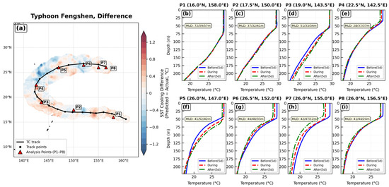
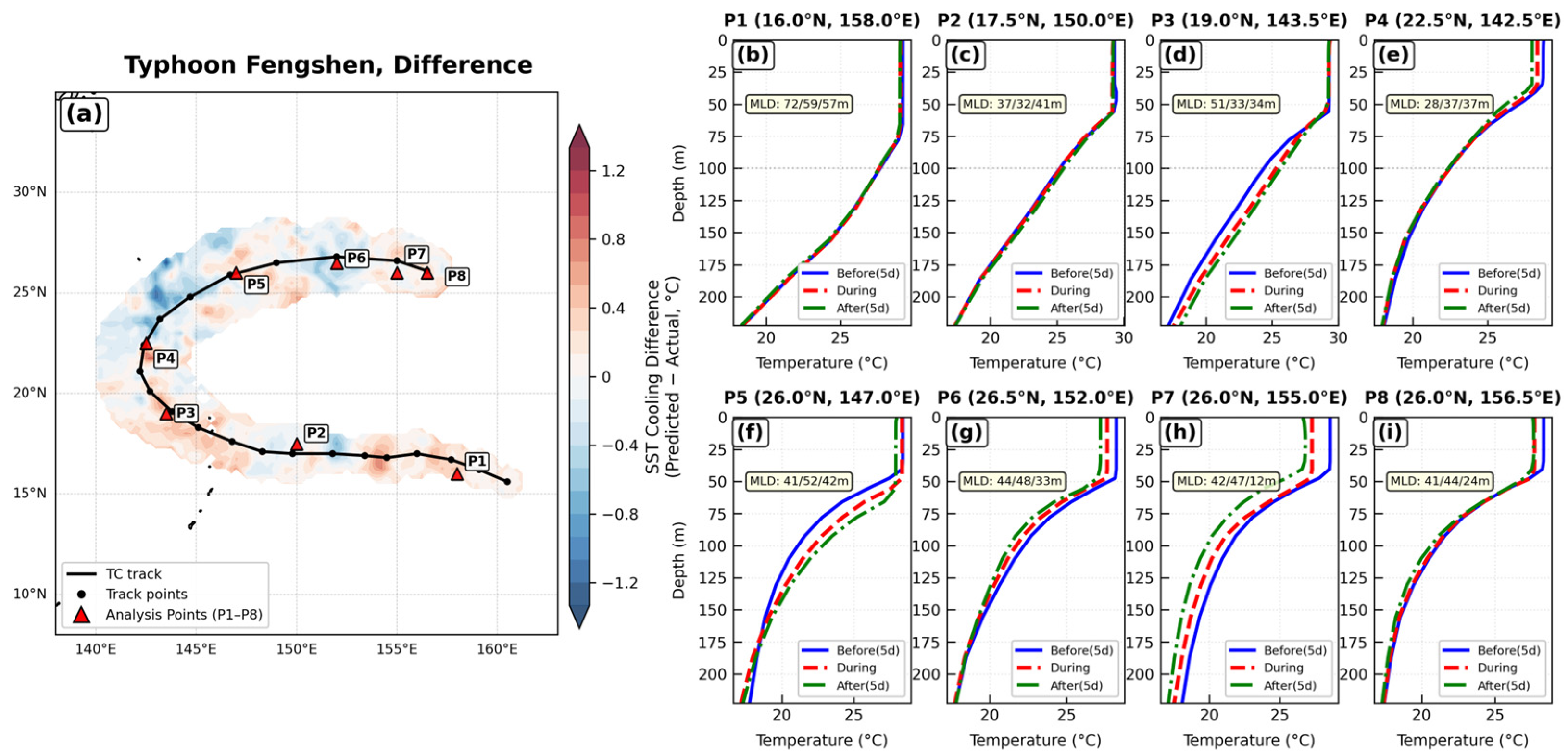
Taking Typhoon Fengshen as an example (Figure 12, Table 8). Its complex turning path helps us understand how typhoon dynamics and ocean stratification interact. The model often overestimated cooling, especially during the early stage, the turning point, and the dissipation stage. This shows that the model has difficulty simulating ocean responses when both the track and intensity change rapidly. Near the turning point P3, the background thermocline gradient was strong (0.0893 °C/m), and the mixed layer depth shallowed from 51 m to 34 m. This means the strong stratification reduced vertical mixing. Still, the model overestimated cooling by 0.21 °C. This may be because the changing wind field altered the interaction between wind stress and the background ocean flow. The model was developed for typhoons moving steadily, so it struggles with sudden changes. Overestimation also appeared at other stages. At P1 (early stage), the mixed layer was deepest (72 m) and the thermocline gradient was weakest (0.0501 °C/m). This suggests a large heat capacity. In theory, a deep mixed layer allows energy to be mixed downward. But the actual typhoon was weak at this stage, and the wind stress was not strong enough to stir the deep water. The observed cooling was only 0.27 °C. The model overestimated it (error +0.18 °C), suggesting it overestimates mixing efficiency for weak typhoons in deep mixed layers. After the typhoon turned and began to weaken (P4, P5, P7, P8), the typhoon intensity decreased, movement became more stable, and ocean stratification was moderate to strong (thermocline gradient 0.0676–0.0755 °C/m). Still, the model continued to predict strong cooling. This means it failed to account for the reduced wind stress and mixing efficiency during the weakening stage, and did not adapt well to the new balance between wind field and ocean response after the turn. In contrast, during the westward intensifying stage (P2) and the post-turn weakening stage (P6), the typhoon moved steadily and intensity changed smoothly. Model errors were small, with slight underestimation (−0.07 °C and −0.13 °C). This shows that when the typhoon dynamics are stable and ocean response is gradual, the model performs reliably.

Figure 12. Difference between observed and model-predicted SSC for Typhoon Fengshen (2019) (a), and upper ocean temperature profiles (b–i) at locations indicated by the red triangles in (a). Solid, dashed, and dotted lines represent vertical temperature profiles before, during, and after the typhoon, respectively.

Table 8. Initial ocean state parameters and SSC prediction errors at selected points during the passage of Typhoon Fengshen.

Point	Latitude	Longitude	Observed Cooling (°C)	Predicted Cooling (°C)	Prediction Error (°C)	MLD (m)	Thermocline Gradient (°C/m)
P1	16.0	158.0	0.27	0.45	+0.18	72	0.0501
P2	17.5	150.0	0.37	0.29	−0.07	37	0.0813
P3	19.0	143.5	0.33	0.53	+0.21	51	0.0893
P4	22.5	142.5	0.70	0.80	+0.10	28	0.0676
P5	26.0	147.0	0.20	0.28	+0.08	41	0.0755
P6	26.5	152.0	0.54	0.41	−0.13	44	0.0768
P7	26.0	155.0	0.16	0.23	+0.08	42	0.0742
P8	26.0	156.5	0.30	0.49	+0.19	41	0.0755

In Typhoon Goni (Figure 10, Table 5), at the peak intensity stage (P3), the initial mixed layer was 27 m and the thermocline gradient was moderate (0.0524 °C/m). The stratification was not extreme. However, the strong and sustained wind stress caused a strong dynamic response. The observed cooling was 1.29 °C, but the model predicted only 0.37 °C (error −0.92 °C). During the typhoon, the mixed layer deepened by only about 1 m. This suggests that the cooling was mainly driven by upwelling and near-inertial pumping, which are nonlinear processes. The current model does not capture these mechanisms well.

Typhoon Higos (Figure 11a–e, Table 6) also shows how typhoon development stage affects prediction errors. At deep-water points P1 and P2, the thermocline gradient (0.0926 °C/m) and mixed layer depth (14–15 m) were similar, but prediction errors differed. At P1, which was in the early stage of the typhoon, wind stress was weak, and the model overestimated cooling by 0.37 °C. At P2, which was in the rapid intensification stage, the model performed better (underestimated by 0.18 °C). This indicates that the model is more reliable when intensity increases steadily, but tends to overestimate cooling during weak forcing in the early stage.

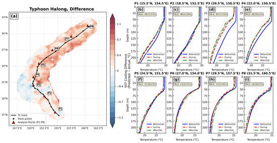
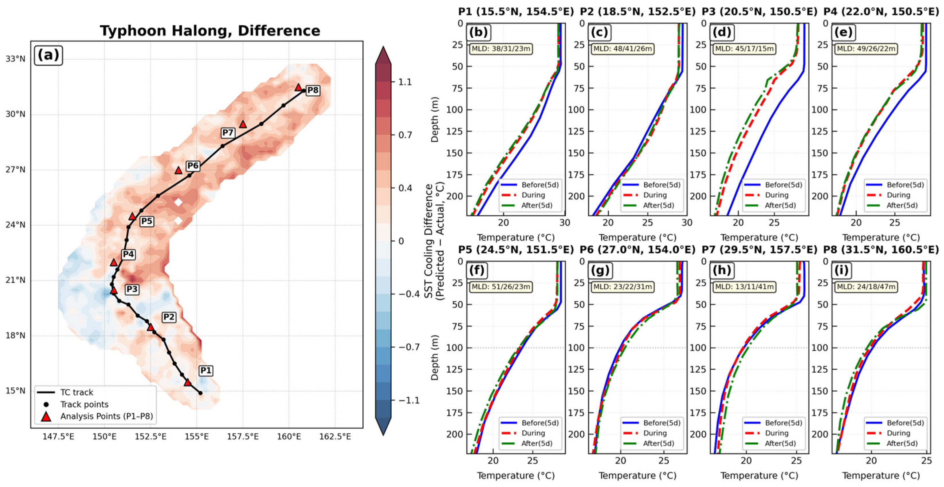
In the case of Typhoon Halong (Figure 13, Table 9), the model performed well during the rapid intensification and peak intensity stages (points P2 and P3). The prediction errors were −0.05 °C and −0.25 °C, both indicating slight underestimation. This suggests that under strong wind forcing, the model captures the mixing processes reasonably well. However, during the early formation, weakening stage, and outer regions (points P1 and P4–P8), the model generally overestimated the cooling. The error increased with latitude and as the typhoon weakened. The most significant overestimation occurred at point P7. At this location, the initial mixed layer depth was only 13 m, and the thermocline gradient was weak. The model predicted a cooling of 0.48 °C, but the observed cooling was only 0.05 °C, resulting in an error of +0.43 °C. Although a shallow mixed layer theoretically makes the ocean more sensitive to forcing, the model still overestimated cooling under weak wind conditions. This may be because the model does not properly represent the rapid decay of mixing under weak forcing, nor does it fully account for the reduced forcing effect as the typhoon weakens and its wind energy becomes more dispersed.

Figure 13. Difference between observed and model-predicted SSC for Typhoon Halong (2019) (a), and upper ocean temperature profiles (b–i) at locations indicated by the red triangles in (a). Solid, dashed, and dotted lines represent vertical temperature profiles before, during, and after the typhoon, respectively.

Table 9. Initial ocean state parameters and SST cooling prediction errors at selected points during the passage of Typhoon Halong.

Point	Latitude	Longitude	Observed Cooling (°C)	Predicted Cooling (°C)	Prediction Error (°C)	MLD (m)	Thermocline Gradient (°C/m)
P1	15.5	154.5	0.25	0.40	+0.15	38	0.0727
P2	18.5	152.5	0.65	0.60	−0.05	48	0.0659
P3	20.5	150.5	2.05	1.80	−0.25	45	0.0727
P4	22.0	150.5	0.47	0.66	+0.19	49	0.0799
P5	24.5	151.5	0.17	0.45	+0.28	51	0.0805
P6	27.0	154.0	0.13	0.38	+0.25	23	0.0700
P7	29.5	157.5	0.05	0.48	+0.43	13	0.0661
P8	31.5	160.5	0.08	0.44	+0.36	24	0.0600

3.7. Analysis of Key Thermal and Dynamic Factors

3.7.1. Influence of Upper Ocean Thermal Structure

The cooling of sea surface temperature during a typhoon is largely controlled by the upper ocean thermal structure before the typhoon arrives. The commonly used Ocean Heat Content (OHC) index has clear limitations in shallow water, low temperature areas, or regions with strong salinity stratification. To better capture the mechanism of typhoon-induced cooling, Price [39] proposed the vertically averaged temperature $T_{\overline{100}}$ as a more reliable thermal index. It represents the average temperature from the sea surface down to 100 m depth and can effectively predict sea surface temperature changes after a typhoon. Following Price’s theory, Guan et al. [43] applied $T_{\overline{100}}$ to shallow seas such as the Yellow Sea and the Bohai Sea. They further developed a temperature anomaly parameter: $T_a=SST-T_{\overline{100}}$. A larger $T_a$ means a stronger vertical temperature gradient in the upper ocean, which indicates greater potential for sea surface cooling under typhoon forcing. A smaller $T_a$ means weaker cooling potential. $T_a$ serves as a combined indicator of mixed layer depth, thermocline strength, and other factors. It directly reflects the cooling potential stored in the upper ocean.

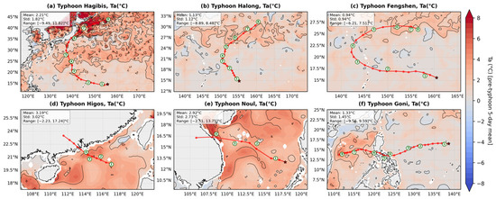
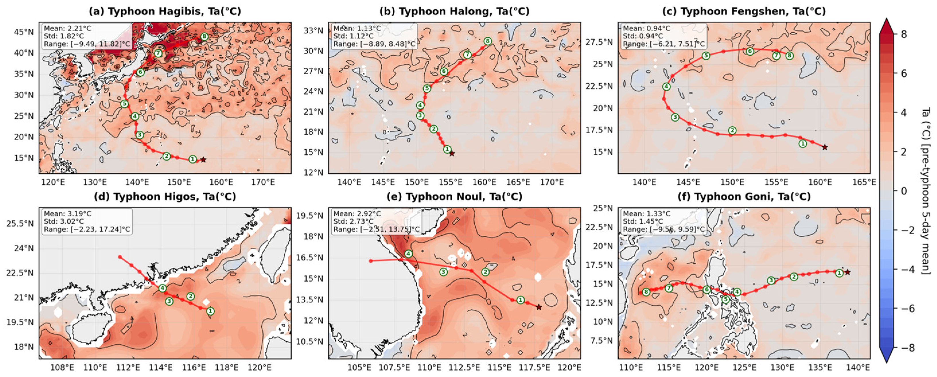
For each selected typhoon, the average $T_a$ value for the five days before the typhoon arrival was calculated. The results are shown in Figure 14. For most typhoons, $T_a$ tends to increase along their tracks. For example, along the path of Typhoon Hagibis, $T_a$ rose by about 6.99 °C, meaning it gradually moved into areas with a deeper thermocline and stronger stratification. The average $T_a$ along the tracks of Typhoons Higos and Noul exceeded 3 °C, indicating that the waters they passed through had the thermal conditions for strong negative ocean feedback. After Typhoon Goni entered the South China Sea, its $T_a$ quickly increased from negative values east of the Philippines to 4.46 °C, reflecting a significant increase in stratification.

Figure 14. Spatial distribution of the pre-typhoon 5-day average temperature anomaly ($T_a$) for each typhoon. Selected points are marked by white circles with green numbers. (a) Hagibis; (b) Halong; (c) Fengshen; (d) Higos; (e) Noul; (f) Goni.

A further comparison between $T_a$ and prediction error shows that at points with high initial $T_a$, the model generally underestimates the cooling. For example, at points P4 and P7 of Typhoon Hagibis, $T_a$ was 4.24 °C and 4.28 °C, and the prediction errors were −2.12 °C and −1.11 °C. This means the actual cooling was stronger than the model predicted in strongly stratified areas. In contrast, at points with low initial $T_a$, such as most points along the path of Typhoon Fengshen ($T_a<1 °\mathrm{C}$) and the early part of Typhoon Goni’s path ($T_a<0.5 °\mathrm{C}$), the prediction errors were generally small. This indicates that the cooling effect is weaker in weakly stratified areas, and the model performs more stably there.

Under strong typhoon forcing, a strong vertical temperature gradient in high $T_a$ areas promotes turbulent mixing and upwelling of cold water, leading to significant cooling. However, existing models often rely on sea surface temperature or mixed layer heat content at a fixed depth. They cannot fully capture the full-layer thermal gradient information represented by $T_a$. Therefore, when typhoons enter significantly stratified areas such as the northern South China Sea, the Yellow Sea, or the Kuroshio Extension, the model often underestimates the cooling.

3.7.2. Role of Mesoscale Eddies

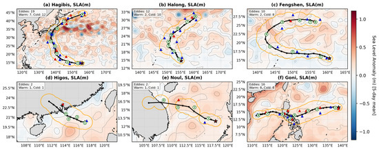
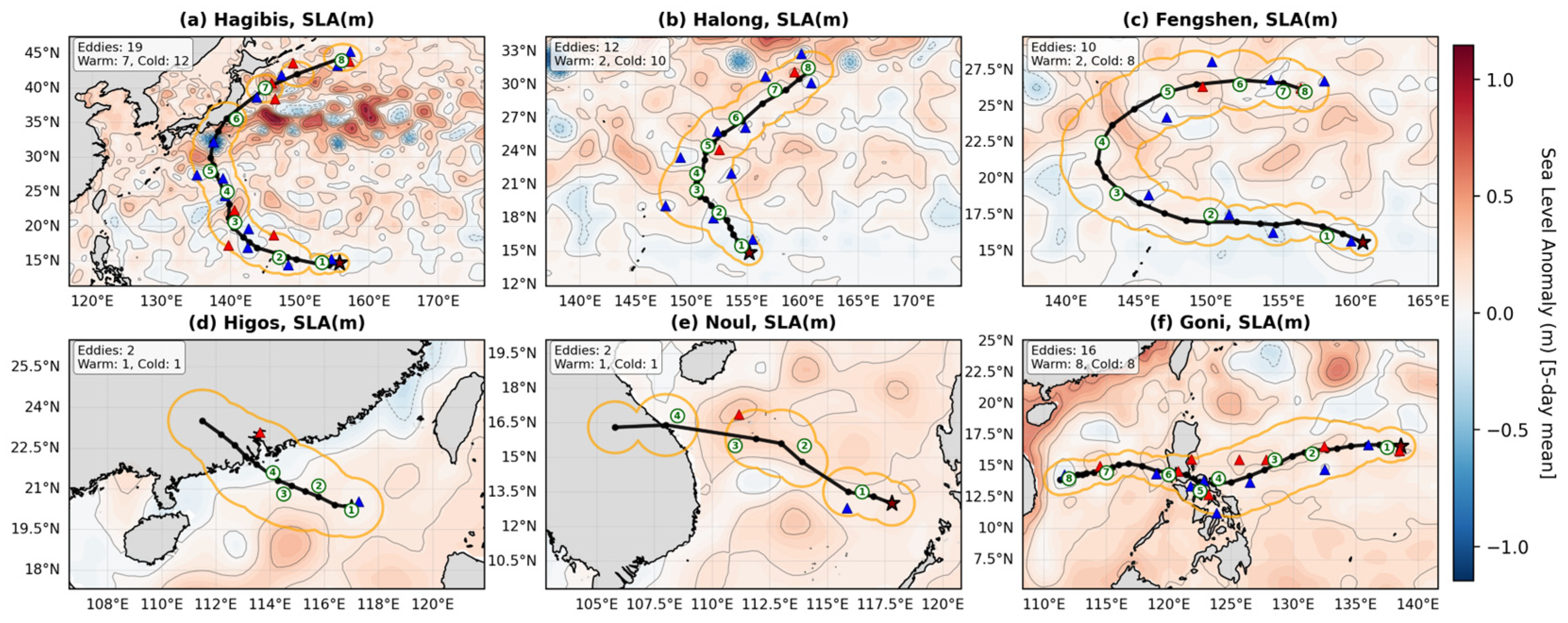
Background ocean processes such as eddies can change sea surface height. When a tropical cyclone passes over a cold eddy (CE), the cooling is usually stronger. When it passes over a warm eddy (AE), the cooling tends to be weaker [44,45,46,47,48]. In cold eddy areas, strong upwelling brings deep cold water to the surface, creating a “cold suction” effect. This causes large cooling that can reach down to 700 m or more. In warm eddy areas, cooling mainly comes from vertical mixing, which is generally weaker [45,46]. These different mechanisms explain how different eddies affect sea surface cooling during typhoons. To show the eddy background before each typhoon, Figure 15 presents the average SLA field five days before the typhoon. Warm and cold eddies within the Category 8 wind circle are marked. Eddy identification follows the automated method based on sea surface height proposed by Chelton et al. [49].

Figure 15. The observed SLA field averaged over the 5 days before each typhoon transit. The orange boundary line denotes the Category 8 wind circle. Background mesoscale eddies within this radius are identified and marked (warm eddies: red triangles; cold eddies: blue triangles). White circles with green numbers mark the selected points. (a) Hagibis; (b) Halong; (c) Fengshen; (d) Higos; (e) Noul; (f) Goni.

When a typhoon track crosses or passes near a strong cold eddy, the observed SSC is often stronger than the model prediction, leading to negative errors. For example, in Typhoon Hagibis, 12 cold eddies and 7 warm eddies were identified within its Category 8 wind circle. Strong cold eddy activity was found near points P3 (20.6°N, 140.6°E) and P4 (25.0°N, 139.5°E). As shown in Table 4, the observed cooling at P3 and P4 reached 4.22 °C and 4.96 °C, respectively—the strongest among all selected points. However, the model predicted only 2.84 °C at P4, an underestimation of 2.12 °C. This is mainly because the model does not fully capture the strong “cold suction” effect induced by cold eddies. A similar pattern is seen in Typhoon Halong: near point P3 (20.5°N, 150.5°E), the observed cooling was 2.05 °C, with a prediction error of −0.25 °C, suggesting the influence of a strong cold eddy. Eddy intensity plays a key role in this modulation. In Typhoon Fengshen, although many cold eddies were identified, they were generally weak. The observed cooling at all points was at most 0.70 °C, and prediction errors were within ±0.2 °C. This shows that weak eddies have limited effects, and the model becomes more stable in such conditions.

In contrast, in areas mainly affected by warm eddies, the observed cooling is usually weaker, and the model sometimes overestimates it, leading to positive errors. In Typhoon Halong, points P5 to P8 along the northern part of the track had observed SSC values below 0.2 °C, but the model predictions were generally above 0.4 °C. This may be related to the presence of warm eddies near the track. Warm eddies often have deep warm layers and strong stratification, which suppress vertical mixing and prevent cold water from rising [46]. If the model does not correctly represent this stabilizing effect, it will overestimate cooling. In extreme cases, warm eddies can even cause slight surface warming. For example, at point P7 of Typhoon Goni (14.5°N, 115°E), a slight warming of −0.14 °C was observed, but the model predicted a cooling of 0.67 °C, resulting in a positive error of +0.82 °C. This reflects the mechanism by which warm eddies reduce cooling by suppressing mixing and advecting warmer surface water.

For typhoons with weak eddy activity, such as Higos and Noul, only two eddies were found within their Category 8 wind circles. As shown in Table 6 and Table 7, the observed SSC at all points was generally small (mostly below 1 °C), and prediction errors were also low. In environments without strong mesoscale eddy modulation, typhoon-induced SSC is mainly controlled by background ocean stratification. Under such conditions, the model becomes more stable and achieves higher prediction accuracy.

The interaction between typhoons and eddies involves not only thermal responses but also strong energy exchange. The passage of a typhoon can significantly change the kinetic and potential energy of eddies, with energy changes on the order of 10¹⁴ to 10¹⁵ J [50]. This indicates that mesoscale eddies undergo major dynamic adjustments under typhoon forcing, and their energy redistribution may further affect the magnitude and pattern of local cooling. Most current prediction models, especially one-dimensional or simplified parameterized models, struggle to accurately simulate the true response of eddies after typhoon forcing, even when eddy positions are known. This may be another important reason for systematic errors in eddy-active regions.

3.8. Error Analysis in Relation to Environmental Parameters

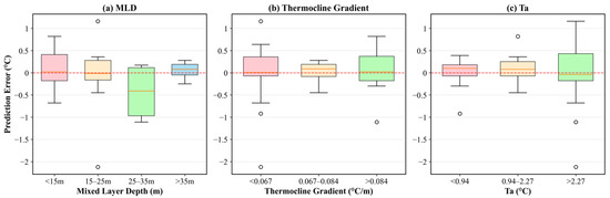
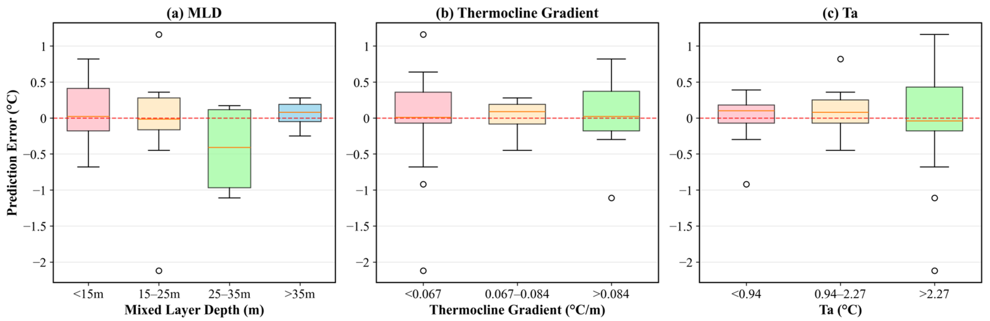
To further explore the sources of prediction errors, we selected MLD, thermocline gradient, and temperature anomaly ($T_a$) at different points near the tracks of six typical typhoons, and analyzed their relationship with prediction errors. As shown in Figure 16, the box plots reveal no linear relationship between these parameters and prediction errors. There is no simple increasing or decreasing trend. This indicates that the error distribution is highly nonlinear. The sources of error are complex and likely involve interactions among multiple factors, including typhoon intensity, translation speed, background ocean circulation, and ocean stratification.

Figure 16. Box plot distribution of prediction errors under different marine environmental parameters. The red dotted line indicates the zero-error reference line.

From Figure 16a, when MLD exceeds 35 m, the box height is lowest, meaning the errors are smallest. This suggests that the model performs more stably under deep mixed-layer conditions. In Figure 16b, prediction errors are smaller when the thermocline gradient is moderate (0.067–0.084 °C/m). When the stratification is either too strong (>0.084 °C/m) or too weak (<0.067 °C/m), the errors become larger. In Figure 16c, the smallest errors occur when the temperature anomaly ($T_a$) is below 0.94 °C, and errors increase substantially when T_a exceeds 2.27 °C. Overall, the model achieves better prediction accuracy when the mixed layer is deep, the thermocline gradient is moderate, and the temperature anomaly is small—that is, when the initial ocean stratification is relatively stable. This is consistent with the error analysis results presented earlier.

4. Discussion

The results above show that the MLP model performs well overall in predicting typhoon-induced SSC, but it has biases under certain conditions. In areas with a shallow mixed layer and a weak thermocline gradient, the model tends to underestimate cooling. A shallow mixed layer means the upper ocean holds less heat and responds more easily to wind stress. When the thermocline is weak, vertical mixing is stronger, which increases entrainment and upwelling. However, the model inputs do not directly represent vertical entrainment efficiency. They only use MLD and the thermocline gradient as indirect indicators. Extreme cooling events are rare in the training set, making it difficult for the model to accurately predict such cases, which leads to underestimation. In shallow shelf areas, the model tends to overestimate cooling. This is mainly because the training data come mostly from the open ocean. In deep water, most of the wind stress energy goes into vertical mixing, and bottom friction is negligible. In shallow water, part of this energy is lost to bottom friction, and horizontal transport redistributes the rest. This weakens vertical mixing. The model was built based on open-ocean physics and does not include water depth or bottom friction. As a result, it cannot fully capture the effect of seafloor topography on mixing. When a typhoon rapidly intensifies or weakens, the prediction errors become larger. This is because the model inputs are static. The model uses pre-storm background conditions and variables at the time of peak forcing, but it does not track how typhoon intensity or movement speed changes over time. When the storm turns sharply or its strength changes quickly, the inputs cannot reflect the evolving forcing. Overall, the model works well in deep, open water with moderate stratification. It can be used for fast forecasting or as a simple alternative to complex coupled models. However, it still has limitations in shallow water, under extreme stratification, and during rapid changes in typhoon structure. Users should consider these conditions when applying the model. Future work could include variables such as water depth and the rate of change in typhoon intensity to improve predictions under complex conditions.

5. Conclusions

This study developed an MLP-based model to predict sea surface cooling (SSC) during typhoon passage. The model has two main innovations. First, it directly predicts SSC instead of first predicting SST and then calculating cooling, which avoids error accumulation. Second, it uses instantaneous variables at the time of maximum wind speed as inputs, including wind fields, SLA, and 100 m water temperature at that moment. Tests on 46 independent typhoon cases show that the predicted SSC spatial distribution agrees well with observations and captures the typical rightward bias of cooling. SHAP analysis identifies meridional wind (vwnd_max, vwnd_0) and initial MLD (mld_0) as the most important predictors, and their positive or negative effects are consistent with physical understanding. Error analysis shows that the model performs best in open deep water with moderate stratification. It tends to underestimate strong cooling in areas with shallow mixed layers and weak thermocline gradients, overestimate cooling over shallow shelves, and produce larger errors when typhoons change direction or intensity rapidly. Boxplot analysis further confirms that prediction accuracy is higher in regions with stable stratification. The model requires only nine input variables and is computationally efficient. It can serve as an efficient tool for typhoon–ocean coupling forecasts. Its error patterns also provide useful information for improving mixed-layer parameterization. There is still room for improvement in complex ocean environments and under rapid changes in typhoon structure. Future work may consider adding dynamic features, time series models, or water depth as inputs.

References

- Wentz, F.J.; Gentemann, C.; Smith, D.; Chelton, D. Satellite Measurements of Sea Surface Temperature through Clouds. Science 2000, 288, 847–850. [Google Scholar] [CrossRef] [Scilit]
- Monaldo, F.M.; Sikora, T.D.; Babin, S.M.; Sterner, R.E. Satellite imagery of sea surface temperature cooling in the wake of hurricane edouard (1996). Mon. Weather Rev. 1997, 125, 2716–2721. [Google Scholar] [CrossRef] [Scilit]
- Price, J.F. Upper Ocean Response to a Hurricane. J. Phys. Oceanogr. 1981, 11, 153–175. [Google Scholar] [CrossRef] [Scilit]
- Lin, I.-I.; Liu, W.T.; Wu, C.; Chiang, J.C.H.; Sui, C. Satellite Observations of Modulation of Surface Winds by Typhoon-induced Upper Ocean Cooling. Geophys. Res. Lett. 2003, 30, 1131. [Google Scholar] [CrossRef] [Scilit]
- Shang, S.; Li, L.; Sun, F.; Wu, J.; Hu, C.; Chen, D.; Ning, X.; Qiu, Y.; Zhang, C.; Shang, S. Changes of Temperature and Bio-optical Properties in the South China Sea in Response to Typhoon Lingling, 2001. Geophys. Res. Lett. 2008, 35, L10602. [Google Scholar] [CrossRef] [Scilit]
- Chiang, T.-L.; Wu, C.-R.; Oey, L.-Y. Typhoon Kai-Tak: An Ocean’s Perfect Storm. J. Phys. Oceanogr. 2011, 41, 221–233. [Google Scholar] [CrossRef] [Scilit]
- Emanuel, K.A. An Air-Sea Interaction Theory for Tropical Cyclones. Part I: Steady-State Maintenance. J. Atmos. Sci. 1986, 43, 585–605. [Google Scholar] [CrossRef] [Scilit]
- Cione, J.J.; Uhlhorn, E.W. Sea Surface Temperature Variability in Hurricanes: Implications with Respect to Intensity Change. Mon. Weather Rev. 2003, 131, 1783–1796. [Google Scholar] [CrossRef] [Scilit]
- Wang, Y.; Wu, C.-C. Current Understanding of Tropical Cyclone Structure and Intensity Changes? A Review. Meteorol. Atmos. Phys. 2004, 87, 257–278. [Google Scholar] [CrossRef] [Scilit]
- Zhu, T.; Zhang, D.-L. The Impact of the Storm-Induced SST Cooling on Hurricane Intensity. Adv. Atmos. Sci. 2006, 23, 14–22. [Google Scholar] [CrossRef] [Scilit]
- Liu, X.; Wei, J.; Zhang, D.; Miller, W. Parameterizing Sea Surface Temperature Cooling Induced by Tropical Cyclones: 1. Theory and An Application to Typhoon Matsa (2005). J. Geophys. Res. Oceans 2019, 124, 1215–1231. [Google Scholar] [CrossRef] [Scilit]
- Black, W.J.; Dickey, T.D. Observations and Analyses of Upper Ocean Responses to Tropical Storms and Hurricanes in the Vicinity of Bermuda. J. Geophys. Res. Oceans 2008, 113, C08009. [Google Scholar] [CrossRef] [Scilit]
- Mei, W.; Pasquero, C. Spatial and Temporal Characterization of Sea Surface Temperature Response to Tropical Cyclones. J. Clim. 2013, 26, 3745–3765. [Google Scholar] [CrossRef] [Scilit]
- Yang, C.-Y.; Yang, Y.J.; Tseng, Y.-H.; Jan, S.; Chang, M.-H.; Wei, C.-L.; Terng, C.-T. Observational Evidence of Overlooked Downwelling Induced by Tropical Cyclones in the Open Ocean. Sci. Rep. 2024, 14, 335. [Google Scholar] [CrossRef] [Scilit]
- Ning, J.; Xu, Q.; Feng, T.; Zhang, H.; Wang, T. Upper Ocean Response to Two Sequential Tropical Cyclones over the Northwestern Pacific Ocean. Remote Sens. 2019, 11, 2431. [Google Scholar] [CrossRef] [Scilit]
- Cui, H.; Tang, D.; Mei, W.; Liu, H.; Sui, Y.; Gu, X. Predicting Tropical Cyclone-Induced Sea Surface Temperature Responses Using Machine Learning. Geophys. Res. Lett. 2023, 50, e2023GL104171. [Google Scholar] [CrossRef] [Scilit]
- Li, J.; Yang, Y.; Wang, G.; Cheng, H.; Sun, L. Enhanced Oceanic Environmental Responses and Feedbacks to Super Typhoon Nida (2009) during the Sudden-Turning Stage. Remote Sens. 2021, 13, 2648. [Google Scholar] [CrossRef] [Scilit]
- Wang, S.; Toumi, R. Recent Tropical Cyclone Changes Inferred from Ocean Surface Temperature Cold Wakes. Sci. Rep. 2021, 11, 22269. [Google Scholar] [CrossRef] [Scilit] [PubMed]
- Zhang, H.; He, H.; Zhang, W.-Z.; Tian, D. Upper Ocean Response to Tropical Cyclones: A Review. Geosci. Lett. 2021, 8, 1. [Google Scholar] [CrossRef] [Scilit]
- Tang, R.; Cai, L.; Yan, X.; Ye, X.; Xu, Y.; Yin, J. Study of the Response of Environmental Factors of the Coastal Area in Zhoushan Fishery to Typhoon In-Fa Based on Remote Sensing. Remote Sens. 2023, 15, 3349. [Google Scholar] [CrossRef] [Scilit]
- Liu, X.; Gu, Y.; Zhai, F.; Li, P.; Liu, Z.; Bai, P.; Liu, C.; Sun, L.; Wu, K. Dramatic Temperature Variations in the Yellow Sea during the Passage of Typhoon Lekima (2019). Estuar. Coast. Shelf Sci. 2022, 269, 107819. [Google Scholar] [CrossRef] [Scilit]
- Pham Thai, G.; Dang Thi, L.; Vu Thi Kieu, L.; Nguyen Thi Minh, N.; Pham Thi, T.; Tong Tran, H.; Dae Seong, J.; Kyungmin, H. Potential Risks of Climate Change and Tropical Storms on Ecosystem and Clams Culture Activities in Giao Thuy, Nam Dinh, Vietnam. Hum. Ecol. Risk Assess. 2023, 29, 836–858. [Google Scholar] [CrossRef] [Scilit]
- Wu, R.; Zhang, H.; Chen, D.; Li, C.; Lin, J. Impact of Typhoon Kalmaegi (2014) on the South China Sea: Simulations Using a Fully Coupled Atmosphere-Ocean-Wave Model. Ocean Model. 2018, 131, 132–151. [Google Scholar] [CrossRef] [Scilit]
- Lok, C.C.F.; Chan, J.C.L.; Toumi, R. Importance of Air-Sea Coupling in Simulating Tropical Cyclone Intensity at Landfall. Adv. Atmos. Sci. 2022, 39, 1777–1786. [Google Scholar] [CrossRef] [Scilit]
- Corale, L.; Malardel, S.; Bielli, S.; Bouin, M. Evaluation of a Mesoscale Coupled Ocean-atmosphere Configuration for Tropical Cyclone Forecasting in the South West Indian Ocean Basin. Earth Space Sci. 2023, 10, e2022EA002584. [Google Scholar] [CrossRef] [Scilit]
- Kim, H.-S.; Liu, B.; Thomas, B.; Rosen, D.; Wang, W.; Hazelton, A.; Zhang, Z.; Zhang, X.; Mehra, A. Ocean Component of the First Operational Version of Hurricane Analysis and Forecast System: Evaluation of HYbrid Coordinate Ocean Model and Hurricane Feedback Forecasts. Front. Earth Sci. 2024, 12, 1399409. [Google Scholar] [CrossRef] [Scilit]
- Vincent, E.M.; Lengaigne, M.; Madec, G.; Vialard, J.; Samson, G.; Jourdain, N.C.; Menkes, C.E.; Jullien, S. Processes Setting the Characteristics of Sea Surface Cooling Induced by Tropical Cyclones. J. Geophys. Res. Oceans 2012, 117, C02020. [Google Scholar] [CrossRef] [Scilit]
- Yin, X.; Wang, Z.; Liu, Y.; Xu, Y. Ocean Response to Typhoon Ketsana Traveling over the Northwest Pacific and a Numerical Model Approach. Geophys. Res. Lett. 2007, 34, L21606. [Google Scholar] [CrossRef] [Scilit]
- Wei, J.; Liu, X.; Jiang, G. Parameterizing Sea Surface Temperature Cooling Induced by Tropical Cyclones Using a Multivariate Linear Regression Model. Acta Oceanol. Sin. 2018, 37, 1–10. [Google Scholar] [CrossRef] [Scilit]
- Wada, A.; Uehara, T.; Ishizaki, S. Typhoon-Induced Sea Surface Cooling during the 2011 and 2012 Typhoon Seasons: Observational Evidence and Numerical Investigations of the Sea Surface Cooling Effect Using Typhoon Simulations. Prog. Earth Planet. Sci. 2014, 1, 11. [Google Scholar] [CrossRef] [Scilit]
- Wada, A. Numerical Simulations of Sea Surface Cooling by a Mixed Layer Model during the Passage of Typhoon Rex. J. Oceanogr. 2005, 61, 41–57. [Google Scholar] [CrossRef] [Scilit]
- Zhang, H.; Jing, M.; Zhang, H.; Li, L.; Zheng, Y.; Tang, J.; Tian, D.; Zhu, Y. Deep Learning Approach for Forecasting Sea Surface Temperature Response to Tropical Cyclones in the Western North Pacific. Deep Sea Res. Part Oceanogr. Res. Pap. 2023, 197, 104042. [Google Scholar] [CrossRef] [Scilit]
- Shao, Q.; Li, W.; Han, G.; Hou, G.; Liu, S.; Gong, Y.; Qu, P. A Deep Learning Model for Forecasting Sea Surface Height Anomalies and Temperatures in the South China Sea. J. Geophys. Res. Oceans 2021, 126, e2021JC017515. [Google Scholar] [CrossRef] [Scilit]
- Zhao, Z.; Zhou, J.; Du, H. Artificial Intelligence Powered Forecast of Oceanic Mesoscale Phenomena: A Typhoon Cold Wake Case Occurring in Northwest Pacific Ocean. Future Gener. Comput. Syst. 2022, 129, 389–398. [Google Scholar] [CrossRef] [Scilit]
- Wei, J.; Jiang, G.-Q.; Liu, X. Parameterization of Typhoon-Induced Ocean Cooling Using Temperature Equation and Machine Learning Algorithms: An Example of Typhoon Soulik (2013). Ocean Dyn. 2017, 67, 1179–1193. [Google Scholar] [CrossRef] [Scilit]
- Jiang, G.Q.; Xu, J.; Wei, J. A Deep Learning Algorithm of Neural Network for the Parameterization of Typhoon-Ocean Feedback in Typhoon Forecast Models. Geophys. Res. Lett. 2018, 45, 3706–3716. [Google Scholar] [CrossRef] [Scilit]
- Dare, R.A.; McBride, J.L. Sea Surface Temperature Response to Tropical Cyclones. Mon. Weather Rev. 2011, 139, 3798–3808. [Google Scholar] [CrossRef] [Scilit]
- Jiang, G.; Wei, J. A Parameterization Scheme for Typhoon-Ocean Interaction Based on a Deep Learning Neural Network. In IGARSS 2018—2018 IEEE International Geoscience and Remote Sensing Symposium; IEEE: New York, NY, USA, 2018; pp. 4419–4422. [Google Scholar] [CrossRef] [Scilit]
- Price, J.F. Metrics of Hurricane-Ocean Interaction: Vertically-Integrated or Vertically-Averaged Ocean Temperature? Ocean Sci. 2009, 5, 351–368. [Google Scholar] [CrossRef] [Scilit]
- Song, D.; Xiang, L.; Guo, L.; Li, B. Estimating Typhoon-Induced Sea Surface Cooling Based upon Satellite Observations. Water 2020, 12, 3060. [Google Scholar] [CrossRef] [Scilit]
- Liu, Z.H.; Xu, J.P.; Zhu, B.K.; Sun, C.H.; Zhang, L.F. Upper ocean response to tropical cyclones in northwestern Pacific during 2001-2004 by Argo data. J. Trop. Oceanogr. 2006, 25, 1–8. (In Chinese) [Google Scholar]
- GB/T 19201–2006; Grade of Tropical Cyclones. Standardization Administration of China: Beijing, China, 2006.
- Guan, S.; Zhao, W.; Sun, L.; Zhou, C.; Liu, Z.; Hong, X.; Zhang, Y.; Tian, J.; Hou, Y. Tropical Cyclone-Induced Sea Surface Cooling over the Yellow Sea and Bohai Sea in the 2019 Pacific Typhoon Season. J. Mar. Syst. 2021, 217, 103509. [Google Scholar] [CrossRef] [Scilit]
- Yablonsky, R.; Ginis, I. Impact of a Warm Ocean Eddy’s Circulation on Hurricane-Induced Sea Surface Cooling with Implications for Hurricane Intensity. Mon. Weather Rev. 2013, 141, 997–1021. [Google Scholar] [CrossRef] [Scilit]
- Lu, Z.; Wang, G.; Shang, X. Response of a Preexisting Cyclonic Ocean Eddy to a Typhoon. J. Phys. Oceanogr. 2016, 46, 2403–2410. [Google Scholar] [CrossRef] [Scilit]
- Li, J.; Zhang, H.; Liu, S.; Wang, X.; Sun, L. The Response and Feedback of Ocean Mesoscale Eddies to Four Sequential Typhoons in 2014 Based on Multiple Satellite Observations and Argo Floats. Remote Sens. 2021, 13, 3805. [Google Scholar] [CrossRef] [Scilit]
- Ma, Z. A Study of the Interaction between Typhoon Francisco (2013) and a Cold-Core Eddy. Part I: Rapid Weakening. J. Atmos. Sci. 2020, 77, 355–377. [Google Scholar] [CrossRef] [Scilit]
- Qiu, C.; Liang, H.; Sun, X.; Mao, H.; Wang, D.; Yi, Z.; Wirasatriya, A. Extreme Sea-Surface Cooling Induced by Eddy Heat Advection during Tropical Cyclone in the North Western Pacific Ocean. Front. Mar. Sci. 2021, 8, 726306. [Google Scholar] [CrossRef] [Scilit]
- Chelton, D.B.; Schlax, M.G.; Samelson, R.M. Global Observations of Nonlinear Mesoscale Eddies. Prog. Oceanogr. 2011, 91, 167–216. [Google Scholar] [CrossRef] [Scilit]
- Shang, X.; Zhu, H.; Chen, G.; Xu, C.; Yang, Q. Research on Cold Core Eddy Change and Phytoplankton Bloom Induced by Typhoons: Case Studies in the South China Sea. Adv. Meteorol. 2015, 2015, 340432. [Google Scholar] [CrossRef] [Scilit]
- Lu, X.; Yu, H.; Yang, X.; Li, X. Estimating Tropical Cyclone Size in the Northwestern Pacific from Geostationary Satellite Infrared Images. Remote Sens. 2017, 9, 728. [Google Scholar] [CrossRef] [Scilit]
- Lu, X.; Wong, W.; Yu, H.; Yang, X. Tropical Cyclone Size Identification over the Western North Pacific Using Support Vector Machine and General Regression Neural Network. J. Meteorol. Soc. Jpn. Ser. II 2022, 100, 927–941. [Google Scholar] [CrossRef] [Scilit]
Disclaimer/Publisher’s Note: The statements, opinions and data contained in all publications are solely those of the individual author(s) and contributor(s) and not of MDPI and/or the editor(s). MDPI and/or the editor(s) disclaim responsibility for any injury to people or property resulting from any ideas, methods, instructions or products referred to in the content. |
© 2026 by the authors. Licensee MDPI, Basel, Switzerland. This article is an open access article distributed under the terms and conditions of the Creative Commons Attribution (CC BY) license.