Water Spectra Reconstruction for Sentinel-2 MSI: From Multispectral to Hyperspectral

Highlights

What are the main findings?

• Water spectra database with diverse optical water types was constructed by integrating spectra data from hyperspectral satellites and in situ measurements.
• Validation with in situ measurements demonstrates that spectral reconstruction effectively restores water spectral information for the missing bands of Sentinel-2.

What is the implication of the main finding?

• Demonstrating that expanding spectral dataset with hyperspectral satellite is a valid approach to enhance reconstruction accuracy across various optical water types.
• The restoration of spectral information via reconstruction significantly expands the application potential of multispectral satellite data in water color remote sensing.

Abstract

For studies utilizing methods such as water color parameter inversion and algal bloom classification, abundant spectral bands and high spectral resolution are of great significance. However, for multispectral satellite sensors that are not designed for water color studies (e.g., Sentinel-2 MSI), the number of bands in the visible–near-infrared range is limited, and lacks specific spectral bands with rich spectral information. Hyperspectral reconstruction of multispectral data based on hyperspectral remote sensing reflectance ($R_{rs}$) databases and machine learning algorithms have been proven to be a feasible solution. Based on the in situ measured $R_{rs}$ data, this study constructed a large-sample hyperspectral $R_{rs}$ database covering various optical water types using two Chinese hyperspectral satellites, and compared the spectral reconstruction accuracy of six machine learning algorithms. The results show that expanding the $R_{rs}$ database for model training by integrating hyperspectral satellite data can effectively improve the reconstruction accuracy in waters of different optical types. Comparisons with in situ measured hyperspectral $R_{rs}$ indicate that the reconstructed Sentinel-2 hyperspectral data achieve high accuracy, with the Spectral Angle Mapper (SAM) less than 5° and the correlation coefficient ($r$) higher than 0.7. Furthermore, the reconstructed data can effectively restore spectral information not captured by the original multispectral data, such as the suspended sediment $R_{rs}$ peak at 580 nm and the chlorophyll $R_{rs}$ valley at 680 nm. Through spectral reconstruction, the spectral resolution of Sentinel-2 can be maximized while retaining its advantages of fast revisit capability and high spatial resolution, thereby expanding its application potential in water color remote sensing.

1. Introduction

In water color remote sensing, spatial resolution, temporal resolution (revisit period), and spectral resolution (number of bands) are the fundamental parameters determining the application potential of a sensor. High-spatial resolution satellites with abundant spatial details (e.g., Gaofen-2 (GF-2) and Worldview) can be applied to studies such as urban micro-river water monitoring [1] and high-precision shoreline extraction [2]. Geostationary satellites with an extremely short revisit cycle (e.g., GOCI-II (Geostationary Ocean Color Imager II) and Himawari-8) are suitable for studies like algal bloom tracking [3,4] and sea surface current observation [5]. Hyperspectral satellites, such as PACE (Plankton, Aerosol, Cloud, ocean Ecosystem), HICO (Hyperspectral Imager for the Coastal Ocean), ZY1-02D (Ziyuan1-02D) AHSI (Advanced Hyperspectral Imager) and PRISMA (Hyperspectral Precursor and Application Mission), with the ability to obtain hundreds of spectral bands, can capture more refined spectral features, thus demonstrating enormous application potential in studies like accurate inversion of water color parameters [6], marine plastic debris identification [7], and algal bloom classification [8,9,10,11].

However, due to physical and technical constraints as well as cost limitations, trade-offs must be made among spatial resolution, temporal resolution, and spectral resolution [12,13]. Numerous studies have been dedicated to enhancing these parameters at the algorithmic level. For instance, super-resolution models such as SRCNN (Super-Resolution Convolutional Neural Network) improve the spatial resolution of low-resolution images by learning the texture information between low and high-resolution images [14,15]; spatiotemporal fusion models like STARFM (Spatial and Temporal Adaptive Reflectance Fusion Model) generate images with both rich texture information and a short time interval by fusing high-spatial and high-temporal resolution images [16,17]; and multi-source satellite data assimilation technology achieves higher observation frequency by integrating data from multiple satellite platforms as well as in situ measurements [18].

In inland water color remote sensing, Sentinel-2 satellites has been widely used in studies such as algal bloom monitoring [19], water area extraction [20], inversion of water depth [21] and water quality parameter [22], thanks to its short revisit cycle (less than 5 days), high spatial resolution (up to 10 m), and a relatively abundant spectral bands (13 bands). However, as it is not specifically designed for water color remote sensing, it lacks water color characteristic bands such as 412 nm, 620 nm, and 680 nm. Ocean color satellites like Sentinel-3 OLCI (Ocean and Land Colour Instrument) and GOCI-II are equipped with such bands, but their low spatial resolution limits their application in inland waters. Therefore, some studies have attempted to reconstruct missing bands based on the existing spectral bands with a linear regression model: Jiang et al. [23] established a linear regression model between 665 nm and 620 nm using a large amount of in situ $R_{rs}$ data to reconstruct the virtual 620 nm band from the 665 nm band of Sentinel-2 MSI (Multispectral Imager); Paulino et al. [24] generated eight virtual band images with 10 m resolution using a multiple regression model, relying on quasi-synchronous Sentinel-2 MSI and Sentinel-3 OLCI image pairs. Deep learning algorithms are also widely used for reconstruction of missing bands: Wang et al. [25] reconstructed the $R_{rs}$ of ultraviolet bands from visible bands based on deep learning models; Young et al. [26] generated 186-band high-resolution hyperspectral images by proposing a novel lightweight and interpretable Unfolding Adversarial Learning Network (UALNet), which reconstructs Sentinel-2 multispectral data into Airborne Visible–Infrared Imaging Spectrometer—Next Generation (AVIRIS-NG)-level hyperspectral data through adversarial unfolding and data-driven spectral regularization.

Based on in situ $R_{rs}$ datasets, using methods such as regression fitting or machine learning to predict missing bands is currently the most commonly used approach. However, due to the much more complex optical properties of inland waters and the scarcity of publicly available $R_{rs}$ datasets, it is challenging to construct a $R_{rs}$ dataset covering different optical types of waters to support such studies. Therefore, this study aims to establish a spectral reconstruction model for Sentinel-2 multispectral images by integrating hyperspectral satellite imagery and in situ $R_{rs}$ data, and evaluate its reconstruction accuracy based on in situ measurements. The structure of this article is arranged as follows: Section 2 introduces the in situ and satellite data used in this study, details of the data preprocessing method, and machine learning algorithms. Section 3 shows reconstruction results and validation with in situ data, while discussing the limitations and potential improvement of this study. Finally, conclusions are presented in Section 4.

2. Materials and Methods

2.1. Materials

2.1.1. In Situ $R_{rs}$ Data

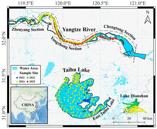
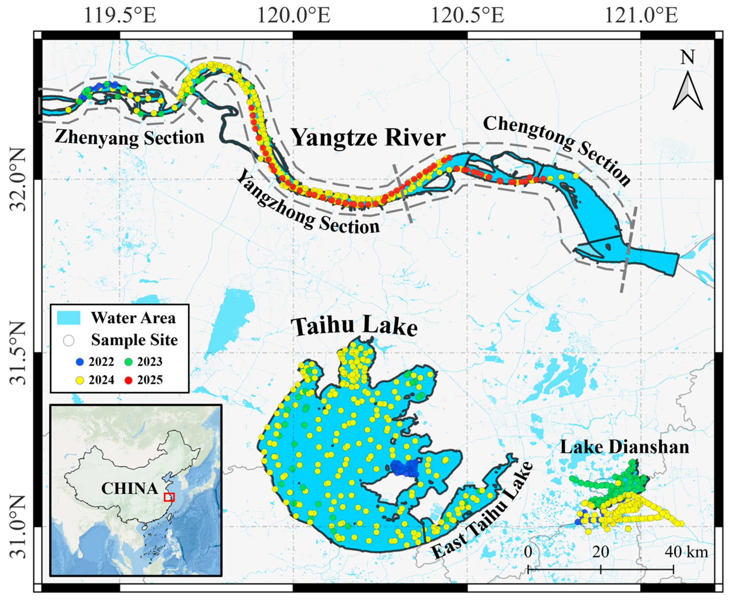
From 2022 to 2025, field sampling was performed in three typical water areas (the Yangtze River, Taihu Lake, and Lake Dianshan) of the Yangtze River Basin (Figure 1). The Yangtze River is a sediment-dominated river, whose sediment concentration exhibits significant variations between dry and flood seasons [27]. Taihu Lake is the third-largest freshwater lake in China, features an extremely shallow water depth (less than 2 m on average), suffers from severe eutrophication, and experiences frequent algal bloom events [28]. Lake Dianshan is the most important water source of Shanghai city, receives inflow from Taihu Lake in its upper reaches, and is subject to mild eutrophication with occasional algal blooms [29]. These three water bodies were selected in this study as they are typical representatives with distinct optical properties in the Yangtze River Basin, covering sediment-dominated rivers, severely eutrophic lakes, and mildly eutrophic lakes.

Figure 1. Location of research area and sampling sites. Dots with different colors represent sampling sites of different years.

All field sampling was conducted under clear sky conditions, and the period around noon with intense solar glint was avoided. In situ remote sensing reflectance ($R_{rs}$) data was measured using Triplet AOP (BRIGHTOCEAN TECH Co., Ltd., Guangzhou, China), an integrated apparent hyperspectrometer, strictly follows the “above-surface method” established by Mobley [30], which specified the observation direction of 40° from the nadir and 135 degrees from the sun. Water-leaving radiance, downwelling sky radiance, and downwelling solar irradiance were measured simultaneously, and in situ measured $R_{rs}$ was calculated by the following formula:

$$R_{rs}\left(\lambda \right)={\displaystyle \frac{L_u\left(\lambda \right)-r\times L_{sky}\left(\lambda \right)}{E_d\left(\lambda \right)}}$$

(1)

where $L_u\left(\lambda \right)$ is the water-leaving radiance, $L_{sky}\left(\lambda \right)$ is the downwelling sky radiance, $E_d\left(\lambda \right)$ is the total downwelling solar irradiance, and $r$ is the Fresnel reflectance of the water surface, empirically determined by the water surface wind speed during each day’s sampling. For calm water surfaces with negligible wind, $r$ was set to 0.022; for wind speeds of approximately 5 m/s and 10 m/s, $r$ was set to 0.025 and 0.028, respectively. After quality control, a total of 1307 hyperspectral $R_{rs}$ data were obtained, covering different water types such as turbid water, clear water, and algal bloom water; their locations are illustrated in Figure 1.

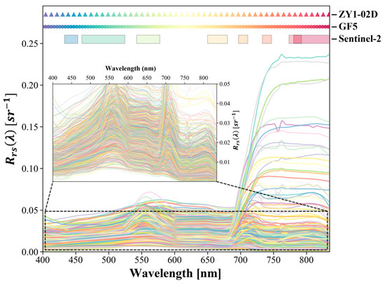
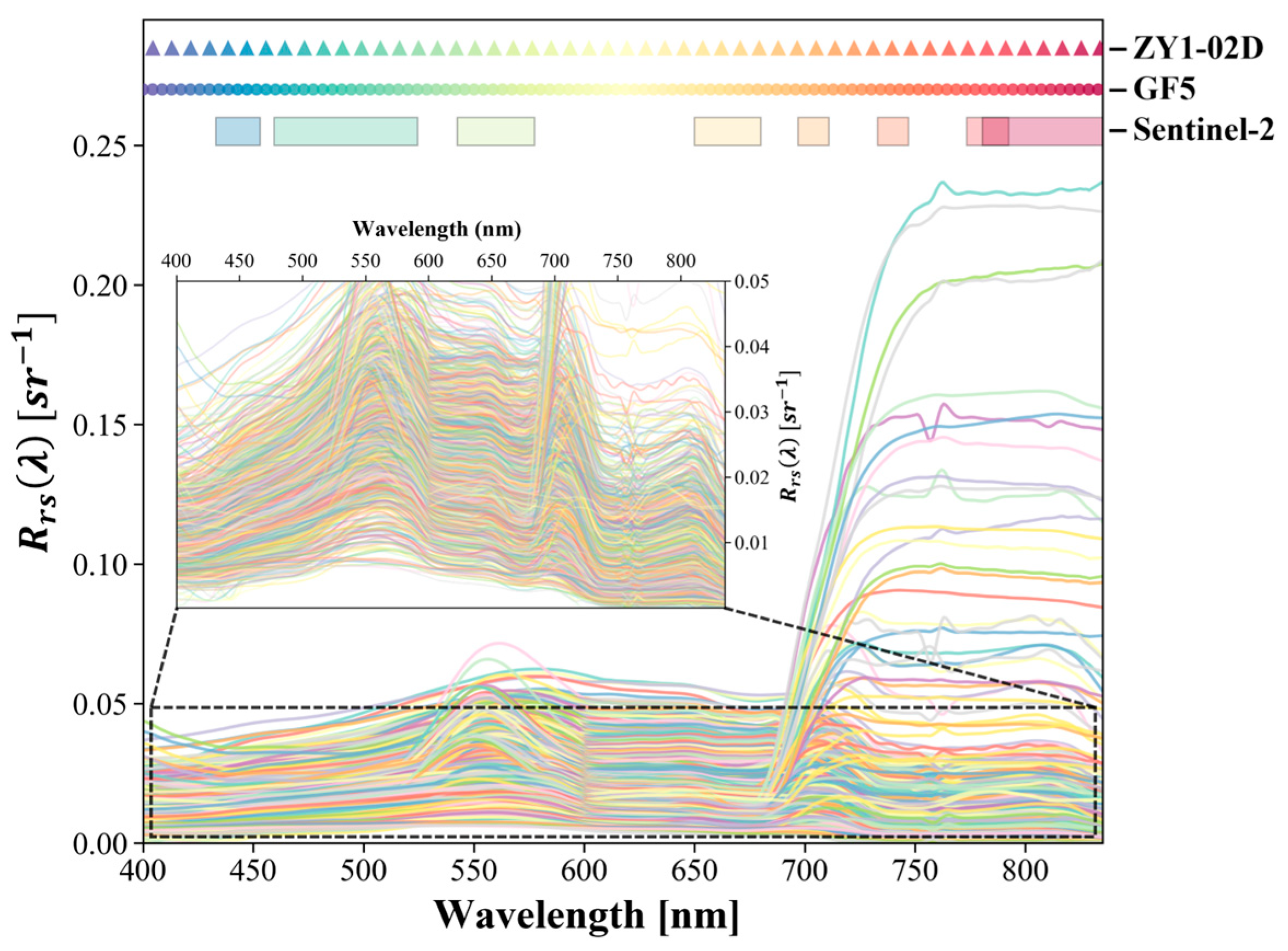
Since the Triplet AOP can only measure $R_{rs}$ data within the wavelength range of 400–830 nm, while the central wavelength of Sentinel-2 band 8 is 833 nm, linear extrapolation was performed on the in situ $R_{rs}$ to obtain data in the 831–835 nm range to match with Sentinel-2 bands. The spectra of in situ $R_{rs}$ are illustrated in Figure 2.

Figure 2. In situ $R_{rs}$ spectra and band setting of Sentinel-2 MSI, GF-5 and ZY1-02D AHSI (Advanced Hyperspectral Imager).

Furthermore, to reduce the influence of different band settings among various sensors, it is necessary to convert hyperspectral $R_{rs}$ data into equivalent $R_{rs}$ for each band of Sentinel-2 MSI, GF-5 AHSI and ZY1-02D, based on their Spectral Response Function (SRF) [31]. The calculation formula is as follows:

$$R_{\mathrm{r}\mathrm{s}}\left({\mathrm{band}}_i\right)={\displaystyle \frac{{\int }_{{\lambda }_1}^{{\lambda }_2} R_{\mathrm{r}\mathrm{s}}\left(\lambda \right)SRF\left(\lambda \right)d\left(\lambda \right)}{{\int }_{{\lambda }_1}^{{\lambda }_2} SRF\left(\lambda \right)d\left(\lambda \right)}}$$

(2)

where $R_{\mathrm{r}\mathrm{s}}\left({\mathrm{band}}_i\right)$ is the equivalent $R_{rs}$ of the $i$-th band of a specific satellite sensor, $[\lambda 1, \lambda 2]$ is the wavelength range of the band, $SRF\left(\lambda \right)$ is the spectral response of the sensor at wavelength $\lambda$, and $R_{\mathrm{r}\mathrm{s}}\left(\lambda \right)$ is the hyperspectral $R_{rs}$ at wavelength $\lambda$. During the validation of the atmospheric correction result, in situ measured hyperspectral $R_{rs}$ are converted into equivalent $R_{rs}$ of each satellite sensor, whereas during the construction of the input dataset of the reconstruction model, both hyperspectral $R_{rs}$ derived from in situ measurement and hyperspectral satellite sensor are converted into equivalent $R_{rs}$ of Sentinel-2 MSI.

For the MSI sensor onboard Sentinel-2 A/B/C, official SRFs of each multispectral band are available for download (https://sentiwiki.copernicus.eu/web/s2-documents, last accessed on 18 June 2025). For the AHSI sensor onboard GF-5 and ZY1-02D, SRFs were simulated based on the central wavelength and full width at half maxima (FWHM) of each band using a Gaussian function.

2.1.2. Hyperspectral Satellite Data and Preprocessing

Two Chinese hyperspectral satellites, GF-5 and ZY1-02D, were used in this study, both equipped with the AHSI that can acquire hyperspectral data in the 400–2500 nm range with different spectral band settings. Specific information of each sensor is presented in Table 1.

Table 1. Sensor information of Sentinel-2 MSI, GF-5 AHSI and ZY1-02D AHSI, where CW stands for central wavelength (nm), BR stands for band range (nm), BW stands for band width (nm), FWHM stands for full width at half maxima (nm), and SR stands for spatial resolution (m).

Parameters	Sentinel-2 MSI			GF-5 AHSI			ZY1-02D AHSI
Orbit Altitude (km)	786			705			778
Revisit cycle (d)	<5			5			3
Swath Width (km)	290			60			60
Spectral Bands	13 (VNIR: 10 SWIR: 3)			330 (VNIR: 150 SWIR: 180)			166 (VNIR: 76 SWIR: 90)
Date of Launch	23 June 2015 Sentinel-2A 7 March 2017 Sentinel-2B 5 September 2024 Sentinel-2C			7 September 2021 GF5-B 9 December 2022 GF5-01A			12 September 2019 ZY1-02D 16 December 2021 ZY1-02E
Spectral Info	CW	BW	SR	BR	FWHM	SR	BR	FWHM	SR
	443	20	60	390–1050	4.38	30	390–1050	8.76	30
	492	65	10
	560	35	10
	665	30	10
	704	15	20
	740	15	20
	783	20	20
	833	115	10
	865	20	20
	945	20	60
	1375	30	60	1000–2505	8.25		1000–2505	16.26
	1610	90	20
	2190	180	20

For the raw data of GF-5 and ZY1-02D, ENVI 6.0 software is used to perform radiometric calibration, atmospheric correction, and orthometric correction to obtain the geo-corrected $R_{rs}$ images. Atmospheric correction was performed using the FLAASH (Fast Line-of-sight Atmospheric Analysis of Hypercubes) module, a widely adopted method for hyperspectral satellite imagery in water color remote sensing [32,33,34]. The Automated Water Extraction Index ($AWEI$) was adopted to extract pure water pixels. Proposed by Feyisa et al. [35], $AWEI$ distinguishes water from land through a linear weighted combination of multiple bands based on the spectral characteristics of different ground objects. Its calculation formula is as follows:

$$AWEI=4\times \left({Rrs}_{Green}-{Rrs}_{SWIR1}\right)-\left(0.25\times {Rrs}_{NIR}+2.75\times {Rrs}_{SWIR2}\right)$$

(3)

where ${Rrs}_{Green}$, ${Rrs}_{NIR}$, ${Rrs}_{SWIR1}$ and ${Rrs}_{SWIR2}$ represent $R_{rs}$ of the green, near-infrared (NIR), and two shortwave infrared (SWIR) bands, respectively.

However, for algal bloom waters, ${Rrs}_{NIR}$ tends to be higher than clean water due to the strong scattering effect of floating algae in the NIR band, which penalizes the $AWEI$ calculation result and leads to a low value. Therefore, this study modified the $AWEI$ by removing the penalty term of the NIR band and increasing the penalty coefficient of the SWIR band. The calculation formula of the modified $AWEI$ (${AWEI}_{mod}$) is as follows:

$${AWEI}_{mod}=4\times \left({Rrs}_{Green}-{Rrs}_{SWIR1}\right)-3\times {Rrs}_{SWIR2}$$

(4)

For GF-5 and ZY1-02D images, the $R_{rs}$ values of the bands closest to 550 nm, 1530 nm, and 2200 nm of each sensor were selected as ${Rrs}_{Green}$, ${Rrs}_{SWIR1}$ and ${Rrs}_{SWIR2}$, respectively. Pixels with ${AWEI}_{mod}>0$ were considered water pixels. To minimize the mixed pixel effect caused by pixels such as shorelines and ships, an erosion operation was further performed on the water mask, ultimately achieving the extraction of pure water pixels.

2.1.3. Multispectral Satellite Data and Preprocessing

In this study, Sentinel-2 MSI images were used as the multispectral images to be reconstructed; sensor information is presented in Table 1. Level-1C Top-of-Atmosphere (TOA) radiance products were downloaded from the Copernicus Data Space Ecosystem (https://dataspace.copernicus.eu/, last accessed on 11 September 2025), and $R_{rs}$ data were obtained using the ACOLITE (v20260421.0) atmospheric correction software. ACOLITE is an open-source atmospheric correction software specifically designed for coastal and inland turbid waters [36], supporting various medium-to-high spatial resolution remote sensing images, including Sentinel-2 MSI and Landsat OLI [37]. Based on the Dark Spectrum Fitting (DSF) atmospheric correction algorithm [38,39], it achieves high accuracy in turbid waters such as coastal and inland areas [40,41,42,43,44]. Due to the inconsistent spatial resolutions of different Sentinel-2 bands, they were uniformly resampled to 10 m after atmospheric correction. After obtaining the $R_{rs}$ data, 8 of its bands within the 400–835 nm range were used as input data for the spectral reconstruction model.

2.2. Methods

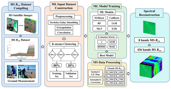
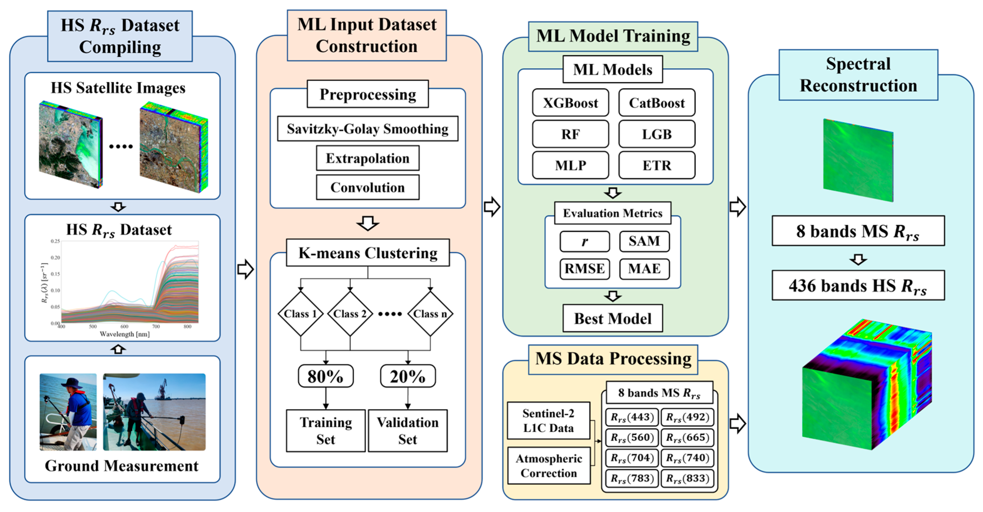
The technical workflow of this study is illustrated in Figure 3. Firstly, preprocessing was performed on the in situ data and hyperspectral images to obtain a hyperspectral $R_{rs}$ dataset. After further processing (smoothing, convolution, K-means clustering, and so on), the dataset, a machine learning input dataset, was established. Subsequently, the optimal model was selected based on accuracy evaluation metrics, including the Spectral Angle Mapper (SAM) and correlation coefficient ($r$). Finally, the eight-band Sentinel-2 multispectral $R_{rs}$ was reconstructed into a 436-band hyperspectral $R_{rs}$, and was cross-validated with in situ and satellite data.

Figure 3. Workflow of Sentinel-2 MSI $R_{rs}$ reconstruction, where HS stands for hyperspectral, MS stands for multispectral, and ML stands for machine learning.

2.2.1. $R_{rs}$ Dataset Extraction from Hyperspectral Satellite

For the preprocessed hyperspectral satellite data, the Savitzky–Golay filter [45] was employed to smooth and denoise the $R_{rs}$ data. By performing low-order polynomial least squares fitting on equally spaced data points within a sliding window, it can accurately retain key spectral features such as peak position, width, and height while suppressing high-frequency noise. Subsequently, due to the mismatch between its spectral resolution (GF-5: 4.38 nm, ZY1-02D: 8.76 nm) and the in situ hyperspectral data (1 nm), linear interpolation was first performed on the satellite-derived $R_{rs}$ data to generate 1 nm interval $R_{rs}$ data in the 400–835 nm range.

Each hyperspectral image contains nearly one million water pixels. In order to remove redundant information and extract representative water spectra from different water types covered by the images, this study used K-means clustering [46] for cluster sampling of the preprocessed hyperspectral $R_{rs}$. Its core idea is to partition the dataset into K disjoint clusters through iterative optimization, maximizing the similarity of samples within the same cluster and minimizing the similarity of samples between different clusters. K-means clustering can effectively explore the inherent characteristic laws of spectral curves and has been widely applied in studies on water optical classification based on $R_{rs}$ [47,48,49].

Considering that hyperspectral images with different imaging ranges cover different water areas, this study automatically selected the optimal number of clusters by calculating the silhouette coefficient [50]. For a specified number of water spectrum extractions, after automatically determining the number of clusters, to avoid uneven distribution of extraction quantities caused by larger clusters of water pixels obtaining more extractions, an adaptive weighted sampling strategy was adopted instead of a proportional sampling strategy based on the proportion of each water type, ensuring that water types with a smaller proportion can obtain a relatively higher number of samples. The calculation method is as follows:

$$W_i={\displaystyle \frac{\alpha }{C_i}}+(1-\alpha )\times C_i$$

(5)

$$N_i={\displaystyle \frac{N_{sum}\times W_i}{W_{sum}}}$$

(6)

where $W_i$ is the weight of the $i$-th water cluster, $C_i$ is the proportion of the $i$-th water cluster, and $\alpha$ is the weighting coefficient, set to 0.1 in this study. $N_i$ is the number of samples drawn from a specific water type, $W_{sum}$ is the total weight, and $N_{sum}$ is the specified total number of samples drawn per image, set to 1000 to avoid data redundancy. After determining the sampling quantity for each water type, random sampling was performed within each water cluster, ultimately obtaining the specified number of water spectra.

2.2.2. Machine Learning Models

Six classic machine learning models were tested in this study to reconstruct hyperspectral $R_{rs}$ from multispectral data, including the following: two random tree ensemble models: RF and ETR; three Gradient Boosting Decision Tree models: LightGBM, XGBoost and CatBoost; and the neural network model MLP.

RF (Random Forest Regressor) [51] is an ensemble learning algorithm. It generates multiple training subsets through “Bootstrap sampling”, trains a decision tree for each subset (only using randomly sampled features when splitting nodes), and finally averages the prediction results of all trees for regression tasks. The strategy of “sampling + random feature selection” reduces the overfitting risk of individual trees and balances accuracy and generalization ability.

ETR (Extremely Randomized Trees Regressor) [52] is an extended variant of Random Forest and belongs to the ensemble learning model, using unpruned decision trees as base predictors. Its core feature is enhancing the randomness of tree construction: when building each node, it does not search for the optimal splitting threshold but randomly generates thresholds for candidate features, then selects the threshold that minimizes the regression loss to split the node. Meanwhile, it combines feature sampling (only using part of the features for each node) to reduce the correlation between base trees and improve the model’s generalization ability.

LightGBM (Light Gradient Boosting Machine Regressor) [53] is a lightweight GBDT (Gradient Boosting Decision Tree) framework. Its core optimizations include Gradient-based One-Side Sampling (GOSS) and Exclusive Feature Bundling (EFB): GOSS samples large-gradient samples and some small-gradient samples to reduce computational complexity; EFB bundles mutually exclusive features into “feature bundles” to reduce feature dimensionality. It also adopts a “leaf-wise growth” strategy (prioritizing expanding leaf nodes with the largest loss) to improve accuracy with fewer trees.

XGBoost (Extreme Gradient Boosting Regressor) [54] is an optimized GBDT framework. Its core improvements include a second-order Taylor expansion of the loss function and regularization: expanding the loss function to the second-order term improves the accuracy of gradient estimation, and introducing a regularization term to penalize tree complexity to suppress overfitting. It uses a “weighted quantile sketch” to optimize the search for splitting thresholds and supports parallel computing.

CatBoost [55] is a GBDT optimized for datasets containing categorical features. Its core innovations are categorical feature processing and ordered boosting: it encodes categorical features through “category-label mean” and introduces prior values to avoid training leakage; it optimizes gradient estimation by randomly permuting the dataset and uses “oblivious trees” (nodes at the same depth use the same splitting threshold) to suppress overfitting.

MLP (Multilayer Perceptron Regressor) [56] is a classic feedforward neural network composed of an input layer, hidden layers, and an output layer. Features are transmitted through weighted connections, nonlinear activation functions (e.g., ReLU) are used in hidden layers to introduce nonlinearity, and linear activation functions are used in the output layer to output regression results; weights are updated by minimizing loss through the backpropagation algorithm.

2.2.3. Accuracy Evaluation Metrics

Following previous studies [57,58,59,60], to evaluate the reconstruction performance both in the spectral scale and numerical scale, the spectral similarity between the true and reconstructed $R_{rs}$ was calculated based on the correlation coefficient ($r$) and Spectral Angle Mapper (SAM), while errors were quantified using the Root Mean Square Error (RMSE) and Mean Absolute Error (MAE).

(1)

Correlation coefficient ($r$)

Measures the linear correlation between two sets of $R_{rs}$ data with a value range of [−1, 1]. A value closer to 1 indicates a stronger linear correlation and better consistency in the overall spectral trend:

$$r={\displaystyle \frac{\sum _{i=1}^n \sum _{j=1}^m \left(y_{\mathrm{true}, i,j}-{\overline{y}}_{\mathrm{true} }\right)\left(y_{\mathrm{pred},i,j}-{\overline{y}}_{\mathrm{pred} }\right)}{\sqrt{\sum _{i=1}^n \sum _{j=1}^m {\left(y_{\mathrm{true},i,j}-{\overline{y}}_{\mathrm{true} }\right)}^2}\cdot \sqrt{\sum _{i=1}^n \sum _{j=1}^m {\left(y_{\mathrm{pred},i,j}-{\overline{y}}_{\mathrm{pred} }\right)}^2}}}$$

(7)

where $y_{\mathrm{true},i,j}$ is the true $R_{rs}$ of the $j$-th band of the $i$-th sample, $y_{\mathrm{pred},i,j}$ is the corresponding predicted $R_{rs}$, and ${\overline{y}}_{\mathrm{true} }$ and ${\overline{y}}_{\mathrm{pred}}$ are the overall means of the true and predicted $R_{rs}$, respectively.

(2)

Spectral Angle Mapper (SAM)

Measures the directional similarity of two spectral vectors of a single sample in high-dimensional space, with the unit of degrees (°). A value closer to 0 indicates a more consistent spectral shape, and it is not affected by differences in $R_{rs}$ values:

$$\mathrm{S}\mathrm{A}\mathrm{M}\left({\mathit{y}}_{\mathrm{true},i},{\mathit{y}}_{\mathrm{pred},i}\right)={\displaystyle \frac{{180}^{\circ }}{\pi }}\cdot \arccos \left({\displaystyle \frac{{\mathit{y}}_{\mathrm{true},i}\cdot {\mathit{y}}_{\mathrm{pred},i}}{‖{\mathit{y}}_{\mathrm{true},i}‖\cdot ‖{\mathit{y}}_{\mathrm{pred},i}‖}}\right)$$

(8)

where ${\mathit{y}}_{\mathrm{true},i}$ and ${\mathit{y}}_{\mathrm{pred},i}$ are the true and predicted spectral vectors of the $i$-th sample; $\cdot$ denotes the vector dot product, and $‖\cdot ‖$ denotes the vector L2 norm.

(3)

Root Mean Square Error (RMSE) and Mean Absolute Error (MAE)

RMSE and MAE measure the mean of squared deviations and the absolute deviation degree between two sets of $R_{rs}$ data, reflecting extreme deviations and average deviation in the data, with the same unit as $R_{rs}$ (sr⁻¹). A smaller RMSE and MAE indicate smaller deviations and fewer extreme errors:

$$\mathrm{R}\mathrm{M}\mathrm{S}\mathrm{E}=\sqrt{{\displaystyle \frac{1}{n\cdot m}}\sum _{i=1}^n \sum _{j=1}^m {\left(y_{\mathrm{t}\mathrm{r}\mathrm{u}\mathrm{e},i,j}-y_{\mathrm{p}\mathrm{r}\mathrm{e}\mathrm{d},i,j}\right)}^2}$$

(9)

$$\mathrm{AE} ={\displaystyle \frac{1}{n\cdot m}}\sum _{i=1}^n \sum _{j=1}^m \left|y_{\mathrm{true},i,j}-y_{\mathrm{pred},i,j}\right|$$

(10)

where ${\mathit{y}}_{\mathrm{true},i,j}$ and ${\mathit{y}}_{\mathrm{pred},i,j}$ are the true and predicted $R_{rs}$ of the $j$-th band of the $i$-th sample.

3. Results and Discussion

3.1. Validation of Satellite Derived $R_{rs}$ Data

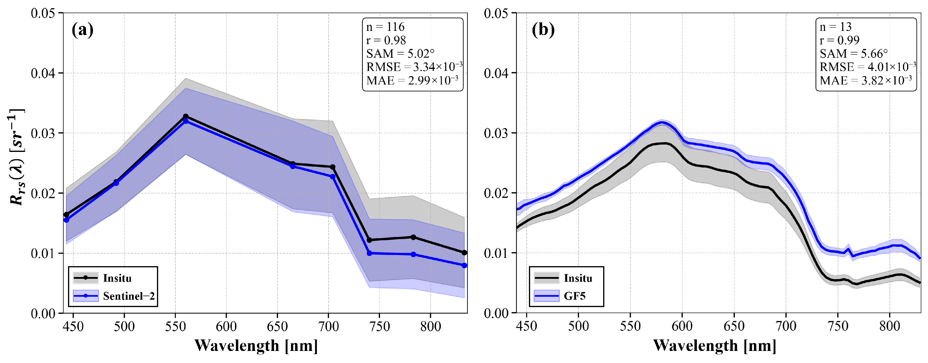
Accuracy of Sentinel-2 MSI and GF-5 AHSI atmospheric corrected $R_{rs}$ was validated with in situ measured $R_{rs}$. Firstly, considering the short-term variability of water bodies within the study area, the in situ $R_{rs}$ within a short time window of ±1.5 h around the satellite overpass time were converted using Equation (2) to obtain band equivalent $R_{rs}$. Satellite $R_{rs}$, within a 3 × 3 pixel window centered on the pixel where the sampling point was located, was averaged to serve as the satellite-derived $R_{rs}$ corresponding to the sampling point.

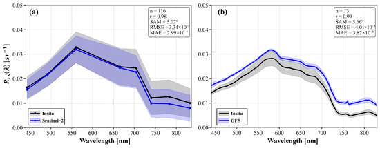
The accuracy evaluation results of Sentinel-2 $R_{rs}$ are shown in Figure 4a. It can be seen that the 116 in situ spectra covering different water areas and seasons have an average $r$ of up to 0.98, and the average RMSE and MAE are only 0.0033 sr⁻¹ and 0.0030 sr⁻¹, respectively, indicating that the ACOLITE atmospheric correction algorithm achieves high accuracy. The verification results of GF-5 $R_{rs}$ are presented in Figure 4b, the results are slightly higher in value than the in situ measurements, with an average RMSE of 0.0040 sr⁻¹ and MAE of 0.0038 sr⁻¹. The spectral shapes of the atmospheric correction results from both sensors are extremely close to the in situ values, with average SAM values of only 5.02° and 5.66°, respectively, and $r$ both greater than 0.98. Overall, although there are minor numerical deviations between the $R_{rs}$ spectra obtained by satellite sensors and the in situ $R_{rs}$, they can all restore the spectral shapes of various water types well.

Figure 4. Atmospheric correction results evaluation of satellite sensors. (a) Sentinel-2 and (b) GF-5.

3.2. Construction of Hyperspectral $R_{rs}$ Input Dataset

To ensure the accuracy of $R_{rs}$ extracted from hyperspectral satellite images, only high-quality images with absolutely no clouds and no stripes were used for cluster sampling to expand the $R_{rs}$ database. After quality control, a total of 6768 water spectra were finally extracted from hyperspectral satellite images, covering different water types such as turbid water, clear water, and algal bloom water.

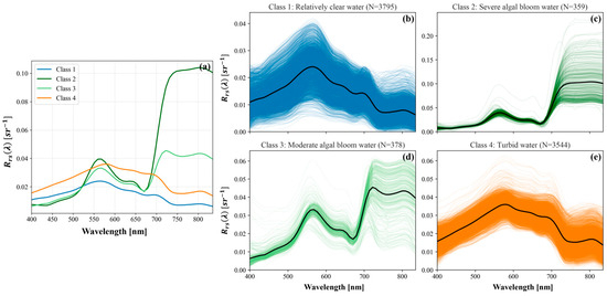
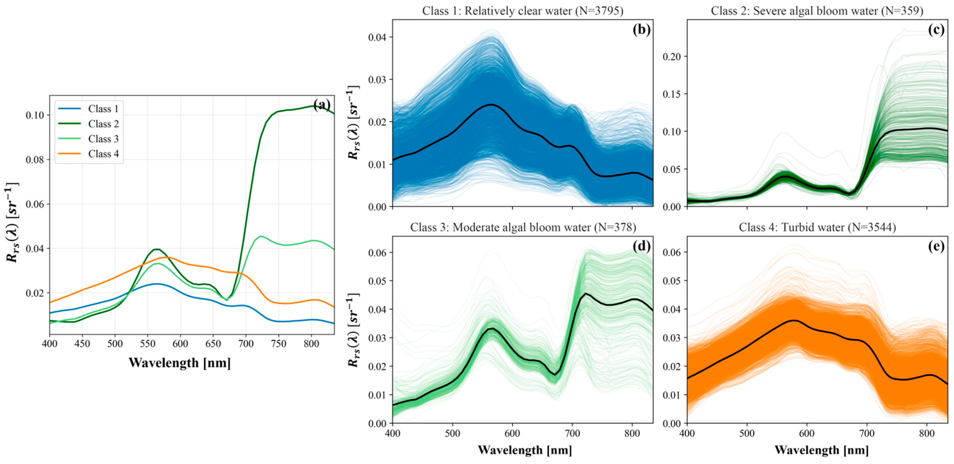
After expanding the $R_{rs}$ database based on hyperspectral satellite images, to construct the input dataset for the machine learning model, K-means clustering analysis was performed again on the expanded database, with the first-order derivative of $R_{rs}$ as input. Four different water classes were obtained, and their average spectral curves and the spectral curves of each water type are shown in Figure 5. Based on previous studies [49,61], the clustering results can be divided into four categories: Class 1 (Figure 5b) represents relatively clear water with low sediment and chlorophyll concentration, and there is a $R_{rs}$ peak around 700 nm determined by the algae concentration. $R_{rs}$ of this type of water are generally between 0 and 0.03 sr⁻¹; the clearer the water, the lower the $R_{rs}$ value, and the near-infrared band has the lowest $R_{rs}$ due to water absorption. Class 2 (Figure 5c) represents severe algal bloom water; due to the strong scattering effect of phytoplankton in the 700–835 nm band, its $R_{rs}$ soars in the red to near-infrared bands, with an average of up to 0.10 sr⁻¹. In the blue–violet band of 400–450 nm, due to the strong absorption of chlorophyll a, its $R_{rs}$ value is lower than that of normal water, only about 0.005 sr⁻¹. Class 3 (Figure 5d) represents moderate algal bloom water, with spectral characteristics similar to those of severe algal bloom water, both showing high near-infrared and low blue–violet $R_{rs}$ values, but these characteristics are weakened due to the lower algae concentration. Its $R_{rs}$ is generally in the range of [0, 0.05], and the high value in the near-infrared band gradually decreases with the reduction in algae concentration, but there is still a significant $R_{rs}$ peak at 710 nm. Class 4 (Figure 5e) represents water dominated by non-pigmented particles, mainly turbid water with high sediment concentration. The overall $R_{rs}$ of this type of water is higher than that of clear water, ranging from 0.01 to 0.04 sr⁻¹. Due to strong backscattering and weak absorption of non-pigmented particulate matter, it has a high $R_{rs}$ in the red band, and as the sediment concentration increases, a second $R_{rs}$ peak gradually appears near 790–820 nm.

Figure 5. Clustering result of $R_{rs}$ dataset. (a) Average $R_{rs}$ spectra of each class. (b–e) Full $R_{rs}$ spectra of each class.

The statistics of the number of various water spectra before and after the expansion of the $R_{rs}$ database based on hyperspectral satellite $R_{rs}$ are shown in Table 2. Before adding the hyperspectral satellite $R_{rs}$, there were only 79 in situ algal bloom water datasets in total. The small sample size may lead to problems such as overfitting and insufficient generalization ability during the training of machine learning models, making it difficult to accurately capture the differences in spectral characteristics of algal bloom water with different degrees, thereby affecting the classification accuracy and stability of the model in practical applications. After adding the hyperspectral satellite $R_{rs}$, the spectral data of algal bloom water has been greatly expanded. The spectral data volume of severe algal bloom water (Class 2) and moderate algal bloom water (Class 3) has increased by 1138% and 656%, respectively, which has greatly enriched the sample size and provided more sufficient training and verification data support for machine learning models.

Table 2. Data volume of each class.

Data Source	Class 1	Class 2	Class 3	Class 4
Insitu	641	29	50	588
Insitu + Satellite	3795	359	378	3544

3.3. Machine Learning Model Training

The expanded $R_{rs}$ database was divided into a training set and a validation set according to cluster types, with 80% used for model training and 20% for model validation. Six mainstream machine learning models, namely ETR, Random Forest (RF), CatBoost (CAT), LightGBM (LGB), XGBoost (XGB) and MLP, were trained respectively. GridSearchCV was adopted for each model to automatically determine the optimal hyperparameters in order to improve the models’ performance and avoid overfitting. Regularization terms and early stopping strategies were also applied in Gradient Boosting-based and neural network-based models. The reconstruction accuracy of their training results on different water types is presented in Table 3.

Table 3. Accuracy evaluation results of different machine learning algorithms.

Model	Class	SAM (°)	$\mathit{r}$	RMSE (×10−5)	MAE (×10−5)
CAT	1	1.6534	0.9980	4.6477	3.1639
ETR		1.1607	0.9989	3.4735	2.0102
LGB		1.3646	0.9986	3.9056	2.4167
MLP		1.7982	0.9977	4.9716	3.3985
RF		1.2681	0.9987	3.7305	2.2013
XGB		1.2580	0.9988	3.6367	2.1849
CAT	2	1.1589	0.9946	43.9402	13.7288
ETR		0.6836	0.9975	19.8908	6.2014
LGB		1.1496	0.9941	46.9167	15.3107
MLP		0.7122	0.9996	12.6261	6.0474
RF		0.7395	0.9979	27.4800	6.5539
XGB		1.1200	0.9946	32.1250	9.0971
CAT	3	1.3101	0.9985	7.6956	4.8729
ETR		0.7929	0.9994	4.9655	2.5919
LGB		1.0004	0.9992	5.7919	3.6110
MLP		1.0733	0.9992	5.7689	3.7975
RF		0.9171	0.9992	5.4892	2.9163
XGB		0.9414	0.9992	5.6550	3.3782
CAT	4	0.9056	0.9985	4.7884	3.1392
ETR		0.6257	0.9993	3.3883	1.9201
LGB		0.7039	0.9990	3.8759	2.2926
MLP		0.9676	0.9985	4.7478	3.1948
RF		0.6718	0.9992	3.5988	2.0922
XGB		0.6526	0.9990	3.8588	2.1152
CAT	Mean	1.2570	0.9974	15.2680	6.2262
ETR		0.8157	0.9988	7.9295	3.1809
LGB		1.0546	0.9977	15.1225	5.9078
MLP		1.1378	0.9987	7.0286	4.1096
RF		0.8991	0.9988	10.0746	3.4409
XGB		0.9930	0.9979	11.3189	4.1938

It can be seen that the average $r$ of all models is higher than 0.99, and the SAM is generally less than 1.5°, indicating that all models can capture the overall trend of $R_{rs}$ well, and their spectral reconstruction results have a relatively consistent spectral shape with the true values. However, there are certain differences in the accuracy of different models on different water types. For Classes 1, 3, and 4, ETR performs optimally among all evaluation metrics. In Class 2 (severe algal bloom water), although ETR achieves the lowest SAM of only 0.6836°, MLP performs slightly better than ETR in terms of $r$, RMSE, and MAE. Overall, the ETR model exhibits the best performance across all water types, with an average SAM of only 0.8157°. In contrast, LightGBM and XGBoost show relatively poorer reconstruction accuracy, with the highest RMSE and MAE of approximately 15 × 10⁻⁴ sr⁻¹ and 6 × 10⁻⁴ sr⁻¹, respectively. It is noteworthy that for Class 2 (severe algal bloom water), all models yield the highest RMSE and MAE among the four water types, which may be related to the strong nonlinear fluctuations in the $R_{rs}$ spectra of severe algal bloom water, increasing the difficulty of the model in fitting its characteristics.

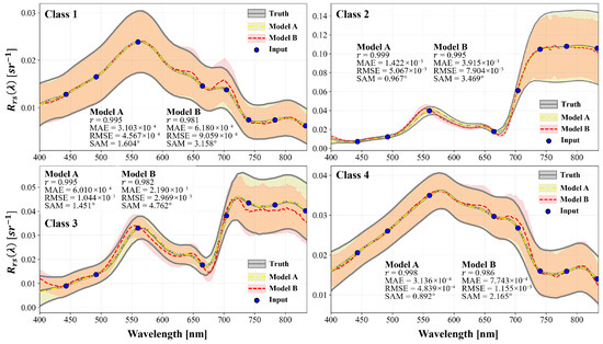
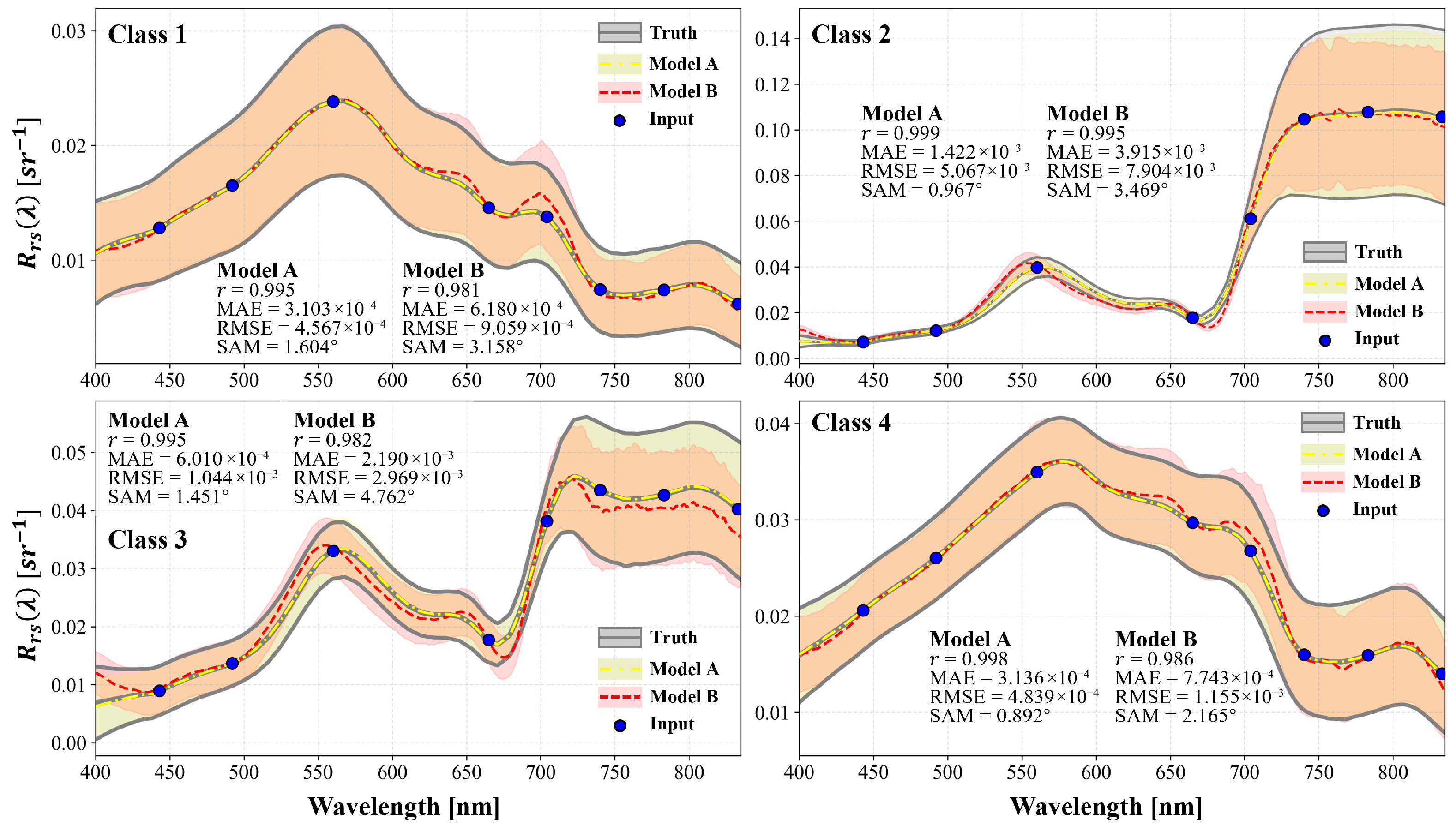
The ETR model with the best comprehensive performance was adopted for subsequent spectral reconstruction. To intuitively demonstrate the impact of expanding the database with the hyperspectral satellite $R_{rs}$ on the model’s reconstruction accuracy, two different models were trained based on the ETR model: Model A was trained using both in situ measurements and hyperspectral satellite $R_{rs}$ data, while Model B was trained solely with in situ $R_{rs}$. The training results of the two models were applied to the same test set, and their reconstruction effects on different water types are shown in Figure 6. It can be seen that the reconstruction results of Model B exhibit certain distortions in all water types. For Class 1 and Class 4, Model B achieves high reconstruction accuracy in the 450–600 nm range, but in the 600–835 nm range, it overestimates $R_{rs}$ at 630–720 nm and underestimates near 770 nm. In contrast, for algal bloom water (Class 2 and Class 3) with a small sample size, the reconstruction accuracy of Model B is significantly lower: it overestimates $R_{rs}$ at 400–440 nm, fails to accurately reconstruct the $R_{rs}$ peak near 560 nm and the $R_{rs}$ valley near 680 nm, and the reconstruction results for wavelengths greater than 710 nm show large fluctuations and significant deviations from the in situ data. Overall, the average SAM of Model B is 175.82% higher than that of Model A, and the RMSE is 83.42% higher, indicating that its reconstruction results are inferior to Model A in both spectral shape and numerical accuracy. In contrast, Model A, trained based on the expanded $R_{rs}$ database, achieves an average SAM of only 1.23° and an RMSE of 0.0018 sr⁻¹. Its average $R_{rs}$ curve and $\pm 1 \sigma$ interval are more consistent with the in situ data, demonstrating that the expansion of training samples has significantly improved the model’s adaptability and robustness to complex water scenarios.

Figure 6. Reconstruction result of different models: black line represents genuine $R_{rs}$ spectra, yellow dashed line represents reconstructed $R_{rs}$ of Model A (in situ and Satellite $R_{rs}$), and red dashed line represents reconstructed $R_{rs}$ of Model B (in situ $R_{rs}$ only); shaded areas $\pm 1 \sigma$ (standard deviation) area.

3.4. Multispectral $R_{rs}$ Reconstruction and Validation

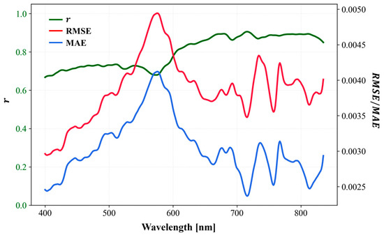
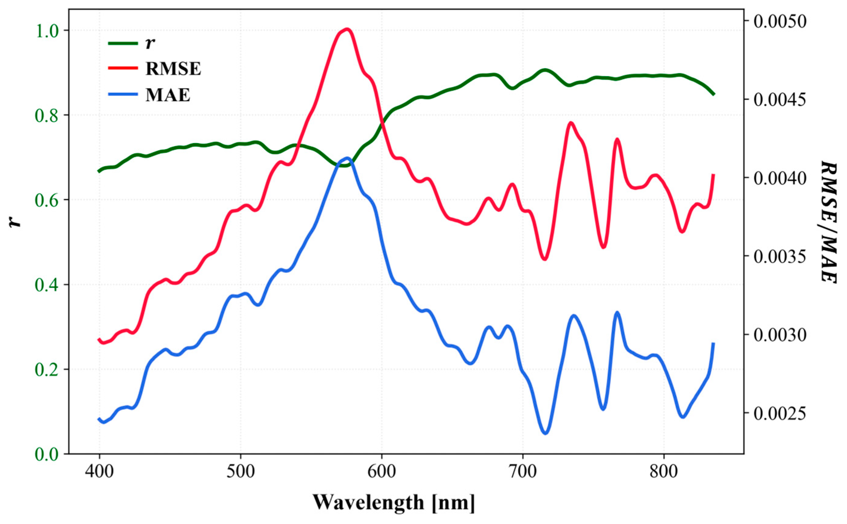
The optimal model was then applied to Sentinel-2 multispectral $R_{rs}$ to reconstruct hyperspectral $R_{rs}$ in the 400–835 nm range, and band-by-band accuracy verification was performed against in situ $R_{rs}$, the results are shown in Figure 7. It can be seen that the overall reconstruction accuracy of the model is high, with $r$ generally greater than 0.7, an average RMSE of approximately 0.0038 sr⁻¹, and an average MAE of approximately 0.0030 sr⁻¹, with significant band-specific differences. In the 400–580 nm range, $r$ generally maintained around 0.7, but RMSE and MAE increase with increasing wavelength, reaching the highest values at 580 nm (RMSE = 0.0049 sr⁻¹, MAE = 0.0041 sr⁻¹). In the 580–660 nm range, $r$ gradually increases while RMSE and MAE gradually decrease. After 660 nm, $r$ stabilizes at approximately 0.88, with slight fluctuations in RMSE and MAE (approximately 0.0039 sr⁻¹ and 0.0028 sr⁻¹, respectively).

Figure 7. Reconstruction accuracy evaluation result with in situ $R_{rs}$ of each band.

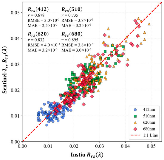
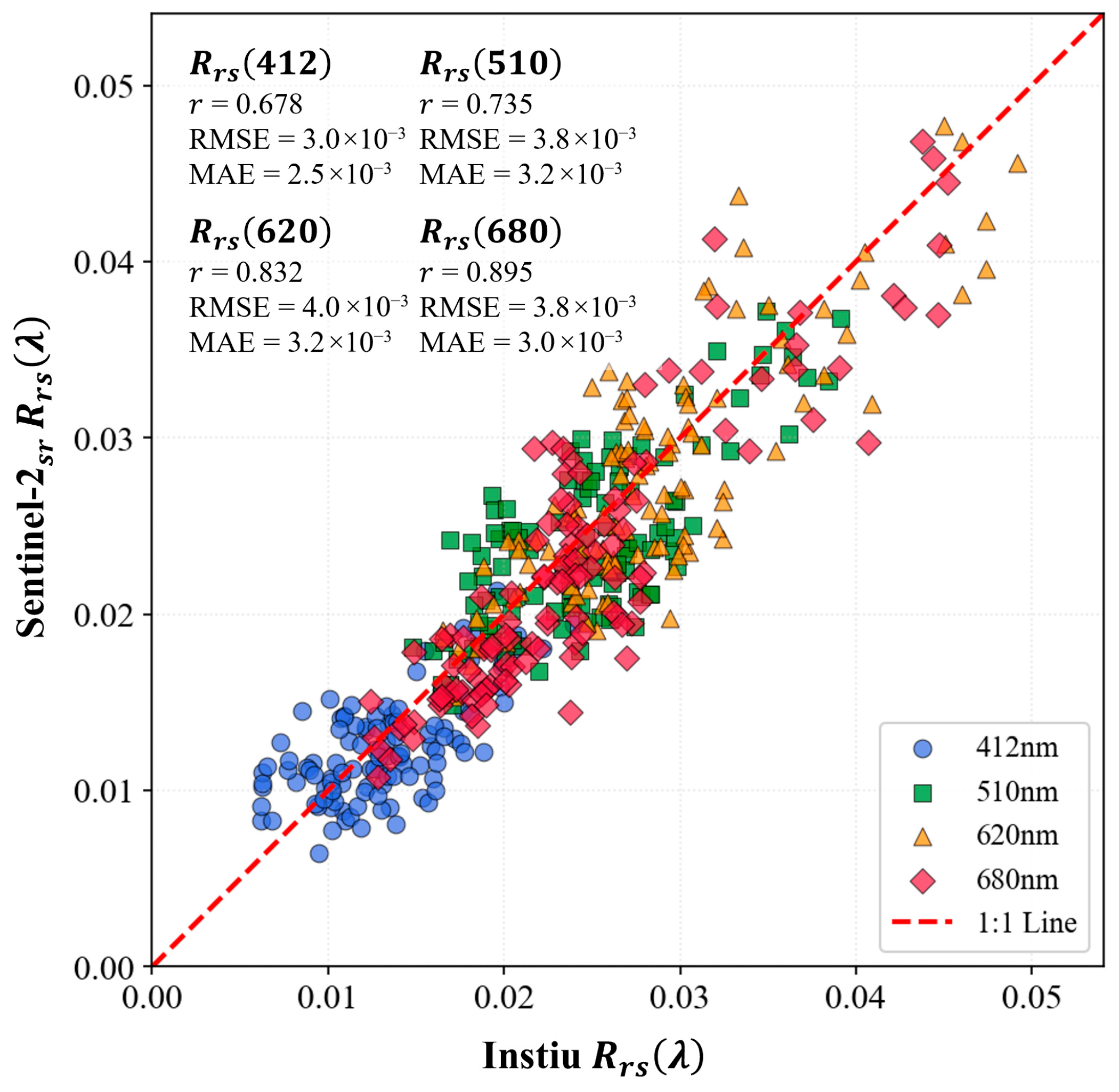
To more intuitively demonstrate the reconstruction effect, the reconstructed results of four commonly used ocean color remote sensing bands (412 nm, 510 nm, 620 nm, and 680 nm) missing from Sentinel-2 were compared with in situ data. As shown in Figure 8, the verification results of the four bands are well distributed around the 1:1 line. However, when the $R_{rs}$ is higher than 0.03, there are certain deviations at 620 nm and 680 nm. Overall, the reconstructed $R_{rs}$ achieves high accuracy in these classic ocean color remote sensing bands.

Figure 8. Accuracy evaluation with in situ $R_{rs}$ of four typical spectral bands.

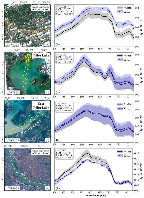
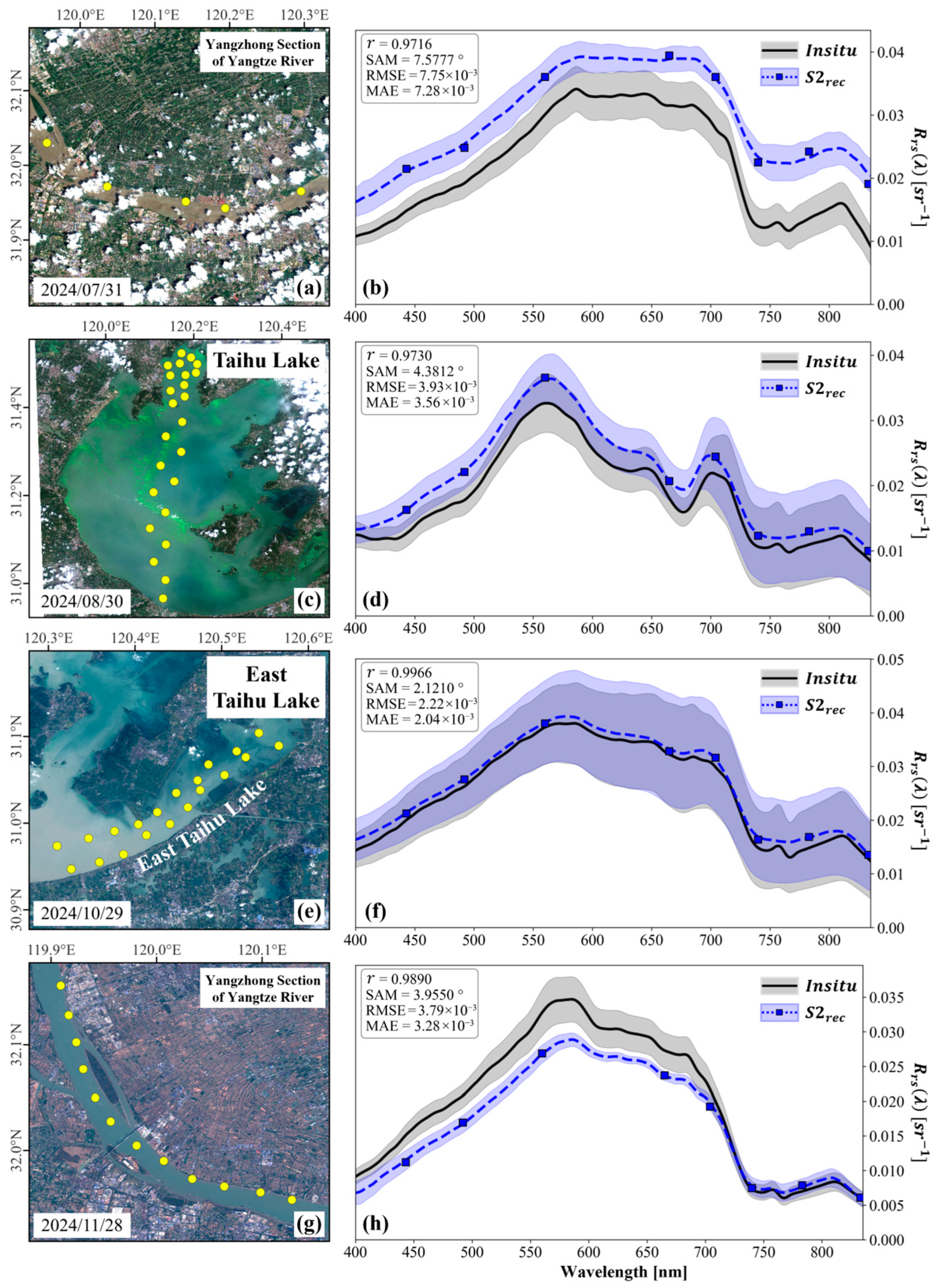
To show the reconstruction effect on different water types, $R_{rs}$ results of different water bodies from different regions and seasons were compared with the in situ $R_{rs}$. The results are shown in Figure 9. It can be seen that the $R_{rs}$ results have successfully reconstructed information that cannot be captured by the original Sentinel-2 multispectral $R_{rs}$. For example, previous studies have pointed out that as the sediment concentration increases, the $R_{rs}$ peak of water at 560 nm will gradually shift to the red band, a phenomenon known as “red shift” [62]. In Figure 9, the reconstructed spectra well restore this phenomenon: in Figure 9d (Taihu Lake algal bloom water with low sediment concentration), the reflectance peak is located at 560 nm; in Figure 9b,f,h, $R_{rs}$ in the red band increases to varying degrees with the increase in sediment concentration. For the Yangtze River water in the dry season with moderate sediment concentration (Figure 9h) and turbid Taihu Lake water (Figure 9f), the $R_{rs}$ peak shifts from 560 nm to around 580 nm; for the Yangtze River water in the flood season with high sediment concentration (Figure 9b), $R_{rs}$ is high in the 580–680 nm range. For Taihu Lake algal bloom water with high chlorophyll concentration (Figure 9d), a $R_{rs}$ shoulder is formed near 625 nm due to the absorption of phycocyanin, and a $R_{rs}$ valley is formed near 680 nm due to the strong absorption of chlorophyll a. In addition, the $R_{rs}$ peak at 820 nm caused by the backscattering of inorganic suspended solids is also well restored. However, $R_{rs}$ fluctuation characteristics caused by oxygen absorption near 760 nm were not learned, resulting in a relatively smooth reconstructed spectrum at this position. Moreover, in Taihu Lake algal bloom water (Figure 9d), $R_{rs}$ at 400 nm is relatively high due to the scattering of a large number of algal particles, which is not well restored by the reconstruction results. This may be due to the insufficient richness of the algal bloom water spectral dataset.

Figure 9. Comparison of in situ $R_{rs}$ and reconstructed $R_{rs}$ in four different water types. Yellow dots represent locations of in situ sampling points. (a,b) High sediment concentration water of the Yangtze River during its flood season. (c,d) Water of the Taihu Lake with moderate algae bloom. (e,f) Water of the Taihu Lake with high sediment concentration. (g,h) Moderate sediment concentration water of the Yangtze River during its dry season.

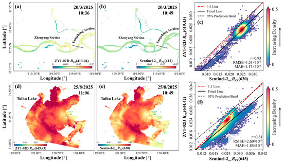
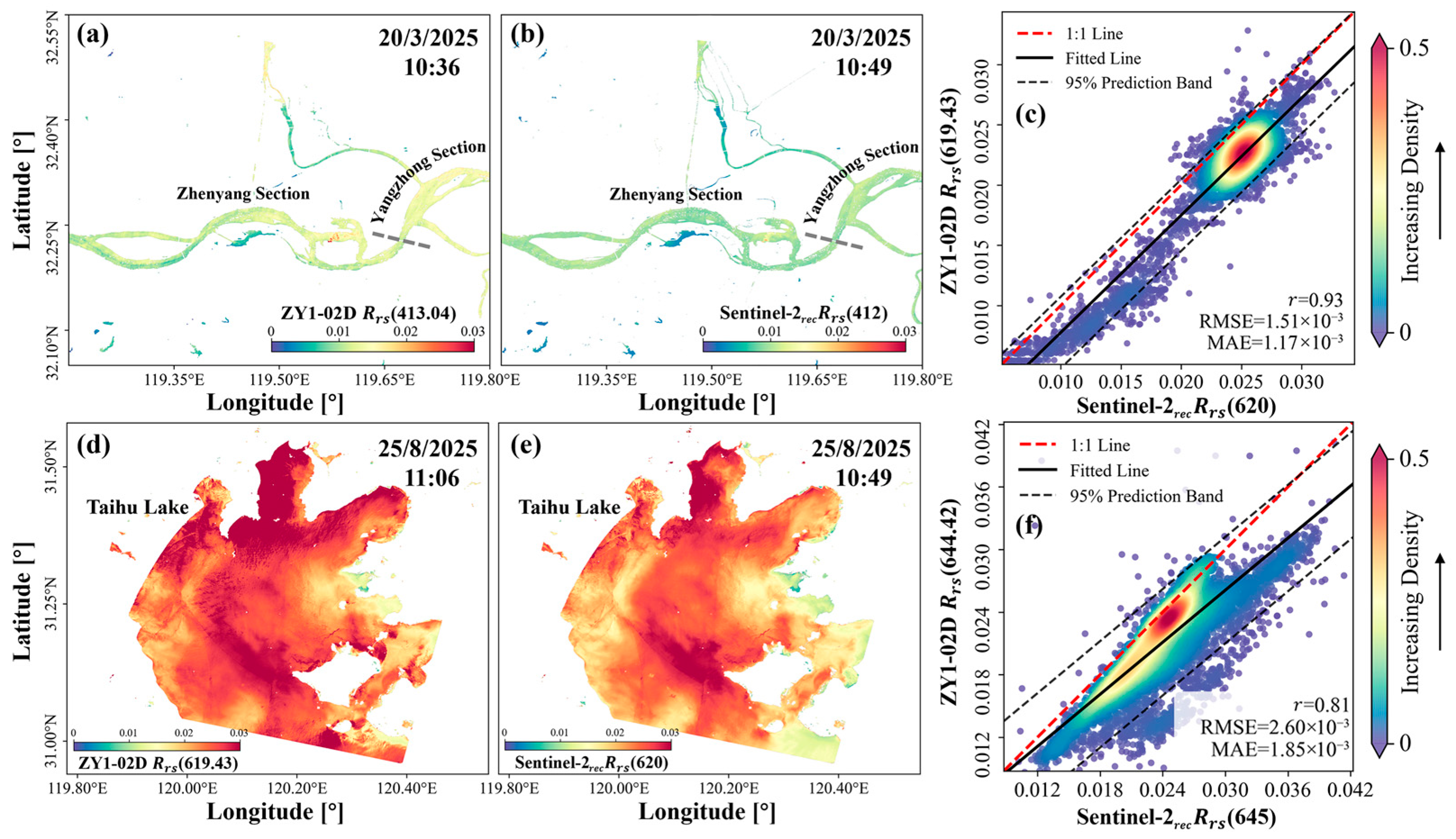
Figure 10 shows the spatial consistency comparison between the Sentinel-2 reconstructed hyperspectral $R_{rs}$ and the ZY1-02D $R_{rs}$ acquired on the same day. For the relatively turbid Yangtze River water (Figure 10a–c), the band value of the reconstructed Sentinel-2 $R_{rs}$ at 412 nm has high spatial consistency with the 413 nm (closest band to 412nm) band value of ZY1-02D. However, in the main stream of the Yangtze River, the values of ZY1-02D are generally about 0.003 sr⁻¹ higher than those of Sentinel-2. The two have a very good corresponding relationship at 620 nm, with $r$ of 0.93, RMSE of only 0.0015 sr⁻¹, and MAE of 0.0012 sr⁻¹. For Taihu Lake algal bloom water (Figure 10d–f), ZY1-02D $R_{rs}$ of 620 nm has high spatial consistency with the Sentinel-2 reconstruction results, while there are certain deviations between its 645 nm corresponding band and the Sentinel-2 reconstruction results in some water areas, with $r$ of 0.81, RMSE of 0.0026 sr⁻¹, and MAE of 0.0019 sr⁻¹. It can be seen that for characteristic bands such as 412 nm, 620 nm, and 645 nm, the reconstructed Sentinel-2 hyperspectral $R_{rs}$ not only has high accuracy, but also the spatial details it reveals are very consistent with genuine hyperspectral satellites.

Figure 10. Comparison of ZY1-02D $R_{rs}$ and reconstructed Sentinel-2 $R_{rs}$ in typical spectral bands. (a–c) example of the Yangtze River and (d–f) example of the Tai Lake.

3.5. Potential and Future Perspectives

During the model training, the hyperspectral $R_{rs}$, reconstructed by a machine learning model, well restores the true hyperspectral $R_{rs}$ information, including details such as the sediment $R_{rs}$ peak and chlorophyll absorption valley. On the test set, the average SAM between the reconstructed $R_{rs}$ and original hyperspectral $R_{rs}$ is only 1.23°, with $r$ higher than 0.99 (Figure 6). When the model is applied to Sentinel-2 images, validation with in situ measured $R_{rs}$ shows that the SAM is generally less than 5° and r is higher than 0.7 (Figure 7); further comparison between hyperspectral satellite images and reconstructed hyperspectral Sentinel-2 images on the same day also shows that reconstructed images align well with genuine hyperspectral satellite observation in spatial pattern (Figure 10). However, the reconstruction accuracy is directly affected by the atmospheric correction accuracy. For example, in Figure 9a,b, possibly due to the influence of the cloud, although the $R_{rs}$ of Sentinel-2 is well restored after reconstruction, the atmospheric correction results of Sentinel-2 on that day were generally about 0.008 sr⁻¹ higher than the in situ values, and this overall deviation is retained in the reconstructed $R_{rs}$. In a cloud-free situation (Figure 9g,h), the reconstructed $R_{rs}$ almost completely match the in situ spectra in the 700–835 nm range, but the atmospheric correction results of Sentinel-2 in the 400–700 nm range were about 0.005 sr⁻¹ lower than the in situ values, leading to lower reconstructed $R_{rs}$ than the in situ $R_{rs}$ in this band range. It can be seen that the reconstruction model in this study can only restore spectral shape information when the input multispectral $R_{rs}$ data itself contains errors, the model is unable to correct such errors. To improve the reconstruction accuracy, the accuracy of atmospheric correction for the input multispectral images must be ensured.

Regarding the input dataset, this study significantly expanded the $R_{rs}$ database based on $R_{rs}$ provided by high-quality hyperspectral satellite images, especially for the $R_{rs}$ of water types with limited in situ data, such as algal bloom water. The results show that the expansion of data volume significantly improves the model’s reconstruction effect, demonstrating that extracting water spectra from hyperspectral images for model training is a feasible approach for such studies. However, since this study only used GF-5 and ZY1-02D data from the Taihu Lake and Yangtze River Basin, the data volume is relatively scarce. To avoid information redundancy, only 6768 water spectra were extracted from the hyperspectral images. Nevertheless, by integrating data from more hyperspectral satellites (e.g., PRISMA, PACE, and Hyperion), the water spectral database can be greatly expanded, further enhancing the model’s reconstruction effect for different water types. Moreover, the resampling process during orthometric correction of hyperspectral satellite data and spatial resolution unification of Sentinel-2 MSI may introduce extra uncertainty; however, considering the high spatial homogeneity of water pixels, such uncertainty is ignored in this study.

Furthermore, to demonstrate the potential of spectral reconstruction, this study reconstructed the eight-band multispectral $R_{rs}$ of Sentinel-2 in the 400–835 nm range into 436 hyperspectral bands with 1 nm intervals, and evaluated the reconstruction accuracy of each band. However, for water color remote sensing, such a large number of bands and high spectral resolution are somewhat unnecessary, and the spectral up-sampling of GF-5 and ZY1-02D, which has a spectral resolution lower than 1 nm, may also introduce uncertainty into model training. Previous studies have pointed out that as long as the spectral bands are at appropriate wavelength positions, fewer than 20 bands can provide spectral information almost equivalent to hyperspectral measurements [59,60]. To reduce band redundancy, in subsequent model training, algorithms such as Simulated Annealing (SA) and Competitive Adaptive Reweighted Sampling (CARS) should be applied to the hyperspectral $R_{rs}$ database with reference to previous studies [63], to select bands with rich spectral features and reduce the number of output bands of the reconstruction results.

4. Conclusions

In this study, based on in situ measurements and hyperspectral satellite-derived $R_{rs}$ data, we tested the spectral reconstruction performance of six machine learning models and reconstructed the multispectral data of Sentinel-2 MSI imagery in the visible light range into hyperspectral data with a 1 nm resolution. The results demonstrate that expanding the model input dataset by cluster-sampling the hyperspectral satellite $R_{rs}$ database can effectively improve the accuracy of spectral reconstruction. Accuracy verification against in situ data shows that the reconstructed Sentinel-2 hyperspectral data achieves high precision, with the SAM generally below 5° and the $r$ higher than 0.7. The reconstructed $R_{rs}$ can well reveal spectral information that is not captured by the original Sentinel-2 data, such as the suspended sediment $R_{rs}$ peak at 580 nm and the chlorophyll absorption valley at 680 nm. Combining spectral reconstruction technology with Sentinel-2 imagery enables the acquisition of hyperspectral data with a 10 m spatial resolution and a revisit cycle of less than 5 days, which provides new perspectives for studies such as phytoplankton community identification and algal bloom extraction.

References

- Ying, Y.; Xianchuang, F.; Zhou, C.; Shihong, W.; Dongchang, L.; Gang, X.; Guangtao, L.; Liyan, G. Urban black and odorous water body mapping from Gaofen-2 images. Open Geosci. 2022, 14, 1190–1205. [Google Scholar] [CrossRef] [Scilit]
- Smith, K.; Terrano, J.; Pitchford, J.; Archer, M. Coastal Wetland Shoreline Change Monitoring: A Comparison of Shorelines from High-Resolution WorldView Satellite Imagery, Aerial Imagery, and Field Surveys. Remote Sens. 2021, 13, 3030. [Google Scholar] [CrossRef] [Scilit]
- Chen, X.; Shang, S.; Lee, Z.; Qi, L.; Yan, J.; Li, Y. High-frequency observation of floating algae from AHI on Himawari-8. Remote Sens. Environ. 2019, 227, 151–161. [Google Scholar] [CrossRef] [Scilit]
- Li, R.; Shen, F.; Zhang, Y.; Li, Z.; Chen, S. Identifying algal bloom types and analyzing their diurnal variations using GOCI-II data. Int. J. Appl. Earth Obs. Geoinf. 2025, 136, 104377. [Google Scholar] [CrossRef] [Scilit]
- Chen, S.; Shen, F.; Li, R.; Zhang, Y.; Li, Z. Deriving Coastal Sea Surface Current by Integrating a Tide Model and Hourly Ocean Color Satellite Data. Remote Sens. 2025, 17, 874. [Google Scholar] [CrossRef] [Scilit]
- Niroumand-Jadidi, M.; Bovolo, F.; Bruzzone, L. Water Quality Retrieval from PRISMA Hyperspectral Images: First Experience in a Turbid Lake and Comparison with Sentinel-2. Remote Sens. 2020, 12, 3984. [Google Scholar] [CrossRef] [Scilit]
- Kremezi, M.; Kristollari, V.; Karathanassi, V.; Topouzelis, K.; Kolokoussis, P.; Nicolo, T.; Aiello, A.; Ceriola, G.; Barbone, E.; Corradi, P. Pansharpening PRISMA Data for Marine Plastic Litter Detection Using Plastic Indexes. IEEE Access 2021, 9, 61955–61971. [Google Scholar] [CrossRef] [Scilit]
- Dierssen, H.; Bracher, A.; Brando, V.; Loisel, H.; Ruddick, K. Data Needs for Hyperspectral Detection of Algal Diversity Across the Globe. Oceanography 2020, 33, 74–79. [Google Scholar] [CrossRef] [Scilit]
- Pahlevan, N.; Smith, B.; Binding, C.; Gurlin, D.; Li, L.; Bresciani, M.; Giardino, C. Hyperspectral retrievals of phytoplankton absorption and chlorophyll-a in inland and nearshore coastal waters. Remote Sens. Environ. 2020, 253, 112200. [Google Scholar] [CrossRef] [Scilit]
- Zhang, Y.; Shen, F.; Zhao, H.; Sun, X.; Zhu, Q.; Li, M. Optical distinguishability of phytoplankton species and its implications for hyperspectral remote sensing discrimination potential. J. Sea Res. 2024, 202, 102540. [Google Scholar] [CrossRef] [Scilit]
- Zhang, Y.; Shen, F.; Li, R.; Li, M.; Li, Z.; Sun, X. Global estimation of phytoplankton functional types using PACE OCI hyperspectral data and a novel deep ensemble learning approach. Int. J. Appl. Earth Obs. Geoinf. 2026, 148, 105225. [Google Scholar] [CrossRef] [Scilit]
- Chang, P.; Lin, J.; Lin, C.; Tang, P.; Liu, Y. Optimization-Based Hyperspectral Spatiotemporal Super-Resolution. IEEE Access 2022, 10, 1. [Google Scholar] [CrossRef] [Scilit]
- Wen, Y.; Chen, P.; Zhang, Z.; Li, Y. Cross-Attention-Based High Spatial-Temporal Resolution Fusion of Sentinel-2 and Sentinel-3 Data for Ocean Water Quality Assessment. Remote Sens. 2024, 16, 4781. [Google Scholar] [CrossRef] [Scilit]
- Dong, C.; Loy, C.C.; He, K.; Tang, X. Image Super-Resolution Using Deep Convolutional Networks. IEEE Trans. Pattern Anal. Mach. Intell. 2016, 38, 295–307. [Google Scholar] [CrossRef] [Scilit]
- Yin, Z.; Ling, F.; Li, X.; Cai, X.; Chi, H.; Li, X.; Wang, L.; Zhang, Y.; Du, Y. A Cascaded Spectral-Spatial CNN Model for Super-Resolution River Mapping with MODIS Imagery. IEEE Trans. Geosci. Remote Sens. 2022, 60, 5614213. [Google Scholar] [CrossRef] [Scilit]
- Feng, G.; Jeffrey, M.; Mathew, S.; Forrest, H. On the blending of the Landsat and MODIS surface reflectance: Predicting daily Landsat surface reflectance. IEEE Trans. Geosci. Remote Sens. 2006, 44, 2207–2218. [Google Scholar] [CrossRef] [Scilit]
- Pan, Y.; Shen, F.; Wei, X. Fusion of Landsat-8/OLI and GOCI Data for Hourly Mapping of Suspended Particulate Matter at High Spatial Resolution: A Case Study in the Yangtze (Changjiang) Estuary. Remote Sens. 2018, 10, 158. [Google Scholar] [CrossRef] [Scilit]
- Shu, L.; Zhu, L.; Bak, J.; Zoogman, P.; Han, H.; Liu, S.; Li, X.; Sun, S.; Li, J.; Chen, Y.; et al. Improving ozone simulations in Asia via multisource data assimilation: Results from an observing system simulation experiment with GEMS geostationary satellite observations. Atmos. Chem. Phys. 2023, 23, 3731–3748. [Google Scholar] [CrossRef] [Scilit]
- Kislik, C.; Dronova, I.; Grantham, T.E.; Kelly, M. Mapping algal bloom dynamics in small reservoirs using Sentinel-2 imagery in Google Earth Engine. Ecol. Indic. 2022, 140, 109041. [Google Scholar] [CrossRef] [Scilit]
- Wieland, M.; Martinis, S. Large-scale surface water change observed by Sentinel-2 during the 2018 drought in Germany. Int. J. Remote Sens. 2020, 41, 4740–4754. [Google Scholar] [CrossRef] [Scilit]
- Qiao, B.; Du, T.; Ju, J.; Zhu, L. Water depth inversion based on ICESat-2 and Sentinel-2—A case study of Qiagui Co and Ayakekumu Lake on the Tibetan Plateau. J. Hydrol. Reg. Stud. 2025, 59, 102354. [Google Scholar] [CrossRef] [Scilit]
- Sent, G.; Biguino, B.; Favareto, L.; Cruz, J.; Sá, C.; Dogliotti, A.; Palma, C.; Brotas, V.; Brito, A. Deriving Water Quality Parameters Using Sentinel-2 Imagery: A Case Study in the Sado Estuary, Portugal. Remote Sens. 2021, 13, 1043. [Google Scholar] [CrossRef] [Scilit]
- Jiang, D.; Matsushita, B.; Pahlevan, N.; Gurlin, D.; Fichot, C.G.; Harringmeyer, J.; Sent, G.; Brito, A.C.; Brotas, V.; Werther, M.; et al. Estimating the concentration of total suspended solids in inland and coastal waters from Sentinel-2 MSI: A semi-analytical approach. ISPRS J. Photogramm. Remote Sens. 2023, 204, 362–377. [Google Scholar] [CrossRef] [Scilit]
- Paulino, R.S.; Martins, V.; Novo, E.; Barbosa, C.; Maciel, D.; Wanderley, R.; Portela, C.; Brocca Caballero, C.; Lima, T. Generation of robust 10-m Sentinel-2/3 synthetic aquatic reflectance bands over inland waters. Remote Sens. Environ. 2025, 318, 114593. [Google Scholar] [CrossRef] [Scilit]
- Yongchao, W.; Lee, Z.; Wei, J.; Shang, S.; Wang, M.; Lai, W. Extending satellite ocean color remote sensing to the near-blue ultraviolet bands. Remote Sens. Environ. 2021, 253, 112228. [Google Scholar]
- Young, S.; Lin, C. Spectral Super-Resolution via Adversarial Unfolding and Data-Driven Spectrum Regularization: From Multispectral Satellite Data to NASA Hyperspectral Image. arXiv 2026, arXiv:2603.00920. [Google Scholar] [CrossRef] [Scilit]
- Cai, L.; Chen, S.; Yan, X.; Bai, Y.; Bu, J. Study on High-Resolution Suspended Sediment Distribution under the Influence of Coastal Zone Engineering in the Yangtze River Mouth, China. Remote Sens. 2022, 14, 486. [Google Scholar] [CrossRef] [Scilit]
- Song, T.; Zhang, H.; Xu, Y.; Dai, X.; Fan, F.; Wang, Y.; Liu, G. Cyanobacterial blooms in Lake Taihu: Temporal trends and potential drivers. Sci. Total Environ. 2024, 942, 173684. [Google Scholar] [CrossRef] [Scilit]
- Yu, X.; Shen, Y.; Yao, X.; Li, G.; Shi, L.; Shao, W.; Hu, J.; Diao, Y. Cross-sectional observations of algal MCYST pollution and source water pollution index changes in Dianshan Lake, Shanghai. Discov. Water 2025, 5, 13. [Google Scholar] [CrossRef] [Scilit]
- Mobley, C.D. Estimation of the remote-sensing reflectance from above-surface measurements. Appl. Opt. 1999, 38, 7442–7455. [Google Scholar] [CrossRef] [Scilit]
- Luo, W.; Li, R.; Shen, F.; Liu, J. HY-1C/D CZI Image Atmospheric Correction and Quantifying Suspended Particulate Matter. Remote Sens. 2023, 15, 386. [Google Scholar] [CrossRef] [Scilit]
- Yao, H.; Li, J.; Zhou, Y.; Liu, Y.; Jiang, D.; Yin, S.; Jiang, X.; Zhang, F.; Wang, S.; Zhang, B. A novel hyperspectral index for quantifying chlorophyll-a concentration in productive waters. Remote Sens. Environ. 2025, 328, 114847. [Google Scholar] [CrossRef] [Scilit]
- Zhu, P.; Liu, Y.; Li, J. Optimization and Evaluation of Widely-Used Total Suspended Matter Concentration Retrieval Methods for ZY1-02D’s AHSI Imagery. Remote Sens. 2022, 14, 684. [Google Scholar] [CrossRef] [Scilit]
- Zhang, H.; Hu, W.; Jiao, Y. Water Quality Parameter Retrieval with GF5-AHSI Imagery for Dianchi Lake (China). Water 2024, 16, 225. [Google Scholar] [CrossRef] [Scilit]
- Feyisa, G.L.; Meilby, H.; Fensholt, R.; Proud, S.R. Automated Water Extraction Index: A new technique for surface water mapping using Landsat imagery. Remote Sens. Environ. 2014, 140, 23–35. [Google Scholar] [CrossRef] [Scilit]
- Vanhellemont, Q.; Ruddick, K. Acolite for Sentinel-2: Aquatic Applications of MSI Imagery; ESA Communications: Noordwijk, The Netherlands, 2016. [Google Scholar]
- Vanhellemont, Q. Adaptation of the dark spectrum fitting atmospheric correction for aquatic applications of the Landsat and Sentinel-2 archives. Remote Sens. Environ. 2019, 225, 175–192. [Google Scholar] [CrossRef] [Scilit]
- Vanhellemont, Q. Sensitivity analysis of the dark spectrum fitting atmospheric correction for metre- and decametre-scale satellite imagery using autonomous hyperspectral radiometry. Opt. Express 2020, 28, 29948–29965. [Google Scholar] [CrossRef] [Scilit]
- Vanhellemont, Q.; Ruddick, K. Atmospheric correction of metre-scale optical satellite data for inland and coastal water applications. Remote Sens. Environ. 2018, 216, 586–597. [Google Scholar] [CrossRef] [Scilit]
- Hu, Y.; Zhan, H.; He, Q.; Zhan, W. Assessment of Atmospheric Correction Algorithms for Landsat-8/9 Operational Land Imager over Inland and Coastal Waters. Remote Sens. 2025, 17, 3055. [Google Scholar] [CrossRef] [Scilit]
- Tian, S.; Guo, H.; Huang, J.J.; Zhu, X.; Zhang, Z. Comprehensive comparison performances of Landsat-8 atmospheric correction methods for inland and coastal waters. Geocarto Int. 2022, 37, 15302–15323. [Google Scholar] [CrossRef] [Scilit]
- Li, W.; Tang, S.; Tian, L.; Zhao, H.; Ye, H.; Zheng, W.; Liu, Y.; Sun, L. Assessing on-orbit radiometric performance of SDGSAT-1 MII for turbid water remote sensing. Remote Sens. Environ. 2025, 321, 114683. [Google Scholar] [CrossRef] [Scilit]
- Yue, L.; Zhang, L.; Peng, R.; Zeng, C.; Duan, H.; Shen, H. Understanding the Potential, Uncertainties, and Limitations of Spatiotemporal Fusion for Monitoring Chlorophyll a Concentration in Inland Eutrophic Lakes. J. Remote Sens. 2024, 4, 0209. [Google Scholar] [CrossRef] [Scilit]
- Renosh, P.R.; Doxaran, D.; Keukelaere, L.D.; Gossn, J.I. Evaluation of Atmospheric Correction Algorithms for Sentinel-2-MSI and Sentinel-3-OLCI in Highly Turbid Estuarine Waters. Remote Sens. 2020, 12, 1285. [Google Scholar] [CrossRef] [Scilit]
- Savitzky, A.; Golay, M.J.E. Smoothing and Differentiation of Data by Simplified Least Squares Procedures. Anal. Chem. 1964, 36, 1627–1639. [Google Scholar] [CrossRef] [Scilit]
- Macqueen, J. Some methods for classification and analysis of multivariate observations. Proc. Symp. Math. Statist. 1967, 1, 281–297. [Google Scholar]
- Spyrakos, E.; O’Donnell, R.; Hunter, P.D.; Miller, C.; Scott, M.; Simis, S.G.H.; Neil, C.; Barbosa, C.C.F.; Binding, C.E.; Bradt, S.; et al. Optical types of inland and coastal waters. Limnol. Oceanogr. 2018, 63, 846–870. [Google Scholar] [CrossRef] [Scilit]
- Li, S.; Song, K.; Wang, S.; Liu, G.; Wen, Z.; Shang, Y.; Lyu, L.; Chen, F.; Xu, S.; Tao, H.; et al. Quantification of chlorophyll-a in typical lakes across China using Sentinel-2 MSI imagery with machine learning algorithm. Sci. Total Environ. 2021, 778, 146271. [Google Scholar] [CrossRef] [Scilit]
- Xue, K.; Ma, R.; Wang, D.; Shen, M. Optical Classification of the Remote Sensing Reflectance and Its Application in Deriving the Specific Phytoplankton Absorption in Optically Complex Lakes. Remote Sens. 2019, 11, 184. [Google Scholar] [CrossRef] [Scilit]
- Rousseeuw, P.J. Silhouettes: A graphical aid to the interpretation and validation of cluster analysis. J. Comput. Appl. Math. 1987, 20, 53–65. [Google Scholar] [CrossRef] [Scilit]
- Breiman, L. Random Forests. Mach. Learn. 2001, 45, 5–32. [Google Scholar] [CrossRef] [Scilit]
- Geurts, P.; Ernst, D.; Wehenkel, L. Extremely randomized trees. Mach. Learn. 2006, 63, 3–42. [Google Scholar] [CrossRef] [Scilit]
- Ke, G.; Meng, Q.; Finley, T.; Wang, T.; Chen, W.; Ma, W.; Ye, Q.; Liu, T. LightGBM: A Highly Efficient Gradient Boosting Decision Tree. In Neural Information Processing Systems; Curran Associates Inc.: Red Hook, NY, USA, 2017. [Google Scholar]
- Chen, T.; Guestrin, C. XGBoost: A Scalable Tree Boosting System. In Proceedings of the 22Nd Acm Sigkdd International Conference On Knowledge Discovery and Data Mining; Association for Computing Machinery: New York, NY, USA, 2016. [Google Scholar]
- Ostroumova, L.; Gusev, G.; Vorobev, A.; Dorogush, A.V.; Gulin, A. CatBoost: Unbiased boosting with categorical features. In Neural Information Processing Systems; Curran Associates Inc.: Red Hook, NY, USA, 2017. [Google Scholar]
- Rumelhart, D.E.; Hinton, G.E.; Williams, R.J. Learning representations by back-propagating errors. Nature 1986, 323, 533–536. [Google Scholar] [CrossRef] [Scilit]
- Neagoe, I.; Faur, D.; Vaduva, C.; Datcu, M. Band Reconstruction Using a Modified UNet for Sentinel-2 Images. IEEE J. Sel. Top. Appl. Earth Observ. Remote Sens. 2023, 16, 6739–6757. [Google Scholar] [CrossRef] [Scilit]
- Wang, B.; Jia, K.; Liang, S.; Xie, X.; Wei, X.; Zhao, X.; Yao, Y.; Zhang, X. Assessment of Sentinel-2 MSI Spectral Band Reflectances for Estimating Fractional Vegetation Cover. Remote Sens. 2018, 10, 1927. [Google Scholar] [CrossRef] [Scilit]
- Lee, Z.; Shang, S.; Hu, C.; Zibordi, G. Spectral interdependence of remote-sensing reflectance and its implications on the design of ocean color satellite sensors. Appl. Opt. 2014, 53, 3301–3310. [Google Scholar] [CrossRef] [Scilit]
- Lee, Z.; Carder, K.; Arnone, R.; He, M. Determination of Primary Spectral Bands for Remote Sensing of Aquatic Environments. Sensors 2007, 7, 3428–3441. [Google Scholar] [CrossRef] [Scilit]
- Moore, T.S.; Dowell, M.D.; Bradt, S.; Ruiz Verdu, A. An optical water type framework for selecting and blending retrievals from bio-optical algorithms in lakes and coastal waters. Remote Sens. Environ. 2014, 143, 97–111. [Google Scholar] [CrossRef] [Scilit]
- Ma, R.; Jiang, G.; Duan, H.; Bracchini, L.; Loiselle, S. Effective upwelling irradiance depths in turbid waters: A spectral analysis of origins and fate. Opt. Express 2011, 19, 7127–7138. [Google Scholar] [CrossRef] [Scilit]
- Medjahed, S.A.; Ouali, M. Band selection based on optimization approach for hyperspectral image classification. Egypt. J. Remote Sens. Space Sci. 2018, 21, 413–418. [Google Scholar] [CrossRef] [Scilit]
Disclaimer/Publisher’s Note: The statements, opinions and data contained in all publications are solely those of the individual author(s) and contributor(s) and not of MDPI and/or the editor(s). MDPI and/or the editor(s) disclaim responsibility for any injury to people or property resulting from any ideas, methods, instructions or products referred to in the content. |
© 2026 by the authors. Licensee MDPI, Basel, Switzerland. This article is an open access article distributed under the terms and conditions of the Creative Commons Attribution (CC BY) license.