An Improved Multiple-Component Decomposition Method of Polarimetric SAR Interferometry Using Refined Volume Scattering Models

Highlights

What are the main findings?

• This paper employs a deorientation technique as an alternative to traditional angle compensation methods. This approach compensates for both the angle between the building and the SAR azimuth, and the angle between the building and the line of sight.
• A refined Wishart mixture model (RWMM) is proposed as a conditional branch to distinguish between building and vegetation areas. This model facilitates the effective selection of volume scattering models. Concurrently, by combining the polarimetric interferometric optimal parameter, the refined volume scattering models have been optimized, and a new multi-component decomposition method has been proposed.

What are the implications of the main findings?

• The proposed method provides a detailed explanation of the scattering mechanisms for different land cover types and mitigates the limitations caused by overestimation of volume scattering. For urban areas, particularly those with large orientation angles, this approach yields more reasonable interpretations of scattering mechanisms.

Abstract

In this research paper, we introduce an improved multiple-component decomposition technique based on the refined volume scattering models (MCSMRV) for polarimetric interferometric synthetic aperture radar (PolInSAR) system. The primary objective of this methodology is to address the issue of overestimation in volume scattering (OVS) and to clarify the mixed ambiguities associated with scattering mechanisms. Our approach incorporates an innovative inversion technique for rotation angles in urban areas, alongside the newly proposed volume scattering models. Furthermore, a refined Wishart mixture model (RWMM) is proposed for distinguishing building regions from non-building regions, which can effectively support the rational selection of volume scattering models. Additionally, the polarimetric interferometric similarity parameter (PISP) is employed to modify the volume scattering models for buildings with diverse orientation angles. To validate the effectiveness of MCSMRV, we utilize ESAR PolInSAR data and the PolInSAR data collected by the Aerospace Information Research Institute. Various mathematical methods are applied to assess the performance of MCSMRV. The experimental results clearly demonstrate that MCSMRV represents a robust method for characterizing the scattering mechanisms across different terrain types.

1. Introduction

As synthetic aperture radar (SAR) processing techniques evolve, polarimetric SAR (PolSAR) has emerged as a pivotal branch of SAR applications, providing advanced remote sensing observation capabilities for capturing polarimetric images of targets. One notable application of PolSAR is polarimetric decomposition, which serves as a crucial tool for interpreting comprehensive electromagnetic scattering information. This technique plays a fundamental role in facilitating applications such as land object classification, urban management, and ocean remote sensing, etc. [1,2,3,4,5,6,7,8,9]. The model-based approaches, as a class of PolSAR incoherent decomposition techniques, are instrumental in interpreting the scattering mechanisms of various land covers. However, model-based decomposition methods are often criticized for overestimating the volume scattering (OVS) of large oriented buildings and producing negative scattering powers. To address these limitations, researchers have developed various advanced decomposition techniques aimed at mitigating the OVS issue and significantly reducing the occurrence of negative power pixels [10,11,12,13,14,15,16,17,18,19].

The three-component decomposition method (FDD) introduced by Freeman and Durden stands out as a notable model-based approach [12]. This method decomposes the coherency matrix into a weighted sum of three scattering models. Despite its simplicity and ease of implementation, it is limited by the OVS due to its reflection symmetry assumption. Addressing this, Yamaguchi et al. incorporated the helix scattering term into FDD, resulting in the four-component decomposition method (Y4O) [13]. By accounting for the imaginary part of $T_{23}$, Y4O mitigates the volume scattering component. Building on Y4O, Yamaguchi et al. introduced orientation angle compensation (OAC) to propose a new four-component decomposition method (Y4R), which further reduces volume scattering power and compensates for rotation angles [20]. Sato et al. extended Y4R with an extended volume scattering model (S4R), yielding superior decomposition outcomes [15]. To provide a more detailed understanding of the scattering mechanisms, Zhang et al. incorporated a wire scattering element into their PolSAR image analysis framework, thereby developing a novel multiple-component scattering method (MCSM) [14]. MCSM is particularly effective for urban area analysis. Xiang et al. further refined MCSM, yielding MCSMs [21]. In 2013, Singh et al. incorporated phase angle compensation into Y4R, presenting a generalized four-component decomposition technique known as G4U, aimed at addressing the challenge of OVS in urban environments [16]. Quan et al. extended G4U using the ratio of correlation coefficient (ExG4URcc) to describe the scattering behavior of ground objects [22]. Xiang et al. introduced a novel approach that utilized the building orientation angle to define a cross-scattering component, enabling a clearer distinction between urban cross-scattering and the HV component in their analysis [23]. Dey et al. proposed the decomposition methods for full and compact PolSAR data by introducing new roll-invariant scattering-type parameters [24]. A prevalent restriction of these decomposition techniques is that they are based on the assumption that cross-polarization and co-polarization are uncorrelated, which requires setting the elements in the third column of the first row ($T_{13}$) and the third column of the second row ($T_{23}$) of the polarimetric coherency matrix to zero. Nevertheless, in practice, polarimetric data frequently contradicts this assumption, resulting in the incomplete exploitation of polarization information. The presence of oriented buildings contributes to cross-polarized HV scattering, which in turn amplifies the volume scattering power. To address the shortcomings of the reflection symmetry assumption, Singh et al. introduced a six-component decomposition approach (6SD), which takes into account oriented dipoles and compound scattering components [17]. The method effectively minimizes volume scattering in buildings with large orientation angles.

For structures positioned perpendicular to the radar’s line of sight (LOS), coherence can be directly applied to facilitate decomposition, allowing for an effective characterization of the scattering mechanism without the need for any additional compensation. In scenarios where the angle of rotation between the vertical wall of a building and the flight path is small, the OAC technique can effectively decrease cross-polarized power. However, if this angle of rotation exceeds 22.5°, the effectiveness of OAC diminishes, leading to significant cross-polarized power contributions from these oriented structures, as noted in previous studies by Chen et al. [25] and Sun et al. [26]. Chen et al. further demonstrated that, even after applying OAC compensation, a substantial volume scattering contribution persists [25]. Analogously, Deng et al. found that the volume scattering in forest canopies is not solely due to terrain slopes but also caused by randomly oriented, cylindrical scatterers [27]. The effectiveness of OAC technique is confined to a specific range of rotation angles. If the oriented angle surpasses this range, OAC may introduce notable problems, as emphasized in various studies [28,29,30,31].

To mitigate errors arising from the OAC process and address the issue of OVS, the existing decomposition methodologies can broadly be categorized into two approaches: (1) Avoiding the use of OAC and maximizing the utilization of coherency matrix elements; (2) Introducing novel angle compensation techniques specifically tailored for decomposition tasks. Singh et al. introduced a seven-component decomposition method (7SD) without requiring matrix rotation [18]. To elucidate the physical significance of the real and imaginary parts of $T_{13}$ and $T_{23}$, Wang et al. introduced two coupling scattering components, which effectively characterize these matrix elements [32]. Additionally, Li et al. devised a novel method for determining rotation angles in urban landscapes, taking into account both the angle between buildings and the SAR azimuth direction, as well as the angle between buildings and the SAR LOS [33]. This method offers a practical solution for compensating rotation angles in urban areas. Subsequently, Malik et al. proposed a nine-component decomposition approach that fully utilizes all coherency matrix elements [34].

Over the past few decades, advancements in volume scattering models and the integration of auxiliary mathematical tools have led to the development of numerous improved decomposition techniques aimed at addressing OVS and minimizing the occurrence of negative scattering powers [21,22,35,36]. Although these decomposition methods offer significant performance improvements, they often face limitations due to the computational overhead associated with additional parameters. Therefore, in this paper, we propose refined volume scattering models that efficiently describe the scattering mechanisms of different land covers. By selecting appropriate volume scattering models, we can precisely represent the scattering characteristics of various terrain types with different orientation angles, thereby clarifying the scattering mechanism and eliminating ambiguity.

In the realm of polarimetric interferometric SAR (PolInSAR) data, decomposition serves as a crucial method for interpreting the scattering mechanisms of targets [32,37,38,39]. By integrating interferometric and polarimetric measurement data, PolInSAR enhances coherence and enables the acquisition of complete target scattering responses, proving effective for target characterization [40], distinguishing oriented buildings from vegetated areas [41], landslide detection, and monitoring [42]. A significant parameter associated with the physical attributes of various targets is the polarimetric interferometric similarity parameter (PISP), which exhibits polarimetric dependence [38,39]. Notably, the PISP of forest areas tends to be lower compared to building areas that contain a higher concentration of permanent scatterers. Hence, in this research, we employed PISP to enhance the volume scattering models, with the goal of reducing the volume scattering power of large oriented buildings even further.

This paper introduces a model-based approach for multiple-component decomposition in PolInSAR, utilizing refined volume scattering models (MCSMRV). The objective of this methodology is to precisely interpret the scattering mechanisms of different land covers and address the challenge of OVS. Compared with the conventional methods, the contributions of the method proposed in this paper are as follows:

(1)

A novel technique for inversion of rotation angles is employed to replace the traditional OAC. Both the angle between building and the azimuth direction of SAR and the angle between building and the line of sight are compensated. This marks the first time that rotation angle inversion technology has been incorporated into a multi-component decomposition method, representing a significant improvement on existing methods.

(2)

A refined Wishart mixture model (RWMM) is proposed as a conditional branch to distinguish between building and vegetation areas. It can support the effective selection of the volume scattering model. This aspect differs entirely from the decision criteria of existing methods.

(3)

Refined volume scattering models are first applied to the multiple-component decomposition method, and these four volume scattering models are modified by the PISP. This represents a significant improvement upon the original volume scattering models.

To evaluate the effectiveness of MCSMRV, the performance of the proposed method is demonstrated using airborne L-band experimental SAR (ESAR) data and the airborne C-band dual antenna PolInSAR data collected by Aerospace Information Research Institute, Chinese Academy of Sciences (AIR). The proposed method is compared with the conventional methods, and the comparison shows the superiority of the method in mitigating the OVS and minimizing the negative scattering power.

2. Methodology

2.1. Deorientation Technique

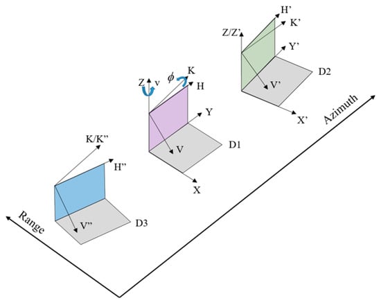
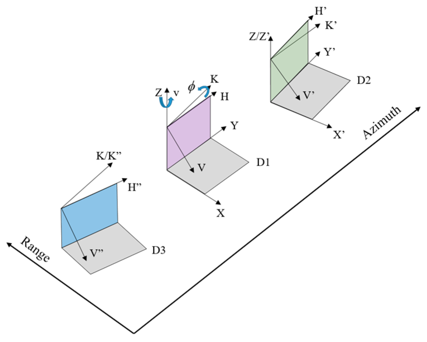
For the case of monostatic backscattering, independent and identically distributed samples were averaged to form the coherency matrix. The novel deorientation technique introduced in [33] was employed in this proposed method to rotate the coherency matrix. The schematic diagrams of parallel dihedral, rotated dihedral, and oriented dihedral are shown in Figure 1.

Figure 1. Schematic diagrams of parallel dihedral, rotated dihedral and oriented dihedral.

In Figure 1, $D_1$ represents a parallel dihedral directly facing the SAR beam direction, $D_2$ represents a rotated dihedral with an angle $\nu$ in the SAR azimuth direction, and $D_3$ represents an oriented dihedral with an angle $\varphi$ in the SAR line-of-sight direction. The $Z$ and $Z^{\prime }$ axes are perpendicular to the ground, the $K$ and $K^{″}$ axes are perpendicular to the virtual slope of $D_1$, and the $K^{\prime }$ axis is perpendicular to the virtual slope of $D_2$.

Before commencing the entire decomposition method, multi-look processing is applied to the coherency matrix to reduce noise interference, thereby obtaining the averaged coherency matrix $⟨\left[T\right]⟩$. Subsequently, the coherency matrix $⟨\left[T\right]⟩$ rotated by the novel deorientation technique is:

$$⟨\left[T^{\prime }\right]⟩=\left[R\left(\theta ,v\right)\right]⟨\left[T\right]⟩{\left[R\left(\theta ,v\right)\right]}^{\mathrm{H}}$$

(1)

where superscript ^H denotes the conjugate transpose. $\left[R\left(\theta ,v\right)\right]$ is the coherency matrix of the rotation matrix [33],

$$R\left(\theta ,v\right)=R_3{\left(\theta \right)}^{\mathrm{H}}{R}_3\left(v\right)R_3\left(\theta \right)$$

(2)

where

$$R_3\left(\theta \right)=\left[\begin{array}{ccc}\cos \theta & 0& -\sin \theta \\ 0& 1& 0\\ \sin \theta & 0& \cos \theta \end{array}\right]$$

(3)

$$R_3\left(v\right)=\left[\begin{array}{ccc}\cos v& -\sin v& 0\\ \sin v& \cos v& 0\\ 0& 0& 1\end{array}\right]$$

(4)

where $\theta$ is the incidence angle and $v$ is the rotation angle along the z-axis of the perpendicular to the horizontal ground. In this paper, an iterative solution method was employed to determine the value of $v$ that minimizes $T_{33}\left(\theta ,v\right)$. Specifically, $v$ is iterated through values within the range from −45° to 45°, with a step size of 1°, to identify the value of $v$ that yields the smallest $T_{33}\left(\theta ,v\right)$.

2.2. Refined Volume Scattering Models

Refined volume scattering models proposed in [43] were used to depict volume scattering component. Analogous to the S4R algorithm, the selection of one of the distributions (sinusoidal, cosine, or uniform scattering) was based on the ratio of co-pols.

(1)

Sinusoidal distribution

For this scenario, the probability density function (PDF) of the coherency matrix is expressed by $p\left(\theta \right)={\displaystyle \frac{1}{2}}\sin \left(\theta -{\theta }_d\right)$. The volume-averaged coherency matrix, denoted as ${⟨\left[T\right]⟩}_v^1$, can be expressed as:

$${⟨\left[T\right]⟩}_v^1=\left[\begin{array}{ccc}{\displaystyle \frac{1}{2}}& {\displaystyle \frac{\cos 2{\theta }_d}{6}}& {\displaystyle \frac{\sin 2{\theta }_d}{3}}\\ {\displaystyle \frac{\cos 2{\theta }_d}{6}}& {\displaystyle \frac{15-\cos 4{\theta }_d}{60}}& -{\displaystyle \frac{\sin 4{\theta }_d}{15}}\\ {\displaystyle \frac{\sin 2{\theta }_d}{3}}& -{\displaystyle \frac{\sin 4{\theta }_d}{15}}& {\displaystyle \frac{15+\cos 4{\theta }_d}{60}}\end{array}\right]$$

(5)

where ${\theta }_d$ represents the orientation angle, which is defined as:

$${\theta }_d={\displaystyle \frac{1}{4}}{\tan }^{-1}\left[{\displaystyle \frac{2\mathrm{Re}\left(T_{23}\right)}{T_{22}-T_{33}}}\right]$$

(6)

(2)

Cosine distribution

In this scenario, we express the PDF of the coherency matrix as $p\left(\theta \right)={\displaystyle \frac{1}{2}}\cos \left(\theta -{\theta }_d\right)$. ${⟨\left[T\right]⟩}_v^2$ can be formulated as follows:

$${⟨\left[T\right]⟩}_v^2=\left[\begin{array}{ccc}{\displaystyle \frac{1}{2}}& -{\displaystyle \frac{\cos 2{\theta }_d}{6}}& -{\displaystyle \frac{\sin 2{\theta }_d}{3}}\\ -{\displaystyle \frac{\cos 2{\theta }_d}{6}}& {\displaystyle \frac{15-\cos 4{\theta }_d}{60}}& -{\displaystyle \frac{\sin 4{\theta }_d}{15}}\\ -{\displaystyle \frac{\sin 2{\theta }_d}{3}}& -{\displaystyle \frac{\sin 4{\theta }_d}{15}}& {\displaystyle \frac{15+\cos 4{\theta }_d}{60}}\end{array}\right]$$

(7)

(3)

Uniform distribution

Analogous to S4R, the coherency matrix’s PDF is expressed by $p\left(\theta \right)={\displaystyle \frac{1}{2\pi }}$. ${⟨\left[T\right]⟩}_v^3$ can be expressed as:

$${⟨\left[T\right]⟩}_v^3={\displaystyle \frac{1}{4}}\left[\begin{array}{ccc}2& 0& 0\\ 0& 1& 0\\ 0& 0& 1\end{array}\right]$$

(8)

(4)

Volume scattering caused by oriented dihedral scatter

In urban zones, the coherency matrix’s PDF is formulated as $p\left(\theta \right)={\displaystyle \frac{1}{2}}\cos \left(\theta -{\theta }_d\right)$, and ${⟨\left[T\right]⟩}_v^4$ can be deduced as follows:

$${⟨\left[T\right]⟩}_v^4=\left[\begin{array}{ccc}0& 0& 0\\ 0& {\displaystyle \frac{15-\cos 4{\theta }_d}{30}}& 0\\ 0& 0& {\displaystyle \frac{15+\cos 4{\theta }_d}{30}}\end{array}\right]$$

(9)

2.3. Adaption of PolInSAR Volume Scattering Models

The polarimetric interferometric data from a PolInSAR system can be characterized by a $6\times 6$ coherency matrix, denoted as $⟨T_6⟩$, and defined as:

$$⟨T_6⟩=⟨\left[\begin{array}{c}{k}_m\\ k_s\end{array}\right]\left[\begin{array}{cc}{k}_m^{\mathrm{H}}& k_s^{\mathrm{H}}\end{array}\right]⟩=\left[\begin{array}{cc}⟨T_{11}⟩& ⟨{\mathrm{\Omega }}_{12}⟩\\ ⟨{\mathrm{\Omega }}_{21}⟩& ⟨T_{22}⟩\end{array}\right]$$

(10)

In the given context, the symbols $k_m$ and $k_s$ represent the scattering vectors associated with an interferometric pair. The terms $⟨T_{11}⟩$ and $⟨T_{22}⟩$ are Hermitian matrices corresponding to the master and slave polarimetric images, respectively. Furthermore, $⟨{\mathrm{\Omega }}_{12}⟩$ is a non-Hermitian matrix that encapsulates both polarimetric and interferometric data.

The polarization state significantly impacts the coherence coefficient and phase details in interferometry. By applying the theory of polarization coherence coefficients, as detailed in [44], one can project the Pauli-based scattering vectors $k_m$ and $k_s$ onto unit projection vectors ${\omega }_{\mathrm{m}}$ and ${\omega }_{\mathrm{s}}$ to obtain the PISP. The optimal PISP parameter is derived from [39]:

$$\mathrm{PISP}={\displaystyle \frac{{\left|\mathrm{Tr}\left({\omega }_m^{\mathrm{H}}{\mathrm{\Omega }}_{12}{\omega }_s\right)\right|}^2}{\mathrm{Tr}\left({\omega }_m^{\mathrm{H}}{T}_{11}{\omega }_m\right)\mathrm{Tr}\left({\omega }_s^{\mathrm{H}}{T}_{22}{\omega }_s\right)}}$$

(11)

where $\mathrm{Tr}\left(\cdot \right)$ denotes the trace of a matrix. The optimized scattering matrices for the master and slave images are represented by $\left[{\omega }_m\right]=\left[{\omega }_{m,\mathrm{opt}1},{\omega }_{m,\mathrm{opt}2},{\omega }_{m,\mathrm{opt}3}\right]$ and $\left[{\omega }_s\right]=\left[{\omega }_{s,\mathrm{opt}1},{\omega }_{s,\mathrm{opt}2},{\omega }_{s,\mathrm{opt}3}\right]$, respectively. The eigenvectors ${\omega }_{m,optj}$ and ${\omega }_{s,optj}$ ($j=1,2,3$) are mutually orthogonal, indicating that the scattering mechanisms are statistically independent.

As per [39], the PISP is unaffected by the absolute amplitude of the scattering matrix or the target’s orientation angle. Instead, PISP is a second-order statistical parameter that adeptly captures the characteristics of ground scattering and is a tool for assessing the stability of polarization interference in various terrains. Higher target stability corresponds to a larger PISP value. Since buildings exhibit deterministic scattering, whereas forests display stochastic scattering, PISP values tend to be higher in urban areas and lower in vegetation regions. This paper leveraged this statistical property to apply PISP toward minimizing the $T_{33}$ component of the volume scattering matrices, thereby effectively mitigating the impact of volume scattering in buildings with significant orientation angles.

$${⟨\left[T\right]⟩}_{v\_new}=\left[\begin{array}{ccc}{T}_{v11}& T_{v12}& T_{v13}\\ T_{v21}& T_{v22}& T_{v23}\\ T_{v31}& T_{v32}& rr{T}_{v33}\end{array}\right]$$

(12)

where $rr$ is defined as ${\displaystyle \frac{PISP}{\left(1-PISP\right)}}$, and $T_{vij}$ (with $i,j=1,2,3$) represents the elements of the coherency matrix associated with volume scattering. It should be noted that, when $PISP=1$, $rr$ should be set to 1 to avoid a mathematical logic flaw in the calculation of $rr$. As PISP rises, the $rr$ value increases, enabling flexible adjustments to the volume scattering model. When $rr$ is less than or equal to 1, the scattering mechanism in the area exhibits stochastic behavior, consistent with the volume scattering models described in [43]. However, when $rr$ exceeds 1, the scattering mechanism shifts to a deterministic nature.

2.4. Refined Multiple-Component Decomposition Method of PolInSAR

The approach introduced in this paper builds upon the multi-component decomposition technique outlined in [14], offering a valuable addition to the realm of PolInSAR decomposition methods. After the novel angle compensation, the proposed method divides the coherency matrix $⟨\left[T^{\prime }\right]⟩$ into five components: surface, volume, double-bounce, helix, and wire scattering:

$$\begin{array}{l}⟨\left[T^{\prime }\right]⟩=\left[\begin{array}{ccc}{T^{\prime }}_{11}& {T^{\prime }}_{12}& {T^{\prime }}_{13}\\ {T^{\prime }}_{12}^{\ast }& {T^{\prime }}_{22}& {T^{\prime }}_{23}\\ {T^{\prime }}_{13}^{\ast }& {T^{\prime }}_{23}^{\ast }& {T^{\prime }}_{33}\end{array}\right]=f_s⟨{\left[T^{\prime }\right]}_s⟩+f_d⟨{\left[T^{\prime }\right]}_d⟩+f_c⟨{\left[T^{\prime }\right]}_c⟩+f_w⟨{\left[T^{\prime }\right]}_w⟩+f_{vi}⟨{\left[T^{\prime }\right]}_{v\_newi}⟩\left(i=1,2,3,4\right)\\ ={\displaystyle \frac{f_s}{1+{\left|\beta \right|}^2}}\left[\begin{array}{ccc}1& {\beta }^{*}& 0\\ \beta & {\left|\beta \right|}^2& 0\\ 0& 0& 0\end{array}\right]+{\displaystyle \frac{f_d}{1+{\left|\alpha \right|}^2}}\left[\begin{array}{ccc}{\left|\alpha \right|}^2& \alpha & 0\\ {\alpha }^{*}& 1& 0\\ 0& 0& 0\end{array}\right]+{\displaystyle \frac{f_c}{2}}\left[\begin{array}{ccc}0& 0& 0\\ 0& 1& \pm j\\ 0& \mp j& 1\end{array}\right]\\ +{\displaystyle \frac{f_w}{2}}\left[\begin{array}{ccc}{\left|\gamma \right|}^2+{\gamma }^{\ast }+\gamma +1& {\left|\gamma \right|}^2+{\gamma }^{\ast }-\gamma -1& 2{\rho }^{\ast }\left(\gamma +1\right)\\ {\left|\gamma \right|}^2-{\gamma }^{\ast }+\gamma -1& {\left|\gamma \right|}^2-{\gamma }^{\ast }-\gamma +1& 2{\rho }^{\ast }\left(\gamma -1\right)\\ 2\rho \left({\gamma }^{\ast }+1\right)& 2\rho \left({\gamma }^{\ast }-1\right)& 4{\left|\rho \right|}^2\end{array}\right]+f_{vi}⟨{\left[T^{\prime }\right]}_{v\_newi}⟩,\left(i=1,2,3,4\right)\end{array}$$

(13)

where $f_s$, $f_v$, $f_d$, $f_c$, and $f_w$ are the coefficients of the coherency matrices for surface scattering, volume scattering, double-bounce scattering, helix scattering, and wire scattering, respectively. $⟨{\left[T^{\prime }\right]}_s⟩$, $⟨{\left[T^{\prime }\right]}_d⟩$, $⟨{\left[T^{\prime }\right]}_c⟩$, $⟨{\left[T^{\prime }\right]}_w⟩$, and $⟨{\left[T^{\prime }\right]}_{v\_newi}⟩$ correspond to the surface scattering, double-bounce scattering, helix scattering, wire scattering, and volume scattering coherency matrices after the novel angle compensation, respectively. $\rho$ and $\gamma$ are the ratios of the $HV$ and $HH$ backscatters to the $VV$ backscatter, respectively. $\alpha$ and $\beta$ are the shape parameters of double-bounce and surface scattering, respectively. Moreover, the volume scattering component can be obtained by selecting appropriate volume scattering models. We illustrated this process using a volume scattering model based on the sinusoidal distribution. Through mathematical manipulations, we can rearrange the relationships among the elements of $⟨\left[T^{\prime }\right]⟩$:

$$\begin{array}{l}{T^{\prime }}_{11}+{T^{\prime }}_{33}=f_s+{\left|\alpha \right|}^2{f}_d+\left({\displaystyle \frac{1}{2}}+{\displaystyle \frac{15+\cos 4{\theta }_d}{60}}rr\right)f_v+{\displaystyle \frac{1}{2}}{f}_c+\left[{\displaystyle \frac{1}{2}}\left({\left|\gamma \right|}^2+{\gamma }^{*}+\gamma +1\right)+2{\left|\rho \right|}^2\right]f_w\\ {T^{\prime }}_{11}-{T^{\prime }}_{33}=f_s+{\left|\alpha \right|}^2{f}_d+\left({\displaystyle \frac{15-\cos 4{\theta }_d}{60}}rr\right)f_v-{\displaystyle \frac{1}{2}}{f}_c+{\displaystyle \frac{1}{2}}\left({\left|\gamma \right|}^2+{\gamma }^{*}+\gamma +1-4{\left|\rho \right|}^2\right)f_w\\ {T^{\prime }}_{12}={\beta }^{*}{f}_s+\alpha f_d+{\displaystyle \frac{\cos 2{\theta }_d}{6}}{f}_v+{\displaystyle \frac{1}{2}}{f}_w\left({\left|\gamma \right|}^2+{\gamma }^{*}-\gamma -1\right)\\ {T^{\prime }}_{22}={\left|\beta \right|}^2{f}_s+f_d+{\displaystyle \frac{15-\cos 4{\theta }_d}{60}}{f}_v+{\displaystyle \frac{1}{2}}{f}_w\left({\left|\gamma \right|}^2-{\gamma }^{*}-\gamma +1\right)\end{array}$$

(14)

Using the innovative method, it is possible to deduce wire scattering and helix scattering:

$$\begin{array}{l}{f}_w={\displaystyle \frac{{T^{\prime }}_{13}}{\left[{\rho }^{*}\left(\gamma +1\right)\right]}}\\ f_c=2\left|\mathrm{Im}\left[{T^{\prime }}_{23}-f_w{\rho }^{*}\left(\gamma -1\right)\right]\right|\end{array}$$

(15)

The volume scattering component can be obtained as follows [43]:

(1)

Sinusoidal distribution:

$$P_{v1}={\displaystyle \frac{45-\cos 4{\theta }_d+rr\left(15+\cos 4{\theta }_d\right)}{2rr\left(15+\cos 4{\theta }_d\right)}}\left(2{T^{\prime }}_{33}-f_c-4{\left|\rho \right|}^2\left|f_w\right|\right)$$

(16)

(2)

Uniform distribution:

$$P_{v2}={\displaystyle \frac{3+rr}{2rr}}\left(2{T^{\prime }}_{33}-f_c-4{\left|\rho \right|}^2\left|f_w\right|\right)$$

(17)

(3)

Cosine distribution:

$$P_{v3}={\displaystyle \frac{45-\cos 4{\theta }_d+rr\left(15+\cos 4{\theta }_d\right)}{2rr\left(15+\cos 4{\theta }_d\right)}}\left(2{T^{\prime }}_{33}-f_c-4{\left|\rho \right|}^2\left|f_w\right|\right)$$

(18)

(4)

Extended volume scattering:

$$P_{v4}={\displaystyle \frac{15-\cos 4{\theta }_d+rr\left(15+\cos 4{\theta }_d\right)}{2rr\left(15+\cos 4{\theta }_d\right)}}\left(2{T^{\prime }}_{33}-f_c-4{\left|\rho \right|}^2\left|f_w\right|\right)$$

(19)

Following mathematical manipulations, we derived three equations with four variables ($\alpha$, $\beta$, $f_s$, $f_d$):

(1)

Sinusoidal distribution:

$$\begin{array}{l}S=f_s+{\left|\alpha \right|}^2{f}_d={T^{\prime }}_{11}+{T^{\prime }}_{33}-{\displaystyle \frac{f_c}{2}}-{\displaystyle \frac{\left({\left|\gamma \right|}^2+{\gamma }^{*}+\gamma +1+4{\left|\rho \right|}^2\right)f_w}{2}}-{\displaystyle \frac{\left[rr\left(15+\cos 4{\theta }_d\right)+30\right]f_{v1}}{60}}\\ D={\left|\beta \right|}^2{f}_s+f_d={T^{\prime }}_{22}-{\displaystyle \frac{f_c}{2}}-{\displaystyle \frac{\left({\left|\gamma \right|}^2-{\gamma }^{*}-\gamma +1\right)f_w}{2}}-{\displaystyle \frac{\left(15-\cos 4{\theta }_d\right)f_{v1}}{60}}\\ C=f_s{\beta }^{*}+\alpha f_d={T^{\prime }}_{12}-{\displaystyle \frac{f_v\cos 2{\theta }_d}{6}}-{\displaystyle \frac{\left({\left|\gamma \right|}^2+{\gamma }^{*}-\gamma -1\right)f_w}{2}}\end{array}$$

(20)

(2)

Uniform distribution:

$$\begin{array}{l}S=f_s+{\left|\alpha \right|}^2{f}_d={T^{\prime }}_{11}+{T^{\prime }}_{33}-{\displaystyle \frac{f_c}{2}}-{\displaystyle \frac{\left(2+rr\right)}{4}}{f}_{v2}-{\displaystyle \frac{\left({\left|\gamma \right|}^2+{\gamma }^{*}+\gamma +1+4{\left|\rho \right|}^2\right)f_w}{2}}\\ D={\left|\beta \right|}^2{f}_s+f_d={T^{\prime }}_{22}-{\displaystyle \frac{\left({\left|\gamma \right|}^2-{\gamma }^{*}-\gamma +1\right)f_w}{2}}-{\displaystyle \frac{1}{2}}{f}_c-{\displaystyle \frac{1}{2}}{f}_{v2}\\ C=f_s{\beta }^{*}+\alpha f_d={T^{\prime }}_{12}-{\displaystyle \frac{\left({\left|\gamma \right|}^2+{\gamma }^{*}-\gamma -1\right)f_w}{2}}\end{array}$$

(21)

(3)

Cosine distribution:

$$\begin{array}{l}S=f_s+{\left|\alpha \right|}^2{f}_d={T^{\prime }}_{11}+{T^{\prime }}_{33}-{\displaystyle \frac{f_c}{2}}-{\displaystyle \frac{\left({\left|\gamma \right|}^2+{\gamma }^{*}+\gamma +1+4{\left|\rho \right|}^2\right)f_w}{2}}-{\displaystyle \frac{\left[rr\left(15+\cos 4{\theta }_d\right)+30\right]f_{v3}}{60}}\\ D={\left|\beta \right|}^2{f}_s+f_d={T^{\prime }}_{22}-{\displaystyle \frac{f_c}{2}}-{\displaystyle \frac{\left({\left|\gamma \right|}^2-{\gamma }^{*}-\gamma +1\right)f_w}{2}}-{\displaystyle \frac{\left(15-\cos 4{\theta }_d\right)f_{v3}}{60}}\\ C=f_s{\beta }^{*}+\alpha f_d={T^{\prime }}_{12}+{\displaystyle \frac{f_v\cos 2{\theta }_d}{6}}-{\displaystyle \frac{\left({\left|\gamma \right|}^2+{\gamma }^{*}-\gamma -1\right)f_w}{2}}\end{array}$$

(22)

(4)

Extended volume scattering:

$$\begin{array}{l}S=f_s+{\left|\alpha \right|}^2{f}_d={T^{\prime }}_{11}+{T^{\prime }}_{33}-{\displaystyle \frac{f_c}{2}}-{\displaystyle \frac{\left({\left|\gamma \right|}^2+{\gamma }^{*}+\gamma +1+4{\left|\rho \right|}^2\right)f_w}{2}}-{\displaystyle \frac{rr\left(15+\cos 4{\theta }_d\right)}{30}}{f}_{v4}\\ D={\left|\beta \right|}^2{f}_s+f_d={T^{\prime }}_{22}-{\displaystyle \frac{f_c}{2}}-{\displaystyle \frac{\left({\left|\gamma \right|}^2-{\gamma }^{*}-\gamma +1\right)f_w}{2}}-{\displaystyle \frac{\left(15-\cos 4{\theta }_d\right)f_{v4}}{30}}\\ C=f_s{\beta }^{*}+\alpha f_d={T^{\prime }}_{12}-{\displaystyle \frac{\left({\left|\gamma \right|}^2+{\gamma }^{*}-\gamma -1\right)f_w}{2}}\end{array}$$

(23)

The leftover constants can be ascertained as follows:

When ${T^{\prime }}_{11}-{T^{\prime }}_{22}-{T^{\prime }}_{33}+P_c>0$

$$f_s=S,{\beta }^{*}={\displaystyle \frac{C}{S}},f_d=D-{\displaystyle \frac{{\left|C\right|}^2}{S}}$$

(24)

when ${T^{\prime }}_{11}-{T^{\prime }}_{22}-{T^{\prime }}_{33}+P_c\le 0$

$$f_d=D,\alpha ={\displaystyle \frac{C}{D}},f_s=S-{\displaystyle \frac{{\left|C\right|}^2}{D}}$$

(25)

The estimated scattering intensities, denoted as $P_s$ for surface scattering, $P_v$ for volume scattering, $P_d$ for double-bounce scattering, $P_c$ for helix scattering, and $P_w$ for wire scattering contributions, are as follows:

$$P_d=f_d\left(1+{\left|\alpha \right|}^2\right),P_s=f_s\left(1+{\left|\beta \right|}^2\right),P_c=f_c,P_w=f_w\left(1+{\left|\gamma \right|}^2+2{\left|\rho \right|}^2\right),P_v=f_{vi}\left(i=1,2,3,4\right)$$

(26)

In this decomposition method, the key to solving for the individual scattering components lies in utilizing the corresponding elements of the matrix to solve a system of equations for the values of the scattering components and parameters. It should be noted that, during the solution process, as the number of equations is fewer than the number of unknowns, assumptions must be made; this is a common approach in target decomposition algorithms.

2.5. Branch Condition

Branch condition for the selection of volume scattering models is an important factor that affects the accuracy of the final decomposition results. In this subsection, the RWMM is proposed to distinguish between built-up and non-built-up areas and to select the volume scattering model properly. It should be noted that all coherency matrices and related parameters used in this subsection are derived from the 6 × 6 PolInSAR coherence matrix. The main steps are as follows:

(1)

Training sample selection and initialization. According to the actual requirements, the training set of D training samples is selected, denoted as $\left\{Z_1,\dots ,Z_D\right\}$. The number of mixture components K is specified, and then K training samples from the training set are randomly selected as the class clustering center ${\mathrm{\Sigma }}_k^{\left(0\right)}$, and the superscript number indicates the number of former. The weight coefficients $\pi$ and equivalent look L are initialized as follows:

$$\begin{array}{l}{\pi }_1^{\left(0\right)}={\pi }_2^{\left(0\right)}=\dots ={\pi }_K^{\left(0\right)}={\displaystyle \frac{1}{K}}\\ L_1^{\left(0\right)}=L_2^{\left(0\right)}=\dots =L_K^{\left(0\right)}=n\end{array}$$

(27)

where n is the nominal look.

(2)

Calculation of similarity parameters. The similarity coefficient between the training sample $Z_d$ and the $k^{th}$ class clustering center is calculated as:

$${\gamma }_{kd}^{\left(i\right)}={\displaystyle \frac{{\pi }^{\left(i-1\right)}P\left(Z_d\left|L_k^{\left(i-1\right)},{\mathrm{\Sigma }}_k^{\left(i-1\right)}\right.\right)}{{\displaystyle \sum _{k=1}^{K}P\left(Z_d\left|L_k^{\left(i-1\right)},{\mathrm{\Sigma }}_k^{\left(i-1\right)}\right.\right)}}}$$

(28)

where $P\left(\cdot \right)$ is the probability density function of the complex Wishart distribution.

(3)

Parameter updates. Update the weight coefficients ${\pi }_k^{\left(i\right)}$ and the class clustering center ${\mathrm{\Sigma }}_k^{\left(i\right)}$:

$${\pi }_k^{\left(i\right)}={\displaystyle \frac{1}{D}}{\displaystyle \sum _{d=1}^D{\gamma }_{kd}^{\left(i\right)}},{\mathrm{\Sigma }}_k^{\left(i\right)}={\displaystyle \frac{{\displaystyle \sum _{d=1}^D{\gamma }_{kd}^{\left(i\right)}{Z}_d}}{{\displaystyle \sum _{d=1}^D{\gamma }_{kd}^{\left(i\right)}}}}$$

(29)

The expectation of the maximized log-likelihood function is used to determine the equivalent look $L_k^{\left(i\right)}$:

$$L_k^{\left(i\right)}=\underset{L_k^{\left(i\right)}}{\arg \max }{\displaystyle \sum _{d=1}^D{\gamma }_{kd}^{\left(i\right)}}\ln {\displaystyle \frac{{\pi }_k^{\left(i\right)}\cdot P\left(Z_d\left|L_k^{\left(i\right)},{\mathrm{\Sigma }}_k^{\left(i\right)}\right.\right)}{{\gamma }_{kd}^{\left(i\right)}}}$$

(30)

Let the first order derivative of $L_k^{\left(i\right)}$ be zero:

$$q\ln L_k^{\left(i\right)}-{\phi }_q^{\nu }\left(L_k^{\left(i\right)}\right)=\ln \left|{\mathrm{\Sigma }}_k^{\left(i\right)}\right|-q+{\displaystyle \frac{{\displaystyle \sum _{d=1}^D{\gamma }_{kd}^{\left(i\right)}\left(Tr\left(inv\left({\mathrm{\Sigma }}_k^{\left(i\right)}\right)\cdot Z_d\right)-\ln \left|Z_d\right|\right)}}{{\displaystyle \sum _{d=1}^D{\gamma }_{kd}^{\left(i\right)}}}}$$

(31)

where $inv\left(\cdot \right)$ denotes the matrix inverse and ${\phi }_q^{\nu }\left(\cdot \right)$ denotes the $v$-order multivariate Gamma function. The weight coefficients ${\pi }_k^{\left(i\right)}$ and the class clustering centers ${\mathrm{\Sigma }}_k^{\left(i\right)}$ should be treated as constants. It can be seen that the analytical expression for $L_k^{\left(i\right)}$ is difficult to obtain by derivation. Notice that the right-hand side of Equation (31) is independent of $L_k^{\left(i\right)}$ and can be viewed as a constant. The left-hand side of Equation (31) can be viewed as a function of $L_k^{\left(i\right)}$:

$$F\left(L_k^{\left(i\right)}\right)=q\ln L_k^{\left(i\right)}-{\phi }_q^{\nu }\left(L_k^{\left(i\right)}\right)$$

(32)

The first order derivative of $L_k^{\left(i\right)}$ can be obtained:

$$F^{\prime }\left(L_k^{\left(i\right)}\right)={\displaystyle \frac{q}{L_k^{\left(i\right)}}}-{\phi }_q^{\nu +1}\left(L_k^{\left(i\right)}\right)$$

(33)

For PolInSAR data satisfying reciprocity, $q=6$, $v=0$. Although it is difficult to obtain an analytical solution for $L_k^{\left(i\right)}$, the bisection method can be used to find a unique approximate solution to complete the parameter update.

Repeat Steps (2) and (3) until the weight coefficients ${\pi }_k^{\left(i\right)}$, class clustering centers ${\mathrm{\Sigma }}_k^{\left(i\right)}$, and equivalent look $L_k^{\left(i\right)}$ parameters converge. The iteration termination conditions are as follows:

$$\begin{array}{c}\left|{\pi }_k^{\left(i\right)}-{\pi }_k^{\left(i-1\right)}\right|<{\delta }_{\pi }\\ {\displaystyle \frac{1}{2}}Tr\left({\mathrm{\Sigma }}_k^{\left(i\right)}\cdot inv\left({\mathrm{\Sigma }}_k^{\left(i-1\right)}\right)+{\mathrm{\Sigma }}_k^{\left(i-1\right)}\cdot inv\left({\mathrm{\Sigma }}_k^{\left(i\right)}\right)\right)-q<{\delta }_{\mathrm{\Sigma }}\\ \left|L_k^{\left(i\right)}-L_k^{\left(i-1\right)}\right|<{\delta }_L\end{array}$$

(34)

where the left-hand side of Equation (34) is the symmetric LogDet dispersion based on the Hermitian positive definite matrix [45]. ${\delta }_{\pi }$, ${\delta }_{\mathrm{\Sigma }}$, and ${\delta }_L$ are the weight coefficients, class clustering center, and equivalent look predefined thresholds. In the text, ${\delta }_{\pi }$ and ${\delta }_{\mathrm{\Sigma }}$ were set to ${10}^{-3}$ and ${\delta }_L$ was set to ${10}^{-1}$.

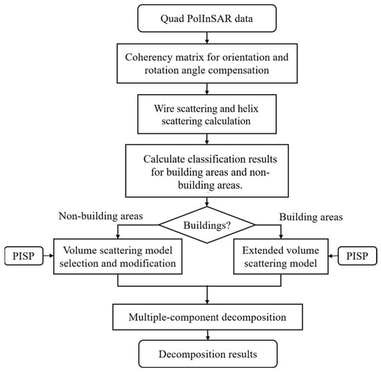
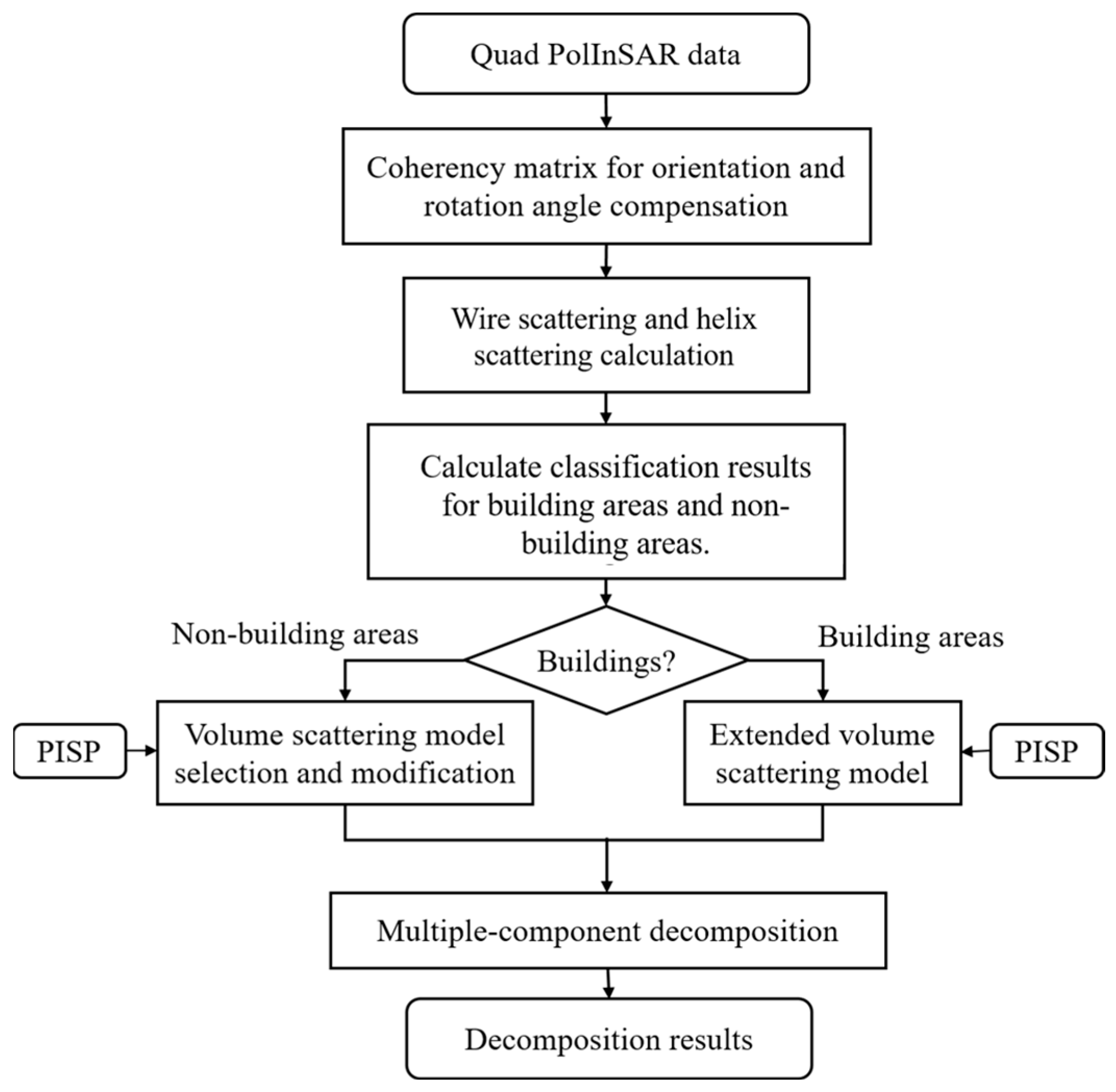
This paper outlines the processing approach of the proposed method, with its flowchart depicted in Figure 2. For values of $rr$ ranging from 0 to less than 1, $rr$ is directly employed to compute the volume scattering power. However, when $rr$ is 1 or greater, the volume scattering power remains constant, unaffected by the value of $rr$. It should be noted that all decomposition processing and parameter calculations described in this paper were based on the coherency matrix. After performing angle compensation and filtering on the coherency matrix, the parameter values and scattering power were then computed.

Figure 2. Flowchart of the proposed multi-component decomposition method.

3. Results and Discussion

3.1. ESAR PolInSAR Data

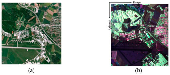
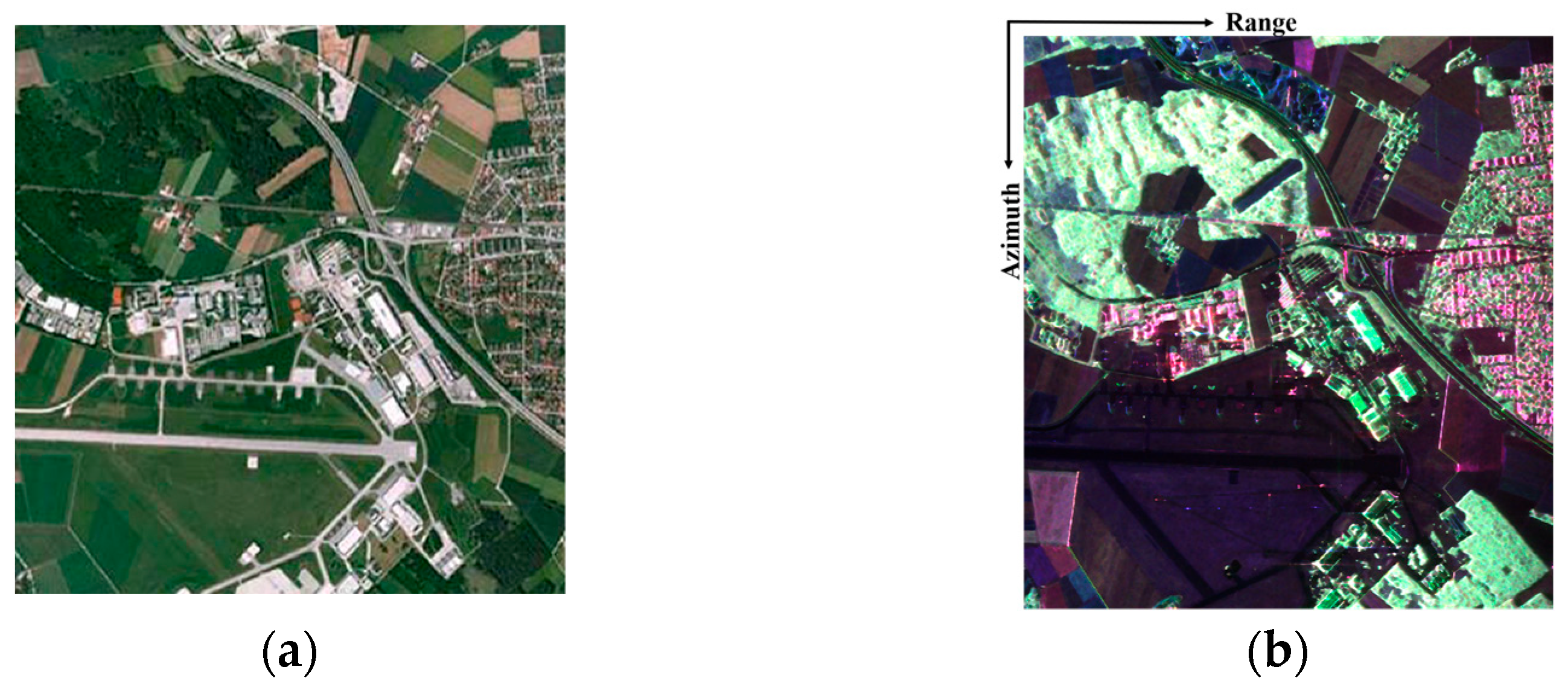
In the present research, we utilized L-band ESAR PolInSAR data to validate the efficacy of MCSMRV. Our study area, spanning 1300 by 1200 pixels, is situated in Oberpfaffenhofen, Germany. The data was acquired on 26 August 2002. The spatial resolution was 3 m × 2.2 m and the wavelength was 23 cm. This region encompasses a diverse array of landscapes, including structures with varying orientations, agricultural lands, woodland areas, and airports, among others. The temporal baseline for the imagery was confined to a single day, with an incidence angle approximating 40 degrees. The central geographical coordinates of the image are positioned at ${48}^{°}{5}^{\prime }{3}^{″}\mathrm{N}$, ${11}^{°}17^{\prime }{4}^{″}\mathrm{E}$. Figure 3 illustrates both the optical image of the study area and its corresponding color-coded Pauli representation.

Figure 3. The study region, located in Oberpfaffenhofen, Germany, was imaged using SAR technology with an E-SAR system operating in the L-band. (a) Displays a visual image sourced from Google Earth. (b) Pauli decomposition results (red: T₂₂ term; green: T₃₃ term; and blue: T₁₁ term).

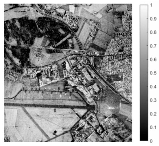
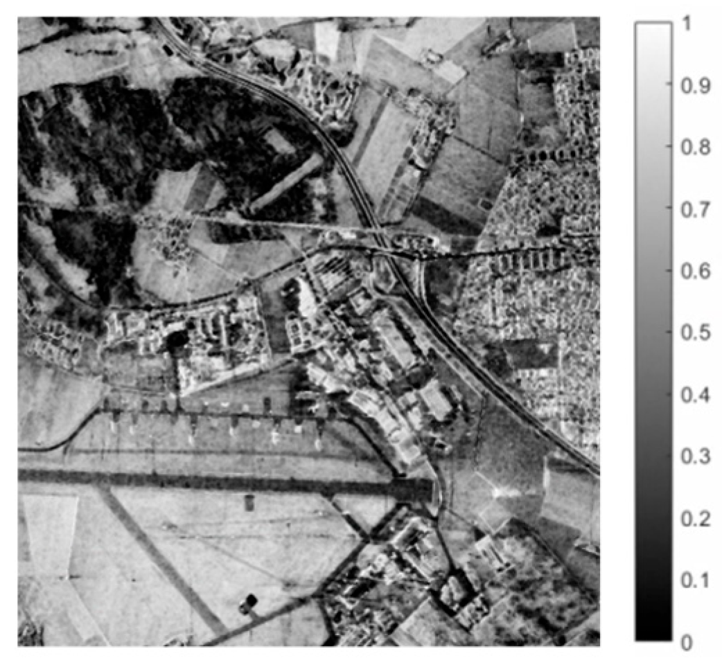
The images presented in Figure 4 depict the PISP image. From these illustrations, it is evident that the PISP has the capability to distinguish between regions exhibiting comparable scattering properties, including buildings with diverse orientation angles and vegetated areas. When the PISP value is set to 0.5, building areas and vegetated areas can be clearly distinguished.

Figure 4. PISP image.

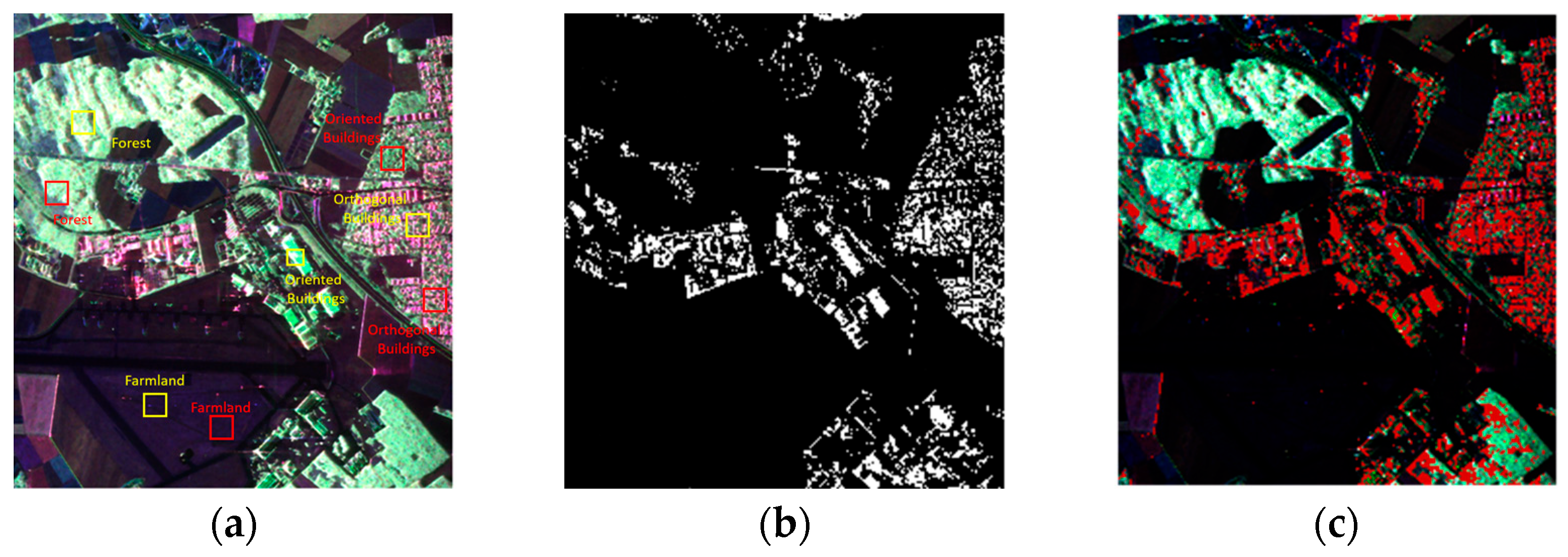
According to Section 2.5, the training sets and validation sets are selected as shown in Figure 5a, K = 9, and the extraction results for urban areas are shown in Figure 5b. In Figure 5, farmland, forests, orthogonal buildings, and oriented buildings are selected as typical features for extractor threshold selection, with the training sets marked by yellow rectangles and the validation sets marked by red rectangles. In order to analyze the validity of the building extraction results more intuitively, the building extraction results are superimposed onto the Pauli pseudo-color map, as shown in Figure 5c. It can be concluded that the building areas with various orientation angles, especially the building areas with large orientation angles, can be properly extracted. The extraction results can be used for subsequent decomposition processes.

Figure 5. (a) Training sets and validation sets selection of E-SAR data. (b) Build-up area extraction results. (c) Superimpose the extraction results on the Pauli pseudo-color map.

3.2. Decomposition Results

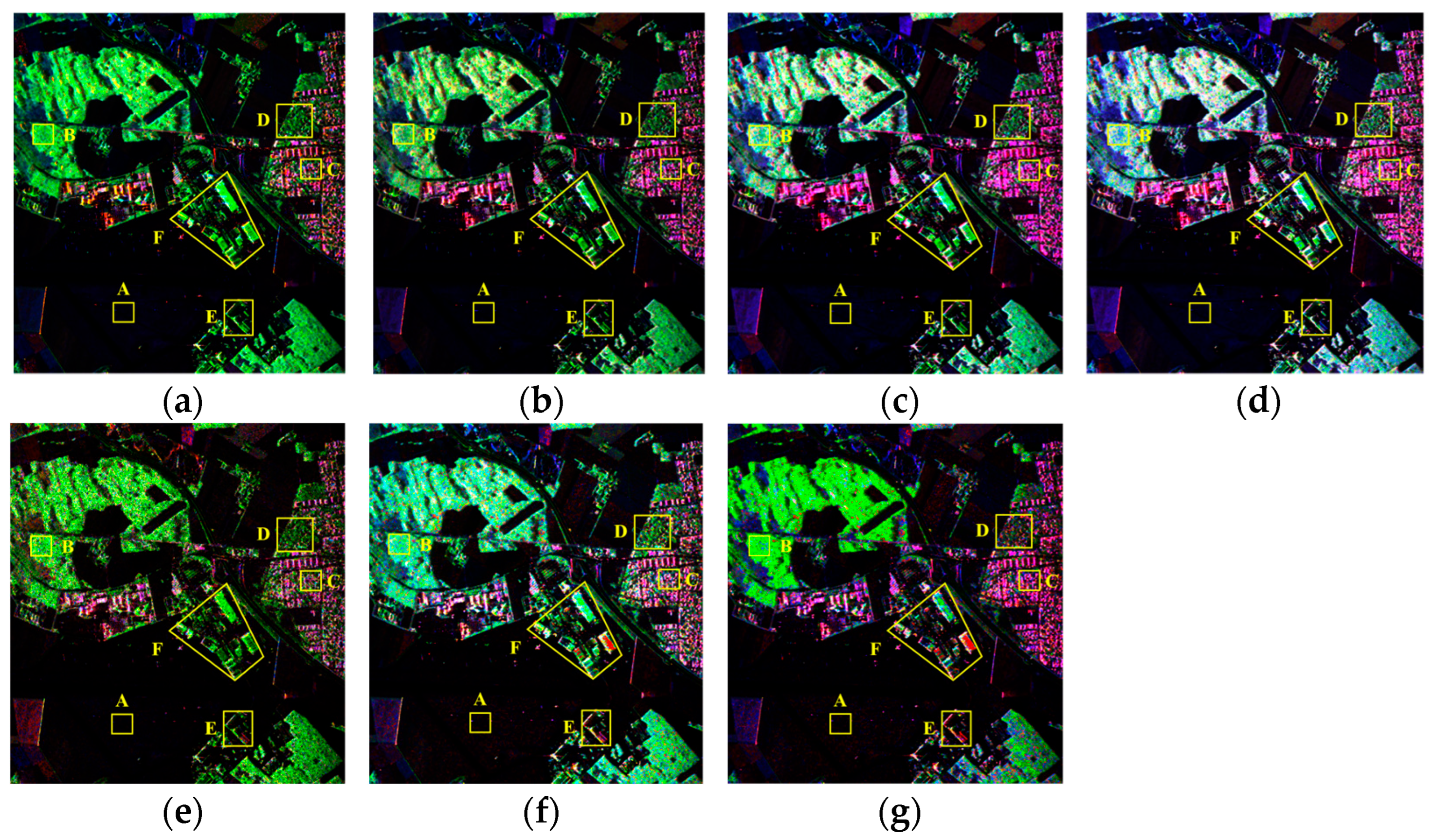
Figure 6g presents the comprehensive polarimetric decomposition map derived from MCSMRV. To assess the performance of the proposed method in oriented buildings, we compared the MCSMRV decomposition outcomes with those obtained through FDD, Y4R, G4U, ExG4URcc, MCSM, and MCSMs, as shown in Figure 6a–f. It is worth noting that the urban scattering ($P_u$, $P_u=P_d+P_c+P_w$ (where applicable components exist)), represented by the red color in the pseudo-color map, encompasses double-bounce scattering, helix scattering, and wire scattering components. In Figure 6, these seven methods accurately interpret the primary scattering mechanisms of airport runways, farmland, and vegetation areas. When compared to existing decomposition techniques, MCSMRV significantly diminishes the influence of volume scattering in building zones and the scattering mechanisms are logically interpreted.

Figure 6. The decomposition outcomes derived from various methodologies: (a) FDD, (b) Y4R, (c) G4U, (d) ExG4URcc, (e) MCSM, (f) MCSMs, and (g) MCSMRV (red: Urban scattering; green: Volume scattering; and blue: Surface scattering). A–F are the selected patches used to analyze the performance of the various decomposition methods in interpreting scattering mechanisms.

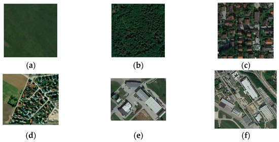
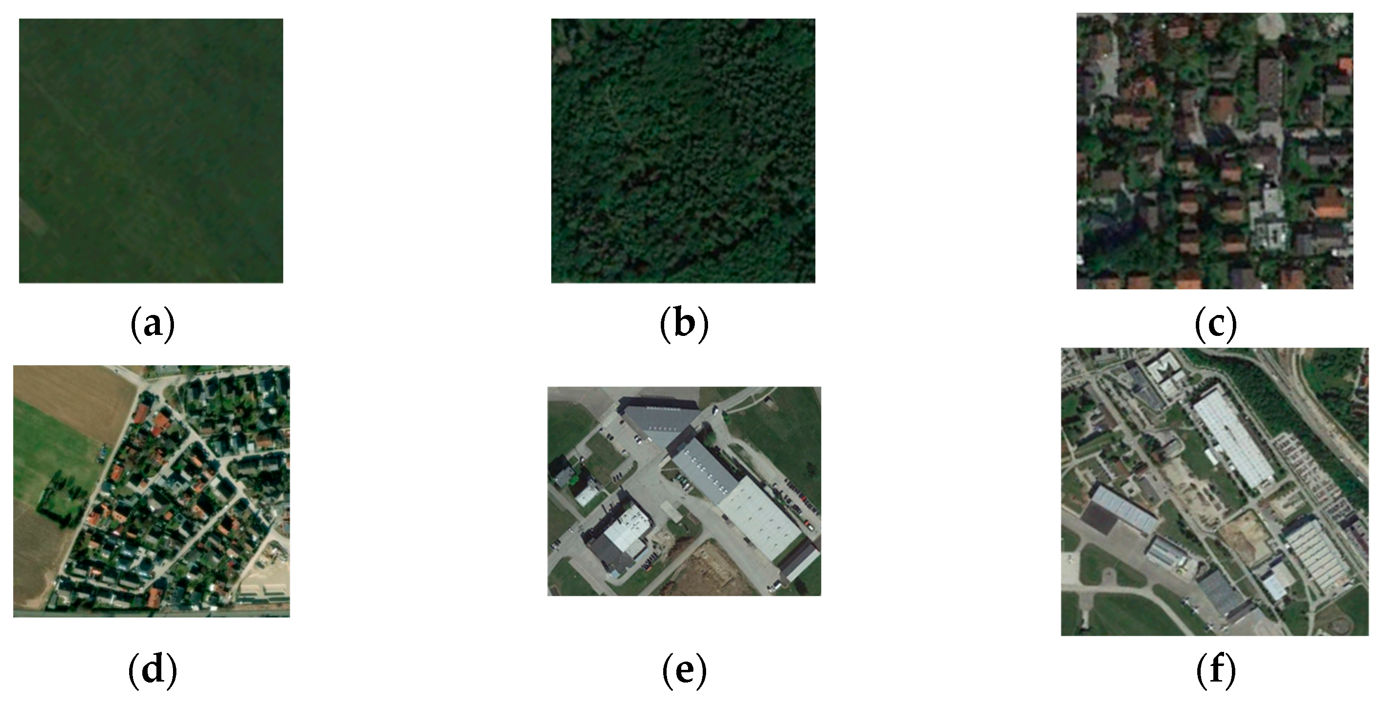
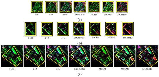
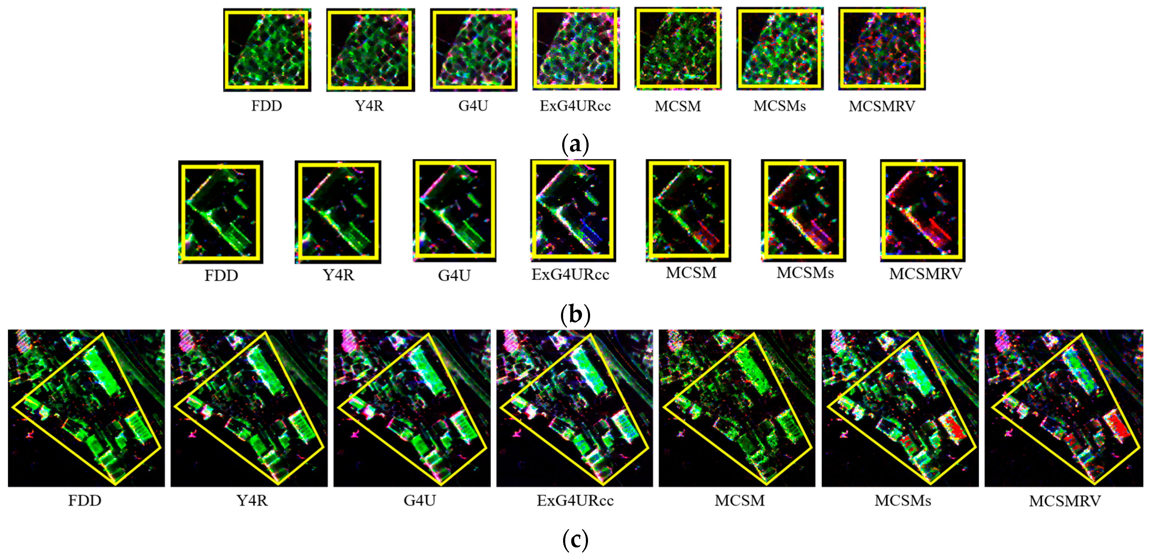
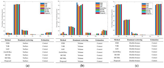
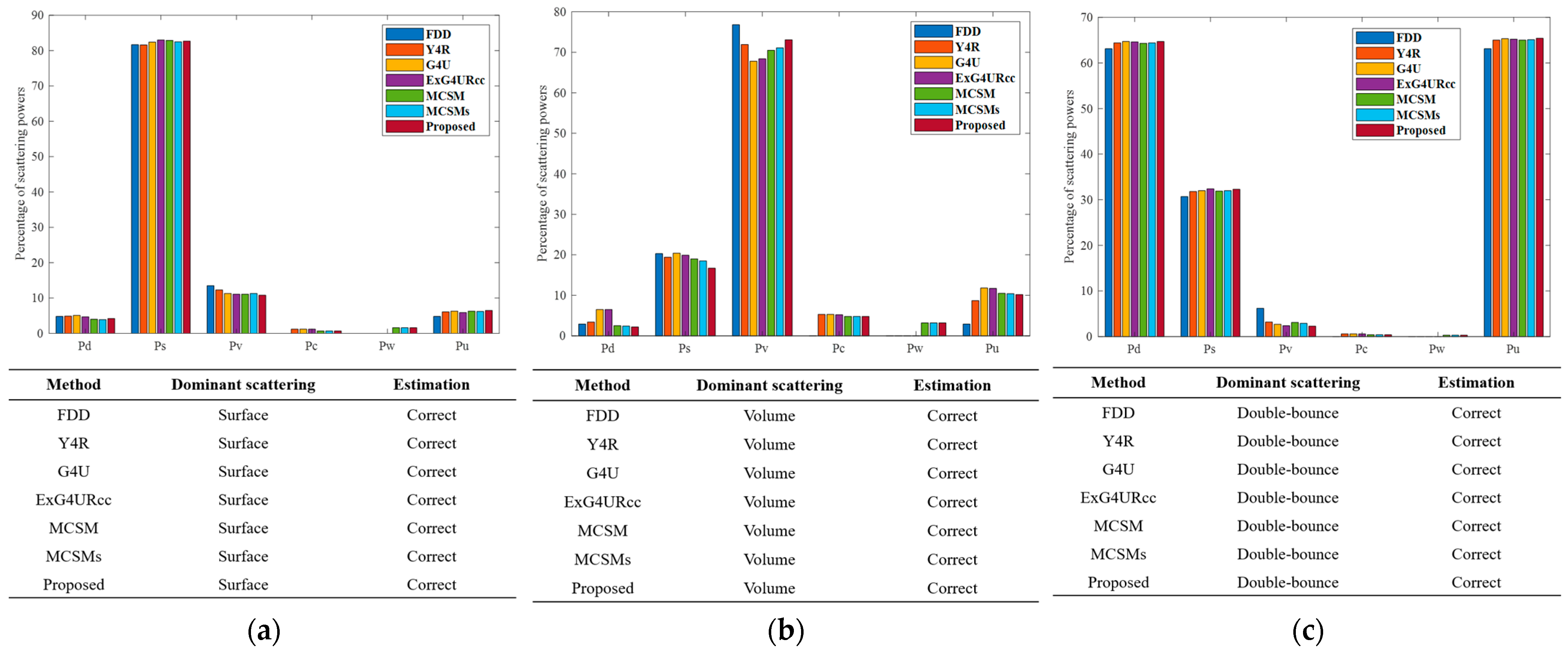
To assess the efficacy of MCSMRV quantitatively, six distinct regions, as depicted in Figure 6, were chosen for analysis. The corresponding optical images are presented in Figure 7, while enlarged decomposition images focusing on building zones with various orientations (patches D, E, and F) are shown in Figure 8. Specifically, patch A represents farmland, patch B represents forest, and patch C represents orthogonally oriented buildings. Figure 9 displays the decomposition maps for these patches, derived from aforementioned seven different methods. The results in Figure 9 indicate that all decomposition methods can effectively interpret the scattering mechanisms within patches A, B, and C. For instance, the primary scattering mechanism in vegetated areas is volume scattering; in farmland and runways, it is surface scattering; and in orthogonally oriented building areas, it is double-bounce scattering.

Figure 7. Optical images of patches (a) A, (b) B, (c) C, (d) D, (e) E, and (f) F.

Figure 8. Enlarged decomposition images of (a) patch D, (b) patch E, and (c) patch F.

Figure 9. Bar charts showing the percentage of each scattering component obtained via FDD, Y4R, G4U, ExG4URcc, MCSM, MCSMs, and MCSMRV. (a) Patch A, (b) Patch B, and (c) Patch C.

Regarding the farmland and runway, surface scattering plays a pivotal role, contributing 81.7%, 81.6%, 82.4%, 83.0%, 82.9%, 82.5%, and 82.7%, respectively, for FDD, Y4R, G4U, ExG4URcc, MCSM, MCSMs, and MCSMRV. In vegetated areas, volume scattering emerges as the primary mechanism, accounting for 76.8%, 71.9%, 67.8%, 68.4%, 70.5%, 71.1%, and 73.1%, respectively, for the aforementioned methods. In Patch C, where buildings are oriented orthogonally or nearly orthogonally to the LOS, double-bounce scattering is dominant, with percentages of 63.1%, 64.4%, 64.7%, 64.6%, 64.3%, 64.4%, and 64.7% for FDD, Y4R, G4U, ExG4URcc, MCSM, MCSMs, and MCSMRV, respectively. Moreover, urban scattering, encompassing double-bounce, helix, and wire scattering, can also be considered a primary mechanism in orthogonal building areas. The aforementioned decomposition techniques can all serve as tools for elucidating the dominant scattering mechanisms prevalent in vegetated regions, agricultural lands, and areas with perpendicular structures.

Patches D, E, and F represent building zones characterized by significant orientation angles. The rotation of these building zones results in an elevation of the cross-polarized component. When employing the MCSMRV method, these three regions exhibit a notably ‘redder’ appearance compared to images derived from existing decomposition techniques. The percentages of scattering power in these regions are detailed in Table 1, Table 2 and Table 3.

Table 1. Percentage of scattering power in patch D of Oberpfaffenhofen, Germany (%).

Methods	${\mathit{P}}_{\mathit{d}}$	${\mathit{P}}_{\mathit{s}}$	${\mathit{P}}_{\mathit{v}}$	${\mathit{P}}_{\mathit{c}}$	${\mathit{P}}_{\mathit{w}}$	Pu 1
FDD	12.9	50.7	36.6	-- 2	--	12.9
Y4R	13.0	50.8	30.2	6.0	--	19.0
G4U	13.4	51.7	28.9	6.0	--	19.4
ExG4URcc	13.5	57.4	23.1	6.0	--	19.5
MCSM	13.7	53.9	18.4	6.0	8.0	27.7
MCSMs	15.7	48.6	21.7	6.0	8.0	29.7
MCSMRV	19.4	54.3	12.3	6.0	8.0	33.4

¹ $P_u=P_d+P_c+P_w$ (where applicable components exist). ² “--” indicates that this decomposition technique does not include this scattering component.

Table 2. Percentage of scattering power in patch E of Oberpfaffenhofen, Germany (%).

Methods	${\mathit{P}}_{\mathit{d}}$	${\mathit{P}}_{\mathit{s}}$	${\mathit{P}}_{\mathit{v}}$	${\mathit{P}}_{\mathit{c}}$	${\mathit{P}}_{\mathit{w}}$	${\mathit{P}}_{\mathit{u}}$
FDD	11.5	27.6	60.9	--	--	11.5
Y4R	17.7	31.3	44.7	6.3	--	24.0
G4U	31.7	38.4	23.6	6.3	--	38.0
ExG4URcc	31.5	36.0	26.2	6.3	--	37.8
MCSM	26.2	32.9	30.8	4.4	5.7	36.3
MCSMs	26.9	33.2	29.8	4.4	5.7	37.0
MCSMRV	31.4	35.7	22.8	4.4	5.7	41.5

Table 3. Percentage of scattering power in patch F of Oberpfaffenhofen, Germany (%).

Methods	${\mathit{P}}_{\mathit{d}}$	${\mathit{P}}_{\mathit{s}}$	${\mathit{P}}_{\mathit{v}}$	${\mathit{P}}_{\mathit{c}}$	${\mathit{P}}_{\mathit{w}}$	${\mathit{P}}_{\mathit{u}}$
FDD	11.4	24.5	64.1	--	--	11.4
Y4R	12.0	39.3	42.2	6.5	--	18.5
G4U	14.8	42.1	36.6	6.5	--	21.3
ExG4URcc	15.9	42.5	35.1	6.5	--	22.4
MCSM	11.8	35.7	38.8	3.3	10.4	25.5
MCSMs	13.2	36.4	36.7	3.3	10.4	26.9
MCSMRV	17.2	41.3	27.8	3.3	10.4	30.9

Regarding area D, the $P_u$ component, which encompasses double-bounce, wire, and helix scattering, accounts for varying percentages: 12.9% for FDD, 19.0% for Y4R, 19.4% for G4U, 19.5% for ExG4URcc, 27.7% for MCSM, 29.7% for MCSMs, and 33.4% for MCSMRV. The primary scattering mechanisms in this area are surface and urban scattering. Consequently, MCSMRV offers an advantage over existing decomposition methods in interpreting the scattering characteristics of building zones with substantial orientation angles.

In the case of patch E, the angle of orientation surpasses that of patch D. The results of the analysis indicate that urban scattering comprises 11.5% in FDD, 24.0% in Y4R, 38.0% in G4U, 37.8% in ExG4URcc, 36.3% in MCSM, 37.0% in MCSMs, and 41.5% in MCSMRV. As per Table 2, there is a shift from reduced volume scattering to surface and double-bounce scattering, accurately depicting the scattering mechanism in building zones. Figure 8b illustrates that MCSMRV decomposition results in patch E accurately reflect the presence of buildings, depicted in red, aligning with ground truth.

In patch F, where buildings have an orientation angle of approximately 45°, traditional volume scattering models and the OAC operation are ineffective. The percentages of urban scattering are 11.4% for FDD, 18.5% for Y4R, 21.3% for G4U, 22.4% for ExG4URcc, 25.5% for MCSM, 26.9% for MCSMs, and 30.9% for MCSMRV. When compared to existing polarimetric decomposition methods, MCSMRV reduces the volume scattering component by 36.3%, 14.4%, 8.8%, 7.3%, 11.0%, and 8.9%. This reduction in volume scattering power shifts towards surface and urban scattering, providing a more accurate depiction of the scattering mechanisms in this oriented building area. Consequently, MCSMRV is well-suited for describing the scattering properties of urban areas featuring substantial orientation angles. The findings depicted in Figure 8c further validate that MCSMRV can accurately represent the primary scattering mechanism within this region.

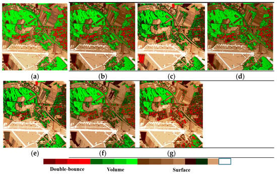
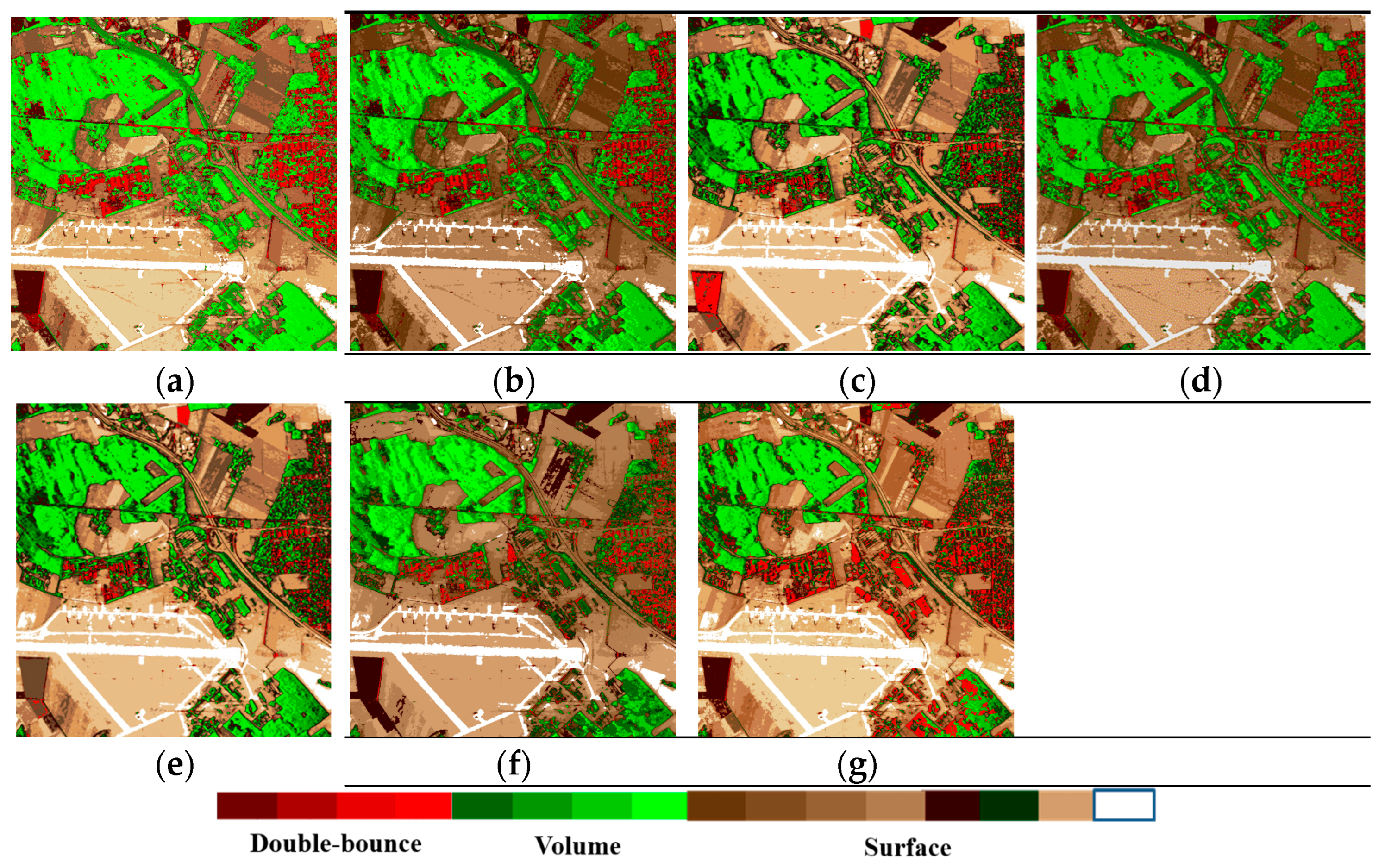
To quantitatively describe the accuracy of the decomposition results, we utilized the percentage of each scattering component, using the dominance of the dominant scattering mechanism as the main criterion, to obtain the image classification results, as shown in Figure 10. As can be seen from the classification results shown in Figure 10, the classification results obtained by the proposed method are more consistent with the actual land cover types: for areas such as bare soil, farmland, vegetation, runways and orthogonal buildings, all methods are able to classify them correctly; however, the proposed method is better at preserving contour and boundary information for different land cover types; For areas containing oblique buildings, particularly those with steep angles of inclination, the proposed method achieves superior classification results. Oriented buildings are correctly classified, and the issue of confusion between building and vegetation areas is effectively mitigated. By comparing these results with the ground truth, we can quantitatively assess the accuracy of the decomposition results. As shown in Table 4, compared with existing decomposition methods, the proposed method achieves higher overall accuracy and Kappa coefficients, provides a better explanation of the scattering mechanisms of surface features, and is more effective at distinguishing between different types of surface features.

Figure 10. Classification results derived from the dominant scattering mechanism of each pixel using different methodologies: (a) FDD, (b) Y4R, (c) G4U, (d) ExG4URcc, (e) MCSM, (f) MCSMs, and (g) MCSMRV.

Table 4. Quantitative statistical analysis of the accuracy of scattering mechanism interpretation results.

Methods	FDD	Y4R	G4U	ExG4URcc	MCSM	MCSMs	MCSMRV
Overall accuracy (%)	67.08	74.55	77.49	80.22	76.33	81.07	90.52
Kappa coefficient	0.5086	0.5941	0.6337	0.7259	0.6842	0.7501	0.8102

When compared to three-component, four-component, and multiple-component decomposition methods, MCSMRV yields superior results across various terrain types, particularly in building areas. This can be attributed to the following reasons: (1) Unlike traditional and enhanced three-component and four-component decomposition methods, MCSMRV divides the coherency matrix into five components, effectively demonstrating the significance of wire scattering in building areas. Furthermore, MCSMRV incorporates a novel deorientation technique, which compensates for the rotation angle of buildings in the image, thereby enhancing the understanding of scattering processes across diverse land cover types. Compared with the FDD method, MCSMRV achieved a 38.1% reduction in Patch E (Table 2) and a 36.3% reduction in Patch F (Table 3). (2) Unlike current multi-component decomposition techniques, MCSMRV employs sophisticated volume scattering models and interferometric data to provide a more nuanced understanding of volume scattering across various land cover types. Consequently, the volume scattering power in building areas is reasonably reduced. Compared with the MCSM method, MCSMRV achieved an 8% reduction in Patch E (Table 2) and an 11% reduction in Patch F (Table 3). Additionally, MCSMRV uses a branch condition to distinguish between building and vegetation areas, resulting in more accurate initial divisions and improved decomposition outcomes. Therefore, MCSMRV stands out in addressing the challenge of orientation variability and precisely delineating the scattering properties of diverse terrain types.

Drawing from Table 1, Table 2 and Table 3, it is evident that MCSMRV outperforms existing decomposition methods by enhancing urban scattering while significantly diminishing volume scattering. Specifically, the urban term $P_u$ plays a pivotal role in building areas, particularly those with substantial orientation angles, serving as a crucial indicator of the scattering mechanism. Furthermore, MCSMRV leverages interferometric information to mitigate the influence of volume scattering. For oriented urban areas, particularly those with significant orientation angles, MCSMRV provides a more precise depiction of the scattering processes across various land covers by utilizing interferometric data and enhanced volume scattering models. This, in turn, helps to overcome the issue of orientation variability.

Moreover, the proportion of pixels exhibiting negative scattering powers serves as another vital metric to assess the effectiveness of the method. Prior computation of the volume scattering component can lead to negative values for some double-bounce and surface scattering terms. Table 5 presents the percentages of negative scattering powers obtained through FDD, Y4R, G4U, ExG4URcc, MCSM, MCSMs, and MCSMRV. Upon comparing MCSMRV with the six existing decomposition methods in Table 5, it is evident that MCSMRV significantly reduces the number of pixels with negative scattering powers. Therefore, MCSMRV can effectively decrease the occurrence of negative power pixels.

Table 5. Proportion of pixels with negative scattering values in the Oberpfaffenhofen, Germany.

Methods	FDD	Y4R	G4U	ExG4URcc	MCSM	MCSMs	MCSMRV
Percentage of negative scattering powers (%)	27.4	26.1	21.5	19.4	22.7	20.0	19.1

3.3. PolInSAR Data Obtained by AIR

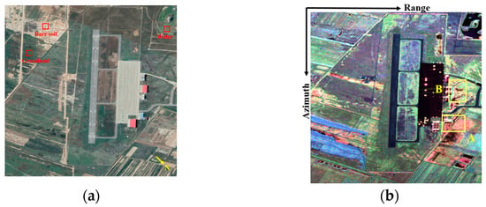
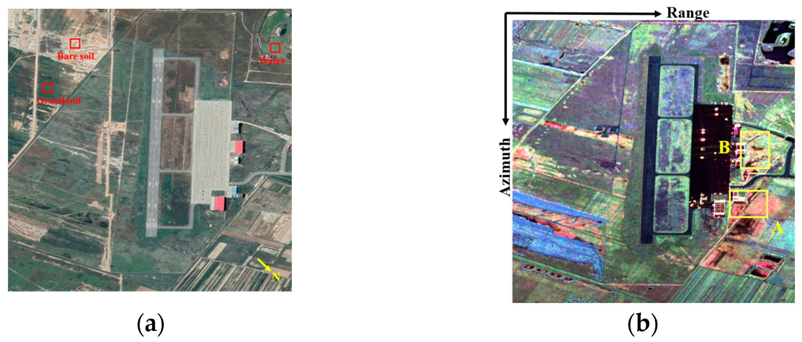
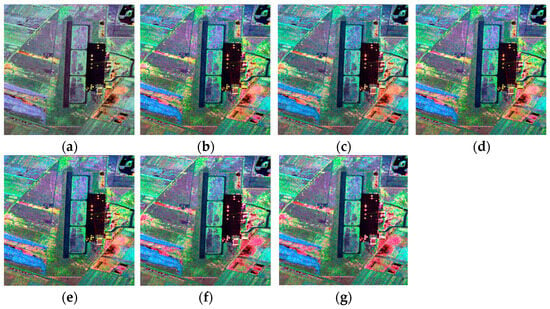
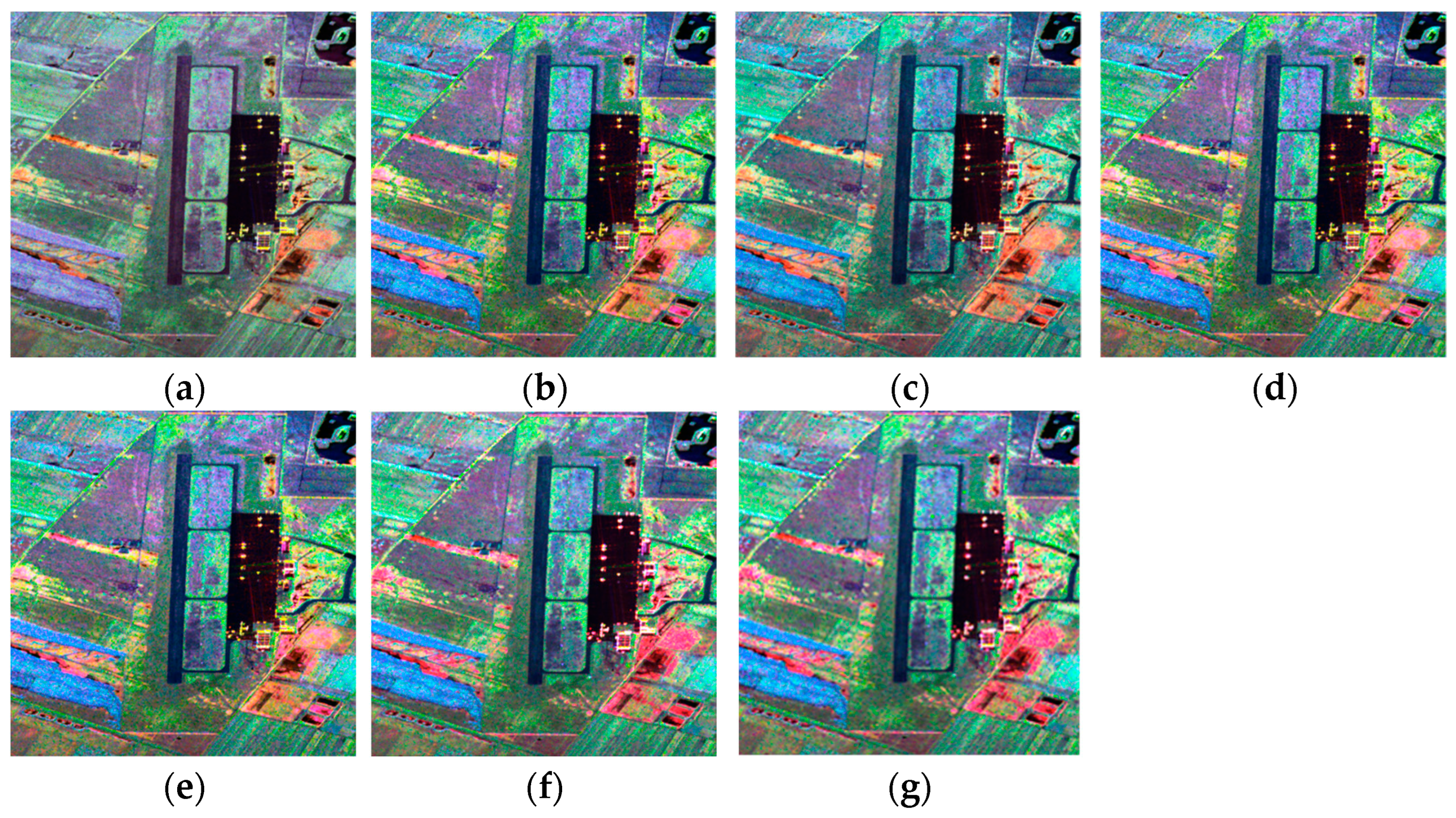
To underscore the reliability of MCSMRV, we conducted experiments using airborne C-band PolInSAR data acquired by the AIR over Xi’an, China. This dataset comprises an image of 2479 × 2473 pixels, with simultaneous collection of master and slave data. The image has an incidence angle of approximately 40° and a spatial resolution of 2.43 m × 2.08 m. The wavelength is appropriate 6 cm. Figure 11 displays the optical image alongside its corresponding color-coded Pauli image. There are few terrain types in the image and K = 6. The decomposition results obtained via aforementioned seven methods are shown in Figure 12.

Figure 11. Airborne C-band SAR images over Xi’an, China. (a) An optical image sourced from Google Earth. (b) The color-coded Pauli decomposition results (red: $T_{22}$ term; green: $T_{33}$ term; and blue: $T_{11}$ term). A and B are the selected patches used to analyze the performance of the various decomposition methods in interpreting scattering mechanisms.

Figure 12. The outcomes derived from (a) FDD, (b) Y4R, (c) G4U, (d) ExG4URcc, (e) MCSM, (f) MCSMs, and (g) MCSMRV (red: Urban scattering; green: Volume scattering; and blue: Surface scattering).

To demonstrate that the improvements achieved by the proposed method are consistent across different land cover types or datasets, we first selected water, grassland, and bare soil areas to verify the algorithm’s robustness, as shown in Figure 11a. As can be seen from Figure 12, the dominant scattering mechanisms identified in the decomposition results for these three areas are consistent across different methods; the image interpretation and pseudo-color results are similar, and all algorithms yield satisfactory interpretation results in these areas.

For quantitative evaluation, two specific areas marked as patches A and B in Figure 11b were selected. The scattering power contributions for these ROIs, derived from the decomposition process, are outlined in Table 6 and Table 7. In the study locations, the variety of land covers is limited, and the building zones are aligned or nearly aligned with the LOS. Areas with significant orientation angles exhibit OVS, resulting in a higher proportion of volume scattering power. Utilizing conventional decomposition techniques in these regions presents challenges. However, Table 6 and Table 7 indicate that, when MCSMRV is applied, the volume scattering power in the ROIs is notably reduced, while the urban and surface scattering components increase correspondingly. The decomposition outcomes achieved with MCSMRV effectively mitigate the impact of OVS. This suggests that interferometric information and refined volume scattering models are crucial for understanding the scattering behavior of building zones, particularly those with large angles.

Table 6. Percentage of scattering power in patch A of Xi’an, China (%).

Methods	${\mathit{P}}_{\mathit{d}}$	${\mathit{P}}_{\mathit{s}}$	${\mathit{P}}_{\mathit{v}}$	${\mathit{P}}_{\mathit{c}}$	${\mathit{P}}_{\mathit{w}}$	${\mathit{P}}_{\mathit{u}}$
FDD	40.2	28.9	30.9	--	--	40.2
Y4R	41.4	29.7	26.4	2.5	--	43.9
G4U	42.1	31.1	24.3	2.5	--	44.6
ExG4URcc	42.2	32.2	23.1	2.5	--	44.7
MCSM	41.7	30.2	24.3	1.1	2.7	45.5
MCSMs	41.9	30.3	24.0	1.1	2.7	45.7
MCSMRV	43.6	31.5	21.1	1.1	2.7	47.4

Table 7. Percentage of scattering power in patch B of Xi’an, China (%).

Methods	${\mathit{P}}_{\mathit{d}}$	${\mathit{P}}_{\mathit{s}}$	${\mathit{P}}_{\mathit{v}}$	${\mathit{P}}_{\mathit{c}}$	${\mathit{P}}_{\mathit{w}}$	${\mathit{P}}_{\mathit{u}}$
FDD	11.7	30.9	57.4	--	--	11.7
Y4R	12.5	31.2	53.1	3.2	--	15.7
G4U	13.9	31.5	51.4	3.2	--	17.1
ExG4URcc	14.0	33.5	49.3	3.2	--	17.2
MCSM	12.9	30.7	51.8	1.4	3.2	17.5
MCSMs	13.2	30.3	51.9	1.4	3.2	17.8
MCSMRV	16.3	32.1	47.0	1.4	3.2	20.9

Similarly, the effectiveness of this method was assessed by calculating the proportion of pixels contributing to the negative scattered power. Table 8 presents the percentages of negative scattering powers obtained through FDD, Y4R, G4U, ExG4URcc, MCSM, MCSMs, and MCSMRV. Upon comparing MCSMRV with the six existing decomposition methods in Table 8, we can draw the same conclusion as from the ESAR data: MCSMRV is effective in reducing the frequency of negative power pixels.

Table 8. Proportion of pixels with negative scattering values in Xi’an, China.

Methods	FDD	Y4R	G4U	ExG4URcc	MCSM	MCSMs	MCSMRV
Percentage of negative scattering powers (%)	15.74	13.62	13.49	12.17	14.02	12.40	11.49

4. Conclusions

In this research paper, we introduce a model-driven technique for decomposing multiple components in PolInSAR data, leveraging enhanced volume scattering models to elucidate the scattering mechanisms of diverse land cover types. Our proposed method, referred to as MCSMRV, incorporates an innovative deorientation approach to account for rotational angles. This technique can adjust both the angle formed between a building and the SAR azimuth direction, as well as the angle between the building and the SAR LOS. To further refine our volume scattering models, we utilized a similarity parameter known as PISP. Additionally, we propose the RWMM as a criterion for selecting the most suitable volume scattering model adaptively. Two datasets collected in different bands were utilized to validate the effectiveness of MCSMRV. The experimental findings confirm that the decomposition results obtained through MCSMRV offer profound understanding into the scattering mechanisms of diverse land covers and address the limitations of OVS. Specifically, for urban areas, especially large oriented buildings, the volume scattering power is significantly minimized. Consequently, buildings with distinct orientations can be clearly distinguished from vegetation. In summary, MCSMRV represents a potent decomposition method for analyzing PolInSAR data.

Building upon the methodology proposed in this paper, subsequent research will proceed in two distinct phases: firstly, expanding the number of scattering mechanisms employed in the decomposition process to maximize the utilization of comprehensive coherency matrix information, the number of decomposition components can be expanded to nine, thereby better corresponding to the nine elements of the coherency matrix; secondly, further extending the volume scattering models to more accurately characterize the volume scattering power of diverse terrain features. In addition, once spaceborne PolInSAR data are publicly accessible, further validation of MCSMRV on large-area imagery will be conducted to confirm its robustness.

References

- Sharma, J.J.; Hajnsek, I.; Papathanassiou, K.P.; Moreira, A. Polarimetric Decomposition over Glacier Ice Using Long-Wavelength Airborne PolSAR. IEEE Trans. Geosci. Remote Sens. 2011, 49, 519–535. [Google Scholar] [CrossRef] [Scilit]
- Zhang, X.; Dierking, W.; Zhang, J.; Meng, J. A Polarimetric Decomposition Method for Ice in the BoHai Sea Using C-Band PolSAR Data. IEEE J. Sel. Top. Appl. Earth Obs. Remote Sens. 2015, 8, 47–66. [Google Scholar] [CrossRef] [Scilit]
- Hajnsek, I.; Jagdhuber, T.; Schon, H.; Papathanassiou, K.P. Potential of Estimating Soil Moisture Under Vegetation Cover by Means of PolSAR. IEEE Trans. Geosci. Remote Sens. 2009, 47, 442–454. [Google Scholar] [CrossRef] [Scilit]
- Jagdhuber, T.; Hajnsek, I.; Papathanassiou, K.P. An Iterative Generalized Hybrid Decomposition for Soil Moisture Retrieval Under Vegetation Cover Using fully Polarimetric SAR. IEEE J. Sel. Top. Appl. Earth Obs. Remote Sens. 2015, 8, 3911–3922. [Google Scholar] [CrossRef] [Scilit]
- Martino, G.D.; Iodice, A.; Natale, A.; Riccio, D. Polarimetric Two-Scale Two-Component Model for the Retrieval of Soil Moisture Under Moderate Vegetation via L-Band SAR Data. IEEE Trans. Geosci. Remote Sens. 2016, 54, 2470–2491. [Google Scholar] [CrossRef] [Scilit]
- Wang, H.; Magagi, R.; Goïta, K.; Jagdhuber, T. Refining a Polarimetric Decomposition of Multi-Angular UAVSAR Time Series for Soil Moisture Retrieval over Low and High Vegetated Agricultural Fields. IEEE J. Sel. Top. Appl. Earth Obs. Remote Sens. 2019, 12, 1431–1450. [Google Scholar] [CrossRef] [Scilit]
- Chen, S.W.; Sato, M. Tsunami Damage Investigation of Built-Up Areas Using Multitemporal Spaceborne Full Polarimetric SAR Images. IEEE Trans. Geosci. Remote Sens. 2013, 51, 1985–1997. [Google Scholar] [CrossRef] [Scilit]
- Ji, Y.; Sumantyo, J.T.S.; Chua, M.Y.; Waqar, M.M. Earthquake/Tsunami Damage Level Mapping of Urban Areas Using Full Polarimetric SAR Data. IEEE J. Sel. Top. Appl. Earth Obs. Remote Sens. 2018, 11, 2296–2309. [Google Scholar] [CrossRef] [Scilit]
- Rajat; Avtar, R. Development of Four Component Scattering Power Decomposition Technique for Dual Polarization SAR Data. J. Indian Soc. Remote Sens. 2024, 52, 2611–2623. [Google Scholar] [CrossRef] [Scilit]
- Cloude, S.R.; Pottier, E. An Entropy Based Classification Scheme for Land Applications of Polarimetric SAR. IEEE Trans. Geosci. Remote Sens. 1997, 35, 68–78. [Google Scholar] [CrossRef] [Scilit]
- Touzi, R. Target Scattering Decomposition in Terms of Roll-Invariant Target Parameters. IEEE Trans. Geosci. Remote Sens. 2007, 45, 73–84. [Google Scholar]
- Freeman, A.; Durden, S.L. A Three-Component Scattering Model for Polarimetric SAR Data. IEEE Trans. Geosci. Remote Sens. 1998, 36, 963–973. [Google Scholar] [CrossRef] [Scilit]
- Yamaguchi, Y.; Moriyama, T.; Ishido, M.; Yamada, H. Four-Component Scattering Model for Polarimetric SAR Image Decomposition. IEEE Trans. Geosci. Remote Sens. 2005, 43, 1699–1706. [Google Scholar] [CrossRef] [Scilit]
- Zhang, L.; Zou, B.; Zhang, Y. Multiple-Component Scattering Model for Polarimetric SAR Image Decomposition. IEEE Geosci. Remote Sens. Lett. 2008, 5, 603–607. [Google Scholar] [CrossRef] [Scilit]
- Sato, A.; Yamaguchi, Y.; Singh, G.; Park, S.E. Four-Component Scattering Power Decomposition with Extended Volume Scattering Model. IEEE Geosci. Remote Sens. Lett. 2012, 9, 166–170. [Google Scholar] [CrossRef] [Scilit]
- Singh, G.; Yamaguchi, Y.; Park, S.E. General Four-Component Scattering Power Decomposition with Unitary Transformation of Coherency Matrix. IEEE Trans. Geosci. Remote Sens. 2013, 51, 3014–3022. [Google Scholar]
- Singh, G.; Yamaguchi, Y. Model-Based Six-Component Scattering Matrix Power Decomposition. IEEE Trans. Geosci. Remote Sens. 2018, 56, 5687–5704. [Google Scholar] [CrossRef] [Scilit]
- Singh, G.; Malik, R.; Mohanty, S.; Rathore, V.S.; Yamada, K.; Umemura, M.; Yamaguchi, Y. Seven-Component Scattering Power Decomposition of PolSAR Coherency Matrix. IEEE Trans. Geosci. Remote Sens. 2019, 57, 8371–8382. [Google Scholar] [CrossRef] [Scilit]
- Dey, S.; Bhattacharya, A.; Frery, A.C.; López-Martínez, C.; Rao, Y.S. A Model-Free Four Component Scattering Power Decomposition for Polarimetric SAR Data. IEEE J. Sel. Top. Appl. Earth Obs. Remote Sens. 2021, 14, 3887–3902. [Google Scholar] [CrossRef] [Scilit]
- Yamaguchi, Y.; Sato, A.; Boerner, W.M.; Sato, R.; Yamada, H. Four-Component Scattering Power Decomposition with Rotation of Coherency Matrix. IEEE Trans. Geosci. Remote Sens. 2011, 49, 2251–2258. [Google Scholar]
- Xiang, D.; Wang, W.; Tang, T.; Su, Y. Multiple-Component Polarimetric Decomposition with New Volume Scattering Models for PolSAR Urban Areas. IET Radar Sonar Navig. 2017, 11, 410–419. [Google Scholar] [CrossRef] [Scilit]
- Quan, S.; Xiang, D.; Xiong, B.; Hu, C.; Kuang, G. A Hierarchical Extension of General Four-Component Scattering Power Decomposition. Remote Sens. 2017, 9, 856. [Google Scholar] [CrossRef] [Scilit]
- Xiang, D.; Ban, Y.; Su, Y. Model-Based Decomposition with Cross Scattering for Polarimetric SAR Urban Areas. IEEE Geosci. Remote Sens. Lett. 2015, 12, 2496–2500. [Google Scholar] [CrossRef] [Scilit]
- Dey, S.; Bhattacharya, A.; Ratha, D.; Mandal, D.; Frery, A.C. Target Characterization and Scattering Power Decomposition for Full and Compact Polarimetric SAR Data. IEEE Trans. Geosci. Remote Sens. 2021, 59, 3981–3998. [Google Scholar] [CrossRef] [Scilit]
- Chen, S.W.; Ohki, M.; Shimada, M.; Sato, M. Deorientation Effect Investigation for Model-Based Decomposition over Oriented Built-Up Areas. IEEE Geosci. Remote Sens. Lett. 2013, 10, 273–277. [Google Scholar] [CrossRef] [Scilit]
- Sun, X.; Song, H.; Wang, R.; Li, N. High-Resolution Polarimetric SAR Image Decomposition of Urban Areas Based on a POA Correction Method. Remote Sens. Lett. 2018, 9, 363–372. [Google Scholar] [CrossRef] [Scilit]
- Deng, L.; Yan, Y.N. Improving the Yamaguchi4 Decomposition Method Using Selective Polarization Orientation Compensation. Can. J. Remote Sens. 2016, 42, 125–135. [Google Scholar] [CrossRef] [Scilit]
- Lee, J.S.; Schuler, D.L.; Ainsworth, T.L. Polarimetric SAR Data Compensation for Terrain Azimuth Slope Variation. IEEE Trans. Geosci. Remote Sens. 2000, 38, 2153–2163. [Google Scholar]
- Li, H.; Chen, J.; Li, Q.; Wu, G.; Chen, J. Mitigation of Reflection Symmetry Assumption and Negative Power Problems for the Model-Based Decomposition. IEEE Trans. Geosci. Remote Sens. 2016, 54, 7261–7271. [Google Scholar] [CrossRef] [Scilit]
- Lee, J.S.; Ainsworth, T.L.; Wang, Y. Polarization Orientation Angle and Polarimetric SAR Scattering Characteristics of Steep Terrain. IEEE Trans. Geosci. Remote Sens. 2018, 56, 7272–7281. [Google Scholar] [CrossRef] [Scilit]
- Li, H.; Li, Q.; Wu, G.; Chen, J.; Liang, S. The Impacts of Building Orientation on Polarimetric Orientation Angle Estimation and Model-Based Decomposition for Multilook Polarimetric SAR Data in Urban Areas. IEEE Trans. Geosci. Remote Sens. 2016, 54, 5520–5532. [Google Scholar] [CrossRef]
- Wang, Y.; Yu, W.; Hou, W. Five-Component Decomposition Methods of Polarimetric SAR and Polarimetric SAR Interferometry Using Coupling Scattering Mechanisms. IEEE J. Sel. Top. Appl. Earth Obs. Remote Sens. 2021, 14, 6662–6676. [Google Scholar] [CrossRef] [Scilit]
- Li, P.; Liu, X.; Zhang, H.; Liu, D.; Wang, R. A Novel Technique for Inversion of Rotation Angles in Built-Up Areas. IEEE Geosci. Remote Sens. Lett. 2022, 19, 1–5. [Google Scholar] [CrossRef] [Scilit]
- Malik, R.; Singh, G.; Dikshit, O.; Yamaguchi, Y. Model-Based Nine-Component Scattering Matrix Power Decomposition. IEEE Geosci. Remote Sens. Lett. 2024, 21, 1–5. [Google Scholar] [CrossRef] [Scilit]
- Bhattacharya, A.; Singh, G.; Manickam, S.; Yamaguchi, Y. An Adaptive General Four-Component Scattering Power Decomposition with Unitary Transformation of Coherency Matrix (AG4U). IEEE Geosci. Remote Sens. Lett. 2015, 12, 2110–2114. [Google Scholar] [CrossRef] [Scilit]
- Xiang, D.; Tang, T.; Ban, Y.; Su, Y.; Kuang, G. Unsupervised Polarimetric SAR Urban Area Classification Based on Model-Based Decomposition with cross scattering. ISPRS J. Photogramm. Remote Sens. 2016, 116, 86–100. [Google Scholar] [CrossRef] [Scilit]
- Cloude, S.R.; Papathanassiou, K.P. Polarimetric SAR Interferometry. IEEE Trans. Geosci. Remote Sens. 1998, 36, 1551–1565. [Google Scholar] [CrossRef] [Scilit]
- Chen, S.W.; Wang, X.S.; Li, Y.Z.; Sato, M. Adaptive Model-Based Polarimetric Decomposition Using PolInSAR Coherence. IEEE Trans. Geosci. Remote Sens. 2014, 52, 1705–1718. [Google Scholar] [CrossRef] [Scilit]
- Wang, Y.; Yu, W.; Liu, X.; Wang, C. A Hierarchical Extended Multiple-Component Scattering Decomposition of Polarimetric SAR Interferometry. IEEE Geosci. Remote Sens. Lett. 2020, 17, 1193–1197. [Google Scholar] [CrossRef] [Scilit]
- Kumar, A.; Giusti, E.; Mancuso, F.; Ghio, S.; Lupidi, A.; Martorella, M. Three-Dimensional Polarimetric INISAR Imaging of Non-Cooperative Targets. IEEE Trans. Comput. Imaging 2023, 9, 210–223. [Google Scholar] [CrossRef] [Scilit]
- Zhuang, D.; Zhang, L.; Zou, B. Iterative PolInSAR Target Decomposition for Scattering Characterization and Building Detection. IEEE J. Sel. Top. Appl. Earth Obs. Remote Sens. 2025, 18, 9211–9229. [Google Scholar] [CrossRef] [Scilit]
- Ohki, M.; Abe, T.; Tadono, T.; Shimada, M. Landslide Detection in Mountainous Forest Areas Using Polarimetry and Interferometric Coherence. Earth Planets Space 2020, 72, 67. [Google Scholar] [CrossRef] [Scilit]
- Wang, Y.; Yu, W.; Wang, C.; Liu, X. A Modified Four-Component Decomposition Method with Refined Volume Scattering Models. IEEE J. Sel. Top. Appl. Earth Obs. Remote Sens. 2020, 13, 1946–1958. [Google Scholar] [CrossRef] [Scilit]
- Yang, J.; Peng, Y.N.; Lin, S.M. Similarity Between Two Scattering Matrices. Electron. Lett. 2001, 37, 193–194. [Google Scholar] [CrossRef] [Scilit]
- Ohki, M.; Shimada, M. Large-Area Land Use and Land Cover Classification with Quad, Compact, and Dual Polarization SAR Data by PALSAR-2. IEEE Trans. Geosci. Remote Sens. 2018, 56, 5550–5557. [Google Scholar] [CrossRef] [Scilit]
Disclaimer/Publisher’s Note: The statements, opinions and data contained in all publications are solely those of the individual author(s) and contributor(s) and not of MDPI and/or the editor(s). MDPI and/or the editor(s) disclaim responsibility for any injury to people or property resulting from any ideas, methods, instructions or products referred to in the content. |
© 2026 by the authors. Licensee MDPI, Basel, Switzerland. This article is an open access article distributed under the terms and conditions of the Creative Commons Attribution (CC BY) license.