


Highlights
What are the main findings?
- Hydrological loading dominates seasonal GNSS vertical displacements across Southwest China, with pronounced spatial heterogeneity driven by topography and hydro-climatic gradients.
- EOF analysis reveals a dipole pattern linked to the moisture-blocking effect of the Hengduan Mountains, while the eastern Sichuan Basin shows anomalous atmospheric dominance.
- Three distinct crustal response regimes are identified: rapid elastic deformation on the Tibetan Plateau, intermediate delays in Yunnan, and strong hysteresis in the Sichuan Basin due to groundwater diffusion and poroelastic effects.
What are the implications of the main findings?
- Local hydrogeological dynamics, such as karst in Yunnan and poroelastic processes in Sichuan, critically modulate GNSS vertical deformation beyond simple elastic loading models.
- These findings provide new insights for improving environmental loading corrections and GNSS data processing in complex mountainous regions with heterogeneous hydrogeology.
Abstract
Environmental loading is a major driver of nonlinear GNSS vertical displacements, yet its spatiotemporal heterogeneity remains insufficiently understood in regions with complex topography. In this study, we investigate the environmental loading effects on GNSS vertical motions across Southwest China using observations from a network of 66 stations. Singular Spectrum Analysis (SSA) and Empirical Orthogonal Function (EOF) analysis were applied to extract annual signals, while component-wise RMS reduction quantified hydrological and atmospheric loading contributions. Spatial statistical analysis, cross-wavelet transform, and k-means clustering examined correlation patterns and phase hysteresis between GNSS observations and modeled loads. Results show that hydrological loading dominates seasonal vertical oscillations, but crustal responses exhibit pronounced spatial heterogeneity controlled by regional topography and hydro-climatic gradients. EOF analysis reveals a dipole pattern induced by the Hengduan Mountains’moisture-blocking effect. Atmospheric loading anomalously dominates the eastern Sichuan Basin, whereas Yunnan displays strong amplitudes with high heterogeneity due to karst hydrogeology. Phase analysis identifies three distinct regimes: a rapid elastic response on the Tibetan Plateau, (with the lag of ~20 ± 5 days, correlation coefficient R ≈ 0.65), intermediate delays in Yunnan (~60 ± 5 days, R ≈ 0.58), and pronounced hysteresis in the Sichuan Basin (~105 ± 5 days, R ≈ 0.38) linked to slow groundwater diffusion and poroelastic processes. These findings highlight the critical role of local hydrogeological dynamics in modulating GNSS vertical deformation and provide new insights for improving environmental loading corrections in complex mountainous regions.
1. Introduction
Global Navigation Satellite System (GNSS) coordinate time series are fundamental for monitoring crustal deformation, tectonic plate motion, and regional geodynamics [1]. However, these time series invariably contain nonlinear variations, particularly significant seasonal oscillations, which can obscure subtle tectonic signals and degrade the estimation of site velocities and terrestrial reference frames [2,3]. Extensive research has confirmed that surface mass redistribution within the Earth’s fluid envelopes, specifically Atmospheric Pressure Loading (ATML), Hydrological Loading (HYDL), and Non-tidal Ocean Loading (NTOL), is a primary physical mechanism driving these seasonal vertical displacements [4,5,6,7]. Consequently, accurately modeling and removing these environmental loading effects is a prerequisite for precise geodetic applications and for correctly interpreting the geophysical phenomena underlying the observed nonlinear motion [8,9].
With the continuous advancement of global surface mass distribution products and Earth models, the consistency between modeled environmental loading displacements and GNSS observations has significantly improved. Standard approaches typically utilize mass loading products provided by institutions such as the German Research Centre for Geosciences (GFZ), the National Aeronautics and Space Administration (NASA), or the School and Observatory of Earth Sciences (EOST), to correct GNSS time series. A wide range of studies have been carried out to assess the performance of these loading products in explaining GNSS vertical displacements at global, national and regional scales. At the global scale, early studies showed that atmospheric, hydrological and non-tidal ocean loading can each reduce the variance of GPS height time series by several millimeters, and that combined loading can account for a large fraction of the annual vertical signals at globally distributed stations [3,5,9]. In addition, foundational studies further demonstrated that loading correction performance is strongly influenced by factors such as topographic representation, GRACE leakage and spatial resolution, Earth elastic structure, and the methodology used to extract seasonal loading signals [10,11,12,13]. More recent global evaluations using loading products from GFZ, EOST, NASA and the International Mass Loading Service (IMLS) have quantified the correction performance in a systematic way, demonstrating that appropriate combinations of hydrological, atmospheric and non-tidal ocean loading can yield a typical Root Mean Square (RMS) reduction (including weighted RMS reductions reported in some literature, hereafter uniformly referred to as RMS reduction) of 10–30% in the vertical coordinate time series, and significantly modify noise characteristics and velocity uncertainties in GNSS time series [14,15,16]. Some recent reviews further emphasize that GNSS-based elastic loading signals are now routinely exploited, together with Gravity Recovery and Climate Experiment (GRACE)/GRACE-FO and land surface models, to study Terrestrial Water Storage (TWS), drought evolution and climate-hydrology interactions on continental and global scales [7,17]. This multi-sensor integration lies at the core of the rapidly emerging field of hydrogeodesy, which provides an unprecedented framework for addressing complex water-resource and sustainability challenges [18]. Within this framework, recent applications have proven that combined GNSS and GRACE observations can robustly resolve not only regular seasonal cycles but also interannual hydrological variability and extreme-event anomalies at the basin scale [19].
At the scale of mainland China, the development of dense GNSS networks and long time series has enabled detailed assessments of environmental loading effects under complex climatic and tectonic conditions. Using GNSS, GRACE and surface loading models, Gu et al. [20] demonstrated that while environmental mass redistribution derived from GRACE and surface loading models accounts for a major part of seasonal vertical deformations (yielding a mean RMS reduction of 34%), significant systematic residuals persist, particularly in Southwest China, due to model uncertainties and leakage errors in satellite gravity data. Yuan et al. [21] demonstrated that while environmental loading corrections effectively reduced the RMS of vertical GPS time series by approximately 20%, they tended to overestimate velocity uncertainties by a factor of 1.4 for stations with limited observation spans (~4.6 years). Li et al. [22] highlighted substantial discrepancies among different environmental loading products, showing that the selection of loading models can lead to a variation of up to 20% in the RMS reduction of vertical time series, with NASA products generally providing the most effective corrections for mainland China. By constructing a GPS-based annual vertical surface displacement model for mainland China using observations from 234 continuous GPS stations, Liang et al. [23] showed that this model represents annual surface deformation more accurately than GRACE-derived estimates and surface loading models, with RMS reduced at 97% of stations and an average reduction of 11.6%. Zhang et al. [24] demonstrated that environmental loading corrections yielded an average RMS reduction of 1.03 mm in mainland China, with the most significant impacts observed in the southwestern and northern regions. Deng et al. [25] demonstrated that hydrological loading is the dominant driver of vertical GNSS seasonal variations in China, while GNSS-inverted water storage estimates revealed significantly larger amplitudes than GRACE solutions, particularly in the southwest region. This progress at the national scale continues, with recent studies focusing on refining Terrestrial Water Storage (TWS) inversions through GNSS/GRACE data fusion [26] and systematically comparing loading products to reaffirm hydrology’s dominant role and the potential of downscaled GRACE data [27].
However, systematic discrepancies between modeled and observed deformations remain significant, particularly in Southwest China. Due to the region’s complex hydro-geological environment and significant elevation changes, many researchers have focused on investigating the loading mechanisms specific to this area: Su and Zhan [28] identified hydrological loading as the primary driver of seasonal deformation in Southwest China, while GRACE- and Surface Loading Model (SLM)-based corrections reduced GPS RMS by 41.3% and 38.0%, respectively, although GPS still exhibited larger annual amplitudes (9.7 mm versus 7.4 and 6.1 mm) and phase delays of 16–22 days relative to the models. Hu et al. [29] performed a comprehensive analysis of hydrological, atmospheric and non-tidal ocean loading products from GFZ, EOST and IMLS for Yunnan, finding that hydrological loading dominates the annual vertical variations, whereas atmospheric and non-tidal ocean loading have limited correction capability at most stations. Li et al. [30] further inverted GNSS vertical displacements for TWS changes in Southwest China using Slepian basis functions, illustrating the potential of GNSS-derived loading signals to resolve basin-scale hydrological variability in regions with complex topography. By implementing an independent component analysis-based inversion of GNSS data in Yunnan, Jiang et al. [31] demonstrated that while the reconstructed terrestrial water storage changes exhibited spatial patterns consistent with GRACE and Global Land Data Assimilation System (GLDAS) models, GNSS-derived estimates captured significantly larger annual amplitudes and effectively tracked high-frequency hydrometeorological extremes such as droughts and rainstorms. Yang et al. [32] investigated TWS changes and drought evolution in Southwest China, highlighting strong hydro-climatic control on regional mass redistribution. Building on these findings, more recent studies have further refined the regional understanding of environmental loading effects in Southwest China. In western Yunnan, Xu et al. [33] showed that assimilating high-resolution regional hydrological data can substantially improve hydrological loading correction, yielding an average RMS reduction of 37.17%. For the broader Southwest China region, Lu et al. [34] demonstrated that integrated geodetic observations can better characterize TWS changes and drought evolution. In the Sichuan–Yunnan region, Liu et al. [35] showed that refined atmospheric loading modeling incorporating high-resolution topography and regional pressure data improves RMS reduction to 5.04%. Over the Tibetan Plateau, Pan et al. [36] further highlighted strong spatial heterogeneity in nonlinear GNSS signals and loading correction performance. Recent studies have also increasingly emphasized temporal phase relationships: Li et al. [37] showed that phase-aligned GRACE terrestrial water load corrections can markedly reduce the annual amplitude of GNSS vertical motion, and Lin et al. [38] further demonstrated that phase discrepancies between GPS and GRACE/GRACE-FO can be used to identify poroelastic responses associated with aquifer systems.
Despite these advances, a critical gap persists regarding the fine-scale spatiotemporal heterogeneity of environmental loading effects on GNSS vertical displacements. Global and national-scale evaluations typically rely on network-averaged metrics, which can obscure station-specific variations in both the dominant loading components and their temporal behavior. Even within Southwest China, while the overall dominance of hydrological loading is widely recognized, the complex response patterns driven by the region’s extreme topographic relief and strong hydro-climatic gradients remain insufficiently characterized at the station scale. Two specific issues merit further investigation. First, how do key physiographic controls modulate the spatially varying contributions of specific loading components, primarily hydrological and atmospheric? Second, beyond simple linear correlations, does the phase hysteresis between modeled environmental loads and observed vertical displacements exhibit systematic regional variability, and how can the inferred time lags be linked to local hydro-climatic and hydrogeological conditions, including precipitation seasonality and infiltration-related processes?
Motivated by these issues, this study performs a station-scale, component-resolved assessment of environmental loading effects on GNSS vertical time series across Southwest China, defined here as Tibet, Sichuan, and Yunnan. These subregions were selected because they span the eastern Tibetan Plateau, the Sichuan Basin-plateau transition, and the Yunnan–Hengduan mountains, offering strong contrasts in elevation, relief, monsoon precipitation, and distance to the coastline. This natural gradient enables a focused examination of how physiographic and hydro-climatic controls modulate the relative contributions of hydrological, atmospheric, and non-tidal ocean loading. Using state-of-the-art loading products, we quantify component-wise impacts on nonlinear vertical motions via correlation analysis, RMS reduction, and map their spatial patterns. We further assess regional differences in phase hysteresis between modeled loads and GNSS observations using time-lagged cross-correlation and time-frequency analyses, and relate the inferred time lags to local hydro-climatic conditions. These analyses provide a refined benchmark for evaluating loading corrections in a topographically complex monsoon-influenced region, improving the interpretation of GNSS vertical nonlinearity, and strengthening geodetic monitoring of terrestrial water storage variability and drought-related hydrological anomalies relevant to regional water-resource assessment and future water-security planning in China.
2. Materials and Methods
2.1. GNSS Coordinate Time Series
The GNSS coordinate time series utilized in this study were acquired from the National Seismic Science Data Center (https://www.eqdsc.com, accessed on 22 May 2024). The dataset spans a ten-year period from January 2012 to December 2021, a timeframe intentionally selected to ensure a consistent processing baseline across the entire network and to analyze multiple complete annual cycles. The daily coordinates were solved using the GAMIT/GLOBK software package [39], employing a baseline solution strategy and constrained network adjustment. To meticulously isolate genuine seasonal deformation signals, a comprehensive suite of geophysical models was implemented during the daily processing phase. The IGS Final precise orbit and clock products are utilized. First-order ionospheric delays were effectively eliminated using the ionosphere-free linear combination of dual-frequency observables. Zenith tropospheric delays were estimated at two-hour intervals applying the Global Mapping Function alongside a ten-degree elevation cutoff angle. Absolute antenna phase center variations were corrected based on standard models provided by the International GNSS Service. Furthermore, the coordinate solutions rigorously incorporated solid Earth and pole tide corrections in strict accordance with the IERS 2003 conventions, while ocean tide loading effects were removed utilizing the FES2004 global model. Finally, the daily loosely constrained regional network solutions were robustly aligned to the International Terrestrial Reference Frame 2014 (ITRF 2014) by including a global network of 309 IGS stations in the solution and minimizing their coordinate deviations. In Southwest China, the expected seasonal vertical loading amplitude ranges from 5 to 15 mm. Although the daily coordinate precision is typically 1 to 2 mm for the horizontal components and 3 to 6 mm for the vertical component, extracting seasonal signals from a decade-long continuous dataset effectively suppresses random noise. This time-series decomposition reduces the formal error of the estimated annual amplitudes to sub-millimeter levels, yielding a high signal-to-noise ratio that firmly validates our subsequent amplitude reduction analyses.
Given the complex topography and severe hydro-climatic conditions across Southwest China, the GNSS stations are continuously exposed to extreme environmental stressors. Specifically, extreme freezing temperatures and prolonged snow cover on the high-altitude Tibetan Plateau frequently cause solar power supply failures, while the intense summer monsoon in Yunnan and the Sichuan Basin introduces severe thunderstorms, lightning strikes, and excessive humidity that accelerate electronic component degradation. Furthermore, the rugged mountainous terrains are prone to localized landslides that can physically disturb the geodetic monuments. These compounding factors render the raw coordinate time series highly susceptible to equipment malfunctions, unexpected antenna replacements, and environmental noise, inevitably leading to data gaps, anomalous outliers, and non-tectonic offsets. To ensure the reliability of the spatiotemporal analysis, a rigorous data screening and preprocessing procedure was implemented. First, we initially screened stations based on data continuity and observation duration. Although international standards for global reference frames demand nearly absolute data completeness, maintaining such ideal continuity over a full decade is practically unachievable across the extreme environments of Southwest China. To maximize spatial network density while ensuring statistical validity for long-period seasonal signal extraction, a maximum allowable data missing rate of 15% was established as a pragmatic regional threshold. Consequently, a total of 66 GNSS stations providing sufficient observational continuity and stable environments were successfully selected. Their spatial distribution is illustrated in Figure 1. Then, outliers were detected and removed using a quadratic polynomial fitting method combined with a 3σ criterion. This higher-order fitting ensures that the remaining residuals are zero-mean and normally distributed. Subsequently, offsets caused by equipment changes or earthquakes were identified and corrected using a least-squares linear fitting approach. To meet the continuity requirements of the Singular Spectrum Analysis (SSA) and wavelet analysis used in this study, short-term missing epochs were filled using Kriged Kalman Filter interpolation method [40]. Finally, to isolate the nonlinear seasonal variations relevant to environmental loading, the long-term linear tectonic trend was estimated and removed using the Improved Complete Ensemble Empirical Mode Decomposition with Adaptive Noise (ICEEMDAN) method [41], which was specifically chosen for its ability to resolve mode-mixing and eliminate residual noise, thereby ensuring a clean separation of seasonal signals from the secular trend. The resulting detrended vertical time series serve as the primary dataset for this study.
Figure 1.
Distribution of GNSS stations in Southwest China. Blue inverted triangles denote bedrock sites. Red inverted triangles denote soil layer sites. Topographic elevation is shown with a color gradient from green at low elevations to brown and red at high elevations, scaled from 0 to 7000 m. Major fault lines are marked by gray outlines, and black contours represent provincial boundaries. The Xizang region occupies the western portion of the map, while Sichuan and Yunnan provinces are located in the northeastern and southeastern parts of the mapped area, respectively.
2.2. Environmental Loading Models
To quantify the vertical displacements induced by surface mass redistribution, we utilized the high-resolution environmental loading products provided by GFZ [42]. While previous studies have reported modest differences in the performance of various environmental loading models across mainland China [22], the GFZ loading products were adopted in this study owing to their physically consistent framework, adequate spatial resolution for regional-scale analyses, and the explicit separation of hydrological, atmospheric, and non-tidal oceanic loading components, which is particularly advantageous for component-wise attribution and mechanism-oriented investigations. Specifically, the source models and temporal characteristics of these three loading components are described as follows. The elastic surface deformations for all GFZ products are calculated via Green’s functions based on the ak135 elastic Earth model. These displacement fields are provided on a regular global grid with a spatial resolution of 0.5° × 0.5°.
The HYDL component is computed using the Land Surface Discharge Model (LSDM), which explicitly incorporates variations in soil moisture, snow accumulation, and surface water storage in rivers and lakes at a 24 h temporal resolution [43]. In parallel, the ATML and NTOL are derived from the operational surface pressure data of the European Centre for Medium-Range Weather Forecasts (ECMWF) [14] and the Max Planck Institute Ocean Model (MPIOM) [44], respectively. Unlike the hydrological component, both the ATML and NTOL products are originally provided with a finer temporal resolution of 3 h [45].
To align the gridded environmental loading products with the daily GNSS vertical coordinate time series, we applied a standardized preprocessing strategy. For each GNSS station, the gridded HYDL, ATML, and NTOL displacement fields were interpolated to the station coordinates using a bilinear interpolation scheme. Because the ATML and NTOL products are provided at 3 h intervals, these series were temporally resampled to daily averages to match the sampling of the GNSS and HYDL data. Finally, all loading displacement series were transformed into the Center-of-Figure (CF) frame consistent with the GNSS coordinate solutions to ensure geometric compatibility prior to correlation and time-lag analyses.
2.3. Methodology
2.3.1. Signal Extraction and Spatiotemporal Decomposition Method
To isolate non-linear seasonal oscillations from localized noise and decouple regionally coherent deformation from spatial heterogeneity, Singular Spectrum Analysis (SSA) and Empirical Orthogonal Function (EOF) analysis were sequentially applied to the GNSS coordinate time series.
SSA is a non-parametric spectral decomposition technique that separates a time series into trend, oscillatory, and noise components without imposing predefined basis functions [46]. Given a time series , the first step of SSA is the embedding procedure, in which the series is transformed into a trajectory matrix :
where is the embedding window length. , and each column vector . is set to 730 days in this study. This value is selected because it is an exact integer multiple of the seasonal cycles, which minimizes spectral leakage, while safely satisfying the requirement to ensure statistical stability over our decadal dataset. The trajectory matrix is then decomposed using Singular Value Decomposition (SVD):
where are the eigenvalues in descending order, and , are the corresponding left and right singular vectors. In the reconstruction step, selected components associated with dominant eigenvalues are grouped and transformed back to the time domain through diagonal averaging, yielding physically interpretable signals such as long-term trends and seasonal oscillations.
EOF analysis is a technique employed to examine the structural characteristics of an extended time series of a variable field and to extract its principal characteristic components [47,48]. It was employed to extract the dominant spatiotemporal variability of the GNSS vertical deformation field. Monthly mean vertical displacements were derived from the detrended daily solutions to suppress high-frequency noise and ensure temporal consistency among stations.
Prior to the decomposition, the data were preprocessed to isolate physically meaningful variability. Gross errors and incomplete records were removed, and only stations with continuous observations were retained. The monthly time series were then mean-centered and normalized by their standard deviation to ensure comparable contributions from all stations [49].
Let denote the preprocessed and standardized monthly vertical displacement at time and station , where and . is the total number of monthly epochs, and is the number of GNSS stations. The resulting matrix was used to construct the spatial covariance matrix [49]:
The EOF modes were obtained by solving the eigenvalue problem:
where represents the variance explained by the mode and is the corresponding spatial pattern. The associated Principal Component (PC) time series was derived as
The leading EOF modes characterize the dominant spatial deformation structures of the GNSS vertical field, while the corresponding PCs describe their temporal evolution.
2.3.2. Quantitative Evaluation Metrics
The effectiveness of the environmental loading models in explaining the GNSS vertical variations was quantified using the RMS reduction rate (), defined as [50,51]:
where is the RMS of the detrended GNSS time series, and is the RMS of the residual series after subtracting the modeled loading displacements. A positive indicates an improvement in time series quality.
Furthermore, to map the spatial heterogeneity of the driving mechanisms across the complex topography of Southwest China, a dominant factor criterion was established for each individual station. The primary physical driver is mathematically identified by selecting the specific loading component that yields the maximum RMS reduction rate among the hydrological, atmospheric, and non-tidal oceanic models. This classification function is expressed as
In which, , and denotes the independent achieved by correcting the coordinate time series with the hydrological loading model, the atmospheric loading model, and the non-tidal oceanic loading model, respectively.
2.3.3. Cross-Wavelet Transform and Wavelet Coherence Analysis
To investigate the dynamic phase relationships and isolate resonant seasonal periodicities between the geodetic vertical displacements and the environmental loading models, bivariate extensions of the continuous wavelet transform were applied [29]. Because hydrometeorological forcing and the corresponding crustal elastic responses inherently exhibit non-stationary temporal behaviors across complex topography, these specific techniques enable the simultaneous resolution of localized correlations and potential phase delays in both time and frequency domains. Following the fundamental mathematical framework established by [52], The Cross-Wavelet Transform (XWT) was first utilized to construct a cross-wavelet power spectrum. Given two continuous wavelet transforms and , representing the respective environmental mass loading and geodetic vertical displacement time series, the cross-wavelet spectrum is calculated as
where indicates the wavelet scale, serves as the localized time index, and the asterisk denotes the complex conjugation. The absolute magnitude of this cross-wavelet spectrum rigorously identifies specific regions where the geodetic vertical displacements and the environmental loading models share exceptionally high common energy against red noise backgrounds.
Subsequently, the Squared Wavelet Coherence (WTC) was computed to evaluate the localized correlation of the two independent time series across different frequency bands. Unlike cross-wavelet power which is sensitive to amplitude variations, wavelet coherence highlights temporal intervals where the two signals are locally phase-locked regardless of their absolute signal strengths and is formulated as [52]
where the operator represents a smoothing function in both time and scale domains. The relative phase shift between the environmental driver and the crustal response within the statistically significant coherence regions is geometrically represented by directional vectors. The phase angle is derived directly from the smoothed cross-wavelet spectrum expressed as [53]
where the mathematical operator denoted by extracts the imaginary component of the smoothed cross-wavelet spectrum and the operator extracts the corresponding real component. Rightward-pointing vectors denote perfectly in-phase variations, whereas vectors pointing towards the southeast geometrically confirm that the geodetic vertical displacement consistently lags behind the environmental mass loading.
2.3.4. Spatial Statistics and Clustering Algorithm
Spatial clustering of the hydrological correction efficacy was evaluated using the Local Moran’s I statistic. Let denote the hydrological reduction rate at station , defined as the relative decrease in variance of GNSS vertical displacement after hydrological loading correction. The local spatial autocorrelation index is computed as [54]
where is the mean reduction rate, and denotes the spatial weight between stations and , defined here using a distance-based inverse weighting scheme.
Positive values of indicate spatial clustering of similar performance (High–High or Low–Low), whereas negative values identify spatial outliers (High–Low or Low–High). Statistical significance was assessed using permutation-based Monte Carlo testing [55]. This approach enables objective identification of structured regional patterns in hydrological loading correction performance.
To further classify the spatial heterogeneity of hydro-climatic response behavior, the K-means clustering algorithm was applied to the full GNSS network. For each station, two scalar features were extracted from the time-domain analysis: the optimal time lag and the maximum cross-correlation coefficient . These features jointly characterize the magnitude and delay of the elastic response to hydrological forcing.
Prior to clustering, both variables were standardized using Z-score normalization to ensure equal weighting in distance calculations. The standardized feature vector for station is denoted as
The K-means algorithm partitions the stations into clusters by minimizing the within-cluster sum of squared Euclidean distances [56]:
where represents the cluster and is its centroid. The optimal number of clusters was determined using the Silhouette coefficient [57].
3. Results
3.1. Spatiotemporal Characteristics of GNSS Vertical Displacements
To transparently illustrate the signal extraction and reconstruction process, Figure 2 presents a detailed step-by-step time-series decomposition for the YNDC station. The original interpolated GNSS coordinate series is first modeled to estimate and remove the long-term linear tectonic trend (Figure 2a). Subsequently, SSA is applied to the detrended series to isolate and reconstruct the non-linear annual periodic component (Figure 2b). By subtracting both the linear trend and the reconstructed SSA annual signal from the original observations, we obtain the final residual time series (Figure 2c).
Figure 2.
Example of the seasonal signal extraction process for the YNDC station. (a) The interpolated GNSS vertical displacement time series (black line) superimposed with the estimated long-term linear trend (red line). (b) The detrended time series (gray line) after removing the linear trend, alongside the annual seasonal signal (blue line) extracted using SSA. (c) The residual time series, with the corresponding Root Mean Square (RMS) value indicated.
To separate the non-linear seasonal oscillations from the GNSS coordinate time series and evaluate the contribution of environmental mass loading, we applied SSA to extract the annual components for three representative stations located in distinct tectonic and climatic zones: YNDC (Yunnan region), SCNC (Sichuan Basin), and XZZB (Tibetan Plateau). These stations were selected because they represent the three major tectonic and hydro-climatic subregions investigated in this study, and their time series satisfied the quality-control requirements of sufficient observational continuity and stability for reliable annual-signal extraction. The time-domain comparisons between the GNSS-derived annual signals and the Total Environmental Loading (TEL) displacements, along with their spectral characteristics, are presented in Figure 3.
Figure 3.
Comparison of SSA-extracted annual vertical signals between GNSS observations and total environmental loading (TEL) models at representative stations (YNDC, SCNC, and XZZB) in Southwest China (a–c), and the corresponding power spectral density (PSD) analysis of GNSS annual components (d). The gray shaded areas represent the dynamic differences between the GNSS and TEL annual signals.
Figure 3a–c demonstrates a strong temporal consistency between the GNSS-observed vertical displacements (red lines) and the environmental loading deformations (blue lines) across the three representative regions. The peaks and troughs of the two time series are closely aligned, with phase offsets within about one month, indicating that surface mass redistribution constitutes a primary physical mechanism governing the seasonal vertical oscillations of the crust in Southwest China. The spectral analysis, as shown in Figure 3d, further reveals a clear spatial contrast in the magnitude of vertical motion. Although all three stations exhibit a dominant spectral peak at the annual frequency of 1 cpy, the strength of this signal differs substantially among regions. The YNDC station shows markedly higher spectral energy at the annual band, with Power Spectral Density (PSD) exceeding ~450 mm2/cpy, consistent with the large annual amplitudes of approximately 6–8 mm observed in the time domain. By contrast, despite their contrasting topographic settings, the SCNC and XZZB stations display much lower and comparable spectral power levels, with PSD of approximately 200 mm2/cpy.
In addition to the analysis of specific representative stations, Figure 4 presents the statistical distribution of the annual amplitudes from both GNSS observations and TEL models at a network-wide scale. The results show that the mean annual amplitude of the GNSS observations is 6.77 mm, which closely aligns statistically with the 6.26 mm estimated by the TEL models. This high degree of consistency further corroborates the physical mechanism that environmental mass loading is the dominant driver of seasonal vertical displacements in Southwest China. However, a comparison of the Kernel Density Estimation (KDE) curves for GNSS and TEL reveals that the GNSS amplitude distribution exhibits a more pronounced long-tail characteristic in the high-value range of 9–12 mm. This systematic tendency, where observed values are generally slightly larger than the modeled ones, indicates that while global loading models can accurately capture the overall spatial pattern of amplitudes across Southwest China, they still inherently underestimate the extreme, localized hydrological loading fluctuations induced by features such as the karst topography and high-relief terrain in Yunnan.
Figure 4.
Statistical distribution of the annual signal amplitudes across the GNSS network. The histograms and KDE curves compare the annual amplitudes derived from GNSS observations (blue) and the TEL models (red). The dashed lines indicate the respective mean values across all stations.
To separate regionally coherent seasonal signals from local variability, EOF analysis was applied to the standardized GNSS vertical displacement matrix of 66 stations. The first two modes are shown in Figure 5. In Figure 5b, the regional mean environmental loading displacement time series was obtained by interpolating the GFZ-derived HYDL, ATML, and NTOL fields to all 66 GNSS stations, summing the three components at each station, averaging the total loading displacement across the network, and standardizing the resulting series prior to comparison with PC1.
Figure 5.
Spatiotemporal decomposition of GNSS vertical displacements using EOF analysis. (a) Spatial pattern of the first EOF mode (Mode 1), explaining 63.59% of the total variance. (b) Spatial pattern of the second EOF mode (Mode 2), explaining 9.90% of the total variance. (c) Time series of the first principal component (PC1, black) and the regional mean environmental loading displacement (blue). (d) Time series of the second principal component (PC2). Gray shaded areas in (a,b) indicate regions with a distance > 100 km from the nearest station, which are masked out due to sparse station distribution.
The first EOF mode (Mode 1) explains 63.59% of the total variance and represents the dominant regional component. Its spatial patterns are uniformly positive across Southwest China (Figure 5a), indicating coherent seasonal uplift and subsidence of the crust [58]. The corresponding temporal coefficient (PC1) shows a significant positive correlation (R = 0.67) with the regional mean environmental loading displacement derived from the GFZ models (Figure 5c). Both series exhibit pronounced annual periodicity; however, GNSS-derived PC1 consistently lags the modeled loading by approximately one to two months. The spatial heterogeneity revealed by the second EOF mode (Mode 2), explaining 9.90% of the variance, exhibits a distinct dipole pattern that strictly aligns with the steeper topographic boundary between the Tibetan Plateau and the Yunnan–Guizhou Plateau/Sichuan Basin.
3.2. Spatial Heterogeneity of Environmental Loading Contributions
To quantify the effectiveness of environmental loading models and identify the primary physical drivers at each specific location, we calculated the RMS reduction rate for each station after component-wise corrections and classified them based on their dominant factor. The spatial distribution of the RMS reduction rates (Figure 6) and the derived dominant driving factors (Figure 7) reveal a highly heterogeneous response pattern across the complex topography of Southwest China. The Atmospheric, Oceanic, and Hydrological Loading (AOHL) yields mean RMS reductions of about 20% across the three major subregions, confirming that surface mass redistribution is the primary physical mechanism driving vertical seasonal oscillations in this region [28]. In addition, a comparison of the individual components further shows that HYDL is generally the dominant contributor to the total environmental effect, with the mean hydrological reduction reaching 19.20% in Xizang, whereas ATML is most pronounced in Sichuan at 7.92%, while NTOL remains much smaller overall.
Figure 6.
Spatial distribution of the RMS reduction rates (%) in GNSS vertical displacements after correcting for (a) HYDL, (b) ATML, (c) NTOL, and (d) AOHL. Warm colors (red/brown) indicate an improvement in time series quality, while cool colors (blue) indicate signal degradation.
Figure 7.
Dominant driving factors of GNSS vertical RMS reduction derived from component-wise environmental loading corrections. Blue and orange circles represent stations where HYDL and ATML provide the most significant correction, respectively.
However, a notable anomaly is observed in eastern Sichuan and the adjacent regions of Yunnan. As illustrated in Figure 6a,b and Figure 7, the hydrological correction in these areas frequently yields negative RMS reduction rates, whereas the ATML correction achieves its highest efficiency and emerges as the dominant driving factor. These negative reduction rates likely stem from phase mismatches between the modeled loading and GNSS observations [24], which will be analyzed in detail in Section 3.3.
Building upon the finding that hydrological loading dominates the vertical displacements across most of Southwest China, we calculated the Local Moran index for the hydrological reduction rates to identify structured regional patterns. The resulting Local Indicators of Spatial Association (LISA) cluster map in Figure 8. A prominent High–High cluster emerges exclusively across the high-altitude Tibetan Plateau and western Sichuan. In stark contrast, a contiguous Low–Low cluster dominates the lower-elevation eastern Sichuan Basin. Although our spectral analyses demonstrate that Yunnan exhibits the most intense annual geodetic amplitudes and the highest overarching hydrological reduction rates, the local deformation responses fail to form cohesive High–High clusters.
Figure 8.
LISA cluster map for the RMS reduction rates of hydrological loading corrections. Red circles (High–High) represent stations with high reduction rates surrounded by high-value neighbors, indicating effective model performance clusters. Blue circles (Low–Low) represent low-value clusters, primarily located in the Sichuan Basin. Cyan circles (Low–High) indicate spatial outliers, and gray circles denote stations with no significant spatial autocorrelation.
To rigorously quantify the observed spatiotemporal heterogeneity, the statistical metrics of environmental loading contributions were aggregated into three distinct topographic zones in Table 1. It should be noted that the RMS reduction rate of the combined AOHL correction is less than the algebraic sum of the individual RMS reduction rates for HYDL, ATML, and NTOL in the Xizang region. This is primarily due to systematic phase differences in the time domain among the deformation signals induced by different environmental loads [21]. Particularly in regions with complex hydrometeorological conditions like the Tibetan Plateau, the seasonal extremes of atmospheric and hydrological loading often do not occur simultaneously, leading to partial destructive interference when they are combined into the AOHL model. Furthermore, since the RMS evaluation metric is based on quadratic calculations, the covariances among the individual loading components inherently prevent their correction effects from satisfying the principle of simple linear superposition mathematically [22]. Moreover, while the AOHL achieves a consistent correction effect across all regions with mean reduction rates around 20%, the component contributions vary significantly and strongly validate our previous spatial analyses. The Xizang region exhibits the highest sensitivity to hydrological load with 19.20% reduction, perfectly corroborating the coherent spatial clustering identified in Figure 8 on the plateau. Conversely, the Sichuan region features an exceptionally high atmospheric contribution of 7.92%, which is nearly double that of Yunnan and triple that of Xizang.
Table 1.
Statistics of component-wise environmental loading contributions in major topographic zones of Southwest China.
The analysis of annual amplitudes further elucidates the physical mechanisms driving these regional differences. The Yunnan region exhibits the largest vertical oscillations with a mean observed annual amplitude of 7.90 mm. Despite this strong signal and a modeled total amplitude that successfully captures approximately 76% of the observed magnitude, the hydrological correction efficiency in Yunnan remains markedly lower than in Xizang. Integrating this quantitative finding with the lack of significant spatial autocorrelation discussed previously, we are inclined to attribute this lower efficiency directly to severe localized waveform irregularities and phase mismatches.
3.3. Phase Relationships and Hysteresis
To further analyze the underlying physical mechanisms driving the spatial heterogeneity of the hydrological correction efficacy, XWT and WTC methods were employed to investigate the relative phase relationships in the time-frequency space. The analysis specifically targets two representative stations selected from the contrasting spatial clusters (Figure 8). The wavelet spectra for station QHMQ, representing the High–High cluster, and station SCNC, representing the Low–Low cluster, are displayed in Figure 9. The thick black contours in these spectra designate the 95% confidence level against red noise, while the lighter shaded regions define the cone of influence delimiting the region influenced by edge effects. For both geodetic stations, the cross-wavelet spectra show persistent common power within a broad low-frequency band surrounding the annual timescale. Concurrently, the time-averaged global coherence profiles plotted alongside the coherence spectra quantitatively demonstrate that the mean semblance value robustly exceeds the 95% significance threshold exactly at the annual frequency band. These consistent time-frequency characteristics confirm that hydrological loading is the primary driving force for the annual vertical oscillations across different topographic regions.
Figure 9.
XWT (left column) and WTC (right column) between GNSS vertical displacements and the corresponding HYDL time series at two representative stations. Panels (a,b) show the results for QHMQ from the High–High cluster, and panels (c,d) show the results for SCNC from the Low–Low cluster. The thick black contours indicate the 95% confidence level against red noise, and the lighter shaded regions denote the cone of influence. The relative phase relationships are denoted by the directional arrows superimposed within the highly significant regions. Rightward-pointing arrows indicate that the two time series are in-phase, whereas downward-pointing arrows indicate that the GNSS vertical displacements lag behind the hydrological loading by 90° (a quarter of a cycle).
Since the low-frequency annual component is more significant than the other frequency components, we focus on the relative phasing at the frequency closest to one cycle per year. The directional arrows within the significant regions indicate the relative phase relationship between the GNSS vertical displacement and the corresponding environmental loading at each station. Rightward-pointing arrows denote in-phase behavior, whereas southeast-pointing arrows denote that GNSS lags behind the loading signal. For the plateau station QHMQ, the phase arrows within the high-power annual band point strictly to the right. This consistent in-phase relationship implies a near-instantaneous elastic crustal response to the surface mass variations, providing robust time-frequency evidence that the High–High cluster located in the high-altitude regime lacks severe localized water retention delays. Conversely, the wavelet spectra for the basin station SCNC reveal a profound temporal mismatch. The phase vectors within its highly coherent annual band persistently point straight down. This geometric orientation quantitatively confirms a severe phase lag of 90 degrees, indicating that the geodetic vertical displacement systematically lags behind the modeled hydrological loading by approximately three months. This massive and persistent phase hysteresis flawlessly validates our prior spatial statistical deductions regarding the Low–Low cluster. To address whether these phase relationships remain stationary over the study period, we examined the temporal evolution of the instantaneous phase angles within the statistically significant annual coherence band. For the plateau station QHMQ (Figure 9b), the phase vectors maintain a remarkably consistent rightward orientation throughout the reliable central portion of the record (approximately 2014–2020). Although minor directional deviations appear near the temporal boundaries (early 2012 and late 2021), these coincide with the cone of influence and are primarily attributable to edge effects. Similarly, for the basin station SCNC (Figure 9d), the downward-pointing phase vectors (~90° lag) persist with high temporal consistency across all years from 2012 to 2021, showing no systematic trend or interannual drift. These time-frequency characteristics confirm that the observed elastic response regimes are robust and temporally invariant at interannual scales.
To systematically evaluate the regional disparities in phase hysteresis beyond individual station examples, the k-means clustering algorithm was applied to the entire geodetic network using the optimal phase lag and maximum correlation coefficient as standardized input features. This specific algorithm was strategically selected for its proven computational efficiency and robustness in partitioning low-dimensional continuous feature spaces without overfitting localized noise [56]. Spatial distribution of the phase hysteresis clusters is displayed in Figure 10. It demonstrates that the GNSS stations across Southwest China can be objectively separated into three distinct functional regimes. In Figure 10, these clusters show a strong spatial consistency with the LISA results presented in Figure 8. The rapid-response Cluster 2 almost perfectly overlaps with the High–High spatial cluster of hydrological loading correction efficiency, while the strongly delayed Cluster 1 coincides with the Low–Low cluster identified within the Sichuan Basin. This spatial agreement indicates that the phase relationship between environmental loading and crustal deformation plays a primary role in controlling the spatial variability of RMS reduction rates.
Figure 10.
Spatial distribution of the phase hysteresis clusters superimposed on the regional topography. There are 11, 18, and 37 stations in clusters 1, 2, and 3, respectively.
The statistical distribution of these corresponding phase parameters is displayed in Figure 11. Cluster 2 exhibits the shortest response delay, with a median optimal lag of approximately 20 ± 5 days and the highest median correlation coefficient (R ≈ 0.65), indicating a rapid and coherent elastic response to hydrological mass variations. In contrast, Cluster 1 represents stations characterized by pronounced temporal hysteresis, with a median lag of nearly 105 ± 5 days and significantly weaker correlations (R ≈ 0.38). It is important to note that this relatively low correlation metric reflects an intrinsic physical decoupling within the raw observational data rather than a mathematical artifact introduced by the k-means classification. While alternative density-based or hierarchical clustering approaches might marginally shift the decision boundaries for a few transitional stations, the core statistical signature of this severely delayed regime would remain fundamentally unchanged because it is dictated by the underlying complex hydrogeological dynamics. Cluster 3 displays intermediate response characteristics, with a median lag of roughly 60 ± 5 days and relatively strong correlations (R ≈ 0.58).
Figure 11.
Statistical distribution of the time lags and maximum correlation coefficients for the three identified clusters.
4. Discussion
4.1. Hydroclimatic and Topographic Controls on Vertical Deformation
Our SSA and EOF results demonstrate a pronounced regional contrast in vertical oscillations, characterized by significantly higher spectral energy in Yunnan compared to the Sichuan Basin and Tibetan Plateau, alongside a distinct topographic dipole pattern. This spatiotemporal heterogeneity is fundamentally governed by the region’s topographically partitioned climate forcing. The Indian Summer Monsoon transports massive amounts of moisture directly from the Indian Ocean [59,60]. However, the steep terrain of the Hengduan Mountains acts as a critical physical barrier that intercepts this incoming moisture on the windward slopes. Recent high-resolution climate simulations verify this barrier effect, demonstrating that the mountain geometry redistributes regional moisture, triggering localized precipitation enhancements of ~25% on the windward margins while causing the remaining interior and leeward regions to experience ~20% less precipitation [61].
Because of this severe orographic interception, the massive monsoonal water budget is heavily concentrated over Yunnan. This results in intense, early-onset seasonal precipitation and vast fluctuations in terrestrial water storage within the highly porous regional karst [62]. This immense localized accumulation of water mass exerts a severe periodic elastic loading on the highly fractured crust, translating into the dominant spectral peak observed in the Yunnan time series [63]. The necessity of accounting for such intense, localized hydro-climatic forcing is further supported by recent regional studies showing that assimilating high-resolution hydrological data in western Yunnan substantially improves GNSS variance reductions, explaining nearly half of the observed annual signals [33].
In stark contrast, the aforementioned orographic attenuation leads to distinctly different crustal response regimes further inland [61,64]. As the monsoon air masses propagate northwestward, they are significantly depleted of moisture. Across the interior Tibetan Plateau, geodetic responses become highly heterogeneous. Recent multi-geodetic evaluations reveal that non-linear signals in this high-altitude region are largely modulated by large-scale cryospheric mass loss rather than heavy monsoonal rainfall [36,65]. Similarly, the Sichuan Basin exhibits much weaker hydrological forcing, with its TWS variations strongly constrained by distinct regional precipitation deficits when compared to the monsoon-dominated highlands of Yunnan [32,34]. Compounding this weaker hydrological forcing, the geodetic response in the Sichuan Basin is further dampened by its underlying geological structure. The basin is situated on the exceptionally rigid Yangtze cratonic basement, which inherently resists profound elastic yielding under surface loads. Geophysical lithospheric assessments by [66] confirm that the effective elastic thickness of this region is substantially higher than that of the active fault zones in Yunnan, thereby strictly limiting the amplitude of seasonal vertical deformation.
4.2. Mechanisms of Spatial Heterogeneity in Loading Corrections
As displayed in the spatial autocorrelation analysis in Section 3.2, a prominent High–High cluster of hydrological correction efficiency emerges across the high-altitude Tibetan Plateau. This spatially coherent variance reduction demonstrates that the crustal elastic response to water mass loading is exceptionally uniform and phase-aligned with global models. This plateau-scale uniformity simply reflects the large-scale patterns of surface mass changes. Recent geodetic studies support this by showing that the non-linear deformation field across the Tibetan Plateau is mainly controlled by broad and uniform water and ice mass variations [36]. Because these large environmental loads are not limited by local complex terrain, they cause continuous crustal deformation over a wide area. Such large-scale uniform deformations naturally match the smooth spatial characteristics of global loading models, easily producing the prominent High–High correction cluster observed in our network.
Conversely, a systematic cold spot dominates the lower-elevation Sichuan Basin, where negative variance reduction rates frequently coincide with a Low–Low clustering pattern. This severe signal degradation is fundamentally driven by phase delays caused by local hydrogeological processes. Recent global evaluations strongly support this mechanism, showing that unmodeled phase delays, especially large phase differences in confined aquifers caused by poroelastic effects, are the main reasons why standard instantaneous loading corrections fail [67]. Because conventional models assume instantaneous elastic deformation, this time difference severely reduces the correction efficiency within the basin. Furthermore, a statistical paradox emerges in the Yunnan region. Although coarse global models successfully reproduce the overall regional amplitude driven by the intense monsoon [63], the local deformation responses fail to form spatially coherent clusters. Yunnan’s highly broken topography and complex karst aquifer systems cause soil moisture and underground water movements to change drastically over very short distances [68,69]. Consequently, the spatial difference between smooth global models and highly local site-specific deformations naturally limits the final variance reduction.
In these specific regions where the hydrological models underperform, our results show that atmospheric loading emerges as the primary compensating signal. This atmospheric dominance is remarkably concentrated within the Sichuan Basin, resulting from a complex interaction between strong local weather conditions and the accuracy of global weather models, which highly depends on topography. Meteorologically, during winter, dense cold air from the Siberian High propagates southward and is topographically trapped by the high mountains surrounding the basin, resulting in a phenomenon known as cold air damming that leads to massive localized air mass accumulation. This winter accumulation of cold Siberian high-pressure systems and the frequent formation of the Southwest Vortex in summer generate large surface pressure variations, with the seasonal difference between the winter high and summer low typically ranging from 20 to 30 hPa [70,71]. This pressure fluctuation translates into a robust vertical elastic deformation with an annual amplitude of approximately 5 to 7 mm. More importantly, the spatial difference in correction efficiency is heavily limited by the structural errors of global weather models. Over the highly rugged Tibetan Plateau and Yunnan mountains, large elevation differences between smooth model grids and actual geodetic stations introduce significant pressure reduction errors [6,14]. Recent regional modeling confirms that atmospheric correction accuracy in these areas is very sensitive to complex terrain, requiring high-resolution digital elevation data to overcome severe baseline errors [35]. By contrast, numerical pressure fields across the relatively flat eastern Sichuan plains remain exceptionally accurate. This high model accuracy allows the atmospheric correction to precisely match and effectively remove the observed non-linear geodetic variations, establishing its unusual dominance in this specific flat environment.
4.3. Hydrological and Geological Drivers of Phase Hysteresis
The phase hysteresis identified in this study is not an isolated phenomenon. In Southwest China, Su and Zhan [28] reported phase delays of 16–22 days between GPS and loading-related products, while Li et al. [67] showed from a global analysis that hydrological loading-induced phase lags are spatially variable and that accounting for them improves seasonal loading correction at many stations. Against this background, the three response regimes identified here, with median lags of about 20, 60, and 105 days, fall within a physically realistic range rather than representing anomalous behavior.
From a hydrological perspective, the GFZ hydrological loading product is derived from the LSDM, which mainly represents soil moisture, snow water equivalent, and surface water storage, whereas deep groundwater storage is only simplified [42,43]. In reality, seasonal water storage variations involve multiple reservoirs, including soil moisture, groundwater, surface water, and snowpack, all of which can generate elastic deformation detectable by GNSS observations [20,31]. Water transfer into deeper aquifer systems through infiltration, subsurface flow, and groundwater recharge can therefore introduce significant temporal delays between modeled loading and observed crustal response [72]. This mechanism provides a plausible explanation for the intermediate lag regime identified in this study, and is consistent with Chen et al. [26], who showed that terrestrial water storage changes may lag hydrometeorological forcing by about one to two months. In Yunnan, extensive karst landscapes further promote rapid but spatially complex groundwater circulation through conduit and fracture flow systems [73]. Rainwater can infiltrate quickly through sinkholes and fractures, leading to relatively fast recharge and shorter residence times than in the Sichuan Basin. Accordingly, the phase lag in Yunnan is generally shorter than that in the basin. Recent results from South China further indicate that such non-negligible phase offsets are practically important, because Li et al. [37] showed that phase-aligned terrestrial water-load correction can significantly improve the consistency between GNSS and modeled seasonal deformation.
Geological conditions further amplify the lag in the Sichuan Basin. The basin contains thick Quaternary unconsolidated sediments and extensive groundwater aquifer systems [74]. Seasonal groundwater recharge and redistribution within these aquifers can induce poroelastic deformation, while groundwater diffusion through low-permeability sediments may require weeks to months to transmit pressure changes [75,76,77]. This interpretation is consistent with Lin et al. [38], who showed that phase discrepancies between GNSS observations and elastic loading predictions can indicate poroelastic deformation in aquifer systems. It is also in line with Li et al. [67], who found that delayed poroelastic responses in confined aquifers may generate phase lags exceeding 150 days in some settings. Therefore, the approximately 105-day lag identified in the Sichuan Basin is physically plausible and likely reflects delayed groundwater redistribution and poroelastic effects associated with thick sedimentary aquifer systems. The temporal stability of the ~90° phase lag at station SCNC further suggests that this hysteresis is primarily controlled by persistent structural hydrogeological conditions rather than transient climate anomalies.
In contrast, the Tibetan Plateau and the western Sichuan highlands exhibit the shortest phase delays and the strongest correlations between GNSS vertical displacement and hydrological loading models. This rapid response likely reflects the dominance of precipitation, snowpack, and lake-water storage variations, with comparatively limited groundwater buffering in many regions [78]. In addition, large-scale atmospheric circulation systems produce spatially coherent precipitation and water-storage changes across the plateau [79], generating long-wavelength loading signals that are well captured by global hydrological models. Hydrological mass changes in this region therefore mainly produce a near-elastic lithospheric response with relatively small phase lag [80].
Although these regional mechanisms explain much of the observed phase hysteresis, the persistent phase discrepancies across Southwest China also indicate a limitation of standard large-scale loading models. These models generally assume a purely elastic Earth response and cannot explicitly represent pore-pressure-driven poroelastic deformation. This limitation is particularly relevant in hydrogeologically complex terrains such as karst aquifer systems, where groundwater fluctuations, fracture-controlled flow, and time-dependent fracture opening may significantly modulate the timing and amplitude of surface deformation [81,82]. Therefore, while poroelastic effects provide a plausible explanation for part of the residual seasonal mismatch, this study does not attempt to correct them explicitly. Future work should integrate higher-resolution hydrological forcing, groundwater observations, and explicit poroelastic or karst hydro-mechanical modeling to improve the interpretation of seasonal GNSS deformation in Southwest China.
5. Conclusions
In this study, we systematically investigated the spatiotemporal heterogeneity of GNSS vertical displacements driven by environmental loading across the complex topography of Southwest China. Specifically, we applied SSA and EOF analysis to extract and separate the annual vertical deformation signals from a network of 66 GNSS stations. We then quantified the site-specific contributions of hydrological and atmospheric mass loading by calculating the RMS reduction rates. To further explore the underlying physical mechanisms, we utilized local indicators of spatial association alongside cross-wavelet transform and k-means clustering to systematically evaluate the spatial correlation and temporal phase hysteresis between the observed geodetic time series and modeled environmental loads.
Based on these analyses, we draw three main conclusions. First, while hydrological loading primarily governs the seasonal vertical oscillations across Southwest China, the crustal response is strongly modulated by regional topography. The EOF analysis reveals a distinct spatial dipole pattern driven by the Hengduan Mountains. This towering barrier intercepts massive amounts of moisture from the Indian Summer Monsoon, causing intense mass accumulation in Yunnan and significantly attenuating hydrological loading on the interior Tibetan Plateau.
Second, component-wise RMS reduction identifies a localized anomaly in the eastern Sichuan Basin, where atmospheric loading unexpectedly dominates over hydrological loading. This arises from intense local meteorological forcing combined with the topography-dependent fidelity of global weather models, which perform with higher accuracy over flat basins than rugged highlands. Furthermore, despite exhibiting the largest vertical amplitudes, Yunnan fails to form coherent spatial deformation clusters. This highlights a critical scale mismatch where coarse global hydrological models cannot adequately resolve the highly localized moisture storage within Yunnan’s intricate karst aquifer systems.
Third, regional phase hysteresis driven by varying hydrogeological dynamics systematically controls the efficacy of loading corrections. Clustering analysis objectively separates the network into three response regimes: a rapid elastic response on the Tibetan Plateau (~20-day lag) directly linked to surface water and snowpack variations; an intermediate lag in Yunnan (~60 days) facilitated by rapid infiltration through subsurface karst conduits; and a profound hysteresis in the Sichuan Basin (~105 days). This massive delay in the basin is primarily induced by poroelastic deformation and slow groundwater diffusion within thick Quaternary unconsolidated sediments.
These findings provide a refined physical basis for interpreting non-linear GNSS time series, demonstrating that accurate loading corrections in complex terrains must account for site-specific hydrogeological processes like poroelasticity and phase delays. Nevertheless, standard loading models rely on simplified elastic assumptions, inherently neglecting the complex, time-dependent poroelastic and hydro-mechanical processes within heterogeneous aquifers. These unmodeled transient effects, exacerbated by a lack of high-resolution regional hydrogeological data, likely drive the residual GNSS discrepancies observed in sedimentary basins and karst landscapes. Furthermore, while monsoon-driven mass loading remains the dominant forcing, thermoelastic deformation also contributes to annual vertical motion. To achieve a complete seasonal deformation budget in Southwest China, future studies must integrate high-resolution in situ groundwater observations, explicit poroelastic modeling, and the quantification of coupled thermoelastic effects. Moreover, to fully constrain modeling uncertainties, future work should investigate the sensitivity of the geodetic response to the underlying rheological parameters used in the loading Green’s functions, and test this analytical framework across a broader ensemble of models with diverse hydrological inputs.
Author Contributions
Conceptualization, S.C. and X.G.; methodology, S.C. and H.D.; software, H.D. and Z.Y.; validation, Z.Y., H.H. and S.Z.; formal analysis, S.C.; investigation, H.D. and Z.Y.; resources, X.G.; data curation, H.H. and S.Z.; writing—original draft preparation, S.C.; writing—review and editing, S.C., H.D., Z.Y., H.H., S.Z. and X.G.; visualization, Z.Y.; supervision, X.G.; project administration, X.G.; funding acquisition, X.G. All authors have read and agreed to the published version of the manuscript.
Funding
This research was funded by the National Natural Science Foundation of China (grant number: 42374036) and the Sichuan Science and Technology Program (grant number: 2026NSFSC0233).
Data Availability Statement
The data and materials supporting the findings of this study are available from the corresponding author upon reasonable request.
Acknowledgments
We acknowledge the National Seismic Science Data Center (https://www.eqdsc.com, accessed on 22 May 2024) and GFZ for providing the GNSS coordinate time series data and the high-resolution environmental loading products. We also thank the developers and maintainers of the open-source software packages that facilitated our analysis, and we appreciate the valuable suggestions and comments from the reviewers and editors, which helped improve this paper.
Conflicts of Interest
The authors declare no conflicts of interest.
Abbreviations
The following abbreviations are used in this manuscript:
| GNSS | Global Navigation Satellite System |
| ATML | Atmospheric Pressure Loading |
| HYDL | Hydrological Loading |
| NTOL | Non-tidal Ocean Loading |
| NASA | National Aeronautics and Space Administration |
| EOST | School and Observatory of Earth Sciences |
| IMLS | International Mass Loading Service |
| TWS | Terrestrial Water Storage |
| GRACE | Gravity Recovery and Climate Experiment |
| RMS | Root Mean Square |
| GLDAS | Global Land Data Assimilation System |
| SSA | Singular Spectrum Analysis |
| ICEEMDAN | Improved Complete Ensemble Empirical Mode Decomposition with Adaptive Noise |
| LSDM | Land Surface Discharge Model |
| ECMWF | European Centre for Medium-Range Weather Forecasts |
| MPIOM | Max Planck Institute Ocean Model |
| CF | Center-of-Figure |
| EOF | Empirical Orthogonal Function |
| SVD | Singular Value Decomposition |
| PC | Principal Component |
| XWT | Cross-Wavelet Transform |
| WTC | Squared Wavelet Coherence |
| TEL | Total Environmental Loading |
| PSD | Power Spectral Density |
| ISM | Indian Summer Monsoon |
| AOHL | Atmospheric, Oceanic, and Hydrological Loading |
| LISA | Local Indicators of Spatial Association |
References
- Cucci, D.A.; Voirol, L.; Kermarrec, G.; Montillet, J.-P.; Guerrier, S. The Generalized Method of Wavelet Moments with eXogenous inputs: A fast approach for the analysis of GNSS position time series. J. Geod. 2023, 97, 14. [Google Scholar] [CrossRef] [Scilit]
- Blewitt, G.; Lavallée, D. Effect of annual signals on geodetic velocity. J. Geophys. Res. Solid Earth 2002, 107, ETG 9-1–ETG 9-11. [Google Scholar] [CrossRef] [Scilit]
- Dong, D.; Fang, P.; Bock, Y.; Cheng, M.; Miyazaki, S. Anatomy of apparent seasonal variations from GPS-derived site position time series. J. Geophys. Res. Solid Earth 2002, 107, ETG 9-1–ETG 9-16. [Google Scholar] [CrossRef] [Scilit]
- Blewitt, G.; Lavallée, D.; Clarke, P.; Nurutdinov, K. A new global mode of Earth deformation: Seasonal cycle detected. Science 2001, 294, 2342–2345. [Google Scholar] [CrossRef] [Scilit]
- Van Dam, T.; Wahr, J.; Milly, P.C.D.; Shmakin, A.B.; Blewitt, G.; Lavallée, D.; Larson, K. Crustal displacements due to continental water loading. Geophys. Res. Lett. 2001, 28, 651–654. [Google Scholar] [CrossRef] [Scilit]
- Petrov, L.; Boy, J.P. Study of the atmospheric pressure loading signal in very long baseline interferometry observations. J. Geophys. Res. Solid Earth 2004, 109, B03405. [Google Scholar] [CrossRef] [Scilit]
- White, A.M.; Gardner, W.P.; Borsa, A.A.; Argus, D.F.; Martens, H.R. A review of GNSS/GPS in hydrogeodesy: Hydrologic loading applications and their implications for water resource research. Water Resour. Res. 2022, 58, e2022WR032078. [Google Scholar] [CrossRef] [Scilit]
- Jiang, W.; Li, Z.; van Dam, T.; Ding, W. Comparative analysis of different environmental loading methods and their impacts on the GPS height time series. J. Geod. 2013, 87, 687–703. [Google Scholar] [CrossRef] [Scilit]
- Dill, R.; Dobslaw, H. Numerical simulations of global-scale high-resolution hydrological crustal deformations. J. Geophys. Res. Solid Earth 2013, 118, 5008–5017. [Google Scholar] [CrossRef] [Scilit]
- Van Dam, T.; Altamimi, Z.; Collilieux, X.; Ray, J. Topographically induced height errors in predicted atmospheric loading effects. J. Geophys. Res. Solid Earth 2010, 115, B07415. [Google Scholar] [CrossRef] [Scilit]
- Fu, Y.; Freymueller, J.T.; Jensen, T. Seasonal hydrological loading in southern Alaska observed by GPS and GRACE. Geophys. Res. Lett. 2012, 39, L15310. [Google Scholar] [CrossRef] [Scilit]
- Chanard, K.; Avouac, J.; Ramillien, G.; Genrich, J. Modeling deformation induced by seasonal variations of continental water in the Himalaya region: Sensitivity to Earth elastic structure. J. Geophys. Res. Solid Earth 2014, 119, 5097–5113. [Google Scholar] [CrossRef] [Scilit]
- Larochelle, S.; Gualandi, A.; Chanard, K.; Avouac, J.P. Identification and extraction of seasonal geodetic signals due to surface load variations. J. Geophys. Res. Solid Earth 2018, 123, 11031–11047. [Google Scholar] [CrossRef] [Scilit]
- Li, Z.; Chen, W.; van Dam, T.; Rebischung, P.; Altamimi, Z. Comparative analysis of different atmospheric surface pressure models and their impacts on daily ITRF2014 GNSS residual time series. J. Geod. 2020, 94, 42. [Google Scholar] [CrossRef] [Scilit]
- Luo, J.; Chen, W.; Ray, J.; van Dam, T.; Li, J. A loading correction model for gps measurements derived from multiple-data combined monthly gravity. Remote Sens. 2021, 13, 4408. [Google Scholar] [CrossRef] [Scilit]
- He, Y.; Nie, G.; Wu, S.; Li, H. Comparative analysis of the correction effect of different environmental loading products on global GNSS coordinate time series. Adv. Space Res. 2022, 70, 3594–3613. [Google Scholar] [CrossRef] [Scilit]
- Li, Z.; Jiang, W.; van Dam, T.; Zou, X.; Chen, Q.; Chen, H. A review on modeling environmental loading effects and their contributions to nonlinear variations of global navigation satellite system coordinate time series. Engineering 2025, 47, 26–37. [Google Scholar] [CrossRef] [Scilit]
- Jaramillo, F.; Aminjafari, S.; Castellazzi, P.; Fleischmann, A.; Fluet-Chouinard, E.; Hashemi, H.; Hubinger, C.; Martens, H.R.; Papa, F.; Schöne, T. The potential of hydrogeodesy to address water-related and sustainability challenges. Water Resour. Res. 2024, 60, e2023WR037020. [Google Scholar] [CrossRef] [Scilit]
- He, M.; Chen, T.; Pan, Y.; Zhou, L.; Lv, Y.; Zhao, L. Seasonal and interannual variations in hydrological dynamics of the Amazon Basin: Insights from geodetic observations. Remote Sens. 2025, 17, 2739. [Google Scholar] [CrossRef] [Scilit]
- Gu, Y.; Yuan, L.; Fan, D.; You, W.; Su, Y. Seasonal crustal vertical deformation induced by environmental mass loading in mainland China derived from GPS, GRACE and surface loading models. Adv. Space Res. 2017, 59, 88–102. [Google Scholar] [CrossRef] [Scilit]
- Yuan, P.; Li, Z.; Jiang, W.; Ma, Y.; Chen, W.; Sneeuw, N. Influences of environmental loading corrections on the nonlinear variations and velocity uncertainties for the reprocessed global positioning system height time series of the crustal movement observation network of China. Remote Sens. 2018, 10, 958. [Google Scholar] [CrossRef] [Scilit]
- Li, C.; Huang, S.; Chen, Q.; van Dam, T.; Fok, H.S.; Zhao, Q.; Wu, W.; Wang, X. Quantitative evaluation of environmental loading induced displacement products for correcting GNSS time series in CMONOC. Remote Sens. 2020, 12, 594. [Google Scholar] [CrossRef] [Scilit]
- Liang, H.; Zhan, W.; Li, J. Vertical surface displacement of mainland China from GPS using the multisurface function method. Adv. Space Res. 2021, 68, 4898–4915. [Google Scholar] [CrossRef] [Scilit]
- Zhang, J.; Li, Z.; Zhang, P.; Yang, F.; Wu, J.; Liu, X.; Wang, X.; Tan, Q. Assessing the nonlinear changes in global navigation satellite system vertical time series with environmental loading in Mainland China. Remote Sens. 2023, 15, 4115. [Google Scholar] [CrossRef] [Scilit]
- Deng, L.; Chen, Q.; Liao, F.; Jiang, Z.; Zhu, X.; Li, Z.; Wang, S. Response of GNSS vertical displacements to hydrological loading: Deformation patterns and terrestrial water storage variations over China’s mainland. Hydrol. Sci. J. 2025, 70, 2543–2559. [Google Scholar] [CrossRef] [Scilit]
- Chen, T.; Pan, Y.; Jiao, J.; He, M. Integrating GNSS and GRACE observations to investigate water storage variations across different Climatic regions of China. IEEE Trans. Geosci. Remote Sens. 2025, 63, 5801715. [Google Scholar] [CrossRef] [Scilit]
- Chen, T.; Ding, H. Comparative analysis of the impact of different environmental loading products on contemporary vertical land motion of mainland China from multigeodetic measurements. Geophys. J. Int. 2026, 244, ggaf407. [Google Scholar] [CrossRef] [Scilit]
- Su, G.; Zhan, W. Seasonal and long-term vertical land motion in Southwest China determined using GPS, GRACE, and surface loading model. Earth Planets Space 2021, 73, 131. [Google Scholar] [CrossRef] [Scilit]
- Hu, S.; Chen, K.; Zhu, H.; Xue, C.; Wang, T.; Yang, Z.; Zhao, Q. A comprehensive analysis of environmental loading effects on vertical GPS time series in yunnan, southwest China. Remote Sens. 2022, 14, 2741. [Google Scholar] [CrossRef] [Scilit]
- Li, X.; Zhong, B.; Li, J.; Liu, R. Inversion of GNSS vertical displacements for terrestrial water storage changes using Slepian basis functions. Earth Space Sci. 2023, 10, e2022EA002608. [Google Scholar] [CrossRef] [Scilit]
- Jiang, Z.; Hsu, Y.-J.; Yuan, L.; Huang, D. Monitoring time-varying terrestrial water storage changes using daily GNSS measurements in Yunnan, southwest China. Remote Sens. Environ. 2021, 254, 112249. [Google Scholar] [CrossRef] [Scilit]
- Yang, X.; Yuan, L.; Jiang, Z.; Tang, M.; Feng, X.; Li, C. Investigating terrestrial water storage changes in Southwest China by integrating GNSS and GRACE/GRACE-FO observations. J. Hydrol. Reg. Stud. 2023, 48, 101457. [Google Scholar] [CrossRef] [Scilit]
- Xu, P.; Jiang, T.; Li, W.; Xu, G.; Zhang, C.; Wang, W.; Tian, K.; Feng, J. Analyzing the Seasonal Vertical Displacement Fluctuations Using the Global Navigation Satellite System and Hydrological Load: A Case Study of the Western Yunnan Region. Water 2024, 16, 1260. [Google Scholar] [CrossRef] [Scilit]
- Lu, L.; Luo, X.; Chao, N.; Wu, T.; Liu, Z. Using Integrated Geodetic Data for Enhanced Monitoring of Drought Characteristics Across Four Provinces and Municipalities in Southwest China. Remote Sens. 2025, 17, 397. [Google Scholar] [CrossRef] [Scilit]
- Liu, B.; Wei, L.; Zeng, S.; Liu, C.; Dai, W. Refined atmospheric load correction modeling in vertical GNSS coordinate time series in the Sichuan-Yunnan region. Adv. Space Res. 2026, in press. [Google Scholar] [CrossRef] [Scilit]
- Pan, Y.; Dong, J.; He, M.; Yan, Q.; Wu, Q.; Chen, T.; Jiao, J.; Lv, Y.; Zhou, L. Spatial heterogeneity of nonlinear signals, background noise and vertical velocities in GNSS vertical time-series across the Tibetan Plateau. Geophys. J. Int. 2026, 245, ggag104. [Google Scholar] [CrossRef] [Scilit]
- Li, Z.; Liu, Z.; Wu, J.; Wang, X.; Yang, F. Investigating Periodic Variation of Vertical Surface Displacement in South China using Integrated GNSS and GRACE Data. Adv. Space Res. 2026, 77, 7669–7688. [Google Scholar] [CrossRef] [Scilit]
- Lin, F.; Sun, Y.; Tangdamrongsub, N.; Zheng, S.; Zhang, B. Implications of phase information from GPS and GRACE (FO) for identifying GPS stations influenced by poroelastic deformation. J. Geod. 2026, 100, 9. [Google Scholar] [CrossRef] [Scilit]
- Herring, T.; King, R.; McClusky, S. Introduction to Gamit/Globk; Massachusetts Institute of Technology: Cambridge, MA, USA, 2010; Volume 400, p. 401. [Google Scholar]
- Liu, N.; Dai, W.; Santerre, R.; Kuang, C. A MATLAB-based Kriged Kalman Filter software for interpolating missing data in GNSS coordinate time series. GPS Solut. 2018, 22, 25. [Google Scholar] [CrossRef] [Scilit]
- Tian, S.; Wang, C.; Gong, X.; Huang, D. Permutation fuzzy entropy based ICEEMDAN de-noising for inertial sensors. Meas. Sci. Technol. 2024, 35, 066304. [Google Scholar] [CrossRef] [Scilit]
- Dill, R.; Dobslaw, H. ESMGFZ: Operational model products for geodetic applications. In Proceedings of the EGU General Assembly Conference Abstracts, Vienna, Austria, 4–13 April 2018; p. 2772. [Google Scholar]
- Dill, R. Hydrological Model LSDM for Operational Earth Rotation and Gravity Field Variations; Deutsches Geo Forschungs Zentrum GFZ: Potsdam, Germany, 2008. [Google Scholar] [CrossRef] [Scilit]
- Jungclaus, J.H.; Keenlyside, N.; Botzet, M.; Haak, H.; Luo, J.-J.; Latif, M.; Marotzke, J.; Mikolajewicz, U.; Roeckner, E. Ocean circulation and tropical variability in the coupled model ECHAM5/MPI-OM. J. Clim. 2006, 19, 3952–3972. [Google Scholar] [CrossRef] [Scilit]
- Marsland, S.J.; Haak, H.; Jungclaus, J.H.; Latif, M.; Röske, F. The Max-Planck-Institute global ocean/sea ice model with orthogonal curvilinear coordinates. Ocean Model. 2003, 5, 91–127. [Google Scholar] [CrossRef] [Scilit]
- Elsner, J.B.; Tsonis, A.A. Singular Spectrum Analysis: A New Tool in Time Series Analysis; Springer Science & Business Media: Berlin/Heidelberg, Germany, 2013. [Google Scholar]
- North, G.R.; Bell, T.L.; Cahalan, R.F.; Moeng, F.J. Sampling errors in the estimation of empirical orthogonal functions. Mon. Weather Rev. 1982, 110, 699–706. [Google Scholar] [CrossRef] [Scilit]
- Korres, W.; Koyama, C.; Fiener, P.; Schneider, K. Analysis of surface soil moisture patterns in agricultural landscapes using Empirical Orthogonal Functions. Hydrol. Earth Syst. Sci. 2010, 14, 751–764. [Google Scholar] [CrossRef] [Scilit]
- Hannachi, A.; Jolliffe, I.T.; Stephenson, D.B. Empirical orthogonal functions and related techniques in atmospheric science: A review. Int. J. Climatol. 2007, 27, 1119–1152. [Google Scholar] [CrossRef] [Scilit]
- Van Dam, T.; Wahr, J.; Lavallée, D. A comparison of annual vertical crustal displacements from GPS and Gravity Recovery and Climate Experiment (GRACE) over Europe. J. Geophys. Res. Solid Earth 2007, 112, B03404. [Google Scholar] [CrossRef] [Scilit]
- Chen, Q. Analyzing and Modeling Environmental Loading Induced Displacements with GPS and GRACE. Ph.D. Thesis, University of Stuttgart, Stuttgart, Germany, 2015. [Google Scholar]
- Grinsted, A.; Moore, J.C.; Jevrejeva, S. Application of the cross wavelet transform and wavelet coherence to geophysical time series. Nonlinear Process. Geophys. 2004, 11, 561–566. [Google Scholar] [CrossRef] [Scilit]
- Chen, K.; Zhang, Y.; Zhong, Q. Wavelet coherency structure in open channel flow. Water 2019, 11, 1664. [Google Scholar] [CrossRef] [Scilit]
- Anselin, L. Local indicators of spatial association—LISA. Geogr. Anal. 1995, 27, 93–115. [Google Scholar] [CrossRef] [Scilit]
- Miralha, L.; Sidique, S.; Muenich, R.L. The spatial organization of CAFOs and its relationship to water quality in the United States. J. Hydrol. 2022, 613, 128301. [Google Scholar] [CrossRef] [Scilit]
- Ikotun, A.M.; Ezugwu, A.E.; Abualigah, L.; Abuhaija, B.; Heming, J. K-means clustering algorithms: A comprehensive review, variants analysis, and advances in the era of big data. Inf. Sci. 2023, 622, 178–210. [Google Scholar] [CrossRef] [Scilit]
- Rousseeuw, P.J. Silhouettes: A graphical aid to the interpretation and validation of cluster analysis. J. Comput. Appl. Math. 1987, 20, 53–65. [Google Scholar] [CrossRef] [Scilit]
- Dong, D.; Fang, P.; Bock, Y.; Webb, F.; Prawirodirdjo, L.; Kedar, S.; Jamason, P. Spatiotemporal filtering using principal component analysis and Karhunen-Loeve expansion approaches for regional GPS network analysis. J. Geophys. Res. Solid Earth 2006, 111, B03405. [Google Scholar] [CrossRef] [Scilit]
- Zhang, C. Moisture sources for precipitation in Southwest China in summer and the changes during the extreme droughts of 2006 and 2011. J. Hydrol. 2020, 591, 125333. [Google Scholar] [CrossRef] [Scilit]
- Zhang, R.; Chu, Q.; Zuo, Z.; Qi, Y. Summertime moisture sources and transportation pathways for China and associated atmospheric circulation patterns. Front. Earth Sci. 2021, 9, 756943. [Google Scholar] [CrossRef] [Scilit]
- Xiang, R.; Steger, C.R.; Li, S.; Pellissier, L.; Sørland, S.L.; Willett, S.D.; Schär, C. Assessing the regional climate response to different Hengduan Mountains geometries with a high-resolution regional climate model. J. Geophys. Res. Atmos. 2024, 129, e2023JD040208. [Google Scholar] [CrossRef] [Scilit]
- Long, D.; Shen, Y.; Sun, A.; Hong, Y.; Longuevergne, L.; Yang, Y.; Li, B.; Chen, L. Drought and flood monitoring for a large karst plateau in Southwest China using extended GRACE data. Remote Sens. Environ. 2014, 155, 145–160. [Google Scholar] [CrossRef] [Scilit]
- Chen, C.; Zou, R.; Fang, Z.; Cao, J.; Wang, Q. Using geodetic measurements derived terrestrial water storage to investigate the characteristics of drought in Yunnan, China. GPS Solut. 2024, 28, 51. [Google Scholar] [CrossRef] [Scilit]
- Feng, L.; Zhou, T. Water vapor transport for summer precipitation over the Tibetan Plateau: Multidata set analysis. J. Geophys. Res. Atmos. 2012, 117, D20114. [Google Scholar] [CrossRef] [Scilit]
- Pan, Y.; Shen, W.-B.; Shum, C.; Chen, R. Spatially varying surface seasonal oscillations and 3-D crustal deformation of the Tibetan Plateau derived from GPS and GRACE data. Earth Planet. Sci. Lett. 2018, 502, 12–22. [Google Scholar] [CrossRef] [Scilit]
- Chen, B.; Chen, C.; Kaban, M.K.; Du, J.; Liang, Q.; Thomas, M. Variations of the effective elastic thickness over China and surroundings and their relation to the lithosphere dynamics. Earth Planet. Sci. Lett. 2013, 363, 61–72. [Google Scholar] [CrossRef] [Scilit]
- Li, B.; Zhou, X.; Yang, Y.; Chen, Q. Global Phase Lags between GNSS and Modeled Hydrological Loading: Implications for Hydrogeophysical Responses. In Proceedings of the EGU General Assembly, Vienna, Austria, 3–8 May 2026. [Google Scholar] [CrossRef] [Scilit]
- Chen, X.; Zhang, Z.; Soulsby, C.; Cheng, Q.; Binley, A.; Jiang, R.; Tao, M. Characterizing the heterogeneity of karst critical zone and its hydrological function: An integrated approach. Hydrol. Process. 2018, 32, 2932–2946. [Google Scholar] [CrossRef] [Scilit]
- Huang, Z.; Yeh, P.J.-F.; Pan, Y.; Jiao, J.J.; Gong, H.; Li, X.; Güntner, A.; Zhu, Y.; Zhang, C.; Zheng, L. Detection of large-scale groundwater storage variability over the karstic regions in Southwest China. J. Hydrol. 2019, 569, 409–422. [Google Scholar] [CrossRef] [Scilit]
- Liao, T.; Gui, K.; Jiang, W.; Wang, S.; Wang, B.; Zeng, Z.; Che, H.; Wang, Y.; Sun, Y. Air stagnation and its impact on air quality during winter in Sichuan and Chongqing, southwestern China. Sci. Total Environ. 2018, 635, 576–585. [Google Scholar] [CrossRef] [Scilit]
- Feng, X.; Liu, C.; Fan, G.; Liu, X.; Feng, C. Climatology and structures of southwest vortices in the NCEP climate forecast system reanalysis. J. Clim. 2016, 29, 7675–7701. [Google Scholar] [CrossRef] [Scilit]
- Rodhe, A.; Bockgård, N. Groundwater recharge in a hard rock aquifer: A conceptual model including surface-loading effects. J. Hydrol. 2006, 330, 389–401. [Google Scholar] [CrossRef] [Scilit]
- Huang, S.; Cheng, J.; Ba, J.; Li, Z.; Xu, W.; Wang, Y. Analysis of tunnel inflow conditions based on the characteristics of typical tight-narrow monoclinic karst water system in the central Yunnan Province, China. Carsologica Sin. 2023, 42, 528–537. [Google Scholar] [CrossRef]
- Burchfiel, B.C.; Zhiliang, C.; Yupinc, L.; Royden, L.H. Tectonics of the Longmen Shan and adjacent regions, central China. Int. Geol. Rev. 1995, 37, 661–735. [Google Scholar] [CrossRef] [Scilit]
- Tang, W.; Zhao, X.; Motagh, M.; Bi, G.; Li, J.; Chen, M.; Chen, H.; Liao, M. Land subsidence and rebound in the Taiyuan basin, northern China, in the context of inter-basin water transfer and groundwater management. Remote Sens. Environ. 2022, 269, 112792. [Google Scholar] [CrossRef] [Scilit]
- Kumar, R.; Musuuza, J.L.; Van Loon, A.F.; Teuling, A.J.; Barthel, R.; Ten Broek, J.; Mai, J.; Samaniego, L.; Attinger, S. Multiscale evaluation of the Standardized Precipitation Index as a groundwater drought indicator. Hydrol. Earth Syst. Sci. 2016, 20, 1117–1131. [Google Scholar] [CrossRef] [Scilit]
- Boumaiza, L.; Chesnaux, R.; Walter, J.; Meghnefi, F. Assessing response times of an alluvial aquifer experiencing seasonally variable meteorological inputs. Groundw. Sustain. Dev. 2021, 14, 100647. [Google Scholar] [CrossRef] [Scilit]
- Zhu, H.; Chen, K.; Li, M.; Hu, S.; Zhang, G.; Kuang, X.; Cui, W.; Zhang, S.; Liu, J. Terrestrial water storage changes of Qinghai Lake on the Tibetan Plateau from joint inversion of GNSS and InSAR data. Water Resour. Res. 2025, 61, e2024WR039503. [Google Scholar] [CrossRef] [Scilit]
- He, M.; Chen, T.; Pan, Y.; Jiao, J.; Wu, Q.; Lv, Y.; Jiang, W. Spatiotemporal variability of terrestrial water storage over the Tibetan Plateau from the joint inversion of GNSS and GRACE observations. Sci. Rep. 2025, 15, 27168. [Google Scholar] [CrossRef] [Scilit] [PubMed]
- Huang, L.; Wang, Z.; Zhang, T.; Yao, C.; Li, H.; Liu, L. Temporal and spatial variations of terrestrial water storage in the northeastern Tibetan Plateau retrieved by GNSS observations. Sci. Total Environ. 2024, 933, 173189. [Google Scholar] [CrossRef] [Scilit] [PubMed]
- Larochelle, S.; Chanard, K.; Fleitout, L.; Fortin, J.; Gualandi, A.; Longuevergne, L.; Rebischung, P.; Violette, S.; Avouac, J.P. Understanding the geodetic signature of large aquifer systems: Example of the Ozark Plateaus in Central United States. J. Geophys. Res. Solid. Earth 2022, 127, e2021JB023097. [Google Scholar] [CrossRef] [Scilit]
- Silverii, F.; d’Agostino, N.; Métois, M.; Fiorillo, F.; Ventafridda, G. Transient deformation of karst aquifers due to seasonal and multiyear groundwater variations observed by GPS in southern Apennines (Italy). J. Geophys. Res. Solid Earth 2016, 121, 8315–8337. [Google Scholar] [CrossRef] [Scilit]
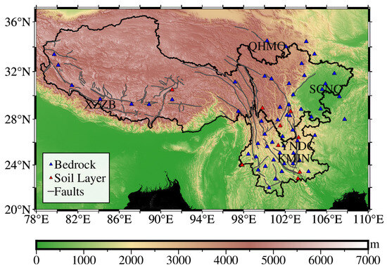
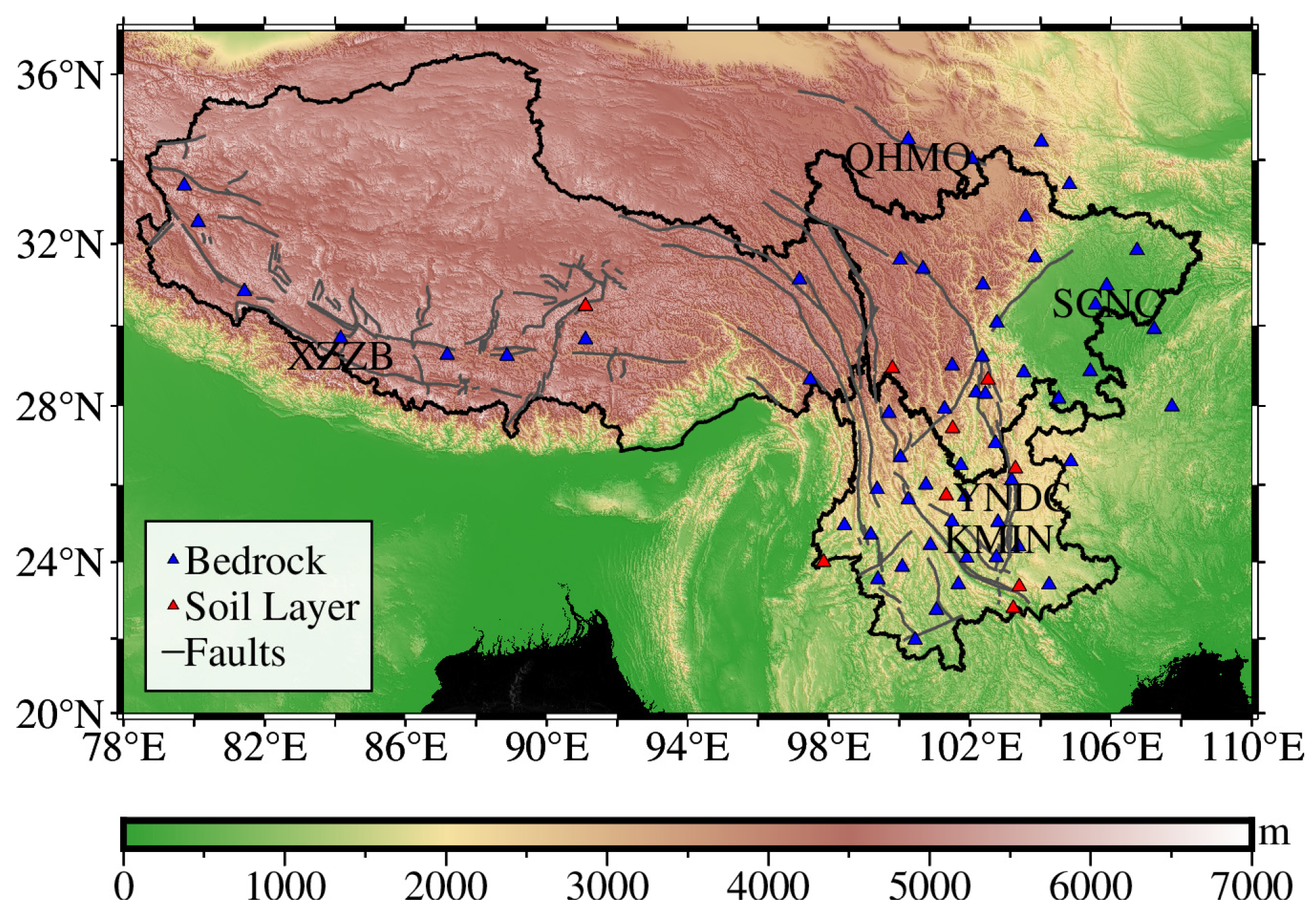
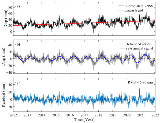
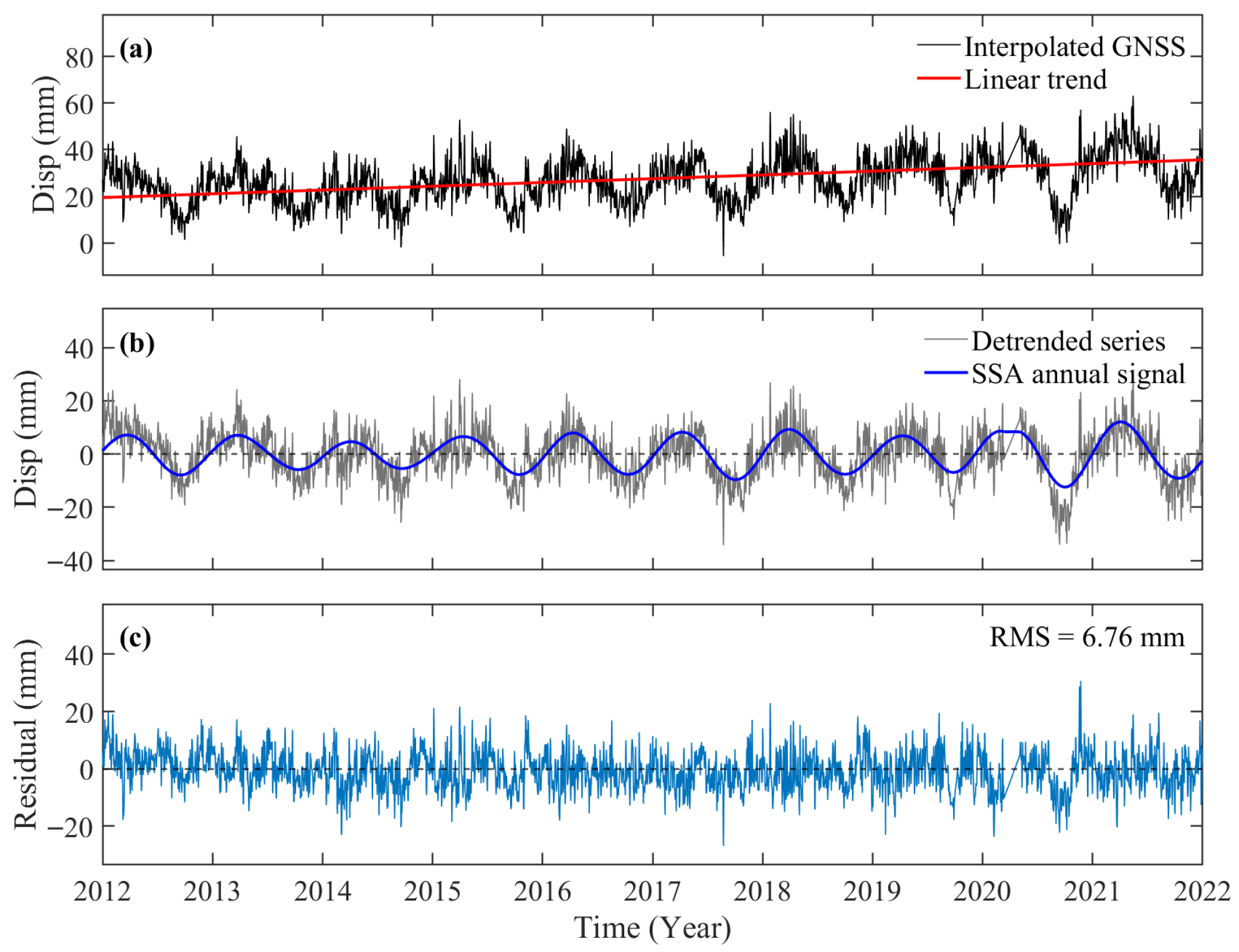
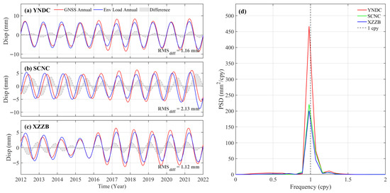
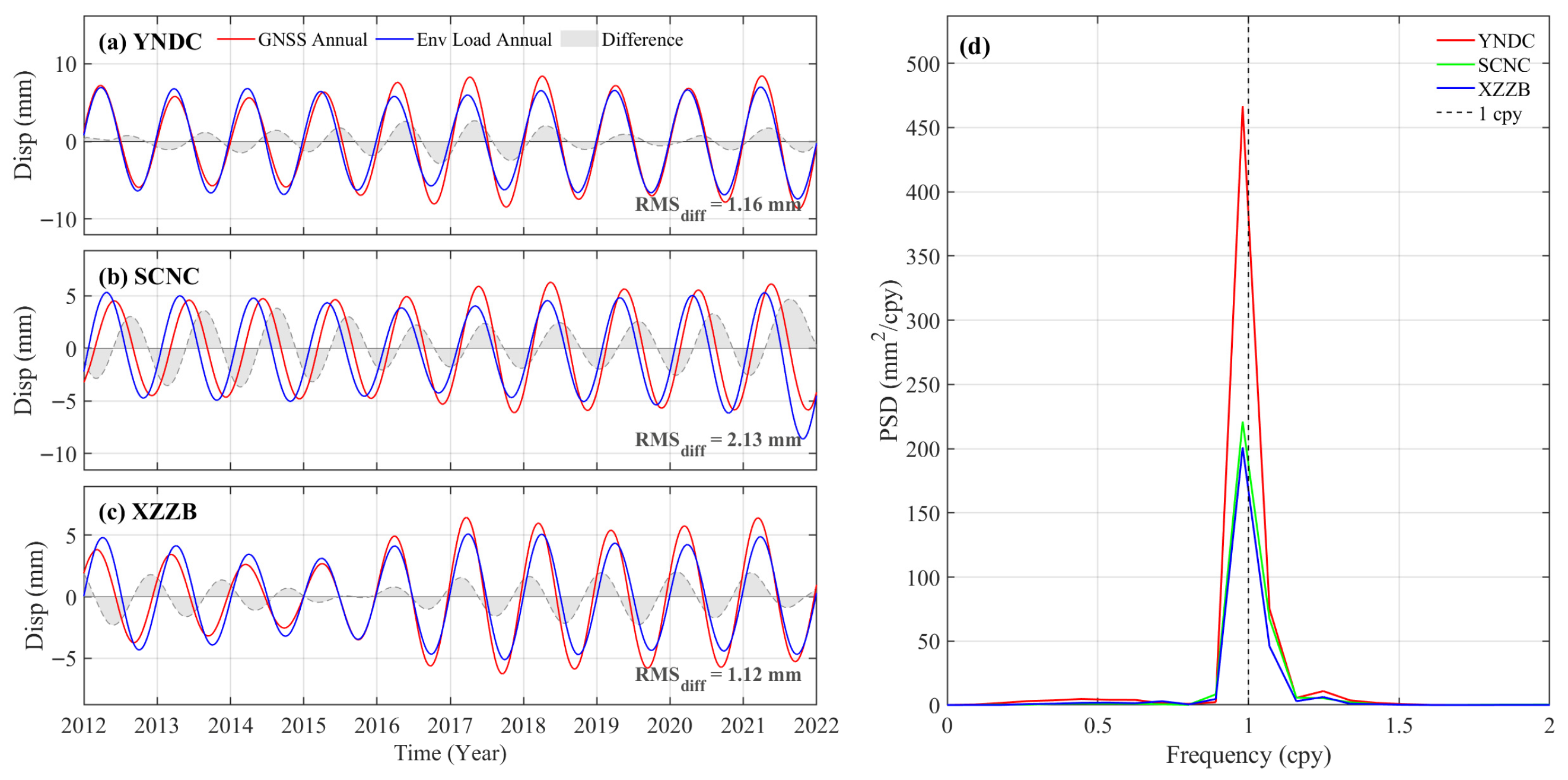
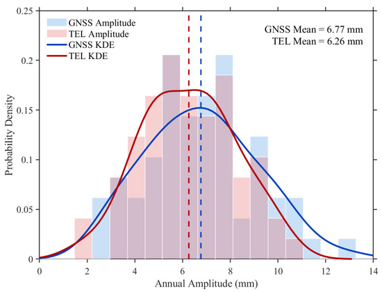
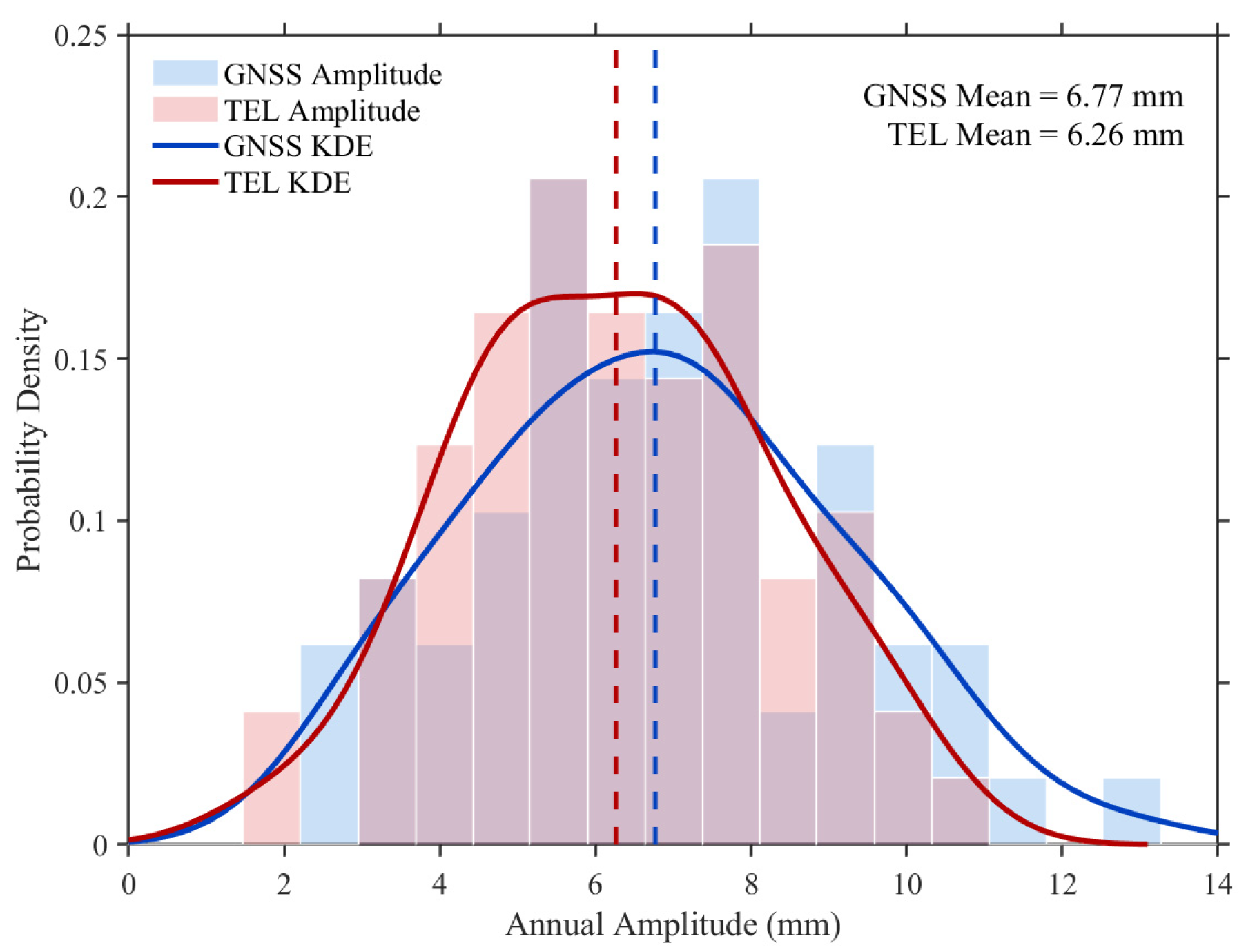
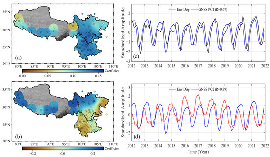
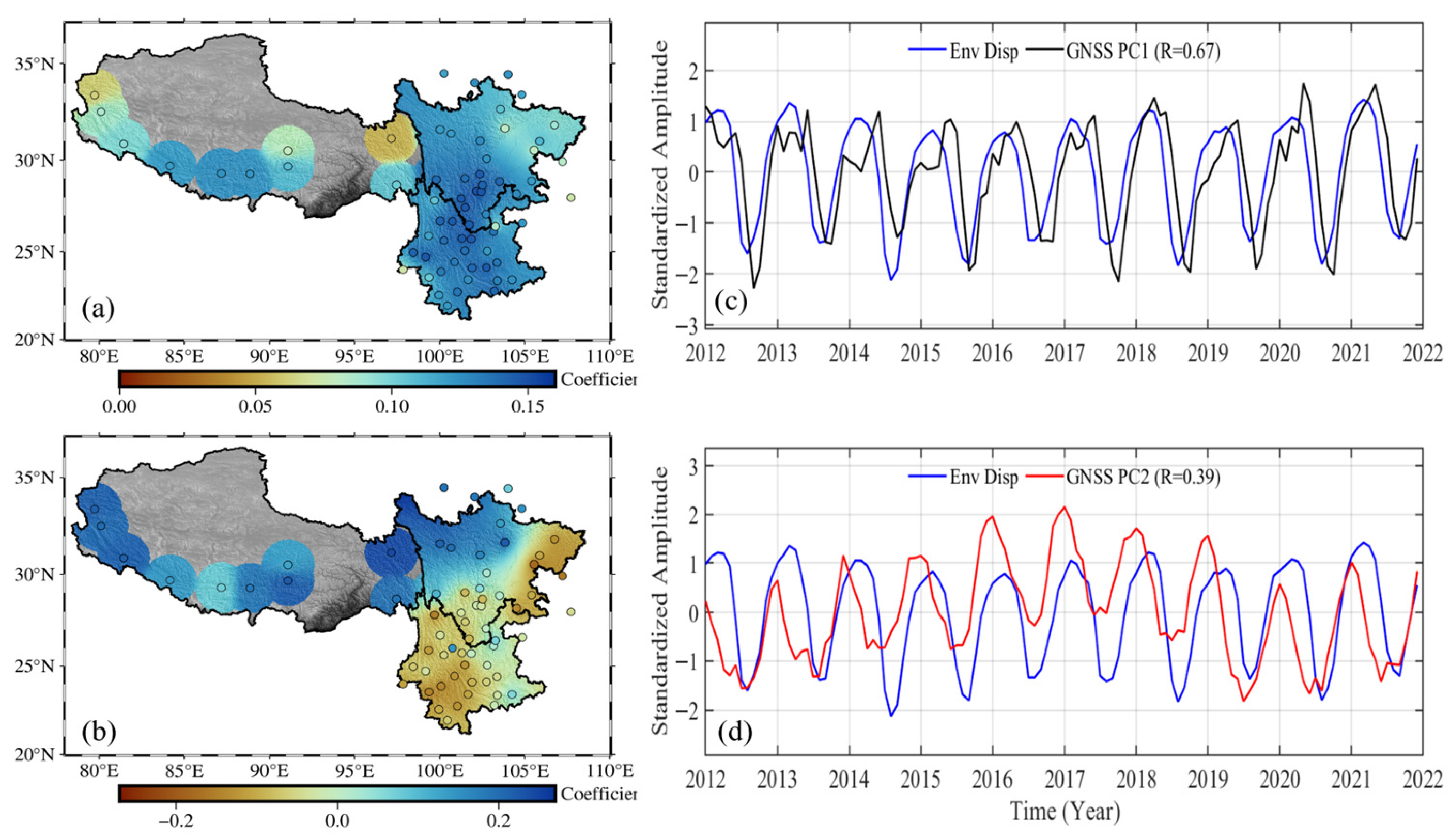
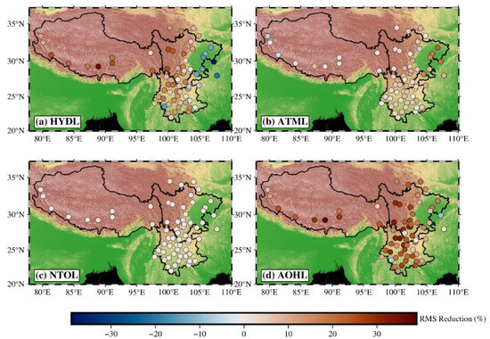
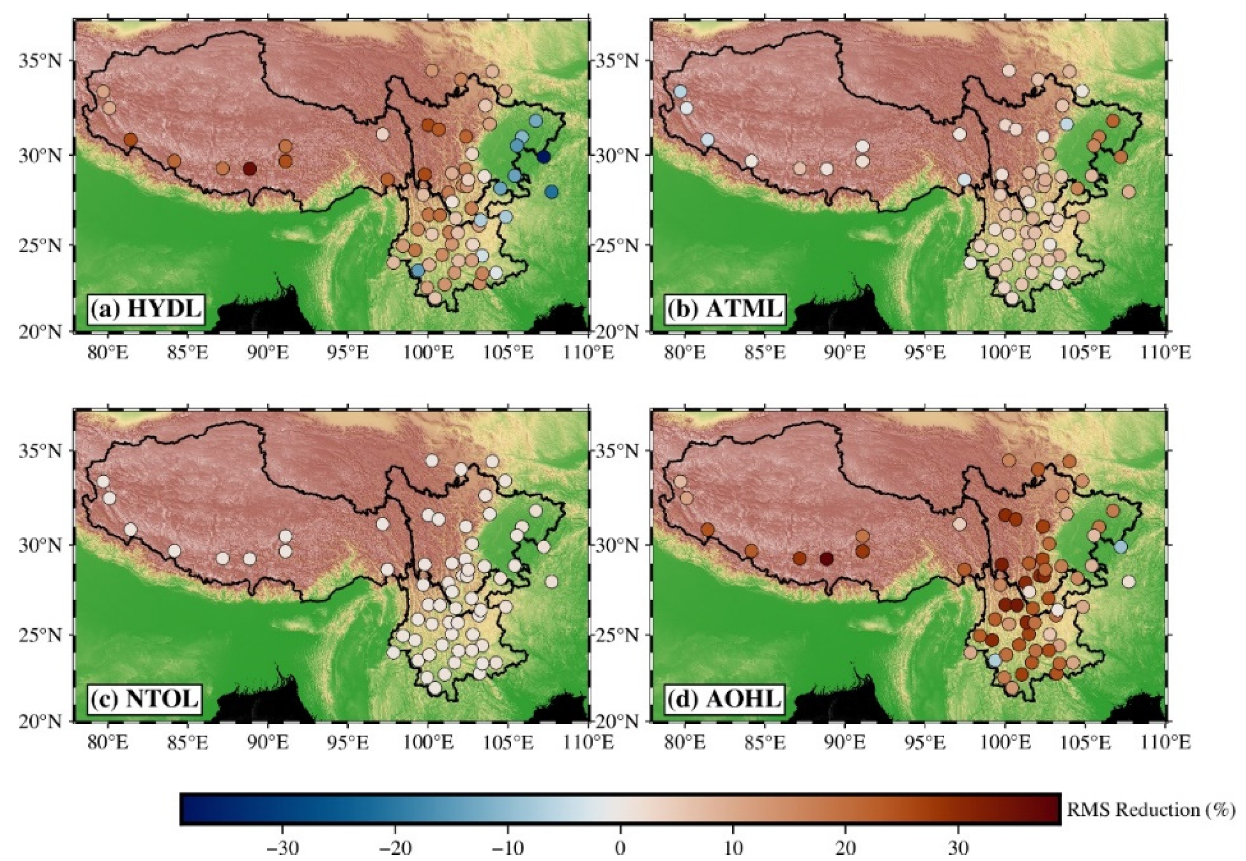
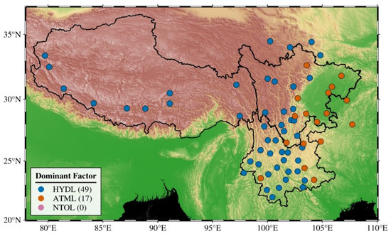
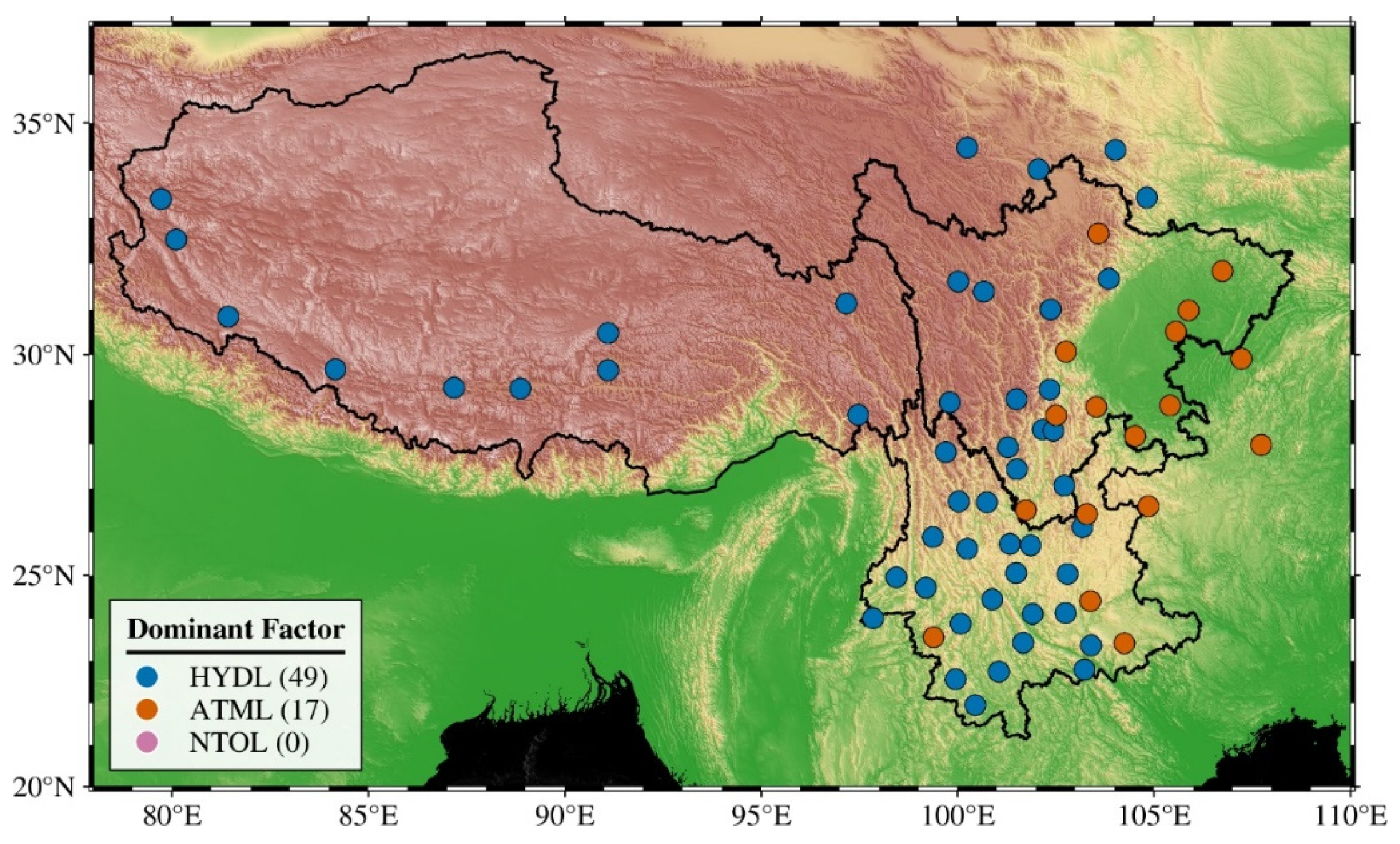
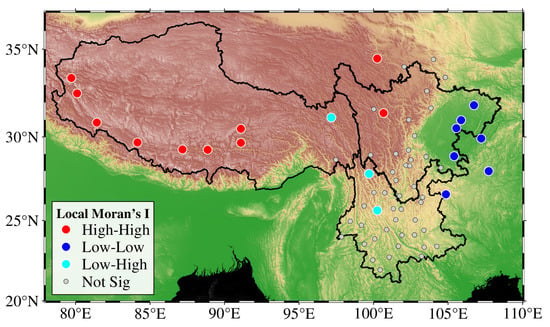
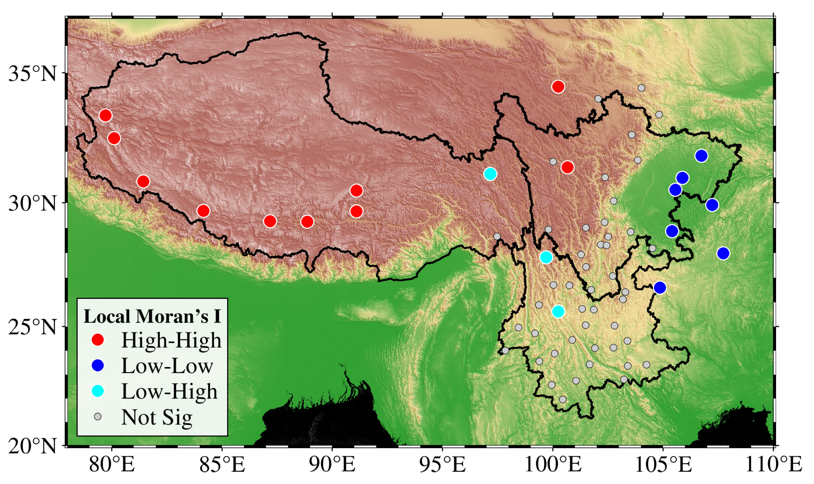
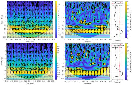
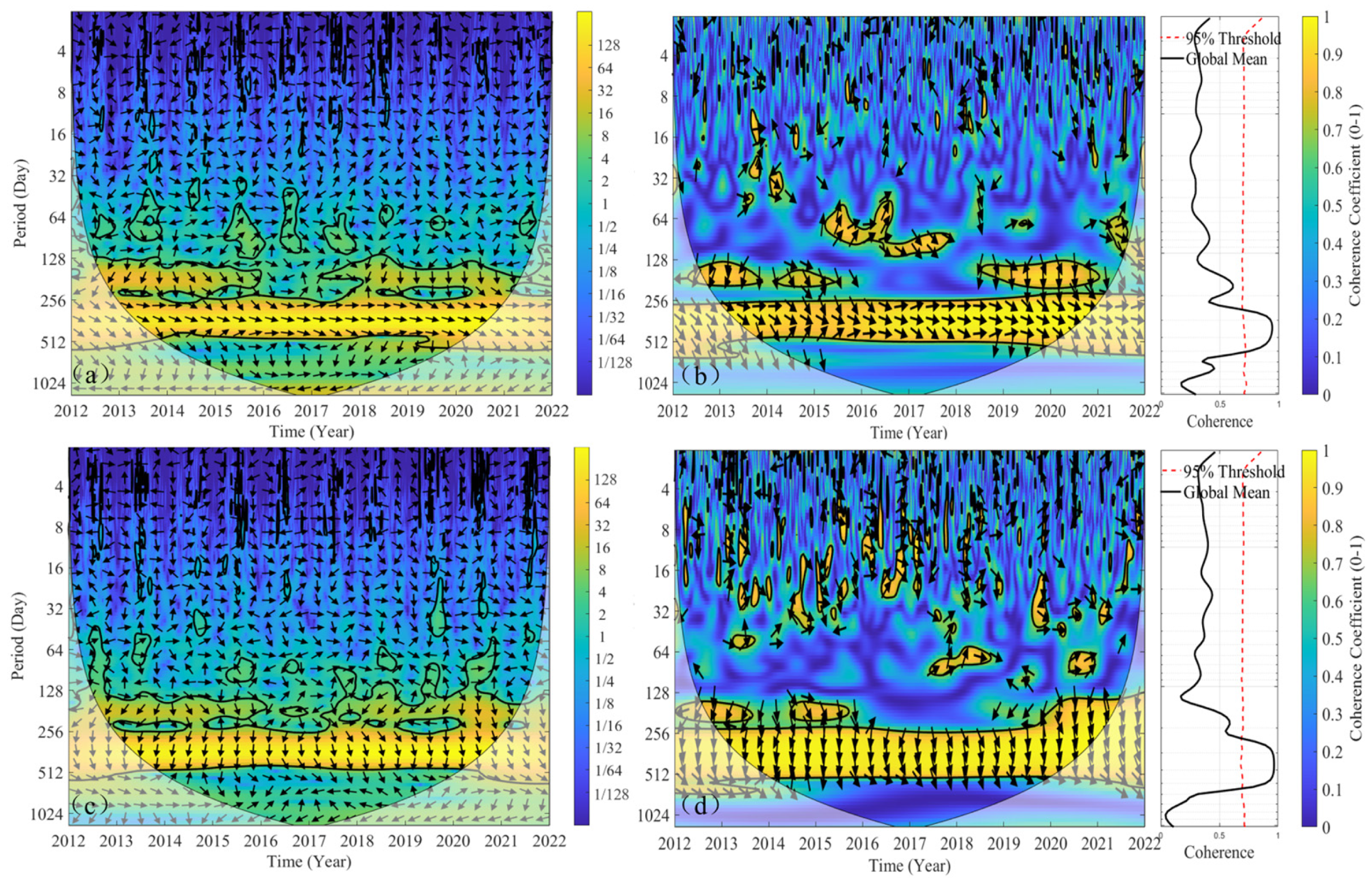
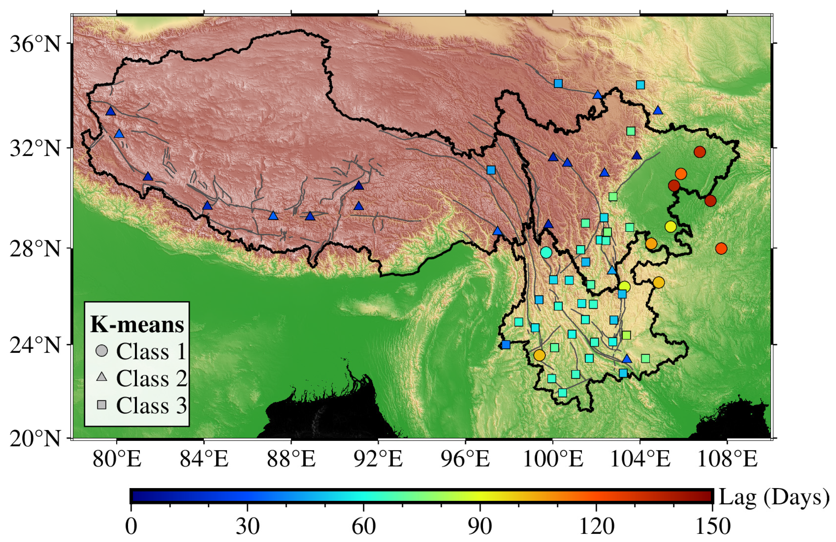
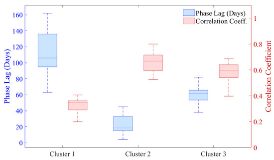
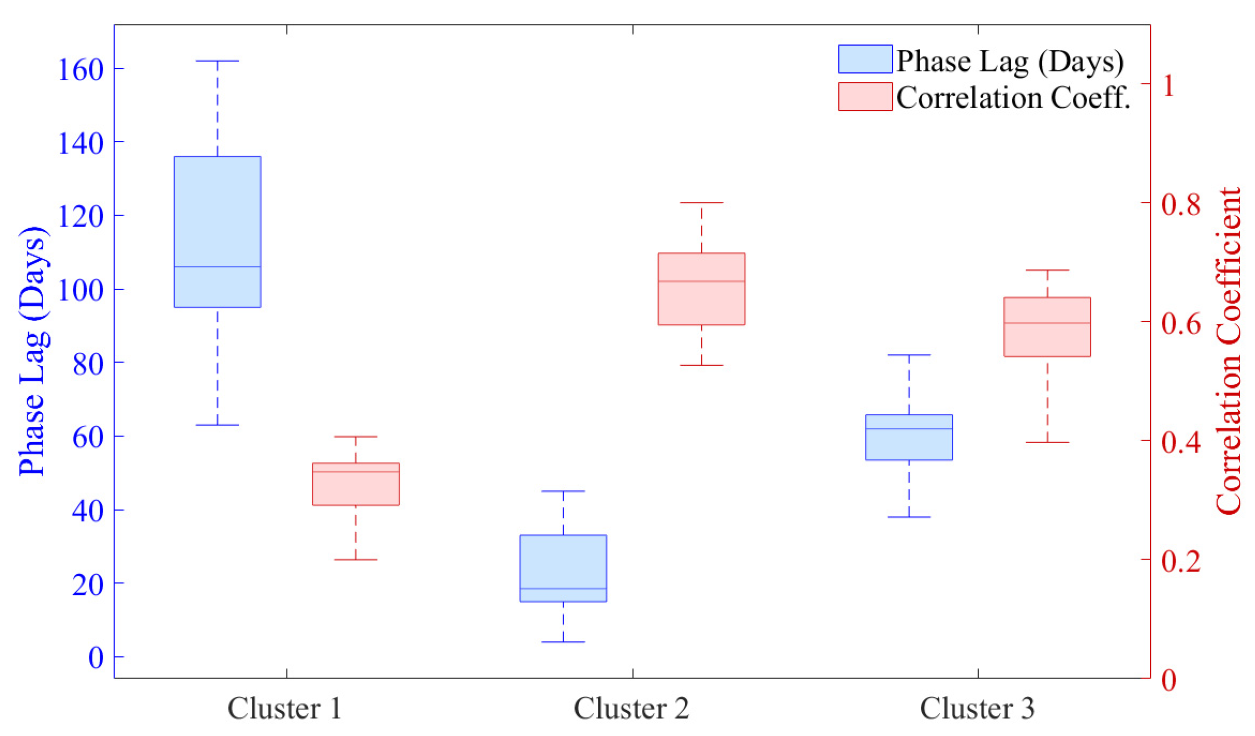

Disclaimer/Publisher’s Note: The statements, opinions and data contained in all publications are solely those of the individual author(s) and contributor(s) and not of MDPI and/or the editor(s). MDPI and/or the editor(s) disclaim responsibility for any injury to people or property resulting from any ideas, methods, instructions or products referred to in the content. |
© 2026 by the authors. Licensee MDPI, Basel, Switzerland. This article is an open access article distributed under the terms and conditions of the Creative Commons Attribution (CC BY) license.