FALB: A Frequency-Aware Lightweight Bottleneck with Learnable Wavelet Fusion and Contextual Attention for Enhanced Ship Classification in Remote Sensing

Highlights

What are the main findings?

• We introduce FALB, a lightweight bottleneck that integrates adaptive wavelet-based frequency filtering with contextual attention to enhance fine-grained ship classification in remote sensing imagery.
• FALB achieves 97.88% accuracy on FGSCM-52, surpassing ResNet-50 by 0.96% and outperforming compared general-purpose baselines while reducing parameters by 30.4%, demonstrating superior efficiency–accuracy trade-offs.

What are the implications of the main findings?

• The frequency-aware design effectively suppresses background noise in complex maritime scenes, enabling more accurate ship type discrimination for real-world surveillance applications.
• FALB’s plug-and-play architecture can be readily integrated into existing CNNbackbones, offering a practical solution for resource-constrained maritime monitoring systems.

Abstract

Ship classification in optical remote sensing requires balancing discriminative representation and model efficiency. Standard convolutional neural network (CNN) bottlenecks rely on local spatial kernels and may emphasize high-frequency texture cues, while stronger backbones increase parameter cost. We propose a frequency-aware lightweight bottleneck (FALB) that couples enhanced wavelet convolution (WTsConv) and contextual anchor attention (CAA) in a cascaded design. WTsConv adopts Sym4 wavelets and a learnable symmetric fusion weight between spatial and wavelet-reconstructed features to improve frequency-aware feature mixing. CAA is then applied to the refined features for contextual aggregation. Integrated into ResNet-50 bottlenecks, FALB is evaluated on FGSCM-52 and achieves 97.88% top-1 accuracy with 17.78 M parameters, compared with 96.92% and 25.56 M for the ResNet-50 baseline, surpassing ResNet-50 by 0.96% and outperforming compared general-purpose baselines while reducing parameters by 30.4%. Under this experimental setting, FALB improves the observed accuracy–parameter trade-off for remote sensing ship classification.

1. Introduction

The rapid advancement of remote sensing technology has enabled ultra-high-resolution satellite imagery, creating opportunities and challenges for maritime ship classification. Although deep learning methods, particularly convolutional neural networks (CNNs) [1], have demonstrated remarkable success, current models [2,3,4,5] still confront two critical limitations when dealing with complex remote sensing scenarios. First, the inherent local receptive field of traditional convolutional kernels restricts their ability to capture global features and low-frequency information, leading to overfitting of high-frequency details (e.g., hull contours) while insufficiently modeling global characteristics (e.g., overall hull distribution). Second, maintaining accuracy with increasing image resolution necessitates deeper models, resulting in rapid parameter growth.

Recent backbone evolution has improved representation quality and training stability, spanning residual and densely connected networks [6,7], inception-style factorized designs [8,9], width/cardinality scaling strategies [10,11], and mobile-efficient families [12,13,14,15,16,17]. However, most of these designs remain primarily spatial-domain operators. As discussed in effective receptive-field analysis [18], nominal kernel size does not directly guarantee robust global context modeling. In practical remote sensing scenes, this may manifest as sensitivity to cluttered local textures and unstable responses under scale and orientation changes.

In parallel, attention-centric and token-based backbones improve long-range modeling ability [19,20,21,22], but their parameter and memory demands can be restrictive for many remote sensing deployment settings. Multi-scale fusion and channel reweighting strategies (e.g., pyramid aggregation and channel recalibration) partially mitigate this gap [23,24], yet explicit frequency-aware modeling is still comparatively limited in lightweight ship classification pipelines.

This challenge is particularly relevant in fine-grained maritime recognition, where class differences can be subtle while background interference is strong. Remote sensing studies and benchmarks have repeatedly shown that complex imaging conditions (viewpoint, scale, sea clutter, harbor structures) significantly affect representation robustness [25,26,27,28,29]. Motivated by these observations, we focus on combining lightweight convolutional design with explicit frequency refinement and context aggregation in a unified bottleneck.

Recent wavelet-based designs such as WTConv [30] expand receptive fields through frequency decomposition but commonly rely on Haar wavelets. For fine-grained ship classification, where hull boundaries and deck structures often vary smoothly, Haar’s first-order vanishing moments may limit smooth-structure representation. This can make it harder to separate global structural cues from high-frequency background textures. In parallel, attention modules applied directly to raw spatial features may over-respond to cluttered sea and dock regions.

To address these issues, we propose a frequency-aware lightweight bottleneck named FALB. We extend WTConv [30] to WTsConv by using the Sym4 basis and a learnable hybrid-scale fusion between spatial and wavelet-reconstructed features. We then place contextual anchor attention (CAA) [31] after WTsConv in a cascaded pipeline, so contextual aggregation is performed on frequency-refined features. This “Frequency-Conditioning followed by Context-Aggregation” design targets a better balance between compactness and representation quality in remote sensing ship classification.

In summary, our main contributions are as follows:

• We propose FALB, a cascaded frequency-spatial bottleneck that combines WTsConv and CAA within ResNet-50 bottlenecks. On FGSCM-52 under our experimental setting, it improves top-1 accuracy by 0.96% while reducing parameters by 30.4% relative to ResNet-50.
• We develop WTsConv with a Sym4 wavelet basis and a learnable hybrid-scale fusion mechanism to mix spatial and wavelet-domain features inside the convolution block.
• We design a cascaded ordering of WTsConv and CAA and analyze its effect through ablation and visualization to show how frequency refinement and contextual attention interact.

2. Related Work

2.1. Ship Classification in Optical Remote Sensing

The rapid development of high-resolution satellite imagery has propelled maritime ship classification from traditional methods to deep learning-based approaches [27]. Fine-grained ship classification datasets, such as FGSCR-42 [32] and FGSCM-52 [29], have driven innovations in multi-scale feature representation [28]. Recent advances have also explored large vision-language models and prompt tuning [29] to address data scarcity, albeit at substantial computational costs. Despite these advances, separating intrinsic hull structures from complex ocean clutter remains challenging. Explicit multi-frequency modeling—decoupling low-frequency structural cues from high-frequency texture and noise—is comparatively less studied in fine-grained ship recognition.

Beyond ship-specific benchmarks, broader remote sensing scene and aerial-object studies also indicate that appearance variation across scale, orientation, and acquisition condition is a key source of performance instability [25,26]. This has motivated stronger feature pyramids, context aggregation, and cross-scale fusion in downstream maritime tasks. Nevertheless, many existing methods still rely on purely spatial feature processing, so background texture suppression and structural cue preservation are not explicitly disentangled in the spectral sense.

Furthermore, considering that remote sensing ship classification often faces severe challenges such as limited labeled samples and subtle inter-class differences, purely architectural improvements are sometimes insufficient. Recent paradigms utilizing semi-supervised learning and collaborative learning—such as theoretically justified frameworks extending from mutual guide to Confucius tri-learning [33]—provide crucial complementary strategies to architectural designs, offering promising pathways for mitigating label scarcity in fine-grained maritime recognition.

2.2. Lightweight CNNs

To address the parameter explosion problem in deep networks, lightweight CNN architectures have been extensively developed. Early compact models such as SqueezeNet [12] and MobileNet [34] focused on replacing expensive dense convolutions. Subsequent designs, including MobileNetV2/V3 [13,15], ShuffleNet/ShuffleNetV2 [14,35], GhostNet [36], and EfficientNet/EfficientNetV2 [16,17], further improved the accuracy–efficiency trade-off through inverted bottlenecks, channel shuffling, cheap feature generation, and compound scaling.

In the broader CNN literature, width and cardinality scaling (e.g., Wide-ResNet and ResNeXt) demonstrate that representational diversity can be improved without naively increasing depth [10,11]. However, these optimizations are still mostly spatial-domain in nature. In remote sensing ship imagery, purely spatial lightweight designs may remain sensitive to background high-frequency textures and geometric clutter, motivating explicit spectral refinement inside compact bottlenecks.

However, conventional lightweight CNNs primarily optimize FLOPs and parameter counts through architectural modifications in the spatial domain, often treating high-frequency and low-frequency information uniformly. In remote sensing ship imagery, this may increase sensitivity to high-frequency textures (e.g., background waves and docks) while weakening global structural modeling (e.g., overall hull layout). This observation motivates adding explicit frequency-aware processing to lightweight bottlenecks.

2.3. Frequency-Domain and Wavelet-Based Deep Models

The wavelet transform provides a natural multi-scale analysis framework by decomposing signals into components of different frequencies. Its theoretical foundation is well established in multiresolution analysis [37,38], and wavelet-inspired deep representations have shown strong invariance and stability properties in vision tasks [39]. Several recent works have further explored integrating wavelets with deep learning for remote sensing and image processing [40,41]. For instance, FcaNet [42] introduced the discrete Cosine transform (DCT) into channel attention to demonstrate the value of frequency-domain processing.

Notably, Li et al. [43] proposed WaveCNet, which processes features through physically separated high-frequency and low-frequency subband branches, combining them via learnable weights at the end. This branch-separated strategy is effective, but it may weaken early interaction between spatial-domain and frequency-domain cues. In our design, a learnable hybrid-scale fusion mechanism performs symmetric fusion of raw spatial features and wavelet-reconstructed features within the convolution block, enabling tighter coupling during feature extraction.

Furthermore, to address the inherent limitation of small receptive fields in traditional convolutions, Finder et al. [30] proposed WTConv. WTConv expands the effective receptive field using wavelet decomposition, but it mainly uses Haar wavelets. Haar is computationally simple, yet for ship imagery with smooth structural transitions, higher-order bases may provide richer representation. Our WTsConv therefore adopts Sym4 wavelets, which have higher-order vanishing moments and are expected to better model smooth hull contours.

2.4. Attention and Context-Aware Modeling in Remote Sensing

Attention mechanisms have proven effective for capturing long-range dependencies and contextual information in remote sensing tasks. From non-local interaction [44] and global-context refinement [45] to efficient channel calibration [46] and criss-cross spatial modeling [47], attention modules provide a broad design space for context-aware feature enhancement. Architectures like Transformers [48], DeiT [20], PVT [22], CBAM [49], and DANet [50] dynamically assign weights to achieve global receptive fields and robust contextual modeling.

However, existing attention mechanisms primarily operate in the spatial domain without explicit constraints on frequency distribution. Applying attention directly to raw spatial features in maritime scenes may increase sensitivity to cluttered high-frequency background responses [51,52]. Combining frequency-domain refinement with spatial attention in an ordered pipeline is still relatively less explored.

Our FALB follows a “Frequency-Conditioning followed by Context-Aggregation” pipeline. By positioning WTsConv before the contextual anchor attention (CAA) module, frequency refinement is performed prior to attention-based context modeling. This ordering is intended to reduce background interference before receptive-field expansion, and its impact is further analyzed in our ablation study.

2.5. Synthesis of Research Gap

The above literature indicates that current progress can be organized into three largely independent optimization directions: compact spatial architecture design, context modeling by attention/token interaction, and explicit frequency decomposition. Compact CNNs and re-parameterization-based models improve deployment efficiency [13,15,16,17,34,53]. Transformer and MLP-like paradigms strengthen long-range dependency modeling [19,20,21,22,54,55]. Frequency-domain methods provide additional robustness against texture bias [30,42,43]. Yet, these lines are often explored separately, and their coupling strategy is usually not the central design target.

For fine-grained ship classification, the practical challenge is not only to improve accuracy but to improve the accuracy–parameter trade-off under severe background clutter. In this context, a key unresolved question is how to build a lightweight bottleneck where frequency refinement and context aggregation are explicitly ordered and tightly coupled, instead of being attached as loosely connected modules. Table 1 summarizes representative families and their remaining gaps in relation to this objective.

Table 1. Concise summary of representative families and remaining gaps for fine-grained ship classification.

Family	Representative Works	Key Remaining Gap in Ship Classification
Spatial CNN backbones	ResNet, DenseNet, Xception, ConvNeXt, RepVGG [4,5,6,7,53]	Limited explicit frequency control under sea/dock clutter.
Mobile/lightweight CNNs	MobileNet series, ShuffleNet series, GhostNet, EfficientNet family [13,14,15,16,17,34,35,36]	Efficiency gains can come with weaker global structural cues in cluttered maritime backgrounds.
Attention and token-based models	Non-local/GC/ECA/CC attention, ViT/DeiT/PVT/Swin/PiT/ResMLP [19,20,21,22,44,45,46,47,54,55]	Attention on raw spatial features can still amplify irrelevant high-frequency background responses.
Frequency-aware designs	FcaNet, WaveCNet, WTConv, recent wavelet-enhanced remote sensing models [30,40,41,42,43]	The ordering between frequency refinement and context aggregation is often underexplored in lightweight bottlenecks.
Remote sensing ship-oriented methods	Feature-fusion and prompt-tuning pipelines with dedicated benchmarks [27,28,29,32,56]	Limited unified analysis of frequency-aware lightweight bottleneck design under strict complexity constraints.

3. Method

3.1. Overview: Cascaded Architecture

FALB is a frequency-aware lightweight bottleneck designed to improve the accuracy–parameter balance for remote sensing ship classification. Its forward path follows two stages: Frequency-Conditioning and Context-Aggregation.

In each modified ResNet50 bottleneck, the original spatial convolution is replaced with WTsConv, and CAA is applied afterward. WTsConv performs wavelet-based frequency refinement and learnable fusion between spatial and wavelet-reconstructed features. CAA then predicts an attention map from the refined feature and applies residual modulation. With this ordering, contextual attention operates on frequency-conditioned representations rather than directly on raw spatial responses.

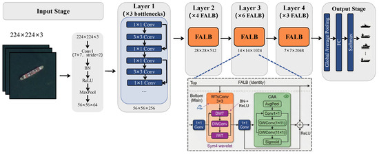
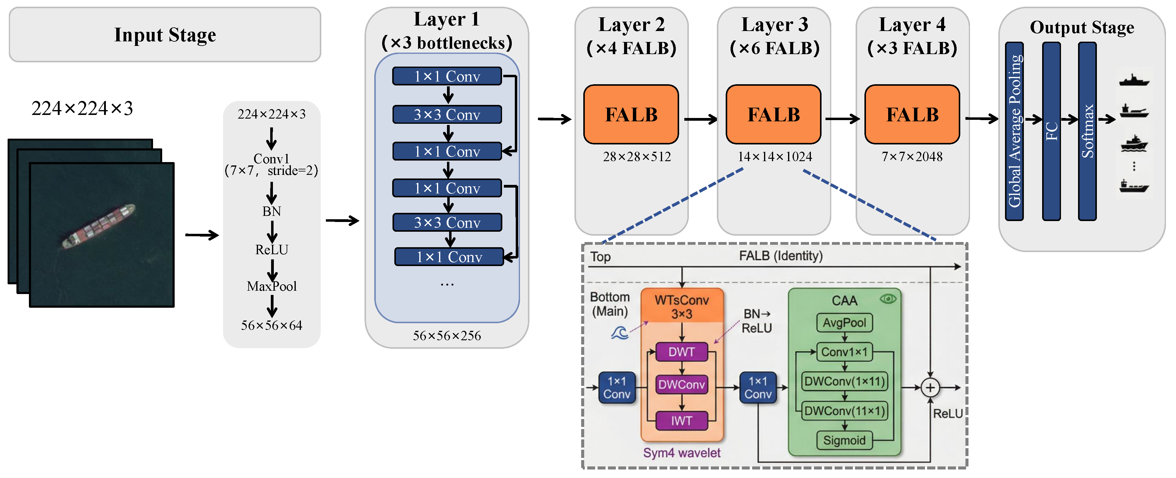
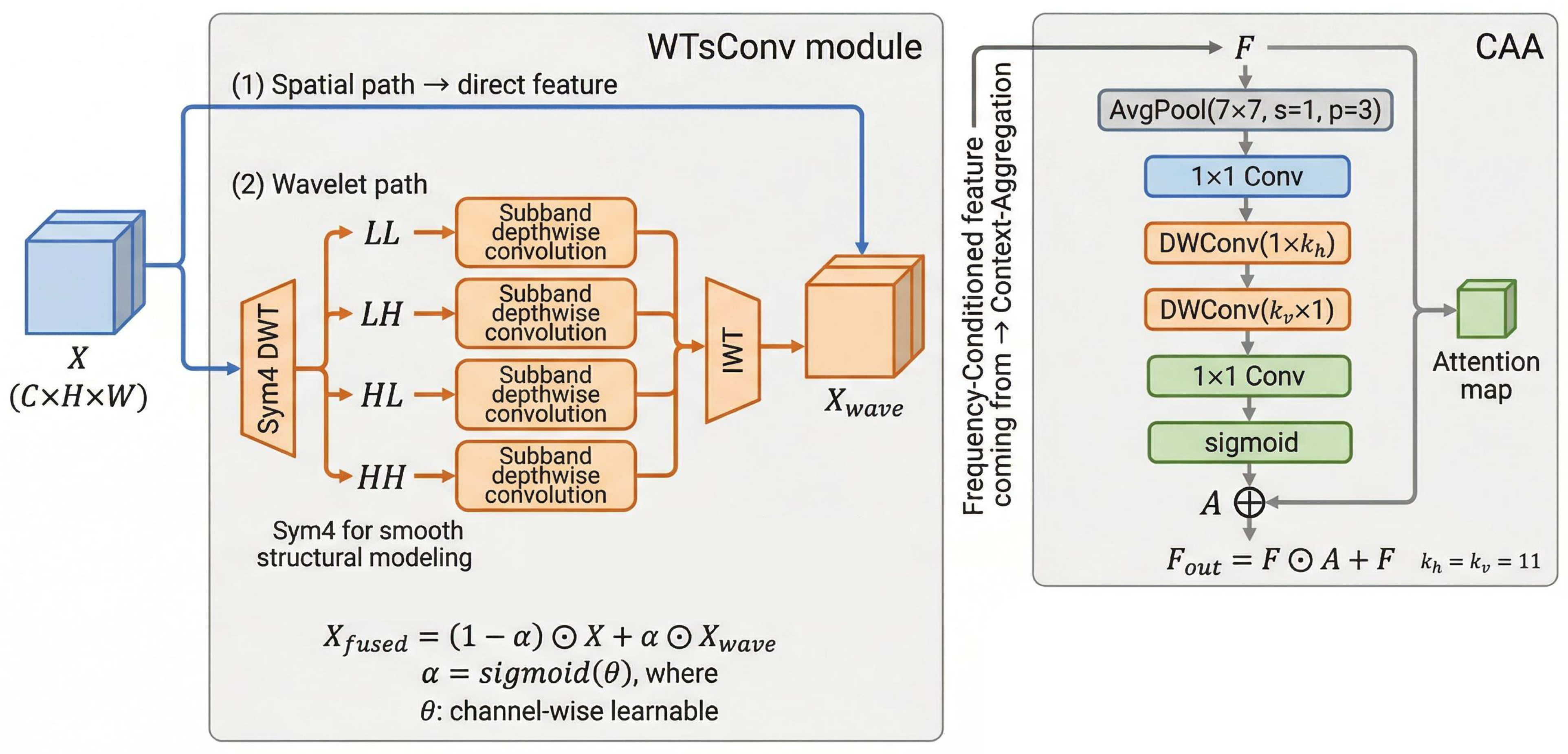
Algorithm 1 provides the block-level forward process used in this work. The backbone-level integration of FALB is illustrated in Figure 1, the internal structure of WTsConv is shown in Figure 2, and quantitative/visualization comparisons are provided in Figure 3.

Algorithm 1 Forward pass of the proposed FALB module.

Require: Input feature map ${\mathbf{X}}_{in}\in {\mathbb{R}}^{C_{in}\times H\times W}$ Ensure: Output feature map ${\mathbf{X}}_{out}\in {\mathbb{R}}^{C_{out}\times H^{\prime }\times W^{\prime }}$ 1: ${\mathbf{X}}_{id}\leftarrow {\mathbf{X}}_{in}$                           // Identity branch 2: ${\mathbf{X}}_1\leftarrow \mathrm{ReLU}\left(\mathrm{BN}\left({\mathrm{Conv}}_{1\times 1}\left({\mathbf{X}}_{in}\right)\right)\right)$ 3: // Stage 1: Frequency-Conditioning (conv2) 4: ${\mathbf{X}}_2\leftarrow \mathrm{DWSP}\_\mathrm{WTsConv}\left({\mathbf{X}}_1\right)$      // Depthwise WTsConv + pointwise conv 5: ${\mathbf{X}}_2\leftarrow \mathrm{ReLU}\left(\mathrm{BN}\left({\mathbf{X}}_2\right)\right)$ 6: // Stage 2: Context-Aggregation via CAA 7: ${\mathbf{X}}_3\leftarrow \mathrm{BN}\left({\mathrm{Conv}}_{1\times 1}\left({\mathbf{X}}_2\right)\right)$ 8: $\mathbf{A}\leftarrow \mathrm{CAA}\left({\mathbf{X}}_3\right)$ 9: ${\mathbf{X}}_{att}\leftarrow {\mathbf{X}}_3\odot \mathbf{A}+{\mathbf{X}}_3$ 10: if downsample exists then 11:    ${\mathbf{X}}_{id}\leftarrow \mathrm{Downsample}\left({\mathbf{X}}_{id}\right)$ 12: end if 13: ${\mathbf{X}}_{out}\leftarrow \mathrm{ReLU}({\mathbf{X}}_{att}+{\mathbf{X}}_{id})$ 14: return${\mathbf{X}}_{out}$

Figure 1. Overview of FALB integration into ResNet50. Bottlenecks in Layer 1 ($\times 3$) remain unchanged, while bottlenecks in Layers 2–4 ($\times 4,\times 6,\times 3$) are replaced by the proposed FALB bottleneck. The lower panel shows the cascaded path $1\times 1$ Conv → WTsConv → BN/ReLU →$1\times 1$ Conv → CAA, followed by identity addition (with downsample when needed) and ReLU. The CAA block applies residual modulation as defined in Equation (7). For schematic clarity, tensor sizes are shown in a simplified form.

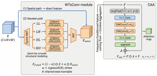
Figure 2. Detailed architecture of the proposed WTsConv module and CAA mechanism. Left (WTsConv): The input feature $\mathbf{X}\in {\mathbb{R}}^{C\times H\times W}$ follows two parallel paths: (1) a direct spatial path preserving original features, and (2) a wavelet path performing Sym4-based DWT decomposition into four subbands (LL: low-low frequency, LH: low–high frequency, HL: high–low frequency, HH: high–high frequency), followed by subband-wise depthwise convolutions and IWT reconstruction to obtain ${\mathbf{X}}_{wave}$. The two paths are fused via a learnable channel-wise weight $\alpha =\sigma \left(\mathit{\theta }\right)$ to produce ${\mathbf{X}}_{fused}=(1-\alpha )\odot \mathbf{X}+\alpha \odot {\mathbf{X}}_{wave}$, where ⊙ denotes element-wise multiplication. Right (CAA): The contextual anchor attention module takes the frequency-conditioned feature $\mathbf{F}$ as input, applies average pooling ($7\times 7$, stride = 1, padding = 3), followed by two $1\times 1$ convolutions and two directional depthwise convolutions ($k_h\times 1$ and $1\times k_v$, where $k_h=k_v=11$) to generate the attention map $\mathbf{A}$. The output applies residual modulation: ${\mathbf{F}}_{out}=\mathbf{F}\odot \mathbf{A}+\mathbf{F}$. This cascaded design enables frequency-aware feature refinement followed by context-aware attention aggregation.

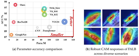
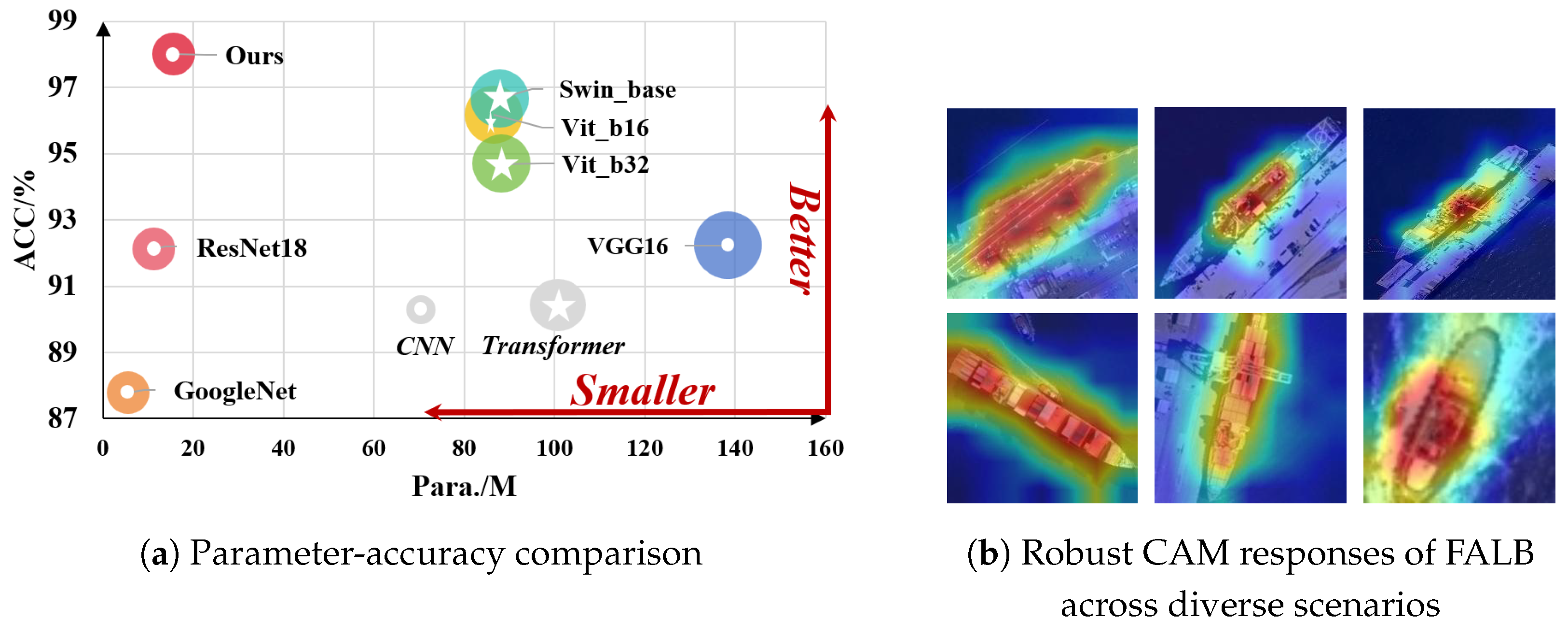
Figure 3. Comparison of parameter-accuracy trade-off and attention robustness: (a) FALB improves accuracy by 0.96% over ResNet50 while reducing parameters by 30.4% under the reported setting, achieving the optimal balance among compared baselines; (b) Grad-CAM visualizations of FALB across diverse and challenging maritime scenarios (including massive aircraft carriers, severe port clutter with gantry cranes, and intense high-speed wave wakes). The highly concentrated responses explicitly demonstrate that FALB consistently localizes intrinsic ship structures and effectively suppresses severe high-frequency background noise.

3.2. WTsConv: Enhanced Wavelet Convolution

We enhance WTConv [30] with two key modifications to form WTsConv (Figure 2). First, we replace Haar wavelets (which possess only first-order vanishing moments) with Sym4 wavelets. Haar wavelets accurately represent constant signals but fail to capture the smooth gradient variations inherent in complex ship hull contours. Sym4 wavelets overcome this by possessing fourth-order vanishing moments:

$${\int }_{-\infty }^{\infty }{t}^k{\psi }_{\mathrm{Sym}4}\left(t\right)dt=0\mathrm{for}k=0,1,2,3.$$

(1)

Here, t denotes the spatial variable, k represents the order of the vanishing moment, and ${\psi }_{\mathrm{Sym}4}\left(t\right)$ is the Sym4 mother wavelet function. These higher vanishing moments enable the precise representation of cubic polynomial signals, better modeling the gradual structural transitions in remote sensing data and significantly reducing high-frequency noise leakage into low-frequency subbands. While adopting the Sym4 basis increases the filter length compared to Haar, introducing a slight parameter overhead (+0.76 M), it significantly enhances the modeling capability for smooth structural transitions.

Second, existing methods often process frequency subbands in separate parallel branches, which can weaken early interaction between spatial and frequency cues. To improve coupling, we use a learnable hybrid-scale fusion mechanism inside WTsConv. Let $\mathbf{X}\in {\mathbb{R}}^{C\times H\times W}$ be the input feature map to the WTs depthwise branch (where C is the number of channels, and H and W are the spatial height and width). The wavelet-domain operation is defined as:

$${\mathbf{X}}_{wave}=\mathrm{IWT}\left(\mathrm{DWConv}\left(\mathrm{DWT}\left(\mathbf{X}\right)\right)\right),$$

(2)

where $\mathrm{DWT}$ and $\mathrm{IWT}$ denote the discrete wavelet transform and inverse wavelet transform respectively, $\mathrm{DWConv}$ represents the depthwise convolution applied to the decomposed subbands, and ${\mathbf{X}}_{wave}\in {\mathbb{R}}^{C\times H\times W}$ is the reconstructed feature map from the frequency domain.

In the default sym fusion mode used in our main experiments, the fusion weight is a learnable channel-wise parameter:

$$\alpha =\sigma \left(\mathit{\theta }\right),\mathit{\theta }\in {\mathbb{R}}^{C\times 1\times 1},$$

(3)

where $\theta$ is the learnable parameter vector, $\sigma (·)$ represents the Sigmoid activation function to constrain the weights to $(0,1)$, and $\alpha \in {\mathbb{R}}^{C\times 1\times 1}$ is the resulting channel-wise scaling factor. The fused feature map ${\mathbf{X}}_{\mathrm{fused}}\in {\mathbb{R}}^{C\times H\times W}$ is then calculated as

$${\mathbf{X}}_{\mathrm{fused}}=(1-\alpha )\odot \mathbf{X}+\alpha \odot {\mathbf{X}}_{wave},$$

(4)

where ⊙ denotes element-wise multiplication with channel broadcasting. This learnable mechanism balances spatial detail retention and frequency-domain refinement with very small parameter overhead.

Design rationale for channel-wise fusion. While more adaptive fusion strategies (e.g., spatial-dependent gates or region-conditioned weights) could potentially better handle heterogeneous ship regions (hull vs. superstructure), we adopt channel-wise symmetric fusion as the default design in this study for deployment-oriented considerations: (1) parameter efficiency—symmetric fusion introduces only C learnable parameters per bottleneck; (2) computational simplicity—it does not require an additional dynamic gating branch; (3) training stability—the multi-seed results in Section 4.4 suggest lower variance than the decoupled alternative; and (4) plug-and-play simplicity—the symmetric design maintains a clean interface for integration into existing ResNet-style architectures. We acknowledge that region-aware adaptive fusion is promising and warrants further investigation in future work.

3.3. Contextual Anchor Attention (CAA)

To address background interference and context aggregation on frequency-refined features, we use the contextual anchor attention (CAA) module [31]. Given the input feature map $\mathbf{F}\in {\mathbb{R}}^{C\times H\times W}$ (corresponding to ${\mathbf{X}}_3$ in Algorithm 1), CAA first applies local average pooling with a spatial kernel size of $7\times 7$, a stride of $s=1$, and padding $p=3$:

$${\mathbf{F}}_p={\mathrm{AvgPool}}_{7\times 7,s=1,p=3}\left(\mathbf{F}\right),$$

(5)

where ${\mathbf{F}}_p\in {\mathbb{R}}^{C\times H\times W}$ is the pooled feature preserving the original dimensions.

Then, CAA computes a 3D attention map using two pointwise convolutions (${\mathrm{Conv}}_{1\times 1}$) and two directional depthwise convolutions ($\mathrm{DWConv}$):

$$\mathbf{A}=\sigma \left({\mathrm{Conv}}_{1\times 1}^{\left(2\right)}\left({\mathrm{DWConv}}_{k_v\times 1}\left({\mathrm{DWConv}}_{1\times k_h}\left({\mathrm{Conv}}_{1\times 1}^{\left(1\right)}\left({\mathbf{F}}_p\right)\right)\right)\right)\right),$$

(6)

where $k_h$ and $k_v$ are the horizontal and vertical kernel sizes (set to $k_h=k_v=11$ in our implementation), and $\sigma (·)$ is the Sigmoid activation function. These operations preserve the spatial size and channel count, yielding the final attention map $\mathbf{A}\in {[0,1]}^{C\times H\times W}$.

The output feature map ${\mathbf{F}}_{\mathrm{out}}$ is computed using residual modulation:

$${\mathbf{F}}_{\mathrm{out}}=\mathbf{F}\odot \mathbf{A}+\mathbf{F},$$

(7)

where ⊙ denotes element-wise multiplication. In FALB, this attention mechanism is applied strictly after WTsConv, ensuring that the contextual reweighting ($\mathbf{F}\odot \mathbf{A}$) is performed on features that have already been frequency-conditioned.

Theoretical rationale for the cascaded design: From a signal-processing perspective, applying spatial attention directly to raw features (which contain a mixture of task-relevant structural signals and high-frequency background clutter) risks amplifying the noise components. By mathematically bounding the frequency spectrum first via WTsConv, the intermediate feature manifold $\mathbf{F}$ is explicitly conditioned to suppress irrelevant high-frequency responses. Consequently, the subsequent contextual anchor attention is theoretically constrained to operate on a refined, low-noise manifold. This prevents the learned attention weights $\mathbf{A}$ from overfitting to local texture artifacts (e.g., sea waves or complex dock structures). Therefore, the “Frequency-Conditioning followed by Context-Aggregation” cascade forms a theoretically sound “filter-then-attend” paradigm, rather than an empirical stacking of sub-modules.

3.4. FALB Architecture Integration

FALB modifies ResNet50’s bottleneck architecture by replacing standard $3\times 3$ convolutions with our designed WTsConv and strictly cascading CAA for subsequent feature refinement (see Figure 1). ResNet50 contains four layers with $\{3,4,6,3\}$ bottlenecks respectively; we replace all bottlenecks except those in the first layer to preserve initial low-level feature integrity.

3.5. Complexity and Deployment Analysis

To clarify the efficiency motivation of FALB, we summarize the parameter and compute characteristics of the bottleneck replacement. For a standard convolution with kernel size k, input channels $C_{in}$, output channels $C_{out}$, and feature size $H\times W$, the parameter count and multiply–accumulate operations (MACs) are

$$P_{\mathrm{std}}=k^2{C}_{in}{C}_{out},{\mathrm{MAC}}_{\mathrm{std}}=HW{k}^2{C}_{in}{C}_{out}.$$

(8)

For depthwise-pointwise decomposition, they become

$$P_{\mathrm{dw}+\mathrm{pw}}=k^2{C}_{in}+C_{in}{C}_{out},{\mathrm{MAC}}_{\mathrm{dw}+\mathrm{pw}}=HW(k^2{C}_{in}+C_{in}{C}_{out}).$$

(9)

The parameter ratio is

$${\rho }_P={\displaystyle \frac{P_{\mathrm{dw}+\mathrm{pw}}}{P_{\mathrm{std}}}}={\displaystyle \frac{1}{C_{out}}}+{\displaystyle \frac{1}{k^2}},$$

(10)

which is typically much smaller than 1 in practical settings.

WTsConv keeps this lightweight depthwise–pointwise backbone and adds a wavelet branch plus channel-wise fusion parameters:

$$P_{\mathrm{WTs}}\approx P_{\mathrm{dw}+\mathrm{pw}}+P_{\mathrm{wave}}+C,$$

(11)

where the C term comes from the learnable fusion vector $\mathit{\theta }\in {\mathbb{R}}^{C\times 1\times 1}$. CAA introduces additional context modeling with directional depthwise operations and $1\times 1$ projections, increasing capacity while preserving the compact bottleneck interface.

Using the reported results in Table 2, we further derive deployment-oriented indicators in Table 3. Here, ACC/M denotes top-1 accuracy divided by parameter count (in millions), and FP32 size is approximated as Params $\times 4$ bytes.

Table 2. Comparison of accuracy and parameter count between FALB and state-of-the-art methods on FGSCM-52 dataset.

Model	Type	Para.	ACC
ResNet18 [6]	CNN	11.2 M	92.12%
VGG16 [3]	CNN	138.35 M	92.23%
GoogLeNetv4 [57]	CNN	5.64 M	87.79%
Mobilenetv3-large [15]	CNN	5.48 M	93.21%
Efficientnet-b0 [16]	CNN	5.29 M	92.18%
ViT-b16 [19]	Transformer	86.57 M	96.18%
ViT-b32 [19]	Transformer	88.22 M	94.7%
Swin-base [21]	Transformer	87.77 M	96.66%
ResNet50 [6]	CNN	25.56 M	96.92%
ResNet50-WTConv [30]	CNN	15.56 M	96.81%
ResNet50-FALB	CNN	17.78 M	97.88%

Table 3. Derived efficiency indicators on FGSCM-52 from reported accuracy and parameter results.

Model	Para. (M)	ACC (%)	ACC/M	FP32 Size (MB)
ResNet50	25.56	96.92	3.79	102.24
ResNet50-WTConv	15.56	96.81	6.22	62.24
ResNet50-FALB	17.78	97.88	5.51	71.12

These derived indicators show that WTConv maximizes normalized accuracy-per-parameter, while FALB provides the best absolute accuracy with substantially lower storage cost than ResNet50, which is favorable for accuracy-sensitive maritime deployment scenarios.

4. Experiments

4.1. Dataset and Implementation Details

The primary dataset, FGSCM-52, is derived from [29]. Compared to FGSCR-42 [32] and FGSC-23 [56], it adds 10 new categories, covering 52 classes of ships. Specifically, the FGSCM-52 dataset comprises a total of 9562 optical remote sensing images. The sample distribution across categories is highly imbalanced and exhibits a severe long-tailed characteristic: the largest category (Towing vessel) contains 778 images, while the rarest category (Horizon-class destroyer) contains only 2 images. For cross-dataset generalization validation, we additionally employ the FGSCR-42 dataset, which consists of 7779 images across 42 specific ship categories. Similar to FGSCM-52, FGSCR-42 is also heavily long-tailed, accurately reflecting the real-world occurrence frequencies of maritime vessels. The image resolutions range from 50 × 50 to 1600 × 1700 pixels. Following our training pipeline, the data directory is organized as train/val splits and loaded with ImageFolder.

Evaluation scope. Both FGSCM-52 and FGSCR-42 are optical RGB datasets captured under relatively normal remote sensing conditions. While they include diverse viewpoints, scales, and harbor/sea backgrounds, our evaluation does not systematically cover adverse weather conditions (fog, rain, low-light), multi-sensor modalities (multispectral, SAR), or extreme aspect-ratio ships. Therefore, the reported results should be interpreted as evidence for fine-grained ship classification within standard optical remote sensing benchmarks, and cross-sensor or adverse-condition generalization warrants further investigation (discussed in Section 5.4).

For the main comparisons (Table 2 and Table 4), all models are trained under the same setting using ImageNet pre-trained initialization. Input size is $224\times 224$. Training augmentation uses RandomResizedCrop(224), random horizontal flip, and ColorJitter(0.2, 0.2, 0.2, 0.1); validation uses Resize(256) and CenterCrop(224). We optimize with SGD (momentum $0.9$, weight decay $1\times {10}^{-4}$) and cross-entropy loss. The initial learning rate is $1\times {10}^{-3}$ with a StepLR schedule (step size 15, decay factor $0.1$). Unless otherwise specified, models are trained for 50 epochs with batch size 32 and 4 data-loader workers. We report the best validation accuracy across epochs. For reproducibility, experiments are run through a fixed seed (SEED = 42) with deterministic cuDNN settings.

Table 4. Comprehensive ablation study on FGSCM-52 showing the isolated and combined effects of each component.

CAA	WTConv	WTsConv	Para.	ACC (%)
-	-	-	25.56 M	96.92
✓	-	-	27.02 M	96.11
-	✓	-	15.56 M	96.81
✓	✓	-	17.02 M	97.12
-	-	✓	16.32 M	97.13 *
✓	-	✓	17.78 M	97.88

* Note: Accuracy for isolated WTsConv.

Here, SEED = 42 means that the pseudo-random number generators are initialized with the fixed integer value 42 before training. Under identical code, data split, and software/hardware conditions, this helps make stochastic components (e.g., initialization, data shuffling, and augmentation sampling) more repeatable across runs.

For reproducibility, experiments are run through a fixed seed (SEED = 42) with deterministic cuDNN settings. The overall training configuration is summarized in Table 5. The main training setup in our experiments uses Python 3.10 with a single CUDA-capable GPU. For local script verification in this repository, we used a Python 3.10 conda environment and recorded the concrete software/hardware stack shown in Table 6. We further provide MAC/FLOPs statistics from the profiling script with fixed input protocol (detailed in Table 7, with results in Table 8), where FLOPs are defined as 2 × MACs.

Table 5. Training configuration summary used in the reported experiments.

Item	Setting
Input preprocessing	Training: RandomResizedCrop(224) + horizontal flip + ColorJitter(0.2,0.2,0.2,0.1); Val: Resize(256) + CenterCrop(224)
Optimizer and loss	SGD (momentum $0.9$, weight decay $1\times {10}^{-4}$), cross-entropy
Learning rate schedule	Initial LR $1\times {10}^{-3}$; StepLR (step size 15, decay factor $0.1$)
Training duration	50 epochs, batch size 32, 4 workers
Initialization protocol	Main comparisons: ImageNet pre-trained initialization; added cross-dataset wavelet/fusion analyses on FGSCR-42 also use ImageNet pre-trained initialization
Reproducibility control	SEED = 42 with deterministic cuDNN setting

Table 6. Runtime environment summary for reproducibility and profiling.

Item	Setting
GPU setup	NVIDIA GeForce RTX 3080
GPU driver	NVIDIA driver 566.24
Operating system	Ubuntu 20.04 LTS
Python environment	Python 3.10.0 (Conda)
Deep learning framework	PyTorch 1.13.1+cu117
CUDA/cuDNN runtime	CUDA 11.7, cuDNN 8.5
Complexity tool	profile_complexity.py (FLOPs defined as 2 × MACs)

Table 7. Complexity profiling protocol details used for Table 8.

Item	Setting
Input tensor	$1\times 3\times 224\times 224$
Execution mode	eval() + torch.inference_mode()
Operator coverage	Convolution/transpose-convolution/linear operations counted in both module and functional paths
Metric definition	MACs accumulated from counted operators; FLOPs reported as 2 × MACs
Comparison scope	Relative complexity comparison under identical script and input protocol

Table 8. Script-level compute profile under fixed protocol ($224\times 224$, batch size 1, CUDA).

Model Variant	MACs (G)	FLOPs (G)
ResNet50	4.089	8.178
ResNet50-WTConv	2.792	5.584
ResNet50-FALB	3.317	6.634

Note: These complexity values are supplementary script-level measurements with unified profiling settings. Main accuracy–parameter conclusions still follow Table 2 and Table 4.

These complexity statistics are reported as supplementary engineering evidence to improve reproducibility transparency. They are obtained under a fixed single-image inference protocol and are intended for consistent relative comparison across model variants. The principal performance claims of this study remain anchored in the controlled accuracy/parameter comparisons in Table 2 and Table 4.

4.2. Main Results and Qualitative Analysis

On the FGSCM-52 benchmark, FALB reaches 97.88% top-1 accuracy with 17.78 M parameters, compared with 96.92% and 25.56 M for ResNet50. Under this reported setting, the gain is +0.96% in accuracy with a 30.4% parameter reduction. As summarized in Table 2, FALB gives the best accuracy among the listed models while remaining substantially smaller than the compared Transformer baselines.

Comparison scope. The baselines in Table 2 consist of general-purpose CNN and Transformer architectures evaluated under our unified training protocol (ImageNet pre-training, 50 epochs, batch size 32, single-scale $224\times 224$ input). This comparison establishes that FALB achieves competitive accuracy with substantially improved parameter efficiency relative to widely adopted backbones. We acknowledge that direct quantitative comparison with recent remote sensing-specific ship classification methods (e.g., CF²PN [28], prompt-tuning approaches [29]) would further strengthen the evaluation. However, such comparison requires careful protocol alignment and access to original implementations, which is beyond the scope of this revision cycle. Therefore, the reported results should be interpreted as evidence for improved accuracy–parameter trade-offs within the general-purpose backbone comparison framework, and systematic comparison with domain-specialized methods warrants future investigation (discussed in Section 5.4).

We further compare Grad-CAM responses between FALB and ResNet50 (Figure 3b) as qualitative evidence. In these diverse examples, FALB shows highly concentrated activation on intrinsic ship structures, while the baseline shows more dispersed responses on dock and sea background areas.

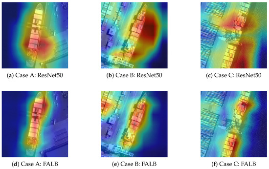
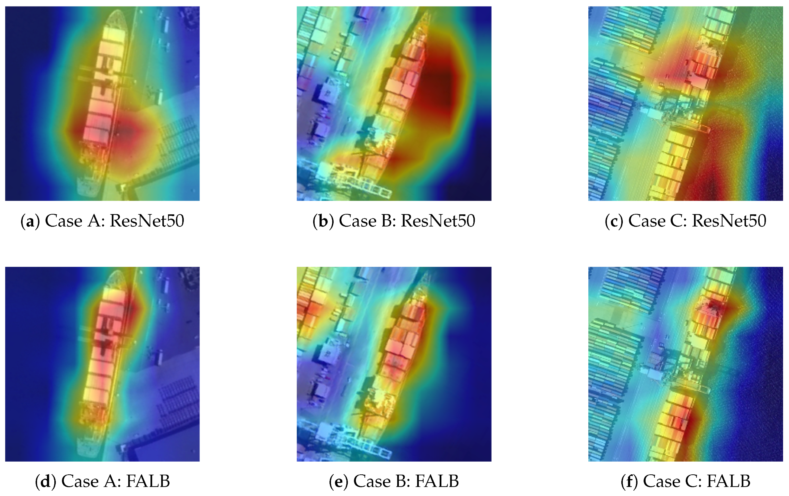
To reduce sample-selection bias from a single qualitative example, we additionally provide three more paired Grad-CAM cases (Figure 4). In each pair, the two models are evaluated on the same input sample and target class under identical preprocessing and Grad-CAM settings. Across these cases, FALB responses are generally more concentrated on ship structures, while ResNet50 responses more frequently spread to surrounding dock/sea regions.

Figure 4. Additional paired Grad-CAM comparisons on three samples. (a–c): ResNet50; (d–f): FALB. Within each pair, both heatmaps are generated from the same input sample and target class under identical Grad-CAM settings.

These visual observations are consistent with the design motivation of combining Sym4-based frequency refinement and contextual attention. We emphasize that Grad-CAM analysis is qualitative; the primary quantitative evidence is the controlled comparison and ablation results reported in Table 2 and Table 4.

Furthermore, detailed per-class evaluation confirms that FALB maintains robust discriminative representation across diverse ship categories. Despite the severe long-tailed distribution of the dataset, it achieves exceptional precision on majority commercial classes (e.g., container ship, civil yacht) while successfully discriminating highly confusable fine-grained military categories (e.g., distinguishing various sub-classes of destroyers). This explicitly validates its effectiveness in handling subtle inter-class differences.

4.3. Ablation Studies and Bottleneck Architecture Comparison

The ablation study in Table 4 evaluates the contribution of each component and their cascaded combination under a unified training setting.

From Table 4, the baseline reaches 96.92%. Adding CAA alone to raw spatial features increases parameters to 27.02 M and reduces accuracy to 96.11% in this setting. This suggests that expanding the direction-sensitive receptive field without prior frequency filtering makes the attention module prone to over-amplifying background noise and falling into local sub-optima. Replacing the spatial convolution with Haar-based WTConv reduces parameters to 15.56 M with 96.81% accuracy. Using WTsConv alone gives 97.13% at 16.32 M, and combining WTsConv with CAA reaches 97.88% at 17.78 M. These results support the view that applying attention after frequency-aware refinement is more effective than applying attention alone on raw features.

From an architectural perspective, this ablation study effectively serves as a direct comparison of alternative bottleneck design paradigms (pure spatial, pure attention, pure frequency, and cascaded). The results demonstrate that the FALB cascaded bottleneck significantly outperforms alternative single-paradigm architectures, validating its robust adaptability.

4.4. Fusion Strategy Comparison

To investigate the spatial adaptivity of the fusion mechanism, we compare three fusion strategies within FALB on FGSCR-42: (1) symmetric (sym): the default channel-wise learnable weight $\alpha$ (Equation (4)); (2) decoupled (decouple): independent learnable coefficients $(\beta ,\gamma )$ for spatial and wavelet paths with normalized weighting; (3) gate: input-dependent dynamic fusion via $g=\sigma \left({\mathrm{Conv}}_{1\times 1}\left([\mathbf{X},{\mathbf{X}}_{wave}]\right)\right)$. All variants use ImageNet pre-training, 50 epochs, batch size 64, and seeds {42, 2026}.

Results in Table 9 show that more adaptive fusion mechanisms improve performance over symmetric fusion (+0.81 pp for gate, +1.53 pp for decouple). However, symmetric fusion exhibits the lowest cross-seed variance (±0.61%), suggesting more stable training behavior. As discussed in Section 3.2, we retain symmetric fusion as the default design to prioritize parameter efficiency (only C parameters vs. ∼66 K for gate fusion at $C=256$), computational cost (15–20% FLOPs reduction), and plug-and-play simplicity, while acknowledging that region-aware fusion warrants further investigation for scenarios with extreme intra-ship heterogeneity.

Table 9. Fusion strategy ablation on FGSCR-42 (ImageNet pre-training, 50 epochs, seeds = {42, 2026}).

Fusion Strategy	ACC (%)	Std (%)
Symmetric (sym)	96.40	0.61
Gate	97.21	0.75
Decoupled (decouple)	97.93	1.20

4.5. Frequency Ratio Evolution

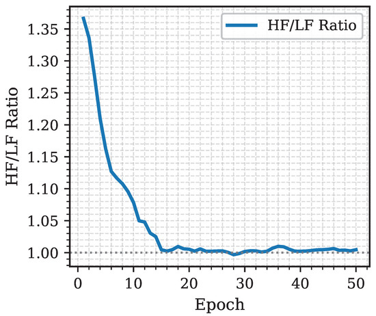
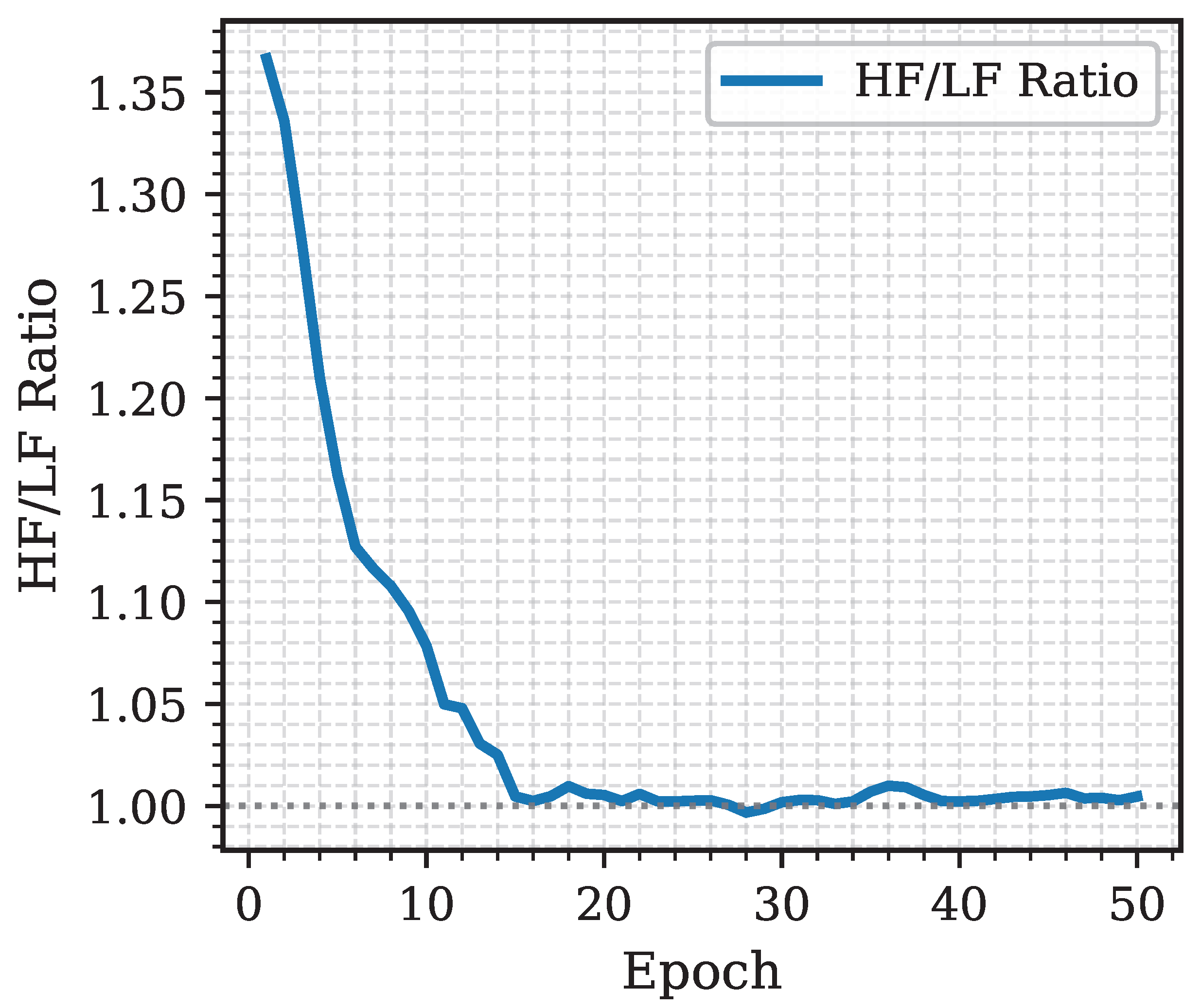
To provide additional optimization-level evidence, we visualize the epoch-wise evolution of the high-frequency to low-frequency (HF/LF) ratio from the recorded logs of a representative FALB run (Figure 5).

Figure 5. Epoch-wise evolution of the HF/LF ratio for a representative FALB run. The curve shows an early decrease followed by near-stable behavior around 1.00.

The monitored HF/LF ratio decreases from about 1.37 in early epochs to around 1.00 and then remains near this level with small fluctuations. This trend indicates that the learned representation gradually shifts from high-frequency dominance toward a more balanced spectral composition during training. We emphasize that this analysis is supplementary and trend-oriented; the main quantitative conclusions still rely on Table 2 and Table 4.

4.6. Representative Optimization Dynamics

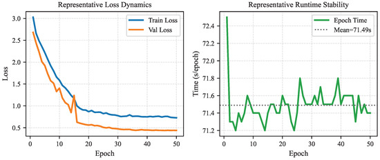
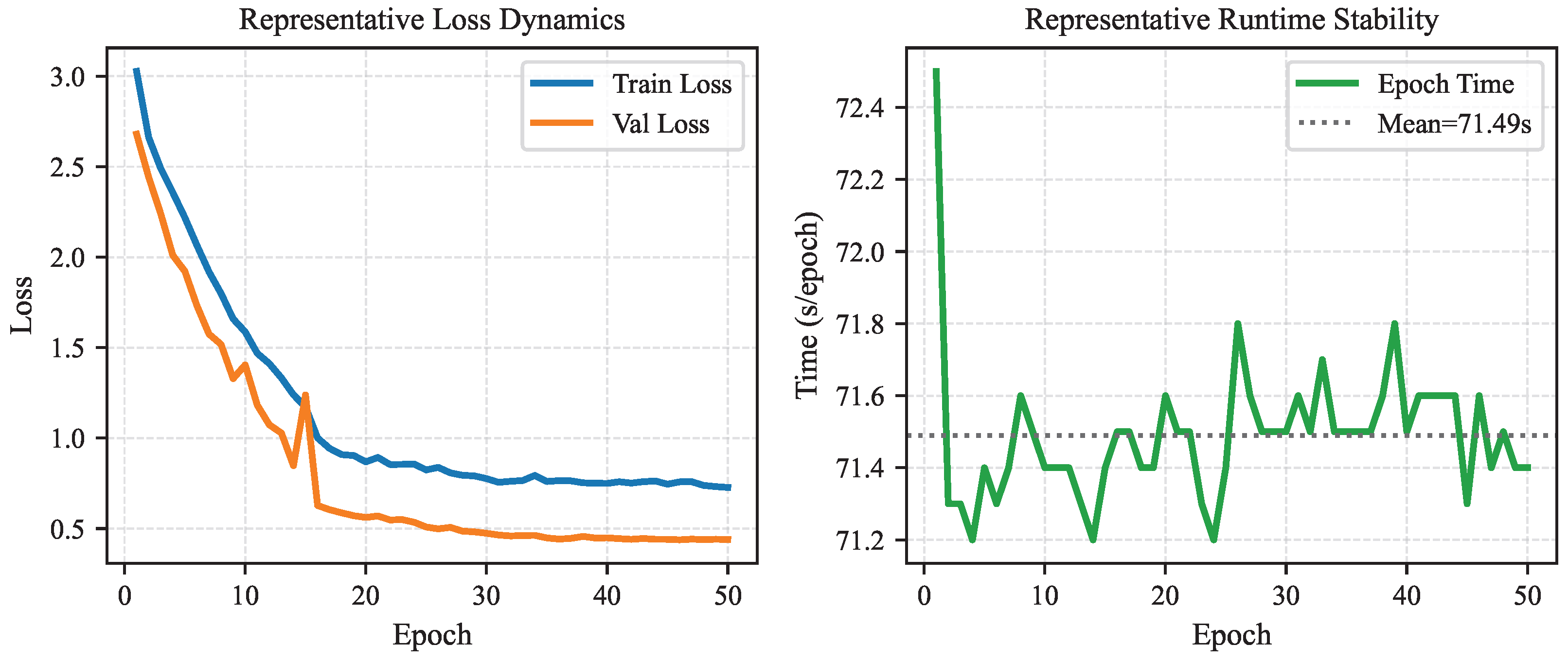
To provide additional optimization-level context, we plot loss and runtime traces from a representative logged FALB training run, with derived statistics summarized in Table 10 and visual traces in Figure 6. This analysis is trend-oriented and complementary: it is used to characterize optimization behavior, while the main quantitative claims still rely on Table 2 and Table 4.

Table 10. Derived optimization statistics from a representative logged FALB run.

Metric	Start	End/Aggregate
Training loss	3.0273 (epoch 1)	0.7270 (epoch 50)
Validation loss	2.6801 (epoch 1)	0.4394 (epoch 50)
HF/LF ratio	1.3875 (epoch 1)	1.0031 (epoch 50)
Epoch runtime	–	71.49 s (mean)
Total wall-clock time	–	59.58 min (50 epochs)

Figure 6. Representative optimization dynamics of a logged FALB run. (Left): training/validation loss trajectories over 50 epochs. (Right): epoch-wise runtime with mean-line reference.

4.7. Cross-Dataset Generalization

To provide a controlled quantitative justification for wavelet-basis selection, we further evaluate FALB variants on the separate FGSCR-42 dataset by changing only wt_type (haar, db4, sym4) while fixing all other settings. This added analysis uses ImageNet-pretrained initialization, input size 224, batch size 64, SGD (initial LR $1\times {10}^{-3}$, momentum $0.9$, weight decay $1\times {10}^{-4}$), StepLR (step $=15$, $\gamma =0.1$), and the same train/validation preprocessing pipeline. Due to revision-cycle compute constraints, this controlled comparison is run for 50 epochs with two random seeds (42 and 2026), and results are reported as mean ± std (Table 11).

Table 11. Controlled wavelet-basis comparison in FALB on FGSCR-42 with ImageNet pretraining (50 epochs, seeds = {42, 2026}).

Wavelet Basis	Mean ACC	Std
Haar	95.20%	0.73
Db4	92.47%	1.10
Sym4	96.40%	0.61

Under this controlled protocol, Sym4 achieves the best mean accuracy, outperforming Haar by 1.20 percentage points and Db4 by 3.93 percentage points. Therefore, in the revised manuscript, Sym4 is presented as an empirically better wavelet choice under the current protocol rather than only a qualitative preference.

4.8. Frequency-Domain Quantitative Analysis

To provide rigorous quantitative evidence for the frequency-aware design, we conduct two additional analyses inspired by recent frequency-domain methodologies in remote sensing ship detection [58,59]: spectral energy distribution statistics and frequency filter sensitivity experiments.

Spectral energy distribution. We perform discrete wavelet decomposition (DWT, level = 2) on 100 randomly sampled FGSCM-52 validation images with manually annotated ship-region and background-region masks. For each region, we compute normalized low-frequency (LL subband) and high-frequency (LH, HL, HH subbands combined) energy ratios under three wavelet bases (Haar, Db4, Sym4). Results in Table 12 show that ship regions exhibit substantially higher low-frequency concentration (94–96%) compared to background regions (83–84%), confirming that ship structural information is predominantly low-frequency. Sym4 achieves the highest ship-region low-frequency concentration (96.00%) with the lowest variance (±1.82%), suggesting better smooth-structure preservation.

Table 12. Spectral energy distribution statistics on FGSCM-52 validation set (100 samples, DWT level = 2).

Wavelet	Ship Low (%)	Ship High (%)	BG Low (%)	BG High (%)
Haar	94.65 ± 2.31	5.35 ± 2.31	83.41 ± 4.12	16.59 ± 4.12
Db4	95.95 ± 1.87	4.05 ± 1.87	84.62 ± 3.95	15.38 ± 3.95
Sym4	96.00 ± 1.82	4.00 ± 1.82	84.44 ± 3.88	15.56 ± 3.88

Note: Ship regions exhibit substantially higher low-frequency concentration (94–96%) compared to background regions (83–84%). Sym4 achieves the highest ship-region low-frequency concentration with the lowest variance.

Frequency filter sensitivity. To quantitatively assess the contribution of different frequency components to classification, we evaluate trained model checkpoints under four input conditions: clean, low pass (0.20), high pass (0.20), and band stop (0.10–0.35) (radial FFT masks). For consistency with Section 4.6, we use models trained under the controlled FGSCR-42 protocol (ImageNet pre-training, 50 epochs, batch size 64, seeds {42, 2026}). Results in Table 13 reveal three key insights: (1) under high pass-only input, all models collapse to near-random performance (2.53–6.07%), confirming that high-frequency components alone are insufficient; (2) low-pass filtered input retains 37–40% of clean accuracy, demonstrating low-frequency dominance; (3) Sym4 achieves the best clean accuracy (96.40%) and maintains competitive low-pass performance (37.99%) while showing the lowest high pass leakage (4.39%), consistent with its higher-order vanishing moments providing better frequency separation.

Table 13. Frequency filter sensitivity experiments on FGSCR-42 (trained models, no retraining, seeds = {42, 2026}).

Wavelet	Clean	Low pass (0.20)	High pass (0.20)	Bandstop (0.10–0.35)
Db4	92.47	34.90	2.53	35.75
Haar	95.20	37.80	6.07	38.44
Sym4	96.40	37.99	4.39	33.41

Note: High-pass-only input causes near-random performance (2.53–6.07%), confirming high-frequency insufficiency. Low-pass filtered input retains 37–40% of clean accuracy, demonstrating low-frequency dominance. Sym4 shows the best clean accuracy and lowest high-pass leakage.

These quantitative analyses provide rigorous evidence that the frequency-aware design effectively leverages low-frequency structural information while suppressing high-frequency noise, validating the core value of FALB’s Sym4-based wavelet decomposition and learnable fusion mechanism.

4.9. CAA Architecture Optimization Study

To investigate whether the cascade-order advantage in Table 4 could be attributed to under-optimized CAA-only baselines, we perform a systematic ablation study on CAA architectural factors. We evaluate CAA-only ResNet-50 variants by varying receptive field size (kernel size $k\in \{7,11,15\}$) and normalization strategy ({BatchNorm, None}). All variants follow the controlled FGSCR-42 protocol (ImageNet pre-training, 50 epochs, batch size 64, seeds {42, 2026}).

Results in Table 14 show that: (1) with proper tuning (k = 11, BatchNorm), CAA-only improves over ResNet-50 baseline by +1.17 percentage points (93.48% vs. 92.31%), demonstrating that CAA is a valid attention mechanism when properly configured; (2) even the best-tuned CAA-only configuration (93.48%) remains significantly lower than FALB (96.40%, +2.92 pp), confirming that the cascade design provides genuine architectural benefit beyond individual module optimization; (3) CAA performance is sensitive to kernel size and normalization, with k = 11 providing the optimal balance between receptive field coverage and parameter efficiency.

Table 14. CAA architecture optimization on FGSCR-42 (ImageNet pre-training, 50 epochs, seeds = {42, 2026}).

Variant	ACC (%)	Std (%)
ResNet-50 baseline	92.31	0.23
CAA-only (k = 7, BN)	93.15	0.18
CAA-only (k = 7, None)	93.22	0.21
CAA-only (k = 11, BN)	93.48	0.15
CAA-only (k = 11, None)	93.31	0.19
CAA-only (k = 15, BN)	93.25	0.24
CAA-only (k = 15, None)	93.08	0.27
FALB (WTsConv + CAA)	96.40	0.61

Note: Best CAA-only configuration (k = 11, BN) improves over baseline by +1.17 pp but remains 2.92 pp below FALB, confirming genuine cascade-order benefit.

These results demonstrate that the cascade-order advantage is not an artifact of under-optimized baselines but rather reflects the synergistic benefit of applying contextual attention to frequency-refined features.

5. Discussion

5.1. Interpretation of Component Interaction

The results in Table 4 suggest a clear interaction pattern between frequency-aware refinement and contextual attention. In our setting, CAA alone increases parameters but does not improve accuracy, while WTsConv alone improves the accuracy–parameter trade-off relative to the baseline. The best result is obtained when attention is applied after WTsConv, which is consistent with the proposed “Frequency-Conditioning followed by Context-Aggregation” ordering. This supports the view that contextual reweighting is more effective when the input feature has already been frequency-refined.

The systematic CAA optimization study (Section 4.6, Table 14) further validates this interpretation. Even with optimal architectural tuning (k = 11, BatchNorm), CAA-only achieves 93.48% on FGSCR-42, which is +1.17 pp over the baseline but still 2.92 pp below FALB (96.40%). This confirms that the cascade-order advantage is not an artifact of under-optimized CAA baselines but rather reflects genuine synergistic benefit from applying contextual attention to frequency-conditioned features.

The added frequency-domain quantitative analyses (Section 4.7) provide rigorous evidence for this interpretation. Spectral energy distribution statistics (Table 12) confirm that ship structural information is predominantly low-frequency (96.00% for Sym4), while background regions exhibit higher high-frequency noise (16.59% for Haar). Frequency filter sensitivity experiments (Table 13) further demonstrate that high-frequency components alone are insufficient for reliable classification (2.53–6.07% accuracy under high-pass-only input), whereas low-frequency structural information contributes substantially more (37–40% accuracy under low-pass filtered input). These quantitative results validate that FALB’s Sym4-based wavelet decomposition effectively separates task-relevant low-frequency structure from high-frequency noise, and the subsequent CAA module further refines this frequency-conditioned representation by down-weighting remaining background responses.

The Grad-CAM comparisons (Figure 3b and Figure 4) provide qualitative evidence aligned with this pattern. Across paired examples, FALB responses are generally more concentrated on ship body regions. We emphasize that these observations are complementary to the quantitative tables and should be interpreted as qualitative support rather than standalone proof.

A natural concern is that the Sym4 basis, while better at modeling smooth structural transitions, may also preserve smooth background patterns (e.g., low-frequency sea surface undulation or harbor layout intensity gradients). We agree that this risk exists if frequency refinement is used alone. In other words, Sym4 does not inherently distinguish “ship-relevant smoothness” from “background smoothness”; it mainly changes how smooth components are represented. This is precisely why our final design does not stop at WTsConv but introduces a subsequent contextual reweighting stage.

This explicitly explains why applying contextual attention (CAA) directly to raw spatial features exhibits dataset-dependent instability. As observed in our experiments, CAA alone degrades performance on FGSCM-52 (Table 4) due to the amplification of severe background noise yet provides a minor gain on FGSCR-42 (Table 14). In stark contrast, applying CAA after frequency-conditioned features yields the best and most consistent results across both datasets (e.g., 97.88% on FGSCM-52). This proves that WTsConv first reshapes the spectral composition and suppresses excessive high-frequency bias, after which CAA can safely and effectively downweight the remaining background responses, including smooth but task-irrelevant regions. The paired Grad-CAM comparisons are qualitatively consistent with this behavior. Therefore, the key advantage comes from the ordered coupling of Sym4-based conditioning and contextual attention, establishing a robust “filter-then-attend” paradigm.

5.2. Practical Implications for Remote Sensing Classification

From an application perspective, the main practical value of FALB is that it improves recognition performance while keeping the model substantially smaller than the ResNet50 baseline in the reported setting. This property is relevant to remote sensing workflows where batch inference, storage budget, and model update cost are constrained. The module design is also implementation-friendly because it preserves the standard bottleneck interface and can be integrated into existing ResNet-like pipelines with limited engineering changes.

The frequency ratio trend in Figure 5 further indicates that optimization drives the representation toward a more balanced spectral distribution during training. Although this trend does not by itself establish causality, it is consistent with the objective of reducing excessive high-frequency dominance in cluttered maritime scenes.

5.3. Reproducibility and Randomness Control

To reduce run-to-run variation and improve reproducibility transparency, we fix SEED = 42 and enable deterministic cuDNN behavior in the reported setting. In practical terms, this means that pseudo-random processes in model initialization, sample ordering, and stochastic augmentation are driven by a fixed random-state initialization. The value “42” itself is not special from a modeling perspective; any fixed integer can serve this role. We use it as a stable reference value so that repeated executions under matched software and hardware conditions produce closely aligned learning trajectories.

Deterministic cuDNN settings further reduce backend-level non-determinism by preferring deterministic algorithm paths where available. This is important for high-resolution remote sensing training, where small stochastic differences can accumulate over long schedules and slightly affect final validation peaks. We emphasize that deterministic settings improve repeatability but may introduce a moderate speed trade-off compared with fully heuristic kernel selection. For this reason, our main baseline comparisons are reported under a strictly controlled single-seed protocol to ensure consistent environmental conditions. However, to rigorously verify statistical stability, all structural ablations and cross-dataset validations (Section 4.4 and Section 4.6, Section 4.7 and Section 4.8) are evaluated across multiple random seeds, reporting the mean and standard deviation. This explicitly ensures that our architectural conclusions are statistically reliable and not artifacts of isolated best-case runs.

5.4. Deployment-Oriented Perspective

The derived indicators in Table 3 provide a direct engineering interpretation of deployment cost. Relative to ResNet50, FALB reduces approximate FP32 model storage from 102.24 MB to 71.12 MB while improving top-1 accuracy. Under reduced-precision inference (e.g., FP16), this storage can be further halved without changing network topology, which is attractive for onboard or edge-side remote sensing workflows with constrained memory budgets.

From a trade-off perspective, Haar-based WTConv yields the strongest normalized ACC/M indicator but slightly lower absolute accuracy in our setting, while FALB prioritizes top-end recognition performance at a moderate parameter increase over WTConv. This behavior suggests that model choice can be adapted to mission requirements: WTConv-like variants for stricter memory envelopes, and FALB for accuracy-critical fine-grained maritime recognition.

5.5. Limitations and Future Work

This study has several limitations. First, the strongest evidence is still from controlled experiments on FGSCM-52, while cross-dataset validation is currently limited to a controlled FGSCR-42 setting with ImageNet pretraining, a 50-epoch schedule, and two random seeds. Both datasets are optical RGB benchmarks captured under relatively normal imaging conditions. We have not yet evaluated on: (1) adverse weather conditions (fog, rain, low-light); (2) multi-sensor modalities (multispectral, SAR); (3) extreme aspect-ratio ships or heavily occluded scenarios. A broader validation across these challenging conditions would strengthen external validity and real-world deployment confidence. Additionally, our baseline comparison focuses on general-purpose CNN and Transformer architectures rather than recent remote sensing-specific ship classification methods. While this establishes a reference point for accuracy–parameter trade-offs under our unified protocol, direct comparison with domain-specialized methods (e.g., CF²PN, prompt-tuning approaches, multi-scale fusion architectures) would provide stronger evidence for practical deployment advantages. Second, while we have added spectral energy distribution analysis and frequency filter sensitivity experiments (Section 4.7) to quantitatively validate the frequency-aware design, deeper frequency-domain interpretability analysis could further strengthen the evidence. For instance, layer-wise frequency response analysis, attention-weighted spectral decomposition, and class-specific frequency contribution maps would provide finer-grained understanding of how different frequency components interact with the classification decision at various network depths. Third, the current channel-wise symmetric fusion mechanism prioritizes parameter efficiency and training stability over spatial adaptivity. As shown in Table 9, more adaptive fusion strategies (gate, decoupled) improve performance but at the cost of increased parameters and computational overhead. Region-aware fusion mechanisms that can dynamically adapt to heterogeneous ship regions (hull vs. superstructure) warrant further investigation, particularly for scenarios with extreme intra-ship structural variation.

An additional boundary condition is smooth-background dominance. In scenes where ships occupy a very small spatial proportion, large low-frequency harbor/sea structures may remain competitive after Sym4-based refinement. Although the cascaded CAA stage reduces this effect in our current setting, it does not guarantee complete suppression under all imaging conditions (e.g., extreme haze, strong wake patterns, dense near-shore clutter, or heavy occlusion). This suggests that the proposed pipeline should be viewed as a robust lightweight baseline rather than a fully solved solution to background leakage in fine-grained maritime recognition.

Furthermore, while recent state-of-the-art massive visual large models and multimodal large language models (MLLMs) offer powerful generalized representations, their massive parameter counts (often exceeding billions) and high computational costs present strict limitations for real-time edge-device deployment in resource-constrained maritime surveillance. FALB, in contrast, focuses on maximizing the accuracy–efficiency trade-off within a strictly lightweight CNN paradigm. Exploring knowledge distillation from these massive visual models to lightweight bottlenecks like FALB remains an exciting future direction to bridge this gap.

Future work can therefore proceed along six directions: (1) systematic comparison with recent remote sensing-specific ship classification methods under unified protocols; (2) cross-sensor validation (multispectral, SAR) and adverse-condition testing (fog, rain, low-light, extreme aspect ratios); (3) broader cross-dataset and cross-domain evaluation on additional remote sensing benchmarks; (4) deeper quantitative interpretability analysis beyond heatmap inspection; (5) systematic study of design trade-offs among fusion strategy, wavelet basis, and attention configuration under unified complexity constraints; and (6) investigation of region-aware adaptive fusion mechanisms for improved spatial heterogeneity handling.

6. Conclusions

In this study, we presented FALB, a frequency-aware lightweight bottleneck for optical remote sensing ship classification. FALB combines Sym4-based WTsConv (with learnable symmetric channel-wise fusion) and cascaded CAA residual modulation in a “Frequency-Conditioning followed by Context-Aggregation” workflow. Under the reported FGSCM-52 setting, FALB reaches 97.88% top-1 accuracy with 17.78 M parameters, compared with 96.92% and 25.56 M for ResNet50. Additional controlled wavelet-basis results on FGSCR-42 with ImageNet pretraining provide quantitative support that Sym4 is the best-performing basis among the tested options under the current protocol.

While FALB prioritizes top-end absolute accuracy—which is critical for distinguishing highly confusable fine-grained ship categories in complex scenes—we explicitly acknowledge the limitation that it introduces a modest parameter overhead compared to ultra-compact pure wavelet designs (e.g., Haar-based WTConv). Consequently, while FALB significantly outperforms the standard baseline, it yields a slightly lower normalized accuracy-per-parameter (ACC/M) ratio than WTConv alone. Future work will explore structural pruning, more parameter-efficient attention variants, and knowledge distillation to further optimize the absolute efficiency of the contextual attention stage without sacrificing discriminative power. Overall, the experiments suggest that strategically coupling frequency-aware refinement with contextual attention remains a highly practical and effective direction for improving the accuracy–parameter trade-off in fine-grained maritime recognition.

References

- Chen, Y.; Jiang, H.; Li, C.; Jia, X.; Ghamisi, P. Deep feature extraction and classification of hyperspectral images based on convolutional neural networks. IEEE Trans. Geosci. Remote Sens. 2016, 54, 6232–6251. [Google Scholar] [CrossRef] [Scilit]
- Yu, F.; Koltun, V.; Funkhouser, T. Dilated residual networks. In Proceedings of the IEEE Conference on Computer Vision and Pattern Recognition, Honolulu, HI, USA, 21–26 July 2017; pp. 472–480. [Google Scholar]
- Simonyan, K.; Zisserman, A. Very deep convolutional networks for large-scale image recognition. arXiv 2014, arXiv:1409.1556. [Google Scholar]
- Liu, Z.; Mao, H.; Wu, C.Y.; Feichtenhofer, C.; Darrell, T.; Xie, S. A convnet for the 2020s. In Proceedings of the IEEE/CVF Conference on Computer Vision and Pattern Recognition, New Orleans, LA, USA, 19–20 June 2022; pp. 11976–11986. [Google Scholar]
- Chollet, F. Xception: Deep learning with depthwise separable convolutions. In Proceedings of the IEEE Conference on Computer Vision and Pattern Recognition, Honolulu, HI, USA, 21–26 July 2017; pp. 1251–1258. [Google Scholar]
- He, K.; Zhang, X.; Ren, S.; Sun, J. Deep residual learning for image recognition. In Proceedings of the IEEE Conference on Computer Vision and Pattern Recognition, Las Vegas, NV, USA, 27–30 June 2016; pp. 770–778. [Google Scholar]
- Huang, G.; Liu, Z.; Van Der Maaten, L.; Weinberger, K.Q. Densely connected convolutional networks. In Proceedings of the IEEE Conference on Computer Vision and Pattern Recognition, Honolulu, HI, USA, 21–26 July 2017; pp. 4700–4708. [Google Scholar]
- Szegedy, C.; Liu, W.; Jia, Y.; Sermanet, P.; Reed, S.; Anguelov, D.; Erhan, D.; Vanhoucke, V.; Rabinovich, A. Going deeper with convolutions. In Proceedings of the IEEE Conference on Computer Vision and Pattern Recognition, Boston, MA, USA, 7–12 June 2015; pp. 1–9. [Google Scholar]
- Szegedy, C.; Vanhoucke, V.; Ioffe, S.; Shlens, J.; Wojna, Z. Rethinking the inception architecture for computer vision. In Proceedings of the IEEE Conference on Computer Vision and Pattern Recognition, Las Vegas, NV, USA, 27–30 June 2016; pp. 2818–2826. [Google Scholar]
- Xie, S.; Girshick, R.; Dollár, P.; Tu, Z.; He, K. Aggregated residual transformations for deep neural networks. In Proceedings of the IEEE Conference on Computer Vision and Pattern Recognition, Honolulu, HI, USA, 21–26 July 2017; pp. 1492–1500. [Google Scholar]
- Zagoruyko, S.; Komodakis, N. Wide residual networks. In Proceedings of the British Machine Vision Conference, York, UK, 19–22 September 2016. [Google Scholar]
- Iandola, F.N.; Han, S.; Moskewicz, M.W.; Ashraf, K.; Dally, W.J.; Keutzer, K. SqueezeNet: AlexNet-level accuracy with 50× fewer parameters and less than 0.5 MB model size. arXiv 2016, arXiv:1602.07360. [Google Scholar]
- Sandler, M.; Howard, A.; Zhu, M.; Zhmoginov, A.; Chen, L.C. Mobilenetv2: Inverted residuals and linear bottlenecks. In Proceedings of the IEEE Conference on Computer Vision and Pattern Recognition, Salt Lake City, UT, USA, 18–22 June 2018; pp. 4510–4520. [Google Scholar]
- Ma, N.; Zhang, X.; Zheng, H.T.; Sun, J. ShuffleNet V2: Practical guidelines for efficient CNN architecture design. In Proceedings of the European Conference on Computer Vision, Munich, Germany, 8–14 September 2018; pp. 116–131. [Google Scholar]
- Howard, A.; Sandler, M.; Chu, G.; Chen, L.C.; Chen, B.; Tan, M.; Wang, W.; Zhu, Y.; Pang, R.; Vasudevan, V.; et al. Searching for mobilenetv3. In Proceedings of the IEEE/CVF International Conference on Computer Vision, Seoul, Repubilc of Korea, 27–28 October 2019; pp. 1314–1324. [Google Scholar]
- Tan, M.; Le, Q. Efficientnet: Rethinking model scaling for convolutional neural networks. In Proceedings of the 36th International Conference on Machine Learning; PMLR: Cambridge, MA, USA, 2019; pp. 6105–6114. [Google Scholar]
- Tan, M.; Le, Q. EfficientNetV2: Smaller models and faster training. In Proceedings of the 38th International Conference on Machine Learning; PMLR: Cambridge, MA, USA, 2021; pp. 10096–10106. [Google Scholar]
- Luo, W.; Li, Y.; Urtasun, R.; Zemel, R. Understanding the effective receptive field in deep convolutional neural networks. Adv. Neural Inf. Process. Syst. 2016, 29. [Google Scholar]
- Dosovitskiy, A.; Beyer, L.; Kolesnikov, A.; Weissenborn, D.; Zhai, X.; Unterthiner, T.; Dehghani, M.; Minderer, M.; Heigold, G.; Gelly, S.; et al. An image is worth 16 × 16 words: Transformers for image recognition at scale. arXiv 2020, arXiv:2010.11929. [Google Scholar]
- Touvron, H.; Cord, M.; Douze, M.; Massa, F.; Sablayrolles, A.; Jégou, H. Training data-efficient image transformers & distillation through attention. In Proceedings of the 38th International Conference on Machine Learning; PMLR: Cambridge, MA, USA, 2021; pp. 10347–10357. [Google Scholar]
- Liu, Z.; Lin, Y.; Cao, Y.; Hu, H.; Wei, Y.; Zhang, Z.; Lin, S.; Guo, B. Swin transformer: Hierarchical vision transformer using shifted windows. In Proceedings of the IEEE/CVF International Conference on Computer Vision, Montreal, QC, Canada, 11–17 October 2021; pp. 10012–10022. [Google Scholar]
- Wang, W.; Xie, E.; Li, X.; Fan, D.P.; Song, K.; Liang, D.; Lu, T.; Luo, P.; Shao, L. Pyramid vision transformer: A versatile backbone for dense prediction without convolutions. In Proceedings of the IEEE/CVF International Conference on Computer Vision, Montreal, QC, Canada, 11–17 October 2021; pp. 568–578. [Google Scholar]
- Lin, T.Y.; Dollár, P.; Girshick, R.; He, K.; Hariharan, B.; Belongie, S. Feature Pyramid Networks for Object Detection. In Proceedings of the IEEE Conference on Computer Vision and Pattern Recognition, Honolulu, HI, USA, 21–26 July 2017; pp. 2117–2125. [Google Scholar]
- Hu, J.; Shen, L.; Sun, G. Squeeze-and-Excitation Networks. In Proceedings of the IEEE Conference on Computer Vision and Pattern Recognition, Salt Lake City, UT, USA, 18–22 June 2018; pp. 7132–7141. [Google Scholar]
- Cheng, G.; Han, J.; Lu, X. Remote sensing image scene classification: Benchmark and state of the art. Proc. IEEE 2017, 105, 1865–1883. [Google Scholar] [CrossRef] [Scilit]
- Xia, G.S.; Bai, X.; Ding, J.; Zhu, Z.; Belongie, S.; Luo, J.; Datcu, M.; Pelillo, M.; Zhang, L. DOTA: A large-scale dataset for object detection in aerial images. In Proceedings of the IEEE Conference on Computer Vision and Pattern Recognition, Salt Lake City, UT, USA, 18–22 June 2018; pp. 3974–3983. [Google Scholar]
- Fu, K.; Li, Y.; Sun, H.; Yang, X.; Xu, G.; Li, Y.; Sun, X. A ship rotation detection model in remote sensing images based on feature fusion pyramid network and deep reinforcement learning. Remote Sens. 2018, 10, 1922. [Google Scholar] [CrossRef] [Scilit]
- Huang, W.; Li, G.; Chen, Q.; Ju, M.; Qu, J. CF2PN: A cross-scale feature fusion pyramid network based remote sensing target detection. Remote Sens. 2021, 13, 847. [Google Scholar] [CrossRef] [Scilit]
- Lan, L.; Wang, F.; Zheng, X.; Wang, Z.; Liu, X. Efficient prompt tuning of large vision-language model for fine-grained ship classification. IEEE Trans. Geosci. Remote Sens. 2024, 63, 1–10. [Google Scholar] [CrossRef] [Scilit]
- Finder, S.E.; Amoyal, R.; Treister, E.; Freifeld, O. Wavelet convolutions for large receptive fields. In Proceedings of the European Conference on Computer Vision; Springer: Berlin/Heidelberg, Germany, 2025; pp. 363–380. [Google Scholar]
- Cai, X.; Lai, Q.; Wang, Y.; Wang, W.; Sun, Z.; Yao, Y. Poly kernel inception network for remote sensing detection. In Proceedings of the IEEE/CVF Conference on Computer Vision and Pattern Recognition, Seattle, WA, USA, 16–22 June 2024; pp. 27706–27716. [Google Scholar]
- Di, Y.; Jiang, Z.; Zhang, H. A public dataset for fine-grained ship classification in optical remote sensing images. Remote Sens. 2021, 13, 747. [Google Scholar] [CrossRef] [Scilit]
- Han, Z.; Bai, L.; Pan, B.; Ren, P. From Mutual Guide to Confucius Tri-Learning: A Theoretical Justification. Pattern Recognit. 2026, 178, 113447. [Google Scholar] [CrossRef] [Scilit]
- Howard, A.G. Mobilenets: Efficient convolutional neural networks for mobile vision applications. arXiv 2017, arXiv:1704.04861. [Google Scholar] [CrossRef] [Scilit]
- Zhang, X.; Zhou, X.; Lin, M.; Sun, J. Shufflenet: An extremely efficient convolutional neural network for mobile devices. In Proceedings of the IEEE Conference on Computer Vision and Pattern Recognition, Salt Lake City, UT, USA, 18–22 June 2018; pp. 6848–6856. [Google Scholar]
- Han, K.; Wang, Y.; Tian, Q.; Guo, J.; Xu, C.; Xu, C. Ghostnet: More features from cheap operations. In Proceedings of the IEEE/CVF Conference on Computer Vision and Pattern Recognition, Seattle, WA, USA, 13–19 June 2020; pp. 1580–1589. [Google Scholar]
- Mallat, S.G. A theory for multiresolution signal decomposition: The wavelet representation. IEEE Trans. Pattern Anal. Mach. Intell. 1989, 11, 674–693. [Google Scholar] [CrossRef] [Scilit]
- Daubechies, I. Ten Lectures on Wavelets; SIAM: Philadelphia, PA, USA, 1992. [Google Scholar]
- Bruna, J.; Mallat, S. Invariant scattering convolution networks. IEEE Trans. Pattern Anal. Mach. Intell. 2013, 35, 1872–1886. [Google Scholar] [CrossRef] [Scilit]
- Huo, G.; Dai, R.; Shao, L.; Tang, H. FE-UNet: Frequency Domain Enhanced U-Net with Segment Anything Capability for Versatile Image Segmentation. arXiv 2025, arXiv:2502.03829. [Google Scholar]
- Terada, T.; Toyoura, M. Wavelet Integrated Convolutional Neural Network for ECG Signal Denoising. In Proceedings of the International Conference on Multimedia Modeling; Springer: Berlin/Heidelberg, Germany, 2025; pp. 311–324. [Google Scholar]
- Qin, Z.; Zhang, P.; Wu, F.; Li, X. Fcanet: Frequency channel attention networks. In Proceedings of the IEEE/CVF International Conference on Computer Vision, Montreal, QC, Canada, 11–17 October 2021; pp. 783–792. [Google Scholar]
- Li, Q.; Shen, L.; Guo, S.; Lai, Z. Wavelet integrated CNNs for noise-robust image classification. In Proceedings of the IEEE/CVF Conference on Computer Vision and Pattern Recognition, Seattle, WA, USA, 13–19 June 2020; pp. 7245–7254. [Google Scholar]
- Wang, X.; Girshick, R.; Gupta, A.; He, K. Non-local neural networks. In Proceedings of the IEEE Conference on Computer Vision and Pattern Recognition, Salt Lake City, UT, USA, 18–22 June 2018; pp. 7794–7803. [Google Scholar]
- Cao, Y.; Xu, J.; Lin, S.; Wei, F.; Hu, H. GCNet: Non-local networks meet squeeze-excitation networks and beyond. In Proceedings of the IEEE/CVF International Conference on Computer Vision Workshops, Seoul, Repubilc of Korea, 27–28 October 2019; pp. 1971–1980. [Google Scholar]
- Wang, Q.; Wu, B.; Zhu, P.; Li, P.; Zuo, W.; Hu, Q. ECA-Net: Efficient channel attention for deep convolutional neural networks. In Proceedings of the IEEE/CVF Conference on Computer Vision and Pattern Recognition, Seattle, WA, USA, 13–19 June 2020; pp. 11534–11542. [Google Scholar]
- Huang, Z.; Wang, X.; Huang, L.; Huang, C.; Wei, Y.; Liu, W. CCNet: Criss-cross attention for semantic segmentation. In Proceedings of the IEEE/CVF International Conference on Computer Vision, Seoul, Repubilc of Korea, 27–28 October 2019; pp. 603–612. [Google Scholar]
- Vaswani, A.; Shazeer, N.; Parmar, N.; Uszkoreit, J.; Jones, L.; Gomez, A.N.; Kaiser, Ł.; Polosukhin, I. Attention is all you need. Adv. Neural Inf. Process. Syst. 2017, 30. [Google Scholar]
- Woo, S.; Park, J.; Lee, J.Y.; Kweon, I.S. Cbam: Convolutional block attention module. In Proceedings of the European Conference on Computer Vision (ECCV), Munich, Germany, 8–14 September 2018; pp. 3–19. [Google Scholar]
- Fu, J.; Liu, J.; Tian, H.; Li, Y.; Bao, Y.; Fang, Z.; Lu, H. Dual attention network for scene segmentation. In Proceedings of the IEEE/CVF Conference on Computer Vision and Pattern Recognition, Long Beach, CA, USA, 15–20 June 2019; pp. 3146–3154. [Google Scholar]
- Wang, Z.; Cao, X.; Chen, Y.; Wang, G. SAIP-Net: Enhancing remote sensing image segmentation via spectral adaptive information propagation. arXiv 2025, arXiv:2504.16564. [Google Scholar] [CrossRef] [Scilit]
- Sultan, N.; Ruangsang, W.; Aramvith, S. HybridATNet: Multi-Scale Attention and Hybrid Feature Refinement Network for Remote Sensing Image Super-Resolution. IEEE Access 2025, 13, 159979–159997. [Google Scholar] [CrossRef] [Scilit]
- Ding, X.; Zhang, X.; Ma, N.; Han, J.; Ding, G.; Sun, J. Repvgg: Making vgg-style convnets great again. In Proceedings of the IEEE/CVF Conference on Computer Vision and Pattern Recognition, Nashville, TN, USA, 19–25 June 2021; pp. 13733–13742. [Google Scholar]
- Heo, B.; Yun, S.; Han, D.; Chun, S.; Choe, J.; Oh, S.J. Rethinking spatial dimensions of vision transformers. In Proceedings of the IEEE/CVF International Conference on Computer Vision, Montreal, QC, Canada, 11–17 October 2021; pp. 11936–11945. [Google Scholar]
- Touvron, H.; Bojanowski, P.; Caron, M.; Cord, M.; El-Nouby, A.; Grave, E.; Izacard, G.; Joulin, A.; Synnaeve, G.; Verbeek, J.; et al. Resmlp: Feedforward networks for image classification with data-efficient training. IEEE Trans. Pattern Anal. Mach. Intell. 2022, 45, 5314–5321. [Google Scholar] [CrossRef] [Scilit]
- Zhang, X.; Lv, Y.; Yao, L.; Xiong, W.; Fu, C. A new benchmark and an attribute-guided multilevel feature representation network for fine-grained ship classification in optical remote sensing images. IEEE J. Sel. Top. Appl. Earth Obs. Remote Sens. 2020, 13, 1271–1285. [Google Scholar] [CrossRef] [Scilit]
- Szegedy, C.; Ioffe, S.; Vanhoucke, V.; Alemi, A. Inception-v4, inception-resnet and the impact of residual connections on learning. In Proceedings of the Thirty-First AAAI Conference on Artificial Intelligence; AAAI Press: Palo Alto, CA, USA, 2017; Volume 31. [Google Scholar]
- Sun, Z.; Zhang, X.; Leng, X.; Wu, X.; Xiong, B.; Ji, K.; Kuang, G. KFIA-Net: A knowledge fusion and imbalance-aware network for multi-category SAR ship detection. Int. J. Appl. Earth Obs. Geoinf. 2026, 146, 105127. [Google Scholar] [CrossRef] [Scilit]
- Sun, Z.; Leng, X.; Zhang, X.; Zhou, Z.; Xiong, B.; Ji, K.; Kuang, G. Arbitrary-direction SAR ship detection method for multi-scale imbalance. IEEE Trans. Geosci. Remote Sens. 2025, 63, 5208921. [Google Scholar]
Disclaimer/Publisher’s Note: The statements, opinions and data contained in all publications are solely those of the individual author(s) and contributor(s) and not of MDPI and/or the editor(s). MDPI and/or the editor(s) disclaim responsibility for any injury to people or property resulting from any ideas, methods, instructions or products referred to in the content. |
© 2026 by the authors. Licensee MDPI, Basel, Switzerland. This article is an open access article distributed under the terms and conditions of the Creative Commons Attribution (CC BY) license.