Author Contributions
Methodology, Y.S.; Software, Y.S.; Validation, Y.S.; Data curation, H.Y.; Writing—original draft, Y.S.; Writing—review & editing, Y.S.; Visualization, Y.S.; Supervision, L.H., Q.S., L.C. and X.Z.; Funding acquisition, L.H. All authors have read and agreed to the published version of the manuscript.
Figure 1.
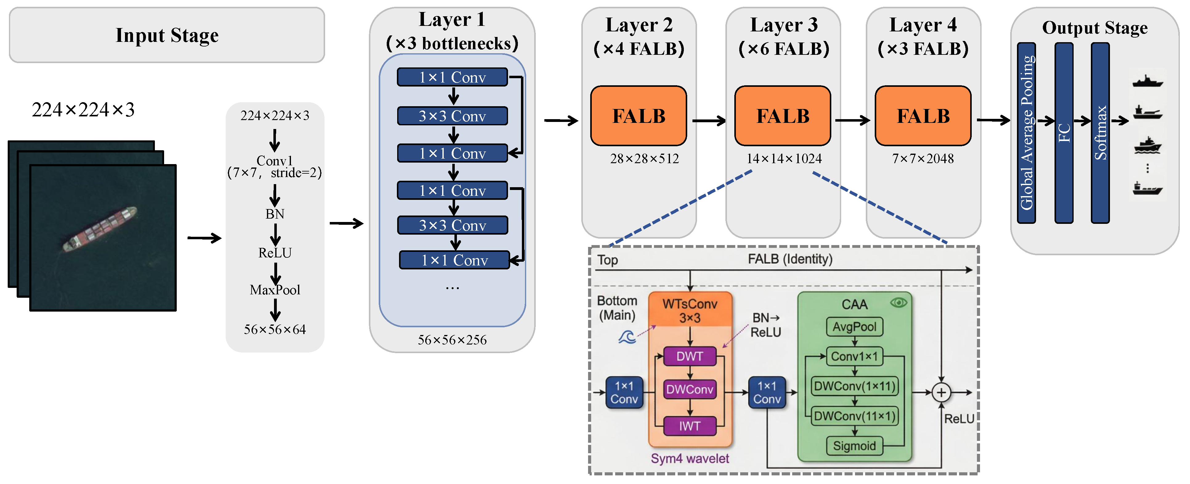
Overview of FALB integration into ResNet50. Bottlenecks in Layer 1 (
) remain unchanged, while bottlenecks in Layers 2–4 (
) are replaced by the proposed FALB bottleneck. The lower panel shows the cascaded path
Conv → WTsConv → BN/ReLU →
Conv → CAA, followed by identity addition (with downsample when needed) and ReLU. The CAA block applies residual modulation as defined in Equation (
7). For schematic clarity, tensor sizes are shown in a simplified form.
Figure 1.
Overview of FALB integration into ResNet50. Bottlenecks in Layer 1 (
) remain unchanged, while bottlenecks in Layers 2–4 (
) are replaced by the proposed FALB bottleneck. The lower panel shows the cascaded path
Conv → WTsConv → BN/ReLU →
Conv → CAA, followed by identity addition (with downsample when needed) and ReLU. The CAA block applies residual modulation as defined in Equation (
7). For schematic clarity, tensor sizes are shown in a simplified form.
Figure 2.
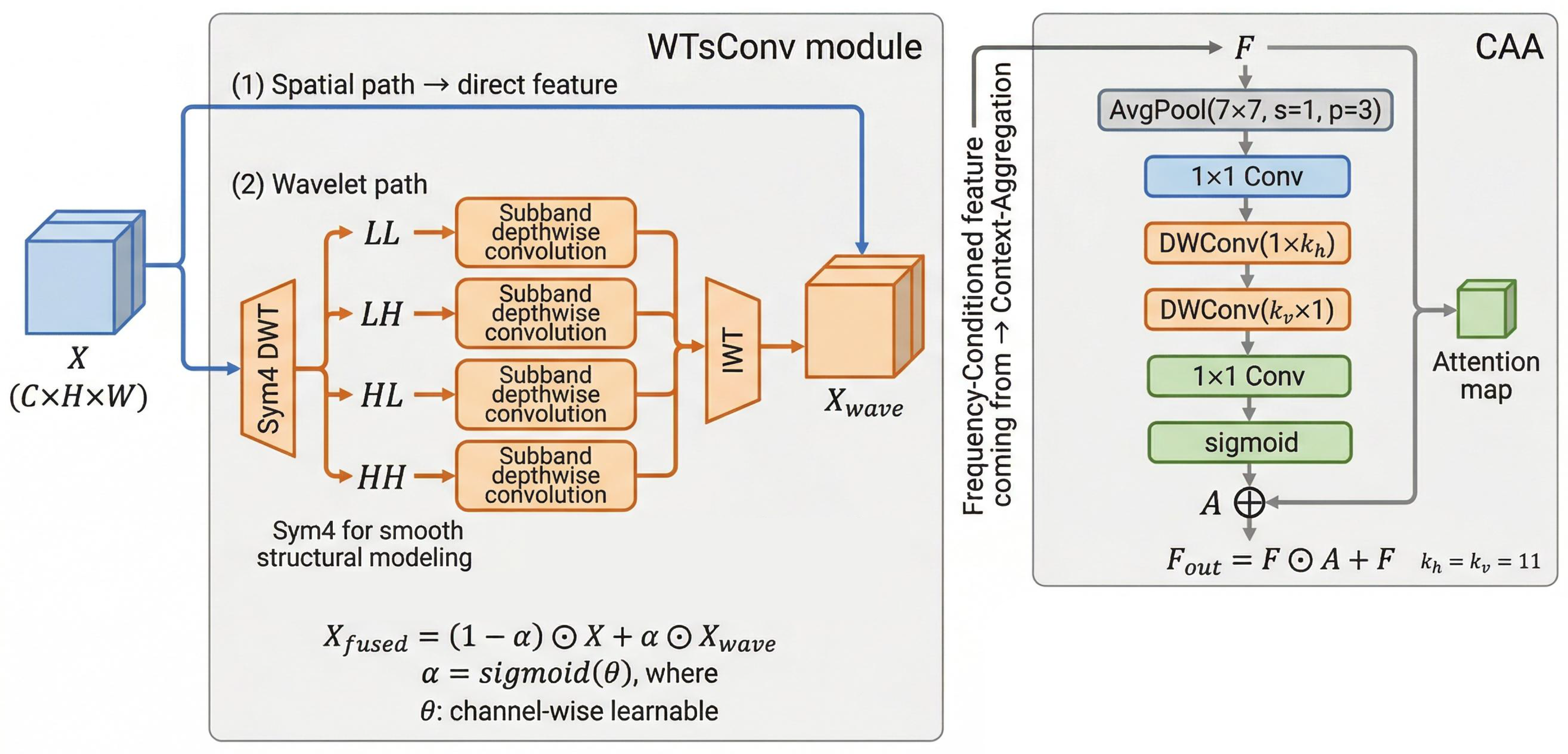
Detailed architecture of the proposed WTsConv module and CAA mechanism. Left (WTsConv): The input feature follows two parallel paths: (1) a direct spatial path preserving original features, and (2) a wavelet path performing Sym4-based DWT decomposition into four subbands (LL: low-low frequency, LH: low–high frequency, HL: high–low frequency, HH: high–high frequency), followed by subband-wise depthwise convolutions and IWT reconstruction to obtain . The two paths are fused via a learnable channel-wise weight to produce , where ⊙ denotes element-wise multiplication. Right (CAA): The contextual anchor attention module takes the frequency-conditioned feature as input, applies average pooling (, stride = 1, padding = 3), followed by two convolutions and two directional depthwise convolutions ( and , where ) to generate the attention map . The output applies residual modulation: . This cascaded design enables frequency-aware feature refinement followed by context-aware attention aggregation.
Figure 2.
Detailed architecture of the proposed WTsConv module and CAA mechanism. Left (WTsConv): The input feature follows two parallel paths: (1) a direct spatial path preserving original features, and (2) a wavelet path performing Sym4-based DWT decomposition into four subbands (LL: low-low frequency, LH: low–high frequency, HL: high–low frequency, HH: high–high frequency), followed by subband-wise depthwise convolutions and IWT reconstruction to obtain . The two paths are fused via a learnable channel-wise weight to produce , where ⊙ denotes element-wise multiplication. Right (CAA): The contextual anchor attention module takes the frequency-conditioned feature as input, applies average pooling (, stride = 1, padding = 3), followed by two convolutions and two directional depthwise convolutions ( and , where ) to generate the attention map . The output applies residual modulation: . This cascaded design enables frequency-aware feature refinement followed by context-aware attention aggregation.

Figure 3.
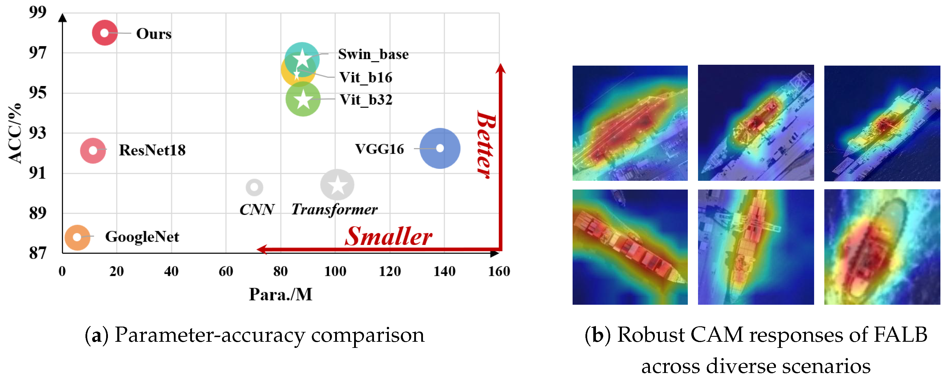
Comparison of parameter-accuracy trade-off and attention robustness: (a) FALB improves accuracy by 0.96% over ResNet50 while reducing parameters by 30.4% under the reported setting, achieving the optimal balance among compared baselines; (b) Grad-CAM visualizations of FALB across diverse and challenging maritime scenarios (including massive aircraft carriers, severe port clutter with gantry cranes, and intense high-speed wave wakes). The highly concentrated responses explicitly demonstrate that FALB consistently localizes intrinsic ship structures and effectively suppresses severe high-frequency background noise.
Figure 3.
Comparison of parameter-accuracy trade-off and attention robustness: (a) FALB improves accuracy by 0.96% over ResNet50 while reducing parameters by 30.4% under the reported setting, achieving the optimal balance among compared baselines; (b) Grad-CAM visualizations of FALB across diverse and challenging maritime scenarios (including massive aircraft carriers, severe port clutter with gantry cranes, and intense high-speed wave wakes). The highly concentrated responses explicitly demonstrate that FALB consistently localizes intrinsic ship structures and effectively suppresses severe high-frequency background noise.
Figure 4.
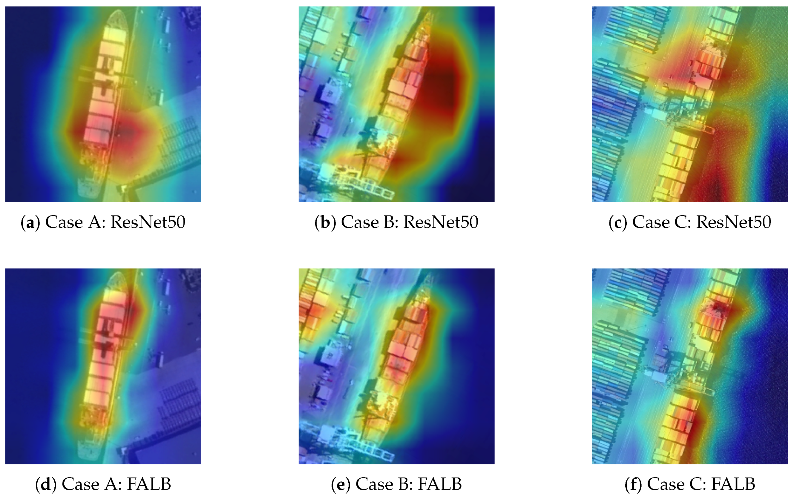
Additional paired Grad-CAM comparisons on three samples. (a–c): ResNet50; (d–f): FALB. Within each pair, both heatmaps are generated from the same input sample and target class under identical Grad-CAM settings.
Figure 4.
Additional paired Grad-CAM comparisons on three samples. (a–c): ResNet50; (d–f): FALB. Within each pair, both heatmaps are generated from the same input sample and target class under identical Grad-CAM settings.
Figure 5.
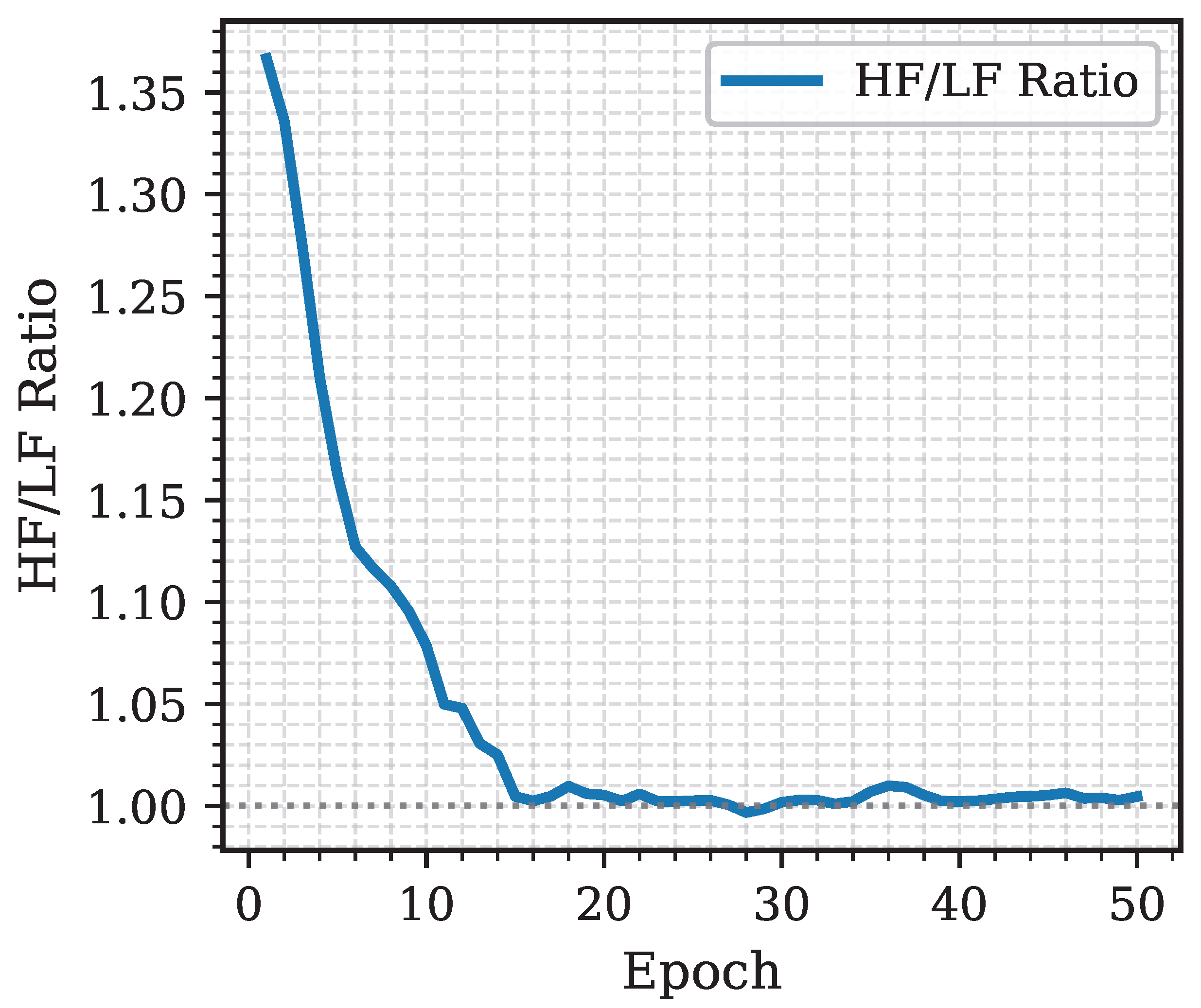
Epoch-wise evolution of the HF/LF ratio for a representative FALB run. The curve shows an early decrease followed by near-stable behavior around 1.00.
Figure 5.
Epoch-wise evolution of the HF/LF ratio for a representative FALB run. The curve shows an early decrease followed by near-stable behavior around 1.00.
Figure 6.
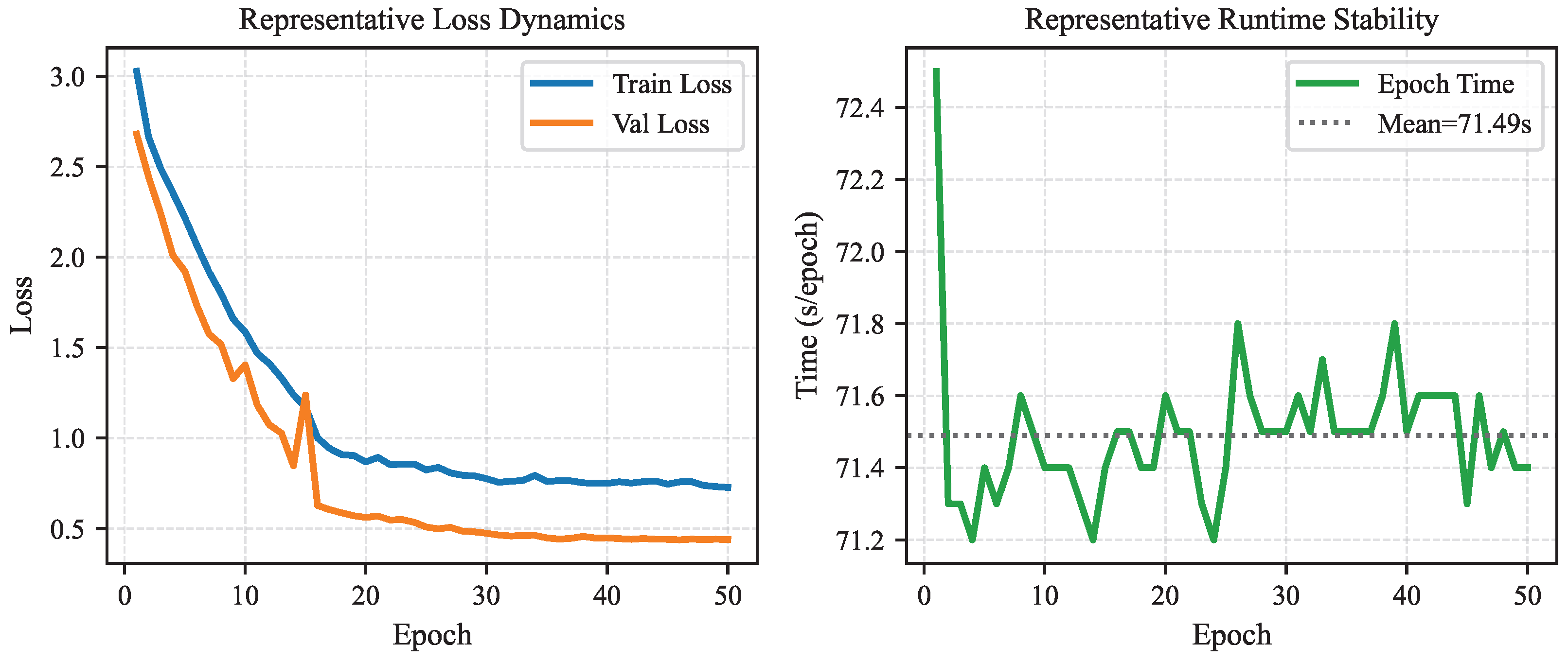
Representative optimization dynamics of a logged FALB run. (Left): training/validation loss trajectories over 50 epochs. (Right): epoch-wise runtime with mean-line reference.
Figure 6.
Representative optimization dynamics of a logged FALB run. (Left): training/validation loss trajectories over 50 epochs. (Right): epoch-wise runtime with mean-line reference.
Table 1.
Concise summary of representative families and remaining gaps for fine-grained ship classification.
Table 1.
Concise summary of representative families and remaining gaps for fine-grained ship classification.
| Family | Representative Works | Key Remaining Gap in Ship Classification |
|---|
| Spatial CNN backbones | ResNet, DenseNet, Xception, ConvNeXt, RepVGG [4,5,6,7,53] | Limited explicit frequency control under sea/dock clutter. |
| Mobile/lightweight CNNs | MobileNet series, ShuffleNet series, GhostNet, EfficientNet family [13,14,15,16,17,34,35,36] | Efficiency gains can come with weaker global structural cues in cluttered maritime backgrounds. |
| Attention and token-based models | Non-local/GC/ECA/CC attention, ViT/DeiT/PVT/Swin/PiT/ResMLP [19,20,21,22,44,45,46,47,54,55] | Attention on raw spatial features can still amplify irrelevant high-frequency background responses. |
| Frequency-aware designs | FcaNet, WaveCNet, WTConv, recent wavelet-enhanced remote sensing models [30,40,41,42,43] | The ordering between frequency refinement and context aggregation is often underexplored in lightweight bottlenecks. |
| Remote sensing ship-oriented methods | Feature-fusion and prompt-tuning pipelines with dedicated benchmarks [27,28,29,32,56] | Limited unified analysis of frequency-aware lightweight bottleneck design under strict complexity constraints. |
Table 2.
Comparison of accuracy and parameter count between FALB and state-of-the-art methods on FGSCM-52 dataset.
Table 2.
Comparison of accuracy and parameter count between FALB and state-of-the-art methods on FGSCM-52 dataset.
| Model | Type | Para. | ACC |
|---|
| ResNet18 [6] | CNN | 11.2 M | 92.12% |
| VGG16 [3] | CNN | 138.35 M | 92.23% |
| GoogLeNetv4 [57] | CNN | 5.64 M | 87.79% |
| Mobilenetv3-large [15] | CNN | 5.48 M | 93.21% |
| Efficientnet-b0 [16] | CNN | 5.29 M | 92.18% |
| ViT-b16 [19] | Transformer | 86.57 M | 96.18% |
| ViT-b32 [19] | Transformer | 88.22 M | 94.7% |
| Swin-base [21] | Transformer | 87.77 M | 96.66% |
| ResNet50 [6] | CNN | 25.56 M | 96.92% |
| ResNet50-WTConv [30] | CNN | 15.56 M | 96.81% |
| ResNet50-FALB | CNN | 17.78 M | 97.88% |
Table 3.
Derived efficiency indicators on FGSCM-52 from reported accuracy and parameter results.
Table 3.
Derived efficiency indicators on FGSCM-52 from reported accuracy and parameter results.
| Model | Para. (M) | ACC (%) | ACC/M | FP32 Size (MB) |
|---|
| ResNet50 | 25.56 | 96.92 | 3.79 | 102.24 |
| ResNet50-WTConv | 15.56 | 96.81 | 6.22 | 62.24 |
| ResNet50-FALB | 17.78 | 97.88 | 5.51 | 71.12 |
Table 4.
Comprehensive ablation study on FGSCM-52 showing the isolated and combined effects of each component.
Table 4.
Comprehensive ablation study on FGSCM-52 showing the isolated and combined effects of each component.
| CAA | WTConv | WTsConv | Para. | ACC (%) |
|---|
| - | - | - | 25.56 M | 96.92 |
| ✓ | - | - | 27.02 M | 96.11 |
| - | ✓ | - | 15.56 M | 96.81 |
| ✓ | ✓ | - | 17.02 M | 97.12 |
| - | - | ✓ | 16.32 M | 97.13 * |
| ✓ | - | ✓ | 17.78 M | 97.88 |
Table 5.
Training configuration summary used in the reported experiments.
Table 5.
Training configuration summary used in the reported experiments.
| Item | Setting |
|---|
| Input preprocessing | Training: RandomResizedCrop(224) + horizontal flip + ColorJitter(0.2,0.2,0.2,0.1); Val: Resize(256) + CenterCrop(224) |
| Optimizer and loss | SGD (momentum , weight decay ), cross-entropy |
| Learning rate schedule | Initial LR ; StepLR (step size 15, decay factor ) |
| Training duration | 50 epochs, batch size 32, 4 workers |
| Initialization protocol | Main comparisons: ImageNet pre-trained initialization; added cross-dataset wavelet/fusion analyses on FGSCR-42 also use ImageNet pre-trained initialization |
| Reproducibility control | SEED = 42 with deterministic cuDNN setting |
Table 6.
Runtime environment summary for reproducibility and profiling.
Table 6.
Runtime environment summary for reproducibility and profiling.
| Item | Setting |
|---|
| GPU setup | NVIDIA GeForce RTX 3080 |
| GPU driver | NVIDIA driver 566.24 |
| Operating system | Ubuntu 20.04 LTS |
| Python environment | Python 3.10.0 (Conda) |
| Deep learning framework | PyTorch 1.13.1+cu117 |
| CUDA/cuDNN runtime | CUDA 11.7, cuDNN 8.5 |
| Complexity tool | profile_complexity.py (FLOPs defined as 2 × MACs) |
Table 7.
Complexity profiling protocol details used for
Table 8.
Table 7.
Complexity profiling protocol details used for
Table 8.
| Item | Setting |
|---|
| Input tensor | |
| Execution mode | eval() + torch.inference_mode() |
| Operator coverage | Convolution/transpose-convolution/linear operations counted in both module and functional paths |
| Metric definition | MACs accumulated from counted operators; FLOPs reported as 2 × MACs |
| Comparison scope | Relative complexity comparison under identical script and input protocol |
Table 8.
Script-level compute profile under fixed protocol (, batch size 1, CUDA).
Table 8.
Script-level compute profile under fixed protocol (, batch size 1, CUDA).
| Model Variant | MACs (G) | FLOPs (G) |
|---|
| ResNet50 | 4.089 | 8.178 |
| ResNet50-WTConv | 2.792 | 5.584 |
| ResNet50-FALB | 3.317 | 6.634 |
Table 9.
Fusion strategy ablation on FGSCR-42 (ImageNet pre-training, 50 epochs, seeds = {42, 2026}).
Table 9.
Fusion strategy ablation on FGSCR-42 (ImageNet pre-training, 50 epochs, seeds = {42, 2026}).
| Fusion Strategy | ACC (%) | Std (%) |
|---|
| Symmetric (sym) | 96.40 | 0.61 |
| Gate | 97.21 | 0.75 |
| Decoupled (decouple) | 97.93 | 1.20 |
Table 10.
Derived optimization statistics from a representative logged FALB run.
Table 10.
Derived optimization statistics from a representative logged FALB run.
| Metric | Start | End/Aggregate |
|---|
| Training loss | 3.0273 (epoch 1) | 0.7270 (epoch 50) |
| Validation loss | 2.6801 (epoch 1) | 0.4394 (epoch 50) |
| HF/LF ratio | 1.3875 (epoch 1) | 1.0031 (epoch 50) |
| Epoch runtime | – | 71.49 s (mean) |
| Total wall-clock time | – | 59.58 min (50 epochs) |
Table 11.
Controlled wavelet-basis comparison in FALB on FGSCR-42 with ImageNet pretraining (50 epochs, seeds = {42, 2026}).
Table 11.
Controlled wavelet-basis comparison in FALB on FGSCR-42 with ImageNet pretraining (50 epochs, seeds = {42, 2026}).
| Wavelet Basis | Mean ACC | Std |
|---|
| Haar | 95.20% | 0.73 |
| Db4 | 92.47% | 1.10 |
| Sym4 | 96.40% | 0.61 |
Table 12.
Spectral energy distribution statistics on FGSCM-52 validation set (100 samples, DWT level = 2).
Table 12.
Spectral energy distribution statistics on FGSCM-52 validation set (100 samples, DWT level = 2).
| Wavelet | Ship Low (%) | Ship High (%) | BG Low (%) | BG High (%) |
|---|
| Haar | 94.65 ± 2.31 | 5.35 ± 2.31 | 83.41 ± 4.12 | 16.59 ± 4.12 |
| Db4 | 95.95 ± 1.87 | 4.05 ± 1.87 | 84.62 ± 3.95 | 15.38 ± 3.95 |
| Sym4 | 96.00 ± 1.82 | 4.00 ± 1.82 | 84.44 ± 3.88 | 15.56 ± 3.88 |
Table 13.
Frequency filter sensitivity experiments on FGSCR-42 (trained models, no retraining, seeds = {42, 2026}).
Table 13.
Frequency filter sensitivity experiments on FGSCR-42 (trained models, no retraining, seeds = {42, 2026}).
| Wavelet | Clean | Low pass (0.20) | High pass (0.20) | Bandstop (0.10–0.35) |
|---|
| Db4 | 92.47 | 34.90 | 2.53 | 35.75 |
| Haar | 95.20 | 37.80 | 6.07 | 38.44 |
| Sym4 | 96.40 | 37.99 | 4.39 | 33.41 |
Table 14.
CAA architecture optimization on FGSCR-42 (ImageNet pre-training, 50 epochs, seeds = {42, 2026}).
Table 14.
CAA architecture optimization on FGSCR-42 (ImageNet pre-training, 50 epochs, seeds = {42, 2026}).
| Variant | ACC (%) | Std (%) |
|---|
| ResNet-50 baseline | 92.31 | 0.23 |
| CAA-only (k = 7, BN) | 93.15 | 0.18 |
| CAA-only (k = 7, None) | 93.22 | 0.21 |
| CAA-only (k = 11, BN) | 93.48 | 0.15 |
| CAA-only (k = 11, None) | 93.31 | 0.19 |
| CAA-only (k = 15, BN) | 93.25 | 0.24 |
| CAA-only (k = 15, None) | 93.08 | 0.27 |
| FALB (WTsConv + CAA) | 96.40 | 0.61 |