


Highlights
What are the main findings?
- A transparent 2D feature space framework was developed to integrate polarimetric scattering components with optical salinity or vegetation indicators for oasis soil salinity monitoring.
- The multi-source VanZyl_vol–SI4 model achieved the best performance (fitting: R2 = 0.749; validation: R2 = 0.716), outperforming single-source feature space alternatives.
What are the implications of the main findings?
- Integrating physically based PolSAR scattering information with spectral indices can mitigate spectral saturation and surface heterogeneity effects, improving robustness in arid saline soils.
- The proposed 2D feature space design offers an interpretable pathway for operational monitoring of salt-affected soils to support management in arid oases.
Abstract
Soil salinization in arid oases constrains soil functioning and crop production, making spatially explicit monitoring important for land management. Multispectral optical remote sensing enables large-area salinity assessment, but in oasis environments such as the Keriya Oasis, its performance can be limited by spectral confusion between salt crusts and bright bare soils, sparse vegetation cover, and strong surface heterogeneity. Synthetic aperture radar (SAR), by contrast, provides all-weather imaging capability and sensitivity to surface scattering and dielectric-related conditions, but its salinity interpretation is often affected by surface complexity and environmental coupling. To address these, a spectral index–polarimetric scattering integration framework that combines RADARSAT-2 and Landsat-8 OLI features within a simple two-dimensional (2D) feature space was developed. Two groups of models were constructed from variables selected through a data-driven screening process: (1) polarimetric feature space models based on combinations such as VanZyl volume scattering with Pauli odd-bounce or Touzi alpha scattering; and (2) multi-source feature space models that integrate the optimal polarimetric component with key spectral indicators such as SI4 and MSAVI. Among all tested models, VanZyl_vol-SI4 achieved the best performance (fitting: R2 = 0.749, RMSE = 5.798 dS m−1, MAE = 4.086 dS m−1; validation: R2 = 0.716, RMSE = 5.566 dS m−1, MAE = 4.528 dS m−1). The results indicate that integrating PolSAR scattering information with optical indices can improve salinity mapping relative to single-source feature spaces in the Keriya Oasis. The proposed 2D framework provides a concise way to compare different feature combinations and supports regional identification of salt-affected soils.
1. Introduction
Soil salinization, a widespread form of land degradation, presents a significant challenge to agricultural productivity and ecological stability, threatening food security and ecosystem resilience globally [1]. According to the Food and Agriculture Organization (FAO) and recent global assessments, approximately 20 percent of irrigated land is salt-affected [2], and this issue is expected to worsen as climatic conditions evolve [3]. In arid environments, insufficient precipitation limits the leaching of salts from the root zone, while high evapotranspiration rates facilitate the upward movement of saline groundwater [4,5]. This phenomenon is particularly prominent in agricultural oases, intensive farming zones within arid landscapes dependent on irrigation, such as Northwest China, where increasing soil salinity results in significant annual yield reductions for essential crops, thereby affecting regional economic stability [6]. In light of these complexities, and given the spatial heterogeneity and temporal variability of soil salinization, there is a growing need for advanced monitoring systems that provide accurate, timely, and large-scale assessments to support effective remediation and sustainable land management.
Traditional salinity assessment relies on field sampling and laboratory measurement of soil electrical conductivity (EC), which provides reliable point-scale information but is labor-intensive and spatially limited [4]. Electromagnetic induction (EMI) can improve field-scale efficiency, yet its applicability remains constrained in large or logistically difficult areas [7,8]. Satellite remote sensing, therefore, offers an important alternative for synoptic salinity monitoring. [9]. Optical sensors such as Landsat and Sentinel-2 are sensitive to salt crusts, soil brightness, and vegetation stress, and have supported the development of salinity and vegetation indices for large-area mapping [7,10,11]. However, optical observations are affected by atmospheric conditions and mainly capture surface reflectance [12,13,14]. By contrast, synthetic aperture radar (SAR) provides complementary information related to surface structure and dielectric properties and can operate under cloud-affected conditions [15,16]. As soil salinity increases, EC rises and alters the complex dielectric constant, which can increase microwave attenuation and affect backscatter [12]. This alteration modulates the amount of microwave energy backscattered to the sensor, thereby establishing a physical basis for salinity estimation [17]. Additionally, longer-wavelength radar signals can partially penetrate dry soil surfaces, enabling the detection of subsurface salinity features that are not accessible to optical sensors [18]. Fully polarimetric SAR (PolSAR) further enriches this capability by capturing scattering information in multiple polarization channels, enabling polarimetric decomposition techniques that separate the total backscatter into components associated with distinct physical scattering mechanisms [18,19]. Such decomposition has the potential to enhance sensitivity to subtle salinity-related variations and to disentangle confounding effects (e.g., surface roughness and moisture) through mechanism-informed features.
Applying single-source remote sensing in the Keriya Oasis remains challenging because this oasis–desert ecotone exhibits strong regional heterogeneity [20]. The landscape is characterized by sparse vegetation, mosaic distributions of salt crusts and bright bare soils, strong short-range surface variability, and spatially variable shallow groundwater influence [19]. Under these conditions, optical observations may confuse highly reflective salt-encrusted surfaces with non-saline bright bare soils, especially where vegetation cover is discontinuous [18]. Meanwhile, although C-band PolSAR provides valuable structural and near-surface dielectric information, its response can also be influenced by shallow soil moisture fluctuations and micro-topographic roughness [20,21]. These regional ambiguities indicate that neither optical nor radar observations alone can straightforwardly characterize salinity gradients in this environment, thereby motivating an integrated framework that combines optical spectral response with polarimetric scattering information for salinity monitoring in the Keriya Oasis.
Feature space analysis has become an important framework for integrating remote sensing variables for salinity-oriented interpretation [22,23,24]. Early applications mainly relied on optical feature pairs to characterize land degradation and salinity gradients in arid environments [25,26,27]. Subsequently, the framework was extended to radar-related studies, and PolSAR-derived feature spaces were shown to capture salinity-related variations from the perspective of scattering behavior [28,29]. In parallel, recent salinity monitoring studies have also developed along broader multi-source directions, including machine learning-based radar–optical estimation and other higher-dimensional fusion strategies [20,21,30]. These approaches have improved predictive flexibility, but their internal feature interactions are often less directly interpretable. In this context, a two-dimensional (2D) feature space remains a useful alternative because it preserves a clear geometric structure, supports direct pairwise comparison between radar and optical variables, and facilitates intuitive description of salinity gradients [31].
Despite this progress, several issues remain insufficiently addressed for PolSAR-optical salinity monitoring in heterogeneous arid oases. First, previous feature space studies have demonstrated the usefulness of radar- or optical-based pairings, but systematic comparison among polarimetric components representing different scattering categories remains limited [29,31,32]. Second, in cross-source 2D feature spaces, the optical variable is still often selected from a relatively restricted set of conventional indices, whereas broader data-guided screening may better identify variables suited to heterogeneous conditions involving salinity, bare soil, and sparse vegetation [31,33]. Third, although recent multi-source methods can enhance predictive performance [18,20,34], they do not fully address a different methodological question considered here: which optical descriptor most effectively complements a selected polarimetric scattering component when clear geometric interpretation is retained within a simple 2D framework?
Against this background, this study aims to enhance soil salinity monitoring in the Keriya Oasis by developing refined 2D feature space models using RADARSAT-2 and Landsat-8 OLI data. Specifically, we (1) construct and compare polarimetric feature space models using components that represent different scattering mechanisms, (2) develop multi-source feature space models by integrating the selected polarimetric feature with data-screened optical variables, and (3) evaluate the inversion performance of these configurations against independent validation data to identify the most effective feature space model for regional salinity assessment.
2. Materials and Methods
2.1. Study Area Description
This study focuses on the Keriya Oasis, located in the Hotan Region of Xinjiang, China (Figure 1). The oasis, part of the Keriya River basin, is geographically positioned between the southern edge of the Taklamakan Desert and the northern slopes of the Kunlun Mountains [35], spanning 36°30′–37°05″N latitude and 81°09′–82°03″E longitude [18]. Covering approximately 40,000 km2, the area exhibits a general north–south elevation gradient [19]. The region is characterized by a typical arid continental climate, with an average annual temperature of 12.2 °C, low annual precipitation, and high potential evaporation [19]. Soils are inherently alkaline and saline, while natural vegetation is sparse and dominated by desert-adapted species such as reeds and tamarisks [36].
Figure 1.
Overview of the study area. (a) imagery coverage area with sample points in this study; (b) RADARSAT-2 imagery; (c) Landsat-8 OLI imagery, and (d–h) are the landscapes of the study area.
The Keriya Oasis also represents a complex salinity-monitoring environment from both environmental and remote sensing perspectives [18]. At the oasis scale, salinity patterns are jointly influenced by strong evaporation, spatially variable shallow groundwater conditions, imperfect drainage in marginal and lower-lying zones, and contrasting irrigation leaching conditions between cultivated land and desert-fringe areas [19]. As a result, salt accumulation is spatially heterogeneous, with stronger surface expression typically occurring in marginal and terminal zones, where salt-affected surfaces are mainly manifested as bare saline soils and surface salt crusts. Together with the coexistence of cultivated patches, bare soils, and sparsely vegetated zones, these conditions generate substantial heterogeneity in land-surface reflectance and scattering behavior [37]. These diverse and challenging environmental conditions provide a representative setting for the development and validation of multi-sensor monitoring strategies. Figure 1a further shows the local study area used in this work, including the image-covered analysis extent and the spatial distribution of field sampling points.
2.2. Data Acquisition and Pre-Processing
The overall methodological framework of this study is presented in Figure 2.
Figure 2.
The workflow of the study. In the figure, EC is soil electrical conductivity. The “*” is p < 0.05, and “ns” is not significant.
2.2.1. PolSAR-Optical Remote Sensing Data
To develop an integrated monitoring approach, both active microwave and passive optical remote sensing data were employed. The microwave dataset consisted of a RADARSAT-2 fully PolSAR image (Level 1.1, C-band, 5.4 GHz, right-looking, descending orbit, 41.05° incidence angle, spatial resolution 5.5 m × 4.8 m in range and azimuth, quad polarization modes including HH, HV, VH, and VV), acquired on 6 May 2022. The optical dataset consisted of a Landsat-8 Operational Land Imager (OLI) scene, acquired on 15 May 2022, which provides 11 spectral bands at 30 m spatial resolution and a 16-day revisit cycle, with less than 12% cloud cover. Landsat-8 OLI is a well-established data source for land surface monitoring, including soil salinity assessments [38]. The close temporal proximity of these acquisitions to the field campaign ensured that the remote sensing data accurately represented ground conditions.
A systematic pre-processing workflow was implemented to correct for sensor and atmospheric distortions and prepare the data for synergistic analysis. For the Landsat-8 OLI Level-1T product, standard geometric and terrain corrections were supplemented by radiometric calibration (to surface reflectance) and atmospheric correction (FLAASH module) in ENVI® 5.4. The imagery was resampled to a 10 m × 10 m pixel size to match the analysis scale, followed by projection transformation and clipping to the study area boundary. For the RADARSAT-2 data, ESA SNAP® 9.0 was used for radiometric calibration, generation of the 3 × 3 polarimetric coherency matrix (T3), multi-looking, geocoding, speckle filtering, and polarimetric decomposition. Subsequent projection transformation and precise geometric co-registration with the optical data were conducted in ENVI® 5.4 to ensure accurate spatial alignment.
2.2.2. Field Data Collection and Laboratory Analysis
A field campaign was conducted from 1 to 13 May 2022 to collect ground-truth soil samples. This period was chosen as it represents a phase of relatively stable soil salinity, following winter salt accumulation and preceding summer irrigation-induced leaching, and coincides with the critical crop germination stage. A stratified random sampling strategy was applied to ensure representative coverage of the oasis core, agricultural–desert transition zone, and desert fringe. Site selection was informed by Ovitalmap®, topographic maps, and land use classifications. Within the RADARSAT-2 image footprint, 80 primary sampling sites were established. At each site, a five-point composite sample (≈500 g) was collected from the topsoil layer (0–10 cm) within a 10 m × 10 m grid, consistent with the resampled remote sensing data resolution [39]. The geographic coordinates of each site were recorded using a high-precision GPS (±1 m accuracy), and ancillary information on local vegetation and soil surface characteristics was documented.
In the laboratory, all soil samples were air-dried, mechanically ground, and passed through a 2 mm sieve to remove coarse fragments. EC was measured using a soil-to-water mass ratio of 1:5 (EC 1:5); the suspension was agitated for 200 oscillations, settled for four hours, and vacuum-filtered at 25 °C. The EC of the filtrate was measured with a calibrated Mettler Toledo FE38 (Greifensee, Switzerland) conductivity meter. The EC 1:5 value served as the quantitative indicator of soil salinity for subsequent modeling, as it is a standard and reproducible proxy for salt concentration [12].
The measured EC values showed a broad distribution across the sampled sites. For the full dataset, EC ranged from 0.03 to 59.58 dS m−1, with a median of 4.365 dS m−1. The fitting subset covered a comparable range, from 0.03 to 59.58 dS m−1, with a median of 4.40 dS m−1, while the validation subset ranged from 0.06 to 40.78 dS m−1, with a median of 4.33 dS m−1. According to the EC-based salinity classification of Abrol et al. (1988) [40], the full dataset covered the main salinity classes represented in the study area. The fitting and validation subsets retained comparable class coverage (Table S1), supporting their use for model calibration and independent validation under the present sampling design. The EC distributions of the full, fitting, and validation datasets are further illustrated in Figure 3.
Figure 3.
EC distributions for the full dataset, fitting subset, and validation subset.
2.3. Polarimetric Decomposition for Feature Extraction
PolSAR data provides a complete description of the scattering process through the 2 × 2 Sinclair scattering matrix [S], which relates the scattered and incident electromagnetic fields [41,42]. To transform this complex data into physically meaningful variables, target decomposition techniques are employed [42]. In this study, both coherent target decomposition (CTD) and incoherent (ITD) were considered. CTD operates directly on the scattering matrix and was represented here by the Pauli decomposition [43,44], which separates the response into odd-bounce, even-bounce, and ±45°-oriented components [44,45,46]. For distributed natural targets, ITD methods use second-order descriptors, mainly the covariance matrix [C] and coherency matrix [T], to decompose the measured polarimetric response into canonical scattering components with clearer physical meaning (Figure 4) [41,47,48,49].
Figure 4.
The different scattering characteristics of SAR signals.
Following previous studies, the extracted polarimetric features were not compared simply by their parent decomposition algorithms, but were reorganized according to the physical scattering mechanisms they primarily represent. The candidate features were therefore grouped into five categories: surface scattering, double-bounce scattering, volume scattering, helix scattering, and statistical/geometric descriptors (Table 1). This physically based regrouping provides a more direct basis for comparing how different scattering responses relate to soil salinity. The full list of decomposition components used in this study is provided in Appendix A (Table A1).
Table 1.
Polarimetric feature components grouped by physical scattering mechanism.
2.4. Derivation of Candidate Spectral Indicators
Soil salinization in arid regions such as the Keriya Oasis can be expressed optically through two main pathways: (1) direct spectral responses of salt-affected bare soil and salt crusts; and (2) indirect vegetation responses caused by salinity stress [56,57]. Based on this understanding, 45 optical indices widely used in salinity-related remote sensing studies were selected as candidate variables for further analysis. The candidate set was organized into two groups, including 25 optical salinity indices and 20 optical vegetation indices. The first group was intended to characterize direct spectral responses of saline surfaces [4,10,58], whereas the second group was designed to capture indirect salinity signals through vegetation condition and stress response [59,60]. This grouped design was adopted to ensure that both bare soil- and vegetation-mediated salinity information could be represented under the heterogeneous oasis conditions of the study area. Details and formulas of these indices are provided in Tables S2 and S3 of the Supplementary Materials.
2.5. Optimal Feature Selection
2.5.1. Selection of the Optimal PolSAR Feature Component
Polarimetric decompositions produce numerous feature components, each exhibiting distinct sensitivities to soil properties and varying levels of signal quality [29]. To identify the most informative PolSAR features, we implemented a two-stage selection strategy emphasizing both signal fidelity and predictive relevance.
Stage 1: Signal-to-Noise Ratio (SNR) Screening. To ensure data quality, we calculated the SNR for each component within the five scattering mechanism groups (Table S4 in Supplementary Materials). From each group, the two components with the highest SNR were selected, resulting in a candidate pool of 10 features (Figure 5). This pre-screening step excluded noise-prone components, ensuring that only features with high signal integrity advanced to the next stage.
Figure 5.
The SNR value of polarimetric components (dB). Red labels indicate the components selected for further analysis.
Stage 2: Random Forest (RF) Importance Ranking. The 10 high-SNR candidates were then evaluated for their predictive relevance to soil EC using the RF algorithm. This step was introduced to provide an objective and unified importance criterion for further optimizing the retained candidate components before feature space construction. RF-based variable ranking has been widely used in remote sensing studies for parameter optimization because it can evaluate the relative contribution of candidate predictors under complex predictor-response relationships [33,61,62]. In this study, feature ranking was implemented in R(v4.2.2) using the randomForest (v4.7-1.2) and rfPermute (v2.5.2) packages. Variable importance was evaluated by the percent increase in mean squared error (%IncMSE). Statistical significance of importance scores was assessed by response-permutation testing using rfPermute (nrep = 500). The final RF ranking was run with ntree = 500 under set.seed (123), and mtry was not manually specified, so the default regression setting of the randomForest package was used. As shown in Figure 6, VanZyl_vol, Pauli_odd, and Touzi_alpha exhibited the highest importance and were statistically significant (p < 0.05).
Figure 6.
Importance of polarimetric feature components calculated by the Random Forest (RF) algorithm. The “*” is p < 0.05, and “ns” is not significant.
2.5.2. Selection of the Optimal Spectral Indices
To construct the most effective multi-source feature space, the optimal PolSAR feature was paired with an optical index that provides complementary information. As described in Section 2.4, the optical candidate set was organized into two groups representing two salinity-related optical pathways: direct saline surface response and indirect vegetation stress response. To assess which type of optical information provides greater complementarity to the selected PolSAR feature, a comparative feature evaluation was performed [20]. This grouped screening procedure also helped limit the influence of redundancy among candidate indices constructed from similar band combinations, because representative variables were identified separately within each response pathway before subsequent multi-source integration [63].
Specifically, the same RF importance ranking framework was then applied separately to the two optical groups, so that optical variables were screened using a consistent importance criterion before subsequent multi-source pairing. Among the 25 soil-focused indices, Salinity Index 4 (SI4) exhibited the highest association with measured soil EC (Figure 7a), thereby representing the optimal indicator for direct soil spectral responses to salinity. For the 20 vegetation-focused indices, Modified Soil Adjusted Vegetation Index (MSAVI) was ranked as the most significant (Figure 7b), highlighting its suitability for capturing the indirect vegetation stress response. In this way, the final optical screening did not retain the full candidate pool for subsequent model construction, but selected one representative index from each optical response group. This design improved the stability and interpretability of the final optical feature set used in the 2D multi-source feature space models.
Figure 7.
Importance of spectral indices calculated by the RF algorithm: (a) salinity indices; (b) vegetation indices. The “*” represents p < 0.05; “ns” is not significant.
2.6. Principle and Application of the Feature Space Method
Based on the selected feature set, feature space construction was then performed. Prior to this step, the selected features were linearly rescaled to the interval [0, 1] using Min–Max normalization to ensure comparability among variables with different original scales [32,64]. Expanding upon previous studies [27,28,64], our research systematically investigates two configurations: (1) PolSAR only feature spaces, constructed from scattering components representing distinct physical mechanisms; and (2) multi-source feature spaces, which integrate PolSAR and optical data to explore their complementary advantages. Based on the data-driven feature selection process, the following four feature pairs were chosen: (a) two 2D polarimetric feature spaces, and (b) two 2D multi-source feature spaces. For each feature pair, a feature space conceptualization was established to interpret how the joint variation in the two features corresponds to soil salinity conditions [28,32,65]. In this framework, each pixel is represented as a point in a 2D feature space defined by the selected feature pair.
As illustrated in Figure 8, this procedure is based on the Euclidean distance between each pixel’s coordinates in the feature space and a predefined ideal point. After normalization to [0, 1], this ideal point serves as the reference point in the feature space, and smaller distances indicate weaker salinity influence [29]. The general form of the distance calculation can be expressed as follows:
where denotes the feature space distance for pixel , and are the normalized coordinates of the pixel in the feature space, and and represent the coordinates of the ideal point. Similar reference state and distance- or boundary-based formulations have been adopted in related feature space studies. For example, Muhetaer et al. [29] used Point A (1, 1) as the reference point in a radar feature space for soil salinity in the Keriya Oasis and characterized the salinization degree from the distance between any point in the feature space and that reference point. Guo et al. [33] likewise described a point-to-point salinity feature space model in which the distance from any point to O (1, 0) was used to distinguish different salinity levels. He et al. [31] similarly constructed several 2D salinity feature spaces using normalized parameters and derived salinity-related indices from the distance to a reference point such as (1, 0). Following this line of work, the ideal point in this study was defined within the normalized feature space as the reference state for subsequent feature space distance calculation.
Figure 8.
Conceptual diagram of the feature space model. The “ideal point” corresponds to reference conditions.
3. Results
3.1. Establishment of a Two-Dimensional Feature Space Model for Salinity Monitoring
3.1.1. Design of Polarimetric Feature Space Models for Soil Salinity Characterization
The two polarimetric feature space models were designed to leverage the unique sensitivity of polarimetric parameters to vegetation and soil surface properties. The first space combines the volume scattering component (VanZyl_vol) with a surface dominant scattering component (Pauli_odd) (Figure 9a). VanZyl_vol is commonly associated with scattering from vegetation canopies or other randomly oriented elements [66,67], whereas Pauli_odd captures the intensity of odd-bounce scattering and is sensitive to near-surface conditions [20,46,51].
Figure 9.
Scatter plots of the polarimetric feature spaces: (a) VanZyl_vol-Pauli_odd; (b) VanZyl_vol-Touzi_alpha.
The second model pairs the VanZyl_vol component with the Touzi_alpha component (Figure 9b). Rather than directly characterizing salinity gradients, this space is designed to reduce confounding responses, particularly strong double-bounce scattering from built-up areas. Touzi_alpha is sensitive to scattering mechanism differences and thus supports land-cover discrimination [49,53].
As shown in Figure 9, both feature spaces exhibit an approximately linear trend between the paired components, suggesting their potential for discriminating soils with varying salinization levels. Taking the VanZyl_vol-Pauli_odd feature space as an example (Figure 10), scatter points associated with different salinization levels occupy different parts of the feature space and show a salinity-related gradient along the dominant trend. The non-saline areas (green) concentrate toward the upper-right portion of the distribution, indicative of relatively healthy vegetation and weak salinity influence, whereas slightly to heavily salinized soils progressively shift toward the lower-left region, corresponding to reduced vegetation cover and altered soil surface conditions. This is consistent with the findings of Nurmemet et al. [28], who demonstrated the utility of volume scattering for mapping salinity gradients. This observed segregation of salinity classes forms the conceptual basis for the proposed monitoring models. Within this framework, the position of a pixel’s data point along the dominant trend of the feature space distribution provides the basis for the subsequent feature space distance calculation and salinity characterization. To provide statistical support for the observed salinity-related separation, class-wise descriptive statistics of the normalized VanZyl_vol and Pauli_odd coordinates were further calculated for the four salinity groups, together with one-way ANOVA (Tables S5 and S7). The results showed significant among-group differences, supporting the observed gradient-based differentiation in the VanZyl_vol-Pauli_odd feature space.
Figure 10.
Distribution of soil salinization levels within the VanZyl_vol-Pauli_odd feature space. The color gradient from green (non-salinized) to red (heavily salinized) follows the dominant trend, supporting the use of pixel position for salinity characterization.
3.1.2. Integration of PolSAR and Multispectral Data in Multi-Source Feature Space Models
As shown in Figure 11a, the first multi-source feature space combines the VanZyl_vol component with the SI4 index. The underlying model for this space is based on an inverse relationship: declining vegetation structure and associated volume scattering contribution (lower VanZyl_vol) corresponds to stronger spectral evidence of surface salinity (higher SI4).
Figure 11.
Scatter plot of multi-source feature spaces: (a) VanZyl_vol-SI4; (b) VanZyl_vol-MSAVI.
The second multi-source feature space combines VanZyl_vol with MSAVI. This model reflects salinity-induced vegetation stress through two related aspects of vegetation condition: structure (VanZyl_vol) and greenness (MSAVI). Unlike SI4, MSAVI is designed to enhance vegetation signal while reducing soil background effects [68]. The VanZyl_vol-MSAVI space shows an overall positive association between the two variables (Figure 11b), providing a vegetation-centric perspective on salinity impacts, complementing the soil-focused VanZyl_vol-SI4 model.
Taking VanZyl_vol-SI4 as an example (Figure 12), different salinization levels exhibit a clear distribution pattern. Non-salinized vegetated areas (green) are concentrated at high VanZyl_vol and low SI4 values. With increasing salinity, vegetation condition declines and surface salt signals become more apparent: slightly salinized soils (yellow) shift toward lower VanZyl_vol and higher SI4, and this trend continues for moderately (purple) and heavily salinized soils (red), which occupy the region of lowest VanZyl_vol and highest SI4. This distribution supports the use of pixel position in the feature space for salinity characterization. A similar salinity-related differentiation was observed in the VanZyl_vol-SI4 feature space. Class-wise descriptive statistics of the normalized VanZyl_vol and SI4 coordinates, together with one-way ANOVA across the four salinity groups, also showed significant among-group differences (Tables S6 and S7), further supporting the observed gradient-based separation in Figure 12.
Figure 12.
Distribution of soil salinization levels within the VanZyl_vol-SI4 feature space, illustrating the negative trend (green: non-salinized; yellow: slightly salinized; purple: moderately salinized; red: heavily salinized).
3.2. Soil Salinity Mapping in Feature Space Framework
3.2.1. Feature Space Distance Calculation for Salinity Mapping
Following the feature space configurations established in Section 3.1, the corresponding feature space distances were calculated for the four selected models to support subsequent salinity mapping. For each feature space, the ideal reference point was assigned according to the directional meaning of the paired normalized features and the location of the lower-salinity end in the corresponding distribution. Accordingly, was used for the VanZyl_vol-Pauli_odd and VanZyl_vol-Touzi_alpha spaces, for the VanZyl_vol-SI4 space, and for the VanZyl_vol-MSAVI space. The specific reference-point settings and corresponding distance expressions are summarized in Table 2, and the schematic configurations are shown in Figure 13. Under this framework, larger distances indicate a greater deviation from the low-salinity reference state and thus stronger salinity influence.
Table 2.
Reference point settings and feature space distance expressions of the four selected models.
Figure 13.
Schematic configurations of feature space distance calculation for the models: (a) VanZyl_vol-Pauli_odd; (b) VanZyl_vol-Touzi_alpha; (c) VanZyl_vol-SI4; (d) VanZyl_vol-MSAVI.
3.2.2. Mapping Results
To map the spatial distribution of soil salinity across the Keriya Oasis, we applied four 2D feature space models and visualized the resulting salinity patterns (Figure 14). A consistent color gradient is used, where deep green indicates low salinity (favorable conditions) and progressively shifts through light green and yellow to deep orange, representing severe salinization. Visual comparison of the four maps reveals a broadly similar regional gradient: the lowest salinity levels are concentrated in the oasis core, whereas higher salinity levels occur predominantly in peripheral and low-lying areas. The four maps differ mainly in local continuity and fine-scale spatial detail [29].
Figure 14.
Spatial distribution of salinity severity in the Keriya Oasis: (a) VanZyl_vol-Pauli_odd; (b) VanZyl_vol-Touzi_alpha; (c) VanZyl_vol-SI4; and (d) VanZyl_vol-MSAVI. Colors indicate increasing salinization severity from low (deep green) to high (deep orange).
3.2.3. Comparison of Local Detail Visualization
To compare the ability of the models to represent fine-scale salinity patterns, a typical sub-region characterized by severe salinization was selected for close-up inspection (Figure 15). This local-scale analysis enables a comparison of how well the four feature space model outputs delineate salt-affected patterns relative to the Landsat-8 optical composite, where salt crusts appear as bright features. As shown in Figure 15e,f, the selected zoom-in area contains prominent salt crusts that correspond to the severe salinization zones (dashed ovals), supported by the field photograph (Figure 15g). The spatial patterns produced by the four models (Figure 15a–d) show visible differences in patch continuity, boundary delineation, and fine-scale spatial detail.
Figure 15.
Detailed spatial visualization. (a–d) Salinity patterns based on feature space models of VanZyl_vol-Pauli_odd, VanZyl_vol-Touzi_alpha, VanZyl_vol-SI4, and VanZyl_vol-MSAVI, respectively; (e) overview of the study area with the red box indicating the zoom-in location; (f) detailed view of the optical image (Landsat-8 true color) showing the distribution of severe salinization (dashed ovals); (g) field view of salt crusts.
Specifically, the polarimetric feature space models (Figure 15a,b) successfully identify the general high-salinity zones but show relatively fragmented patterns in some local areas. In contrast, the multi-source feature space models (Figure 15c,d) exhibit comparatively smoother patch continuity and clearer local boundaries.
3.3. Accuracy Assessment and Optimal Model Selection
3.3.1. Accuracy Assessment
To quantitatively evaluate the four 2D feature space models, we assessed their agreement with field-measured EC collected from the topsoil (0–10 cm). Among the 80 samples, 55 samples were used for model fitting, and the remaining 25 points were reserved for independent validation. Performance was summarized using the coefficient of determination (R2), Nash–Sutcliffe efficiency (NSE), mean absolute error (MAE), root mean square error (RMSE), and relative root mean square error (rRMSE) [20]. As shown in Table 3, in the fitting subset, the VanZyl_vol-SI4 model achieved the best performance (R2 = 0.749; NSE = 0.749; MAE = 4.086 dS m−1; RMSE = 5.798 dS m−1; rRMSE = 65%). On the validation subset, it remained the most accurate (R2 = 0.716; NSE = 0.716; MAE = 4.528 dS m−1; RMSE = 5.566 dS m−1; rRMSE = 63%), indicating more stable performance than the other feature space configurations under the same sampling design.
Table 3.
Accuracy statistics of four feature space models against field EC for the fitting subset (n = 55) and independent validation subset (n= 25).
For comparison, two single-variable baseline regressions based on SI4 alone and VanZyl_vol alone were also evaluated (Table S8). The SI4 only baseline yielded R2 = 0.358 for the fitting subset and R2 = 0.322 for the validation subset, whereas the VanZyl_vol only baseline yielded R2 = 0.350 and R2 = 0.230, respectively. Both baselines were weaker than the corresponding 2D feature space models, further indicating that the improved performance of the proposed models arises from the complementary use of paired variables rather than from either variable alone. The spatial distribution of absolute prediction errors for the validation samples is shown in Figure S1 as a visual reference for the location and magnitude of model errors under the present sampling design. Although the validation subset is limited in size for a highly heterogeneous salinity environment, it still provides an independent check on model generalization because the fitting/validation partition retained the main salinity classes represented in the study area.
3.3.2. Spatial Interpretation of the Optimal Model
Based on the optimal model, we mapped EC across the Keriya Oasis (Figure 16) and examined its spatial gradients using three representative subregions. The EC map shows a clear oasis-scale salinity pattern. High EC values (orange–red) concentrate along the oasis margins, especially in low-lying terminal flats toward the northern to northeastern periphery and in the southwestern margin. In contrast, low-EC zones occur mainly in (i) a distinct north–south corridor in the central–western part of the oasis following the main river–floodplain system, and (ii) relatively low-EC patches within cultivated blocks. Moderate EC levels (yellow–light green) dominate the transition between these end-members, forming broad transition belts between high- and low-EC areas. The zoom-ins (Figure 16c–h) suggest that EC contrasts in the predicted maps (Figure 16c,e,g) are broadly consistent with field-parcel patterns and land-cover transitions in the true-color imagery (Figure 16d,f,h), indicating fine-scale salinity heterogeneity.
Figure 16.
Spatial distribution of EC in the Keriya Oasis based on the optimal feature space model. (a) EC map; (b) true-color image; and paired subregion zoom-ins (c,d), (e,f), and (g,h), where (c,e,g) are predicted EC and (d,f,h) are the corresponding true-color images. Impervious surfaces are outlined.
4. Discussion
4.1. Advantages of Combining Complementary Scattering Mechanisms for Polarimetric Salinity Monitoring
Building on previous studies that demonstrated the utility of polarimetric SAR for salinity monitoring [20,28,63], this work extends feature space modeling by explicitly combining polarimetric descriptors sensitive to different land-surface components within a unified 2D framework. While prior research, such as Muhetaer et al. [29], effectively utilized features sensitive to volume scattering, our approach investigated the potential benefits of combining parameters sensitive to different components of the landscape: one primarily reflecting vegetation status and the other surface soil conditions.
Among the polarimetric configurations tested, the VanZyl_vol-Pauli_odd feature space model showed consistently stronger agreement with field EC than VanZyl_vol-Touzi_alpha. This result is consistent with the complementary sensitivity of the two selected variables to different salinity-related surface responses in the Keriya Oasis. VanZyl_vol represents the volume scattering contribution in the Van Zyl decomposition and is closely associated with vegetation structure and canopy condition [20,29,53]. Because the field campaign was conducted in early May, corresponding to the early growth stage, salinity stress can suppress vegetation vigor and canopy development, which may in turn weaken the corresponding volume scattering response [20,29,69], and also previous salinity studies in arid oases showing that volume scattering-related polarimetric components can contribute useful information for salinity discrimination [29]. In this sense, the relevance of VanZyl_vol in the present study lies in its ability to reflect vegetation-related structural variation under salinity influence, rather than only its statistical importance in feature ranking.
Pauli_odd, by contrast, captures the intensity of surface-dominant scattering and is influenced by near-surface dielectric contrast and surface roughness [20,46,51]. In severely salt-affected areas, salt crust formation and associated surface alteration can modify the physical condition and roughness of the exposed soil surface. Previous studies have also shown that salinity can influence the dielectric properties of geological materials, with implications for radar backscatter response under saline surface conditions [12]. These effects provide a plausible physical basis for the sensitivity of Pauli_odd to salinity-related surface change in the present study. Accordingly, the VanZyl_vol-Pauli_odd combination links two complementary salinity-related response domains: vegetation-related structural variation and near-surface scattering variation. This complementary design can reduce ambiguity inherent in single-feature interpretations. For example, low-volume scattering contribution may arise from salinity-induced vegetation degradation, but it may also occur in naturally bare or sparsely vegetated areas that are not necessarily saline. Introducing a surface-sensitive descriptor helps distinguish these cases by adding information on surface condition, thereby lowering the risk of misclassification when mapping salinity gradients across heterogeneous oasis landscapes.
This interpretation should also remain appropriately cautious. In dry desert farmland, C-band radar responses are still influenced by soil moisture and surface roughness, so salinity alone does not uniquely determine the backscatter behavior. For this reason, the selected polarimetric variables are discussed here as salinity-sensitive descriptors under coupled vegetation–surface conditions. A comparison with the VanZyl_vol-Touzi_alpha configuration further highlights the role of mechanism specificity. Touzi_alpha is intended to represent the dominant scattering mechanism (e.g., surface, volume, or double-bounce) and is therefore more “categorical” in nature [41,53,54], whereas Pauli_odd directly measures the intensity of surface-dominant scattering. The relatively better performance of VanZyl_vol-Pauli_odd suggests that, for this application, pairing a vegetation-related component with a direct surface-intensity proxy provides a more effective complement than pairing it with a generalized mechanism classification parameter. This complementary configuration is consistent with the direction of recent multi-parameter PolSAR salinity studies, where coupling vegetation- and surface-related scattering cues tends to yield more stable salinity discrimination than relying on a single scattering proxy [29,31].
4.2. Optimizing Multi-Source Fusion Through Data-Driven Feature Selection
Effective multi-source salinity monitoring relies not only on sensor complementarity but also on selecting non-redundant variables that capture distinct salinity-related mechanisms. In a 2D feature space framework, a key practical issue is determining which optical descriptor most effectively complements a radar-derived component while minimizing information overlap. To address this, we applied a data-driven screening strategy using RF variable importance ranking across a broad set of candidate spectral indices, with field EC as the reference target in the Keriya Oasis. This screening identified SI4 and MSAVI as the two most informative optical candidates for integration with the polarimetric component VanZyl_vol.
Among the tested feature space models, the VanZyl_vol-SI4 configuration yielded the most consistent agreement with field EC (Table 3), including stable performance on the held-out validation subset. Importantly, this improvement is physically interpretable and reflects complementary sensitivities rather than redundant predictors. VanZyl_vol is treated here as an indirect structural descriptor associated with volume scattering contribution, which is commonly linked to vegetation condition and related scattering behavior in radar observations [48,51]. SI4, in contrast, is a soil-surface-oriented optical index that is more directly sensitive to salinity-related spectral expression, especially reflectance changes associated with salt crusts and bare soil surface conditions [70]. Their combination, therefore, links two different salinity-related response domains: a radar-based structural response and an optical surface spectral response [21]. In heterogeneous arid oasis environments, this complementarity is useful because weak vegetation-related scattering may occur not only in saline areas, but also in naturally bare or sparsely vegetated non-saline surfaces. Under such conditions, SI4 provides an additional constraint tied to soil-surface salinity expression, which helps reduce ambiguity in separating bare-but-non-saline and bare-and-saline conditions within the feature space.
This interpretation is further supported by the comparison between the VanZyl_vol-SI4 and VanZyl_vol-MSAVI configurations. MSAVI is also vegetation-oriented [71], and therefore tends to emphasize canopy status in a way that is less independent from the structural information already reflected by VanZyl_vol. By contrast, SI4 contributes a more soil-surface-oriented salinity signal. The superior performance of the VanZyl_vol-SI4 model in the present study is therefore interpreted as evidence of stronger functional complementarity between the paired variables, rather than simply the combination of two different predictors.
4.3. Spatial Validation and Environmental Interpretation
Spatial coherence and environmental plausibility are key indicators of remote sensing model consistency [72]. The salinity map derived from the optimal 2D feature space model reproduces the expected oasis scale gradients across the Keriya Oasis, providing a macro-scale environmental validation that complements the sample-based assessment. At the local scale, the four feature space models also show differences in their ability to represent fine-scale salinity patterns. The polarimetric models capture the general distribution of high-salinity zones, but their outputs are relatively more fragmented in some local areas. In contrast, the multi-source models exhibit smoother patch continuity and clearer local boundaries. In particular, the VanZyl_vol-SI4 model shows closer spatial correspondence with the visible salt-crust features in the optical image and field photograph, suggesting that the combination of radar-derived structural information and optical salinity-sensitive information is more effective for delineating locally heterogeneous salt-affected patches.
This spatial pattern should be interpreted as the combined expression of soil salinization and its environmental controls in the oasis system, rather than the result of a single factor alone. In particular, topography and hydrological position influence drainage efficiency, runoff concentration, and the redistribution of saline water; arid climatic conditions, limited precipitation, and strong evaporation regulate salt leaching and upward salt accumulation; vegetation condition reflects salinity stress through canopy degradation; and soil texture together with related physicochemical properties affect water retention, capillary rise, salt storage, and the spectral and dielectric behavior of the land surface. Therefore, the retrieved map captures not only salinity itself, but also the integrated effects of these environmental drivers on the spatial manifestation of salinity.
The highest salinity levels are mainly mapped in the northern terminal basins, consistent with endorheic basin settings where poor drainage and strong evaporation promote progressive salt accumulation and deposition [20,57]. In contrast, low salinity is concentrated within the oasis core and along the Keriya River alluvial fan, where sustained freshwater input and irrigation enhance leaching and reduce salt content in the upper soil layers. That the model recovers these landscape controls at the regional scale supports the robustness and environmental plausibility of the retrieved salinity pattern. At the same time, the mapped results are most appropriately interpreted as representing regional salinity differentiation and salinity gradient zoning under the acquisition conditions of this study. For locations near the thresholds between adjacent salinity grades, moderate prediction errors may still translate into class ambiguity, even when the broader spatial gradient is captured correctly.
4.4. Limitations and Future Directions
Although the proposed feature space framework yields coherent salinity patterns and competitive agreement with field EC, several limitations should be acknowledged. First, the present 2D feature space framework does not explicitly include several environmental controls on soil salinization, such as precipitation, micro-topography, soil moisture, soil texture, and related physicochemical soil properties. In oasis environments, these factors jointly influence salt transport, near-surface accumulation, and the remote sensing expression of salinity. In particular, the sensitivity of C-band PolSAR to near-surface conditions inevitably introduces ambiguity when salinity co-varies with soil moisture and surface roughness. Because C-band penetration is shallow, backscatter and polarimetric decompositions can be dominated by short-term moisture fluctuations, micro-topography, and residual speckle, which may mask or mimic salinity-related signals. Similar constraints have been reported for C-band applications in arid and sparsely vegetated landscapes [20,37]. In oasis farmland, this ambiguity may be further affected by differences in recent irrigation, residual soil water, and local field management during the early-May acquisition period. The study area and field samples in this work covered multiple land-surface settings rather than only recently irrigated cropland. Therefore, irrigation-related moisture variability is unlikely to be the sole explanation for the observed radar variation across the whole study area, although it remains an important contextual source of uncertainty. Such variability can alter near-surface dielectric conditions and surface scattering responses independently of salinity, and should therefore be regarded as a contextual source of uncertainty when interpreting C-band PolSAR signals. Against this background, the present feature space results are more appropriately discussed as salinity-related patterns under the acquisition conditions of this study, rather than as a moisture-independent radar response. Future work should further examine moisture-related effects through synchronous soil-moisture observations or multi-temporal radar–optical acquisitions, together with expanded sampling over a broader study area. Second, the ground observations, while sufficient for an initial validation, remain spatially limited for capturing fine-scale heterogeneity. Salinization in oasis environments often exhibits strong local gradients driven by irrigation practices, micro-relief, and shallow groundwater dynamics. A denser and more stratified sampling design would better represent these sub-regional contrasts and enable more rigorous uncertainty characterization of the mapped salinity pattern. This practical uncertainty is likely to be greater in heterogeneous transition zones, including oasis margins, mixed cultivated–bare land patches, geomorphic transition belts, and locations close to class boundaries in the EC distribution. A preliminary spatial error distribution analysis based on validation-point locations is now included in the Supplementary Materials (Figure S1). However, because the current validation subset is still limited in size, future work should strengthen this analysis with denser sampling and broader spatial coverage to better assess whether large errors concentrate in specific landscape units or salinity intervals.
These limitations motivate several directions for further work. Multi-frequency SAR, particularly L-band, may improve sensitivity to subsurface structure and reduce ambiguity under sparse vegetation due to deeper penetration. In addition, advanced speckle suppression and polarimetric denoising strategies, together with multi-temporal acquisitions, could improve the stability of scattering features by reducing noise and isolating persistent salinity-related signatures from transient moisture effects. Methodologically, extending the current 2D model to a higher-dimensional feature space is a promising option when additional variables provide non-redundant constraints. For example, incorporating a texture descriptor, a topographic attribute, or an additional decomposition component could help separate salinity from confounding factors, provided that feature selection remains mechanism-informed rather than purely metric-driven.
Finally, generalizability beyond the Keriya Oasis warrants more extensive testing. A preliminary transfer experiment in the Ogan–Kucha River Oasis (Xinjiang, China) using an independent dataset (2014) produced comparable performance to the primary study area (Supplementary Materials, Section S4), suggesting that the framework may be transferable under similar arid conditions. Future studies should therefore prioritize cross-regional and cross-season evaluations across different soil textures, vegetation regimes, and salinization drivers, and report uncertainty in a way that supports operational mapping.
5. Conclusions
This study systematically evaluated feature combination strategies for soil salinity estimation by integrating RADARSAT-2 and Landsat-8 OLI data in the Keriya Oasis. The research focused on constructing and comparing feature space models (polarimetric and multi-source models) to identify the most effective feature space modeling framework for accurate salinity monitoring. The principal findings are as follows:
- (1)
- The VanZyl_vol–Pauli_odd model, which combined features representing vegetation-related volume scattering and soil-related surface scattering, showed strong agreement with field EC (, ). This finding confirms that combining features sensitive to distinct scattering mechanisms enhances SAR-only salinity modeling.
- (2)
- Incorporating an optical salinity indicator further improved performance. The VanZyl_vol–SI4 model achieved the best and most stable agreement with EC (, ). This suggests that the benefit of multi-source integration arises primarily from selecting complementary signals, rather than increasing data sources without mechanism-based pairing.
- (3)
- A data-driven feature selection process using a Random Forest (RF) algorithm was shown to be an effective step in the establishment of feature space models. This process identified the most informative spectral indices for different fusion strategies, highlighting the need for context-specific feature selection tailored to environmental conditions and modeling objectives.
In addition, the optimal model produced salinity patterns consistent with oasis-scale hydrogeological and topographic controls, with lower salinity in the irrigated oasis core and along the alluvial fan, and higher salinity in terminal basins. Overall, the proposed 2D feature space framework offers a relatively interpretable and practical approach for regional salinity mapping in arid oases, supporting monitoring and management of salt-affected soils that constrain crop production.
Supplementary Materials
The following supporting information can be downloaded at: https://www.mdpi.com/article/10.3390/rs18081153/s1. Table S1. Class composition of the full dataset, fitting subset, and validation subset. Table S2. Optical salinity indices and their calculation formulas in this study. Table S3. Optical vegetation indices and their calculation formulas in this study. Table S4. The SNR values of polarimetric components(dB). Table S5. Class-wise descriptive statistics of VanZyl_vol and Pauli_odd in the VanZyl_vol–Pauli_odd feature space. Table S6. Class-wise descriptive statistics of VanZyl_vol and SI4 in the VanZyl_vol-SI4 feature space. Table S7. One-way ANOVA results for VanZyl_vol, Pauli_odd, and SI4 across the salinity groups. Table S8. Baseline comparison between single-variable regressions and the optimal 2D feature space model. Table S9. Accuracy statistics of feature space model against measured soil salt content (Sal) in the Ogan-Kucha River Oasis. Figure S1. Spatial distribution of absolute prediction errors for the validation samples based on the optimal feature space model. Figure S2. Overview of the independent validation site (Ogan-Kucha River Oasis, 2014). (a) Location of the study area within Xinjiang, with an inset showing the distribution of the 21 ground-truth sampling points. (b) Landsat-8 OLI false-color composite (R: B5, G: B4, B: B3) of the study area. (c) Polarimetric decomposition map derived from RADARSAT-2 data (R:Double-bounce, G: Surface, B: Volume). (d,e) Field photographs showing typical saline soil landscapes in the study area. Figure S3. (a) the spatial distribution of the VanZyl_vol-SI4(dVZ,SI4-2), and (b) the corresponding retrieved soil salt content map in the Ogan-Kucha River Oasis (2014). Figure S4. Relationships between feature space model and measured soil salt content (Sal) in the Ogan-Kucha River Oasis. The Supplementary Materials cite References [4,10,14,20,21,58,59,60,68,73,74,75,76,77,78,79,80,81,82,83,84,85,86,87,88,89,90].
Author Contributions
Conceptualization, B.A. and I.N.; methodology, B.A.; software, B.A.; validation, B.A.; formal analysis, B.A.; investigation, B.A., I.N., A.A., Y.Q., M.Z., R.F. and Y.Z.; resources, I.N.; data curation, I.N., A.A., Y.Q., M.Z., R.F., Y.Z. and Y.X.; writing—original draft preparation, B.A.; writing—review and editing, B.A.; visualization, B.A.; supervision, I.N.; project administration, I.N.; funding acquisition, I.N. All authors have read and agreed to the published version of the manuscript.
Funding
This research was funded by the National Natural Science Foundation of China, grant number 42561057; the Natural Science Foundation of Xinjiang Uygur Autonomous Region, grant number 2024D01C34; and the Third Xinjiang Comprehensive Scientific Expedition, grant number 2022xjkk03010102.
Data Availability Statement
Data will be made available on reasonable request; further inquiries can be directed to the corresponding author.
Conflicts of Interest
The authors declare no conflicts of interest.
Abbreviations
The following abbreviations are used in this manuscript:
| 2D | Two-Dimensional |
| FAO | Food and Agriculture Organization |
| EC | Electrical Conductivity |
| EMI | Electromagnetic Induction |
| NIR | Near-Infrared |
| SWIR | Shortwave Infrared |
| SAR | Synthetic Aperture Radar |
| PolSAR | Polarimetric SAR |
| CTD | Coherent Target Decompositions |
| ITD | Incoherent Target Decomposition |
| surf | Surface Scattering |
| vol | Volume Scattering |
| dbl | Double-Bounce Scattering |
| odd | Odd-Bounce Scattering |
| hlx | Helix Scattering |
| s | Sphere Scattering |
| d | Dihedral Scattering |
| H | Entropy |
| A | Anisotropy |
| a | Alpha Angle |
| FD | Freeman–Durden |
| GFD | Generalized Freeman–Durden |
| OLI | Operational Land Imager |
| FLAASH | Fast Line-of-Sight Atmospheric Analysis of Spectral Hypercubes |
| NDVI | Normalized Difference Vegetation Index |
| BSSI | Baseline-Based Soil Salinity Index |
| SI4 | Salinity Index 4 |
| MSAVI | Modified Soil Adjusted Vegetation Index |
| SNR | Signal-to-Noise Ratio |
| RF | Random Forest |
| R2 | Coefficient of Determination |
| MAE | Mean Absolute Error |
| RMSE | Root Mean Square Error |
Appendix A
Table A1.
Polarimetric decomposition feature components extracted from RADARSAT-2 data.
References
- Hassani, A.; Azapagic, A.; Shokri, N. Global Predictions of Primary Soil Salinization under Changing Climate in the 21st Century. Nat. Commun. 2021, 12, 6663. [Google Scholar] [CrossRef] [Scilit] [PubMed]
- AbdelRahman, M.A.E. An Overview of Land Degradation, Desertification and Sustainable Land Management Using GIS and Remote Sensing Applications. Rend. Fis. Acc. Lincei 2023, 34, 767–808. [Google Scholar] [CrossRef] [Scilit]
- Food and Agriculture Organization of the United Nations (FAO). Global Status of Salt-Affected Soils; FAO: Rome, Italy, 2024. [Google Scholar]
- Allbed, A.; Kumar, L.; Aldakheel, Y.Y. Assessing Soil Salinity Using Soil Salinity and Vegetation Indices Derived from IKONOS High-Spatial Resolution Imageries: Applications in a Date Palm Dominated Region. Geoderma 2014, 230–231, 1–8. [Google Scholar] [CrossRef] [Scilit]
- Seydehmet, J.; Lv, G.-H.; Abliz, A. Landscape Design as a Tool to Reduce Soil Salinization: The Study Case of Keriya Oasis (NW China). Sustainability 2019, 11, 2578. [Google Scholar] [CrossRef] [Scilit]
- Li, Y.; Liu, C.; Liang, Z.; Wang, X.; Fan, X.; Liu, D.L.; Biswas, A. Effect of Biochar on Soil Properties and Infiltration in a Light Salinized Soil: Experiments and Simulations. Eur. J. Soil Sci. 2022, 73, e13279. [Google Scholar] [CrossRef] [Scilit]
- Fernández-Buces, N.; Siebe, C.; Cram, S.; Palacio, J.L. Mapping Soil Salinity Using a Combined Spectral Response Index for Bare Soil and Vegetation: A Case Study in the Former Lake Texcoco, Mexico. J. Arid. Environ. 2006, 65, 644–667. [Google Scholar] [CrossRef] [Scilit]
- AbdelRahman, M.A.E.; Metwaly, M.M.; Yossif, T.M.H.; Moursy, A.R.A. Using Hyperspectral Data to Estimate and Map Surface and Subsurface Soil Salinity, pH, and Calcium Carbonates in Arid Region. Environ. Sustain. 2025, 8, 367–387. [Google Scholar] [CrossRef] [Scilit]
- Ding, J.; Yu, D. Monitoring and Evaluating Spatial Variability of Soil Salinity in Dry and Wet Seasons in the Werigan–Kuqa Oasis, China, Using Remote Sensing and Electromagnetic Induction Instruments. Geoderma 2014, 235–236, 316–322. [Google Scholar] [CrossRef] [Scilit]
- Douaoui, A.E.K.; Nicolas, H.; Walter, C. Detecting Salinity Hazards within a Semiarid Context by Means of Combining Soil and Remote-Sensing Data. Geoderma 2006, 134, 217–230. [Google Scholar] [CrossRef] [Scilit]
- Zhang, Z.; Fan, Y.; Zhang, A.; Jiao, Z. Baseline-Based Soil Salinity Index (BSSI): A Novel Remote Sensing Monitoring Method of Soil Salinization. IEEE J. Sel. Top. Appl. Earth Obs. Remote Sens. 2023, 16, 202–214. [Google Scholar] [CrossRef] [Scilit]
- Lasne, Y.; Paillou, P.; Freeman, A.; Farr, T.; McDonald, K.C.; Ruffie, G.; Malezieux, J.-M.; Chapman, B.; Demontoux, F. Effect of Salinity on the Dielectric Properties of Geological Materials: Implication for Soil Moisture Detection by Means of Radar Remote Sensing. IEEE Trans. Geosci. Remote Sens. 2008, 46, 1674–1688. [Google Scholar] [CrossRef] [Scilit]
- Kalra, N.K.; Joshi, D.C. Spectral Reflectance Characteristics of Salt-Affected Arid Soils of Rajasthan. J. Indian Soc. Remote Sens. 1994, 22, 183–193. [Google Scholar] [CrossRef] [Scilit]
- Metternicht, G.I.; Zinck, J.A. Remote Sensing of Soil Salinity: Potentials and Constraints. Remote Sens. Environ. 2003, 85, 1–20. [Google Scholar] [CrossRef] [Scilit]
- Samat, A.; Gamba, P.; Liu, S.; Miao, Z.; Li, E.; Abuduwaili, J. Quad-PolSAR data classification using modified random forest algorithms to map halophytic plants in arid areas. Int. J. Appl. Earth Obs. Geoinf. 2018, 73, 503–521. [Google Scholar] [CrossRef] [Scilit]
- Bell, D.; Menges, C.; Ahmad, W.; van Zyl, J.J. The Application of Dielectric Retrieval Algorithms for Mapping Soil Salinity in a Tropical Coastal Environment Using Airborne Polarimetric SAR. Remote Sens. Environ. 2001, 75, 375–384. [Google Scholar] [CrossRef] [Scilit]
- Lasne, Y.; Paillou, P.; Freeman, A.; Chapman, B. SAR Imagery Applied to the Monitoring of Hyper-Saline Deposits: Death Valley Example (CA). In Proceedings of the 2009 IEEE Radar Conference, Pasadena, CA, USA, 4–8 May 2009; pp. 1–6. [Google Scholar]
- Xiao, S.; Nurmemet, I.; Zhao, J. Soil Salinity Estimation Based on Machine Learning Using the GF-3 Radar and Landsat-8 Data in the Keriya Oasis, Southern Xinjiang, China. Plant Soil 2024, 498, 451–469. [Google Scholar] [CrossRef] [Scilit]
- Nurmemet, I.; Sagan, V.; Ding, J.-L.; Halik, Ü.; Abliz, A.; Yakup, Z. A WFS-SVM Model for Soil Salinity Mapping in Keriya Oasis, Northwestern China Using Polarimetric Decomposition and Fully PolSAR Data. Remote Sens. 2018, 10, 598. [Google Scholar] [CrossRef] [Scilit]
- Aihaiti, A.; Nurmemet, I.; Yu, X.; Aili, Y.; Li, S.; Lv, X.; Qin, Y. An Enhanced Soil Salinity Estimation Method for Arid Regions Using Multisource Remote Sensing Data and Advanced Feature Selection. CATENA 2025, 256, 109116. [Google Scholar] [CrossRef] [Scilit]
- Wang, N.; Peng, J.; Chen, S.; Huang, J.; Li, H.; Biswas, A.; He, Y.; Shi, Z. Improving Remote Sensing of Salinity on Topsoil with Crop Residues Using Novel Indices of Optical and Microwave Bands. Geoderma 2022, 422, 115935. [Google Scholar] [CrossRef] [Scilit]
- Zhang, D.; Tang, R.; Tang, B.-H.; Wu, H.; Li, Z.-L. A Simple Method for Soil Moisture Determination From LST–VI Feature Space Using Nonlinear Interpolation Based on Thermal Infrared Remotely Sensed Data. IEEE J. Sel. Top. Appl. Earth Obs. Remote Sens. 2015, 8, 638–648. [Google Scholar] [CrossRef] [Scilit]
- Amani, M.; Parsian, S.; MirMazloumi, S.M.; Aieneh, O. Two New Soil Moisture Indices Based on the NIR-Red Triangle Space of Landsat-8 Data. Int. J. Appl. Earth Obs. Geoinf. 2016, 50, 176–186. [Google Scholar] [CrossRef] [Scilit]
- Sandholt, I.; Rasmussen, K.; Andersen, J. A Simple Interpretation of the Surface Temperature/Vegetation Index Space for Assessment of Surface Moisture Status. Remote Sens. Environ. 2002, 79, 213–224. [Google Scholar] [CrossRef] [Scilit]
- Guo, B.; Han, B.; Yang, F.; Fan, Y.; Jiang, L.; Chen, S.; Yang, W.; Gong, R.; Liang, T. Salinization Information Extraction Model Based on VI–SI Feature Space Combinations in the Yellow River Delta Based on Landsat 8 OLI Image. Geomat. Nat. Hazards Risk 2019, 10, 1863–1878. [Google Scholar] [CrossRef] [Scilit]
- Guo, B.; Yang, F.; Li, J.; Lu, Y. A Novel-Optimal Monitoring Index of Rocky Desertification Based on Feature Space Model and Red Edge Indices That Derived from Sentinel-2 MSI Image. Geomat. Nat. Hazards Risk 2022, 13, 1571–1592. [Google Scholar] [CrossRef] [Scilit]
- Wang, F.; Chen, X.; Luo, G.; Ding, J.; Chen, X. Detecting Soil Salinity with Arid Fraction Integrated Index and Salinity Index in Feature Space Using Landsat TM Imagery. J. Arid Land 2013, 5, 340–353. [Google Scholar] [CrossRef] [Scilit]
- Nurmemet, I.; Aihaiti, A.; Aili, Y.; Lv, X.; Li, S.; Qin, Y. Quantitative Retrieval of Soil Salinity in Arid Regions: A Radar Feature Space Approach with Fully Polarimetric SAR Data. Sensors 2025, 25, 2512. [Google Scholar] [CrossRef] [Scilit]
- Muhetaer, N.; Nurmemet, I.; Abulaiti, A.; Xiao, S.; Zhao, J. A Quantifying Approach to Soil Salinity Based on a Radar Feature Space Model Using ALOS PALSAR-2 Data. Remote Sens. 2022, 14, 363. [Google Scholar] [CrossRef] [Scilit]
- Mukhamediev, R.I.; Merembayev, T.; Kuchin, Y.; Malakhov, D.; Zaitseva, E.; Levashenko, V.; Popova, Y.; Symagulov, A.; Sagatdinova, G.; Amirgaliyev, Y. Soil Salinity Estimation for South Kazakhstan Based on SAR Sentinel-1 and Landsat-8,9 OLI Data with Machine Learning Models. Remote Sens. 2023, 15, 4269. [Google Scholar] [CrossRef] [Scilit]
- He, Y.; Yin, H.; Xiang, R.; Chen, H.; Du, R.; Zhang, Z. Monitoring Soil Salinity Based on Sentinel-1/2 Remote Sensing Parameters and Two-Dimensional Space Theory. Infrared Phys. Technol. 2024, 140, 105361. [Google Scholar] [CrossRef] [Scilit]
- Guo, B.; Yang, F. A Novel Feature Space Monitoring Index of Salinisation in the Yellow River Delta Based on SENTINEL-2B MSI Images. Land Degrad. Dev. 2022, 33, 2303–2316. [Google Scholar] [CrossRef] [Scilit]
- Guo, B.; Xu, M.; Zhang, R. Evolution Patterns and Dominant Factors of Soil Salinization in the Yellow River Delta Based on Long-Time-Series and Similar Phenological-Fusion Images. Remote Sens. 2024, 16, 3332. [Google Scholar] [CrossRef] [Scilit]
- Zhou, M.; Li, Y. Digital Mapping and Scenario Prediction of Soil Salinity in Coastal Lands Based on Multi-Source Data Combined with Machine Learning Algorithms. Remote Sens. 2024, 16, 2681. [Google Scholar] [CrossRef] [Scilit]
- Wang, F.; Yang, S.; Yang, W.; Yang, X.; Jianli, D. Comparison of Machine Learning Algorithms for Soil Salinity Predictions in Three Dryland Oases Located in Xinjiang Uyghur Autonomous Region (XJUAR) of China. Eur. J. Remote Sens. 2019, 52, 256–276. [Google Scholar] [CrossRef] [Scilit]
- Sabit, M.; Sulayman, A. Strategies For Optimizing Cultivated Land Use In Kuqa County Xinjiang Uygur A utonomous Region. Resour. Sci. 2002, 24, 26–31. [Google Scholar]
- Aihaiti, A.; Nurmemet, I.; Qin, Y.; Aizezi, B.; Xiang, Y.; Zhang, M.; Zhang, Y.; Feng, R. Exploring the Potential of Radar Vegetation Indices for Soil Parameters Retrieval: A Case Study of Remote Sensing Soil Salinity Mapping. CATENA 2025, 260, 109461. [Google Scholar] [CrossRef] [Scilit]
- Wang, Z.; Zhang, F.; Zhang, X.; Chan, N.W.; Kung, H.; Ariken, M.; Zhou, X.; Wang, Y. Regional Suitability Prediction of Soil Salinization Based on Remote-Sensing Derivatives and Optimal Spectral Index. Sci. Total Environ. 2021, 775, 145807. [Google Scholar] [CrossRef] [Scilit]
- Ge, X.; Ding, J.; Teng, D.; Wang, J.; Huo, T.; Jin, X.; Wang, J.; He, B.; Han, L. Updated Soil Salinity with Fine Spatial Resolution and High Accuracy: The Synergy of Sentinel-2 MSI, Environmental Covariates and Hybrid Machine Learning Approaches. CATENA 2022, 212, 106054. [Google Scholar] [CrossRef] [Scilit]
- Abrol, I.P.; Yadav, J.S.P.; Massoud, F.I. Salt—Affected Soils and Their Management; FAO: Rome, Italy, 1988; ISBN 92-5-102686-6. [Google Scholar]
- Lee, J.-S.; Pottier, E. Polarimetric Radar Imaging: From Basics to Applications, 1st ed.; Lee, J.-S., Pottier, E., Eds.; CRC: Boca Raton, FL, USA, 2009; ISBN 978-1-315-21933-2. [Google Scholar]
- Sinclair, G. The Transmission and Reception of Elliptically Polarized Waves. Proc. IRE 1950, 38, 148–151. [Google Scholar] [CrossRef] [Scilit]
- Cloude, S.R.; Pottier, E. A Review of Target Decomposition Theorems in Radar Polarimetry. IEEE Trans. Geosci. Remote Sens. 1996, 34, 498–518. [Google Scholar] [CrossRef] [Scilit]
- Demirci, S.; Kirik, O.; Ozdemir, C. Interpretation and Analysis of Target Scattering from Fully-Polarized ISAR Images Using Pauli Decomposition Scheme for Target Recognition. IEEE Access 2020, 8, 155926–155938. [Google Scholar] [CrossRef] [Scilit]
- Cameron, W.L.; Rais, H. Conservative Polarimetric Scatterers and Their Role in Incorrect Extensions of the Cameron Decomposition. IEEE Trans. Geosci. Remote Sens. 2006, 44, 3506–3516. [Google Scholar] [CrossRef]
- Dasari, K.; Lokam, A.; Jayasri, P.V. A Study on Utilization of Polarimetric SAR Data in Planning a Smart City. Procedia Comput. Sci. 2016, 93, 967–974. [Google Scholar] [CrossRef] [Scilit]
- Karachristos, K.; Koukiou, G.; Anastassopoulos, V. A Review on PolSAR Decompositions for Feature Extraction. J. Imaging 2024, 10, 75. [Google Scholar] [CrossRef] [Scilit]
- Fu, B.; Li, H.; Liu, M.; Yao, H.; Gao, E.; Sun, W.; Zhang, S.; Fan, D. Performance Evaluation of Backscattering Coefficients and Polarimetric Decomposition Parameters for Marsh Vegetation Mapping Using Multi-Sensor and Multi-Frequency SAR Images. Ecol. Indic. 2023, 157, 111246. [Google Scholar] [CrossRef] [Scilit]
- Wang, J.; Hou, B.; Ren, B.; Zhang, Y.; Yang, M.; Wang, S.; Jiao, L. Parameter Selection of Touzi Decomposition and a Distribution Improved Autoencoder for PolSAR Image Classification. ISPRS J. Photogramm. Remote Sens. 2022, 186, 246–266. [Google Scholar] [CrossRef] [Scilit]
- Freeman, A.; Durden, S.L. A Three-Component Scattering Model for Polarimetric SAR Data. IEEE Trans. Geosci. Remote Sens. 1998, 36, 963–973. [Google Scholar] [CrossRef] [Scilit]
- Aly, Z.; Bonn, F.J.; Magagi, R. Analysis of the Backscattering Coefficient of Salt-Affected Soils Using Modeling and RADARSAT-1 SAR Data. IEEE Trans. Geosci. Remote Sens. 2007, 45, 332–341. [Google Scholar] [CrossRef]
- Wang, J.; Ding, J.; Yu, D.; Teng, D.; He, B.; Chen, X.; Ge, X.; Zhang, Z.; Wang, Y.; Yang, X.; et al. Machine Learning-Based Detection of Soil Salinity in an Arid Desert Region, Northwest China: A Comparison between Landsat-8 OLI and Sentinel-2 MSI. Sci. Total Environ. 2020, 707, 136092. [Google Scholar] [CrossRef] [Scilit] [PubMed]
- Touzi, R. Polarimetric Target Scattering Decomposition: A Review. In Proceedings of the 2016 IEEE International Geoscience and Remote Sensing Symposium (IGARSS), Beijing, China, 10–15 July 2016; pp. 5658–5661. [Google Scholar]
- Bhattacharya, A.; Touzi, R. Polarimetric SAR Urban Classification Using the Touzi Target Scattering Decomposition. Can. J. Remote Sens. 2011, 37, 323–332. [Google Scholar] [CrossRef] [Scilit]
- Cloude, S.R.; Pottier, E. An Entropy Based Classification Scheme for Land Applications of Polarimetric SAR. IEEE Trans. Geosci. Remote Sens. 1997, 35, 68–78. [Google Scholar] [CrossRef] [Scilit]
- Nurmemet, I.; Xiang, Y.; Aihaiti, A.; Qin, Y.; Aili, Y.; Tang, H.; Li, L. A Novel Dual-Modal Deep Learning Network for Soil Salinization Mapping in the Keriya Oasis Using GF-3 and Sentinel-2 Imagery. Agriculture 2025, 15, 1376. [Google Scholar] [CrossRef] [Scilit]
- Xiang, Y.; Nurmemet, I.; Lv, X.; Yu, X.; Gu, A.; Aihaiti, A.; Li, S. Multi-Source Attention U-Net: A Novel Deep Learning Framework for the Land Use and Soil Salinization Classification of Keriya Oasis in China with RADARSAT-2 and Landsat-8 Data. Land 2025, 14, 649. [Google Scholar] [CrossRef] [Scilit]
- Khan, N.M.; Rastoskuev, V.V.; Sato, Y.; Shiozawa, S. Assessment of Hydrosaline Land Degradation by Using a Simple Approach of Remote Sensing Indicators. Agric. Water Manag. 2005, 77, 96–109. [Google Scholar] [CrossRef] [Scilit]
- Gitelson, A.A. Wide Dynamic Range Vegetation Index for Remote Quantification of Biophysical Characteristics of Vegetation. J. Plant Physiol. 2004, 161, 165–173. [Google Scholar] [CrossRef] [Scilit] [PubMed]
- Huete, A.; Didan, K.; Miura, T.; Rodriguez, E.P.; Gao, X.; Ferreira, L.G. Overview of the Radiometric and Biophysical Performance of the MODIS Vegetation Indices. Remote Sens. Environ. 2002, 83, 195–213. [Google Scholar] [CrossRef] [Scilit]
- Breiman, L. Random Forests. Mach. Learn. 2001, 45, 5–32. [Google Scholar] [CrossRef] [Scilit]
- Strobl, C.; Boulesteix, A.-L.; Zeileis, A.; Hothorn, T. Bias in Random Forest Variable Importance Measures: Illustrations, Sources and a Solution. BMC Bioinform. 2007, 8, 25. [Google Scholar] [CrossRef] [Scilit]
- Aili, Y.; Nurmemet, I.; Li, S.; Lv, X.; Yu, X.; Aihaiti, A.; Qin, Y. Retrieval of Soil Moisture in the Yutian Oasis, Northwest China by 3D Feature Space Based on Optical and Radar Remote Sensing Data. Land 2025, 14, 627. [Google Scholar] [CrossRef] [Scilit]
- Guo, B.; Zhang, R.; Lu, M.; Xu, M.; Liu, P.; Wang, L. A New Large-Scale Monitoring Index of Desertification Based on Kernel Normalized Difference Vegetation Index and Feature Space Model. Remote Sens. 2024, 16, 1771. [Google Scholar] [CrossRef] [Scilit]
- Verstraete, M.M.; Pinty, B. Designing Optimal Spectral Indexes for Remote Sensing Applications. IEEE Trans. Geosci. Remote Sens. 1996, 34, 1254–1265. [Google Scholar] [CrossRef] [Scilit]
- Arii, M.; van Zyl, J.J.; Kim, Y. A General Characterization for Polarimetric Scattering from Vegetation Canopies. IEEE Trans. Geosci. Remote Sens. 2010, 48, 3349–3357. [Google Scholar] [CrossRef] [Scilit]
- van Zyl, J.J.; Arii, M.; Kim, Y. Model-Based Decomposition of Polarimetric SAR Covariance Matrices Constrained for Nonnegative Eigenvalues. IEEE Trans. Geosci. Remote Sens. 2011, 49, 3452–3459. [Google Scholar] [CrossRef] [Scilit]
- Guo, B.; Yang, F.; Fan, Y.; Han, B.; Chen, S.; Yang, W. Dynamic Monitoring of Soil Salinization in Yellow River Delta Utilizing MSAVI–SI Feature Space Models with Landsat Images. Environ. Earth Sci. 2019, 78, 308. [Google Scholar] [CrossRef] [Scilit]
- Ratha, D.; Mandal, D.; Kumar, V.; Mcnairn, H.; Bhattacharya, A.; Frery, A.C. A Generalized Volume Scattering Model-Based Vegetation Index from Polarimetric SAR Data. IEEE Geosci. Remote Sens. Lett. 2019, 16, 1791–1795. [Google Scholar] [CrossRef] [Scilit]
- Bannari, A.; El-Battay, A.; Bannari, R.; Rhinane, H. Sentinel-MSI VNIR and SWIR Bands Sensitivity Analysis for Soil Salinity Discrimination in an Arid Landscape. Remote Sens. 2018, 10, 855. [Google Scholar] [CrossRef] [Scilit]
- Qi, Z.; Feng, H.; Zhao, Y.; Zhang, T.; Yang, A.; Zhang, Z. Spatial Distribution and Simulation of Soil Moisture and Salinity under Mulched Drip Irrigation Combined with Tillage in an Arid Saline Irrigation District, Northwest China. Agric. Water Manag. 2018, 201, 219–231. [Google Scholar] [CrossRef] [Scilit]
- AbdelRahman, M.A.E.; Metwalli, M.R.; Gao, M.; Toscano, F.; Fiorentino, C.; Scopa, A.; D’Antonio, P. Determining the Extent of Soil Degradation Processes Using Trend Analyses at a Regional Multispectral Scale. Land 2023, 12, 855. [Google Scholar] [CrossRef] [Scilit]
- Wang, J.; Wang, X.; Zhang, J.; Shang, X.; Chen, Y.; Feng, Y.; Tian, B. Soil Salinity Inversion in Yellow River Delta by Regularized Extreme Learning Machine Based on ICOA. Remote Sens. 2024, 16, 1565. [Google Scholar] [CrossRef] [Scilit]
- Bannari, A.; Guedon, A.M.; El-Harti, A.; Cherkaoui, F.Z.; El-Ghmari, A. Characterization of Slightly and Moderately Saline and Sodic Soils in Irrigated Agricultural Land Using Simulated Data of Advanced Land Imaging (EO-1) Sensor. Commun. Soil Sci. Plant Anal. 2008, 39, 2795–2811. [Google Scholar] [CrossRef] [Scilit]
- Scudiero, E.; Skaggs, T.H.; Corwin, D.L. Regional Scale Soil Salinity Evaluation Using Landsat 7, Western San Joaquin Valley, California, USA. Geoderma Reg. 2014, 2–3, 82–90. [Google Scholar] [CrossRef] [Scilit]
- Alhammadi, M.S.; Glenn, E.P. Detecting Date Palm Trees Health and Vegetation Greenness Change on the Eastern Coast of the United Arab Emirates Using SAVI. Int. J. Remote Sens. 2008, 29, 1745–1765. [Google Scholar] [CrossRef] [Scilit]
- Sun, Y.; Zhang, X.; Wang, W.; Shang, K.; Ding, S. Soil Salt Content Estimation through Integrated Analysis of ZiYuan1 Hyperspectral and Sentinel-1 Synthetic Aperture Radar Images. Land Degrad. Dev. 2026, 37, 1959–1973. [Google Scholar] [CrossRef] [Scilit]
- Zhao, Y.; Yang, S.; Shi, H.; Han, H.; Dong, Y.; Li, X.; Yan, J.; Yan, Y.; Dou, X.; Tian, F.; et al. Analysis of Soil Salinization and Land Use Change under Water Conservation Retrofit in the Hetao Irrigation District. Smart Agric. Technol. 2025, 12, 101143. [Google Scholar] [CrossRef] [Scilit]
- Pan, X.; Chen, Y.; Cui, J.; Peng, Z.; Fu, X.; Wang, Y.; Men, M. Accuracy Analysis of Remote Sensing Index Enhancement for SVM Salt Inversion Model. Geocarto Int. 2022, 37, 2406–2423. [Google Scholar] [CrossRef] [Scilit]
- Wang, F.; Shi, Z.; Biswas, A.; Yang, S.; Ding, J. Multi-Algorithm Comparison for Predicting Soil Salinity. Geoderma 2020, 365, 114211. [Google Scholar] [CrossRef] [Scilit]
- Yu, H.; Liu, M.; Du, B.; Wang, Z.; Hu, L.; Zhang, B. Mapping Soil Salinity/Sodicity by Using Landsat OLI Imagery and PLSR Algorithm over Semiarid West Jilin Province, China. Sensors 2018, 18, 1048. [Google Scholar] [CrossRef] [Scilit] [PubMed]
- Giovos, R.; Tassopoulos, D.; Kalivas, D.; Lougkos, N.; Priovolou, A. Remote Sensing Vegetation Indices in Viticulture: A Critical Review. Agriculture 2021, 11, 457. [Google Scholar] [CrossRef] [Scilit]
- Baugh, W.M.; Groeneveld, D.P. Broadband Vegetation Index Performance Evaluated for a Low-cover Environment. Int. J. Remote Sens. 2006, 27, 4715–4730. [Google Scholar] [CrossRef] [Scilit]
- Huete, A.R.; Liu, H.; van Leeuwen, W.J.D. The Use of Vegetation Indices in Forested Regions: Issues of Linearity and Saturation. In Proceedings of the IGARSS’97. 1997 IEEE International Geoscience and Remote Sensing Symposium Proceedings. Remote Sensing—A Scientific Vision for Sustainable Development, Singapore, 3–8 August 1997; Volume 4, pp. 1966–1968. [Google Scholar]
- Haboudane, D.; Miller, J.R.; Pattey, E.; Zarco-Tejada, P.J.; Strachan, I.B. Hyperspectral Vegetation Indices and Novel Algorithms for Predicting Green LAI of Crop Canopies: Modeling and Validation in the Context of Precision Agriculture. Remote Sens. Environ. 2004, 90, 337–352. [Google Scholar] [CrossRef] [Scilit]
- Huete, A.R. A Soil-Adjusted Vegetation Index (SAVI). Remote Sens. Environ. 1988, 25, 295–309. [Google Scholar] [CrossRef] [Scilit]
- Crippen, R.E. Calculating the Vegetation Index Faster. Remote Sens. Environ. 1990, 34, 71–73. [Google Scholar] [CrossRef] [Scilit]
- Sripada, R.P.; Heiniger, R.W.; White, J.G.; Meijer, A.D. Aerial Color Infrared Photography for Determining Early In-Season Nitrogen Requirements in Corn. Agron. J. 2006, 98, 968–977. [Google Scholar] [CrossRef] [Scilit]
- Rondeaux, G.; Steven, M.; Baret, F. Optimization of Soil-Adjusted Vegetation Indices. Remote Sens. Environ. 1996, 55, 95–107. [Google Scholar] [CrossRef] [Scilit]
- Bannari, A.; Asalhi, H.; Teillet, P.M. Transformed Difference Vegetation Index (TDVI) for Vegetation Cover Mapping. In Proceedings of the IEEE International Geoscience and Remote Sensing Symposium, Toronto, ON, Canada, 24–28 June 2002; Volume 5, pp. 3053–3055. [Google Scholar]
- Banerjee, B.; Bhattacharya, A.; Buddhiraju, K.M. A Generic Land-Cover Classification Framework for Polarimetric SAR Images Using the Optimum Touzi Decomposition Parameter Subset—An Insight on Mutual Information-Based Feature Selection Techniques. IEEE J. Sel. Top. Appl. Earth Obs. Remote Sens. 2014, 7, 1167–1176. [Google Scholar] [CrossRef] [Scilit]
- Van Zyl, J.J. Unsupervised Classification of Scattering Behavior Using Radar Polarimetry Data. IEEE Trans. Geosci. Remote Sens. 1989, 27, 36–45. [Google Scholar] [CrossRef] [Scilit]
- Van Zyl, J.J.; Burnette, C.F. Bayesian Classification of Polarimetric SAR Images Using Adaptive a Priori Probabilities. Int. J. Remote Sens. 1992, 13, 835–840. [Google Scholar] [CrossRef] [Scilit]
- Krogager, E. New Decomposition of the Radar Target Scattering Matrix. Electron. Lett. 1990, 26, 1525–1527. [Google Scholar] [CrossRef] [Scilit]
- Yamaguchi, Y.; Yajima, Y.; Yamada, H. A Four-Component Decomposition of POLSAR Images Based on the Coherency Matrix. IEEE Geosci. Remote Sens. Lett. 2006, 3, 292–296. [Google Scholar] [CrossRef] [Scilit]
- Freeman, A. Fitting a Two-Component Scattering Model to Polarimetric SAR Data from Forests. IEEE Trans. Geosci. Remote Sens. 2007, 45, 2583–2592. [Google Scholar] [CrossRef]
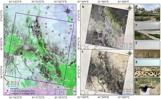
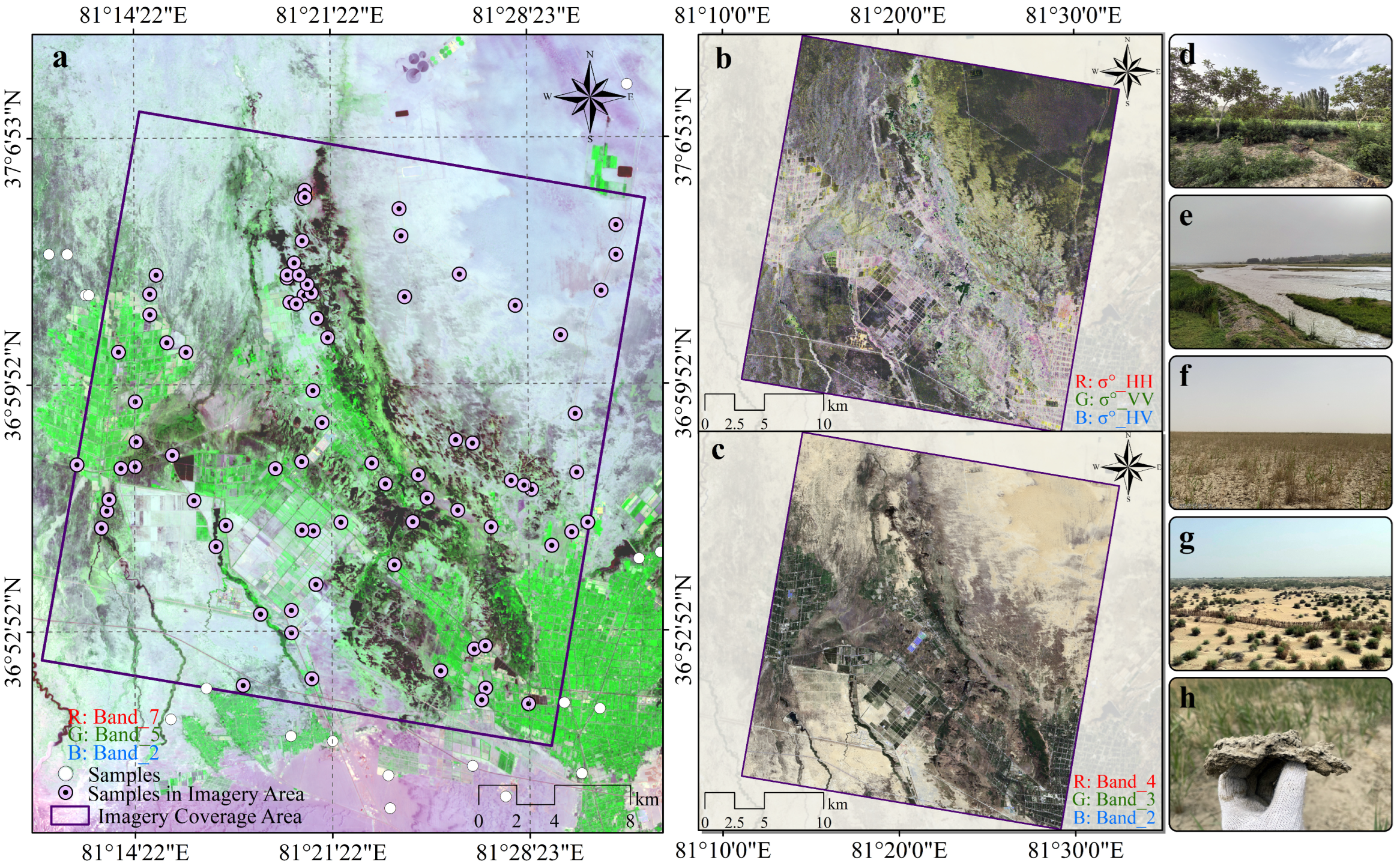
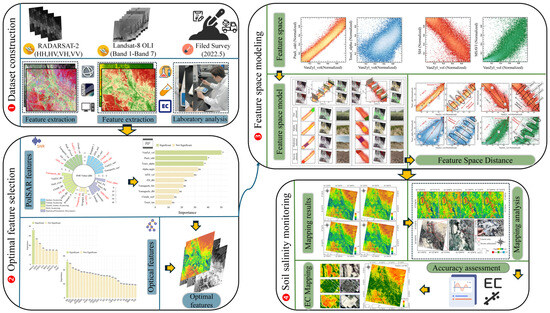
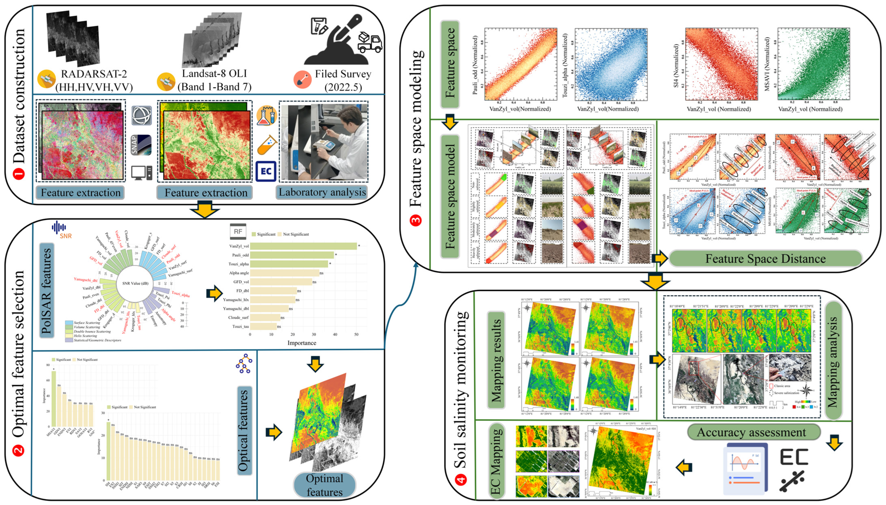
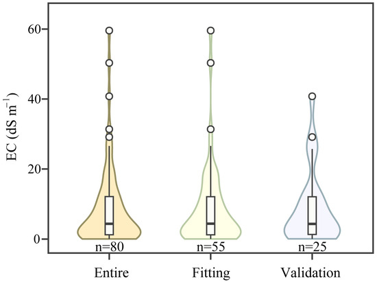
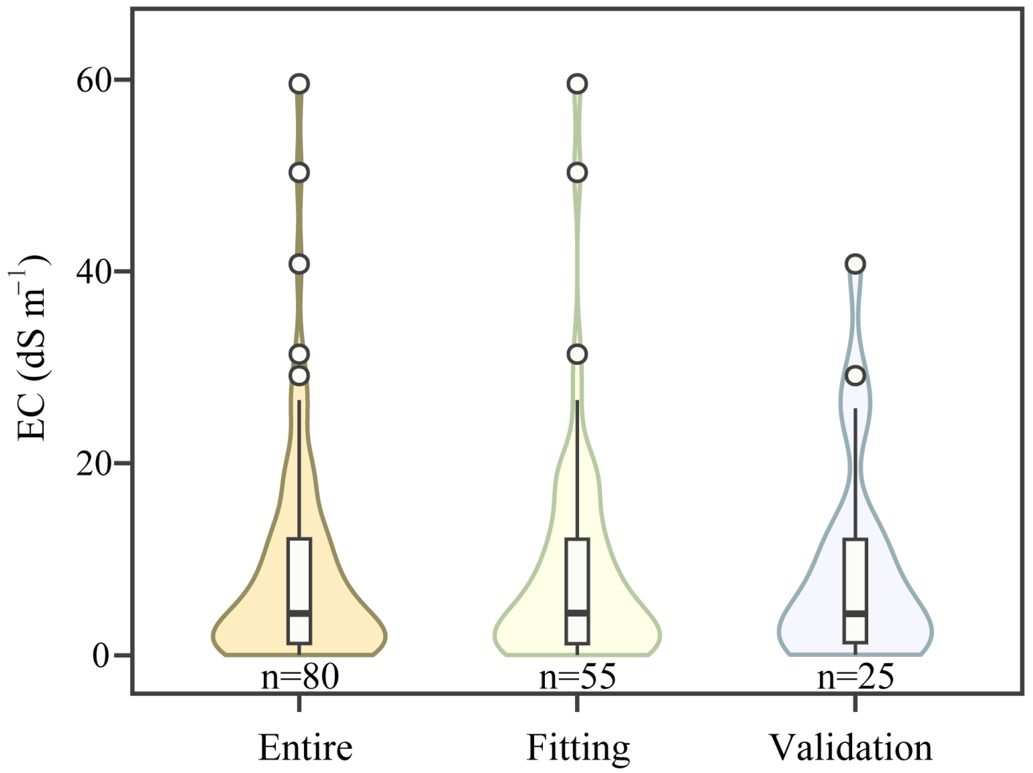
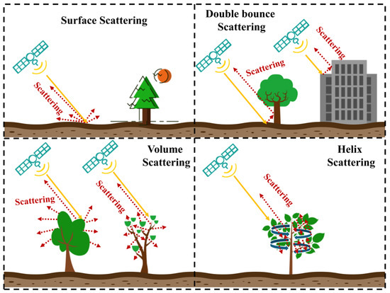
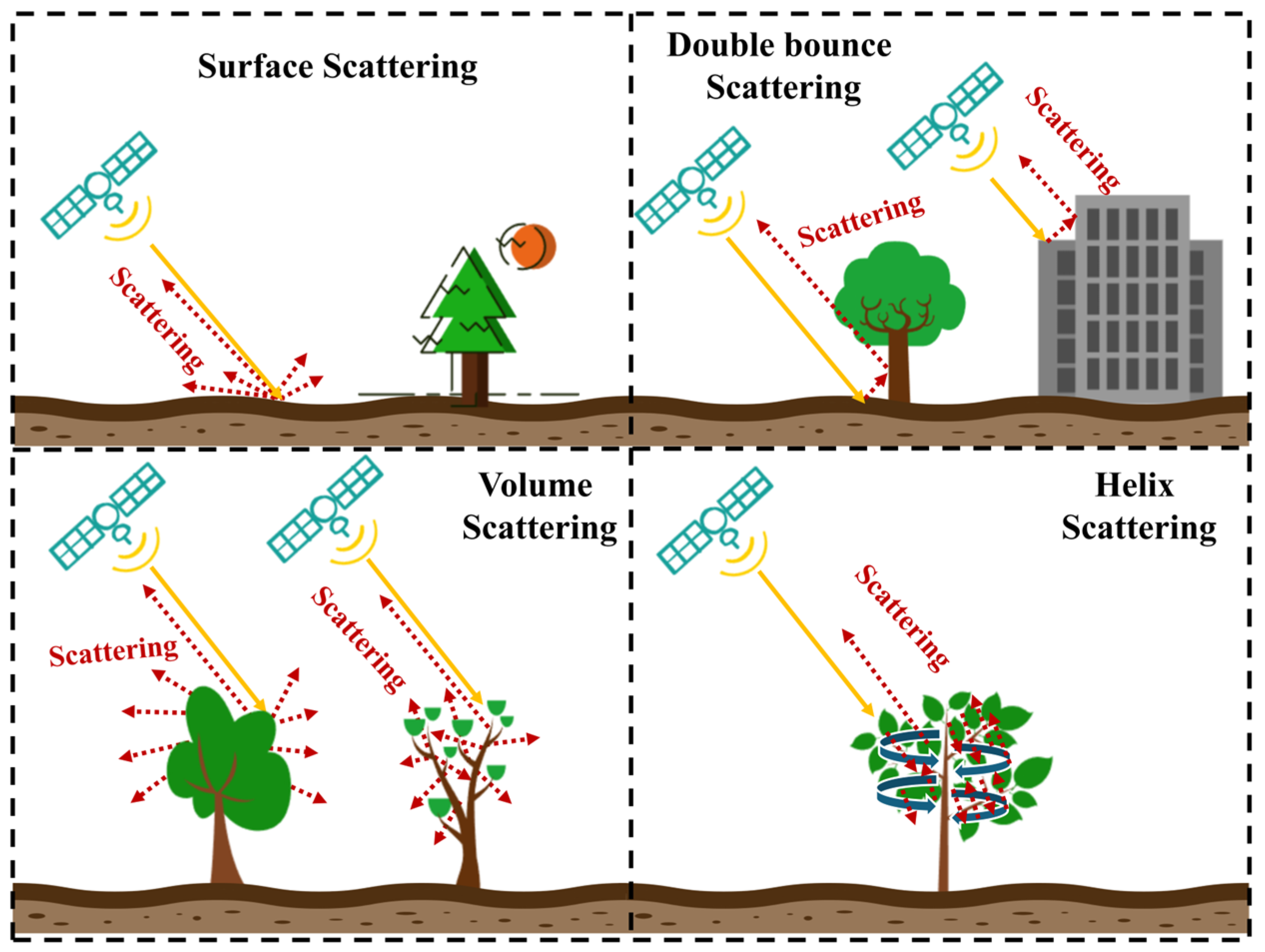
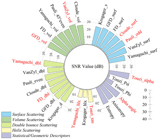
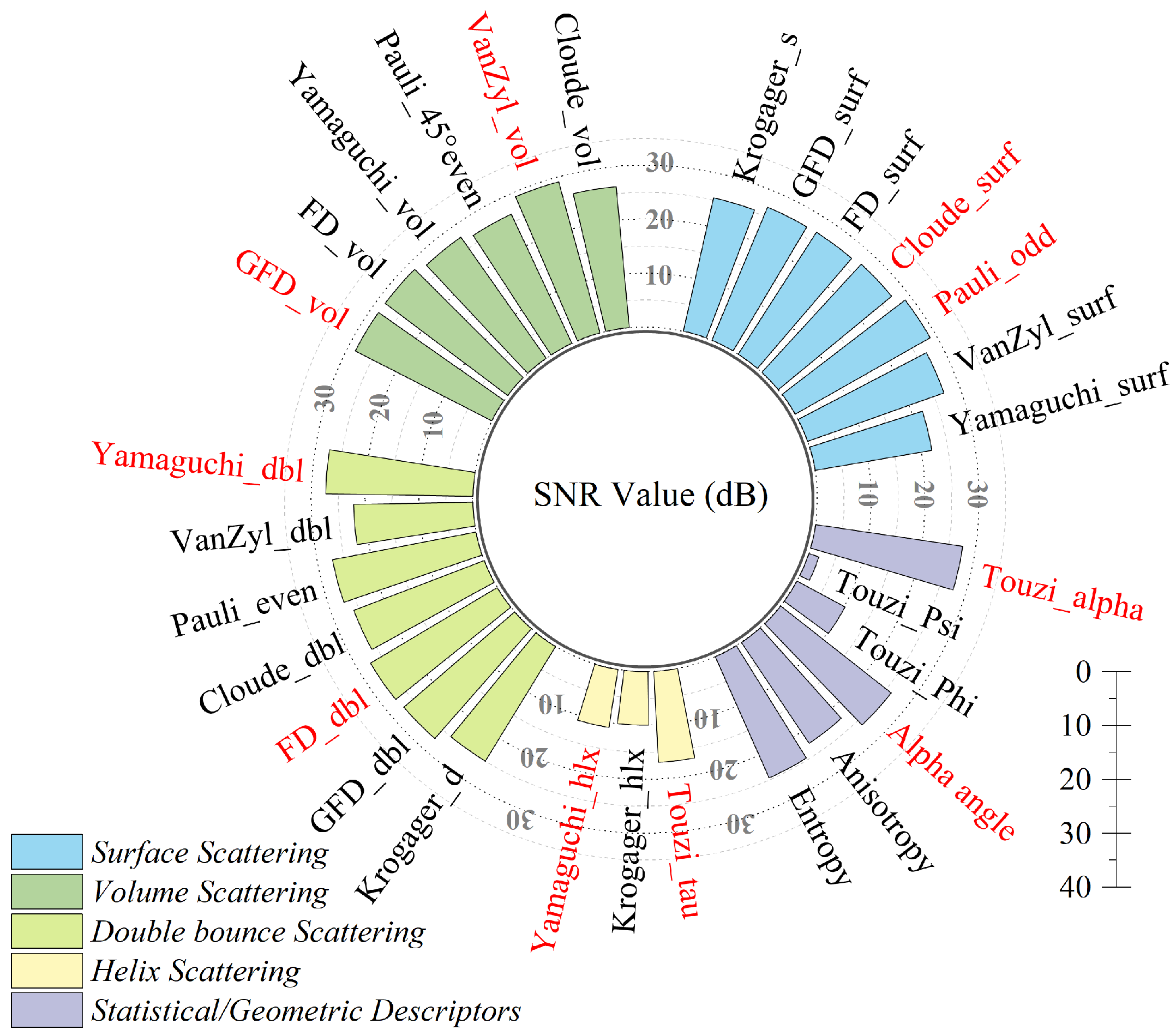
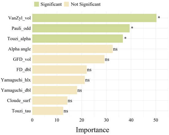
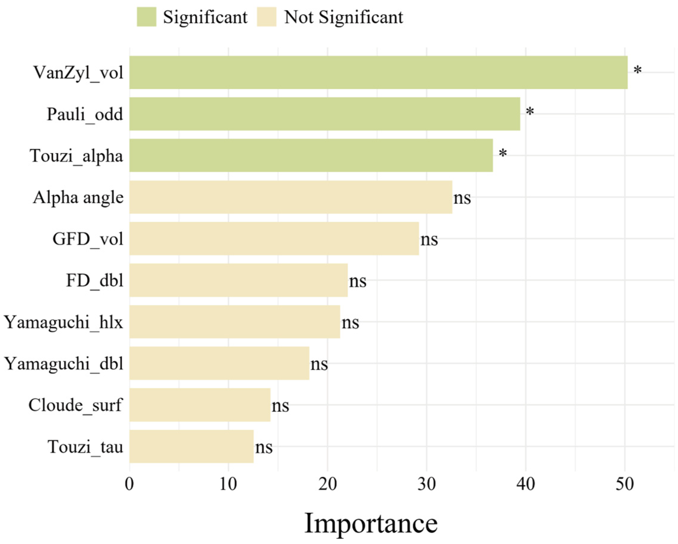
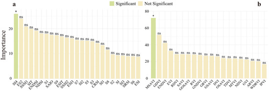
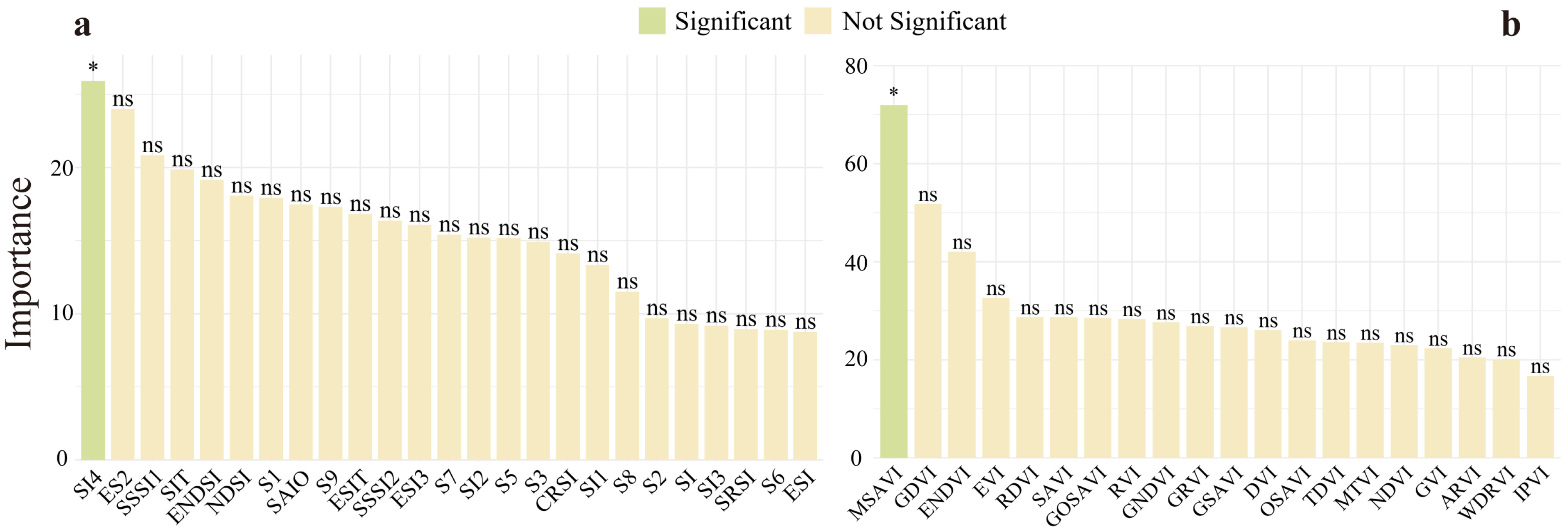
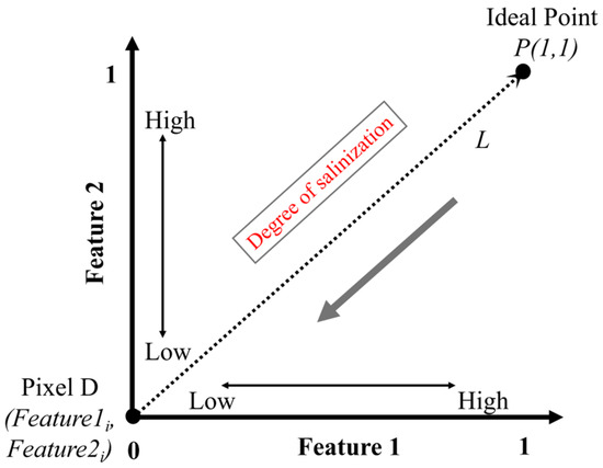
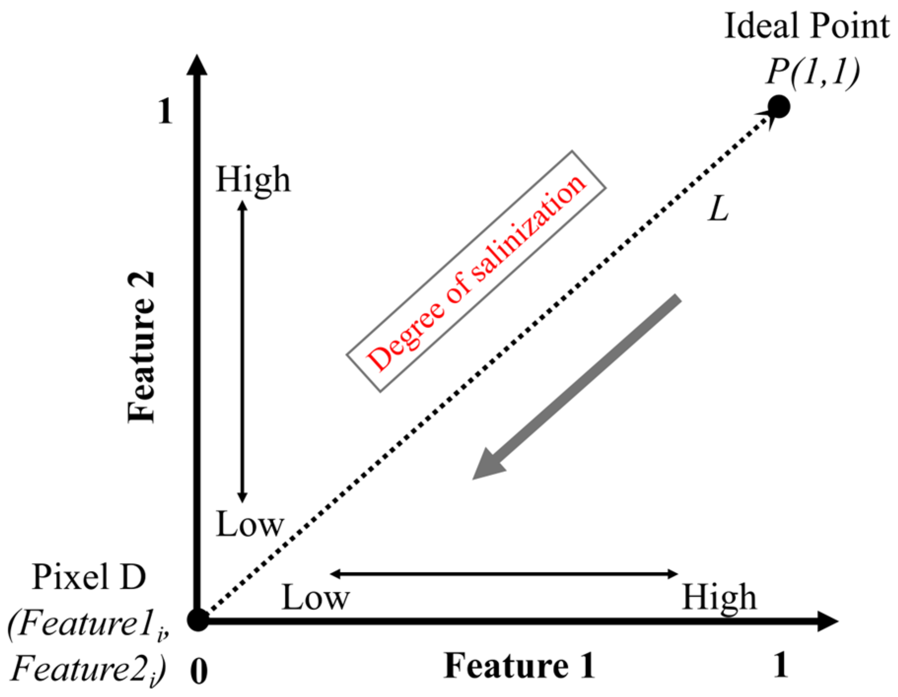
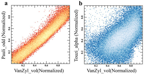
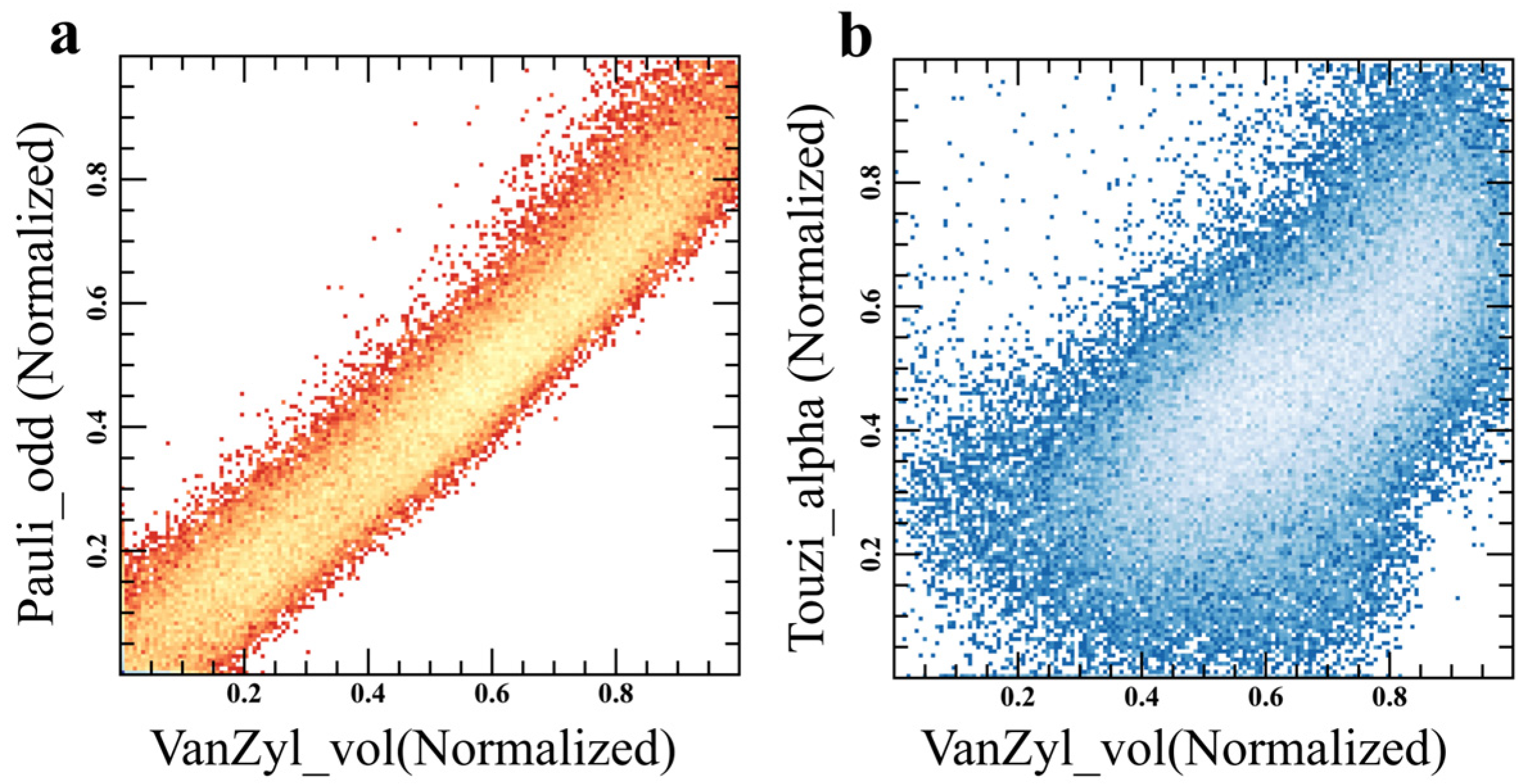
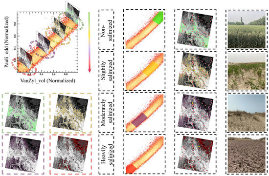
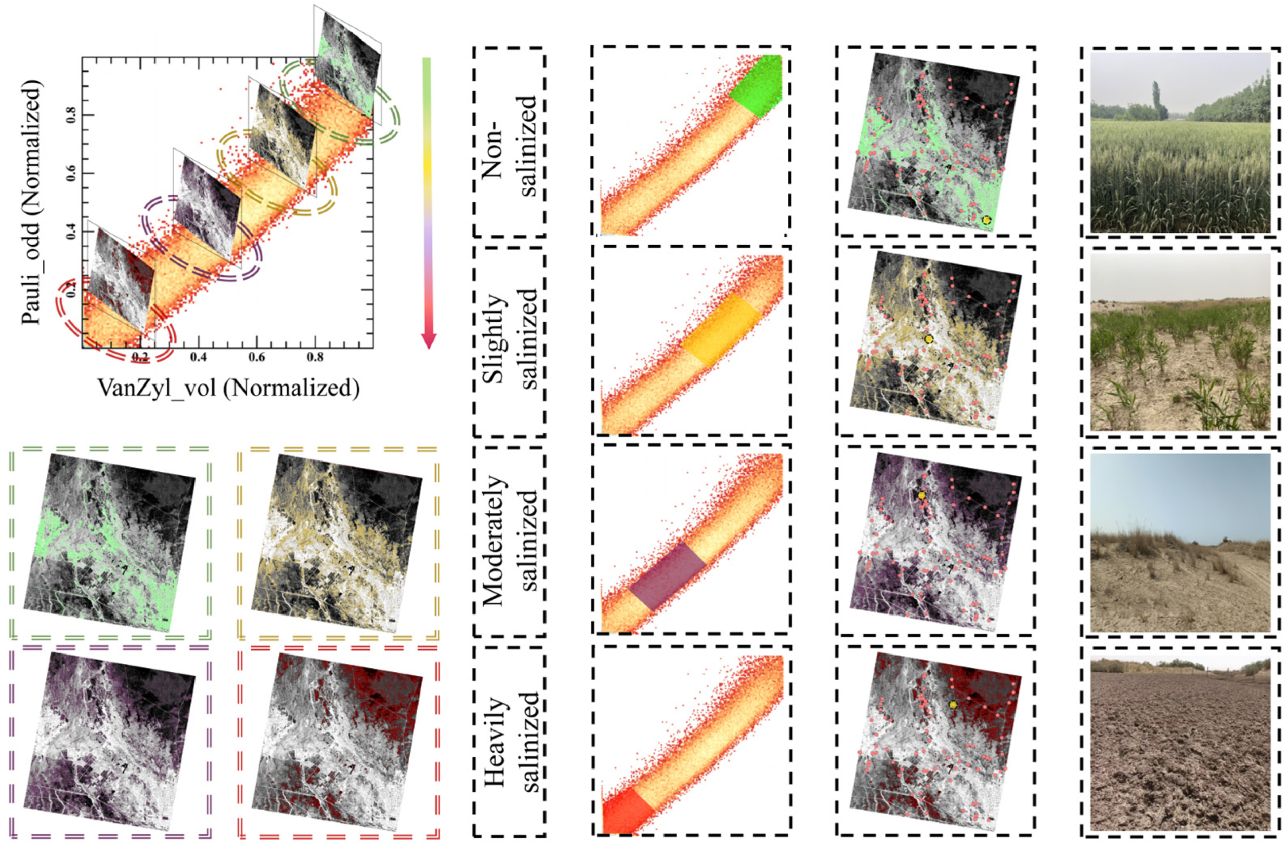
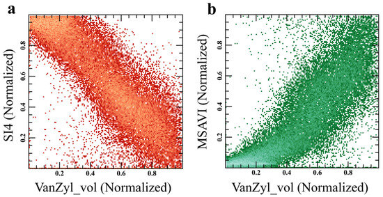
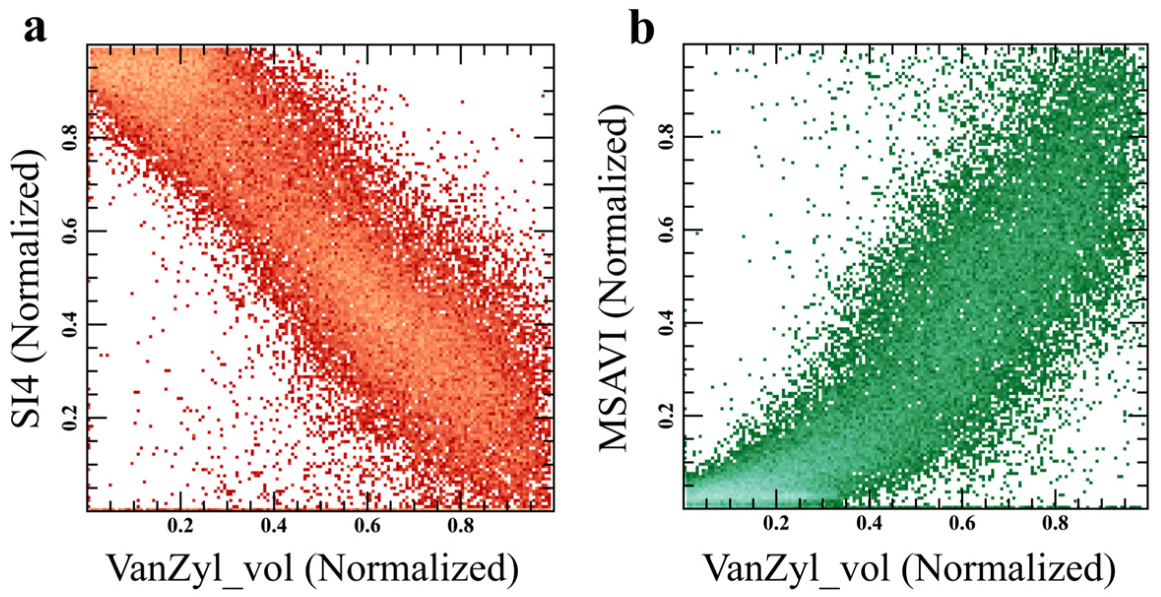
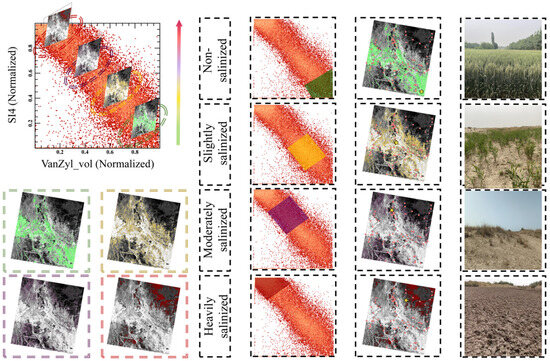
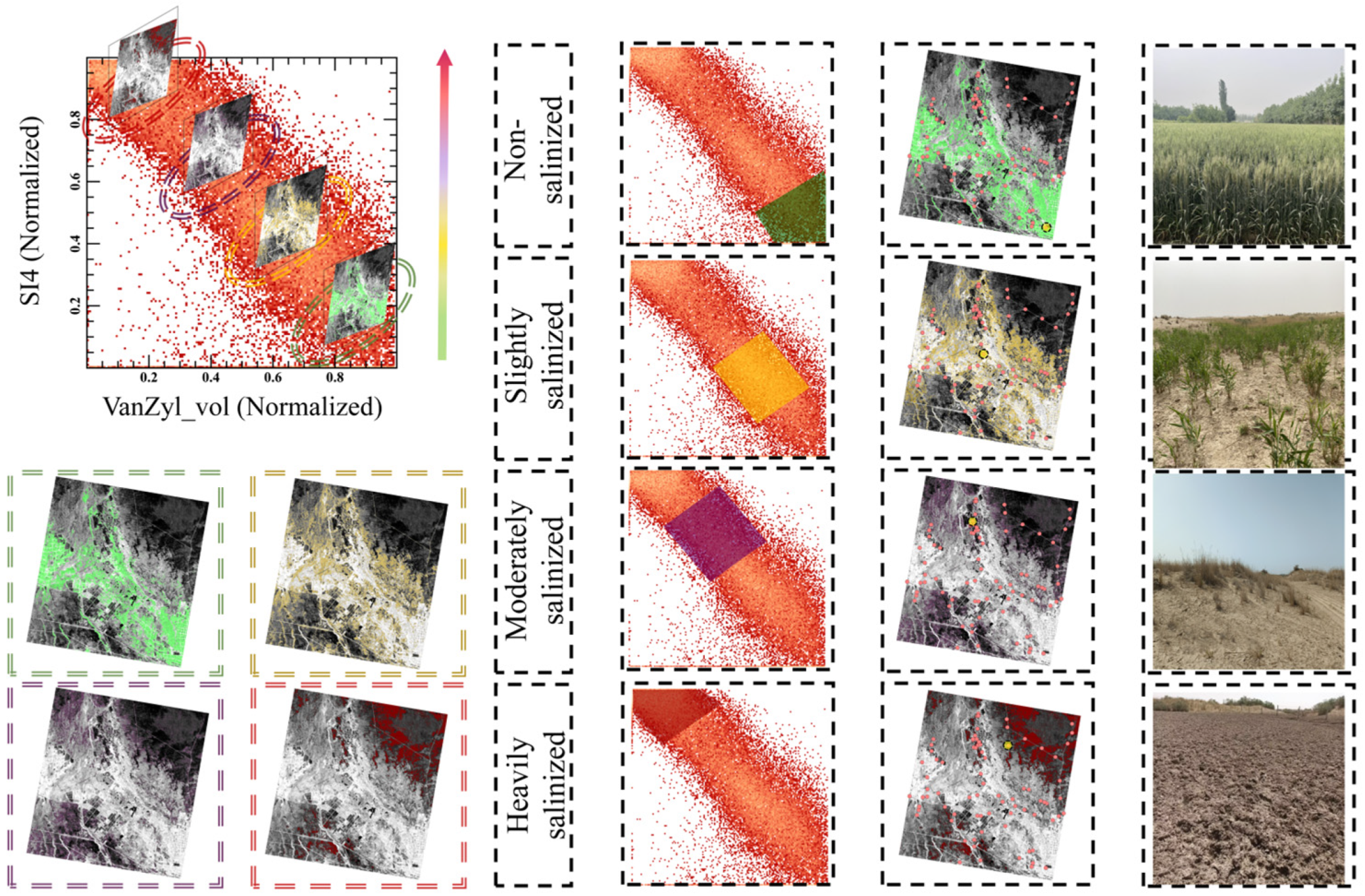
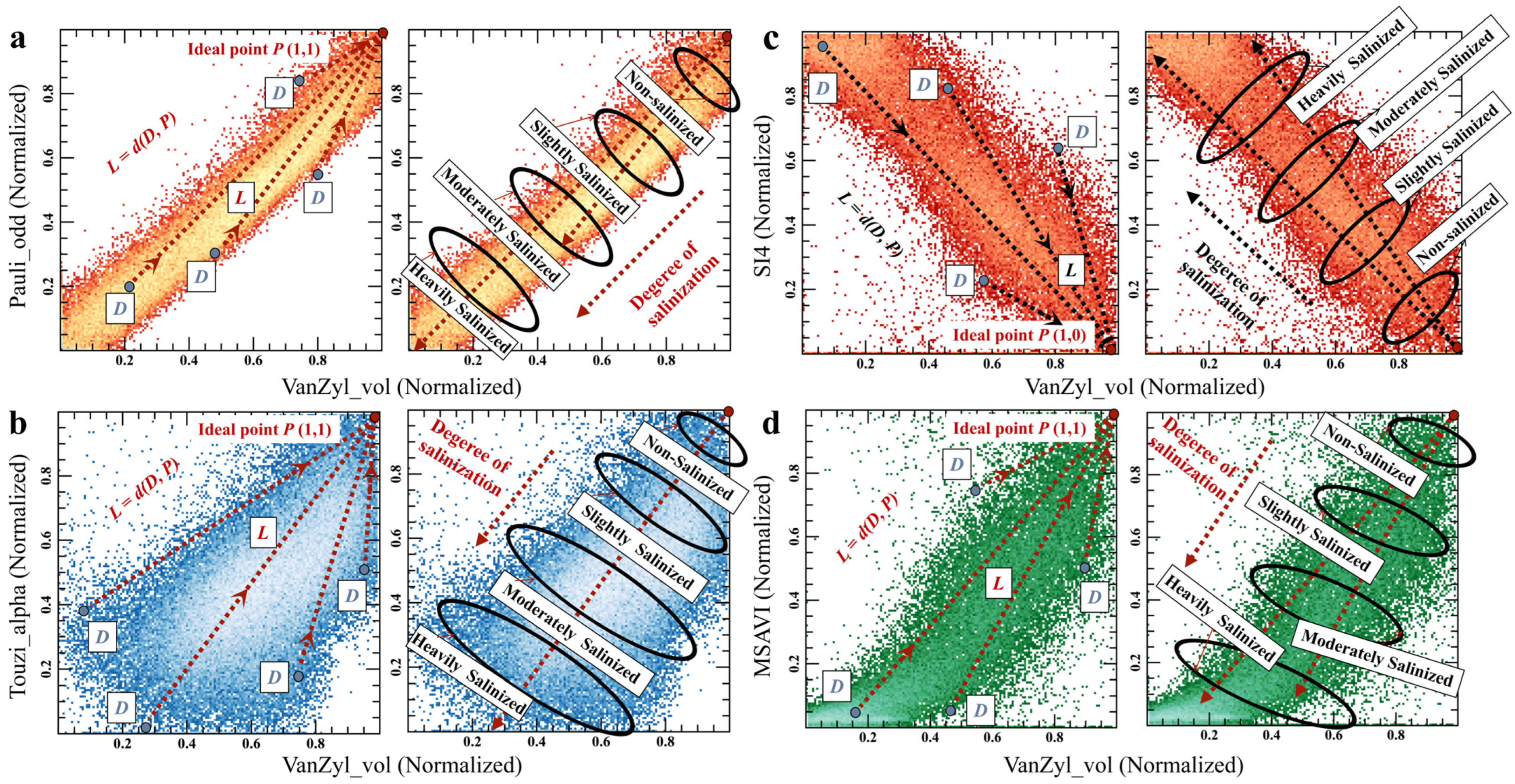
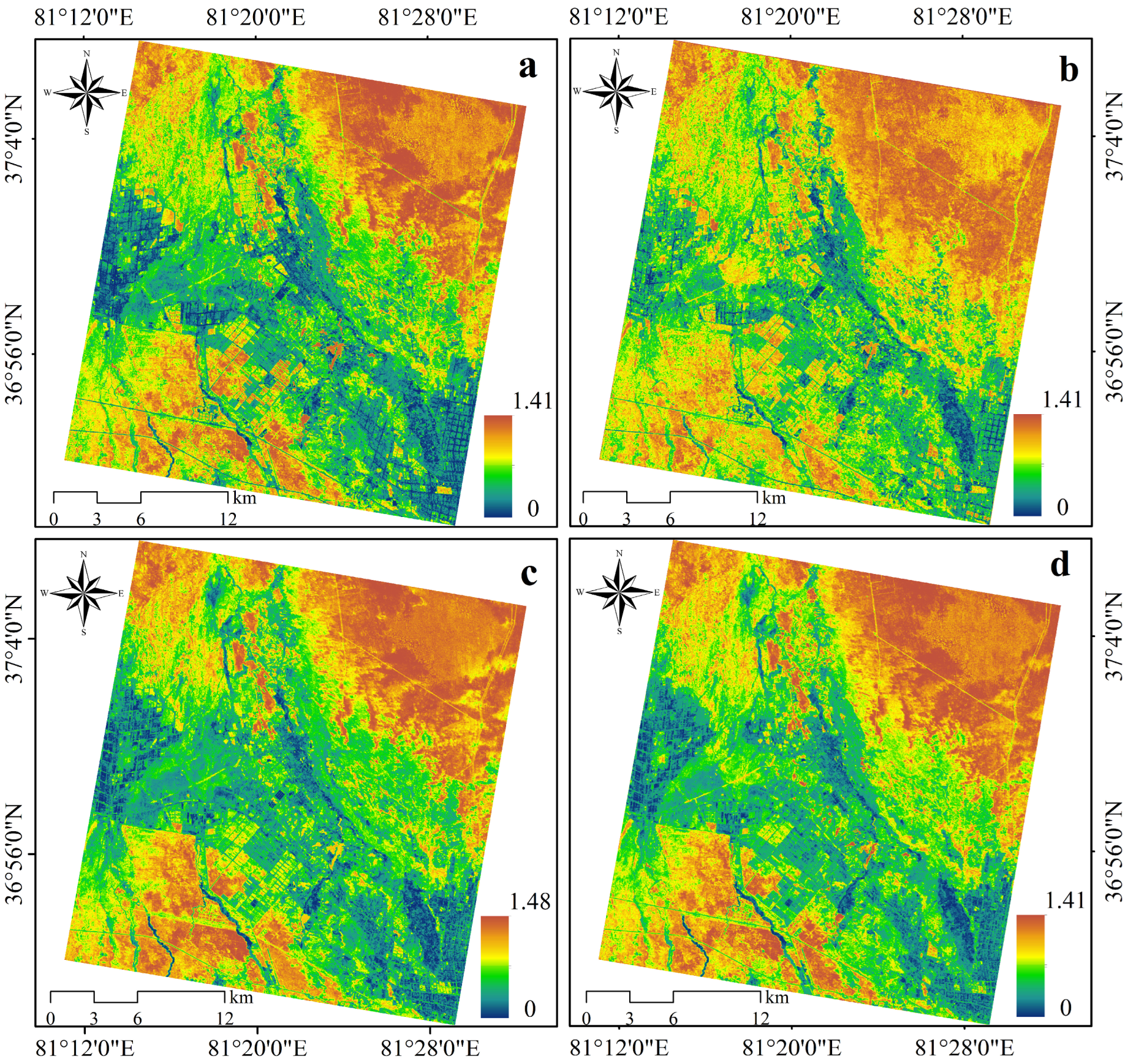
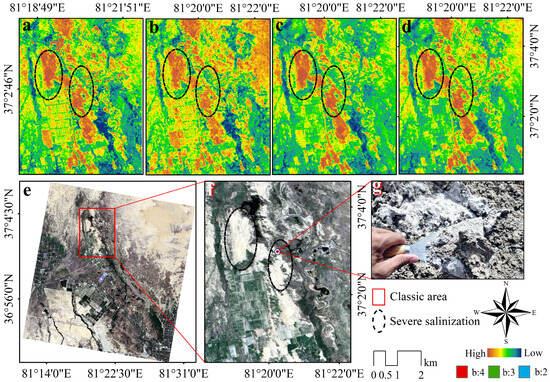
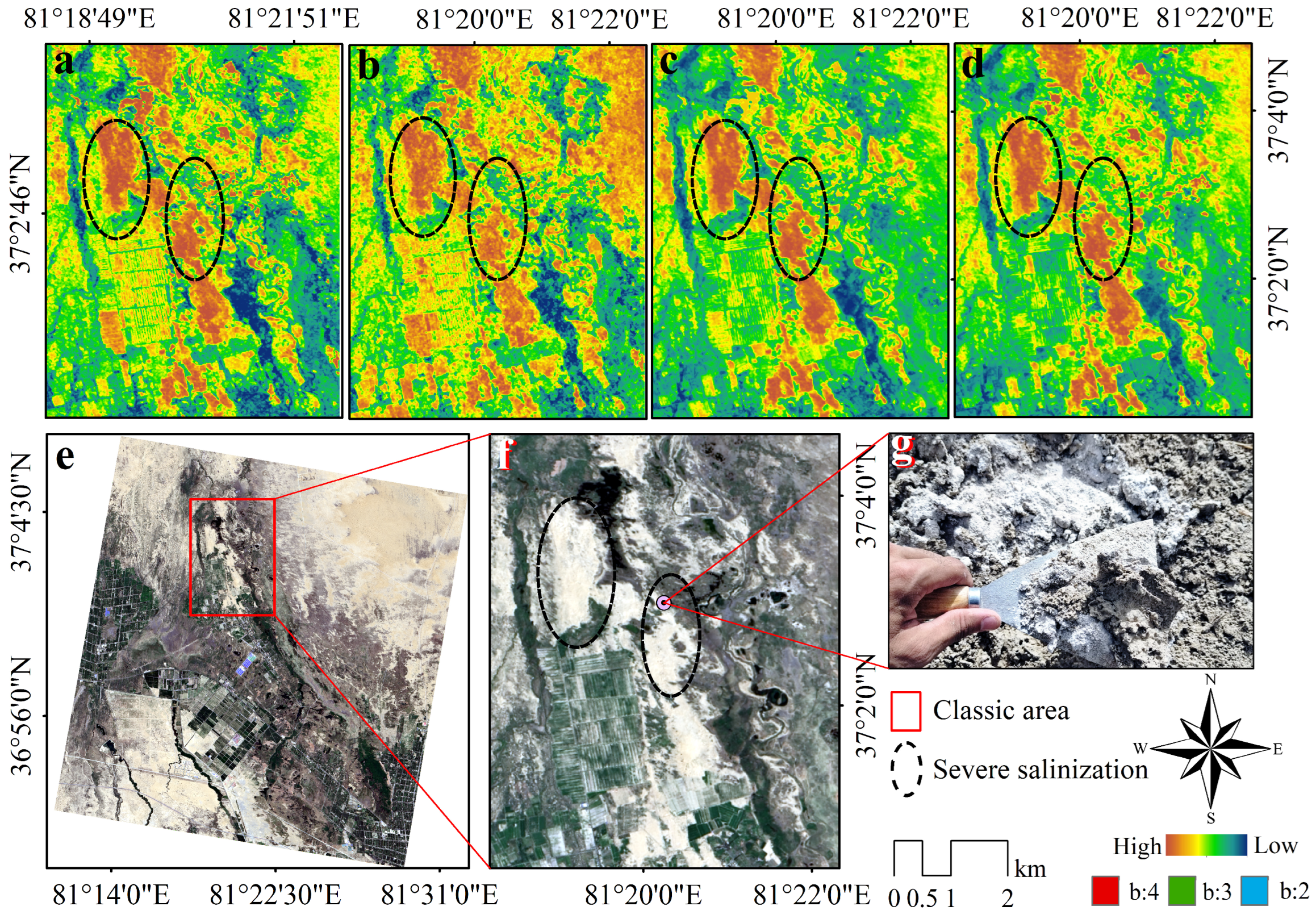
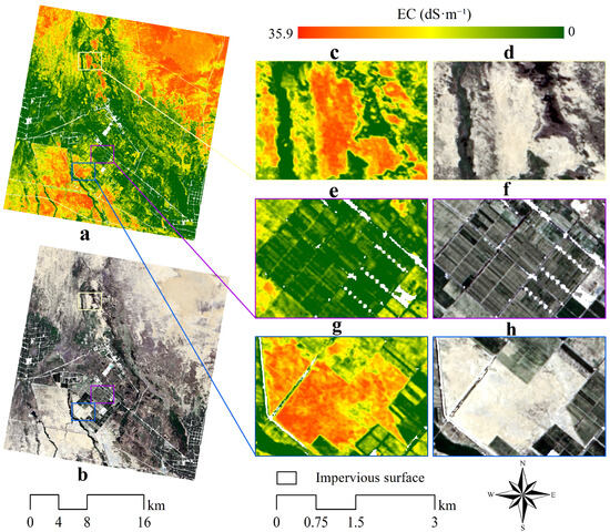
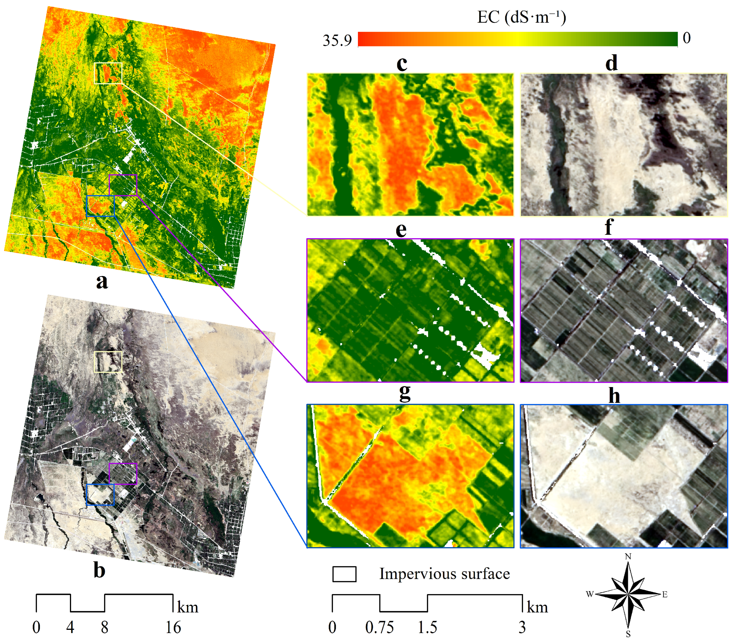

Disclaimer/Publisher’s Note: The statements, opinions and data contained in all publications are solely those of the individual author(s) and contributor(s) and not of MDPI and/or the editor(s). MDPI and/or the editor(s) disclaim responsibility for any injury to people or property resulting from any ideas, methods, instructions or products referred to in the content. |
© 2026 by the authors. Licensee MDPI, Basel, Switzerland. This article is an open access article distributed under the terms and conditions of the Creative Commons Attribution (CC BY) license.