


Highlights
What are the main findings?
- Terrain Ruggedness (TRI) and categorically encoded Land Cover act as the universally dominant error drivers across all global DEMs, with complex surface types systematically introducing positive elevation biases.
- Secondary to these shared factors, distinct sensor-specific mechanisms govern the remaining errors: Canopy Height for the X-band COP30, Topographic Position (TPI) for the C-band NASADEM, and absolute Elevation for the optical AW3D30.
What are the implications of the main findings?
- The results indicate that, in reprocessed datasets like NASADEM, radiometric factors (e.g., dense vegetation on ridges) and algorithmic processing (e.g., hydro-flattening in valleys) can overpower pure geometric smoothing effects.
- By successfully decomposing deterministic terrain biases from sensor-specific random noise (explaining ~40% of the total error variance), this study provides a physics-informed framework for developing more targeted elevation correction algorithms and improved regional DEM accuracy.
Abstract
Digital elevation models (DEMs) are foundational for critical tasks such as flood inundation simulation, disaster risk assessment, and ecosystem monitoring in coastal zones, yet their vertical accuracy is significantly compromised by complex terrain and surface characteristics. This study quantitatively decomposes the vertical errors of three 30 m global DEMs (COP30, NASADEM, and AW3D30) across the subtropical coastal region of Southeast China using ICESat-2 ATL08 data as a reference. By integrating an eXtreme Gradient Boosting (XGBoost) model with SHapley Additive exPlanations (SHAP), we successfully decoupled systematic biases from random noise. The results show that NASADEM achieved the lowest RMSE (7.775 m), followed by COP30 and AW3D30. While the Terrain Ruggedness Index (TRI) and categorically encoded Land Cover were identified as the universally dominant error drivers across all datasets, explainable analysis revealed distinct secondary mechanisms: X-band COP30 is notably susceptible to canopy height, exhibiting significant positive bias in forests exceeding 15 m; C-band NASADEM shows a systematic bias related to topographic position, typically overestimating ridges and underestimating valleys; and optical AW3D30 is significantly affected by stereo-matching errors. Furthermore, the analysis quantified a systematic error component of ~40%. These findings provide a data-driven basis for DEM selection and highlight that accuracy improvements should prioritize vegetation removal for radar DEMs and enhanced stereo-matching for optical models.
1. Introduction
Digital elevation models (DEMs) are foundational geospatial datasets that quantitatively represent Earth’s surface topography. They serve as primary inputs for deriving critical terrain attributes such as slope, aspect, curvature, flow accumulation, and topographic wetness index, which underpin a broad spectrum of Earth-system applications, including hydrological modeling, InSAR monitoring, flood inundation simulation, landslide susceptibility assessment, soil erosion prediction, ecosystem service evaluation, and climate change impact studies in coastal zones [1,2,3,4,5]. In low-lying coastal and subtropical regions, where even minor vertical inaccuracies can translate into substantial uncertainties in modeled inundation extent and hazard exposure, the reliability of DEMs is particularly critical [6,7].
Although freely available global DEMs such as SRTM, NASADEM, AW3D30, Copernicus DEM, and more recent products (e.g., FABDEM) provide near-global coverage, they exhibit systematic and random vertical errors that vary strongly with terrain complexity, land-cover type, sensor characteristics, and acquisition conditions [8]. Reported biases have been linked to vegetation canopy penetration limitations, stereo-matching failures on steep or low-texture surfaces, aspect-dependent illumination and geolocation offsets, and temporal mismatches between DEM acquisition and reference data [5,9,10,11,12]. Global-scale assessments typically report overall RMSE values of 6–10 m for 30 m DEMs [5,9], yet they often fail to resolve the specific error mechanisms operating in subtropical coastal zones characterized by rugged terrain and dense vegetation cover—environments that combine steep slopes, closed-canopy forests/mangroves, and frequent cloud cover [4,6]. Moreover, there is no clear consensus regarding the dominant driver of vertical error: some studies identify land cover (particularly forests) as the primary factor [6,9], while others emphasize terrain slope [5,10,13].
In the present study, we address this gap by applying an eXtreme Gradient Boosting (XGBoost) model combined with SHapley Additive exPlanations (SHAP) to quantitatively decompose vertical errors in selected global DEMs across a subtropical coastal study area with rugged terrain and dense vegetation. XGBoost captures complex nonlinear relationships and feature interactions, while SHAP delivers consistent, model-agnostic interpretability by attributing each prediction to individual drivers based on cooperative game theory [14]. This XGBoost–SHAP framework has demonstrated high predictive accuracy and explanatory power in remote-sensing applications, including landslide susceptibility mapping [15], ecosystem-service trade-off analysis [16], urban flood-risk assessment [17], and compound wind droughts and heat waves driving mechanism analysis [18]. By adopting this approach, the current work provides a transparent, data-driven ranking of error sources that can guide both DEM selection and insights for developing targeted bias-correction strategies in data-scarce subtropical coastal environments. Crucially, the main scientific contribution of this study extends fundamentally beyond a regional accuracy assessment. Unlike conventional evaluations that primarily focus on quantifying overall error magnitudes, this study advances the methodology by mathematically decoupling correctable deterministic biases (driven by explicitly quantified geodetic and cartographic factors) from irreducible stochastic sensor noise. Through this physics-informed decoupling, we establish a globally transferable framework capable of operationally upgrading legacy DEMs in highly dynamic coastal environments.
2. Study Area and Datasets
2.1. Study Area
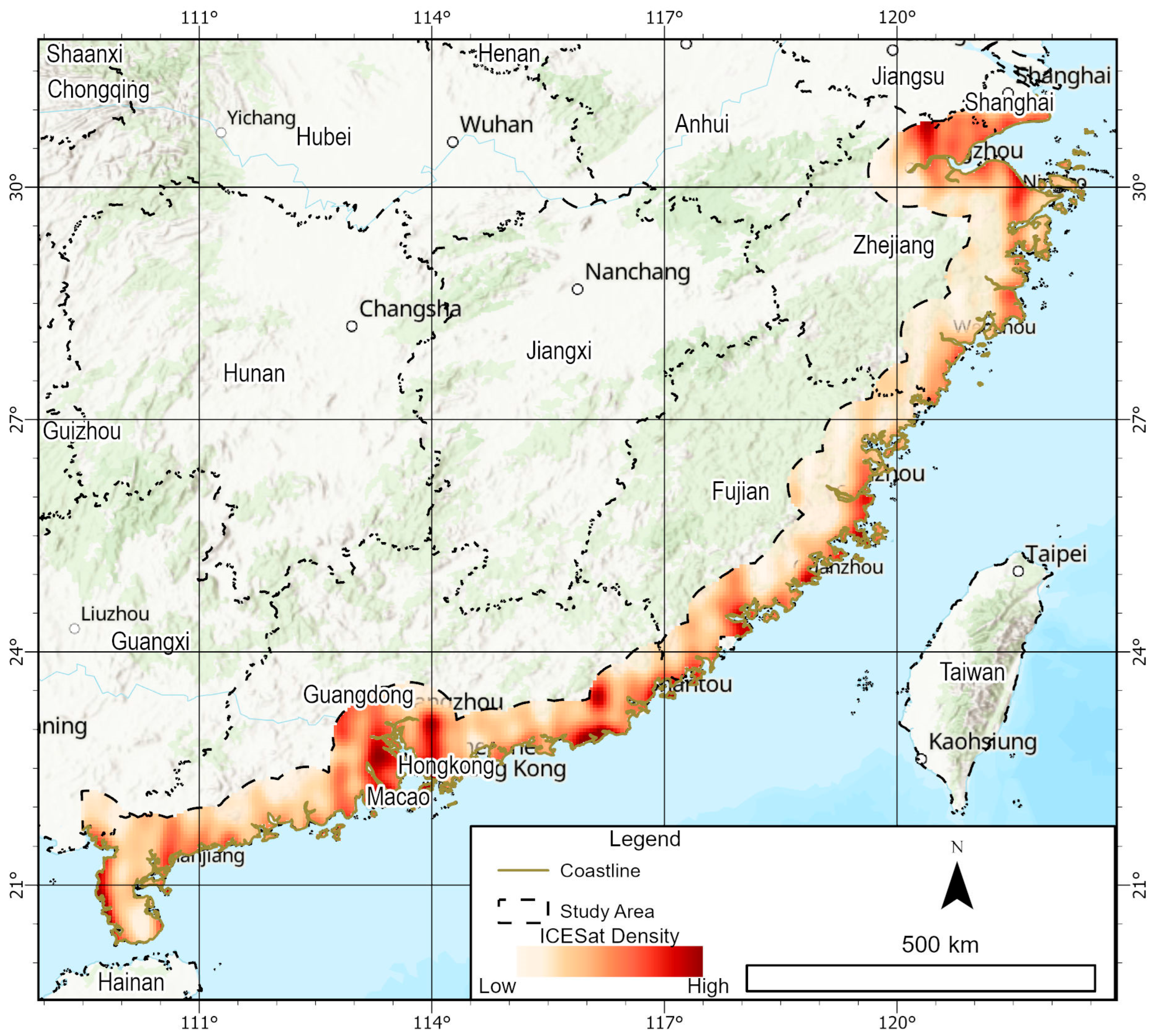
This research focuses on the Southeast China coastal region (20°N–31°N, 109.5°E–122.5°E), defined as a 50 km buffer extending inland from the coastline (Figure 1). The coastline reference was derived from the Natural Earth 10m physical vector dataset (ne_10m_coastline). Consequently, the study covers a total area of approximately 197,235 km2, spanning the provinces of Zhejiang, Fujian, and Guangdong. This region represents one of China’s most economically dynamic and anthropogenically active zones [19]. The topography is complex, ranging from sea level to a peak of ~1500 m, with land cover transitioning from dense urban agglomerations to subtropical forests. Specifically, this region poses uniquely compounded challenges for global DEM generation compared to flatter or arid areas. First, the rapid geomorphological transition from coastal plains to rugged hills induces severe geometric distortions, such as foreshortening, layover, and radar shadow in SAR-based DEMs (NASADEM, COP30), while simultaneously causing extensive occlusion and matching failures in optical stereo-pairs (AW3D30). Second, the ubiquitous coverage of dense, closed-canopy subtropical broadleaf forests severely restricts signal penetration. The short-wavelength X-band (COP30) and optical sensors (AW3D30) are almost entirely intercepted by the canopy top, while even the C-band (NASADEM) suffers from significant volume scattering, introducing a systematic positive elevation bias. Finally, the frequent cloud cover and high atmospheric moisture inherent to this monsoon coastal climate further degrade the availability of clear optical imagery and introduce tropospheric phase delays in InSAR processing. These characteristics provide a robust setting for evaluating the spatial accuracy of global DEMs in heterogeneous coastal environments.
Figure 1.
Topography of the study area (Southeast China coast) showing the spatial density distribution of ICESat-2 validation points.
2.2. DEMs
In this study, three open access global DEMs with a pixel spacing of approximately 30 m (1 arc-second) were evaluated: the ALOS World 3D-30 m (AW3D30), the NASADEM, and the Copernicus DEM (COP30). All datasets were acquired from the OpenTopography platform (https://opentopography.org, accessed on 9 January 2026). It is critical to clarify that this 30 m metric refers strictly to the gridded pixel spacing rather than the true spatial resolution of these DEMs. As highlighted by [20], grid spacing cannot be assumed to equal the true spatial resolution, which is often significantly coarser due to sensor footprint limitations and oversampling during the DEM generation process.
The AW3D30 is a global optical Digital Surface Model (DSM) generated from stereoscopic imagery acquired by the Panchromatic Remote-sensing Instrument for Stereo Mapping (PRISM) onboard the Advanced Land Observing Satellite (ALOS) between January 2006 and April 2011 [21]. Unlike the active InSAR techniques used for NASADEM and COP30, AW3D30 relies entirely on passive optical stereophotogrammetry. Consequently, its acquisition is fundamentally constrained by cloud occlusion and requires high visual surface contrast to successfully perform stereo-matching. Cartographically, areas with homogeneous textures (e.g., coastal waters, mudflats) often suffer from correlation failures, leading to localized interpolation artifacts. The dataset is distributed in 1° × 1° tiles. It adopts the WGS84 ellipsoid as the horizontal reference and the EGM96 geoid as the vertical datum.
NASADEM is a void-free, near-global elevation model produced by reprocessing the original Shuttle Radar Topography Mission (SRTM) data. The core measurement is derived from C-band (wavelength ~5.6 cm) Synthetic Aperture Radar (SAR) interferometry. From an acquisition perspective, the C-band signal partially penetrates vegetation canopies, capturing a phase center situated between the canopy top and bare earth. This wavelength characteristic is critical for understanding signal penetration in vegetated environments compared to shorter-wavelength sensors. Cartographically, the NASADEM reprocessing workflow applied aggressive void-filling and hydro-flattening algorithms. While these procedures enforced hydrological connectivity, they inherently acted as low-pass filters, modifying the raw geodetic elevations in deep valleys and coastal wetlands. Furthermore, the reprocessing workflow incorporated auxiliary data, including ICESat/GLAS elevations and ASTER GDEM3 data, to aid in phase unwrapping and void filling [22]. This wavelength characteristic is critical for understanding signal penetration in vegetated canopies compared to shorter-wavelength sensors. NASADEM products are provided in 1° × 1° tiles with a resolution of 1 arc-second, referenced horizontally to WGS84 and vertically to the EGM96 geoid.
The Copernicus DEM (COP30) is a 1-arc-second DSM derived from the WorldDEM, which is based on radar satellite data acquired during the TanDEM-X mission (December 2010 to January 2015). The primary objective of the mission was to generate a consistent, high-precision global DSM using X-band (wavelength ~3.1 cm) SAR interferometry. Geodetically, it benefits from a highly stable baseline calibration. However, regarding its acquisition characteristics, the much shorter X-band wavelength has virtually zero penetration capability through dense subtropical foliage, meaning its raw measurements are highly sensitive to the uppermost canopy structure. The product is provided in geographic coordinates referenced to the WGS84 horizontal datum. Notably, unlike AW3D30 and NASADEM, the vertical reference of COP30 is the EGM2008 geoid, necessitating datum unification prior to accuracy assessment [9].
2.3. ICESat-2 ATL08
The Advanced Topographic Laser Altimeter System (ATLAS) onboard NASA’s ICESat-2 satellite (launched in 2018) provides the altimetric reference for this study, which is from the National Snow and Ice Data Center (https://nsidc.org/data/icesat/data, accessed on 9 January 2026). ATLAS utilizes photon-counting LiDAR technology to acquire dense surface elevation profiles along six beams [23]. We employed the Level-3A Land and Vegetation Height product (ATL08, Version 006), specifically extracting the slope-corrected terrain height (h_te_best_fit) to represent the ground surface. To mitigate atmospheric scattering and solar background noise, the analysis was strictly restricted to the high-energy strong beams [24]. The dataset, covering the period from January 2021 to December 2022, was accessed via the National Snow and Ice Data Center (NSIDC). Notably, the ATL08 product is referenced to the WGS84 ellipsoid. To ensure vertical datum consistency during validation, we retained the native ICESat-2 ellipsoidal heights and conversely transformed the orthometric heights of all target global DEMs (referenced to EGM96/EGM2008) into the WGS84 ellipsoidal system prior to the error calculation.
2.4. Covariates for Error Modeling
To systematically quantify the error mechanisms inherent to different imaging modalities, we constructed a feature space comprising nine covariates that characterize the geometric, ecological, and spatial context of each validation point (Table 1).
Table 1.
Summary of covariates used for vertical error modeling.
The geometric variables, which serve as the primary drivers of distortions in both SAR and optical stereo-matching [25,26], include the Terrain Ruggedness Index (TRI), Topographic Position Index (TPI), Slope, Aspect, and Reference Elevation. To ensure a consistent morphological reference across all global DEM evaluations, all derivative topographic indices (Slope, Aspect, TRI, TPI) were uniformly computed from the void-free NASADEM. Specifically, TRI was calculated following the methodology of [27] using a 3 × 3 window to quantify local surface roughness and potential signal decoherence. TPI was derived based on [28] to measure the relative elevational position of a pixel, effectively distinguishing between convex ridges and concave valleys, which is critical for analyzing radar shadow and water vapor stratification effects [29,30]. The calculation of these spatial neighborhood-based indices (TRI and TPI) inherently aggregates regional topographic context, which helps to physically accommodate the coarser true spatial resolution of reprocessed DEMs. Crucially, to mitigate the endogeneity bias that would arise from using the target DEMs themselves as explanatory variables, the high-precision ICESat-2 elevation was employed as the independent reference for absolute terrain height.
Ecological variables were integrated to account for vegetation scattering and surface heterogeneity. We utilized the global canopy height map generated by [31], a probabilistic deep learning model that fuses GEDI LiDAR data with Sentinel-2 imagery, to represent vertical vegetation structure. This variable is essential for decoupling the penetration depth of radar signals from the canopy-top bias in optical models. Additionally, the Normalized Difference Vegetation Index (NDVI) was derived from Landsat-8 imagery acquired during the study period as a proxy for vegetation density and health. To capture the influence of diverse surface materials, the ESA WorldCover v200 dataset (10 m) was used to categorize Land Use/Land Cover (LULC) conditions [32], which captures the full diversity of surface types present in our coastal study area, specifically encoded as Class 10: Trees, Class 20: Shrubland, Class 30: Grassland, Class 40: Cropland, Class 50: Built-up, Class 60: Bare/sparse vegetation, Class 80: Water bodies, Class 90: Herbaceous wetland, and Class 95: Mangroves.
Finally, to address coastal-specific atmospheric and topographic effects, we incorporated a spatial variable, Distance to Coast, calculated as the Euclidean distance from each validation point to the nearest coastline. This factor serves as a proxy for the gradients of atmospheric water vapor and complex dielectric properties in littoral zones [33,34]. Prior to modeling, all raster covariates were spatially harmonized. Continuous variables were resampled using cubic convolution, while categorical variables used nearest neighbor interpolation, ensuring all layers were aligned to a unified 30 m grid consistent with the target global DEMs. The covariate values were then extracted to the corresponding ICESat-2 footprint locations for input into the XGBoost model. Following this extraction, a preliminary Pearson correlation analysis of all continuous covariates was conducted to diagnose potential multicollinearity (Figure S1 in the Supplementary Materials). Because an extreme correlation (r = 0.98) was observed between the TRI and Slope, Slope was explicitly excluded from the final modeling dataset to ensure the stability of subsequent SHAP value allocations.
3. Methods
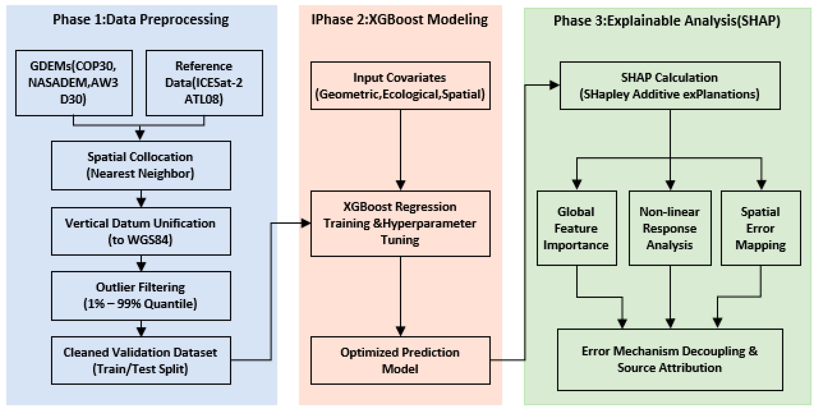
The methodological framework of this study is illustrated in Figure 2 and comprises three primary stages. First, we prepare the dataset by extracting reliable RCPs from ICESat-2 ATL08. Second, we implement XGBoost modeling to learn the error patterns. Third, we perform an explainable analysis using SHAP values and generate the final spatial error map for the study area.
Figure 2.
Workflow of the explainable error analysis framework, integrating XGBoost modeling and SHAP interpretation.
3.1. Data Preprocessing
Following the data selection criteria described in Section 2.3, the preprocessing workflow consisted of three steps: spatial collocation, vertical datum unification, and outlier filtering.
(1) For each ICESat-2 footprint retained from the strong-beam filtering, the corresponding elevation value from each global DEM was extracted. A nearest-neighbor sampling approach was employed to align the RCP coordinates with the center of the nearest global DEM pixel, avoiding interpolation artifacts.
(2) To ensure consistency between the datasets, the vertical reference systems were harmonized. The ICESat-2 ATL08 product provides heights referenced to the WGS84 ellipsoid (h), whereas the global DEMs provide orthometric heights (H) referenced to Earth Gravitational Models. The geoid undulation (N) at each RCP location was calculated using the EGM2008 model for COP30 and the EGM96 model for NASADEM and AW3D30. The orthometric heights of the global DEMs were then converted to ellipsoidal heights using the relationship
where h denotes the converted ellipsoidal height, and H is the original orthometric height.
h = H + N
(3) Outlier Filtering Residual anomalies (e.g., due to cloud contamination or processing artifacts) may persist in the dataset despite initial quality flagging. To mitigate their impact on the global error metrics, elevation differences (dh = hDEM − hICESat-2) were calculated. Data points falling outside the 1% and 99% quantiles of the error distribution were identified as outliers and excluded from the subsequent analysis [35].
3.2. XGBoost Modeling
To reconstruct the complex non-linear relationship between elevation errors and the driving covariates, we employed the Extreme Gradient Boosting (XGBoost) regression algorithm. XGBoost is a scalable implementation of the gradient boosting framework that constructs an ensemble of K regression trees (fk) in a sequential manner. The predicted error for an instance is obtained by summing the outputs of these additive functions:
where represents the space of regression trees. At each iteration t, the algorithm minimizes a regularized objective function :
In this study, the squared error loss , was adopted to penalize large residuals. The regularization term controls model complexity based on the number of leaves T and leaf weights w, thereby preventing overfitting [17].
Prior to model training, the dataset underwent the outlier filtering described in Section 3.1 and was randomly partitioned into a training set (80%) and an independent testing set (20%). To identify the optimal hyperparameter configuration, we implemented a Randomized Search (RandomizedSearchCV) strategy coupled with 3-fold cross-validation. The optimization process aimed to minimize the Root Mean Square Error (RMSE). The search space included: number of estimator [300, 1000], maximum depth [6, 15] to capture deep interaction effects, learning rate [0.01, 0.1], and regularization parameters (min_child_weight and subsample ratios). The final predictive performance of the XGBoost model was evaluated on the held-out testing set using the Coefficient of Determination (R2). Furthermore, to ensure the mathematical and physical validity of the categorical LULC variable (ESA WorldCover), we utilized XGBoost’s native categorical data support rather than treating the nominal class codes (e.g., 10, 20, 50) as continuous integers. This advanced feature optimally partitions categorical levels based on their nominal categories without imposing any artificial ordinal relationship. Crucially, compared to traditional one-hot encoding, this native support preserves LULC as a single, unified feature, thereby preventing the fragmentation of SHAP importance scores and allowing for a coherent physical interpretation of land surface types.
To justify the selection of XGBoost, we conducted a preliminary comparison with the Random Forest (RF) algorithm. The results showed a nearly identical predictive accuracy, with RMSE values for XGBoost vs. RF at 4.368 m vs. 4.369 m (COP30), 4.358 m vs. 4.380 m (NASADEM), and 4.958 m vs. 4.952 m (AW3D30). Despite the comparable predictive performance, XGBoost was ultimately selected as the core model for two critical reasons. First, its gradient boosting architecture offers significantly higher computational efficiency when handling our massive validation dataset (970,178 points). Most importantly, XGBoost is natively optimized for the TreeSHAP algorithm, ensuring the exact and computationally tractable calculation of feature attributions, which is the primary analytical objective of this explainable machine learning framework.
3.3. Statistical Metrics
While Section 3.2 focused on evaluating the regression model’s predictive capability, this section defines the metrics used to assess the intrinsic vertical accuracy of the global DEM products. The elevation difference () for each validation point i was calculated as
where is the elevation from the target DEM (converted to ellipsoidal height) and is the reference elevation from ICESat-2.
Based on the error differences, a comprehensive set of statistical metrics was computed to evaluate accuracy, precision, and error distribution characteristics.
(1) Standard Statistical Indicators: We employed three standard metrics to measure the general error magnitude: Mean Error (Bias), Mean Absolute Error (MAE), and RMSE. The formulas are defined as follows:
where n is the total number of validation points.
(2) Robust Accuracy Metrics (LE68 and LE90): Given that DEM errors in complex coastal terrain often exhibit non-normal distributions with heavy tails, standard metrics like RMSE can be skewed by outliers. Therefore, we included percentile-based robust metrics: LE68 (Linear Error at 68% confidence) and LE90 (Linear Error at 90% confidence). LE68 is computed as the 68.3rd percentile of the absolute errors, while LE90 is computed as the 90th percentile of the absolute errors.
(3) Distribution Shape Indicator (Kurtosis): To analyze the morphology of the error distribution, Kurtosis was calculated. A high kurtosis value (leptokurtic) indicates that errors are concentrated near the mean (peaked) but with thick tails (frequent extreme outliers), whereas a low kurtosis implies a flatter error distribution:
3.4. SHAP Interpretation
To decipher the complex non-linear interactions modeled by XGBoost and ensure model transparency, we employed the SHAP (SHapley Additive exPlanations) framework. It is a unified approach to interpreting machine learning model outputs, grounded in cooperative game theory [14]. Unlike traditional feature importance metrics (e.g., gain or frequency) which often lack consistency, SHAP assigns a theoretically optimal value to each feature, representing its contribution to the prediction relative to the average prediction.
In this framework, the prediction task is conceptualized as a cooperative game where the input features (e.g., Slope, NDVI, Canopy Height) act as “players” and the model prediction serves as the “payout”. The SHAP value () for a specific feature i is calculated as its average marginal contribution across all possible coalition of features. Mathematically, the additive explanatory model is defined as
where g is the explanatory model, M is the number of input features, and is the coalition vector indicating the presence or absence of a factor. represents the base value (the average model output over the training dataset), and denotes the Shapley value for the i-th feature.
We use SHAP for analysis at the two levels. Firstly, by averaging the absolute SHAP values across all samples, we rank the overall importance of covariates in correcting DEM errors. Then, SHAP dependence plots are used to visualize how the magnitude of a specific feature (e.g., slope angle) positively or negatively impacts the predicted elevation error (dh), revealing the physical mechanisms driving the bias in different DEM products.
4. Results
4.1. Overall Vertical Accuracy Assessment
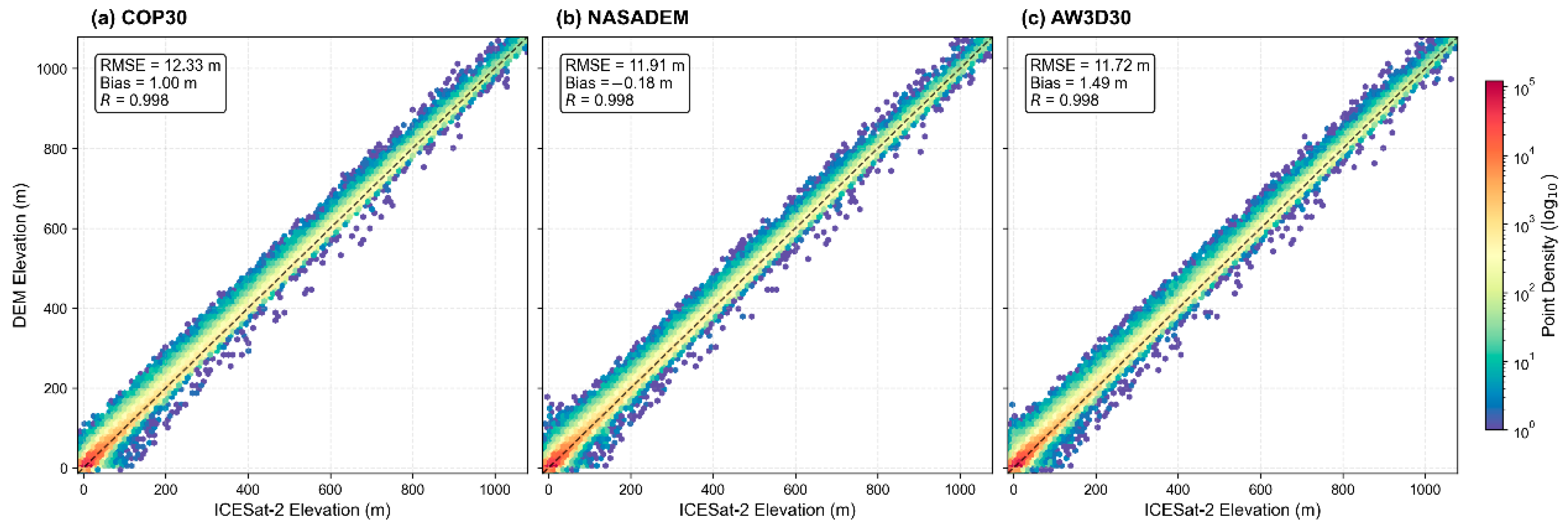
Scatter density plots (Figure 3) illustrate the overall consistency between the three global DEMs and ICESat-2. Visually, the elevation points for all three datasets are densely concentrated along the 1:1 diagonal line, demonstrating a strong linear relationship with the reference measurements. This observation is statistically supported by the Pearson correlation coefficient (R), which reached 0.998 for COP30, NASADEM, and AW3D30, indicating a high degree of agreement. Despite the similar correlation, slight variations were observed in the scatter metrics. As shown in the annotations of Figure 3, AW3D30 exhibited a bias of 1.49 m, whereas COP30 and NASADEM showed biases of 1.00 m and −0.18 m, respectively. The RMSE derived from the elevation comparison was lowest for AW3D30 (11.72 m), followed by NASADEM (11.91 m) and COP30 (12.33 m).
Figure 3.
Scatter density plots comparing DEM elevations with ICESat-2 reference data for (a) COP30, (b) NASADEM, and (c) AW3D30. The 1:1 line is shown in black dashed style.
To further quantify the vertical accuracy, detailed error statistics (dh = HDEM − HICESat-2) were calculated for the 970,178 validation points (Table 2). Unlike the elevation scatter metrics, the analysis of elevation differences reveals distinct performance hierarchies. NASADEM achieved the lowest RMSE (7.775 m) and MAE (4.256 m), suggesting a superior overall accuracy in representing terrain height among the three products. COP30 followed, with an RMSE of 8.559 m and an MAE of 4.307 m. In contrast, AW3D30 yielded the highest RMSE (9.001 m) and MAE (5.142 m). Regarding systematic deviations, all three DEMs exhibited a positive mean error (Bias), indicating a general tendency to overestimate terrain elevation. NASADEM showed the smallest bias (2.311 m), while AW3D30 showed the largest (3.979 m).
Table 2.
Statistical accuracy assessment of global DEMs against ICESat-2.
The robustness of the datasets was further evaluated using percentile-based metrics. While NASADEM outperformed others in standard error metrics (RMSE and LE90), COP30 demonstrated the lowest LE68 value (3.48 m) compared to NASADEM (3.804 m) and AW3D30 (4.612 m). This suggests that, while NASADEM has fewer extreme errors (lower LE90 of 9.897 m versus COP30’s 11.391 m), the core error distribution of COP30 is slightly more concentrated around the median.
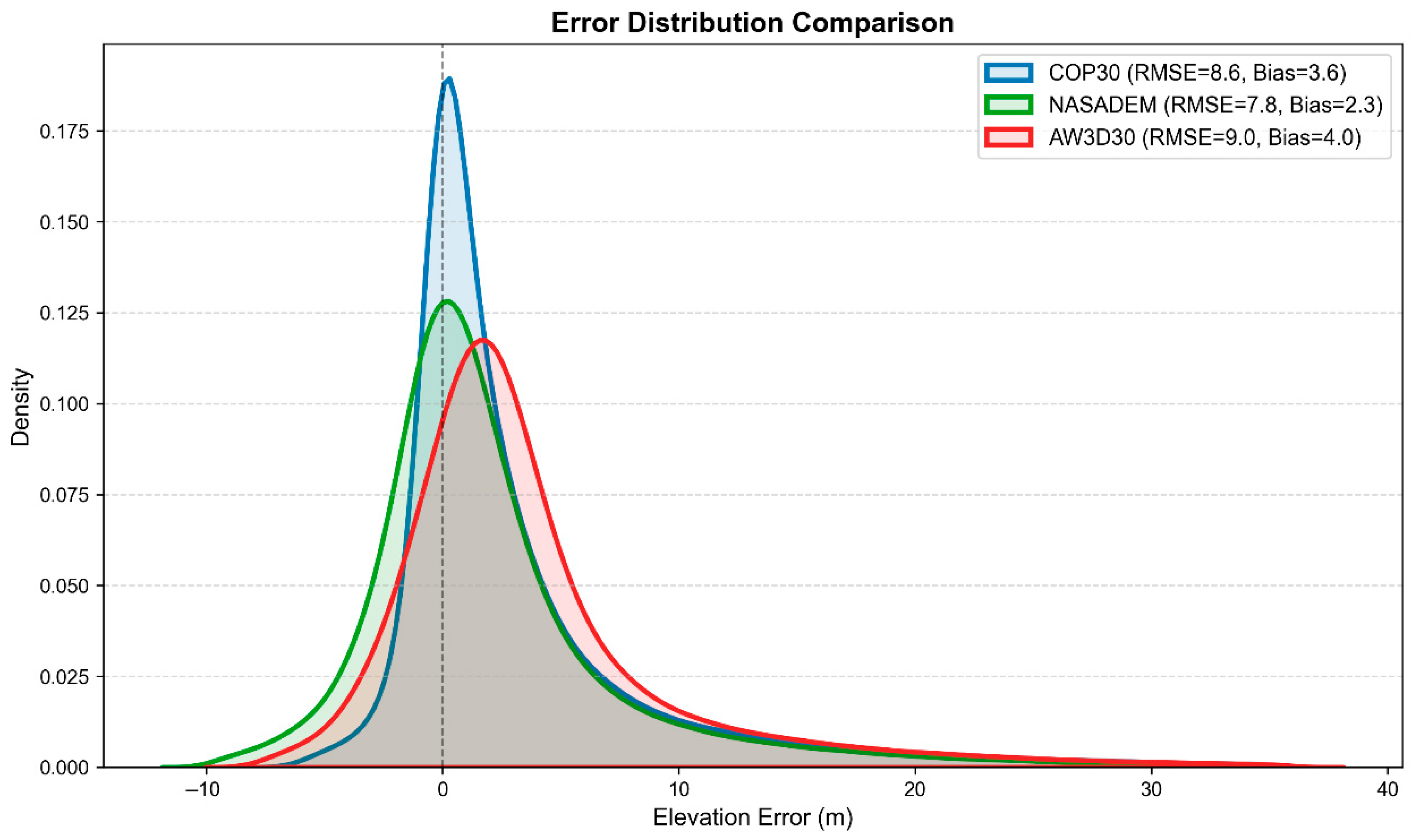
The morphology of the error distributions is visualized in Figure 4. All three DEMs exhibit a non-normal characteristic with a high concentration of values near the mean and distinctively long tails, indicating the presence of outliers. This deviation from normality is quantitatively supported by the high kurtosis values reported in Table 2 (ranging from 23.28 to 27.02). Visually, the error density curve for COP30 appears the narrowest and tallest. Rather than merely indicating a statistical concentration, this physically reflects COP30’s finer true spatial resolution. This finer resolution more closely aligns with the ~17 m footprint of the ICESat-2 reference data, thereby significantly reducing resolution-induced random matching noise. NASADEM shows a similarly sharp peak but with a slightly wider spread in the central range, while AW3D30 presents the shortest and widest distribution, reflecting its higher standard deviation (8.073 m) and larger dispersion of errors. The positive shift in the density peaks away from zero is consistent with the positive bias values observed across all datasets.
Figure 4.
Error distribution densities for the three global DEMs.
4.2. Global Feature Importance and Error Drivers
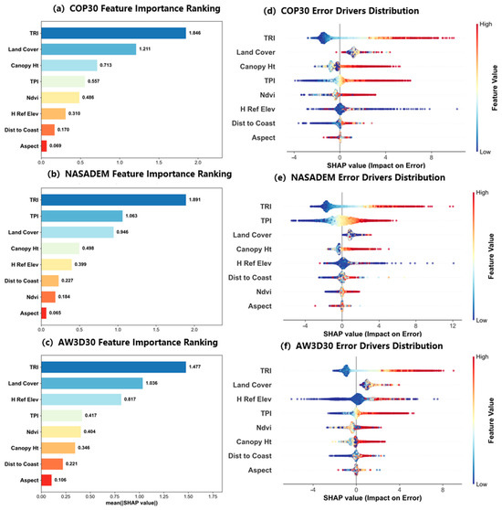
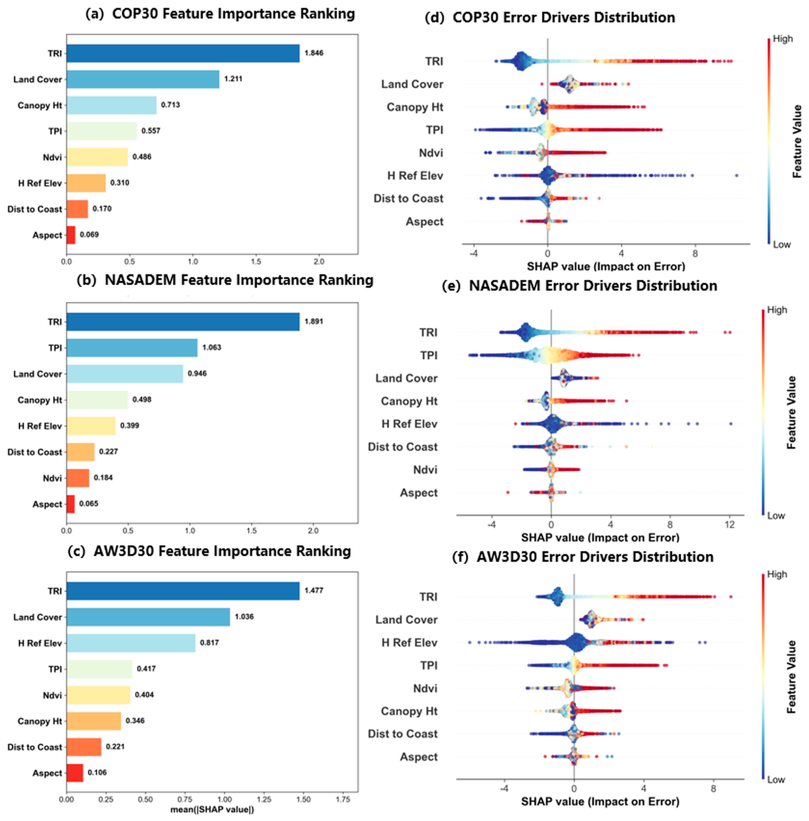
To identify the dominant factors governing the vertical accuracy of the three global DEMs, we analyzed the global feature importance using SHAP bar charts for quantitative ranking (Figure 5a–c) and beeswarm plots for impact visualization (Figure 5d–f). These plots reveal both the magnitude of each covariate’s contribution (mean absolute SHAP value) and the direction of their impact on the predicted error.
Figure 5.
SHAP-based model interpretability results. (a–c) Global feature importance ranking derived from mean absolute SHAP values. (d–f) SHAP summary plots visualizing the direction and magnitude of feature impacts, where color represents the feature value (red for high, blue for low).
The TRI emerged as the most critical determinant of elevation error across all three datasets, ranking first with mean absolute SHAP values of 1.846 (COP30), 1.891 (NASADEM), and 1.477 (AW3D30). The dependence patterns for TRI (Figure 5d–f) were highly consistent: high feature values (red dots) were predominantly concentrated on the positive side of the x-axis, while low values (blue dots) clustered on the negative side. This indicates a robust positive correlation between terrain roughness and elevation overestimation. In complex terrain with high TRI, both radar (COP30, NASADEM) and optical (AW3D30) sensors are prone to positive biases, likely due to geometric distortions (e.g., foreshortening, layover) in SAR data or matching failures/occlusions in optical stereo-pairs [36,37]. Conversely, the dense cluster of blue points (low TRI) suggests that, in flat terrain, these DEMs tend to exhibit a slight negative bias relative to the global mean error.
Following TRI, the categorically encoded Land Cover emerged as a universally dominant factor, ranking second for COP30 (1.211) and AW3D30 (1.036) and third for NASADEM (0.946). Notably, the SHAP beeswarm plots for Land Cover across all three DEMs exhibit a striking and consistent distribution: virtually all data points, regardless of their internal class coding, are clustered exclusively within the positive SHAP region. Because Land Cover is properly treated as a nominal categorical variable without numerical magnitude, this one-sided distribution physically implies that the presence of complex surface types—whether vegetation, built-up areas, or wetlands—systematically introduces positive elevation biases relative to bare earth baselines. This confirms that the physical structure of overlying surface features broadly impedes radar signal penetration and masks the true ground surface in optical imagery.
Beyond these shared dominant factors, each DEM exhibited unique secondary error drivers reflective of their specific sensor characteristics. For the X-band COP30 (Figure 5a,d), Canopy Height (0.713) ranked as the third most critical factor. The Canopy Height beeswarm plot exhibits a bimodal structure: a cluster near zero dominated by deep blue points (low canopy) and a cluster stretching into the positive axis dominated by deep red points (high canopy). This confirms that COP30 accurately represents bare ground but significantly overestimates elevation in tall vegetation due to the limited penetration of X-band signals [38].
For the C-band NASADEM (Figure 5b,e), TPI presents a unique error signature, ranking as the second most important feature (1.063). The TPI distribution in Figure 5e shows a clear separation: blue points (negative TPI, valleys) cluster on the negative SHAP side, while red points (positive TPI, ridges) cluster on the positive side. This implies a systematic morphological bias where NASADEM tends to underestimate elevations in valley bottoms and overestimate them on ridges.
The optical AW3D30 (Figure 5c,f) exhibits a fundamentally different error structure, with Reference Elevation (0.817) playing a pivotal role as the third most important feature. The beeswarm plot shows a distinct trend where low elevations (blue points) cluster near zero, while high elevations (red points) spread significantly towards the positive axis. This indicates an elevation-dependent error, where AW3D30 tends to overestimate terrain height in high-altitude regions, likely due to the challenges of stereo-matching [39].
4.3. Non-Linear Error Response to Topography and Vegetation
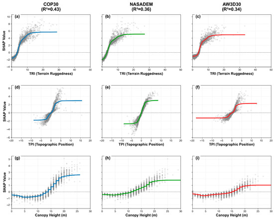
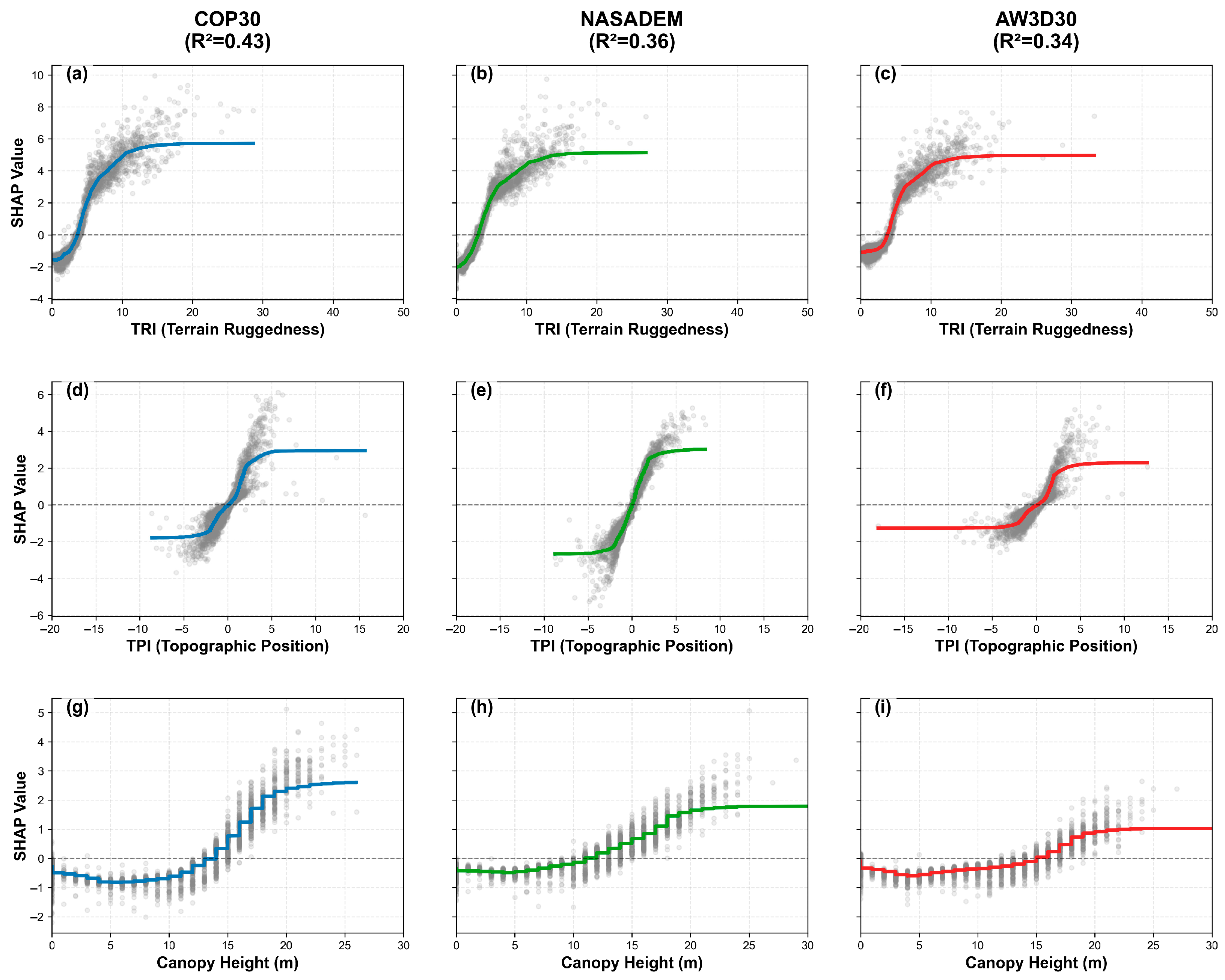
To investigate the detailed response of elevation errors to specific environmental gradients, SHAP dependence plots were generated for the three most influential continuous variables: TRI, TPI, and Canopy Height (Figure 6). As indicated in the figure annotations, the underlying XGBoost regression models (based on the full feature set) demonstrated varying degrees of overall explanatory power, with R2 values of 0.43 for COP30, 0.36 for NASADEM, and 0.34 for AW3D30. The notably higher R2 for COP30 suggests that its vertical errors are more systematically driven by the selected environmental covariates in this study. To distinguish the dominant signal from the scatter of individual samples, a smoothed trend line was superimposed on each plot, calculated using a rolling mean with a dynamic window size of 10% of the data points.
Figure 6.
SHAP dependence plots. (a–c) The impact of TRI on vertical error. (d–f) The impact of TPI on vertical error. (g–i) The impact of Canopy Height on vertical error.
The dependence of error on terrain ruggedness (Figure 6a–c) exhibits a consistent sigmoid-like pattern across all three global DEMs. In flat terrains (TRI < 5), the SHAP values generally remain in the negative territory, indicating a slight underestimation relative to the model baseline. A distinct transition occurs as TRI increases, where the trend line crosses from negative to positive, eventually stabilizing as a horizontal asymptote in highly rugged areas (TRI > 10). Despite the similar morphological trends, the magnitude of the bias in flat terrain varies by sensor. AW3D30 (Figure 6c) shows the most stable performance in low-relief zones, with its trend line intercept closest to zero. In contrast, NASADEM (Figure 6b) exhibits a notable negative deflection in flat areas, with the trend line starting near −2 m, suggesting a systematic underestimation in smooth terrains. COP30 (Figure 6a) falls between these two extremes. This implies that, while topographic complexity universally induces positive biases (likely due to foreshortening or occlusion), the baseline calibration in flat areas is best preserved in the optical AW3D30 product.
The response to TPI (Figure 6d–f) quantitatively captures the “smoothing effect” inherent in global DEMs. All three datasets show a sharp, linear transition within the TPI range of −5 to 5, where the error shifts rapidly from negative (in valleys) to positive (on ridges). Outside this transition zone, the impact tends to saturate. The severity of this smoothing effect is sensor-dependent. NASADEM (Figure 6e) displays the highest sensitivity, with SHAP values swinging dramatically from approximately −4 m in valleys to +4 m on ridges. This large dynamic range indicates a significant loss of high-frequency topographic detail, likely a legacy of the lower native resolution of the original SRTM data. COP30 (Figure 6d) shows a moderate range (−2 m to >2 m), while AW3D30 (Figure 6f) exhibits the most constrained error range (approximately −1 m to 2 m). The flatter slope of the AW3D30 trend line suggests that the optical stereo-photogrammetry method preserves peak–valley structures more faithfully than the interferometric radar techniques used for NASADEM and COP30.
The influence of vegetation height (Figure 6g–i) reveals a clear threshold behavior. For canopy heights below 10–15 m, the trend lines fluctuate gently within the negative or near-zero range, implying that low vegetation has minimal impact on the systematic error. However, as canopy height exceeds this 10–15 m threshold, the trend lines in all three plots cross into the positive y-axis and subsequently plateau, confirming the positive bias caused by the “canopy effect.” Among the three products, COP30 (Figure 6g) appears most susceptible to dense vegetation, with its trend line reaching the highest positive impact of approximately 3 m. NASADEM (Figure 6h) and AW3D30 (Figure 6i) show a comparatively lower saturation level, with maximum SHAP values hovering between 1 m and 2 m. The pronounced positive bias in COP30 is consistent with the limited penetration capability of X-band radar in dense forests, whereas the slightly lower bias in AW3D30 might be attributed to the specific processing algorithms used to generate the DSM, which may partially filter out canopy tops in certain stereo-matching scenarios.
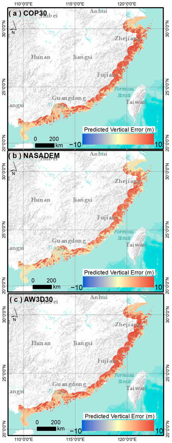
4.4. Spatial Distribution of Predicted Errors
Figure 7 visualizes the spatial heterogeneity of predicted vertical errors across the study area, rendered with a unified diverging color scale where warm tones (red) indicate overestimation, cool tones (blue) represent underestimation, and neutral yellow tones signify high accuracy (near-zero error). The dominant spatial theme across all three global DEMs is a widespread prevalence of positive bias, visualized as extensive red saturation throughout the inland regions. This systematic overestimation is spatially correlated with the rugged topography of the South China Hills (e.g., in Fujian and Guangdong provinces), where the combination of complex terrain and dense subtropical vegetation creates a challenging environment for satellite altimetry. The ubiquity of these positive errors corroborates the global feature importance analysis (Figure 5), confirming that terrain ruggedness and canopy cover act as the primary background constraints controlling the regional error budget, causing both radar foreshortening and stereo-occlusion regardless of the sensor technology.
Figure 7.
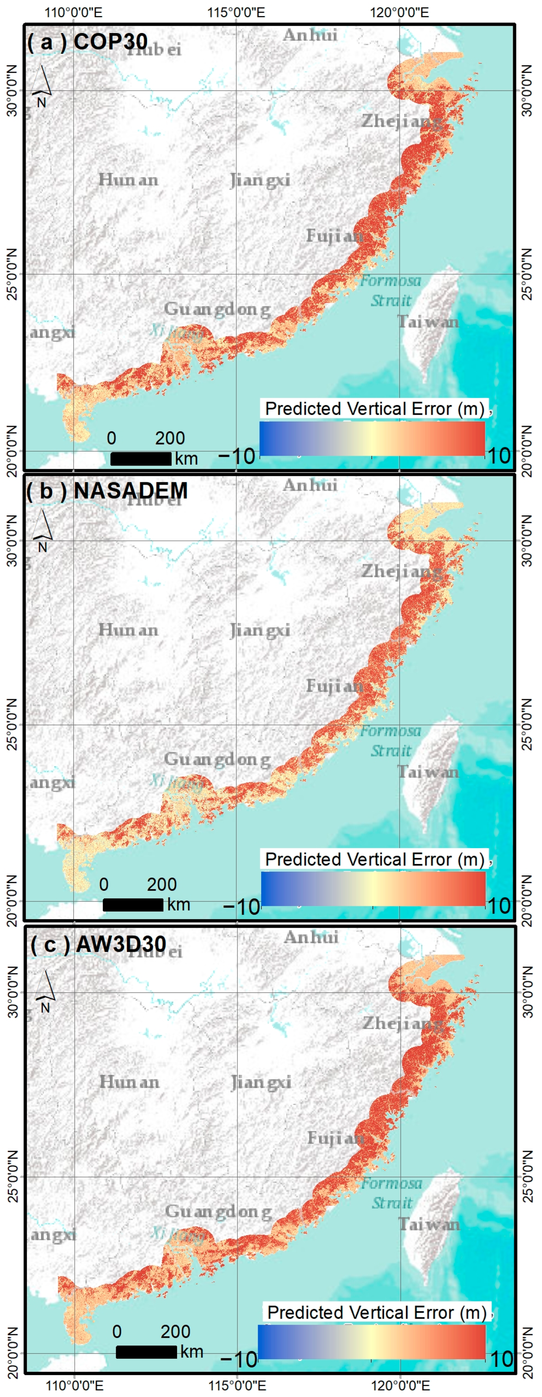
Spatial distribution of predicted vertical errors modeled by XGBoost.
Despite the dominance of positive errors in mountainous zones, distinct “islands of accuracy” emerge in the low-lying geomorphological units, specifically the Hangzhou Bay coastal plain in Northern Zhejiang, the Pearl River Delta in Guangdong, and the Leizhou Peninsula. In these regions, the error maps transition from saturated red to neutral yellow tones, indicating a significant reduction in vertical bias. Geomorphologically, these areas are characterized by flat alluvial deposits and are dominated by agriculture or urban settlements rather than the dense forests found in the highlands. The lack of tall canopy and topographic shading in these plains allows the digital surface models to align more closely with the bare-earth reference provided by ICESat-2, demonstrating that the vertical accuracy of global DEMs is highly sensitive to the transition from bedrock mountains to alluvial plains.
While all three products exhibit improved performance in these flat coastal zones compared to the highlands, distinct sensor-specific discrepancies are evident in the magnitude of the residual errors, manifested by the saturation of the “yellow” tones. NASADEM (Figure 7b) displays the faintest and most subtle yellow hues across the Hangzhou Bay and Pearl River Delta regions, visually indicating that its vertical deviations are minimal and closest to the zero-error baseline. This suggests that despite the global negative trend observed in the dependency plots, NASADEM achieves a remarkably high localized accuracy in these specific extensive alluvial plains, potentially benefitting from the effective removal of vegetation bias in agricultural zones during the SRTM reprocessing. In contrast, AW3D30 (Figure 7c) exhibits a deeper, more saturated yellow tone. This visual signature implies that, even in low-relief terrain, the optical AW3D30 retains a persistent, albeit reduced, positive bias (overestimation). This is likely attributable to the temporal mismatch and sensor characteristics [9,40]. The AW3D30 data, acquired between 2006 and 2011, captures the rapid urbanization of the Pearl River Delta, incorporating the height of dense buildings and infrastructure into the Digital Surface Model (DSM). When compared against ground-level reference points, this results in a positive error.
Conversely, NASADEM (Figure 7b), derived primarily from the SRTM in February 2000, represents an earlier landscape where many of these urbanized zones were likely agricultural plains or less developed. Furthermore, the inherent side-looking geometry and lower resolution of the original radar data, combined with the aggressive noise-smoothing algorithms applied during NASADEM reprocessing, tend to average out high-frequency surface features (such as individual buildings). Consequently, NASADEM presents a vertical profile that is statistically closer to the bare-earth surface in these specific rapidly developing floodplains, manifesting as the faintest “yellow” error patterns in the spatial map.
4.5. Practical Application: DEM Error Correction
While the primary objective of this study is to explain the physical drivers of DEM errors, the trained XGBoost models also possess significant practical engineering value for error correction. To demonstrate this capability, we applied the predicted vertical errors to correct the original DEM elevations in our independent testing set. The correction performance is summarized in Table 3. The results show a substantial reduction in RMSE across all three global DEMs. Notably, COP30 exhibited the most significant improvement, with its RMSE decreasing from 6.631 m to 4.368 m (a 34.12% improvement). NASADEM and AW3D30 also showed robust error reductions of 25.28% and 30.27%, respectively. These results confirm that our explainable machine learning framework is not only analytically insightful but also highly effective for operational topographic enhancement in complex coastal regions.
Table 3.
Summary of DEM vertical error correction using the XGBoost predictions.
Furthermore, to explicitly visualize the model’s actual fitting capability across the entire error spectrum, including its performance regarding heavy-tailed extreme outliers, scatter plots directly comparing the XGBoost-predicted vertical errors against the true errors for all three global DEMs are provided in Figure S2 in the Supplementary Materials. These distributions confirm that the model robustly captures the primary error trends without severe overfitting to extreme anomalies.
5. Discussion
5.1. Decomposition of Systematic and Random Errors
Beyond the individual feature analysis, the overall explainability of the XGBoost models provides critical insights into the fundamental error budget of global DEMs. Our models explain approximately 34% to 43% of the total error variance (R2 values of 0.43 for COP30, 0.36 for NASADEM, and 0.34 for AW3D30). While this suggests that a significant portion of the error remains unmodeled, this result aligns with the theoretical error partitioning of satellite altimetry systems.
The explained variance (approx. 0.4) represents the systematic error component driven by macroscopic terrain and environmental variables (e.g., slope, vegetation, and ruggedness). These are the deterministic biases that can be effectively learned and corrected by machine learning algorithms. The remaining unexplained variance (approx. 60%) is attributed to the inherent stochastic noise distinct to each sensor technology, which acts as a random noise floor independent of macroscopic terrain attributes.
For the SAR-based products (COP30 and NASADEM), this residual variance is primarily dominated by stochastic phase noise (speckle) and thermal noise inherent in interferometric processing [41]. In contrast, AW3D30 exhibits the lowest explainability (R2 ≈ 0.34), suggesting that its error budget is more heavily influenced by stochastic stereo-matching artifacts. These artifacts typically arise in low-texture areas (e.g., bright sand, water bodies) or cloud-shadowed regions, generating random geometric noise that correlates poorly with physical terrain attributes compared to the physics-based penetration errors observed in SAR DEMs.
This decomposition of error sources is consistent with established error budgets in the literature. For instance, in the validation of the SRTM, [42] demonstrated that, for continental-scale DEMs, the random error component (relative height error) accounts for approximately 60% of the total error budget (typically around 7.0 m), while systematic low-frequency errors (long-wavelength height error) account for the remaining 30–40% (4.0 m). Our findings corroborate this ratio, confirming that the XGBoost model has successfully captured the majority of the correctable systematic bias, while the residuals largely represent the irreducible random noise floor of the global DEMs. Furthermore, future studies should apply this explainable machine learning framework to more recent, high-resolution elevation models to determine whether the unmodeled random noise component (~60%) identified in this study can be significantly reduced.
While topographic complexity (e.g., TRI) broadly dominates DEM errors, the unique properties of the subtropical coastal zone introduce distinct localized error mechanisms. First, the land–sea transition creates sharp atmospheric water vapor gradients. The “Distance to Coast” covariate acts as a spatial proxy for these gradients, reflecting well-documented coastal tropospheric phase delays that introduce systemic artifacts in InSAR topographic mapping [43]. Second, the coastal interface features highly specific surface types, explicitly represented by our categorically encoded ESA WorldCover covariate (e.g., Classes 90 and 95). As extensively demonstrated in previous studies, these coastal surfaces induce unique elevation error patterns: wet tidal flats and wetlands (Class 90) often cause specular reflection and severe signal decoherence in radar and optical matching [4], while dense coastal mangroves (Class 95) exacerbate intense volume scattering, leading to systematic positive elevation biases (i.e., capturing the canopy phase center rather than bare earth) [44]. By directly incorporating these explicit land cover classes, our explainable model successfully accounts for the spatial heterogeneity driven by these coastal-specific physical mechanisms.
5.2. Comparison with Previous Studies and Limitations
Our statistical assessment ranks NASADEM as having the lowest overall RMSE (7.775 m), closely followed by COP30. This generally aligns with recent global validations, although differences in LE68 metrics highlight that COP30 often provides superior precision in non-extreme terrain. Numerous previous studies have extensively evaluated DEM quality across various global coastal zones and floodplains. For example, Ref. [4] performed rigorous statistical validations of the TanDEM-X DEM across selected global floodplain sites, highlighting general vegetation-induced biases, while [6] focused on quantifying the overall vertical accuracy and RMSE trends of newly released global DEMs (including Copernicus and NASADEM) in flood-prone environments [4,6]. While these conventional approaches provide vital baseline statistical validations, moving beyond them, the unique scientific contribution of this study lies in the operational attribution and correction of these errors by explicitly linking them to the fundamental acquisition modalities, geodetic baselines, and cartographic processing workflows inherent to each DEM. Because these intrinsic sensor properties fundamentally dictate how the measurement signal interacts with the ground, our analysis logically reveals a nuanced and universally dominant role of land surface characteristics in modulating vertical biases. While the SHAP dependence plots confirm a consistent threshold effect, indicating that all DSMs, regardless of sensor, fail to penetrate closed canopies (>15 m), the structural hierarchy of error drivers varies by sensor. For the X-band COP30 and optical AW3D30, categorically encoded Land Cover acts as a primary error driver (ranking second only to TRI). However, for the C-band NASADEM, topographic morphology (TPI) heavily modulates the errors alongside Land Cover. Furthermore, the distinct emergence of absolute elevation as a key driver for AW3D30 underscores its unique vulnerabilities. This distinction highlights that, while mitigating surface cover bias (e.g., vegetation removal) remains universally critical across all products, improving C-band and optical DEMs also heavily depends on addressing morphological smoothing (TPI) and elevation-dependent stereo-matching challenges, respectively.
A key finding is the anomalous topographic response of NASADEM. Classical literature on DEM generation posits that low-resolution DEMs suffer from a “smoothing effect” [45,46], typically causing underestimation on ridges (peak shaving) and overestimation in valleys (valley filling). Fundamentally, this smoothing is driven by the DEM’s true spatial resolution acting as a low-pass filter [20]. Contrary to this geometric theory, the SHAP summary plot (Figure 5e) reveals a distinct separation: positive TPI values (ridges, represented by red dots) cluster predominantly in the positive error domain, while negative TPI values (valleys, blue dots) cluster in the negative domain. This trend is further quantified by the dependence plot (Figure 6e), showing a dynamic range from −4 m to +4 m.
This discrepancy implies that geometric smoothing is not the sole dominant factor. On ridges, the “smoothing” signal is likely overpowered by surface characteristics (explicitly captured by our Land Cover and Canopy Height features). Because ridges in the subtropical study area are densely vegetated, the uncorrected C-band penetration bias (+5 to +10 m) dominates the geometric peak shaving (−2 to −3 m), resulting in a net positive error. Conversely, the underestimation in valleys is likely a byproduct of the hydro-flattening algorithms applied during NASADEM reprocessing. These algorithms, designed to enforce drainage connectivity, often “burn in” river networks, potentially lowering valley bottoms below the discrete point measurements of ICESat-2. This finding highlights that, for reprocessed DEMs like NASADEM, radiometric (vegetation) and procedural (hydro-enforcement) factors can outweigh purely geometric resolution effects.
Despite these insights, limitations remain. First, the temporal mismatch between the DEM generation (e.g., ~2000 for NASADEM, ~2010 for AW3D30) and the ICESat-2 acquisition (2019–present) introduces inevitable discrepancies, particularly in rapidly developing coastal zones as observed in the AW3D30 error maps. Over such a long period, the rapid urbanization, land reclamation, and infrastructure development characteristic of the Southeast China coastal zones (e.g., the Pearl River Delta and Hangzhou Bay) have substantially altered the surface topography. For instance, AW3D30 captures historical building heights from the late 2000s, which translates into localized positive vertical errors when compared to modern ICESat-2 bare-earth photons in areas that have since been redeveloped, reclaimed, or modified. Furthermore, natural canopy dynamics—such as forest growth, deforestation, or afforestation over the past 10 to 20 years—imply that the contemporary canopy height covariates may not perfectly represent the historical vegetation structure present during the initial radar or optical data acquisition. This temporal decoupling adds an inherent layer of temporal noise to the error evaluation and feature attribution, highlighting the need for time-synchronized elevation benchmarking in highly dynamic coastal environments. Second, the scale mismatch between the ICESat-2 footprint (~17 m) and the DEM pixel size (30 m) acts as a source of inherent random noise (matching artifacts) that our XGBoost model cannot fully resolve. Future work could integrate full-waveform LiDAR data to better decouple sub-pixel vegetation structure from terrain elevation.
Finally, it is important to address the spatial generalizability of our findings. While the empirical conclusions of this study are exclusively derived from the coastal zones of Zhejiang, Fujian and Guangdong provinces, this region serves as a highly representative natural laboratory for global coastal environments. The area features a complex intersection of rugged topography, dense subtropical forests, frequent monsoon cloud cover, and intense anthropogenic modifications. These extreme conditions are highly analogous to many rapidly developing coastal megaregions globally, particularly across Southeast Asia, the Global South, and other tropical/subtropical coastal belts. Consequently, the physical mechanisms of DEM errors identified in this explainable framework are expected to be highly transferable to similar global coastal environments. Future research should apply this framework to different climatic or geomorphological zones (e.g., arid coasts or high-latitude fjords) to further validate and expand upon these globally relevant error mechanisms.
6. Conclusions
This study established an explainable machine learning framework to decouple vertical errors in three 30 m global DEMs across the subtropical coastal zone of Southeast China. Validation against ICESat-2 reveals that NASADEM achieves the highest overall vertical accuracy (RMSE = 7.775 m), outperforming both COP30 and AW3D30 in this heterogeneous environment. While TRI and Land Cover act as the universally dominant error drivers, our XGBoost-SHAP analysis uncovered distinct, sensor-specific error mechanisms. Specifically, secondary to these shared effects, the X-band COP30 is notably susceptible to the “canopy effect” in forests exceeding 15 m, whereas the C-band NASADEM exhibits a unique topographic bias (driven by TPI) likely stemming from legacy hydro-flattening algorithms, and the optical AW3D30 is prone to elevation-dependent stereo-matching artifacts in complex terrain.
Furthermore, the error budget decomposition indicates that approximately 40% of the vertical error is systematic and correctable, driven by macroscopic terrain and surface factors, while the remaining ~60% represents irreducible stochastic sensor noise. These findings suggest that, while NASADEM offers the most robust baseline for this region, future accuracy enhancements for radar-based products must prioritize vegetation removal strategies, whereas optical DEM improvements rely on refining stereo-matching algorithms in high-relief areas.
Supplementary Materials
The following supporting information can be downloaded at: https://www.mdpi.com/article/10.3390/rs18081125/s1. Figure S1: Pearson correlation matrix heatmap of the continuous covariates used for vertical error modeling. The color gradient indicates the strength and direction of the linear correlation (r). A remarkably high positive correlation (r = 0.98) was identified between the Topographic Ruggedness Index (TRI) and Slope. To prevent the destabilization of SHAP value allocations caused by this severe multicollinearity, Slope was excluded from the final XGBoost models. Figure S2: Scatter plots comparing the XGBoost-predicted vertical errors against the true vertical errors for (a) COP30, (b) NASADEM, and (c) AW3D30. The direct comparison demonstrates the model’s robust fitting capability across the entire error spectrum, including its performance on heavy-tailed extreme outliers.
Author Contributions
Validation, X.L.; resources, F.T.; writing—original draft preparation, J.C., F.T. and H.L.; writing—review and editing, J.C., B.H. and X.L.; visualization, B.H.; supervision, H.L. All authors have read and agreed to the published version of the manuscript.
Funding
This research was funded by the Research Project on Representative Islands Platform for Resources, Ecology, and Sustainable Development (grant number 102121221620000009001), Ministry of Natural Resources 2024 Annual Ministry-Province Cooperation Projects (2024ZRBSHZ105) and Fujian Provincial Natural Science Foundation of China (No. 2023J01163741). The APC was funded by the Research Project on Representative Islands Platform for Resources, Ecology, and Sustainable Development and Ministry of Natural Resources 2024 Annual Ministry-Province Cooperation Projects.
Data Availability Statement
The data presented in this study are openly available in the OpenTopography platform (https://opentopography.org, accessed on 9 January 2026) and the National Snow and Ice Data Center (https://nsidc.org/data/icesat/data, accessed on 9 January 2026). Furthermore, the source code supporting the explainable machine learning analysis is openly available in the Zenodo repository at https://doi.org/10.5281/zenodo.18517740.
Acknowledgments
During the preparation of this manuscript, the authors used Gemini 3 for the purposes of language polishing. The authors have reviewed and edited the output and take full responsibility for the content of this publication.
Conflicts of Interest
The authors declare no conflicts of interest.
Abbreviations
The following abbreviations are used in this manuscript:
| DEM | Digital elevation model |
| ALOS | Advanced Land Observing Satellite |
| AW3D30 | ALOS World 3D-30 m |
| COP30 | Copernicus DEM |
| NASA | National Aeronautics and Space Administration |
| ATLAS | The advanced topographic laser altimeter system |
| NDVI | Normalized difference vegetation index |
| SAR | Synthetic aperture radar |
| SHAP | SHapley Additive exPlanations |
| XGBoost | eXtreme Gradient Boosting |
| RMSE | Root mean square error |
| TPI | Topographic position index |
| TRI | Terrain ruggedness index |
References
- Moore, I.D.; Grayson, R.B.; Ladson, A.R. Digital Terrain Modelling: A Review of Hydrological, Geomorphological, and Biological Applications. Hydrol. Process. 1991, 5, 3–30. [Google Scholar] [CrossRef] [Scilit]
- Coveney, S.; Roberts, K. Lightweight UAV Digital Elevation Models and Orthoimagery for Environmental Applications: Data Accuracy Evaluation and Potential for River Flood Risk Modelling. Int. J. Remote Sens. 2017, 38, 3159–3180. [Google Scholar] [CrossRef] [Scilit]
- Fattahi, H.; Amelung, F. DEM Error Correction in InSAR Time Series. IEEE Trans. Geosci. Remote Sens. 2013, 51, 4249–4259. [Google Scholar] [CrossRef] [Scilit]
- Hawker, L.; Neal, J.; Bates, P. Accuracy Assessment of the TanDEM-X 90 Digital Elevation Model for Selected Floodplain Sites. Remote Sens. Environ. 2019, 232, 111319. [Google Scholar] [CrossRef] [Scilit]
- Uuemaa, E.; Ahi, S.; Montibeller, B.; Muru, M.; Kmoch, A. Vertical Accuracy of Freely Available Global Digital Elevation Models (Aster, Aw3d30, Merit, Tandem-x, Srtm, and Nasadem). Remote Sens. 2020, 12, 3482. [Google Scholar] [CrossRef] [Scilit]
- Meadows, M.; Jones, S.; Reinke, K. Vertical Accuracy Assessment of Freely Available Global DEMs (FABDEM, Copernicus DEM, NASADEM, AW3D30 and SRTM) in Flood-Prone Environments. Int. J. Digit. Earth 2024, 17, 2308734. [Google Scholar] [CrossRef] [Scilit]
- Horritt, M.S.; Bates, P.D. Evaluation of 1D and 2D Numerical Models for Predicting River Flood Inundation. J. Hydrol. 2002, 268, 87–99. [Google Scholar] [CrossRef] [Scilit]
- Marsh, C.B.; Harder, P.; Pomeroy, J.W. Validation of FABDEM, a Global Bare-Earth Elevation Model, against UAV-Lidar Derived Elevation in a Complex Forested Mountain Catchment. Environ. Res. Commun. 2023, 5, 031009. [Google Scholar] [CrossRef] [Scilit]
- Li, H.; Zhao, J.; Yan, B.; Yue, L.; Wang, L. Global DEMs Vary from One to Another: An Evaluation of Newly Released Copernicus, NASA and AW3D30 DEM on Selected Terrains of China Using ICESat-2 Altimetry Data. Int. J. Digit. Earth 2022, 15, 1149–1168. [Google Scholar] [CrossRef] [Scilit]
- Carrera-Hernández, J.J. Not All DEMs Are Equal: An Evaluation of Six Globally Available 30 m Resolution DEMs with Geodetic Benchmarks and LiDAR in Mexico. Remote Sens. Environ. 2021, 261, 112474. [Google Scholar] [CrossRef] [Scilit]
- Saksena, S.; Merwade, V. Incorporating the Effect of DEM Resolution and Accuracy for Improved Flood Inundation Mapping. J. Hydrol. 2015, 530, 180–194. [Google Scholar] [CrossRef] [Scilit]
- Simard, M.; Denbina, M.; Marshak, C.; Neumann, M. A Global Evaluation of Radar-Derived Digital Elevation Models: SRTM, NASADEM, and GLO-30. J. Geophys. Res. Biogeosci. 2024, 129, e2023JG007672. [Google Scholar] [CrossRef] [Scilit]
- Li, M.; Yin, X.; Tang, B.H.; Yang, M. Accuracy Assessment of High-Resolution Globally Available Open-Source DEMs Using ICESat/GLAS over Mountainous Areas, A Case Study in Yunnan Province, China. Remote Sens. 2023, 15, 1952. [Google Scholar] [CrossRef] [Scilit]
- Lundberg, S.M.; Lee, S.I. A Unified Approach to Interpreting Model Predictions. In Proceedings of the Advances in Neural Information Processing Systems, Long Beach, CA, USA, 4–9 December 2017. [Google Scholar]
- Shi, N.; Li, Y.; Wen, L.; Zhang, Y. Rapid Prediction of Landslide Dam Stability Considering the Missing Data Using XGBoost Algorithm. Landslides 2022, 19, 2951–2963. [Google Scholar] [CrossRef] [Scilit]
- Wang, H.; Liu, L.; Yin, L.; Shen, J.; Li, S. Exploring the Complex Relationships and Drivers of Ecosystem Services across Different Geomorphological Types in the Beijing-Tianjin-Hebei Region, China (2000–2018). Ecol. Indic. 2021, 121, 107116. [Google Scholar] [CrossRef] [Scilit]
- Wang, M.; Li, Y.; Yuan, H.; Zhou, S.; Wang, Y.; Adnan Ikram, R.M.; Li, J. An XGBoost-SHAP Approach to Quantifying Morphological Impact on Urban Flooding Susceptibility. Ecol. Indic. 2023, 156, 111137. [Google Scholar] [CrossRef] [Scilit]
- You, J.; Yin, F.; Zhang, B.; Zhou, M.; Qing, Y.; Chen, Y.; Gao, L. A Novel Environmental Nndicator: Compound Wind Droughts and Heat Waves for Assessing Climate-Driven Ecological and Energy Sustainability. Ecol. Indic. 2025, 178, 114114. [Google Scholar] [CrossRef] [Scilit]
- Cheshmehzangi, A.; Tang, T. Guangdong-Fujian-Zhejiang Coastal Region: A Network Corridor Between Three Coastal Provinces. In China’s City Cluster Development in the Race to Carbon Neutrality; Springer Nature: Singapore, 2022. [Google Scholar]
- Guth, P.L.; Van Niekerk, A.; Grohmann, C.H.; Muller, J.P.; Hawker, L.; Florinsky, I.V.; Gesch, D.; Reuter, H.I.; Herrera-Cruz, V.; Riazanoff, S.; et al. Digital Elevation Models: Terminology and Definitions. Remote Sens. 2021, 13, 3581. [Google Scholar] [CrossRef] [Scilit]
- Tadono, T.; Takaku, J.; Tsutsui, K.; Oda, F.; Nagai, H. Status of “ALOS World 3D (AW3D)” Global DSM Generation. In Proceedings of the International Geoscience and Remote Sensing Symposium (IGARSS), Milan, Italy, 26–31 July 2015. [Google Scholar]
- Crippen, R.; Buckley, S.; Agram, P.; Belz, E.; Gurrola, E.; Hensley, S.; Kobrick, M.; Lavalle, M.; Martin, J.; Neumann, M.; et al. Nasadem Global Elevation Model: Methods and Progress. Int. Arch. Photogramm. Remote Sens. Spat. Inf. Sci. 2016, XLI-B4, 125–128. [Google Scholar] [CrossRef] [Scilit]
- Neumann, T.A.; Martino, A.J.; Markus, T.; Bae, S.; Bock, M.R.; Brenner, A.C.; Brunt, K.M.; Cavanaugh, J.; Fernandes, S.T.; Hancock, D.W.; et al. The Ice, Cloud, and Land Elevation Satellite—2 Mission: A Global Geolocated Photon Product Derived from the Aadvanced Ttopographic Llaser Aaltimeter Ssystem. Remote Sens. Environ. 2019, 233, 111325. [Google Scholar] [CrossRef] [Scilit]
- Xiang, J.; Li, H.; Zhao, J.; Cai, X.; Li, P. Inland Water Level Measurement from Spaceborne Laser Altimetry: Validation and Comparison of Three Missions over the Great Lakes and Lower Mississippi River. J. Hydrol. 2021, 597, 126312. [Google Scholar] [CrossRef] [Scilit]
- Malashin, R.; Mikhalkova, M. Method for Sharpening Combined Stereo Images in the Presence of Optical Distortions. J. Opt. Technol. 2023, 90, 444–450. [Google Scholar] [CrossRef] [Scilit]
- Wang, Z.; Ma, X.; Peng, J.; Shi, M.; Peng, Y.; Su, Y.; Guo, Z.; Wang, W. Quantitative Analysis of SAR Image Geometric Distortion and Its Application in Deformation Rate Fusion Mapping. IEEE J. Sel. Top. Appl. Earth Obs. Remote Sens. 2024, 17, 3780–3790. [Google Scholar] [CrossRef] [Scilit]
- Shawn, R.; Degloria, S.D.; Elliot, R. A Terrain Ruggedness Index That Quantifies Topographic Heterogeneity. Intermt. J. Sci. 1999, 5, 23–27. [Google Scholar]
- Weiss, A.D. Topographic Position and Landforms Analysis, The Nature Conservancy. In Proceedings of the Poster Presentation, ESRI User Conference, San Diego, CA, USA, 9–13 July 2001; Volume 64. [Google Scholar]
- Hancock, G.R.; Martinez, C.; Evans, K.G.; Moliere, D.R. A Comparison of SRTM and High-Resolution Digital Elevation Models and Their Use in Catchment Geomorphology and Hydrology: Australian Examples. Earth Surf. Process. Landf. 2006, 31, 1394–1412. [Google Scholar] [CrossRef] [Scilit]
- Bekaert, D.P.S.; Walters, R.J.; Wright, T.J.; Hooper, A.J.; Parker, D.J. Statistical Comparison of InSAR Tropospheric Correction Techniques. Remote Sens. Environ. 2015, 170, 40–47. [Google Scholar] [CrossRef] [Scilit]
- Lang, N.; Jetz, W.; Schindler, K.; Wegner, J.D. A High-Resolution Canopy Height Model of the Earth. Nat. Ecol. Evol. 2023, 7, 1778–1789. [Google Scholar] [CrossRef] [Scilit] [PubMed]
- Chaaban, F.; El Khattabi, J.; Darwishe, H. Accuracy Assessment of ESA WorldCover 2020 and ESRI 2020 Land Cover Maps for a Region in Syria. J. Geovisualization Spat. Anal. 2022, 6, 31. [Google Scholar] [CrossRef] [Scilit]
- Ogino, S.Y.; Yamanaka, M.D.; Mori, S.; Matsumoto, J. Tropical Coastal Dehydrator in Global Atmospheric Water Circulation. Geophys. Res. Lett. 2017, 44, 11–636. [Google Scholar] [CrossRef] [Scilit]
- Zou, G.X.; Tong, C.; Sun, H.L.; Peng, P. Research on Electromagnetic Scattering Characteristics of Combined Conducting and Dielectric Target above Coastal Environment. IEEE Access 2020, 8, 169286–169303. [Google Scholar] [CrossRef] [Scilit]
- Höhle, J.; Höhle, M. Accuracy Assessment of Digital Elevation Models by Means of Robust Statistical Methods. ISPRS J. Photogramm. Remote Sens. 2009, 64, 398–406. [Google Scholar] [CrossRef] [Scilit]
- Samuele, D.P.; Filippo, S.; Orusa, T.; Enrico, B.M. Mapping SAR Geometric Distortions and Their Stability along Time: A New Tool in Google Earth Engine Based on Sentinel-1 Image Time Series. Int. J. Remote Sens. 2021, 42, 9135–9154. [Google Scholar] [CrossRef] [Scilit]
- Liu, H.H.; Zhao, Y.J.; Wang, L.; Liu, Y.Y. Comparison of DEM Accuracies Generated from Different Stereo Pairs over a Plateau Mountainous Area. J. Mt. Sci. 2021, 18, 1580–1590. [Google Scholar] [CrossRef] [Scilit]
- Xu, K.; Zhao, L.; Chen, E.; Li, K.; Liu, D.; Li, T.; Li, Z.; Fan, Y. Forest Height Estimation Approach Combining P-Band and X-Band Interferometric SAR Data. Remote Sens. 2022, 14, 3070. [Google Scholar] [CrossRef] [Scilit]
- Purinton, B.; Bookhagen, B. Beyond Vertical Point Accuracy: Assessing Inter-Pixel Consistency in 30 m Global DEMs for the Arid Central Andes. Front. Earth Sci. 2021, 9, 758606. [Google Scholar] [CrossRef] [Scilit]
- Li, H.; Zhao, J. Evaluation of the Newly Released Worldwide AW3D30 DEM over Typical Landforms of China Using Two Global DEMs and ICESat/GLAS Data. IEEE J. Sel. Top. Appl. Earth Obs. Remote Sens. 2018, 11, 2874361. [Google Scholar] [CrossRef] [Scilit]
- Rizzoli, P.; Martone, M.; Gonzalez, C.; Wecklich, C.; Borla Tridon, D.; Bräutigam, B.; Bachmann, M.; Schulze, D.; Fritz, T.; Huber, M.; et al. Generation and Performance Assessment of the Global TanDEM-X Digital Elevation Model. ISPRS J. Photogramm. Remote Sens. 2017, 132, 119–139. [Google Scholar] [CrossRef] [Scilit]
- Farr, T.G.; Rosen, P.A.; Caro, E.; Crippen, R.; Duren, R.; Hensley, S.; Kobrick, M.; Paller, M.; Rodriguez, E.; Roth, L.; et al. The Shuttle Radar Topography Mission. Rev. Geophys. 2007, 45, RG2004. [Google Scholar] [CrossRef] [Scilit]
- Zebker, H.A.; Rosen, P.A.; Hensley, S. Atmospheric Effects in Interferometric Synthetic Aperture Radar Surface Deformation and Topographic Maps. J. Geophys. Res. Solid Earth 1997, 102, 7547–7563. [Google Scholar] [CrossRef] [Scilit]
- Simard, M.; Rivera-Monroy, V.H.; Mancera-Pineda, J.E.; Castañeda-Moya, E.; Twilley, R.R. A Systematic Method for 3D Mapping of Mangrove Forests Based on Shuttle Radar Topography Mission Elevation Data, ICEsat/GLAS Waveforms and Field Data: Application to Ciénaga Grande de Santa Marta, Colombia. Remote Sens. Environ. 2008, 112, 2131–2144. [Google Scholar] [CrossRef] [Scilit]
- Hayakawa, Y.S.; Oguchi, T.; Lin, Z. Comparison of New and Existing Global Digital Elevation Models: ASTER G-DEM and SRTM-3. Geophys. Res. Lett. 2008, 35, 17404–17405. [Google Scholar] [CrossRef] [Scilit]
- Jarvis, A.; Rubiano, J.; Nelson, A.; Farrow, A.; Mulligan, M. Practical Use of SRTM Data in the Tropics—Comparisons with Digital Elevation Models Generated from Cartographic Data. Trop. Agric. 2004, 198, 1–32. [Google Scholar]

Disclaimer/Publisher’s Note: The statements, opinions and data contained in all publications are solely those of the individual author(s) and contributor(s) and not of MDPI and/or the editor(s). MDPI and/or the editor(s) disclaim responsibility for any injury to people or property resulting from any ideas, methods, instructions or products referred to in the content. |
© 2026 by the authors. Licensee MDPI, Basel, Switzerland. This article is an open access article distributed under the terms and conditions of the Creative Commons Attribution (CC BY) license.