


Highlights
What are the main findings?
- A two-stage anomaly detection framework following “temporal physical pre-screening first, spatial statistical verification later” is proposed, effectively integrating diurnal variation constraints and spatial consistency checks.
- The method significantly outperforms STL and double standardization, achieving average improvement rates of 23.61%, 18.79%, 16.46%, and 61.33% in RMSE, MAE, R, and R2, respectively, on hourly LST data from the Heihe River Basin.
What are the implications of the main findings?
- It provides a physically interpretable and operationally robust solution for quality control of high-temporal-resolution LST data, enhancing reliability in complex land surface thermal infrared scenarios.
- By prioritizing the reduction of “mis-correction” risk, the method is particularly suitable for applications demanding high physical consistency, such as energy balance analysis and trend studies.
Abstract
High-spatiotemporal-resolution land surface temperature (LST) data are crucial for analyzing surface energy balance, modeling temperature-related processes, and monitoring thermal environments. However, despite advancements in multi-source fusion and reconstruction techniques, high-frequency LST data remain susceptible to anomalies such as abrupt changes and outliers due to retrieval uncertainties and varying observation conditions. Conventional statistical outlier detection methods risk misidentifying physically plausible rapid weather changes as data errors, introducing systematic biases. To address this, we propose a two-stage anomaly detection framework that follows a “temporal physical pre-screening first, spatial statistical verification later” logic. First, a piecewise empirical model, based on typical diurnal LST variation characteristics, is constructed to identify points violating physical patterns. Subsequently, a spatial consistency test using median absolute deviation (MAD) is introduced to distinguish real weather-driven fluctuations from genuine data anomalies from a spatial synergy perspective. This sequential design effectively reduces the risk of mis-correcting physically reasonable temperature variations. Validated using hourly seamless LST data (2016–2021) and ground observations in the Heihe River Basin, our method outperformed Seasonal-Trend decomposition using Loess (STL), double standardization methods, and robust Holt–Winters. For over 87% of the detected anomalies, the proposed method demonstrated positive improvement rates in RMSE, MAE, R, and R2. The overall average improvement rates reached 23.61%, 18.79%, 16.46%, and 61.33%, respectively, indicating robust performance. The results underscore that explicitly incorporating physical constraints enhances the reliability and interpretability of quality control for high-temporal-resolution remote sensing LST data.
1. Introduction
With the increasing demand for precision in early forest fire detection, urban heat environment assessment, and permafrost monitoring, spaceborne thermal infrared remote sensing technology is rapidly evolving towards high spatiotemporal resolution, all-weather capability, and intelligence [1,2,3,4]. Breakthroughs in the spatiotemporal resolution and quantitative capabilities of new-generation Earth observation systems have made continuous and dynamic monitoring of surface thermal processes possible [5,6]. In this context, enhancing the quantitative modeling capability for complex land surface thermal infrared scenes is of great significance for linking sensor design, physical retrieval, and scientific applications [7].
Land surface temperature (LST) is a key physical parameter characterizing land surface thermal infrared scenes. It is closely coupled with processes such as evapotranspiration, soil moisture, and vegetation status and is widely used in studies on urban heat islands, drought monitoring, ecosystem modeling, and climate change [8,9,10,11,12,13,14]. In recent years, developments in multi-source data fusion and reconstruction techniques have facilitated various high-continuity LST products, significantly enhancing the capacity for regional thermal process simulation and long-term trend analysis [15,16,17]. By integrating passive microwave data, reanalysis data, and physical models, some products have improved all-weather LST product quality while maintaining high temporal coverage [18,19,20,21].
However, influenced by multiple factors such as the inherent limitations of model parameterization [22], uncertainties in bias correction methods, theoretical assumption constraints of multi-source data fusion algorithms [23], “phase lags” between multi-source data [24], and physical definition differences between observations and simulations, high-spatiotemporal-resolution LST products inevitably still contain anomalies like abrupt changes, outliers, or trend breaks. If not identified and processed, these anomalies can disrupt the physical consistency of time series, leading to issues such as biases in energy balance estimation, misjudgment of thermal anomalies, and instability in trend analysis. Therefore, developing highly robust anomaly detection methods for high-spatiotemporal-resolution LST data has become a critical step in enhancing data quality.
Currently, anomaly detection methods for meteorological and remote sensing time series mainly fall into three categories: statistical methods, machine learning, and deep learning. Statistical methods (e.g., Seasonal-Trend decomposition using Loess (STL) [25,26] and double standardization methods [27]) are structurally simple and computationally efficient, having been widely applied in the quality control of ground weather stations and historical temperature series. Various machine learning methods can, to some extent, capture the complex spatial distribution and nonlinear relationships of multi-station temperature fields, demonstrating performance superior to traditional spatial regression and Inverse Distance Weighting (IDW) in spatial quality control and interpolation for station networks [28]. Deep learning models, by virtue of their theoretical strength in nonlinear fitting and automatic feature extraction, are particularly suited for large-scale, multivariate time series data analysis [29]. Nevertheless, current methods face notable challenges when dealing with high-temporal-frequency LST data characterized by strong non-stationarity, significant feature uncertainty, and difficulty in sample selection: statistical methods are sensitive to parameter settings and prone to false deletions or missed detections; machine learning methods rely on feature engineering and regional parameter tuning, which limits their generalizability; and deep learning methods require large sample sizes and suffer from weak interpretability. For hourly high-temporal-frequency LST data series, there is currently a lack of a systematic anomaly identification framework that balances physical rationality and detection robustness, which constrains the in-depth application of such data in refined thermal environment analysis.
Many studies have primarily focused on improving the accuracy of single detection algorithms applied solely to either the temporal or spatial dimension, with comparatively less attention paid to the detection structure and process that integrates spatiotemporal correlations [27,30]. Most existing methods formally adopt a single-stage, symmetric detection logic. In this approach, anomalies are directly determined within a single step based on the degree of statistical deviation in both time and space. This does not differentiate between the levels of preliminary screening and final confirmation, nor does it prioritize the physical laws of the temporal dimension [27,30,31]. When processing high-frequency hourly land surface temperature data, this approach has significant limitations. On one hand, the diurnal variation in LST is radiation-dominated and exhibits strong periodicity. On the other hand, rapid weather processes can lead to fluctuations that are physically reasonable but statistically anomalous [16,32]. This makes it difficult for traditional methods based on a single statistical anomaly criterion to effectively distinguish between real weather changes and data errors [30]. Therefore, this paper proposes a sequential two-stage detection framework. Its core contribution is not an improvement to a single detection method, but a reconstruction of the anomaly detection process. The fundamental difference between this work and existing spatiotemporal anomaly detection methods lies in the following: instead of attempting to compromise between missed detections and false alarms using a single threshold or a unified discriminant function, it decouples these two types of risk through an asymmetric, sequential decision-making process. These risks are then independently managed by physical constraints and spatial constraints, respectively.
To tackle these challenges, this paper proposes a two-stage anomaly detection framework following the principle of “temporal physical pre-screening first, spatial statistical verification later”. First, an empirical model based on the physical characteristics of LST diurnal variation is constructed for preliminary temporal screening (Section 3), prioritizing the retention of temporal variations conforming to physical laws. Subsequently, a spatial consistency test is introduced to filter and finally confirm the genuine anomalies from the preliminary candidates. This sequential design aims to reduce the risk of mis-deleting real weather changes due to statistical outliers from the outset, thereby enhancing the physical rationality and robustness of anomaly identification. Utilizing multi-year, multi-site observed land surface temperature series data from the Heihe River Basin (Section 2), we systematically validate the proposed method’s effectiveness in anomaly identification and correction. In addition, we conduct a comparative analysis with the STL and double standardization methods (Section 4) to evaluate their performance in practical applications. This method provides a physically interpretable and operationally robust solution for the quality control of high-temporal-frequency LST data, contributing to improved reliability and applicability of the data in complex land surface thermal infrared scenarios.
2. Selection and Analysis of Research Data
2.1. Hourly LST Dataset
The hourly LST data used in this study were sourced from the 0.02° seamless hourly land surface temperature dataset over East Asia (2016–2021) [23,33]. This product utilizes Himawari-8/Advanced Himawari Imager (AHI) thermal infrared observations as the core data source and combines the iTES retrieval algorithm, bias correction techniques, and the Multiresolution Kalman Filter (MKF) method to achieve dynamic optimal fusion of multi-source data. The product features a high temporal resolution of 1 h and a spatial resolution of approximately 2 km. It maintains good data continuity under both clear-sky and partially cloudy conditions, making it suitable for hourly monitoring and modeling analysis of land surface thermal processes. The main attributes of the dataset are summarized in Table 1.
Table 1.
Attribute summary of the 0.02° seamless hourly land surface temperature dataset over East Asia (2016–2021).
2.2. Ground Observation Data
The Heihe River Basin Integrated Observatory Network covers various typical underlying surface types, including alpine meadows, oasis farmlands, desert, wetlands, and shrub forests. It exhibits significant water–ecology–climate interactions, making it an ideal test area for validating remote sensing LST products [35]. This study selected seven long-term, continuously operational ground observation stations within the Heihe River Basin (http://data.tpdc.ac.cn) [36,37], as shown in Table 2. The geographical distribution of these stations is shown in Figure 1. The land surface temperature () observed at the stations was calculated from upwelling and downwelling longwave radiation data using the following formula:
where is the station-measured land surface temperature in Kelvin (K), and are the measured upwelling and downwelling longwave radiation at the station in , is broadband emissivity, obtained in this study from the Global Land Surface Satellite (GLASS) Broadband Emissivity product (spatial resolution: 1 km, temporal resolution: 8 days) [38,39,40], and σ is the Stefan–Boltzmann constant (5.67 × 10⁻⁸ W/(m2·K4)).
Table 2.
Overview of the ground validation sites.
Figure 1.
Distribution of ground validation sites in the Heihe River Basin. The numbers 1–7 correspond to the sites listed in Table 2.
To test the applicability of the proposed method in other regions, this study selected Huailai Station in the Haihe River Basin, located in the transitional zone between the North China Plain and mountainous areas, as an independent validation site. The underlying surface of this station is a single-cropping corn field, and its climate is classified as temperate sub-humid continental, which differs significantly from the arid/semi-arid conditions of the Heihe River Basin sites. The geographical location of the station is shown in Figure 2 [41,42,43].
Figure 2.
Geographical location of Huailai Station in the Haihe River Basin.
Due to systematic differences in physical meaning, sensor characteristics, and spatial representativeness between remotely sensed LST and the infrared radiometric temperature obtained from ground stations, previous work has commonly reported a stable absolute bias between the two time series, while their diurnal variation phase and relative patterns remain highly consistent [44,45,46,47,48,49,50]. Under strict quality control conditions, the station radiometric temperature and remotely sensed LST show high synchrony at the hourly scale. Therefore, these sites provide a reliable physical baseline for evaluating LST anomalies.
To assess the consistency in temporal patterns between the original remote sensing LST data and the station-observed land surface temperature, we calculated the correlation coefficient (R) for 14,589 valid days across the seven sites in the Heihe River Basin from 2016 to 2021. Statistical analysis (Figure 3) indicates that the remote sensing LST and station observation sequences exhibit highly synchronous diurnal variation patterns on the vast majority of days, with an overall average correlation coefficient as high as 0.95 and with over 90.20% of days having an R value above 0.90.
Figure 3.
(a) Histogram of correlation coefficient (R) distribution; (b) average correlation coefficient for different sites.
The distribution of R values shows excellent overall data quality, with approximately 74.32% of days falling within the extremely high correlation range (R ≥ 0.95). However, the analysis also identified a very small number of anomalies: a total of 7 days (0.048%) showed a negative correlation (R < 0), and a few other days exhibited a weak correlation.
3. Methodology
3.1. Typical Anomaly Types
Pixel-level time series analysis of the hourly LST sequences from 2016 to 2021 identified two representative types of anomalous features, as shown in Figure 4. Both types can cause significant interference to time series modeling and spatial analysis and, therefore, require effective identification and correction.
Figure 4.
Examples of anomaly types in remote sensing LST and ground station temperature time series: (a) single-point spike anomaly on 29 April 2017 (site S1); (b) single-point spike anomaly on 4 October 2016 (site S7); (c) continuous segment anomaly on 27 November 2016 (site S5); (d) mixed anomalies on 21 January 2018 (site S2). The red star denotes the identified spatiotemporal anomaly point, and the red dashed line indicates the deviation between the continuous anomalous LST curve and the station temperature curve.
Single-point Spike Anomaly: This is manifested as a sudden, sharp peak or drop in temperature at a specific moment, exhibiting an extreme difference from preceding and following time points.
Continuous Segment Anomaly: This is manifested as a systematic deviation of LST from the ground observation trend over a period of time.
3.2. General Idea and Framework
Anomaly detection in time series is of great importance in the quality control of remote sensing data. Owing to their intuitive methodologies and high computational efficiency, statistical approaches are extensively employed for this purpose. Classical methods such as Seasonal-Trend decomposition using Loess (STL) and the double standardization method have demonstrated good robustness in various time series scenarios: STL identifies anomalies by decomposing a time series into trend, seasonal, and residual components and detecting outliers within the residuals; the double standardization method performs standardization in both the temporal and spatial dimensions, respectively, and identifies anomalies based on set thresholds. In addition, the robust Holt–Winters method, a classic robust filtering technique, effectively mitigates the impact of outliers on trend and seasonal component estimation by recursively updating and cleaning observations in real time. However, STL is sensitive to seasonal period length and smoothing parameters, making it difficult to accurately characterize diurnal variation features at an hourly scale. Furthermore, although the double standardization method considers both temporal and spatial information, it is essentially a global outlier detection method and struggles to distinguish between different anomaly types. Although the robust Holt–Winters method can mitigate the impact of anomalies, it is still a purely temporal statistical method that lacks spatial information constraints, making it difficult to distinguish between real weather fluctuations and data errors.
To address the aforementioned shortcomings, this paper proposes a two-stage anomaly detection method following a “temporal first, spatial later” sequence, based on the physical mechanisms of temperature change. This method first conducts preliminary screening of anomalies based on physical constraints within the time series, followed by further verification through spatial statistical testing. Compared to the traditional approach that directly identifies anomalies based on outlier characteristics, this design can effectively distinguish between genuine weather events that are “physically plausible but statistically outliers” and data errors that are “physically implausible and spatially incoherent,” thereby systematically reducing the risk of misjudgment. This study follows a technical framework of “data input → anomaly point detection → anomaly point correction → method evaluation.” The overall research framework is illustrated in Figure 5.
Figure 5.
Overall research approach and framework. The dashed line demarcates the two core stages of the anomaly detection module: the upper temporal dimension pre-screening and the lower spatial consistency verification.
3.3. Two-Stage Anomaly Detection Method
3.3.1. Temporal Anomaly Pre-Screening: Empirical Model Based on Diurnal Variation Physical Characteristics
The diurnal variation in LST is controlled by the periodic change in solar radiation, typically manifesting as a continuous temperature change process of cooling at night and warming during the day. As shown in Figure 6, a single day is divided into three stages: early morning/nighttime, daytime, and evening/nighttime. Exponential decay models and a sinusoidal function are employed to fit the hourly LST for each stage, respectively [51].
Figure 6.
Simulation results of the piecewise fitting model for the diurnal cycle (site S1, 18 September 2020).
Pre-dawn and nighttime segment ():
Daytime segment ():
Evening and nighttime segment ():
where and are the sunrise and sunset times, respectively, calculated using a standard sunrise equation and rounded to the nearest hour. A, B, C, , are model parameters for each segment.
By analyzing the residual distribution between the remote sensing temperature value and the fitted value , a dynamic threshold is constructed based on the statistical characteristics of the residuals, where is the standard deviation of the annual residual sequence, used to identify moments that significantly deviate from the theoretical trajectory. When the absolute value of the residual exceeds the threshold, the corresponding time point is flagged as a temporal suspect anomaly.
Through a full-dataset parameter sensitivity analysis (see Section 4.1 for details), this study comprehensively evaluated the impact of the temporal threshold coefficient k on detection performance and ultimately determined k = 2. This parameter achieves an optimal balance between correction magnitude and correction reliability, while providing a moderate-sized candidate set for the subsequent spatial consistency check.
3.3.2. Spatial Consistency Test: Robust Statistical Method Based on MAD
Mutations in the time series may originate from genuine weather events (e.g., cold front passage). To distinguish such physical anomalies from data errors, a spatial consistency test is necessary. Its core logic is that genuine weather changes exhibit spatial synergy, whereas data anomalies manifest as local incoherence.
For each temporal suspect anomaly point, a spatial neighborhood window is constructed centered on it, and a robust Z-score is calculated for that point:
where is the temperature at the center point, and and are the median and median absolute deviation of the temperatures within the neighborhood, respectively (the constant 1.4826 is used for consistency with the standard deviation under a normal distribution). If , the pixel is identified as a final anomaly, where is the preset spatial anomaly threshold. This study comprehensively evaluated the impact of the spatial anomaly threshold on detection performance through a full-dataset parameter sensitivity analysis (see Section 4.1 for details), and ultimately determined . The selection of the window size was also based on systematic sensitivity experiments (see Section 4.1 for details), with the 7 × 7 window ultimately determined as the globally optimal parameter.
Figure 7 comprehensively illustrates the “temporal identification–spatial verification” process using data from site S1 in 2020 as an example. Figure 7a shows the residual distribution from the temporal anomaly detection, where two temporal suspect anomaly points (Point 1 and Point 2) are annotated, both exhibiting significant local mutations in the time series. The subsequent spatial test intuitively demonstrates the difference in spatial synergy through temperature heatmaps of a 7 × 7 window (Figure 7d,e)—the heatmap corresponding to the normal fluctuation point (Figure 7d) shows a continuous and coherent temperature distribution, whereas the heatmap corresponding to the suspect anomaly point (Figure 7e) shows evident temperature incoherence between the central pixel and its surroundings. Finally, Figure 7f presents the residual distribution corresponding to the anomaly points retained after the spatial consistency test.
Figure 7.
(a) Residual distribution of temporal anomaly detection for the 2020 LST data at site S1; (b) local temperature anomaly in the time series corresponding to Point 1 in (a) (12:00, 20 July 2020, site S1); (c) local temperature anomaly in the time series corresponding to Point 2 in (a) (16:00, 28 July 2020, site S1). (d) The thermal map of a 7 × 7 pixel window around Point 1 during the local temperature anomaly shown in (b) demonstrates good spatial consistency. (e) The thermal map of a 7 × 7 pixel window around Point 2 during the local temperature anomaly shown in (c) shows significant spatial inconsistency; (f) residual distribution of spatial anomaly detection for site S1 in 2020.
3.4. Anomaly Value Correction Method
For anomaly points confirmed through two-stage detection, interpolation methods are required for correction to restore reasonable temperature values. This study evaluated the correction performance of two methods: Inverse Distance Weighting (IDW) interpolation and bilinear interpolation. IDW interpolation is a local deterministic method whose weights are solely distance-dependent, allowing it to flexibly utilize the spatial correlation of valid pixels in the neighborhood. Bilinear interpolation, on the other hand, constructs an interpolation surface based on piecewise linear functions. The comparative results indicate that in the specific scenario of correcting localized spatial anomaly pixels, the IDW method exhibits stronger adaptability and robustness, with significantly better correction accuracy. Therefore, considering both the correction effectiveness and computational efficiency, the IDW interpolation method was ultimately selected. This study employs IDW interpolation using a 7 × 7 window as the neighborhood range. The specific formula is as follows [52]:
where is the temperature of the -th neighboring pixel, is its distance to the central anomaly point, and is the number of valid pixels within the neighborhood. A detailed comparative analysis of the two interpolation methods, an explanation of the principles of bilinear interpolation, and the complete correction performance data are provided in Appendix A.
3.5. Evaluation Metrics
To objectively evaluate the effects of anomaly point screening and correction, we use ground observation station data as the reference benchmark. Due to differences in spatial representativeness, observation mechanisms, and physical definitions between satellite-retrieved LST and station-observed land surface temperature, their absolute values are generally not directly comparable. However, their diurnal variation patterns and relative fluctuations are highly synchronous. Therefore, in this study, we primarily evaluate the consistency in variation trends and relative patterns between the remote sensing LST sequence and the station observation sequence. To eliminate potential systematic biases and focus the evaluation on sequence patterns, we adopt a dynamic normalization strategy based on a local temporal window.
For each point identified as a spatiotemporal anomaly, a local temporal window (n = 11) is constructed by extracting remote sensing LST and station-observed land surface temperature data from 5 h before to 5 h after its corresponding time point (totaling 11 h). To ensure that statistical calculations are not affected by the anomaly point itself, an “exclude the center point” normalization method is used. First, the mean (μ) and standard deviation (σ) are calculated using the other 10 data points in the window, excluding the center point. Then, all data within the window (including the center point) undergo Z-score normalization. Based on this, to quantitatively assess the agreement between the original remote sensing LST sequence (and the corrected LST sequence) and the station-observed temperature sequence, the following metrics are calculated:
Root Mean Square Error (RMSE): This metric measures the overall level of difference between the remote sensing LST sequence and the station-observed land surface temperature sequence.
Mean Absolute Error (MAE): This metric measures the average absolute magnitude of the difference between the remote sensing LST sequence and the station-observed land surface temperature sequence.
Pearson Correlation Coefficient (R): This metric measures the linear correlation in the direction and phase of change between the remote sensing LST sequence and the station-observed land surface temperature sequence.
Coefficient of Determination (R2): This metric measures the consistency in the magnitude of variation between the remote sensing LST sequence and the station-observed land surface temperature sequence.
Let , , , and denote the respective metric values calculated based on the original remote sensing LST sequence and the station observation sequence, and let , , , and denote the metric values calculated based on the corrected remote sensing LST sequence and the station observation sequence. For error metrics (RMSE, MAE), lower values are better. The relative improvement rate for RMSE, , is defined as
The relative improvement rate for MAE, , is calculated as
Here, or indicates reduced error after correction, i.e., performance improvement.
For correlation metrics (R, R2), higher values are better. The relative improvement rate for R, , is defined as
The relative improvement rate for R2, , is calculated as
Here, or indicates enhanced correlation after correction, i.e., performance improvement.
Based on the relative improvement rate for individual anomaly points, the following statistics are further defined to comprehensively evaluate method performance in terms of different dimensions:
Improvement Proportion: This refers to the percentage of points among all detected anomaly points whose relative improvement rate is greater than 0.
Overall Average Improvement Rate: This refers to the arithmetic mean of the relative improvement rates of all anomaly points.
The formulas for calculating the overall average of the original standardized metric values () and the overall average of the corrected standardized metric values () are as follows:
where represents any evaluation metric (RMSE, MAE, R, or R2), is the total number of 7 × 7 spatial anomaly points across all monitoring sites, and are the original standardized metric value and the corrected standardized metric value for the -th anomaly point, respectively.
4. Results and Analysis
4.1. Parameter Sensitivity Analysis
The two-stage anomaly detection framework proposed in this paper involves three key parameters: the temporal dimension threshold coefficient k, the spatial consistency check window size, and the spatial anomaly threshold . To scientifically determine these parameters and evaluate their stability under different conditions, a layer-by-layer parameter sensitivity analysis was conducted based on hourly LST data from seven stations in the Heihe River Basin from 2016 to 2021. This analysis progressed from preliminary single-station experiments to systematic evaluation on the full dataset, and further examined the performance of the parameters under different seasons and land cover types. The detailed analysis process and complete data are provided in Appendix B.
First, the temporal dimension threshold coefficient k was examined. Figure 8 shows the number of detected anomaly points, overall average improvement rates, and improvement proportions for different k values. Considering both the number of detections and correction performance, k = 2 achieves a relatively high improvement magnitude while ensuring good correction reliability (RMSE improvement of 23.61%, improvement proportion of 91.24%). Across different seasons and land cover types, the improvement rates and improvement proportions for k = 2 exhibit minimal fluctuation (standard deviation of 1.0% for improvement rates and 2.8% for improvement proportions), demonstrating good stability.
Figure 8.
Sensitivity analysis of the temporal threshold coefficient k: (a) number of detected anomalies; (b) overall average improvement rates; (c) improvement proportions.
The selection of the spatial consistency check window size was also based on systematic evaluation. Figure 9 presents the sensitivity analysis results for different window sizes. The 7 × 7 window achieves improvement rates and improvement proportions that are at or near optimal levels, with minimal differences compared to larger windows (9 × 9, 11 × 11). Its performance remains stable across different seasons and land cover types (standard deviation of 0.9% for improvement rates and 2.8% for improvement proportions). Further increasing the window size yields limited gains in correction performance, whereas the 7 × 7 window achieves a favorable balance between computational efficiency and detection recall.
Figure 9.
Sensitivity analysis of window size: (a) number of detected anomalies; (b) overall average improvement rates; (c) improvement proportions.
Regarding the spatial anomaly threshold , the analysis indicates that achieves a relatively good balance between detection recall and correction reliability. Figure 10 shows the sensitivity analysis results for different thresholds. The improvement rates and improvement proportions for the threshold remain stable across different seasons and land cover types (standard deviation of 1.7% for improvement rates and 1.9% for improvement proportions). Its improvement magnitude is essentially comparable to that of , but with a more reasonable number of detections.
Figure 10.
Sensitivity analysis of the spatial anomaly threshold : (a) number of detected anomalies; (b) overall average improvement rates; (c) improvement proportions.
Based on the comprehensive analysis above, this study selected k = 2, a 7 × 7 window, and as the final parameter combination. This combination consistently achieves a favorable balance between correction magnitude and correction reliability across different seasons and land cover types, demonstrating the robustness of the parameter selection.
4.2. Processing Results and Analysis of the Proposed Method
To systematically evaluate the performance of the proposed two-stage anomaly detection framework—“temporal physical pre-screening first, spatial statistical verification later”—we first analyze the detection results of the method itself. All analyses are based on hourly remote sensing LST data from 2016 to 2021 and concurrent ground-observed land surface temperature data from the seven sites in the Heihe River Basin.
As shown in Table 3, during the study period from 2016 to 2021, the proposed method detected a total of 1175 spatiotemporal anomaly data points from the hourly LST sequences of all sites, with an annual average of approximately 195.83.
Table 3.
Annual statistics of anomaly detection counts and improvement proportions of the proposed method (2016–2021).
Using the ground-observed land surface temperature data as the benchmark, a quantitative evaluation of the performance of all detected anomaly points before and after correction was conducted. The results indicate that our method exhibits high accuracy in identifying highly suspected data anomalies. As shown in Table 3, among all 1175 anomaly points, the improvement proportions for RMSE and MAE are as high as 91.23% and 91.23%, respectively, meaning the absolute error was effectively reduced for the vast majority of anomaly points. Similarly, the respective improvement proportions for R and R2 reach 87.83% and 91.23%. As shown in Table 4 and Table 5, the proposed method demonstrates stable positive improvement across all four evaluation metrics. The six-year average overall improvement rates for RMSE and MAE are 23.61% and 18.79%, respectively, indicating that the correction effectively reduced the absolute deviation between remote sensing LST and ground-observed land surface temperature. Meanwhile, the average overall improvement rates for R2 and R are as high as 61.33% and 16.46%, indicating the method’s effectiveness in restoring time series pattern and phase consistency. The standard deviations of the improvement rates for each metric are generally low (e.g., 2.12% and 1.65% for RMSE and MAE improvement rates), indicating that the performance of the proposed method is less affected by interannual variations and maintains robust correction effectiveness across different years, demonstrating good robustness and adaptability.
Table 4.
Standardized error metrics before and after correction and overall average improvement rates of the proposed method (2016–2021).
Table 5.
Standardized correlation metrics before and after correction and overall average improvement rates of the proposed method (2016–2021).
To further investigate the performance differences in the method across various sites, the seven stations were classified into four categories based on their underlying surface attributes: alpine meadow (S1, S3), farmland/artificial vegetation (S2, S4), desert shrubland (S5, S6), and wetland (S7). The correction performance for each station category was statistically analyzed (see the k = 2 columns in Table A11, Table A12, Table A13 and Table A14 of Appendix B for details). The results indicate that the proposed method exhibits stable correction effectiveness across different land surface types.
Taking the overall average improvement rate of RMSE as an example (see the k = 2 column in Table A11 of Appendix B), the values for alpine meadow, farmland/artificial vegetation, desert shrubland, and wetland are 23.99%, 23.46%, 24.21%, and 22.29%, respectively. The maximum difference among categories is 1.92 percentage points, and these values are relatively close to the overall average level of the Heihe River Basin (23.61%). Regarding the RMSE improvement proportion, the values are 91.47% for alpine meadow, 88.07% for farmland/artificial vegetation, 94.86% for desert shrubland, and 91.10% for wetland. Except for farmland/artificial vegetation, which is slightly lower, the other three categories all exceed 91%, indicating minimal fluctuation.
For MAE, the overall average improvement rates (see the k = 2 column in Table A12 of Appendix B) are 19.24%, 18.46%, 19.23%, and 17.95% for alpine meadow, farmland/artificial vegetation, desert shrubland, and wetland, respectively, with differences among categories within 1.29 percentage points. The MAE improvement proportions are 91.18%, 88.07%, 94.86%, and 91.62%, respectively. Except for farmland/artificial vegetation, which is slightly lower, the other three categories all exceed 91%, a trend generally consistent with the RMSE improvement proportion.
The overall average improvement rate for R (see the k = 2 column in Table A13 of Appendix B) shows that farmland/artificial vegetation achieves the highest improvement (23.36%), followed by alpine meadow (21.49%), while desert shrubland and wetland have relatively lower values of 4.12% and 13.62%, respectively. This may be related to the spatial heterogeneity characteristics of different land surface types: desert shrubland and wetland areas have relatively complex land cover and stronger spatial heterogeneity, whereas the land cover in farmland/artificial vegetation and alpine meadow is relatively homogeneous. Notably, however, the R improvement proportion exceeds 84% for all categories, with desert shrubland and wetland reaching 91.78% and 90.58%, respectively. This indicates that the correlation between the corrected sequence and the observed sequence is enhanced for the vast majority of anomaly points.
The overall average improvement rate for R2 (see the k = 2 column in Table A14 of Appendix B) is 67.57%, 59.04%, 25.24%, and 109.60% for alpine meadow, farmland/artificial vegetation, desert shrubland, and wetland, respectively. The R2 improvement proportions are 91.47%, 88.07%, 94.86%, and 91.10%, respectively, which are highly consistent with the RMSE improvement proportions, further supporting the reliability of the correction effectiveness.
As shown in Figure 11, after detection by the proposed method and correction by IDW interpolation, the anomalous time points are reasonably replaced. The diurnal variation curve is restored to a smooth shape and closely aligns with the ground-observed LST time series. These examples collectively demonstrate that the proposed method possesses effective detection and correction capabilities for various typical anomalies, enhancing the physical plausibility and visual coherence of the time series.
Figure 11.
Comparison of time series before and after screened anomaly correction: (a) S1 site, 12 October 2016; (b) S4 site, 7 December 2016; (c) S7 site, 22 April 2021; (d) S5 site, 27 November 2016. The red star denotes the identified spatiotemporal anomaly point.
To further evaluate the method’s effectiveness from the perspective of the entire anomaly detection and correction process, we compare and analyze the results at each stage from the viewpoint of residual distribution. Figure 12 systematically illustrates the changes in residual distribution throughout the entire process of “temporal detection → anomaly identification → correction recovery” for the 2020 data of site S1.
Figure 12.
Residual distributions at different stages of anomaly detection and correction for site S1 in 2020: (a) residual distribution from temporal anomaly detection; (b) residual distribution of original anomaly points; (c) residual distribution after IDW correction.
Figure 12a shows the residual distribution calculated based on the piecewise fitting model during the temporal anomaly detection stage, where points significantly deviating from the theoretical trajectory are identified as suspected anomalies. The original residual distribution of pixels finally confirmed as anomalies through two-stage detection is shown in Figure 12b, exhibiting discrete, high-amplitude “single-point spike” characteristics, indicating the presence of localized anomalies that severely deviate from physical laws in the original data.
After IDW interpolation correction, the residual distribution of the corresponding anomaly points (Figure 12c) significantly converges: the range of residual distribution narrows, high-value areas become more concentrated, and the residual amplitudes of different anomaly points tend to be uniform. This indicates that the correction effectively restored the temperature plausibility of the anomaly points, making the LST sequence more aligned with the theoretical diurnal variation pattern in the temporal dimension, thereby indicating the effectiveness of the proposed method in correcting local anomalies and enhancing the physical consistency of the sequence.
4.3. Ablation Experiment
To systematically verify the necessity of each component in the two-stage framework of “temporal physical preliminary screening first, spatial statistical verification second” proposed in this paper, a comprehensive ablation experiment was designed. The performance of the following three methods was compared and analyzed: (A) temporal physical pre-screening only; (B) spatial statistical verification only; (C) the complete sequential two-stage framework (i.e., the proposed method).
Table 6 summarizes the total number of detected anomalies for the three methods during 2016–2021. Method A detected the largest total (22,175), which is about 19 times that of Method C. Method B also detected a relatively large total (11,583), about 10 times that of Method C. Method C, through the dual constraints of physics and space, detected only 1175 anomalies over the six years, indicating that the two-stage screening effectively filters out the numerous suspected points generated by a single step.
Table 6.
Comparison of anomaly detection counts and improvement rates for three methods (2016–2021 Overall average).
In terms of improvement proportion (Table 6), Method C exceeds 87% across all four metrics, while Methods A and B only achieve between 38% and 71%. Regarding error metrics (Table 7), Method C shows improvements of 23.61% and 18.79% in RMSE and MAE, respectively, whereas Methods A and B both yield negative values, indicating that the error actually increases after correction. For the correlation metrics (Table 8), Method C achieves improvements of 16.46% in R and 61.33% in R2, outperforming Methods A and B.
Table 7.
Comparison of RMSE and MAE correction performance for three methods (2016–2021 Overall average).
Table 8.
Comparison of R and R2 correction performance for three methods (2016–2021 Overall average).
As shown in Table 7 and Table 8, Method C exhibited higher error metrics (RMSE 0.55 K, MAE 0.40 K) and lower correlation metrics (R 0.83, R2 0.46) than Methods A and B before correction. This stems from the fundamental difference in their screening strategies. Methods A and B employ single-dimensional screening, resulting in candidate sets that contain numerous physically reasonable temperature fluctuations (e.g., normal variations caused by weather processes). These points have relatively small initial errors and higher correlation with the observed sequence, leading to seemingly “better” overall pre-correction metrics. In contrast, Method C, through its dual constraints of “temporal pre-screening + spatial verification,” retains only those data points that violate both temporal physical laws and exhibit spatial isolation—points that typically have large initial errors and are the primary targets for correction. Therefore, the relative disadvantage of Method C in pre-correction metrics corroborates the precision of its screening strategy.
The results of the ablation experiment indicate that single-dimension testing has significant limitations. Although the temporal physical model is based on diurnal variation patterns, it fits a typical trend and is sensitive to rapid weather changes such as short-term cloud cover and local convection, making it prone to misclassifying such physically reasonable changes as anomalies. Spatial dimension testing, on the other hand, relies on neighborhood statistics. Real weather processes (e.g., cold front passages) often exhibit gradual spatial variations, and surface heterogeneity can form inherent thermal patches. When the scale of these reasonable spatial variations is comparable to the testing window, the central pixel can easily be misjudged as an anomaly.
The complete two-stage framework, through its “temporal first, spatial second” sequential design, first uses the temporal physical model to filter out the vast majority of physically reasonable temperature fluctuations. This ensures that the candidate points entering the spatial test are themselves highly suspicious in the temporal dimension. Subsequently, spatial statistics are applied for the final discrimination on this significantly reduced candidate set, fundamentally lowering the probability of misidentifying real weather changes as data errors. The results of the ablation experiment indicate that this sequential logic is not a simple additive process but rather an effective architecture for achieving high-reliability quality control.
4.4. Cross-Site Validation
To test the applicability of the proposed method in different regions, an independent validation was conducted at Huailai Station. Hourly observed temperature data for this station from 2016 to 2021, along with LST product data corresponding to the same spatiotemporal range, were obtained and processed according to the two-stage detection and IDW correction procedure described in Section 3.
Applying the proposed method, a total of 321 spatiotemporal anomaly points were detected at Huailai Station between 2016 and 2021. Based on the evaluation index system outlined in Section 3.5, the correction effectiveness for the detected anomaly points was assessed. The number of anomaly points per year and the performance metrics before and after correction are shown in Table 9 and Table 10, respectively, while the improvement proportions are summarized in Table 11.
Table 9.
Comparison of error metrics and overall average improvement rates before and after anomaly correction at Huailai Station (2016–2021).
Table 10.
Comparison of correlation metrics and overall average improvement rates before and after anomaly correction at Huailai Station (2016–2021).
Table 11.
Annual statistics of improvement proportion for anomaly correction at Huailai Station (2016–2021).
From the perspective of error metrics (Table 9), the overall average improvement after correction is 21.75% for RMSE and 18.23% for MAE. Regarding the correlation metrics (Table 10), the overall average improvement is 23.01% for R and 56.85% for R2. In terms of improvement proportion (Table 11), the values for all four metrics exceed 80% in the vast majority of years.
The validation results at Huailai Station demonstrate that the proposed method is equally effective in regions with different underlying surfaces and climatic conditions. Its overall average improvement rates (RMSE 21.75%, MAE 18.23%, R 23.01%, R2 56.85%) are essentially comparable to those obtained in the Heihe River Basin (RMSE 23.61%, MAE 18.79%, R 16.46%, R2 61.33%), and the improvement proportions are also at similar levels. The comparable performance at Huailai Station and the Heihe River Basin indicates that the method has good generalization potential within the studied regions.
4.5. Comparative Evaluation and Analysis Among Different Methods
To systematically evaluate the performance of the proposed two-stage anomaly detection framework, this section presents a comparative analysis and discussion with the STL method, the dual standardization method, and the robust Holt–Winters method described in Section 3.1.
4.5.1. Settings of Comparative Methods
- STL Anomaly Detection Method
The seasonal period parameter was set to 24 h to reflect diurnal periodicity. Other parameters were primarily set according to recommendations by Cleveland et al. (1990) [53] and Kwok et al. (2023) [25]: The seasonal smoothing parameter was calculated via the empirical formula , where is the total data length, is the smoothing coefficient, and denotes taking the nearest odd number while ensuring . The trend smoothing parameter was automatically calculated using the formula , where represents rounding up to the nearest odd number. Anomaly identification was based on the residual sequence , using the median absolute deviation to set a dynamic threshold. The decision criterion is
where RSD is the robust standard deviation calculated based on the Interquartile Range (IQR), and the coefficient k is set to 4 [26] to identify significant outliers.
- 2.
- Double Standardization Method [27]:
First, global standardization is performed on the time series of each pixel itself, using the median and median absolute deviation (MAD).
where
Subsequently, at each common observation time, spatial standardization is performed on the results from the previous step for all pixels, calculating the double-standardized value for each pixel.
where
If exceeds the preset threshold of 4, the pixel is marked as an anomaly.
- 3.
- Robust Holt–Winters Method [54]
To further compare with robust filtering methods, this paper introduces the robust Holt–Winters filtering approach proposed by Gelper et al. This method is a classic online robust filtering technique that effectively mitigates the impact of anomalies on trend and seasonal components by recursively updating and cleaning observations in real time. Its specific parameter settings and detailed results are provided in Appendix C.
4.5.2. Comparison of Improvement Proportions
Table 12, Table 13, Table 14 and Table 15 present the annual improvement proportions for the RMSE, MAE, R, and R2 metrics, respectively, from 2016 to 2021 for the STL method, the double standardization method, Robust Holt–Winters, and the proposed method. An illustrative comparison of these improvement proportions across methods and metrics is provided in Figure 13.
Table 12.
RMSE improvement proportion for the four methods (%, 2016–2021).
Table 13.
MAE improvement proportion for the four methods (%, 2016–2021).
Table 14.
R improvement proportion for the four methods (%, 2016–2021).
Table 15.
R2 improvement proportion for the four methods (%, 2016–2021).
Figure 13.
Comparison of improvement proportions for the four methods on different evaluation metrics: (a) RMSE; (b) MAE; (c) R; (d) R2.
The proposed method consistently outperforms the three comparative methods in terms of improvement proportions across all metrics. The average annual improvement proportions for the STL, double standardization method, and Robust Holt–Winters method generally range between 60% and 64% (STL and double standardization methods around 61–64%, and Robust Holt–Winters around 60%). This indicates that, among the anomaly points flagged by the three comparative methods, over 35% did not improve or even worsened in performance after correction, suggesting a relatively high risk of misjudgment.
This performance difference primarily stems from the methodological design philosophy. The STL and double standardization methods primarily determine anomalies based on statistical outlier characteristics, and although the Robust Holt–Winters method can mitigate the impact of anomalies, it remains a purely temporal statistical method. In contrast, the proposed method employs a two-step process of “temporal physical pre-screening first, spatial statistical verification later.” This process aims to identify anomalies that are both inconsistent with the physical laws of diurnal temperature variation and spatially incoherent with surrounding pixels. In the temporal step, the method first retains temperature fluctuations conforming to typical diurnal patterns, subjecting only the remaining suspected anomalies to spatial consistency testing. Consequently, although the proposed method detects fewer anomaly points annually (195.83) compared to the STL method (214.17) and the double standardization method (647), and Robust Holt–Winters (2258), its detection results are more targeted, effectively reducing the risk of mis-correction.
The lower detection count is not due to insufficient sensitivity but is determined by our method’s screening criteria. Through the dual judgment of physical regularity and spatial consistency, the proposed method can effectively distinguish between real weather changes (e.g., rapid temperature fluctuations caused by cold front passage) and data anomalies. Therefore, the flagged points are more likely to be genuine data errors, which also explains why it has the lowest detection count but the highest post-correction improvement proportion.
For high-temporal-frequency LST data, “mis-correction” (i.e., erroneously replacing real weather changes) may introduce systematic bias and compromise the physical authenticity of the sequence. Its harm is often greater than “missed detection” (i.e., a small number of anomalies not being identified). The proposed method prioritizes controlling the “risk of mis-correction,” ensuring the reliability of correction operations and making it more suitable for application scenarios with high demands for physical data consistency (e.g., energy balance analysis, trend studies).
4.5.3. Comparison of RMSE and MAE
Table 16 and Table 17, respectively, present the overall average improvement rates for RMSE and MAE values of the four methods from 2016 to 2021. A visual comparison of these overall average improvement rates is provided in Figure 14.
Table 16.
Overall average improvement rate for RMSE of the four methods (%, 2016–2021).
Table 17.
Overall average improvement rate for MAE of the four methods (%, 2016–2021).
Figure 14.
Comparison of overall average improvement rates for the four methods: (a) RMSE; (b) MAE.
Regarding correction effectiveness, the proposed method demonstrates stable and effective performance in reducing absolute error. The STL method also achieves positive error improvement in most years, but its improvement magnitude is noticeably smaller than our method, with annual average overall improvement rates for RMSE and MAE being only 5.41% and 4.77%, respectively.
The performance of the double standardization method is unstable and overall poor. Since 2018, its overall improvement rates for RMSE and MAE have fallen, and the negative magnitude shows an increasing trend year by year. By 2021, the deterioration rates for RMSE and MAE had reached −13.89% and −16.78%, respectively. The improvement magnitude of the Robust Holt–Winters method is very limited, with six-year average improvement rates of only 1.69% for RMSE and 0.95% for MAE. This indicates that while the STL and double standardization methods have varying degrees of mis-correction risk, and the Robust Holt–Winters method can identify some anomaly points, its correction magnitude is far lower than that of the proposed method due to its reliance on temporal information alone and lack of spatial constraints.
4.5.4. Comparison of R and R2
Table 18 and Table 19, respectively, present the overall average improvement rates for R and R2 of the four methods from 2016 to 2021. A visual comparison of these overall average improvement rates is provided in Figure 15.
Table 18.
Overall average improvement rate for R of the four methods (%, 2016–2021).
Table 19.
Overall average improvement rate for R2 of the four methods (%, 2016–2021).
Figure 15.
Comparison of overall average improvement rates for the four methods: (a) R; (b) R2.
In restoring sequence pattern consistency, the proposed method exhibits significant advantages, leading the three comparative methods in all years. In contrast, the improvement effects of the STL and double standardization methods are limited: the STL method’s R2 improvement rate fluctuates considerably (1.44%~20.94%, average 11.56%), and its R improvement rate averages only 6.07%; the double standardization method achieves some improvement in R2 (average 21.87%) but provides very limited enhancement in phase synchrony (R), averaging only 4.59%. The Robust Holt–Winters method achieves improvement rates of less than 1% for both R and R2, indicating that it has limited capability the capability to restore sequence morphology. The improvement magnitudes of all three comparative methods on the R and R2 metrics are lower than those of the proposed method, further indicating the better comprehensive performance of our method in comprehensively enhancing the correlation between the sequence and the real physical process.
5. Discussion
The two-stage anomaly detection framework proposed in this paper, with its core sequential logic of “temporal physical preliminary screening first, spatial statistical verification second,” aims to address a key challenge in anomaly identification for high-frequency LST data: effectively distinguishing between physically reasonable weather fluctuations and data errors.
In this study, an “anomaly” is defined as a data point within a cloud-corrected continuous LST sequence that both significantly deviates from typical diurnal variation patterns in the temporal dimension and manifests as a locally isolated anomaly in the spatial dimension. This definition, based on dual constraints, establishes a logical foundation for distinguishing genuine thermal anomalies from data errors. Phenomena such as cloud cover, fires, or other events that may cause instantaneous temperature changes in a localized area can disrupt the temporal coherence of temperature variation. Although the authenticity of temperature data anomalies can often be distinguished through spatial correlation, a risk of misjudgment exists when the spatial coverage of such events is smaller than the pixel scale.
While the method has been validated using data from the Heihe River Basin and an additional site (Huailai), its applicability to other regions with different climatic and surface conditions requires further investigation. Its overall performance in the Heihe River Basin suggests its simplicity and robustness in this region. However, over surfaces with significant heterogeneity, an interpolation strategy based on homogeneous pixels is theoretically more physically meaningful. Future research will integrate high-resolution land cover products from the same period to develop an adaptive interpolation algorithm constrained by land cover types. By prioritizing homogeneous pixels for interpolation, this approach aims to further improve correction accuracy while preserving the heterogeneity of surface thermal characteristics.
At the level of anomaly detection logic, most existing methods adopt a single-stage, symmetric detection approach. This approach incorporates temporal information, spatial information, and physical constraints into a single decision function for a one-time judgment, making it difficult to reflect the priority of physical laws within the process. In contrast, the proposed asymmetric, sequential detection framework uses the physical laws of diurnal variation as the primary criterion for judgment, conducting spatial consistency checks only on points preliminarily identified as suspicious in the temporal dimension. This design is not aimed at optimizing algorithmic precision but is grounded in the physical nature of LST: the diurnal cycle is the most stable constraint in the time series. Therefore, prioritizing physical laws over statistical rules for discrimination helps to avoid misclassifying real weather fluctuations as data errors. The experimental results show that the overall average improvement rates of the proposed method for the R and R2 metrics are better than those of the comparison methods, supporting the effectiveness of this detection logic for quality control of high-frequency LST data under the conditions tested.
The proposed method demonstrates good robustness and effectiveness under the current data conditions, but it still has the following limitations: (1) the validation scope is limited to the Heihe River Basin and one additional site (Huailai); (2) its ability to distinguish genuine thermal anomalies or weather events with spatial scales smaller than the testing window is limited by the spatial resolution of current remote sensing data; (3) the interpolation method does not explicitly account for land cover heterogeneity, which may introduce uncertainty in areas with strong spatial heterogeneity; (4) the piecewise empirical model does not incorporate complex physical factors such as cloud cover and terrain shadowing, and its adaptability in complex terrain and during periods of rapid weather change needs improvement. Future research will address these directions, including utilizing higher-resolution remote sensing data, introducing dynamic land cover information, integrating multi-source auxiliary data (e.g., topographic indices, wind speed), and exploring hybrid “physical constraint + data-driven” models, with the aim of constructing a more universally applicable and accurate solution for improving LST data quality.
6. Conclusions
This paper proposes a two-stage anomaly detection method that integrates empirical constraints derived from the physical characteristics of diurnal variation and spatial consistency verification for anomaly identification in high-temporal-frequency LST data. Analysis based on hourly LST data from the Heihe River Basin indicates the method’s advantages in anomaly identification, rationality, and multi-year stability. In most cases, correcting the detection results using spatially correlated IDW interpolation improves the consistency between the LST sequence and ground station-observed land surface temperature. These findings provide a reference for the quality control of high-temporal-frequency remote sensing LST data.
The fundamental essence of the proposed method lies in the sequential design of its detection logic: by following the sequence of “temporal physical pre-screening first, spatial statistical verification later,” this method effectively retains genuine weather events that are “physically plausible but statistically outliers” while only classifying points that are “physically implausible and spatially incoherent” as anomalies. This sequential design has demonstrated strong robustness in the quality control of high-temporal-frequency LST data within the studied areas.
Although the method performs well under the current data conditions, it still has limitations in terms of validation scope, applicability in highly heterogeneous areas, and performance under complex weather conditions. Future research will focus on integrating multi-source auxiliary data, introducing dynamic land cover information, and exploring hybrid “physical constraint + data-driven” models to further enhance the method’s universality and accuracy.
Author Contributions
Conceptualization, Y.W., M.C. and Y.L.; Methodology, Y.W., M.C., S.Z. and Y.L.; Software, Y.W. and X.Z.; Validation, Y.W. and X.Z.; Formal analysis, Y.W. and X.Z.; Investigation, Y.W.; Resources, Y.W., S.Z. and C.C.; Data curation, Y.W. and C.C.; Writing—original draft, Y.W.; Writing—review & editing, M.C.; Visualization, Y.W. and H.K.; Supervision, M.C., X.L. and Y.L.; Project administration, M.C. and Y.L.; Funding acquisition, X.L. and Y.L. All authors have read and agreed to the published version of the manuscript.
Funding
This research was funded by the Major Program of the National Natural Science Foundation of China (Grant No. 42192582), the National Key Research and Development Program of China (Grant No. 2022YFB3902000), the Strategic Priority Research Program of the Chinese Academy of Sciences (Grant No. XDB0580000), the Youth Innovation Promotion Association of the Chinese Academy of Sciences (Grant No. 2023246), and the Shanghai Institute of Technical Physics (SITP) Innovation Project (Grant No. CX-477).
Data Availability Statement
The primary remote sensing data used in this study are publicly available. The hourly land surface temperature data for East Asia (0.02° resolution) were obtained from the National Tibetan Plateau/Third Pole Environment Data Center in the dataset “0.02° seamless hourly land surface temperature dataset over East Asia (2016–2021)” [23,33]. The broadband emissivity data were derived from the Global Land Surface Satellite (GLASS) product, accessible via the National Earth System Science Data Center [38,39,40]. The ground validation data from the seven sites (S1–S7) in the Heihe River Basin (2016–2021) are part of the Heihe River Basin (or Integrated) Observatory Network. A summary of the sites is provided in Table 2. The network and its data are described in the cited reference [36,37]. All raw observational datasets from these sites are publicly archived at the National Tibetan Plateau Data Center (NTPDC) and can be accessed and downloaded via its data portal at http://data.tpdc.ac.cn (accessed on 13 June 2025).
Conflicts of Interest
The authors declare no conflicts of interest.
Appendix A
This appendix provides detailed data and methodological explanations for the comparative analysis of interpolation methods discussed in Section 3.4 of the main text, in order to substantiate the rationale for selecting Inverse Distance Weighting (IDW) interpolation in this study.
To rigorously evaluate and compare the correction performance of different interpolation methods under identical anomaly detection outcomes, this experiment was conducted using all anomalies detected by the proposed method across all stations in the Heihe River Basin (totaling 1175 anomalies). These anomalies were corrected using both the IDW method and the bilinear interpolation method, while keeping all other procedures (anomaly detection, window size, evaluation metrics, etc.) constant, thereby precisely isolating the impact of the interpolation method itself.
For data distributed on a regular grid (e.g., a 7 × 7 window), bilinear interpolation estimates the value at the central point by performing linear interpolation in both directions within the unit. In this study, for each anomalous pixel requiring correction, the 7 × 7 window in which it resides is used as the computational domain, with the central point coordinates denoted as . The formula for calculating its corrected value is as follows:
where is the effective temperature value at the grid point . is the bilinear basis function associated with the grid point , which satisfies (i.e., it takes the value of 1 at its associated node and 0 at other nodes).
Within each rectangular grid cell , the basis function can be decomposed into the product of one-dimensional linear functions with respect to and :
Table A1 and Table A2 present the complete annual and average correction performance of bilinear interpolation. The results indicate that although bilinear interpolation achieves a certain degree of correction for anomaly points, its overall average improvement rate remains relatively low.
Table A1.
Comparison of error metrics and overall average improvement rates before and after Bilinear Interpolation correction (2016–2021).
Table A2.
Comparison of correlation metrics and overall average improvement rates before and after Bilinear Interpolation correction (2016–2021).
Table A3 further presents the improvement ratios of bilinear interpolation for each year. It can be observed that this method improves more than 60% of the anomaly points across various metrics, although the overall magnitude of improvement remains limited.
Table A3.
Improvement proportions of Bilinear Interpolation (%, 2016–2021).
To clearly quantify the performance differences between the two methods, Table A4 compares their overall average improvement rates calculated based on all anomaly points.
Table A4.
Overall performance comparison between two interpolation methods (2016–2021 average).
The comparative experimental data (Table A4) show that IDW interpolation outperforms bilinear interpolation across all four core evaluation metrics. This finding indicates that IDW interpolation exhibits better correction performance for the anomaly correction task in this study. From a methodological perspective, the “spatially isolated” anomaly points identified by the anomaly detection framework in this paper are essentially characterized by local abrupt changes that differ markedly from neighboring valid pixels. By assigning higher weights to neighboring pixels through an inverse distance weighting function, IDW interpolation can more effectively leverage spatial neighborhood information for local estimation of the central point. In contrast, bilinear interpolation constructs an interpolated surface based on piecewise linear functions, which exhibit a continuously smooth variation trend within grid cells. Consequently, its responsiveness to local abrupt changes is relatively weak, making it prone to under-correction or excessive smoothing.
In summary, for correcting “spatially isolated” anomaly points in high-frequency LST data, IDW interpolation shows better adaptability and correction performance compared to bilinear interpolation. Although any interpolation method based on local neighborhoods may have theoretical limitations in extremely heterogeneous regions, the experimental results indicate that IDW interpolation is more suitable for the data processing workflow and target scenario established in this study. However, as a locally weighted averaging method, it may still introduce excessive smoothing in regions with strong surface heterogeneity. In future research, adaptive interpolation methods that incorporate prior information on land cover types can be further explored, or multi-source data fusion strategies can be adopted in significantly heterogeneous areas, to enhance the reliability of correction results under complex surface conditions.
This appendix provides detailed data and procedural explanations for the parameter sensitivity analysis discussed in Section 4.1 of the main text, in order to support the decision-making basis for ultimately selecting the temporal dimension threshold coefficient k = 2, the spatial consistency check window size of 7 × 7, and the spatial anomaly threshold in this paper. The two-stage anomaly detection framework proposed in this study involves three key parameters: the temporal dimension threshold coefficient k, the spatial consistency check window size, and the robust Z-score threshold. To scientifically determine these parameters, this section conducts a layer-by-layer parameter sensitivity analysis based on hourly LST data from seven stations in the Heihe River Basin from 2016 to 2021, progressing from preliminary single-station experiments to systematic evaluation on the full dataset.
Appendix B
Appendix B.1. Sensitivity of the Temporal Dimension Threshold Coefficient k
Appendix B.1.1. Preliminary Single-Station Experiment (Temporal Anomaly Pre-Screening)
Taking the hourly LST data from the Arou Superstation (S1) in the Heihe River Basin for the year 2020 as an example, the temporal residual detection method (Section 3.3.1 of the main text) was applied alone to perform preliminary temporal anomaly screening under the settings of k = 1, 2, and 3. The number of suspected anomaly points detected in the temporal dimension under each threshold was statistically analyzed. The results indicate that: with k = 1, 1595 suspected anomaly points were detected, resulting in an excessively large candidate set prone to incorporating numerous normal weather fluctuations; with k = 3, only 206 points were detected, leading to an overly small candidate set with a high risk of missed detection; with k = 2, 514 points were detected (accounting for approximately 6.01% of the annual temporal phases), representing a moderate quantity that can broadly capture potential anomalies while providing a manageable candidate set for the subsequent spatial consistency check (Section 3.3.2 of the main text).
Preliminary experiments demonstrate that k = 2 achieves a favorable balance between detection recall rate and candidate set size. It should be noted that this experiment only completed the temporal dimension preliminary screening step, and the detected “suspected anomaly points” are not the final spatiotemporal anomaly points; the complete two-stage framework requires further confirmation through the spatial consistency check, and its final detection quantity and correction performance will be presented in the full dataset analysis below.
Appendix B.1.2. Overall Performance Comparison on the Full Dataset (Complete Two-Stage Framework)
Extending the sensitivity analysis to all data from the seven stations over 2016–2021, with the window size fixed at 7 × 7 and the spatial anomaly threshold fixed, the two-stage anomaly detection framework proposed in this paper (temporal screening + spatial verification) was fully implemented. The total number of final spatiotemporal anomaly points output under the settings of k = 1, 2, and 3 was statistically analyzed, and the overall average improvement rates and improvement ratios for each parameter were calculated as defined in Section 3.5 of the main text.
Table A5 summarizes the overall average improvement rates under different k values. It can be observed that: k = 3 achieves the highest overall average improvement rates across all four error/correlation metrics (RMSE 28.50%, MAE 22.26%, R 20.41%, R2 87.02%); however, the total number of spatiotemporal anomaly points detected is only 652, less than 56% of that under k = 2, indicating a significant risk of missed detection. k = 1 detects the largest number of spatiotemporal anomaly points (2086), but its four overall average improvement rates are the lowest among the three settings, suggesting that numerous normal fluctuations are misjudged as anomalies, posing a considerable risk of incorrect correction. k = 2 exhibits a limited gap compared to k = 3 in terms of overall average improvement rates, yet its detected number of spatiotemporal anomaly points is 1.8 times that of k = 3.
Table A5.
Overall average improvement rates and anomaly detection counts under different k values (7 × 7 Window, , 2016–2021).
Table A6 presents the improvement ratios under different k values. For k = 2, the improvement ratios across all four metrics exceed 91%, significantly outperforming k = 1 and slightly surpassing k = 3. Combined with Table A5, k = 2 achieves the optimal correction reliability while maintaining a relatively high improvement magnitude.
Table A6.
Improvement proportions under different k values (%, 7 × 7 Window, , 2016–2021).
Appendix B.1.3. Stability Analysis Across Different Seasons
To examine the performance differences in various k values under different seasonal climatic conditions and to evaluate the stability of the selected parameter k = 2 across the four seasons, this study further divided the data into four groups by month: spring (March–May), summer (June–August), autumn (September–November), and winter (December–February). The complete two-stage detection framework was applied to calculate the overall average improvement rates and improvement ratios for k = 1, 2, and 3 under each parameter across seasons (Table A7, Table A8, Table A9 and Table A10).
In terms of overall average improvement rates, k = 3 achieves the optimal performance across all seasons for RMSE, MAE, and R2. For the R metric, k = 3 also performs best in all seasons except spring, where k = 2 is slightly higher than k = 3. Regarding improvement ratios, k = 3 attains the highest values across all metrics in each season, followed by k = 2. For the selected parameter k = 2, the overall average improvement rates for RMSE in spring, summer, autumn, and winter are 22.85%, 25.58%, 25.62%, and 22.36%, respectively; for MAE, they are 18.61%, 20.25%, 19.87%, and 17.68%; for R, they are 13.21%, 8.11%, 10.10%, and 28.42%; and for R2, they are 51.67%, 33.38%, 64.86%, and 82.31%. The improvement ratios for all four metrics remain stable between 85% and 94% across seasons, with minimal fluctuation. The above data demonstrate that k = 2 achieves relatively high improvement magnitudes across all metrics, with a negligible gap in correction reliability (improvement ratio) compared to k = 3, while detecting a greater number of anomaly points and exhibiting good seasonal stability.
Table A7.
Seasonal RMSE improvement rates and improvement proportions under different k values (%, 7 × 7 Window, , 2016–2021).
Table A8.
Seasonal MAE improvement rates and improvement proportions under different k values (%, 7 × 7 Window, , 2016–2021).
Table A9.
Seasonal R improvement rates and improvement proportions under different k values (%, 7 × 7 Window, , 2016–2021).
Table A10.
Seasonal R2 improvement rates and improvement proportions under different k values (%, 7 × 7 Window, , 2016–2021).
Appendix B.1.4. Stability Analysis Across Different Land Cover Types
To evaluate the stability of the selected parameter combination (k = 2, 7 × 7 window, and spatial anomaly threshold) under different land surface types, this study classified the seven ground stations in the Heihe River Basin into four categories based on the underlying surface attributes in Table 2: alpine meadow (S1, S3), farmland/artificial vegetation (S2, S4), desert shrubland (S5, S6), and wetland (S7). The hourly LST data from all stations within each category for 2016–2021 were aggregated, and the complete two-stage anomaly detection and IDW correction process was executed with the fixed parameter combination.
Table A11, Table A12, Table A13 and Table A14 present the overall average improvement rates and improvement ratios for various metrics under k = 1, 2, and 3 across different land cover types. Regarding overall average improvement rates, RMSE and MAE exhibit a consistent pattern: k = 3 achieves the highest values across all land cover types, followed by k = 2, with k = 1 being the lowest. For the R2 metric, except in desert shrubland, k=3 also attains the highest values, followed by k = 2, with k = 1 being the lowest across other land cover types; however, in desert shrubland, k = 1 (27.86%) is slightly higher than k = 2 (25.24%). For the R metric (Table A13), k = 3 performs best in alpine meadow, farmland/artificial vegetation, and desert shrubland, while in wetland, k = 2 (13.62%) exceeds k = 3 (9.84%). Although k = 3 achieves slightly higher improvement magnitudes for most metrics, the total number of spatiotemporal anomaly points detected by k = 2 (1175) is 1.8 times that of k = 3 (652), indicating a significantly lower risk of missed detection.
In terms of improvement ratios, all metrics consistently indicate (Table A11, Table A12, Table A13 and Table A14): k = 3 achieves the optimal performance across all land cover types, followed by k = 2, with k = 1 being the lowest. The gap between k = 2 and k = 3 is relatively small, while k = 2 significantly outperforms k = 1.
From the perspective of cross-land cover stability, both the overall average improvement rates and improvement ratios of k = 2 exhibit minimal fluctuation across different land cover types, closely aligning with the overall average levels of the Heihe River Basin. These results indicate that k = 2 consistently achieves a favorable balance between correction magnitude and correction reliability under various land surface types, suggesting the robustness of the parameter selection in this study.
Table A11.
Seasonal RMSE improvement rates and improvement proportions under different land cover types and k values (%, 7 × 7 Window, , 2016–2021).
Table A12.
Seasonal MAE improvement rates and improvement proportions under different land cover types and k values (%, 7 × 7 Window, , 2016–2021).
Table A13.
Seasonal R improvement rates and improvement proportions under different land cover types and k values (%, 7 × 7 Window, , 2016–2021).
Table A14.
Seasonal R2 improvement rates and improvement proportions under different land cover types and k values (%,7 × 7 Window, , 2016–2021).
Appendix B.2. Sensitivity Analysis of Window Size
Appendix B.2.1. Preliminary Single-Station Experiment (Spatial Dimension Consistency Check)
Taking the 2020 data from the Arou Superstation (S1) in the Heihe River Basin as an example, with k = 2 and the spatial anomaly threshold fixed, the spatial consistency check was performed using five window sizes: 3 × 3, 5 × 5, 7 × 7, 9 × 9, and 11 × 11. The number of final spatiotemporal anomaly point output under each window size and the detection overlap rate with adjacent windows were statistically analyzed. The results (Figure A1) indicate that: as the window size increases, the number of screened anomaly points gradually stabilizes, with the trend becoming particularly gentle after the 7 × 7 window. Further calculations show that the detection overlap rate between the 7 × 7 window and the 9 × 9 window reaches as high as 91.7%, and the 7 × 7 window has the fewest unique anomaly points (only 2). It should be noted that this experiment only demonstrates the impact of window size on detection results at a single station; the full dataset analysis below will provide a systematic performance comparison.
Figure A1.
(a) Number of anomaly points screened by different window sizes; (b) number of unique anomaly points for different window sizes.
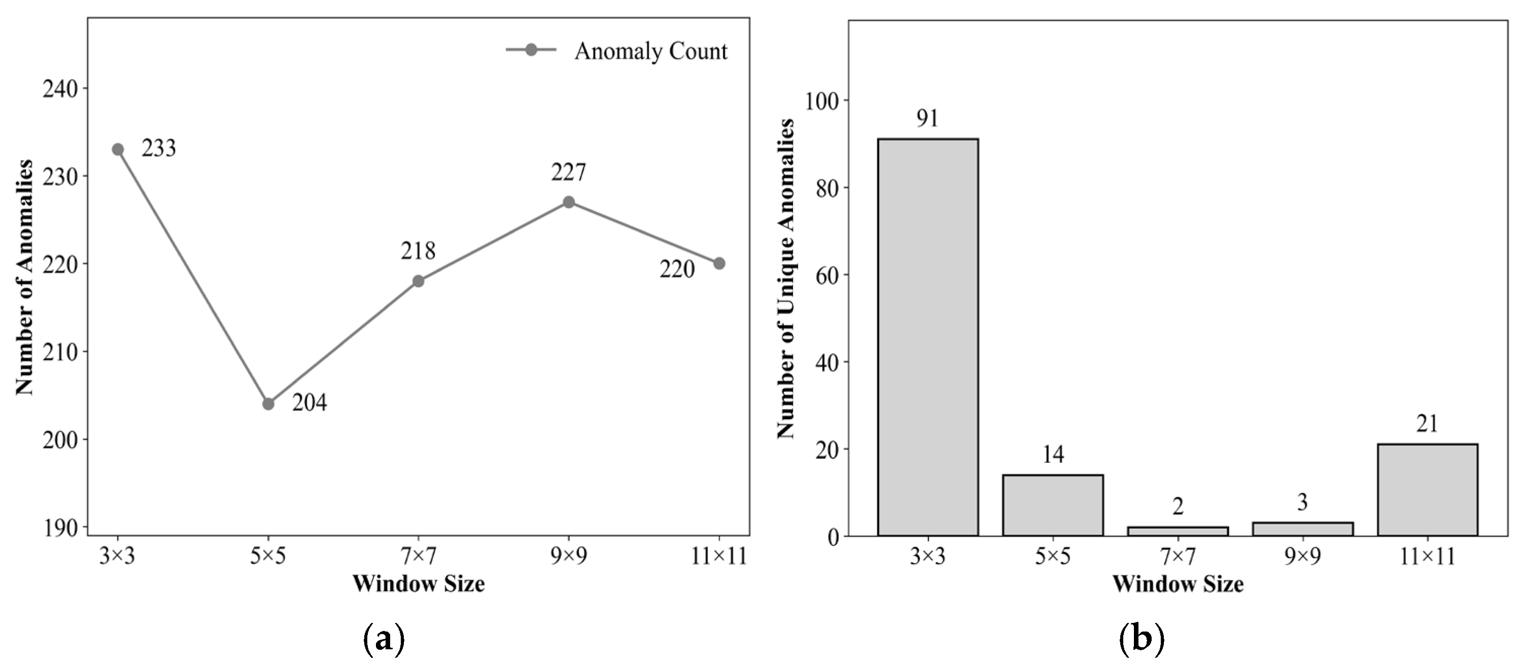
Appendix B.2.2. Overall Performance Comparison on the Full Dataset (Complete Two-Stage Framework)
Extending the window size sensitivity analysis to all data from the seven stations over 2016–2021, with k = 2 and the spatial anomaly threshold fixed, the complete two-stage detection framework was implemented. The overall average improvement rates and improvement ratios for each window size were calculated, and the total number of spatiotemporal anomaly points for each window was statistically analyzed.
Table A15 and Table A16 summarize the overall correction performance under different window sizes. It can be observed that: the 7 × 7 window achieves either the highest overall average improvement rates or values very close to the optimum for RMSE, MAE, and R (compared to the 9 × 9 window, the overall average improvement rate for RMSE is only 0.65 percentage points lower, and for MAE it is 0.37 percentage points lower). The overall average improvement rate for R2 is slightly lower than that of larger windows, yet its improvement ratio is on par with the 9 × 9 and 11 × 11 windows. The improvement ratios of the 7 × 7 window (RMSE 91.23%, MAE 91.23%, R 87.83%, R2 91.23%) are significantly higher than those of the 3 × 3 and 5 × 5 windows, while being comparable to those of the 9 × 9 and 11 × 11 windows. In terms of the number of detected anomaly points, the 7 × 7 window (1175) falls between the 5 × 5 (1367) and 9 × 9 (1128) windows, achieving the favorable balance between detection recall rate and correction reliability.
Table A15.
Overall average improvement rates and anomaly detection counts under different window sizes (k = 2, , 2016–2021).
Table A16.
Improvement proportions under different window sizes (%, 2016–2021).
Appendix B.2.3. Stability Analysis Across Different Seasons
To examine the performance differences in various window sizes under different seasonal climatic conditions and to evaluate the stability of the selected 7 × 7 window across the four seasons, this study further stratified the data by season and calculated the overall average improvement rates and improvement ratios for each window size in each season (Table A17, Table A18, Table A19 and Table A20).
In terms of the overall average improvement rate for RMSE (Table A17), the 7 × 7 window remains stable between 22% and 26% across all four seasons, with relatively small gaps compared to the 9 × 9 and 11 × 11 windows. Regarding the overall average improvement rate for MAE (Table A18), the performance difference between the 7 × 7 window and the 9 × 9 window in each season is within one percentage point, and it is also very close to that of the 11 × 11 window. For the overall average improvement rate of R (Table A19), except for winter, where the 7 × 7 window significantly outperforms larger windows, its performance in the remaining seasons is generally comparable to that of the 9 × 9 and 11 × 11 windows. The overall average improvement rate for R2 (Table A20) is on par with the 9 × 9 window in autumn but slightly lower than larger windows in the other seasons.
In terms of improvement ratios, the 7 × 7 window remains stable across the four seasons within the ranges of 89–94% (RMSE), 88–94% (MAE), 85–91% (R), and 89–94% (R2). These values are at the same level as those of the 9 × 9 and 11 × 11 windows, significantly higher than those of the 3 × 3 window, and show mixed results compared to the 5 × 5 window—either at a comparable level or slightly better.
The above results indicate that there is a clear “performance saturation zone” around the window size of 7 × 7: further increasing the window size yields very limited improvement in correction performance. Meanwhile, the 7 × 7 window achieves an optimal balance among computational efficiency, detection recall rate, and correction reliability, and remains unaffected by seasonal climatic conditions, demonstrating good cross-season stability.
Table A17.
Seasonal RMSE improvement rates and improvement proportions under different window sizes (%, k = 2, , 2016–2021).
Table A18.
Seasonal MAE improvement rates and improvement proportions under different window sizes (%, k = 2, , 2016–2021).
Table A19.
Seasonal R improvement rates and improvement proportions under different window sizes (%, k = 2, , 2016–2021).
Table A20.
Seasonal R2 improvement rates and improvement proportions under different window sizes (%, k = 2, , 2016–2021).
Appendix B.2.4. Stability Analysis Across Different Land Cover Types
To evaluate the stability of the spatial consistency check window size under different land surface types, this study classified the seven ground stations in the Heihe River Basin into four categories based on the underlying surface attributes in Table 2: alpine meadow (S1, S3), farmland/artificial vegetation (S2, S4), desert shrubland (S5, S6), and wetland (S7). With the temporal dimension threshold coefficient fixed at k = 2 and the spatial anomaly threshold fixed, the complete two-stage anomaly detection and IDW correction process was implemented using five window sizes: 3 × 3, 5 × 5, 7 × 7, 9 × 9, and 11 × 11. The overall average improvement rates and improvement ratios for each window size were calculated.
In terms of the overall average improvement rate for RMSE (Table A21), the 7 × 7 window achieves relatively high improvement magnitudes across all land cover types: alpine meadow (23.99%), farmland/artificial vegetation (23.46%), desert shrubland (24.21%), and wetland (22.29%). The differences between the 7 × 7 window and the 9 × 9 and 11 × 11 windows range from 0.21 to 1.64 percentage points, while it significantly outperforms the 3 × 3 and 5 × 5 windows. Regarding the improvement ratio for RMSE, the 7 × 7 window exhibits excellent performance across all land cover types, reaching its highest value in desert shrubland (94.86%), demonstrating good correction reliability.
In terms of MAE, R, and R2 metrics (Table A22, Table A23 and Table A24), the 7 × 7 window performs well across all land cover types. For the overall average improvement rate of MAE, the differences between the 7 × 7 window and the 9 × 9 and 11 × 11 windows are relatively small, and it significantly outperforms the 3 × 3 and 5 × 5 windows. Regarding the overall average improvement rate of R, except for farmland/artificial vegetation, where the 7 × 7 window (23.36%) is significantly higher than the 9 × 9 (13.17%) and 11 × 11 (9.59%) windows, the 7 × 7 window is generally comparable to larger windows in other land cover types. For the overall average improvement rate of R2, the 7 × 7 window is lower than the 9 × 9 and 11 × 11 windows in most land cover types but outperforms the 3 × 3 and 5 × 5 windows; in farmland/artificial vegetation, although the 7 × 7 window (59.04%) is lower than the 5 × 5 window (99.53%), it remains significantly better than the 3 × 3 window (39.56%). In terms of improvement ratios, the 7 × 7 window is close to the 9 × 9 and 11 × 11 windows across all metrics and land cover types, and significantly outperforms the 3 × 3 and 5 × 5 windows.
From the perspective of cross-land cover stability, the performance of the 7 × 7 window exhibits minimal fluctuation across different land cover types, closely aligning with the overall average levels of the Heihe River Basin. The above results indicate that the 7 × 7 window consistently achieves a favorable balance between correction magnitude and correction reliability under different surface thermal backgrounds. Further increasing the window size yields very limited performance improvement, while the 7 × 7 window achieves a favorable trade-off among computational efficiency, correction magnitude, and correction reliability.
Table A21.
RMSE improvement rates and improvement proportions under different window sizes and land cover types (%, k = 2, , 2016–2021).
Table A22.
MAE improvement rates and improvement proportions under different window sizes and land cover types (%, k = 2, , 2016–2021).
Table A23.
R improvement rates and improvement proportions under different window sizes and land cover types (%, k = 2, , 2016–2021).
Table A24.
R2 improvement rates and improvement proportions under different window sizes and land cover types (%, k = 2, , 2016–2021).
Appendix B.3. Sensitivity Analysis of the Spatial Anomaly Threshold
Appendix B.3.1. Overall Performance Comparison on the Full Dataset (Complete Two-Stage Framework)
Extending the spatial anomaly threshold sensitivity analysis to all data from the seven stations over 2016–2021, with k = 2 and the 7 × 7 window fixed, the complete two-stage detection framework was implemented. The overall average improvement rates and improvement ratios were calculated for threshold settings of 2.0, 2.5, 3.0, and 3.5, and the total number of spatiotemporal anomaly points under each threshold was statistically analyzed.
Table A25 and Table A26 summarize the overall correction performance under different thresholds. It can be observed that: a threshold achieves the highest overall average improvement rate for R (16.46%), while its overall average improvement rates for RMSE and MAE are slightly lower than those of , with gaps of 0.95 and 0.66 percentage points, respectively. The overall average improvement rate for R2 under 3.0 is 4.15 percentage points lower than that under . Its improvement ratios are slightly lower than those of , with all gaps within 1.3 percentage points (RMSE difference 1.26, MAE difference 1.05, R difference 0.65, R2 difference 1.26 percentage points), while being significantly higher than those under and .
In terms of the number of detected anomaly points, the threshold detects the largest number (1858), but its overall average improvement rates and improvement ratios are the lowest, indicating that numerous spatially consistent normal fluctuations are misjudged as anomalies. The threshold detects the fewest anomaly points (1046), with slightly higher overall average improvement rates; however, its improvement ratios are generally comparable to those of , and the risk of missed detection increases. The threshold achieves a good balance between detection recall rate (1175 points) and correction reliability, indicating good comprehensive performance.
Table A25.
Overall average improvement rates and anomaly detection counts under different thresholds (k = 2, 7 × 7 window, 2016–2021).
Table A26.
Improvement proportions under different thresholds (%, k = 2, 7 × 7 window, 2016–2021).
Appendix B.3.2. Stability Analysis Across Different Seasons
To examine the performance differences in various thresholds under different seasonal climatic conditions and to evaluate the stability of the selected threshold across the four seasons, this study further stratified the data by season. With k = 2 and the 7 × 7 window fixed, the overall average improvement rates and improvement ratios for each metric under each threshold were calculated for each season (Table A27, Table A28, Table A29 and Table A30).
Table A27, Table A28, Table A29 and Table A30 systematically present the seasonal decomposition comparison of the four core evaluation metrics under different thresholds . In terms of overall average improvement rates, the performance of across seasons is generally consistent with the overall results of . For RMSE and MAE, achieves slightly higher overall average improvement rates than , with differences within 2 percentage points. For the overall average improvement rate of R, significantly outperforms in winter (28.42% vs. 20.08%), demonstrating better effectiveness. Regarding the overall average improvement rate of R2, is slightly higher than in all seasons, with relatively larger gaps in autumn and winter (5.61 and 6.18 percentage points, respectively), while , still maintaining a relatively high improvement magnitude. Both and are significantly better than and generally outperforms overall.
In terms of improvement ratios, the fluctuation ranges of across seasons are 89–94% for RMSE, 88–94% for MAE, 85–91% for R, and 89–94% for R2, which are at the same level as . Compared to , is slightly better or comparable in spring, summer, and winter, while is slightly lower in autumn, though the differences are minimal. The improvement ratios of both and are significantly higher than those of .
From the perspective of cross-season stability, the performance of exhibits minimal fluctuation across seasons, closely aligning with the overall average levels. Considering the number of detected anomaly points ( detects 1175 points, falling between the 1858 points of and the 1,046 points of ), achieves a favorable balance between correction magnitude and correction reliability, remains unaffected by seasonal climatic conditions, and demonstrates good cross-scenario stability.
Table A27.
Seasonal RMSE improvement rates and improvement proportions under different thresholds (k = 2, 7 × 7 window, 2016–2021).
Table A28.
Seasonal MAE improvement rates and improvement proportions under different thresholds (k = 2, 7 × 7 window, 2016–2021).
Table A29.
Seasonal R improvement rates and improvement proportions under different thresholds (k = 2, 7 × 7 window, 2016–2021).
Table A30.
Seasonal R2 improvement rates and improvement proportions under different thresholds (k = 2, 7 × 7 window, 2016–2021).
Appendix B.3.3. Stability Analysis Across Different Land Cover Types
To evaluate the stability of the selected spatial anomaly threshold under different land surface types, this study classified the seven ground stations in the Heihe River Basin into four categories based on underlying surface attributes: alpine meadow (S1, S3), farmland/artificial vegetation (S2, S4), desert shrubland (S5, S6), and wetland (S7). The hourly LST data from all stations within each category for 2016–2021 were aggregated. With the temporal dimension threshold coefficient fixed at k = 2 and the spatial consistency check window size fixed at 7 × 7, the complete two-stage anomaly detection and IDW correction process was implemented under four threshold settings (2.0, 2.5, 3.0, and 3.5).
Table A31, Table A32, Table A33 and Table A34 present the overall average improvement rates and improvement ratios for various metrics across the four land cover types under different thresholds . In terms of overall average improvement rates, is slightly higher than in most cases, but the differences are generally small. Specifically, for RMSE, is slightly higher across all land cover types, with gaps of 1.12, 1.12, 0.02, and 1.69 percentage points in alpine meadow, farmland/artificial vegetation, desert shrubland, and wetland, respectively, with the desert shrubland gap being nearly negligible. For MAE, except in desert shrubland, where slightly surpasses by 0.05 percentage points, outperforms by 0.63 to 1.17 percentage points in the other land cover types. For the R metric, (23.36%) is significantly higher than (15.36%) in farmland/artificial vegetation, while in other land cover types, is slightly higher with gaps all below 2.4 percentage points. For R2, exceeds by approximately 1.48 and 1.93 percentage points in farmland/artificial vegetation and desert shrubland, respectively, with even larger gaps of in wetland and alpine meadow—15.05 and 5.11 percentage points, respectively. Overall, the performance of and is very close, and both significantly outperform and , whose improvement magnitudes and ratios are notably lower.
In terms of improvement ratios, remains highly consistent with . For example, the difference in RMSE improvement ratios between the two thresholds ranges from 0.27 to 2.15 percentage points, and the difference in MAE improvement ratios ranges from 0.27 to 2.11 percentage points. For the R metric, the improvement ratio of in desert shrubland (91.78%) is even higher than that of (91.15%), while differences in other land cover types are all within 1.79 percentage points. The differences in R2 improvement ratios also do not exceed 2.15 percentage points. This indicates that is essentially comparable to in terms of correction reliability.
From the perspective of cross-land cover stability, the performance of exhibits minimal fluctuation across different land cover types, closely aligning with the overall average levels of the Heihe River Basin. Considering the number of detected anomaly points ( detects 1,175 points, falling between the 1858 points of and the 1046 points of ), while maintaining correction performance similar to , detects more anomaly points, has a significantly lower risk of missed detection than , and a much lower risk of false detection than . Therefore, achieves a favorable balance between correction magnitude and correction reliability across different land surface types, indicating good robustness.
Table A31.
RMSE improvement rates and improvement proportions under different || thresholds and land cover types (k = 2, 7 × 7 window, 2016–2021).
Table A32.
MAE improvement rates and improvement proportions under different || thresholds and land cover types (k = 2, 7 × 7 window, 2016–2021).
Table A33.
R improvement rates and improvement proportions under different || thresholds and land cover types (k = 2, 7 × 7 window, 2016–2021).
Table A34.
R2 improvement rates and improvement proportions under different || thresholds and land cover types (k = 2, 7 × 7 window, 2016–2021).
Appendix C
This appendix provides a detailed explanation of the principles underlying the comparative methods discussed in Section 4.5 of the main text, along with comprehensive correction performance data, including the recursive equations and parameter settings of the robust Holt–Winters method, the year-by-year correction results, and a comparative analysis with the method proposed in this paper.
To further compare with robust filtering methods, this study introduces the robust Holt–Winters filtering approach proposed by Gelper et al. This method effectively mitigates the impact of anomalies on trend and seasonal components by recursively updating and cleaning observations in real time, representing a typical online robust filtering technique. Its core recursive equations are as follows:
where is the Huber function, with its threshold set to the commonly used value recommended by Gelper et al.; is the recursive estimate of the residual scale (estimated using the biweight estimator , with the smoothing parameter also determined based on the simulation settings in the literature). The seasonal period is determined according to the diurnal variation characteristics of land surface temperature data. The smoothing parameters are adaptively determined by minimizing the scale via grid search, with their value ranges set to [0.2, 0.8], [0.1, 0.4], and [0.1, 0.4], respectively, and a step size of 0.1. These ranges refer to the common intervals for classical Holt–Winters smoothing parameters. After filtering, moments where the absolute value of the standardized residual exceeds the threshold of 3 are flagged as anomalies, and the cleaned value is used as the corrected value for that moment.
Table A35, Table A36 and Table A37 present the annual and average correction performance of this method from 2016 to 2021.
As shown in Table A37, the robust Holt–Winters method improves approximately 60% of the anomaly points in terms of RMSE, MAE, R, and R2; however, its overall average improvement rate remains relatively low. Table A35 indicates that the six-year overall average improvement rates for RMSE and MAE are only 1.66% and 0.94%, respectively, while Table A36 shows that the overall average improvement rates for R and R2 are merely 0.53% and 0.94%. These results suggest that although this method can identify a certain proportion of anomalies, its reliance solely on temporal information—lacking spatial contextual constraints—leads to very limited correction magnitudes and a relatively high false detection rate (with an annual average of 2258 detected anomalies, far exceeding the 195.83 detected by the method proposed in this paper).
Compared with the two-stage anomaly detection framework proposed in this paper, the method presented herein shows advantages across all metrics. First, in terms of anomaly identification, the proposed method, through temporal preliminary screening and spatial verification, detects an annual average of only 195.83 anomaly points—far fewer than the robust Holt–Winters method—indicating a lower false detection rate and higher targeting precision. Second, regarding correction effectiveness, the improvement ratios of RMSE and MAE achieved by the proposed method reach as high as 91.23% and 91.23%, respectively, outperforming the approximately 60% achieved by robust Holt–Winters. In terms of overall average improvement rates, the proposed method attains 23.61% for RMSE and 18.79% for MAE, as well as 16.46% for R and 61.33% for R2, whereas all overall average improvement rates of robust Holt–Winters are below 2%. This demonstrates that, through its two-stage design incorporating temporal Pre-Screening and spatial verification, the proposed method can more accurately locate genuine anomaly points and effectively correct them by leveraging spatial neighborhood information, thereby significantly enhancing correction accuracy and stability.
In summary, although the robust Holt–Winters method can identify some anomaly points, its reliance solely on temporal information—lacking spatial contextual constraints—leads to limited correction magnitudes and a relatively high false detection rate. As shown in the comprehensive comparison in Section 4.5, the proposed method outperforms existing comparative methods—including robust Holt–Winters—in terms of detection accuracy, correction magnitude, and stability.
Table A35.
Comparison of error metrics and overall average improvement rates before and after Robust Holt–Winters correction (2016–2021).
Table A36.
Comparison of correlation metrics and overall average improvement rates before and after Robust Holt–Winters correction (2016–2021).
Table A37.
Improvement proportion of Robust Holt–Winters method (%, 2016–2021).
References
- Wang, Y.; Li, J.; Sun, H.; Li, X. A review on the developments and space applications of mid- and long-wavelength infrared detection technologies. Front. Inf. Technol. Electron. Eng. 2024, 25, 1031–1057. [Google Scholar] [CrossRef] [Scilit]
- Sobrino, J.A.; Frate, F.D.; Drusch, M.; Jiménez-Muñoz, J.C.; Manunta, P.; Regan, A. Review of Thermal Infrared Applications and Requirements for Future High-Resolution Sensors. IEEE Trans. Geosci. Remote Sens. 2016, 54, 2963–2972. [Google Scholar] [CrossRef] [Scilit]
- Xia, H. Geographically Constrained Machine Learning-Based Kernel-Driven Method for Downscaling of All-Weather Land Surface Temperature. Remote Sens. 2025, 17, 1413. [Google Scholar] [CrossRef] [Scilit]
- Mishra, A.; Ohri, A.; Singh, P.K.; Singh, N.; Calay, R.K. Improving the Prediction of Land Surface Temperature Using Hyperparameter-Tuned Machine Learning Algorithms. Atmosphere 2025, 16, 1295. [Google Scholar] [CrossRef] [Scilit]
- Wang, J.; Li, C. Development and prospect of hyperspectral imager and its application. Chin. J. Space 2021, 41, 22–33. (In Chinese) [Google Scholar] [CrossRef] [Scilit]
- Riba, A.; Garcia, M.; Tarquís, A.M.; Domingo, F.; Antala, M.; Feng, S.; Liu, J.; Johnson, M.S.; Kim, Y.; Wang, S. Integrating Remotely Sensed Thermal Observations for Calibration of Process-Based Land-Surface Models: Accuracy, Revisit Windows, and Implications in a Dryland Ecosystem. Remote Sens. 2025, 17, 3630. [Google Scholar]
- Wu, H.; Li, X.J.; Li, Z.L.; Duan, S.B.; Qian, Y.G. Hyperspectral thermal infrared remote sensing: Current status and perspectives. Natl. Remote Sens. Bull. 2021, 25, 1567–1590. [Google Scholar] [CrossRef] [Scilit]
- Zhou, D.; Xiao, J.; Bonafoni, S.; Berger, C.; Deilami, K.; Zhou, Y.; Frolking, S.; Yao, R.; Qiao, Z.; Sobrino, J.A. Satellite Remote Sensing of Surface Urban Heat Islands: Progress, Challenges, and Perspectives. Remote Sens. 2018, 11, 48. [Google Scholar] [CrossRef] [Scilit]
- Anderson, M.C.; Kustas, W.P.; Norman, J.M.; Hain, C.R.; Mecikalski, J.R.; Schultz, L.; González-Dugo, M.P.; Cammalleri, C.; D’Urso, G.; Pimstein, A.; et al. Mapping daily evapotranspiration at field to continental scales using geostationary and polar orbiting satellite imagery. Hydrol. Earth Syst. Sci. 2011, 15, 223–239. [Google Scholar] [CrossRef] [Scilit]
- Li, X.; Xiao, J.; Fisher, J.B.; Baldocchi, D.D. ECOSTRESS estimates gross primary production with fine spatial resolution for different times of day from the International Space Station. Remote Sens. Environ. 2021, 258, 112360. [Google Scholar] [CrossRef] [Scilit]
- Tang, Y.; Zhao, Y.; Sun, Y.; Ren, S.; Li, Z. Seamless Reconstruction of MODIS Land Surface Temperature via Multi-Source Data Fusion and Multi-Stage Optimization. Remote Sens. 2025, 17, 3374. [Google Scholar] [CrossRef] [Scilit]
- Mo, Y.; Xu, Y.; Chen, H.; Zhu, S. A Review of Reconstructing Remotely Sensed Land Surface Temperature under Cloudy Conditions. Remote Sens. 2021, 13, 2838. [Google Scholar] [CrossRef] [Scilit]
- Tan, W.; Wei, C.; Lu, Y.; Xue, D. Reconstruction of All-Weather Daytime and Nighttime MODIS Aqua-Terra Land Surface Temperature Products Using an XGBoost Approach. Remote Sens. 2021, 13, 4723. [Google Scholar] [CrossRef] [Scilit]
- Zhang, Y.; Chen, Y.; Li, J.; Chen, X. A Simple Method for Converting 1-km Resolution Daily Clear-Sky LST into Real LST. Remote Sens. 2020, 12, 1641. [Google Scholar] [CrossRef] [Scilit]
- Jia, A. Estimation and Spatiotemporal Analysis of All-Sky Land Surface Temperature from Multiple Satellite Data. Ph.D. Thesis, University of Maryland, College Park, MD, USA, 2023. [Google Scholar]
- Wu, P.; Yin, Z.; Zeng, C.; Duan, S.-B.; Gottsche, F.-M.; Ma, X.; Li, X.; Yang, H.; Shen, H. Spatially Continuous and High-Resolution Land Surface Temperature Product Generation: A review of reconstruction and spatiotemporal fusion techniques. IEEE Geosci. Remote Sens. Mag. 2021, 9, 112–137. [Google Scholar] [CrossRef] [Scilit]
- Xu, S.; Cheng, J.; Zhang, Q. A Random Forest-Based Data Fusion Method for Obtaining All-Weather Land Surface Temperature with High Spatial Resolution. Remote Sens. 2021, 13, 2211. [Google Scholar] [CrossRef] [Scilit]
- Duan, S.-B.; Han, X.-J.; Huang, C.; Li, Z.-L.; Wu, H.; Qian, Y.; Gao, M.; Leng, P. Land Surface Temperature Retrieval from Passive Microwave Satellite Observations: State-of-the-Art and Future Directions. Remote Sens. 2020, 12, 2573. [Google Scholar] [CrossRef] [Scilit]
- Xu, S.; Cheng, J. A new land surface temperature fusion strategy based on cumulative distribution function matching and multiresolution Kalman filtering. Remote Sens. Environ. 2021, 254, 112256. [Google Scholar] [CrossRef] [Scilit]
- Zhong, Y.; Meng, L.; Wei, Z.; Yang, J.; Song, W.; Basir, M. Retrieval of All-Weather 1 km Land Surface Temperature from Combined MODIS and AMSR2 Data over the Tibetan Plateau. Remote Sens. 2021, 13, 4574. [Google Scholar] [CrossRef] [Scilit]
- Li, Y.; Zhu, S.; Luo, Y.; Zhang, G.; Xu, Y. Reconstruction of Land Surface Temperature Derived from FY-4A AGRI Data Based on Two-Point Machine Learning Method. Remote Sens. 2023, 15, 5179. [Google Scholar] [CrossRef] [Scilit]
- Trigo, I.F.; Boussetta, S.; Viterbo, P.; Balsamo, G.; Beljaars, A.; Sandu, I. Comparison of model land skin temperature with remotely sensed estimates and assessment of surface-atmosphere coupling. J. Geophys. Res. Atmos. 2015, 120, 12096–12111. [Google Scholar] [CrossRef] [Scilit]
- Dong, S.; Cheng, J.; Shi, J.; Shi, C.; Sun, S.; Liu, W. A Data Fusion Method for Generating Hourly Seamless Land Surface Temperature from Himawari-8 AHI Data. Remote Sens. 2022, 14, 5170. [Google Scholar] [CrossRef] [Scilit]
- Holmes, T.R.H.; Crow, W.T.; Hain, C. Spatial patterns in timing of the diurnal temperature cycle. Hydrol. Earth Syst. Sci. 2013, 17, 3695–3706. [Google Scholar] [CrossRef] [Scilit]
- Kwok, C.F.; Qian, G.Q.; Kuleshov, Y. Analyzing Error Bounds for Seasonal-Trend Decomposition of Antarctica Temperature Time Series Involving Missing Data. Atmosphere 2023, 14, 193. [Google Scholar] [CrossRef] [Scilit]
- Dash, P.; Saha, K.; DiGiacomo, P.; Miller, S.D.; Zhang, H.M.; Lazzaro, R.; Son, S. Trends in Satellite-Based Ocean Parameters through Integrated Time Series Decomposition and Spectral Analysis. Part I: Chlorophyll, Sea Surface Temperature, and Sea Level Anomaly. J. Atmos. Ocean. Technol. 2025, 42, 91–123. [Google Scholar] [CrossRef] [Scilit]
- Benschop, N.D.; Zewotir, T.; Naidoo, R.N.; North, D. A new data-standardization procedure for comprehensive outlier detection in correlated meteorological sensor data. Adv. Stat. Clim. Meteorol. Oceanogr. 2025, 11, 133–158. [Google Scholar] [CrossRef] [Scilit]
- Kim, H.-J.; Park, S.M.; Choi, B.J.; Moon, S.-H.; Kim, Y.-H. Spatiotemporal Approaches for Quality Control and Error Correction of Atmospheric Data through Machine Learning. Comput. Intell. Neurosci. 2020, 2020, 7980434. [Google Scholar] [CrossRef] [Scilit]
- Xie, C.J.; Huang, C.; Zhang, D.Q.; He, W. BiLSTM-I: A Deep Learning-Based Long Interval Gap-Filling Method for Meteorological Observation Data. Int. J. Environ. Res. Public Health 2021, 18, 321. [Google Scholar] [CrossRef] [Scilit] [PubMed]
- Faybishenko, B.; Versteeg, R.; Pastorello, G.; Dwivedi, D.; Varadharajan, C.; Agarwal, D. Challenging problems of quality assurance and quality control (QA/QC) of meteorological time series data. Stoch. Environ. Res. Risk Assess. 2022, 36, 1049–1062. [Google Scholar] [CrossRef] [Scilit]
- Cheng, A.R.; Lee, T.H.; Ku, H.I.; Chen, Y.W. Quality Control Program for Real-Time Hourly Temperature Observation in Taiwan. J. Atmos. Ocean. Technol. 2016, 33, 953–976. [Google Scholar] [CrossRef] [Scilit]
- Collins, G.Q.; Heaton, M.J.; Hu, L.Q. Physically constrained spatiotemporal modeling: Generating clear-sky constructions of land surface temperature from sparse, remotely sensed satellite data. J. Appl. Stat. 2020, 47, 1439–1459. [Google Scholar] [CrossRef] [Scilit] [PubMed]
- Zhou, S.; Cheng, J. An Improved Temperature and Emissivity Separation Algorithm for the Advanced Himawari Imager. IEEE Trans. Geosci. Remote Sens. 2020, 58, 7105–7124. [Google Scholar] [CrossRef] [Scilit]
- Cheng, J.; Dong, S.; Shi, J. 0.02° Seamless Hourly Land Surface Temperature Dataset over East Asia (2016–2021); National Tibetan Plateau/Third Pole Environment Data Center: Beijing, China, 2022. [Google Scholar] [CrossRef]
- Xu, Z.W.; Liu, S.M.; Che, T. Operation and maintenance and data quality control of the Heihe integrated observatory network. Resour. Sci. 2020, 42, 1975–1986. [Google Scholar] [CrossRef] [Scilit]
- Che, T.; Li, X.; Liu, S.; Li, H.; Xu, Z.; Tan, J.; Zhang, Y.; Ren, Z.; Xiao, L.; Deng, J.; et al. Integrated hydrometeorological, snow and frozen-ground observations in the alpine region of the Heihe River Basin, China. Earth Syst. Sci. Data 2019, 11, 1483–1499. [Google Scholar] [CrossRef] [Scilit]
- Liu, S.; Li, X.; Xu, Z.; Che, T.; Xiao, Q.; Ma, M.; Liu, Q.; Jin, R.; Guo, J.; Wang, L.; et al. The Heihe Integrated Observatory Network: A Basin-Scale Land Surface Processes Observatory in China. Vadose Zone J. 2018, 17, 1–21. [Google Scholar] [CrossRef] [Scilit]
- Liang, S.; Cheng, J.; Jia, K.; Jiang, B.; Liu, Q.; Xiao, Z.; Yao, Y.; Yuan, W.; Zhang, X.; Zhao, X.; et al. The Global Land Surface Satellite (GLASS) Product Suite. Bull. Am. Meteorol. Soc. 2021, 102, E323–E337. [Google Scholar] [CrossRef] [Scilit]
- Cheng, J.; Liang, S. Estimating the broadband longwave emissivity of global bare soil from the MODIS shortwave albedo product. J. Geophys. Res. Atmos. 2014, 119, 614–634. [Google Scholar] [CrossRef] [Scilit]
- Cheng, J.; Liang, S.; Verhoef, W.; Shi, L.; Liu, Q. Estimating the Hemispherical Broadband Longwave Emissivity of Global Vegetated Surfaces Using a Radiative Transfer Model. IEEE Trans. Geosci. Remote Sens. 2016, 54, 905–917. [Google Scholar] [CrossRef] [Scilit]
- Liu, S.; Xu, Z. Multi-Scale Surface Flux and Meteorological Elements Observation Dataset in the Hai River Basin (Huailai Station-Automatic Weather Station-10 m Tower, 2021); National Tibetan Plateau/Third Pole Environment Data Center: Beijing, China, 2022. [Google Scholar] [CrossRef]
- Liu, S.M.; Xu, Z.W.; Zhu, Z.L.; Jia, Z.Z.; Zhu, M.J. Measurements of evapotranspiration from eddy-covariance systems and large aperture scintillometers in the Hai River Basin, China. J. Hydrol. 2013, 487, 24–38. [Google Scholar] [CrossRef] [Scilit]
- Guo, A.; Liu, S.; Zhu, Z.; Xu, Z.; Xiao, Q.; Ju, Q.; Zhang, Y.; Yang, X. Impact of Lake/Reservoir Expansion and Shrinkage on Energy and Water Vapor Fluxes in the Surrounding Area. J. Geophys. Res. Atmos. 2020, 125, e2020JD032833. [Google Scholar] [CrossRef] [Scilit]
- Wang, X.; Prigent, C. Comparisons of Diurnal Variations of Land Surface Temperatures from Numerical Weather Prediction Analyses, Infrared Satellite Estimates and In Situ Measurements. Remote Sens. 2020, 12, 583. [Google Scholar] [CrossRef] [Scilit]
- Sassi, M.Z.; Fourrié, N.; Guidard, V.; Birman, C. Use of Infrared Satellite Observations for the Surface Temperature Retrieval over Land in a NWP Context. Remote Sens. 2019, 11, 2371. [Google Scholar] [CrossRef] [Scilit]
- Chen, W.; Pinker, R.T.; Ma, Y.; Hulley, G.C.; Borbas, E.; Islam, T.; Cawse-Nicholson, K.A.; Hook, S.J.; Hain, C.R.; Basara, J.B. Land Surface Temperature from GOES-East and GOES-West. J. Atmos. Ocean. Technol. 2021, 38, 843–858. [Google Scholar] [CrossRef] [Scilit]
- Martin, M.A.; Ghent, D.; Pires, A.C.; Göttsche, F.-M.; Cermak, J.; Remedios, J.J. Comprehensive In Situ Validation of Five Satellite Land Surface Temperature Data Sets over Multiple Stations and Years. Remote Sens. 2019, 11, 479. [Google Scholar] [CrossRef] [Scilit]
- Pinker, R.T.; Ma, Y.; Chen, W.; Hulley, G.; Borbas, E.; Islam, T.; Hain, C.; Cawse-Nicholson, K.; Hook, S.; Basara, J. Towards a Unified and Coherent Land Surface Temperature Earth System Data Record from Geostationary Satellites. Remote Sens. 2019, 11, 1399. [Google Scholar] [CrossRef] [Scilit]
- Scarino, B.R.; Minnis, P.; Chee, T.; Bedka, K.M.; Yost, C.R.; Palikonda, R. Global clear-sky surface skin temperature from multiple satellites using a single-channel algorithm with angular anisotropy corrections. Atmos. Meas. Tech. 2017, 10, 351–371. [Google Scholar] [CrossRef] [Scilit]
- Fang, L.; Yu, Y.Y.; Xu, H.; Sun, D.L. New Retrieval Algorithm for Deriving Land Surface Temperature from Geostationary Orbiting Satellite Observations. IEEE Trans. Geosci. Remote Sens. 2014, 52, 819–828. [Google Scholar] [CrossRef]
- Göttsche, F.-M.; Olesen, F.S. Modeling of diurnal cycles of brightness temperature extracted from METEOSAT data. Remote Sens Environ. Remote Sens. Environ. 2001, 76, 337–348. [Google Scholar] [CrossRef] [Scilit]
- Burrough, P.A.; McDonnell, R.A.; Lloyd, C.D. Principles of Geographical Information Systems, 3rd ed.; Oxford University Press: Oxford, UK, 2015. [Google Scholar]
- Cleveland, R.B.; Cleveland, W.S. STL: A seasonal-trend decomposition procedure based on Loess. J. Off. Stat. 1990, 6, 3–73. [Google Scholar]
- Gelper, S.; Fried, R.; Croux, C. Robust forecasting with exponential and Holt–Winters smoothing. J. Forecast. 2010, 29, 285–300. [Google Scholar] [CrossRef] [Scilit]
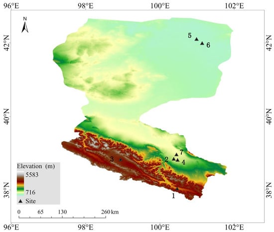
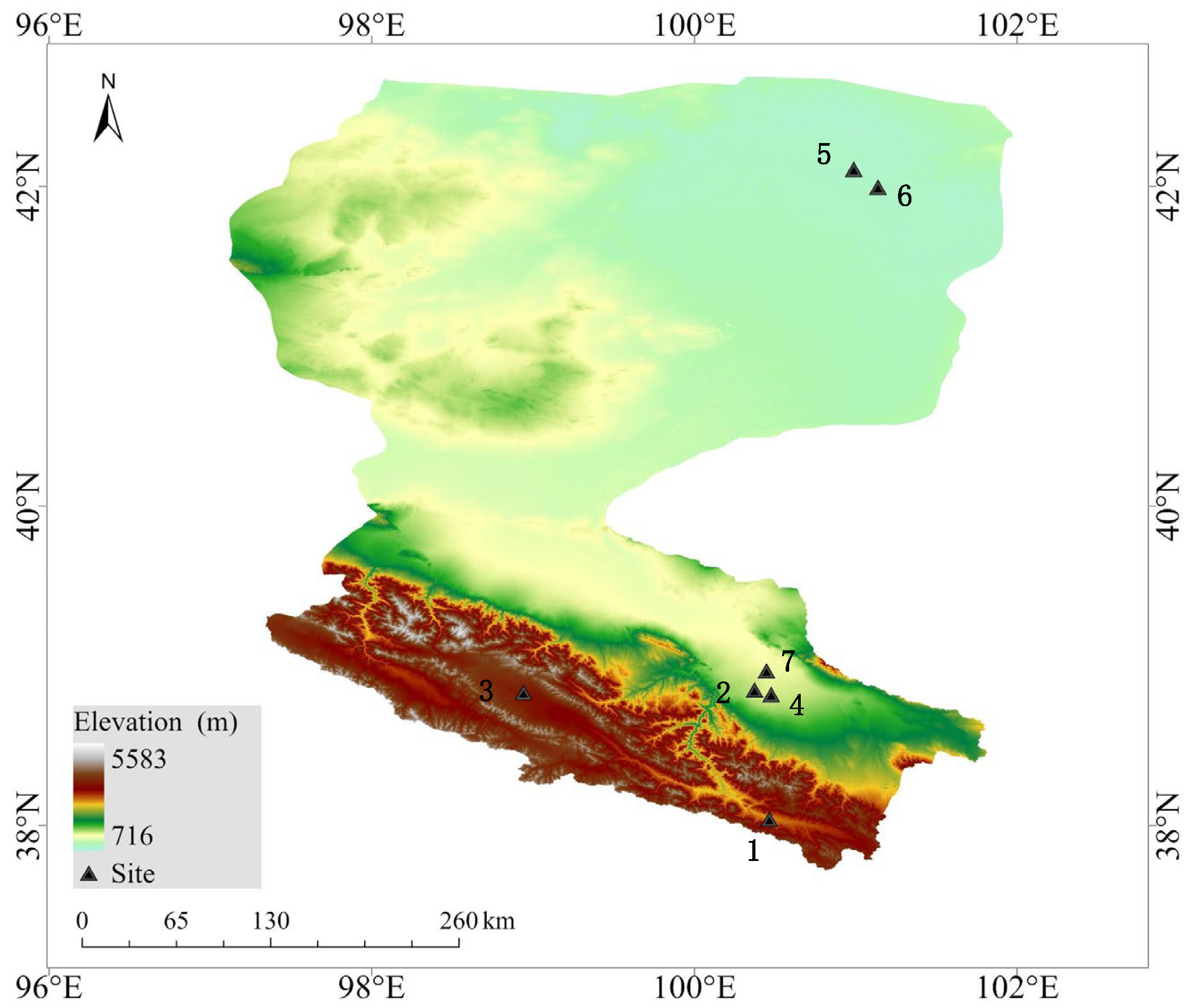
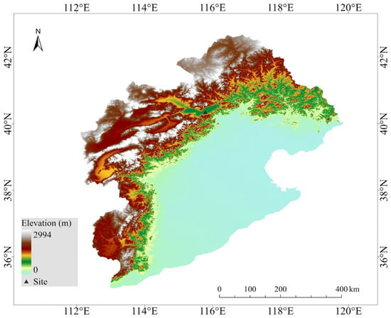
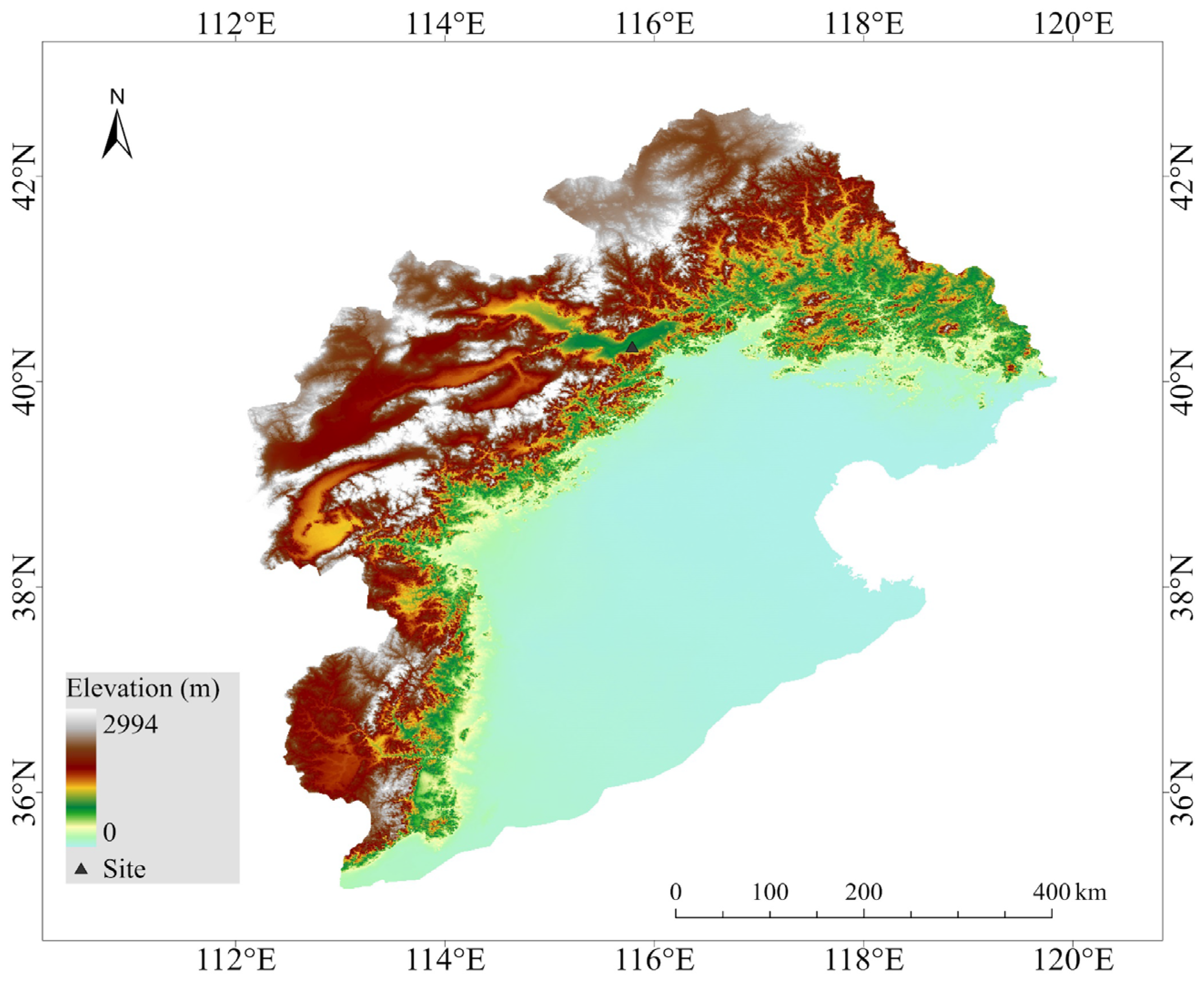
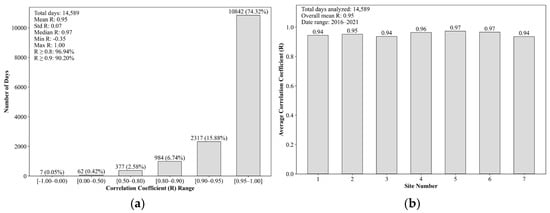
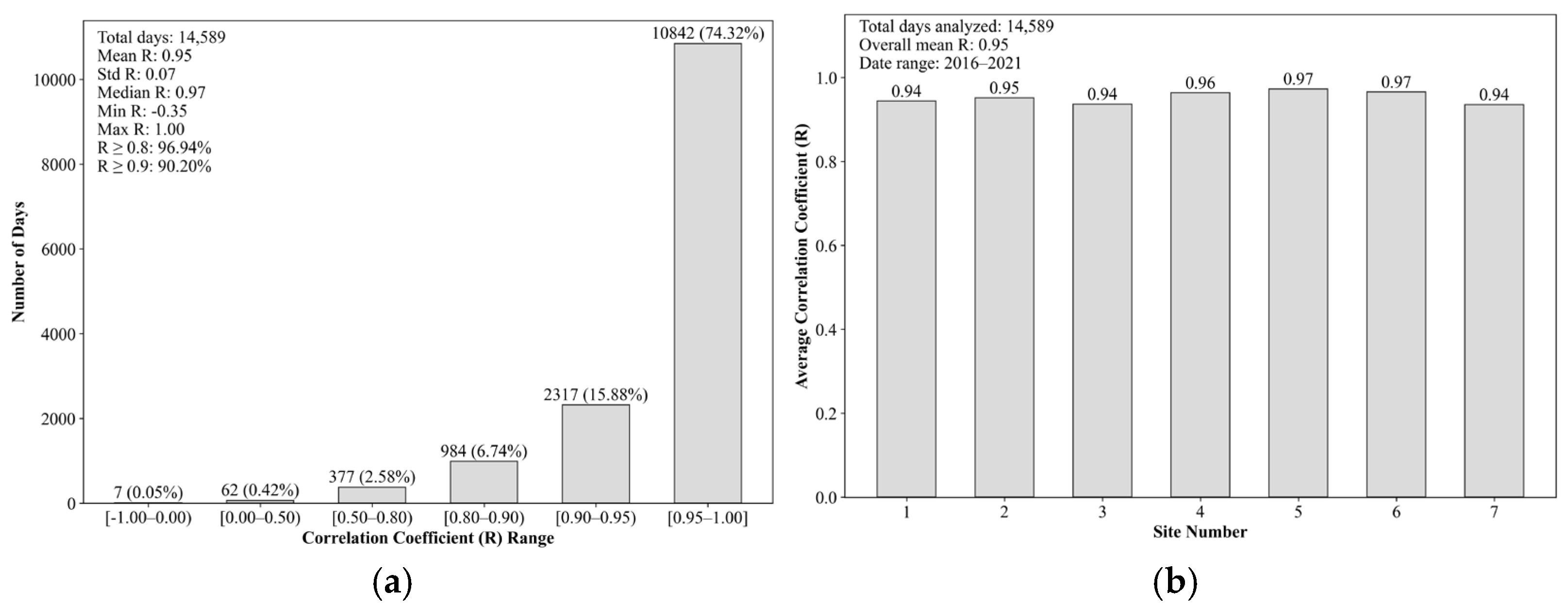
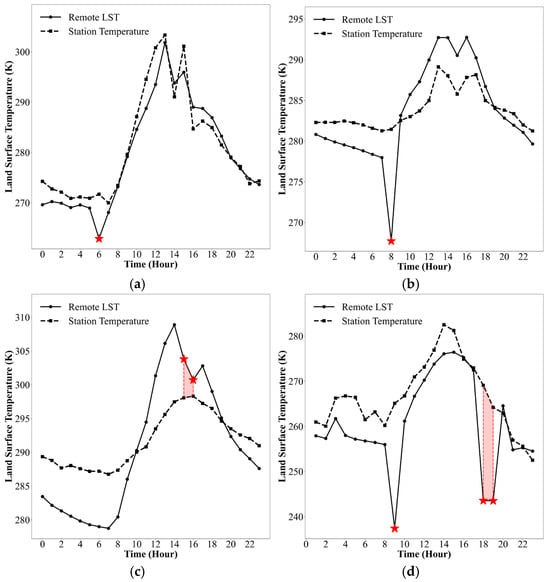
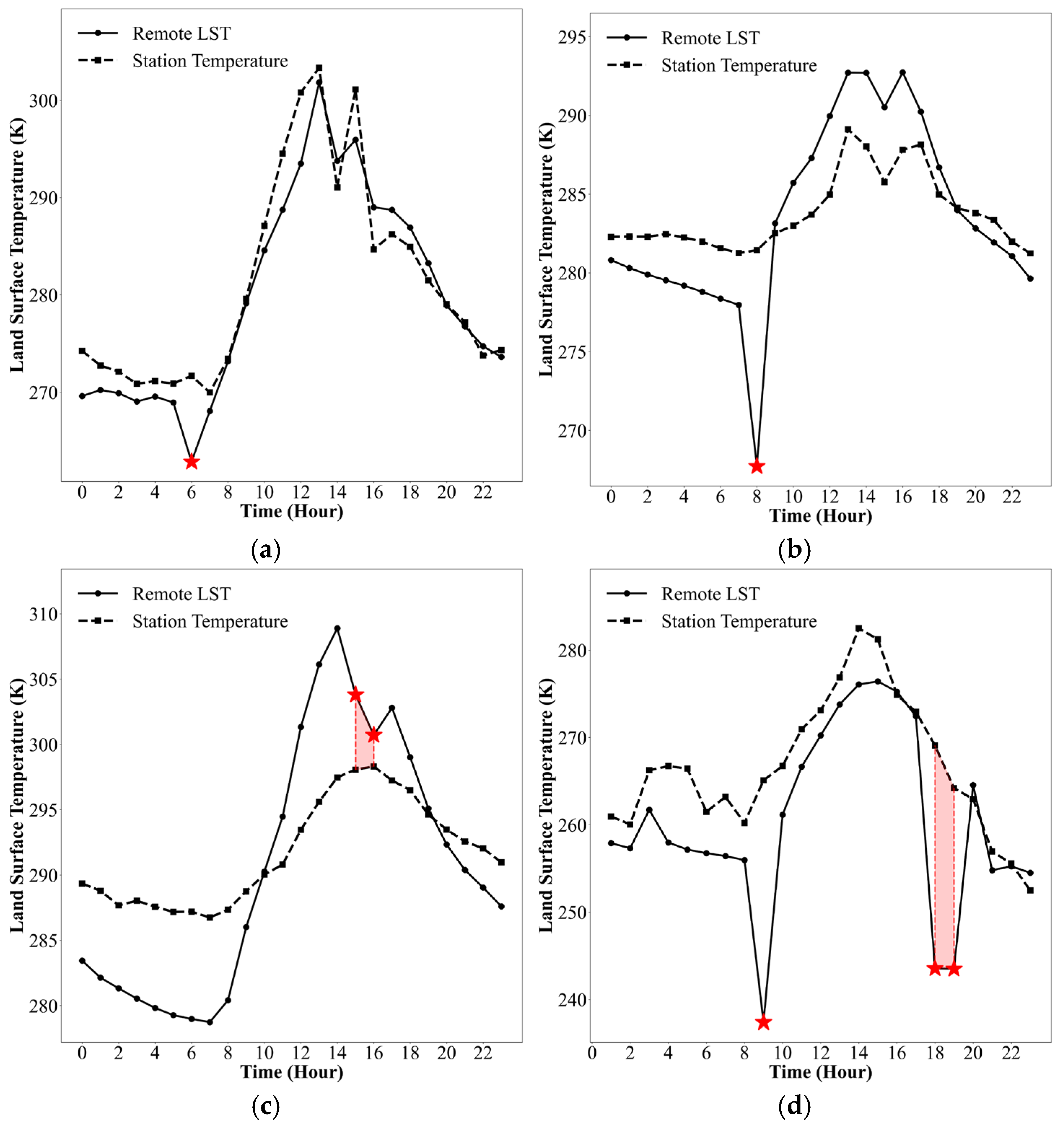
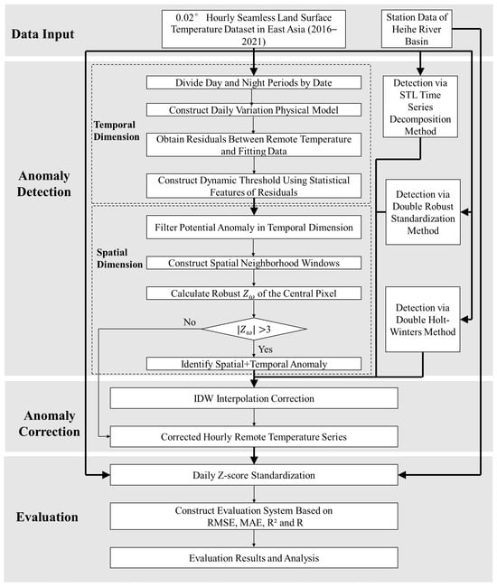
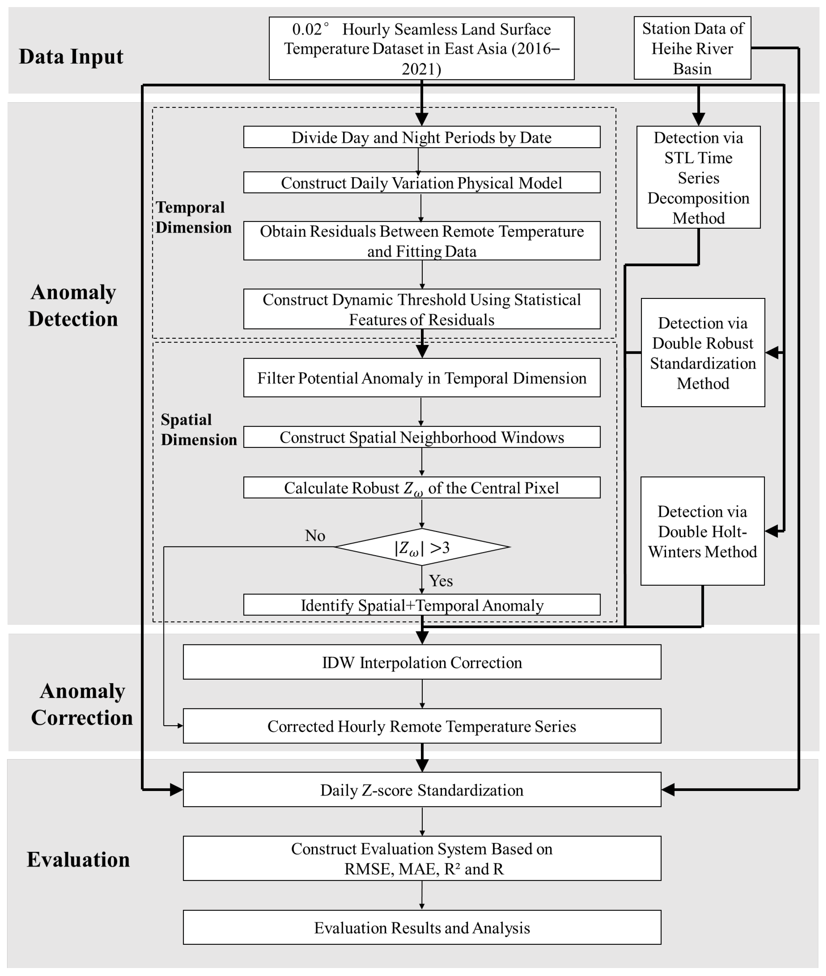
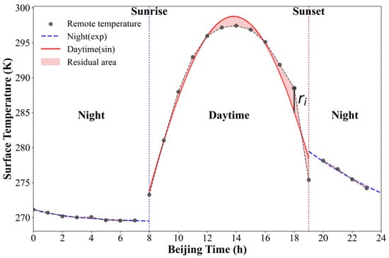
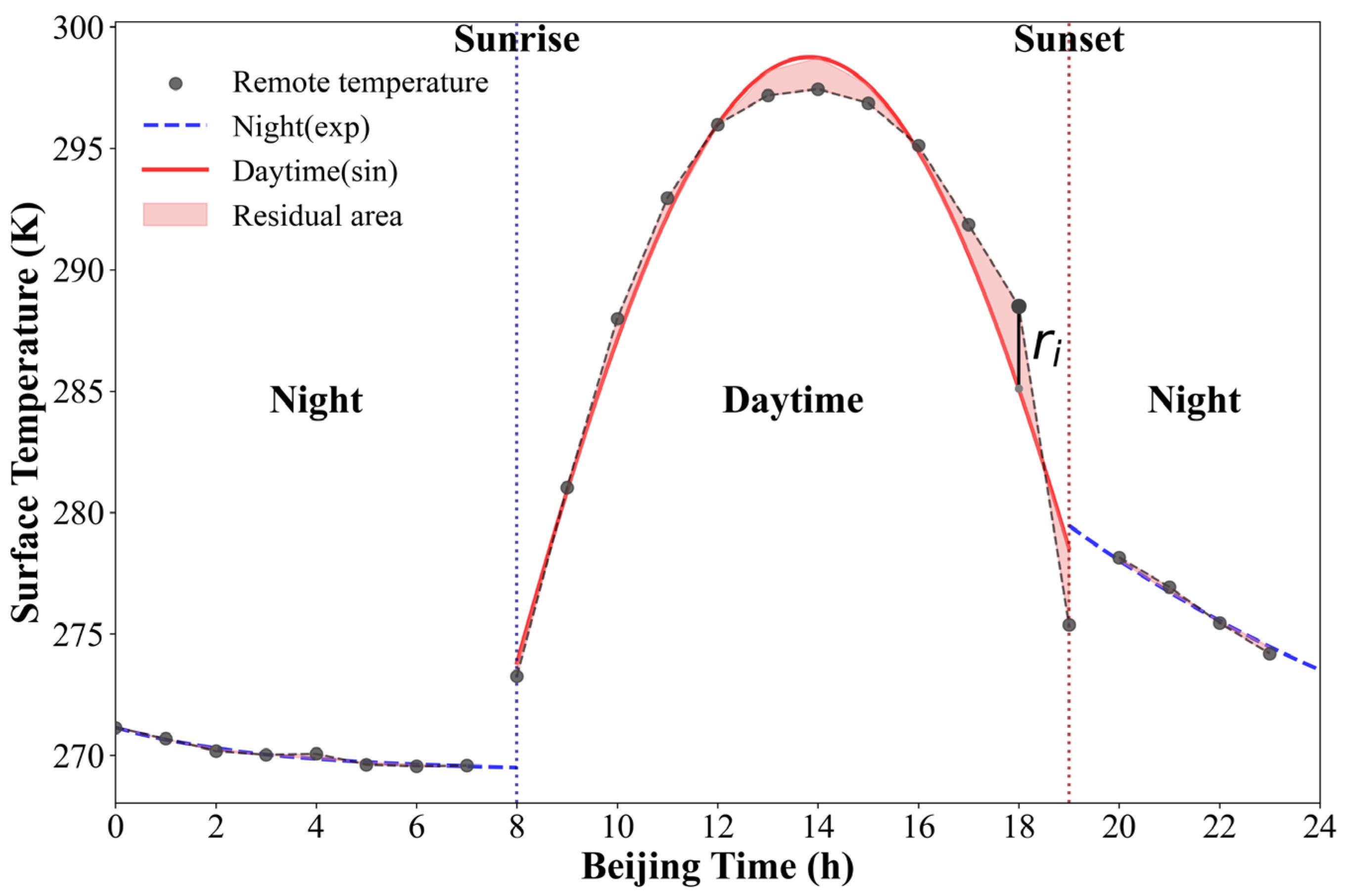
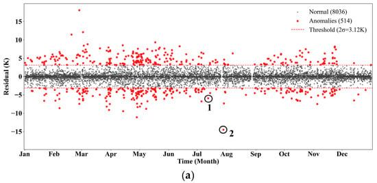
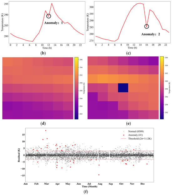
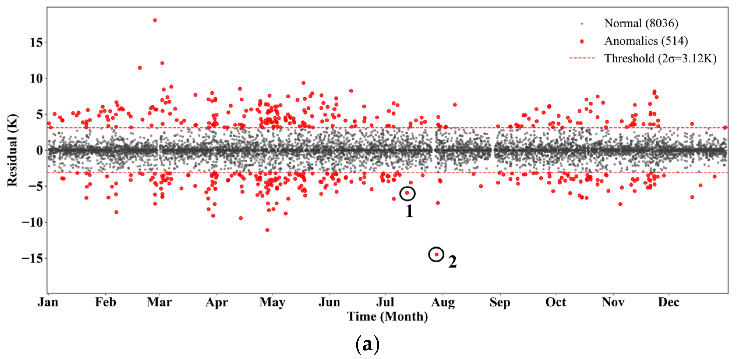
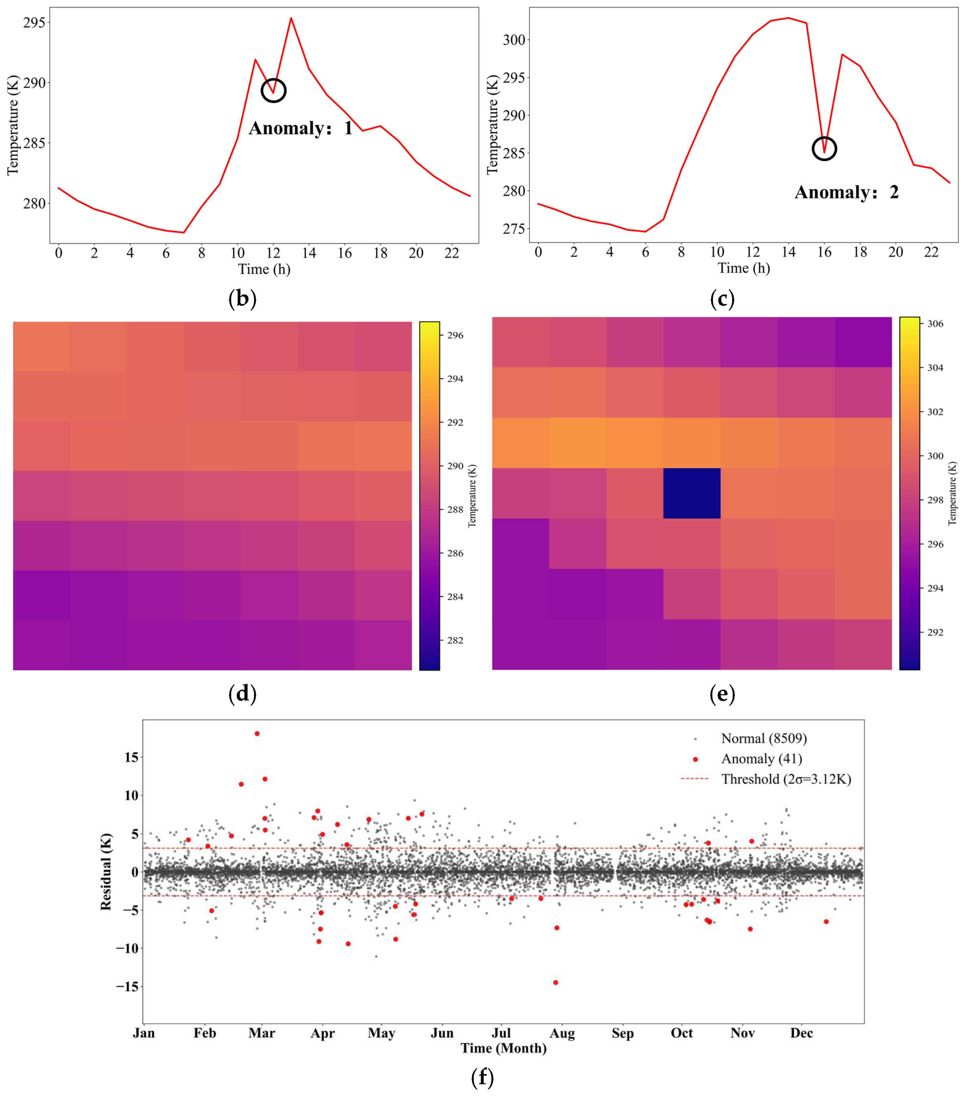
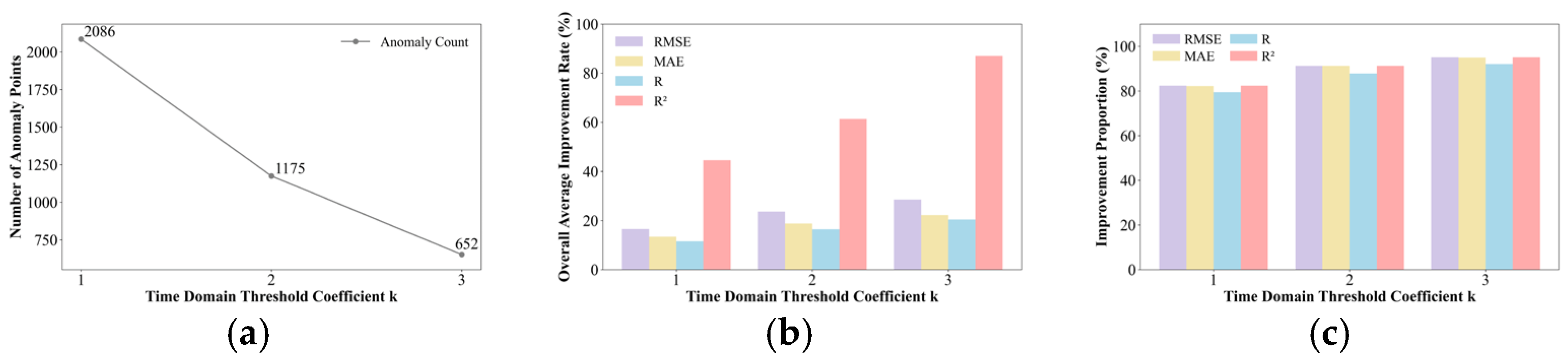
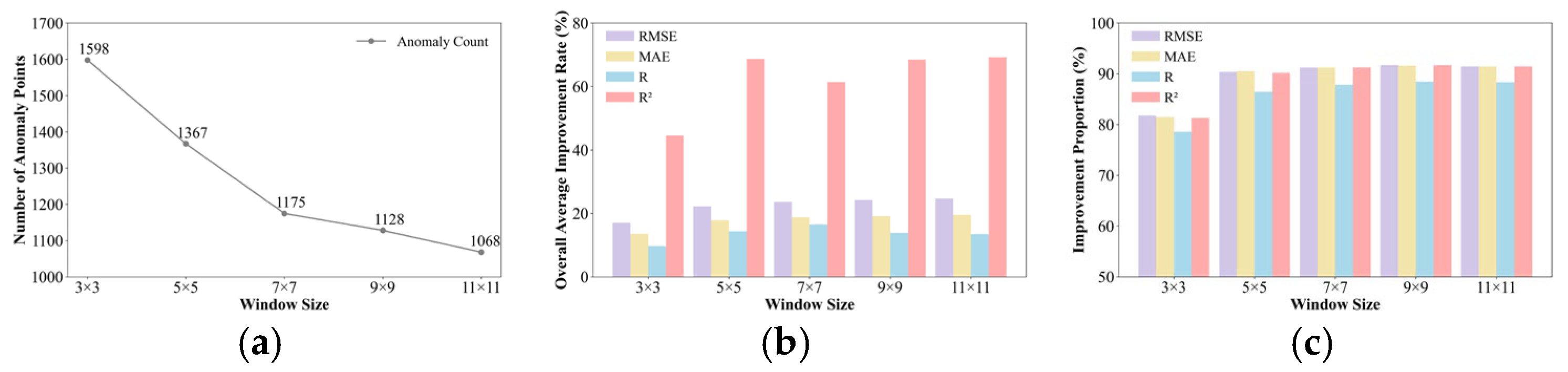
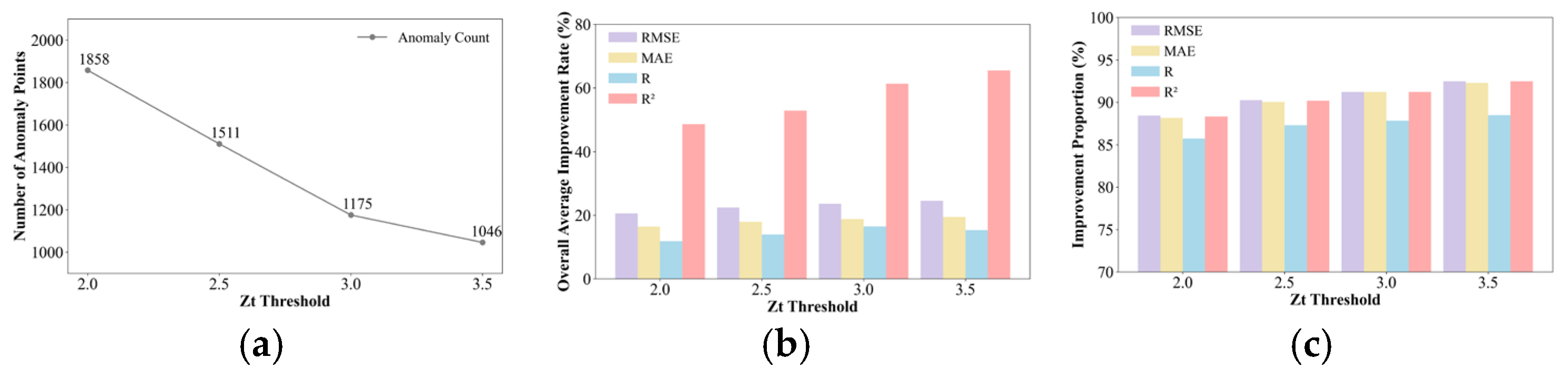
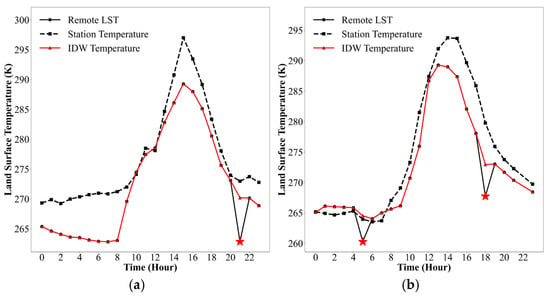
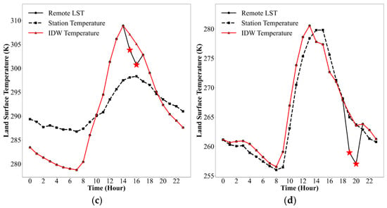
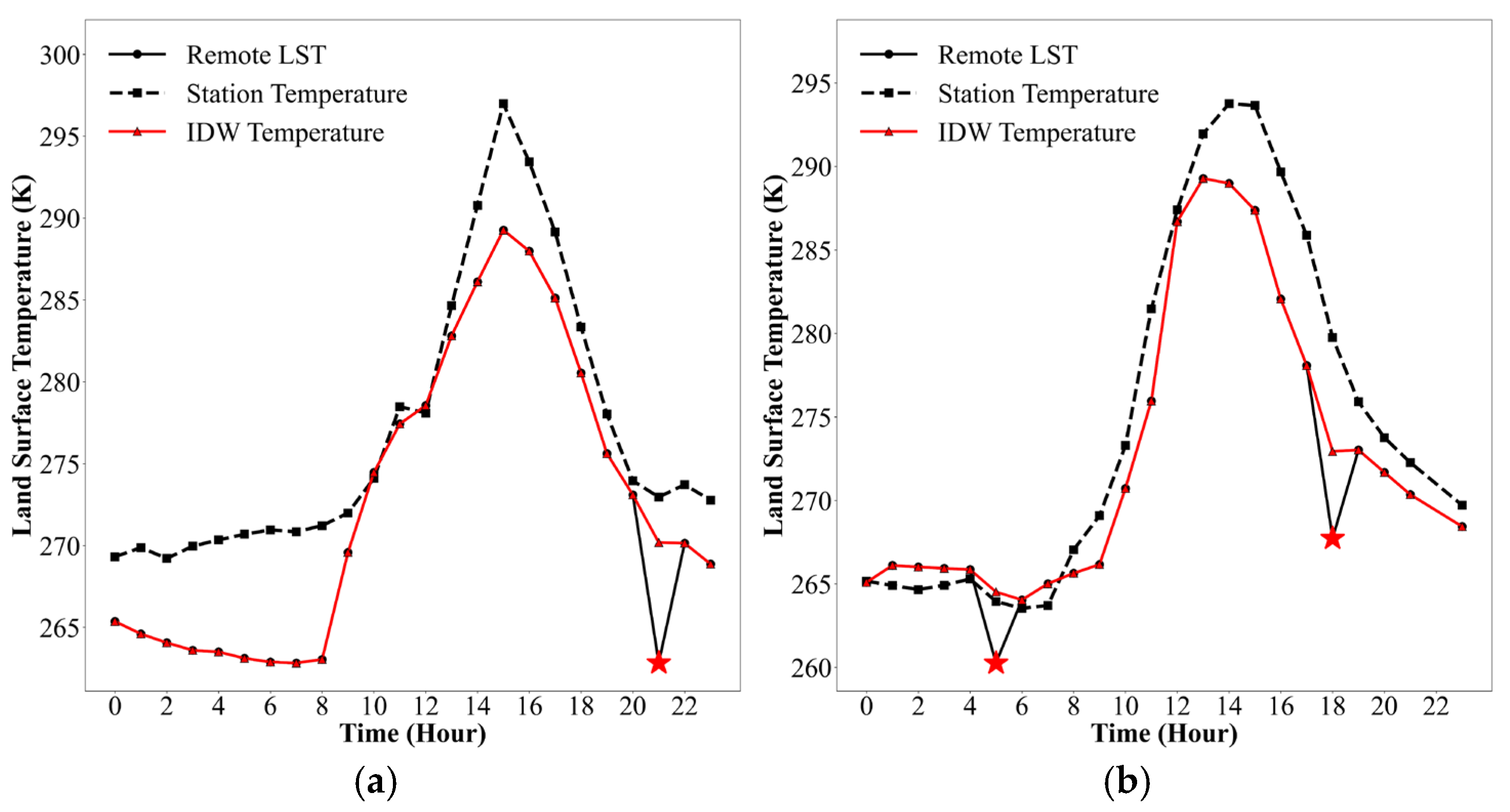
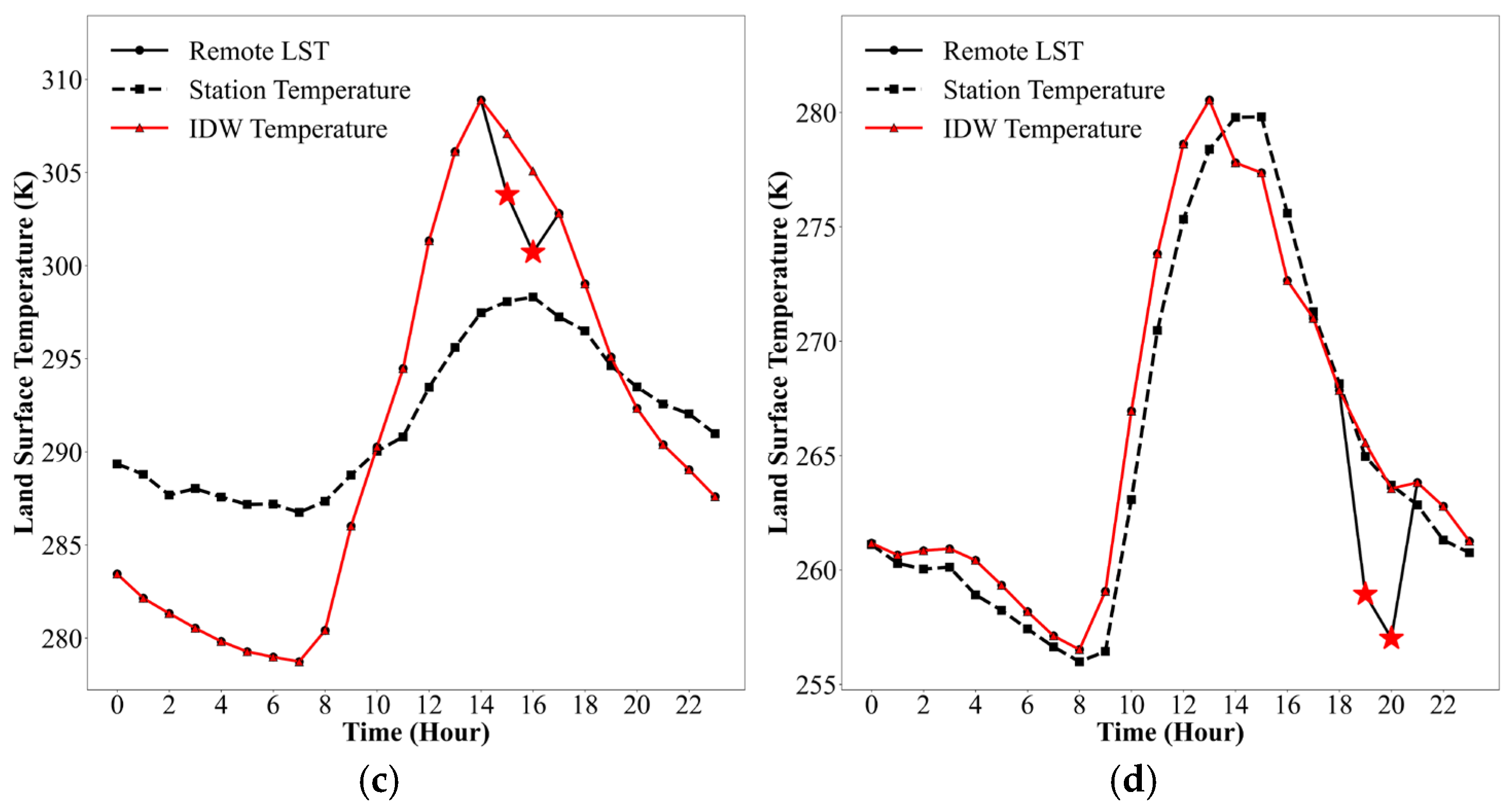
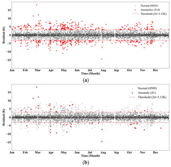
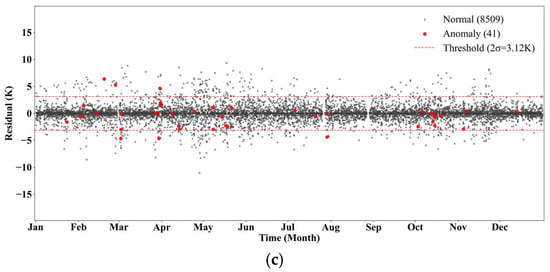
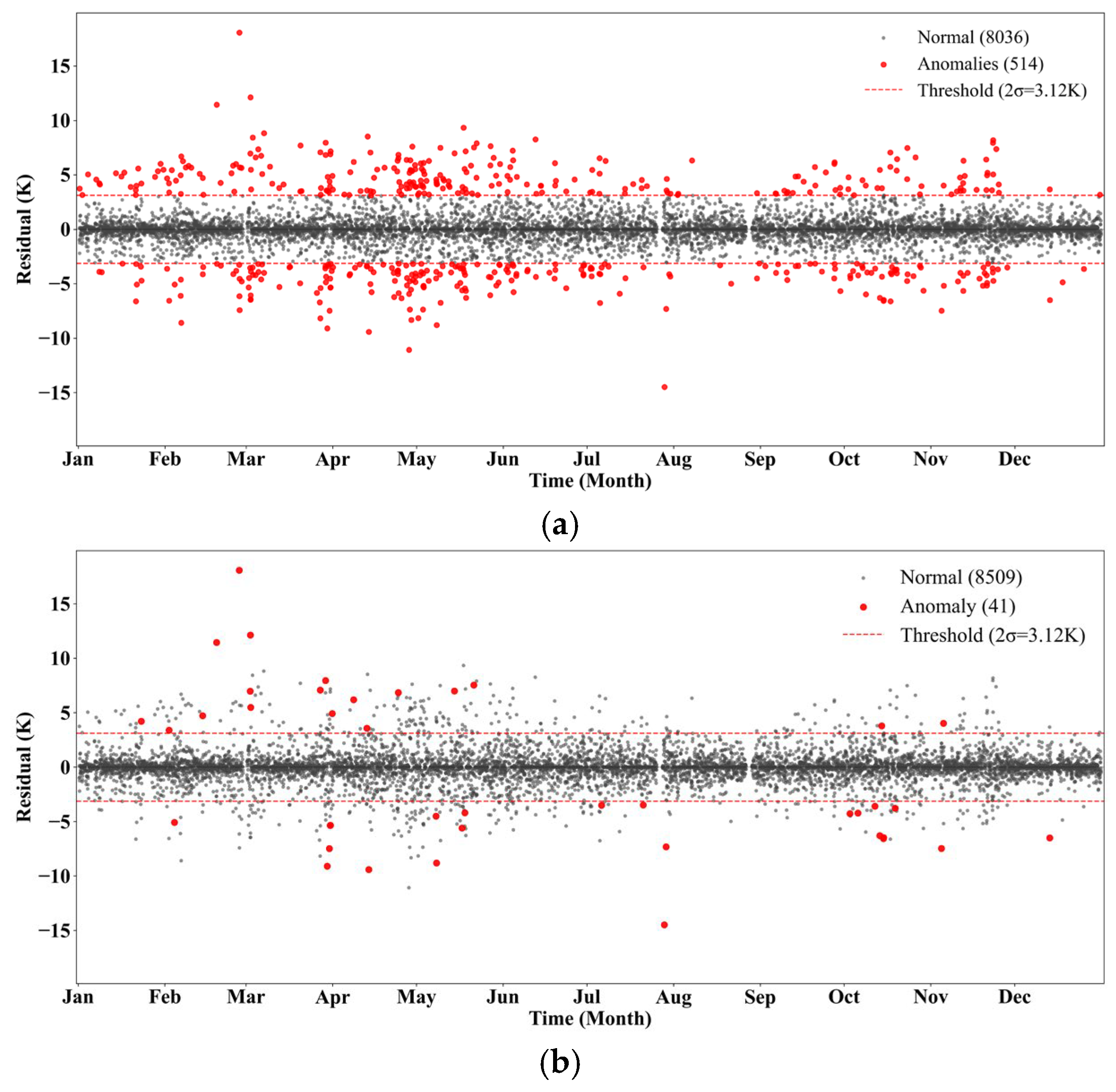
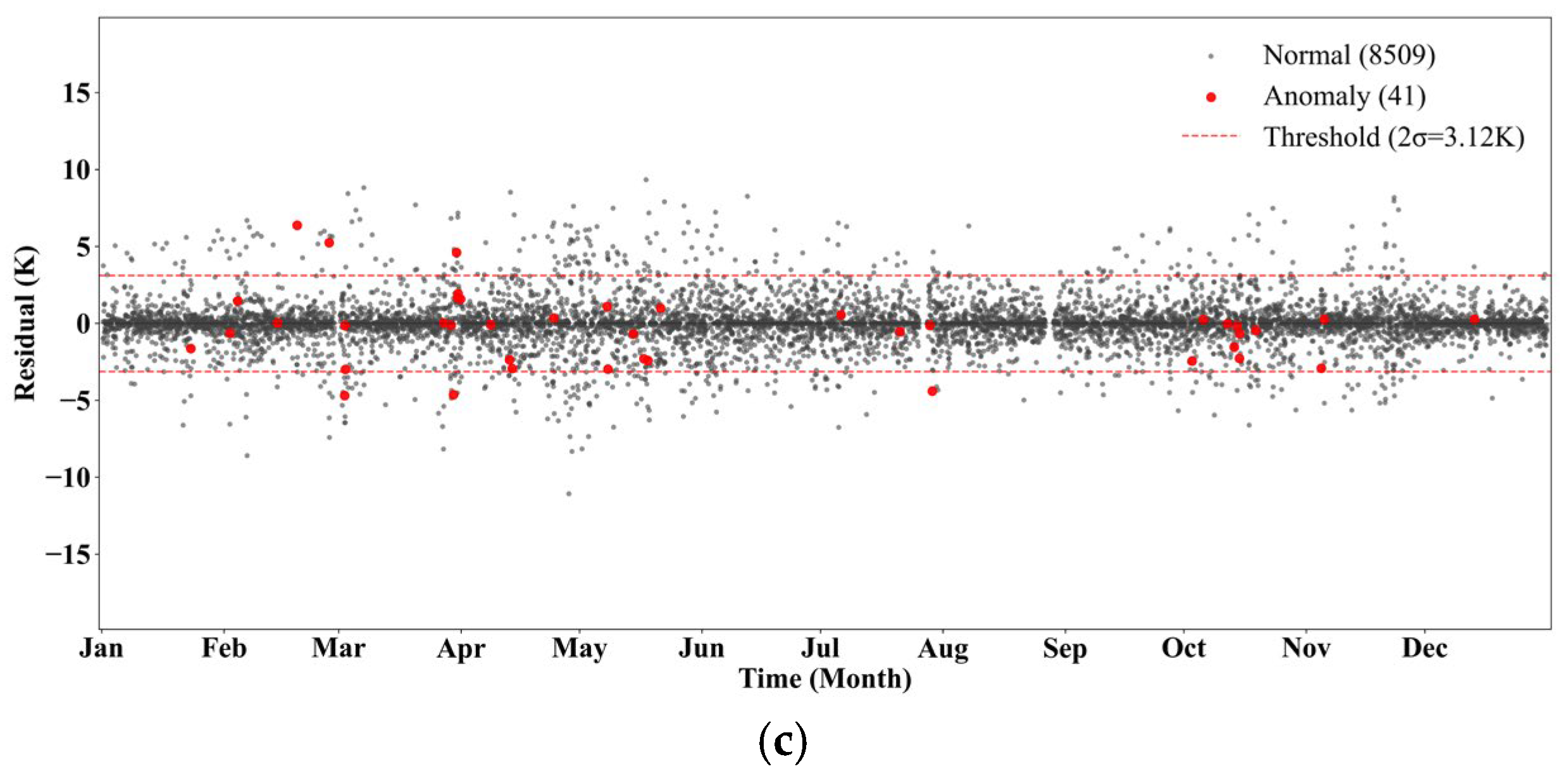
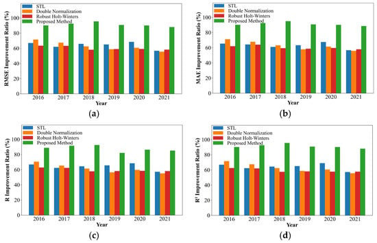
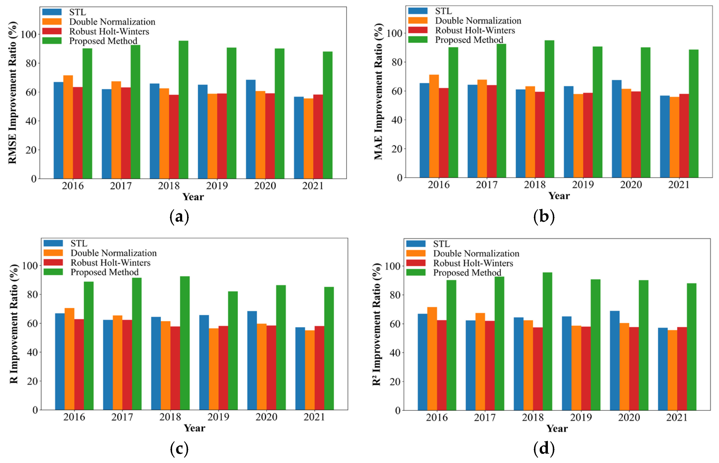
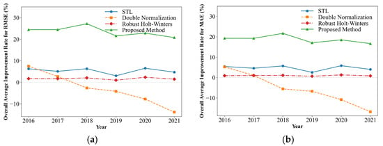
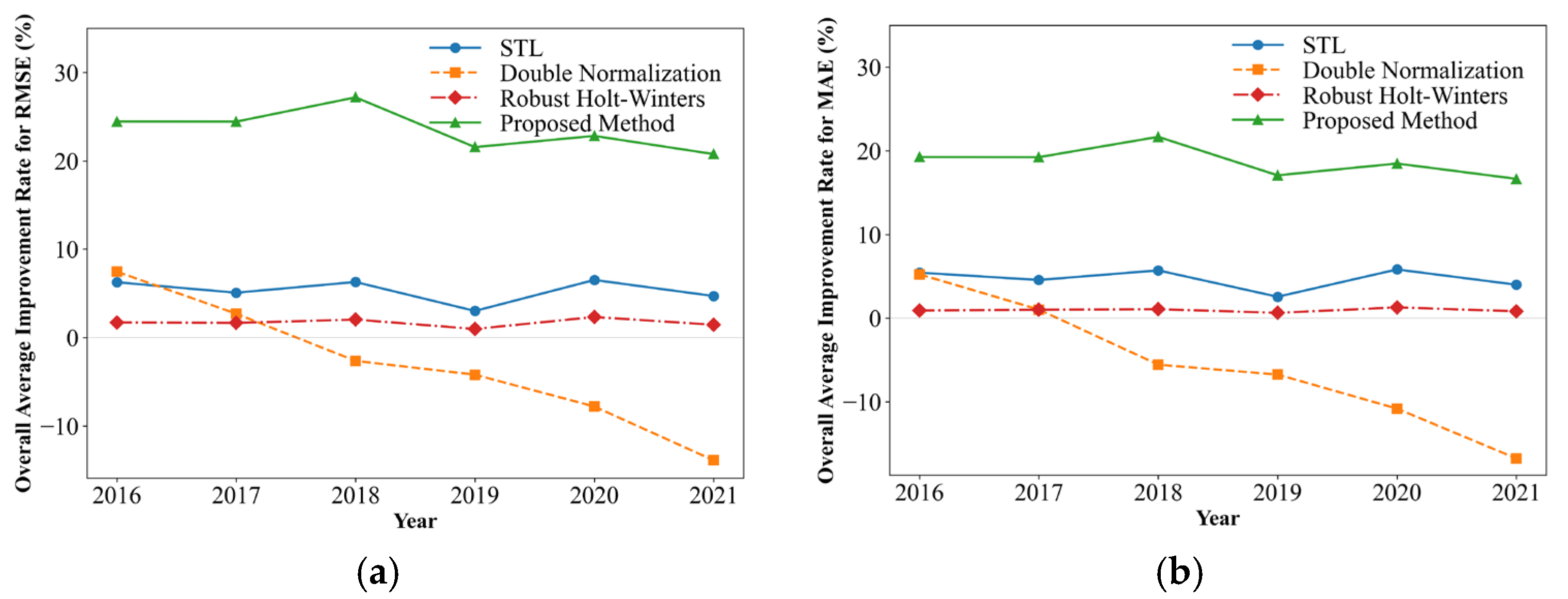
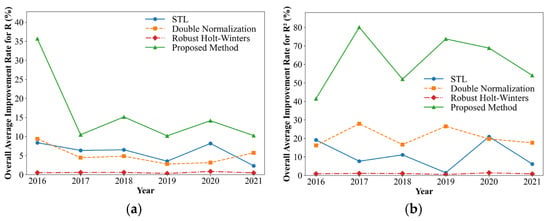
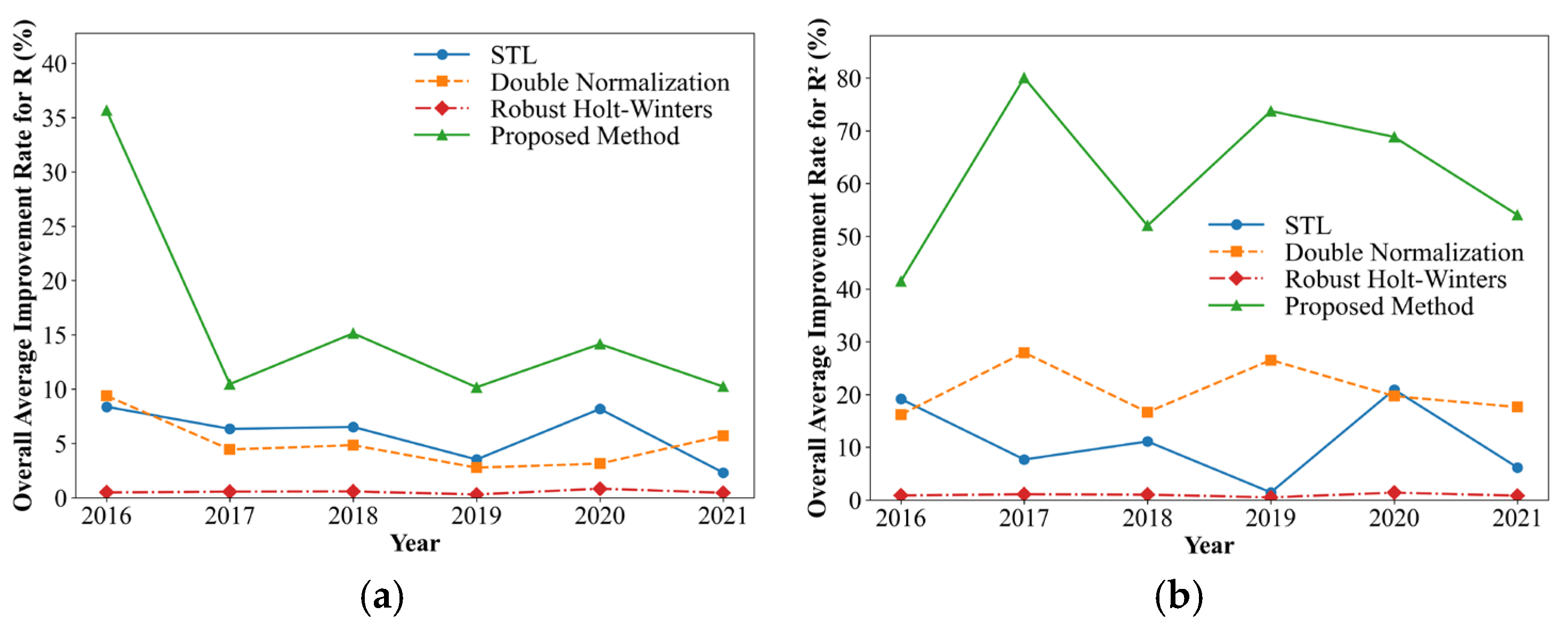

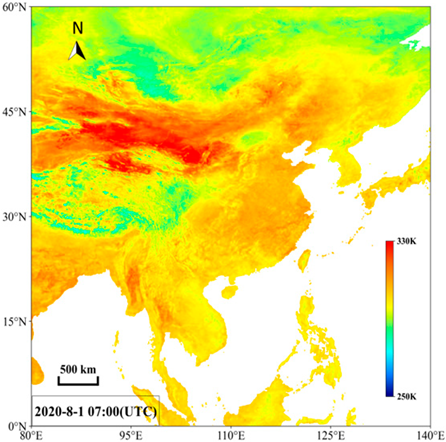
Disclaimer/Publisher’s Note: The statements, opinions and data contained in all publications are solely those of the individual author(s) and contributor(s) and not of MDPI and/or the editor(s). MDPI and/or the editor(s) disclaim responsibility for any injury to people or property resulting from any ideas, methods, instructions or products referred to in the content. |
© 2026 by the authors. Licensee MDPI, Basel, Switzerland. This article is an open access article distributed under the terms and conditions of the Creative Commons Attribution (CC BY) license.