Sea Surface Wind Speed Retrieval with a Dual-Branch Feature-Fusion Network Using GaoFen-3 Series SAR Data

Highlights

What are the main findings?

• The proposed attention-guided dual-branch feature-fusion network, which integrates spatial and nonlinear features from the GaoFen-3 (GF-3) series SAR satellite data, leads to an effective improvement in sea surface wind speed retrieval accuracy while maintaining the key spatial characteristics of the wind field.
• The refinement of radiometric calibration constants for specific GF-3B SAR satellite beam codes, achieved through a Geophysical Model Function (GMF)-based method, has successfully enhanced the accuracy of sea surface wind speed retrieval to meet international benchmarks.

What are the implications of the main findings?

• The development of an attention mechanism-guided, dual-branch feature-fusion model provides a new dimension for SAR wind speed retrieval by fusing nonlinear relationships and local spatial features through a parallel structure, capturing the inherent spatial characteristics of marine dynamics.
• A correction to the radiometric calibration constants for specific beam codes of the GF-3B SAR satellite was applied, using a GMF and scatterometer wind field data. This refinement addresses the insufficient radiometric accuracy that hindered sea surface wind speed retrieval.

Abstract

To address the suboptimal radiometric calibration accuracy observed in specific beam codes of the GaoFen-3 (GF-3) series satellite for sea surface wind speed (SSWS) retrieval, this study introduces a calibration constant correction method based on the geophysical model function (GMF). This approach enables high-precision SSWS retrieval from GF-3B data. Conventional SAR-based SSWS retrieval models typically rely on pointwise mapping relationships, which overlook the spatial characteristics inherent in dynamic sea surface wind fields. To overcome this limitation, this study proposes an attention-guided dual-branch feature-fusion network (ADBFF-NET). The first branch, implemented as a backpropagation neural network (BPNN), learns nonlinear mappings between the normalized radar cross-section (NRCS, σ⁰), incidence angle, azimuth look direction, and wind vectors (speed and direction). The second branch, designed as a residual convolutional neural network, extracts spatial features of wind fields. An attention mechanism fuses the outputs of both branches, thereby enhancing retrieval accuracy. Experiments conducted with GF-3 series satellite data were validated against the European Centre for Medium-Range Weather Forecasts (ECMWF) Reanalysis V5 (ERA5), Advanced Scatterometer (ASCAT) wind fields, and altimeter-derived wind speeds. The results indicate that the SSWS retrieved from GF-3B SAR data using the corrected calibration constants achieve a root mean square error (RMSE) of 1 m/s against ERA5 wind speeds, representing an approximately 40% reduction compared with the RMSE obtained using the original calibration constant. Furthermore, compared to ERA5 and ASCAT data, the RMSE of the wind speeds retrieved by the ADBFF-NET model reaches 1.17 m/s and 1.03 m/s, respectively.

1. Introduction

Synthetic Aperture Radar (SAR) satellites operate independently of atmospheric conditions such as clouds, rain, and fog, thereby enabling continuous, all-weather monitoring. This capability provides distinct advantages for retrieving marine dynamic parameters, including sea surface wind and wave fields. The C-SAR satellite constellation, with a spatial resolution of 1 m, consists of two satellites: C-SAR01 (GF-3B) and C-SAR02 (GF-3C), both sharing identical technical specifications. These satellites provide multipolarization, high-resolution, wide-swath quantitative remote sensing data for both land and ocean observations. With the operational deployment of this constellation, the GF-3 SAR satellite system now supports routine, high-resolution monitoring of sea surface wind fields over the South China Sea. Consequently, it enables timely and accurate acquisition of marine meteorological information, thereby enhancing maritime navigation safety and contributing to regional economic development.

Current approaches for retrieving SSWS from SAR data include empirical models, neural networks, theoretical models, and azimuth cutoff techniques. Among these, empirical models and neural networks are the most widely applied. Empirical models establish parameterized functional relationships between NRCS, SSWS, wind direction, radar incidence angle, and azimuth angle. In C-band SAR applications, GMFs, particularly the CMOD series, have been most extensively employed for SSWS retrieval. The European Space Agency (ESA) proposed CMOD4 in 1992 based on ERS-1 scatterometer analysis, establishing a mapping between NRCS and wind parameters. Validation studies confirmed its strong applicability to C-band SAR, with reliable performance at low wind speeds but systematic overestimation at medium-to-high wind speeds [1]. To address this limitation, CMOD5 was developed by optimizing CMOD4 using ERS-2 scatterometer data and first-guess winds from the ECMWF, significantly improving retrieval accuracy for wind speeds above 10 m/s [2]. Further refinement produced CMOD5.N, which optimized 28 parameters in CMOD5 through joint analysis of ERS-2 scatterometer and ASCAT wind field data, improving wind speed retrieval accuracy by approximately 0.7 m/s [3]. For GF-3 SAR data, CMOD5.N similarly demonstrates enhanced performance [4]. By minimizing the cost function between NRCS and ECMWF model wind fields, wind vectors were retrieved, yielding an RMSE of 2.34 m/s for VV-polarization wind speed retrievals [5]. To mitigate the influence of varying atmospheric density on wind field retrieval, CMOD6 and CMOD7 were subsequently developed based on cross-calibrated ESCAT and ASCAT data and 10 m equivalent neutral winds, comprehensively improving key wind field quality metrics compared with CMOD5.N [6,7]. For C-band horizontal-horizontal (HH) polarization SAR data, wind speed retrieval typically involves converting HH-polarized NRCS to VV-polarized NRCS equivalents using a polarization ratio (PR) model, followed by application of GMF. Alternatively, the CMODH directly supports wind retrieval from HH-polarized SAR data [8]. Empirical studies further confirm that at wind speeds above 20 m/s, cross-polarized (HV/VH) SAR NRCS exhibits a predominantly linear dependence on wind speed with minimal sensitivity to wind direction [9]. Consequently, cross-polarization SAR retrievals achieve higher accuracy than co-polarized data, providing a critical supplement for high-wind-speed inversion [10].

Neural networks leverage powerful nonlinear mapping capabilities to establish input-output relationships through iterative processes, proving effective for SSWS and wave parameter retrieval [11]. Based on ERS-1 scatterometer data, a feedforward neural network known as Quasi-linear Multi-layered Network (QMN) was proposed. It employs a cascaded module design to perform wind speed retrieval, wind direction classification, and ambiguity removal, representing the first neural-network-based implementation of the complete scatterometer wind field retrieval workflow. This approach demonstrated significant advantages over traditional methods in terms of accuracy, robustness, and efficiency [12]. Subsequent studies further validated that end-to-end learning of the inverse mapping relationship within CMOD4 using neural networks effectively resolves issues of solution multiplicity and noise sensitivity in scatterometer wind field retrieval. Its accuracy and scalability provide a solid foundation for operational applications [13,14]. For SSWS retrieval from SAR data, Horstmann et al. developed a three-layer feedforward neural network by fusing ERS-1/2 and ENVISAT SAR wave mode data with scatterometer and meteorological model wind fields. The retrieved wind speeds achieved an RMSE of 0.93 m/s compared with scatterometer measurements, significantly outperforming CMOD4 [15]. Meanwhile, BPNNs strengthen nonlinear modeling through gradient-based optimization. BPNN-based studies have extensively explored SAR wind retrieval, including a GMF-guided model for Sentinel-1 HH-polarized data in Arctic waters [16], and a BP model that corrected biases in Sentinel-1 wind speed retrievals using NDBC buoy data [17], both demonstrating superior performance at medium-to-high wind speeds. Unlike the pointwise mapping of BPNNs, convolutional neural networks (CNNs) exploit spatial features through local connectivity and weight sharing. A deep residual CNN model showed promising results in retrieving SSWS and significant wave heights from Sentinel-1 dual-polarized SAR data, achieving a wind speed RMSE of 1.9 m/s [18]. This validates the feasibility of residual networks for retrieving marine dynamic parameters from SAR data. Even under typhoon conditions, a DenseNet model trained on Sentinel-1 dual-polarized SAR data achieved an RMSE of 1.74 m/s for wind speed retrieval without requiring external wind field inputs [19]. Furthermore, the spatial feature extraction capability of CNNs enables effective identification of rainfall intensity from SAR data and subsequent correction of rain-contaminated wind retrievals, reducing the RMSE to 1.76 m/s after correction [20]. Utilizing GF-3 quad-polarized data, Shao et al. developed a wind direction retrieval model that operates independently of external information, achieving an RMSE of 17.7°. This provides a novel solution for retrieving sea surface wind fields relying solely on SAR data [21].

Neural network models currently employed for SAR-derived SSWS retrieval primarily rely on BPNNs and CNNs. However, BPNNs are inherently restricted to point-to-point nonlinear mappings and thus struggle to capture the spatial distribution characteristics of sea surface wind fields. Although CNNs can extract spatial information, their conventional fixed-window processing often smooths fine-grained details within the wind speed field, ultimately limiting retrieval accuracy. To address these limitations, this study proposes an attention-guided dual-branch feature-fusion neural network. The model is designed to synergistically exploit nonlinear features and local spatial contextual information from SAR data, thereby enabling high-precision inversion of SSWS from C-band SAR imagery.

2. Data and Preprocessing

2.1. SAR Data

The GF-3 series SAR satellite provides twelve imaging modes, classified into five operational categories: Spotlight, Stripmap, Ultra-Fine Stripmap, ScanSAR, and Wave Mode. The Stripmap category comprises five sub-modes: Fine Stripmap 1 (FSI), Fine Stripmap 2 (FSII), Standard Stripmap (SS), Quad-Polarization Stripmap 1 (QPSI), and Quad-Polarization Stripmap 2 (QPSII) [22]. For SSWS retrieval from GF-3B data, this study employed 490 images in QPSI and QPSII modes, acquired between April 2023 and September 2025, with most covering the South China Sea and adjacent waters. To meet the requirements of neural network training and reduce the risk of overfitting, an additional 2117 images from the GF-3 series, collected between May 2017 and October 2024, were incorporated. In total, the dataset consists of 2607 images. The spatial distribution of these data is presented in Figure 1.

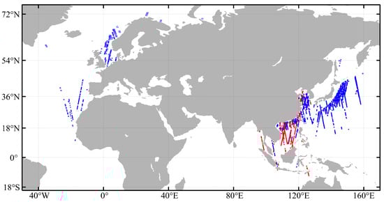
Figure 1. Spatial Distribution of GF-3 series SAR Data Used in This Study. The red box denotes GF-3B satellite data, and the blue box denotes GF-3 satellite data.

The image-related parameters of the four imaging modes used in this paper are shown in Table 1.

Table 1. Technical Parameters of GF-3 Satellite Imaging Modes.

No.	Imaging Mode	Resolution (m)		Swath Width (km)	Polarization
		Azimuth	Range
1	QPSI	8	6~9	30	Quad-Polarization
2	QPSII	25	15~30	40	Quad-Polarization
3	FSI	5	4~6	50	Dual-polarization
4	FSII	10	8~12	100	Dual-polarization

2.2. ERA5 Reanalysis Wind Field Data

The ERA5 dataset, developed by the ECMWF, represents the latest fifth-generation global atmospheric reanalysis product. It provides a wide range of surface and atmospheric parameters, including equivalent neutral wind field components at 10 m above sea level, stored as the u- and v-components of wind. The dataset features a spatial resolution of 0.25° and a temporal resolution of 1 h. ERA5 reanalysis wind fields have been extensively applied in SSWS retrieval and validation studies.

2.3. ASCAT Wind Field Data

The ASCAT is an instrument designed for ocean surface wind retrieval. It employs three vertically polarized antennas operating at 5.255 GHz, configured at 45°, 90°, and 135° relative to the satellite track. ASCAT instruments are carried on three satellites: MetOp-A (launched in 2006, designated ASCAT-A), MetOp-B (2012, ASCAT-B), and MetOp-C (2018, ASCAT-C) [23].

Research indicates that ASCAT wind data exhibit high accuracy and stability, which have been validated through multiple approaches such as ship-based lidar, offshore platform observations, and reanalysis data, demonstrating high reliability in offshore regions [24]. These data can effectively improve the accuracy of wind fields in mesoscale numerical simulations through assimilation methods and serve as a reliable input source [25,26]. Furthermore, the three ASCATs onboard the MetOp-A/B/C satellites have undergone rigorous cross-calibration, ensuring the consistency and stability of the wind products over long-term time series, thereby providing dependable support for SSWS retrieval research and validation using SAR data [27,28]. This study uses daily gridded wind products (0.25° resolution) from all three ASCAT sensors, obtained from Remote Sensing Systems. The dataset includes: UTC time, ocean surface wind speed/direction, rain flag, and sum-of-squares parameters.

2.4. Altimeter Wind Speed Data

The ERA5 wind field data and ASCAT wind field data used in this study both feature a spatial resolution of 0.25°. To validate the accuracy of the proposed wind speed retrieval model at higher spatial resolutions, wind speed measurements from six satellite altimeters were utilized. These altimeters include Jason-3, CryoSat-2, SARAL/AltiKa, CFOSAT, HY-2B, and Sentinel-6A. The altimeter data are sourced from the Wave Thematic Assembly Center (WAVE-TAC) multi-mission processing system, which provides homogenized near-real-time along-track significant wave height (SWH) products. An important characteristic of this product is its built-in consistency. Data from all missions are calibrated against a common reference mission, subjected to uniform quality control procedures such as surface/ice flagging and parameter threshold checks, and filtered along-track. For the purposes of this study, the associated altimeter wind speeds, derived from the respective Level-2 algorithms, are integrated into these processed files. The final product for each mission is generated using identical 3 h temporal windows and file formats. As a result, the wind speed data obtained from the different altimeters are intrinsically consistent in terms of spatiotemporal reference and quality, and they provide gridded data with an effective spatial resolution of approximately 7 km. Previous studies have confirmed the reliability of such altimeter-based wind speed products, reporting RMSE values typically below 1.5 m/s when compared with buoy measurements [29,30].

2.5. Data Preprocessing

This study employs Level-1A Single Look Complex (SLC) products from the GF-3 series satellite. Prior to SSWS retrieval, data preprocessing and spatiotemporal matching with external wind field datasets are required. The preprocessing workflow includes:

2.5.1. Radiometric Calibration

The acquisition of scattering information from ground targets is a prerequisite for the quantitative inversion of SAR data. A critical step in this process is radiometric calibration. Absolute radiometric calibration establishes a quantitative relationship between the digital signals measured by the remote sensing detector and the corresponding actual radiant energy, thereby converting the digital number (DN) values in SAR images into the physical scattering properties of surface targets. The radiometric calibration formula implemented for the GF-3 series satellite is presented in Equation (1).

$${\mathsf{\sigma }}_{\mathrm{d}\mathrm{B}}^0=10\log \left({\mathrm{P}}^{\mathrm{I}}\times {\left(\mathrm{Q}\mathrm{u}\mathrm{a}\mathrm{l}\mathrm{i}\mathrm{f}\mathrm{y}\mathrm{V}\mathrm{a}\mathrm{l}\mathrm{u}\mathrm{e}/\mathrm{32,767}\right)}^2\right)-{\mathrm{K}}_{\mathrm{d}\mathrm{B}}$$

(1)

where ${\mathsf{\sigma }}_{\mathrm{d}\mathrm{B}}^0$ is the NRCS, ${\mathrm{P}}^{\mathrm{I}}$ is the squared magnitude of the complex data, $\mathrm{Q}\mathrm{u}\mathrm{a}\mathrm{l}\mathrm{i}\mathrm{f}\mathrm{y}\mathrm{V}\mathrm{a}\mathrm{l}\mathrm{u}\mathrm{e}$ denotes the maximum value prior to quantization for the current image, corresponding to the value of the metadata field ‘QualifyValue’, ${\mathrm{K}}_{\mathrm{d}\mathrm{B}}$ is the radiometric calibration constant, corresponding to the value of the metadata field ‘CalibrationConst’.

2.5.2. Image Homogeneity Test

During SSWS retrieval from SAR data, phenomena such as oil slicks and sea ice modify the radar scattering characteristics of the ocean surface, thereby degrading wind speed inversion accuracy. To mitigate this effect, a homogeneity test is typically applied to exclude anomalous regions. This study adopts the coefficient of variation, computed as the ratio of the local standard deviation to the image mean, as the homogeneity index, given in Equation (2).

$$\left\{{\displaystyle \begin{array}{c}{\mathsf{\xi }}_{\mathrm{H}}={\left({\displaystyle \sum _{\mathrm{k}}}\stackrel{-}{\mathrm{mean}}({\widehat{\mathsf{\Phi }}}_{\mathrm{k}})\right)}^{-1}{\displaystyle \sum _{\mathrm{k}}}{\displaystyle \frac{\stackrel{-}{\mathrm{var}}({\widehat{\mathsf{\Phi }}}_{\mathrm{k}})}{\stackrel{-}{\mathrm{mean}}({\widehat{\mathsf{\Phi }}}_{\mathrm{k}})}}\\ \stackrel{-}{\mathrm{var}}({\widehat{\mathsf{\Phi }}}_{\mathrm{k}})={\displaystyle \frac{1}{\mathrm{N}}}{\displaystyle \sum _{\mathrm{j}=1}^{\mathrm{N}}}{({\widehat{\mathsf{\Phi }}}_{\mathrm{k}}^{\mathrm{j}})}^2- \mathrm{m}\mathrm{e}\mathrm{a}\mathrm{n}{({\widehat{\mathsf{\Phi }}}_{\mathrm{k}})}^2\end{array}}\right.$$

(2)

where ${\widehat{\mathsf{\Phi }}}_{\mathrm{k}}$ denotes the power spectral value for each sub-image, and ${\mathsf{\xi }}_{\mathrm{H}}$ represents the homogeneity index. Images with ${\mathsf{\xi }}_{\mathrm{H} }$ ≤ 1.05 are classified as homogeneous sea surfaces and prepared for subsequent space-time matching with sea surface wind field data.

2.5.3. Space-Time Matching

Given the substantial disparity in spatial resolution between GF-3 image and external wind field datasets, the SAR data were downsampled to a spatial resolution of 2 km, producing sub-images with a tile size of 2 km × 2 km. These sub-images were subsequently subjected to spatiotemporal matching with the wind field data. The detailed workflow of this matching process is illustrated in Figure 2.

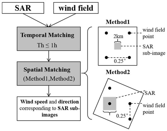
Figure 2. Workflow of Space-Time Matching Between SAR and Wind Field Data.

• Temporal Matching

SAR data were temporally matched with ERA5 and ASCAT wind field products using a threshold (Th) of 1 h as the maximum allowable temporal difference. In addition, altimeter-derived wind speed products with a temporal resolution of 3 h were incorporated into this study. For these altimeter datasets, temporal matching was performed by selecting records corresponding to the SAR observation time window.

2.

Spatial Matching

Spatial matching assigns corresponding wind speed and direction information to SAR sub-images. Two approaches were employed:

Method 1: The wind direction and speed at the location corresponding to the SAR sub-image are obtained by interpolating the four nearest wind field grid points surrounding the sub-image. During wind speed interpolation, the u- and v-components were separately interpolated to ensure accuracy.

Method 2: The SAR NRCS corresponding to a wind field point is obtained by calculating the mean value of the SAR sub-image within a defined range surrounding that point, thereby establishing the correspondence between SAR parameters and wind field parameters.

Method 1 yields a large number of SAR-wind field matched pairs suitable for network training. However, Method 2 provides higher accuracy when substantial resolution disparities exist between SAR and wind field data. Accordingly, Method 2 was adopted in Section 3.2 and Section 4.3.2 for comparative experiments with ASCAT and altimeter-derived wind products.

3. Radiometric Calibration Constants Correction for GF-3B Data Based on GMF

The accuracy of SAR radiometric calibration directly affects the precision of quantitative retrieval results. Therefore, prior to SSWS retrieval, we validated the radiometric calibration accuracy of the collected GF-3B data using the CMOD5.N model.

3.1. Radiometric Calibration Accuracy Verification for GF-3B Data

CMOD5.N establishes an empirical GMF relating C-band NRCS to incidence angle, radar look direction, and the 10 m wind vector, as formulated in Equation (3). Given wind speed and direction at 10 m, together with the radar incidence angle and look direction, the corresponding C-band NRCS can be computed.

$${\mathsf{\sigma }}_{\mathrm{v}\mathrm{v}}^0\left(\mathsf{\theta },\mathrm{\varnothing },{\mathrm{u}}_{10}\right)={\mathrm{a}}_{\mathrm{v}\mathrm{v}}^0\left(\mathsf{\theta },{\mathrm{u}}_{10}\right)\left[1+{\mathrm{a}}_{\mathrm{v}\mathrm{v}}^1\left(\mathsf{\theta },{\mathrm{u}}_{10}\right)\cos \mathrm{\varnothing }+{\mathrm{a}}_{\mathrm{v}\mathrm{v}}^2\left(\mathsf{\theta },{\mathrm{u}}_{10}\right)\cos 2\mathrm{\varnothing }\right]$$

(3)

where ${\mathsf{\sigma }}_{\mathrm{v}\mathrm{v}}^0$ denotes the VV-polarized NRCS; coefficient ${\mathrm{a}}_{\mathrm{v}\mathrm{v}}^{\mathrm{i}}$ is a function of both the wind speed at 10 m above the sea surface ${\mathrm{u}}_{10}$ and the radar incidence angle $\mathsf{\theta }$; $\mathrm{\varnothing }$ represents the angle between the wind direction and the radar look direction.

According to current international standards, SAR-retrieved SSWS must exhibit a bias of less than 0.5 m/s. Under this requirement, Zhang et al. [31] employed the CMOD5.N model to analyze the variation trends of VV-polarized NRCS bias (i.e., radiometric calibration accuracy range) under upwind (azimuth angle 0°) and crosswind (azimuth angles 90° and 270°) conditions, within incidence angles of 20–50° and wind speeds of 2–20 m/s. Their results indicate that a minimum radiometric calibration accuracy of 1.31 dB is necessary for C-band SAR systems to achieve wind speed retrievals with a bias below 0.5 m/s.

Based on the CMOD5.N model, this study validated the radiometric calibration accuracy using 490 GF-3B satellite QPSI/QPSII mode VV-polarized images. ERA5 wind speed and direction were utilized as simulated true values. Combining known radar incidence angles and radar look direction, the normalized radar NRCS (${\mathsf{\sigma }}_{\mathrm{v}\mathrm{v}}^{0\mathrm{\prime }}$) was calculated for each image via the CMOD5.N model. The NRCS (${\mathsf{\sigma }}_{\mathrm{v}\mathrm{v}}^0$) was derived by applying the officially released radiometric calibration constants of the GF-3B satellite to the corresponding images. The NRCS variation ${∆\mathsf{\sigma }}_{\mathrm{v}\mathrm{v}}^0$ (defined as ${∆\mathsf{\sigma }}_{\mathrm{v}\mathrm{v}}^0={\mathsf{\sigma }}_{\mathrm{v}\mathrm{v}}^{0\mathrm{\prime }}$ −${\mathsf{\sigma }}_{\mathrm{v}\mathrm{v}}^0$) was then computed, with results illustrated in Figure 3.

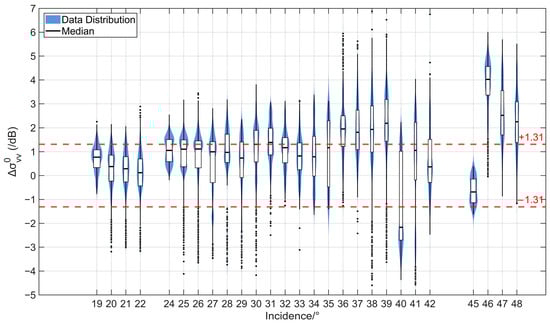
Figure 3. Variation of ${∆\mathsf{\sigma }}_{\mathrm{v}\mathrm{v}}^0$ with Incidence. The blue portions represent the kernel density estimation (KDE) curves of ${∆\mathsf{\sigma }}_{\mathrm{v}\mathrm{v}}^0$ for each incidence angle range (which are symmetric about the center); the white boxes represent the interquartile range (IQR) of the data, and the thick black line inside each box indicates the median of the data.

In Figure 3, the data distribution of ${∆\mathsf{\sigma }}_{\mathrm{v}\mathrm{v}}^0$ is represented by the blue shaded areas, with the median values indicated by the bold black central lines. The standard thresholds for radiometric calibration accuracy are marked by the horizontal red dashed lines at ±1.31 dB. Based on the analysis of the GF-3B QPSI/QPSII mode data processed with the CMOD5.N model, for incidence angles below approximately 35°, the high-density core of the ${∆\mathsf{\sigma }}_{\mathrm{v}\mathrm{v}}^0$ variation distribution lies predominantly within the acceptable range bounded by the ±1.31 dB thresholds, despite the presence of statistical outliers. Notably, as the incidence angle increases, a clear deviation emerges. Specifically, within the incidence angle ranges of 36–39° and 46–48°, the entire high-density core, along with the median value, shifts significantly above the +1.31 dB threshold. This deviation demonstrates that the inherent radiometric calibration accuracy of the dataset is insufficient to meet the requirement for SSWS retrievals with a bias target of less than 0.5 m/s. Consequently, correcting the radiometric calibration constants is a necessary preprocessing step before performing wind speed retrieval.

3.2. Correction of GF-3B Radiometric Calibration Constants Based on CMOD5.N

To enable the application of GF-3B data for SSWS retrieval, this study revised the radiometric calibration constants for specific beam codes of the GF-3B satellite by jointly utilizing CMOD5.N, ERA5 wind field data, and ASCAT wind field data [32]. To reduce the influence of model discrepancies, a two-step strategy was adopted: radiometric calibration constants were first estimated using CMOD5.N, and SSWS was subsequently retrieved using both CMOD5.N and CMOD7. Figure 4 illustrates the workflow for revising the GF-3B radiometric calibration constants.

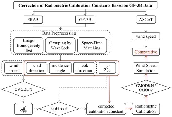
Figure 4. Flowchart for Correction of GF-3B Radiometric Calibration Constants with GMF and Wind Field Data.

Preprocessing was conducted on both GF-3B and wind field data, including homogeneity testing, data grouping, and data matching. Data grouping was performed by beam code, as the radiometric calibration constants of SAR data are correlated with satellite platform attitude parameters. For instance, according to the published radiometric calibration constants of the GF-3 satellite, data acquired from the same beam code share identical calibration constants. After space-time matching, wind speed, wind direction, incidence angle, and look direction information for each matched point were input into CMOD5.N, yielding the simulated NRCS ${\sigma }_{vv}^{0\prime }$ under the corresponding conditions. The uncalibrated NRCS from GF-3B measurements is denoted as ${\sigma }_{vv}^{0″}$. Following Equation (1), the simulated radiometric calibration constant $k_{dB}^{\prime }$ was then calculated as $k_{dB}^{\prime }={\sigma }_{vv}^{0″}$ − ${\sigma }_{vv}^{0\prime }$ representing the difference between the uncalibrated and simulated NRCS. For each beam code, all simulated calibration constants derived within that mode were subjected to statistical analysis. The statistically optimal value obtained from this analysis was subsequently adopted as the corrected calibration constants for the corresponding beam code.

Finally, the corrected calibration constants were applied to perform radiometric calibration. Subsequently, wind speed was retrieved using both the CMOD5.N and CMOD7 models. The effectiveness of the radiometric calibration correction was validated by comparing the retrieved wind speeds with ERA5 and ASCAT wind field data.

Accordingly, this study grouped 490 GF-3B images according to the beam code and inverted the radiometric calibration constants for 10 beam codes with a larger number of images, which are listed in Table 2.

Table 2. Correction Results of Radiometric Calibration Constants for VV-polarized Data in 10 beam codes of GF-3B.

Beam Code	Original Calibration Constants	Corrected Calibration Constants
189	31.52	31.43
191	31.89	30.93
192	31.89	30.87
197	31.89	31.71
200	31.89	29.62
201	37.60	30.83
202	31.89	29.59
205	31.89	35.52
212	37.25	33.44
214	36.19	33.93

Using the calibration constants before and after correction in conjunction with CMOD5.N and CMOD7, SSWS retrieval validation was performed separately with ERA5 and ASCAT wind field data. The wind speed retrieval results are presented in Figure 5 and Figure 6.

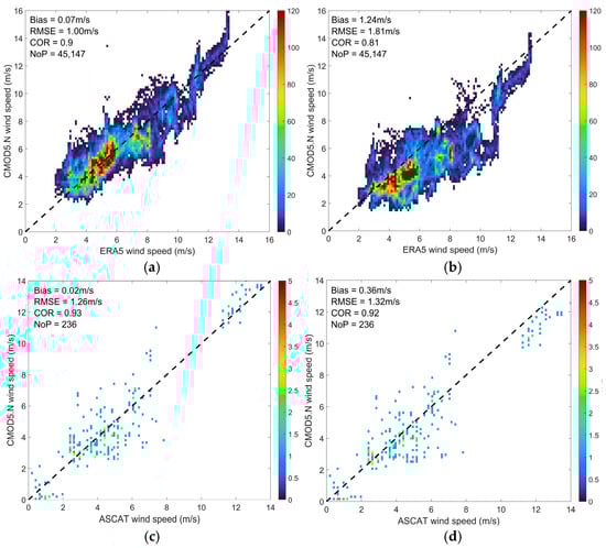
Figure 5. Comparison of SSWS Retrieval from GF-3B Using Calibration Constants Before and After Correction with the CMOD5.N. (a) Results of wind speed retrieval using the corrected calibration constants (ERA5). (b) Results of wind speed retrieval using the original calibration constants (ERA5). (c) Results of wind speed retrieval using the corrected calibration constants (ASCAT). (d) Results of wind speed retrieval using the original calibration constants (ASCAT).

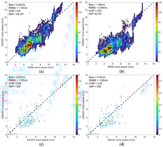
Figure 6. Comparison of SSWS Retrieval from GF-3B Using Calibration Constants Before and After Correction with the CMOD7. (a) Results of wind speed retrieval using the corrected calibration constants (ERA5). (b) Results of wind speed retrieval using the original calibration constants (ERA5). (c) Results of wind speed retrieval using the corrected calibration constants (ASCAT). (d) Results of wind speed retrieval using the original calibration constants (ASCAT).

In Figure 5, when ERA5 was used as the external wind field dataset, the bias between wind speeds retrieved with the original calibration constants and ERA5 winds was 1.24 m/s, with an RMSE of 1.81 m/s. In contrast, application of the corrected calibration constants reduced the bias to 0.07 m/s and the RMSE to 1 m/s. Figure 5a illustrates a pronounced elevation in retrieved wind speeds relative to Figure 5b, effectively eliminating the systematic underestimation observed near ERA5 winds of 10 m/s. The correlation coefficient (COR) between retrieved and ERA5 wind speeds increased from 0.81 to 0.90. When ASCAT was used as the external wind field dataset, retrievals based on the original calibration constants exhibited a bias of 0.36 m/s and an RMSE of 1.32 m/s. With the corrected calibration constants, these values improved to 0.02 m/s (bias) and 1.26 m/s (RMSE), consistent with the improvement pattern observed in the ERA5 case. Although the 236 spatio-temporal collocated points between GF-3B and ASCAT wind field data lack wind speed values in the 1–11 m/s range, relevant studies have demonstrated that ASCAT and ERA5 wind fields exhibit high consistency in offshore regions and under moderate wind speed conditions [24,33]. Furthermore, evaluation metrics indicate that the SSWS retrieved using the revised calibration constants are closer to the ASCAT wind speeds. This improvement is particularly evident when ASCAT wind speeds reach 12 m/s, where the CMOD5.N retrieved winds show a marked increase. As shown in Figure 6, retrievals from the CMOD7 and CMOD5.N models exhibited favorable consistency. More importantly, by applying the corrected calibration constants, the accuracy of SSWS retrieval was significantly improved, with the RMSE reduced by approximately 44% compared to ERA5 wind field data.

To conclude, SSWS retrievals from GF-3B data using CMOD models with corrected calibration constants show good agreement with both ERA5 and ASCAT wind fields. These findings demonstrate that the radiometric calibration constant correction method proposed in this study effectively improves the calibration accuracy of GF-3B satellite data and meets the requirements for SSWS retrieval.

4. An Attention-Guided Dual-Branch Feature-Fusion Neural Network for SSWS Retrieval

Based on the corrected calibration constants, this study investigates SSWS retrieval methods using GF-3 series SAR satellite data. To fully exploit the spatial features of sea surface wind fields embedded in SAR image while emphasizing fine-scale characteristics, an attention-guided dual-branch feature-fusion neural network is developed for SSWS retrieval. The proposed model employs a dual-branch architecture to extract both spatial features and nonlinear relationships from multimodal inputs, with feature fusion facilitated through a channel attention mechanism.

4.1. Proposed Network Model

SSWS was retrieved using the proposed ADBFF-NET, with GF-3 VV-polarized data and external wind field data serving as model inputs. The GF-3B VV-polarized data were radiometrically calibrated using the corrected calibration constants derived in the preceding sections. The network adopts a dual-branch architecture that integrates a BP network with a deep residual convolutional neural network, thereby combining the BP network’s capability for nonlinear mapping with the CNN’s strength in spatial feature extraction. Multi-channel sub-images, composed of NRCS, wind direction, incidence angle, and look direction, are utilized as inputs to retrieve wind speed at the central pixel of each sub-image. The detailed architecture of the model is presented in Figure 7.

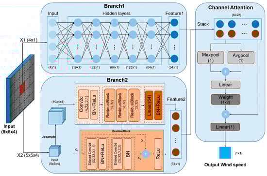
Figure 7. An Attention-Guided Dual-Branch Feature-Fusion Neural Network (ADBFF-NET).

Branch1 and Branch2 constitute two parallel feature extraction sub-modules within the network architecture. Branch1 processes a one-dimensional vector composed of central-pixel values from each channel of the multi-channel sub-image, constructing nonlinear mappings through multiple fully connected layers. In parallel, Branch2 takes the entire multi-channel sub-image as input, employing two-dimensional convolutional layers and residual blocks to extract and preserve contextual features surrounding the central pixel, thereby enhancing global-local associations. Subsequent fully connected layers in Branch2 ensure that its output features have identical dimensionality to those of Branch1. Following feature extraction, the outputs of both branches are fused, and an attention mechanism dynamically reweights the fused features to improve integration accuracy. The final fused representation is then used to retrieve wind speed at the central pixel of the sub-image. Model performance is validated against ASCAT and ERA5 wind field products. The configurations of the three critical modules (Branch1, Branch2, and the attention module) are detailed below.

• Branch1: Fully Connected Module Branch

Branch1 adopts a five-layer chain-structured architecture to extract intrinsic statistical patterns through progressive nonlinear transformations. The input is first projected into a 16-dimensional feature space through a linear layer, then expanded sequentially to 32, 64, and 128 dimensions before being reduced to 64 dimensions. The design integrates Batch Normalization (BatchNorm) and Dropout for complementary optimization: Dropout is applied after ReLU activations in the first two layers to mitigate feature co-adaptation, while BatchNorm in the subsequent three layers stabilizes gradient propagation. The 128-dimensional intermediate layer notably enhances the expressive capacity for high-order nonlinear features. A primary limitation of this branch is its limited sensitivity to local spatial patterns, necessitating complementary features from the convolutional branch.

2.

Branch2: Residual Module Branch

Branch2 focuses on extracting multi-scale spatial features from four-channel 5 × 5 local regions, integrating dilated convolutions with residual connections. Inputs are upsampled to 10 × 10 via bilinear interpolation, followed by a 3 × 3 convolution and BatchNorm to capture fundamental spatial patterns. The core processing unit comprises a cascade of three enhanced residual modules (Residual Block in Figure 7): The first layer in each module employs a standard 3 × 3 convolution (dilation = 1, padding = 1) to capture local details, while the second layer uses a dilated 3 × 3 convolution (dilation = 2, padding = 2) to expand the receptive field; stacking across modules further enhances the receptive field hierarchically. Residual skip connections preserve original feature information via identity mapping and shorten gradient paths, thereby mitigating vanishing gradients. After feature extraction, spatial features are flattened, compressed to a 64-dimensional representation via a fully connected layer, and further regularized with BatchNorm and Dropout to improve generalization. This branch enables dynamic multi-scale perception on feature maps, providing spatial features for SSWS inversion.

3.

Channel Attention Mechanism Module

To fuse the nonlinear mapping features and spatial features produced by the parallel network, a Channel Attention Mechanism (CAM) is employed for adaptive weighting and feature integration. The corresponding network architecture is illustrated in Figure 8.

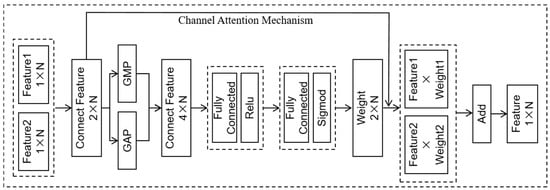
Figure 8. Channel Attention Mechanism for Feature Fusion.

The feature-fusion workflow using the channel attention mechanism proceeds as follows. First, the two input features, Feature1 and Feature2, are concatenated along the channel dimension. Next, both global average pooling (GAP) and global max pooling (GMP) are applied to this concatenated feature to generate two distinct sets of channel-wise statistics. These statistics are subsequently concatenated and passed through two fully connected (FC) layers, with a ReLU activation function between them, to obtain transformed representations. A sigmoid activation function is then applied to produce a set of normalized channel attention weights. Finally, these weights are used to recalibrate the original Feature1 and Feature2 via channel-wise multiplication, and the weighted features are summed to produce the final fused output. The mathematical formulation for weight generation and fusion is provided in Equation (4).

$$\left\{\begin{array}{c}\mathrm{W}=\mathrm{S}\mathrm{i}\mathrm{g}\mathrm{m}\mathrm{o}\mathrm{d}\left({\mathsf{\omega }}_2\times \mathrm{R}\mathrm{e}\mathrm{l}\mathrm{u}\left({\mathsf{\omega }}_1\times \left[\mathrm{G}\mathrm{A}\mathrm{P}\left({\mathrm{F}}_{\mathrm{c}\mathrm{o}\mathrm{n}\mathrm{n}\mathrm{e}\mathrm{c}\mathrm{t}}\right),\mathrm{G}\mathrm{M}\mathrm{P}\left({\mathrm{F}}_{\mathrm{c}\mathrm{o}\mathrm{n}\mathrm{n}\mathrm{e}\mathrm{c}\mathrm{t}}\right)\right]\right)\right)\\ {\mathrm{F}}_{\mathrm{f}\mathrm{u}\mathrm{s}\mathrm{e}\mathrm{d}}={\mathrm{W}}_1\times {\mathrm{F}}_1+{\mathrm{W}}_2\times {\mathrm{F}}_2\end{array}\right.$$

(4)

where ${\mathsf{\omega }}_1$ and ${\mathsf{\omega }}_2$ denote the weights of the fully connected layers, ${\mathrm{W}}_1$ and ${\mathrm{W}}_2$ indicate the attention weights assigned to features Feature1 and Feature2, and ${\mathrm{F}}_1$ and ${\mathrm{F}}_2$ correspond to the original features Feature1 and Feature2.

4.2. Sample Preparation and Model Training

The sample preparation workflow adopted in this study is illustrated in Figure 9, where the spatial matching method for SAR data and wind field data employs Method 1. First, space-time matching was performed between SAR data and wind field data. Then, a 5 × 5 sliding window was applied along both rows and columns to extract sub-image patches of size 5 × 5 × 4. Each patches comprise four channels: ${\mathsf{\sigma }}_{\mathrm{v}\mathrm{v}}^0$, $\mathsf{\theta }$, $\cos \left(\mathrm{\varnothing }\right)$, and $\cos \left(2\mathrm{\varnothing }\right)$ [16]. To enhance training efficiency and improve generalization and robustness, channel-wise normalization was conducted based on the empirical numerical distributions of each feature channel.

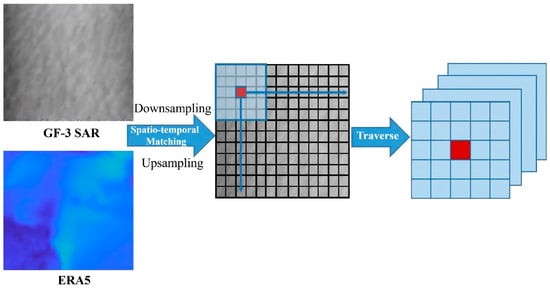
Figure 9. SAR Sample Preparation Workflow Diagram.

A total of 2607 SAR images were spatiotemporally matched with the ERA5 and ASCAT wind field datasets. 2553 images were successfully matched with ERA5, whereas only 442 images were matched with ASCAT. To ensure independence among the training, validation, and test sets, the matched SAR images were randomly partitioned into these three subsets prior to sample preparation. The final partitions of the matched SAR data are summarized in Table 3.

Table 3. Statistical Table of Dataset Partitioning for SAR-ERA5 and SAR-ASCAT.

	SAR-ERA5 Matched Images	SAR-ASCAT Matched Images
Training Set	1536	255
Validation Set	508	84
Test Set	509	83
Total	2553	442

Using the above methodology, sample preparation was conducted on 1536 SAR images from the SAR-ERA5 training set and 255 SAR images from the SAR-ASCAT training set, yielding 62,537 and 24,765 samples, respectively. The wind speed distributions of these datasets, shown as gray histograms in Figure 10a,b, exhibit pronounced non-uniformity. To improve suitability for model training, data cleaning was performed by adjusting sample counts across wind speed bins. A normal distribution curve (mean = 8, variance = 5) is plotted as a red dashed line in Figure 10a,b. For bins where the sample count exceeded the normal curve, samples were randomly reduced; conversely, for bins below the curve, data augmentation was applied by rotating sub-image patches to increase sample numbers. Note that the 3D sub-image patch must be rotated as a whole to preserve the physical relationships among ${\mathsf{\sigma }}_{\mathrm{v}\mathrm{v}}^0$, $\mathsf{\theta }$, $\cos \left(\mathrm{\varnothing }\right)$, and $\cos \left(2\mathrm{\varnothing }\right)$. No augmentation was performed for wind speeds below 2 m/s due to known ERA5 inaccuracy in this range. After cleaning, the SAR-ERA5 and SAR-ASCAT training sets contained 56,917 and 22,555 usable samples, respectively, with blue histograms in Figure 10a,b illustrating the resulting distributions. The same cleaning procedure was applied synchronously to the validation sets of both datasets. Final sample counts used for model training are summarized in Table 4.

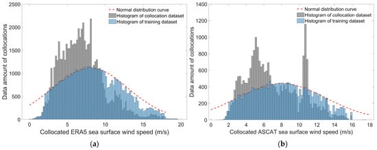
Figure 10. Histogram of wind speed distribution for the training sets in both SAR-ERA5 and SAR-ASCAT datasets. (a) Histogram of wind speed distribution for the SAR-ERA5 training set. (b) Histogram of wind speed distribution for the SAR-ASCAT training set.

Table 4. Detailed Information on the SAR-ERA5 and SAR-ASCAT Datasets.

	SAR-ERA5	SAR-ASCAT
Training Set	56,917	22,555
Validation Set	23,343	7765
Test Set	20,948	6916
Total	101,208	37,236

In order to leverage the complementarity of multi-source wind field data to constrain the model and reduce the systematic bias inherent in any single data source, ADBFF-NET was trained using a merged dataset combining both SAR-ERA5 and SAR-ASCAT data. To improve convergence efficiency, a second-order optimization strategy was adopted during training. The primary optimizer was AdamW (learning rate = 0.001, weight decay = 1 × 10⁻⁴), complemented by a dynamic learning rate scheduler and gradient clipping to monitor validation loss and prevent gradient explosion. The conventional MSE loss function tends to disproportionately amplify errors from high-error samples due to the squaring effect, which causes the model to overemphasize accuracy in the medium-to-high wind speed ranges while underrepresenting the low-wind-speed regions where absolute errors are inherently smaller. To address this issue, a wind-speed-weighted loss function was introduced. By assigning appropriate weights to different wind speed intervals, this function ensures that losses across all ranges are adequately considered during training. The formulation of the weighted loss function is given in Equation (5).

$$\mathrm{l}\mathrm{o}\mathrm{s}\mathrm{s}={\displaystyle \frac{1}{\mathrm{N}}}\left(\sum _{\mathrm{i}=1}^{\mathrm{N}}{\mathrm{w}}_{\mathrm{i}}{\left({\mathrm{y}}_{\mathrm{i}}-{\widehat{\mathrm{y}}}_{\mathrm{i}}\right)}^2\right)$$

(5)

where N is the number of samples in the batch; i is the sample index; ${\mathrm{y}}_{\mathrm{i}}$ is the true value of the i-th sample; ${\widehat{\mathrm{y}}}_{\mathrm{i}}$ is the model-predicted value of the i-th sample; ${\mathrm{w}}_{\mathrm{i}}$ is the weight of the i-th sample. After iterative experimental adjustments, the weight configurations for the merged dataset are [6, 2, 1.5, 1.8], with corresponding wind speed intervals of [0 m/s, 3 m/s, 6 m/s, 14 m/s, 20 m/s].

4.3. Experimental Verification

4.3.1. Experiment Based on ERA5 and ASCAT Wind Field Data

After the model training was completed, SSWS retrieval was performed on the 20,948 SAR-ERA5 and 6916 SAR-ASCAT test set samples detailed in Table 4 using both the ADBFF-NET and CMOD5.N models. The results are presented in Figure 11.

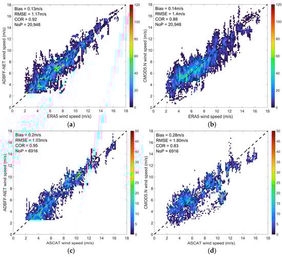
Figure 11. Comparison of Wind Speed Retrieval Results between ADBFF-NET and CMOD5.N. (a) Retrieved wind speeds from the proposed model (ERA5). (b) Retrieved wind speeds from CMOD5.N (ERA5). (c) Retrieved wind speeds from the proposed model (ASCAT). (d) Retrieved wind speeds from theCMOD5.N (ASCAT).

As shown in Figure 11a,b, the performance of the ADBFF-NET model on the SAR-ERA5 test set is markedly superior to that of CMOD5.N. In terms of key statistical metrics, the RMSE between the ADBFF-NET retrieved wind speeds and the ERA5 winds speed is 1.17 m/s, representing a reduction of approximately 16% compared to CMOD5.N. The bias of ADBFF-NET is 0.13 m/s, which is comparable to that of CMOD5.N, while the COR increases from 0.88 to 0.92, indicating better consistency between the ADBFF-NET retrievals and the ERA5 reference data. Analysis of the scatter plots in Figure 11a,b shows that the performance improvement of the ADBFF-NET model is most evident in two wind speed ranges. In the low-speed regime (approximately 2–6 m/s), the CMOD5.N retrievals are systematically located above the 1:1 reference line, indicating an overestimation bias in this range. In contrast, the ADBFF-NET retrievals are distributed symmetrically around the reference line, effectively correcting this systematic bias. For wind speeds above 8 m/s, the ADBFF-NET retrievals form a tighter and more concentrated cluster along the reference line, significantly reducing the dispersion compared to CMOD5.N.

For the SAR-ASCAT test set, although the model was trained with a significantly larger number of SAR-ERA5 samples than SAR-ASCAT samples, which may introduce a data source bias, Figure 11c,d clearly show that the ADBFF-NET model also achieves a significant improvement over CMOD5.N. Compared against ASCAT wind speeds, the RMSE of the ADBFF-NET retrievals is 1.03 m/s, which is 0.77 m/s lower than that of CMOD5.N. The bias of ADBFF-NET is 0.2 m/s, slightly lower than that of CMOD5.N, while the COR increases markedly from 0.83 to 0.95, indicating that the ADBFF-NET retrievals also maintain good consistency with the ASCAT measurements. In terms of scatter plot distribution, CMOD5.N exhibits a clear systematic overestimation in the low wind speed regime (<6 m/s), with its high-density point cloud deviating upward from the reference line. In contrast, the ADBFF-NET retrievals show a more symmetric distribution along the reference line in this region. Furthermore, across the entire wind speed range, and particularly at high wind speeds, the dispersion of the ADBFF-NET retrievals is lower than that of CMOD5.N. These results demonstrate that the features learned by the model from multi-source data possess a considerable degree of robustness and generalization capability.

In summary, the ADBFF-NET model demonstrates robust wind speed retrieval performance on both independent test sets. Improvements across all key statistical metrics compared to CMOD5.N confirm its higher retrieval accuracy and stronger consistency with the reference wind field data. Notably, although SAR-ERA5 samples outnumbered SAR-ASCAT samples during the training phase, the model still achieved a clear performance gain on the SAR-ASCAT test set. This highlights that the proposed deep learning framework, through feature learning, can effectively mitigate the potential impact of training data imbalance and possesses sound generalization capability.

4.3.2. Comparison Between Retrieved Wind Speeds and Altimeter-Derived Wind Speeds

To validate the performance of the ADBFF-NET model, trained on SAR-ERA5 and SAR-ASCAT sample data, for high-resolution SAR SSWS retrieval, this study performed spatiotemporal matching between the test set sample data and the near-real-time along-track SWH products. The spatiotemporal matching procedure is described in Section 2.5.3, and the spatial matching method employed was Method 2. A total of 209 SAR-altimeter wind speed match-ups were obtained. Wind speed retrieval was performed using both the ADBFF-NET model and the CMOD5.N model, followed by a comparative analysis with the altimeter wind speeds and ERA5 wind speeds.

Figure 12 presents a comparative analysis of wind speeds retrieved by the proposed ADBFF-NET model and the traditional CMOD5.N model against independent reference data from altimeters and ERA5 reanalysis across 209 locations. As shown in Figure 12a, the bias between the wind speeds retrieved by ADBFF-NET and the altimeter measurements is 0.16 m/s, representing a reduction of approximately 78% compared to CMOD5.N. The RMSE is 2.10 m/s, and the COR is 0.63, which is comparable to that of CMOD5.N. This indicates that ADBFF-NET achieves superior bias control, though its correlation with the altimeter winds shows a slight decrease. The scatter plot distribution reveals a certain degree of dispersion between the retrieval results of both models and the altimeter data, with the dispersion increasing notably when wind speeds exceed 8 m/s. This suggests that although the ADBFF-NET model is built upon deep learning, its retrieval accuracy and generalization capability face challenges when applied to high-resolution, independent wind field data, which exhibits a significant scale difference from the training data (0.25° resolution). Overall, its performance remains comparable to the long-operational CMOD5.N model. In contrast, the ADBFF-NET retrievals show better consistency with ERA5 wind speeds, as illustrated in Figure 12c. The bias is 0.08 m/s, the RMSE is 1.70 m/s, and the COR is 0.76. All metrics show improvement compared to the retrieval results of the CMOD5.N model. This fully confirms that ADBFF-NET can effectively learn and fit the statistical characteristics and physical relationships contained within its training data.

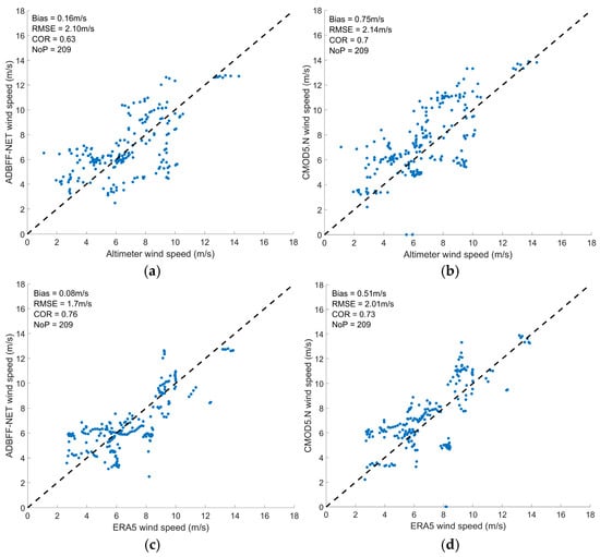
Figure 12. Comparative analysis of retrieved versus altimeter wind speeds. (a) Comparison of ADBFF-NET Retrieved Wind Speed with Altimeter Measurements. (b) Comparison of CMOD5.N Retrieved Wind Speed with Altimeter Measurements. (c) Comparison of ADBFF-NET Retrieved Wind Speed with ERA5 Reanalysis Data. (d) Comparison of CMOD5.N Retrieved Wind Speed with ERA5 Reanalysis Data.

The analysis above indicates that the performance of the proposed model depends on the consistency between the validation data and the training data. When there is a significant difference in spatial resolution between the test data and the training data, the advantages of the model are not fully realized, and its retrieval performance is comparable to that of the CMOD5.N model. This reveals the current model’s limitation in generalizing from lower-resolution training data to higher-resolution observational data. Future work should consider incorporating multi-resolution data during training or designing network architectures that target scale invariance, in order to further enhance the model’s applicability for retrieving high-resolution wind field data.

Furthermore, this study acquired three images of GF-3 FSII mode over the Taiwan Strait, imaged at 22:00 on 12 March 2023, which were then matched with AltiKa altimeter wind speeds to obtain 37 matching points. To further validate the wind speed retrieval performance of the proposed model in nearshore scenarios, the ADBFF-NET model and the CMOD5.N model were applied to retrieve wind speeds from these three images. Concurrently, the ERA5 wind field data within the region were upsampled. The results are presented in Figure 13.

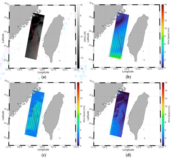
Figure 13. Wind speed retrieval from GF-3 FSII mode SAR data. (a) GF-3 SAR Backscattering Coefficient. (b) ERA5 Interpolated Wind Field Results. (c) ADBFF-NET Retrieved Wind Speed Results. (d) CMOD5.N Retrieved Wind Speed Results.

The Bias and RMSE between the retrieved wind speeds from the ADBFF-NET, CMOD5.N, and the upsampled ERA5 wind speeds against the altimeter wind speeds at the 37 collocated points were calculated, and the results are presented in Table 5.

Table 5. Comparison of Retrieved Wind Speed versus Altimeter Wind Speed.

	ADBFF-NTE Wind Speed (m/s)	CMOD5.N Wind Speed (m/s)	ERA5 Wind Speed (m/s)
Bias	0.76	2.67	0.59
RMSE	1.57	2.85	1.11

As shown in Figure 13 and Table 5, the wind speed retrieved by the CMOD5.N model is systematically lower, with a Bias of 2.67 m/s and an RMSE of 2.85 m/s, indicating substantial errors compared to both the altimeter measurements and the ERA5 wind field. This is likely because coastal areas exhibit complex sea state conditions, while the ERA5 wind field data have a spatial resolution of 0.25°, making it difficult to provide detailed sea surface wind direction information. This, in turn, affects the overall accuracy of wind speed retrieval using CMOD5.N.

In contrast, the wind speed retrieval results of the ADBFF-NET model for the 37 collocated points generally align with expectations. The Bias between its retrieved wind speeds and the altimeter wind speeds is 0.76 m/s, and the RMSE is 1.57 m/s, showing an improvement over the systematic underestimation observed with the CMOD5.N model. This is likely because the sample dataset used for training the proposed model includes some data from coastal scenarios (as shown in Figure 1), enabling the ADBFF-NET model to maintain decent performance even in nearshore environments. Notably, the interpolated ERA5 wind speeds still exhibit low bias and RMSE relative to the altimeter wind speeds, indicating good consistency between the two wind field data sources. This consistency also explains why the wind speeds retrieved by the ADBFF-NET model roughly match the altimeter measurements, laying a foundation for the model’s application in high-resolution wind speed retrieval. Although, in terms of metrics, the interpolated ERA5 wind speeds appear closer to the altimeter wind speeds than those retrieved by ADBFF-NET, Figure 13b,c reveal that ADBFF-NET more effectively preserves the fine-scale spatial structural features of the sea surface wind field. Compared to the smoothed interpolated ERA5 wind speeds, the ADBFF-NET results are closer to the actual wind field conditions.

5. Discussion

First, the radiometric calibration accuracy of VV-polarized data from the GF-3B satellite was validated using 490 fully polarimetric images. The results showed that the calibration accuracy of certain beam codes did not meet the requirements for SSWS retrieval. As shown in Figure 3, NRCS scatter points for some data fell outside ±1.31 dB. Zhang et al. [34] reported similar findings when evaluating the wind speed retrieval capability of GF-3B. Although their calibration accuracy threshold (1.43 dB) differs from the threshold adopted in this study (1.31 dB), both indicate that GF-3B NRCS deviations, when retrieved using CMOD5.N, exceed acceptable ranges. By analyzing a larger dataset, this study further demonstrates that discrepancies in GF-3B radiometric calibration accuracy increase with incidence angle. To mitigate this issue, a beam code grouping strategy was implemented to correct the radiometric calibration constants for specific GF-3B beam codes. Subsequently, ideal NRCS was simulated by combining the GMF with ERA5 wind fields, and calibration constants were adjusted according to the deviations between simulated and original NRCS. This correction enabled the use of selected beam codes from the GF-3B satellite for SSWS retrieval.

However, although the feasibility of the radiometric calibration constant correction method proposed in this study has been verified, experimental results indicate that, for GF-3 SAR data under the same beam code, even after removing interference factors such as sea ice, oil spills, and ocean fronts, the retrieved radiometric calibration constants still exhibit variations when derived from observations of different orbital passes. As shown in Figure 14, a total of 85 fully polarimetric GF-3B images with beam code 189 were analyzed, spanning several orbits, with the majority originating from orbits 7701, 7714, and 7711. Grouped by orbit, the derived calibration constants were 32.17 dB, 31.81 dB, and 30.91 dB, respectively, with a maximum divergence of 1.26 dB. The unified calibration constant derived from all 85 images was 31.43 dB, differing by only 0.09 dB from the original calibration constant. This demonstrates satisfactory radiometric accuracy for this beam code, as deviations for all three orbit-specific constants remained below 0.8 dB, meeting the precision requirements for wind speed retrieval. Nevertheless, obtaining the globally optimal calibration constant for the entire beam code necessitates large-scale data inversion via the proposed method. While limited data volume for certain beam codes may yield locally optimal solutions, the derived calibration constants remain adequate for operational wind speed retrieval applications. As for the factors causing differences in the retrieved radiometric calibration constants from data of different orbital passes under the same beam code, the variation in incidence angle may be a possible reason, but specific factors require further comprehensive analysis in subsequent work.

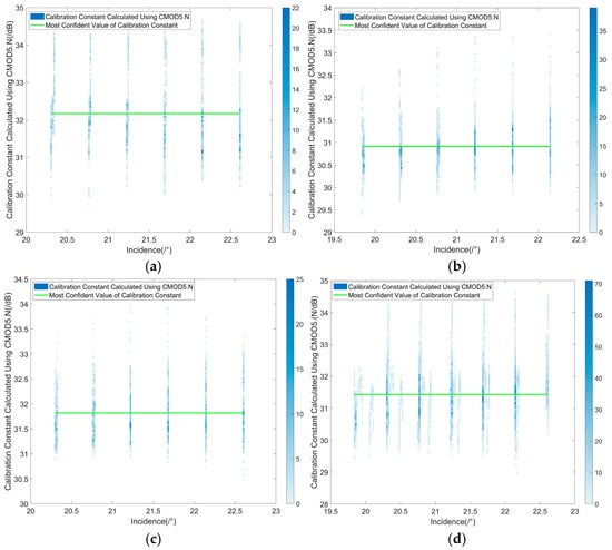
Figure 14. Retrieval Results of Radiometric Calibration Constants under Different Orbital Conditions. (a) Radiometric calibration constant retrieval for Orbit 7701 data. (b) Radiometric calibration constant retrieval for Orbit 7711 data. (c) Radiometric calibration constant retrieval for Orbit 7714 data. (d) Radiometric calibration constant retrieval for merged data.

Data characteristics of the three orbits GF-3B acquisitions in Figure 14 are summarized in Table 6.

Table 6. Retrieved calibration constants for GF-3B beam code = 189 data across four orbits.

Orbit ID	7701	7714	7711	Others	Merged
Image count	18	19	29	19	85
Optimal estimate of radiometric calibration constants retrieved using CMOD5.N model (dB)	32.17	31.81	30.91	31.10	31.43

Secondly, following the correction of radiometric calibration constants for GF-3B data, this study proposed an attention-guided dual-branch feature-fusion model for SSWS retrieval. The model leverages a BP network to establish nonlinear mapping capabilities, employs residual modules to extract local spatial features, and integrates a channel attention mechanism for feature fusion to derive SSWS. Previous studies have validated the efficacy of BP networks in SAR-based wind speed retrieval. For instance, Li et al. developed a GMF-guided BPNN model for Sentinel-1 IW-mode HH-Polarized SAR data in the Arctic marginal ice zone, achieving an RMSE of 1.25 m/s [16]. As a spatiotemporal dynamic process, the sea surface wind field inevitably influences wind speed retrieval through its two-dimensional spatial characteristics manifested in SAR imagery. Given that distinct wind speeds exhibit different features in SAR imagery, existing studies have employed machine learning and deep learning methods to extract spatial features from SAR data, performing feature optimization integrated with external wind field information to achieve wind speed retrieval [35,36,37], thereby demonstrating the role of SAR spatial features in SSWS retrieval.

The model proposed in this study adopts residual modules to mine spatial features, following this established concept. It utilizes multi-channel sub-image patches composed of radar NRCS, incidence angles, wind direction, and other relevant parameters as model inputs. However, unlike conventional approaches, this study mitigates the impact of resolution discrepancies between SAR data and external wind field data on wind speed retrieval by downsampling SAR images to 2 km resolution during data preprocessing [38]. Each sample encompasses a 10 km × 10 km region, where spatial features extracted from the sub-image area combined with the nonlinear mapping relationship at the central pixel location collectively estimate SSWS at that central pixel. This strategy further enhances wind speed estimation accuracy. Recent studies have validated the effectiveness of parallel network architectures combining residual and BP networks for inverting ocean dynamic parameters [39]. Building on this foundation, this study incorporates an attention mechanism to deeply integrate nonlinear and spatial features, which enhances the saliency of critical features while suppressing irrelevant information interference.

Based on the comparative results between the wind speeds retrieved by the ADBFF-NET model and external wind field data shown in Figure 11 and Figure 12, it is evident that for the lower spatial resolution ERA5 and ASCAT wind fields, the retrieved wind speeds from the proposed model exhibit high consistency with both ERA5 and ASCAT winds, demonstrating a significant performance improvement over CMOD5.N. However, when compared with the altimeter wind speeds with a spatial resolution of 7 km, the performance of the proposed model in wind speed retrieval is generally comparable to that of CMOD5.N. It is noteworthy that wind speed retrieval experiments conducted on 37 SAR-Altimeter collocations located in the Taiwan Strait reveal that under complex nearshore sea state conditions, where CMOD5.N performs poorly, the proposed model remains stable. Furthermore, its retrieval results preserve the fine-scale spatial structure of the sea surface wind field more effectively than the spatially interpolated ERA5 wind field. This demonstrates the potential of the ADBFF-NET model for high-resolution SSWS retrieval.

The feasibility of the proposed model for GF-3B SSWS retrieval has been validated; however, three key limitations warrant further refinement. First, the significant resolution discrepancy between external wind field products and GF-3 fully polarimetric data compromises the inherent high-resolution advantage of GF-3 observations. Second, given its derivation from balancing downsampled GF-3 data resolution against wind field product constraints, the current 5 × 5 multi-channel sub-image patch size requires optimization in future studies to quantify its impact on retrieval accuracy impacts. Third, regarding feature inputs, the current model utilizes four input channels: ${\mathsf{\sigma }}_{\mathrm{v}\mathrm{v}}^0$, $\mathsf{\theta }$, $\cos \left(\mathrm{\varnothing }\right)$, and $\cos \left(2\mathrm{\varnothing }\right)$. Future research should explore the impact of diverse feature combinations on retrieval accuracy. For instance, information such as azimuth cutoff [40] and co-cross-polarization coherence [41]; meanwhile, existing studies have validated the feasibility of SAR SSWS retrieval independent of external wind field information [42,43], offering a novel solution for high-resolution SAR SSWS inversion.

6. Conclusions

This study conducts SSWS retrieval based on fully polarimetric data from the GF-3 series satellite. First, the radiometric calibration accuracy of GF-3B data was validated, revealing that certain beam codes failed to meet international deviation requirements for wind speed retrieval. Subsequently, a correction strategy was applied by integrating the CMOD5.N with ERA5 wind field data to adjust the radiometric calibration constants for these substandard beam codes. Based on the revised constants, SSWS were retrieved using the CMOD5.N, CMOD7 and validated against ERA5 winds and ASCAT winds. The results demonstrated significant improvements: the RMSE between retrieved winds and ERA5 winds reached 1 m/s, while the RMSE against ASCAT winds was 1.26 m/s. Compared to results derived from the original calibration constants, these metrics reflect a marked enhancement in accuracy. Notably, the systematic underestimation trend observed in original retrievals relative to ERA5 winds was effectively mitigated, thereby validating the efficacy of the proposed radiometric calibration constant correction for GF-3B data.

To further improve the retrieval performance, an attention-guided dual-branch feature-fusion network was constructed to retrieve SSWS through three-dimensional sub-image patches. Experimental results demonstrate that the wind speeds retrieved by the ADBFF-NET model achieve an RMSE of 1.17 m/s and a COR of 0.92 against ERA5 winds, and an RMSE of 1.03 m/s with a COR of 0.95 against ASCAT winds. All metrics show improvement compared with the CMOD5.N model, effectively correcting the systematic overestimation by CMOD5.N in low-wind-speed regions and its systematic underestimation in high-wind-speed regions. Meanwhile, the wind speeds retrieved by the ADBFF-NET model exhibit a bias of 0.16 m/s and an RMSE of 2.10 m/s against altimeter winds, demonstrating performance largely consistent with that of the CMOD5.N model, which verifies the effectiveness of the proposed model for high-resolution SSWS retrieval. Furthermore, experiments using GF-3 FSII mode data from the Taiwan Strait show that the proposed model maintains robust wind speed retrieval performance in nearshore scenarios and can effectively preserve the fine-scale spatial features of the sea surface wind field.

In summary, the radiometric calibration constant correction method proposed in this study can effectively improve the accuracy of GF-3 SAR radiometric calibration constants, meeting the requirements for SAR SSWS retrieval. Meanwhile, for lower-resolution retrieval tasks, the proposed ADBFF-NET model significantly enhances consistency with independent scatterometer observations (ASCAT). However, when generalizing to higher-resolution independent observations (Altimeter), while it effectively preserves the spatial structural features of the sea surface wind field, no improvement in accuracy is observed.

References

- Stoffelen, A.; Anderson, D. Scatterometer data interpretation: Estimation and validation of the transfer function CMOD4. J. Geophys. Res. Ocean. 1997, 102, 5767–5780. [Google Scholar] [CrossRef]
- Hersbach, H.; Stoffelen, A.; Haan, S.D. An improved C-band scatterometer ocean geophysical model function: CMOD5. J. Geophys. Res. Ocean. 2007, 112, C03006. [Google Scholar] [CrossRef]
- Hersbach, H. Comparison of C-Band Scatterometer CMOD5.N Equivalent Neutral Winds with ECMWF. J. Atmos. Ocean. Technol. 2010, 27, 721–736. [Google Scholar] [CrossRef]
- Wan, Y.; Guo, S.; Li, L.G.; Qu, X.J.; Dai, Y.S. Data Quality Evaluation of Sentinel-1 and GF-3 SAR for Wind Field Inversion. Remote Sens. 2021, 13, 3723. [Google Scholar] [CrossRef]
- Wang, H.; Yang, J.S.; Mouche, A.; Shao, W.Z.; Zhu, J.H.; Ren, L.; Xie, C.H. GF-3 SAR Ocean Wind Retrieval: The First View and Preliminary Assessment. Remote Sens. 2017, 9, 694. [Google Scholar] [CrossRef]
- Stoffelen, A.; Verspeek, J.A.; Vogelzang, J.; Verhofe, A. The CMOD7 Geophysical Model Function for ASCAT and ERS Wind Retrievals. IEEE J. Sel. Top. Appl. Earth Obs. Remote Sens. 2017, 10, 2123–2134. [Google Scholar] [CrossRef]
- Stoffelen, A.; Aaboe, S.; Calvet, J.C.; Cotton, J.; Chiara, G.D.; Saldaña, J.F. Scientific Developments and the EPS-SG Scatterometer. IEEE J. Sel. Top. Appl. Earth Obs. Remote Sens. 2017, 10, 2086–2097. [Google Scholar] [CrossRef]
- Lu, Y.R.; Zhang, B.; Perrie, W.; Mouche, A.; Zhang, G.S. CMODH Validation for C-Band Synthetic Aperture Radar HH Polarization Wind Retrieval Over the Ocean. IEEE Geosci. Remote Sens. Lett. 2021, 18, 102–106. [Google Scholar] [CrossRef]
- Fan, K.G.; Xu, Q.; Xu, D.Y.; Xie, H.R.; Ning, J.; Huang, J.G. Review of remote sensing of sea surface wind field by space-borne SAR. Prog. Geophys. 2022, 37, 1807–1817. [Google Scholar]
- Mouche, A.; Chapron, B.; Knaff, J.; Zhao, Y.L.; Zhang, B.; Combot, C. Co-polarized and Cross-Polarized SAR Measurements for High-Resolution Description of Major Hurricane Wind Structures: Application to Irma Category 5 Hurricane. J. Geophys. Res. Ocean. 2019, 124, 3905–3922. [Google Scholar] [CrossRef]
- Hauser, D.; Abdalla, S.; Ardhuin, F.; Bidlot, J.R.; Bourassa, M.; Cotton, D.; Gommenginger, C.; Evers-King, H.; Johnsen, H.; Knaff, J.; et al. Satellite Remote Sensing of Surface Winds, Waves, and Currents: Where are we Now? Surv. Geophys. 2023, 44, 1357–1446, Correction in Surv. Geophys. 2023, 44, 1447–1448. https://doi.org/10.1007/s10712-023-09786-9. [Google Scholar] [CrossRef]
- Thiria, S.; Mejia, C.; Badran, F.; Crepon, M. A neural network approach for modeling nonlinear transfer functions: Application for wind retrieval from spaceborne scatterometer data. J. Geophys. Res. Ocean. 1993, 98, 22827–22841. [Google Scholar] [CrossRef]
- Kasilingam, D.; Lin, I.I.; Khoo, V.; Hock, L. A neural network-based model for estimating the wind vector using ERS scatterometer data. In Proceedings of the 1997 IEEE International Geoscience and Remote Sensing (IGARSS), Singapore, 3–8 August 1997; Volume 4, pp. 1850–1852. [Google Scholar]
- Chen, K.S.; Tzeng, Y.C.; Chen, P.C. Retrieval of ocean winds from satellite scatterometer by a neural network. IEEE Trans. Geosci. Remote Sens. 1999, 37, 247–256. [Google Scholar] [CrossRef]
- Horstmann, J.; Schiller, H.; Schulz-Stellenfleth, J.; Lehner, S. Global wind speed retrieval from SAR. IEEE Trans. Geosci. Remote Sens. 2003, 41, 2277–2286. [Google Scholar] [CrossRef]
- Li, X.M.; Qin, T.; Wu, K. Retrieval of Sea Surface Wind Speed from Spaceborne SAR over the Arctic Marginal Ice Zone with a Neural Network. Remote Sens. 2020, 12, 3291. [Google Scholar] [CrossRef]
- Ni, H.Y.; Dong, C.M.; Liu, Z.B.; Yang, J.S.; Li, X.H.; Ren, L. Calibration of Sentinel-1 SAR retrieved wind speed based on BP neural network model. J. Mar. Sci. 2024, 42, 75–87. [Google Scholar]
- Xue, S.H.; Meng, L.S.; Geng, X.P.; Sun, H.Y.; Edwing, D.; Yan, X.H. Retrieving Ocean Surface Winds and Waves from Augmented Dual-Polarization Sentinel-1 SAR Data Using Deep Convolutional Residual Networks. Atmosphere 2023, 14, 1272. [Google Scholar] [CrossRef]
- Li, X.H.; Yan, Q.H.; Fan, C.Q.; Zhang, J. Deep learning-based sea surface wind speed retrieval method for Sentinel-1 dual-polarimetric SAR under typhoon sea state. Chin. J. Radio Sci. 2024, 39, 1095–1101. [Google Scholar]
- Guo, C.G.; Ai, W.H.; Zhang, X.; Guan, Y.N.; Liu, Y.; Hu, S.S. Correction of Sea Surface Wind Speed Based on SAR Rainfall Grade Classification Using Convolutional Neural Network. IEEE J. Sel. Top. Appl. Earth Obs. Remote Sens. 2023, 16, 321–328. [Google Scholar] [CrossRef]
- Shao, W.Z.; Zhou, Y.H.; Zhang, Q.J.; Jiang, X.W. Machine Learning-Based Wind Direction Retrieval from Quad-Polarized Gaofen-3 SAR Images. IEEE J. Sel. Top. Appl. Earth Obs. Remote Sens. 2024, 17, 808–816. [Google Scholar] [CrossRef]
- Ren, L.; Yang, J.S.; Mouche, A.; Wang, H.; Zhang, G.; Wang, J. Assessments of Ocean Wind Retrieval Schemes Used for Chinese Gaofen-3 Synthetic Aperture Radar Co-Polarized Data. IEEE Trans. Geosci. Remote Sens. 2019, 57, 7075–7085. [Google Scholar] [CrossRef]
- King, G.P.; Portabella, M.; Lin, W.M.; Stoffelen, A. Correlating Extremes in Wind Divergence with Extremes in Rain over the Tropical Atlantic. Remote Sens. 2022, 14, 1147. [Google Scholar] [CrossRef]
- Rubio, H.; Hatfield, D.; Hasager, C.B.; Kühn, M.; Gottschall, J. Ship-based lidar measurements for validating ASCAT-derived and ERA5 offshore wind profiles. Atmos. Meas. Tech. 2025, 18, 4949–4968. [Google Scholar] [CrossRef]
- Alonso-De-Linaje, N.G.; Hahmann, A.N.; Karagali, L.; Dimitriadou, K.; Badger, M. Improving the Modeled Variability Estimates of Offshore Winds in Northern Europe by Nudging ASCAT-Derived Winds. J. Appl. Meteorol. Climatol. 2024, 63, 821–836. [Google Scholar] [CrossRef]
- Hatfield, D.; Hasager, C.B.; Karagali, L. Vertical extrapolation of Advanced Scatterometer (ASCAT) ocean surface winds using machine-learning techniques. Wind Energy Sci. 2023, 8, 621–637. [Google Scholar] [CrossRef]
- Lucrezia, R.; Andrew, M. Intercalibration of ASCAT Scatterometer Winds from MetOp-A, -B, and -C, for a Stable Climate Data Record. Remote Sens. 2021, 13, 3678. [Google Scholar]
- Wang, Z.X.; Stoffelen, A.; Zou, J.H.; Lin, W.M.; Verhoef, A.; Zhang, Y. Validation of New Sea Surface Wind Products from Scatterometers Onboard the HY-2B and MetOp-C Satellites. IEEE Trans. Geosci. Remote Sens. 2020, 58, 4387–4394. [Google Scholar] [CrossRef]
- Calafat, F.M.; Cipollini, P.; Bouffard, J.; Anaith, H.; Féménias, P. Evaluation of new CryoSat-2 products over the ocean. Remote Sens. Environ. 2017, 191, 131–144. [Google Scholar] [CrossRef]
- Zieger, S.; Vinoth, J.; Young, I.R. Joint Calibration of Multiplatform Altimeter Measurements of Wind Speed and Wave Height over the Past 20 Years. J. Atmos. Ocean. Technol. 2009, 26, 2549–2564. [Google Scholar] [CrossRef]
- Zhang, T.Y.; Li, X.M.; Feng, Q.; Ren, Y.Z.; Shi, Y.N. Retrieval of Sea Surface Wind Speeds from Gaofen-3 Full Polarimetric Data. Remote Sens. 2019, 11, 813. [Google Scholar] [CrossRef]
- Wang, H.; Li, H.M.; Lin, M.S.; Zhu, J.H.; Wang, J.; Li, W.W. Calibration of the Copolarized Backscattering Measurements from Gaofen-3 Synthetic Aperture Radar Wave Mode Imagery. IEEE J. Sel. Top. Appl. Earth Obs. Remote Sens. 2019, 12, 1748–1762. [Google Scholar] [CrossRef]
- Yong, I.R.; Kirezci, E.; Ribal, A. The Global Wind Resource Observed by Scatterometer. Remote Sens. 2020, 12, 2920. [Google Scholar] [CrossRef]
- Zhang, K.; Hu, Y.X.; Yang, J.X.; Wang, X.C. Sea Surface Wind Speed Retrieval Using Gaofen-3-02 SAR Full Polarization Data. Remote Sens. 2025, 17, 591. [Google Scholar] [CrossRef]
- Jafari, Z.; Bobby, P.; Karami, E.; Taylor, R. A Novel Method for the Estimation of Sea Surface Wind Speed from SAR Imagery. J. Mar. Sci. Eng. 2024, 12, 1881. [Google Scholar] [CrossRef]
- Zhou, L.Z.; Zheng, G.; Yang, J.S.; Li, X.X.; Zhang, B.; Wang, H. Sea Surface Wind Speed Retrieval from Textures in Synthetic Aperture Radar Imagery. IEEE Trans. Geosci. Remote Sens. 2022, 60, 4200911. [Google Scholar] [CrossRef]
- Yan, Q.H.; Fan, C.Q.; Zhao, X.T.; Zhang, J. Intelligent retrieval of sea surface wind fields in the typhoon area of the Northwest Pacific Ocean from dual-polarization SAR data. Tsinghua Sci. Technol. 2025, 65, 1090–1101. [Google Scholar]
- Yu, P.; Xu, W.X.; Zhong, X.J.; Johannessen, J.A.; Yan, X.H.; Geng, X.P.; He, Y.R.; Lu, W.F. A Neural Network Method for Retrieving Sea Surface Wind Speed for C-Band SAR. Remote Sens. 2022, 14, 2269. [Google Scholar] [CrossRef]
- Wang, H.; Yang, J.S.; Lin, M.S.; Li, W.W.; Zhu, J.H.; Ren, L.; Cui, L.M. Quad-polarimetric SAR sea state retrieval algorithm from Chinese Gaofen-3 wave mode imagettes via deep learning. Remote Sens. Environ. 2022, 273, 112969. [Google Scholar] [CrossRef]
- Zhu, Y.T.; Grieco, G.; Lin, J.R.; Portabella, M.; Wang, X.Q. On the Use of Azimuth Cutoff for Sea Surface Wind Speed Retrieval From SAR. IEEE J. Sel. Top. Appl. Earth Obs. Remote Sens. 2024, 17, 10367–10379. [Google Scholar] [CrossRef]
- Longepe, N.; Mouche, A.A.; Ferro-Famil, L.; Husson, R. Co-Cross-Polarization Coherence Over the Sea Surface from Sentinel-1 SAR Data: Perspectives for Mission Calibration and Wind Field Retrieval. IEEE Trans. Geosci. Remote Sens. 2022, 60, 4200816. [Google Scholar] [CrossRef]
- Li, H.M.; Bertrand, C.; Alexis, M.; Wang, C.; Lin, W.M.; He, Y.J. Ocean surface wind wave signatures in single look complex SAR data. IEEE Trans. Geosci. Remote Sens. 2025, 63, 4203111. [Google Scholar] [CrossRef]
- Wei, X.N.; Chong, J.S.; Zhao, Y.W.; Diao, L.J.; Jin, X. Wind Field Retrieval from Co-Polarized SAR Imagery Without External Wind Direction Assistance. IEEE J. Sel. Top. Appl. Earth Obs. Remote Sens. 2025, 18, 4979–4991. [Google Scholar] [CrossRef]
Disclaimer/Publisher’s Note: The statements, opinions and data contained in all publications are solely those of the individual author(s) and contributor(s) and not of MDPI and/or the editor(s). MDPI and/or the editor(s) disclaim responsibility for any injury to people or property resulting from any ideas, methods, instructions or products referred to in the content. |
© 2026 by the authors. Licensee MDPI, Basel, Switzerland. This article is an open access article distributed under the terms and conditions of the Creative Commons Attribution (CC BY) license.