


Highlights
What are the main findings?
- Based on one year of continuous Mie-scattering lidar observations in Jinhua, three distinct typical aerosol layer structure types (single-layer concave, single-layer convex, multi-layer) are identified via K-means clustering.
- Dominant meteorological driving factors regulating the three aerosol layer structure types are quantified across four diurnal boundary-layer stages using the Boruta-random forest framework, revealing their stage-specific regulatory characteristics.
What are the implications of the main findings?
- Clarifying the aerosol layer structure types facilitates the refined extraction of aerosol layers from lidar profiles.
- The simulation of the aerosol vertical distributions needs to be combined with meteorological driving factors.
Abstract
The vertical distribution of atmospheric aerosol layers plays a fundamental role in understanding their climatic and environmental effects. Using one year of lidar observations in Jinhua, together with ground-based meteorological measurements and ERA5 reanalysis data, this study develops an integrated analytical framework to investigate the structural characteristics of aerosol layers in Mie-scattering profiles and their meteorological driving factors. K-means clustering identifies three representative aerosol layer structure types: single-layer concave, single-layer convex, and multi-layer profiles. By combining the Boruta algorithm with a random forest model, the dominant meteorological factors associated with each structure type are quantified across four boundary-layer stages (00–06, 06–12, 12–18, 18–24 LT). Temperature, humidity, wind speed, wind direction, divergence, and vertical velocity exhibit distinct influences across different boundary-layer conditions, revealing differentiated regulatory mechanisms governing aerosol layer structure change. The proposed framework establishes a coupled perspective between atmospheric dynamic/thermodynamic processes and aerosol layer structure formation, providing a basis for refined modeling of aerosol evolution and improved understanding of aerosol–meteorology interactions.
1. Introduction
Studying the vertical structure of atmospheric aerosols is essential for understanding their climatic, environmental, and health impacts. Aerosols directly modify the Earth’s radiation budget through scattering and absorption of solar radiation, and indirectly influence climate by serving as cloud condensation nuclei that regulate cloud formation and precipitation processes [1,2,3]. Accurate characterization of their vertical distribution is therefore fundamental for evaluating radiative forcing and aerosol–cloud interactions. In addition, aerosols strongly affect visibility, air quality, and human health; elevated aerosol loading is associated with reduced visibility and increased risks of respiratory and cardiovascular diseases [4,5,6,7]. Understanding the vertical distribution of aerosols thus provides a scientific basis for predicting pollution events and supporting environmental protection and public health management.
Changes in aerosol vertical structure are closely related to meteorological and environmental conditions, making it crucial to investigate their coupled interaction mechanisms. Lidar observations offer a powerful tool for this purpose, providing high-resolution vertical profiling of aerosols and enabling the differentiation of aerosol types such as dust, smoke, and anthropogenic pollutants through polarization and multi-wavelength measurements [8,9,10]. By emitting laser pulses and analyzing backscattered signals, lidar retrieves key aerosol optical parameters, including extinction and backscatter coefficients and depolarization ratios, which support a detailed characterization of aerosol concentration, type, and vertical layering [11,12,13]. For example, depolarization ratios distinguish spherical from non-spherical particles and are widely used to identify dust aerosols [14], while multi-wavelength Raman lidar further enhances aerosol type discrimination and optical property retrieval [10,15]. Doppler lidar provides complementary information on vertical wind speeds, and, when combined with Raman lidar measurements, enables the estimation of turbulent aerosol fluxes, offering valuable insights into aerosol transport and mixing processes [16,17].
Meteorological conditions exert strong control over the vertical distribution of aerosols. Boundary-layer height determines the mixing depth and constrains the vertical extent of near-surface aerosol dispersion [18,19,20]. Machine-learning-based clustering studies in northern China have shown that clean and polluted conditions exhibit markedly different vertical aerosol structures during autumn and winter, highlighting the sensitivity of aerosol layering to boundary-layer dynamics [12]. In addition, meteorological factors, including temperature, humidity, wind speed, and precipitation, indirectly shape vertical structures by modulating aerosol formation, hygroscopic growth, transport, and removal processes [21,22]. For instance, wind speed influences horizontal advection and entrainment at layer interfaces, while precipitation efficiently removes particles through wet deposition [6,23].
Environmental factors, such as anthropogenic emissions, biomass burning, and dust storms, also directly modify aerosol layering. Nie et al. demonstrated that aerosol shape information reduces uncertainties in radiative forcing, with non-spherical parameters retrievable from satellite and ground-based observations [14]. Biomass burning can loft smoke to elevated altitudes and transport it over regional to continental scales [24,25]. Dust storms can inject large amounts of coarse particles to several kilometers and contribute to long-range transport, influencing regional and global aerosol climatology [26,27,28]. Mixed aerosol events involving both biomass-burning smoke and polluted dust also show distinct altitude-dependent variations in mass concentration and optical properties [9].
Owing to diverse meteorological and environmental conditions, different regions exhibit distinct aerosol vertical structures. Over the North China Plain, cloud cover and aerosol optical depth jointly regulate surface solar radiation [29]; in the Pearl River Basin, aerosols are closely coupled with rainfall erosivity [3]. Layered aerosol structures have been reported over Lake Baikal [30], Taiwan shows aerosol layers primarily between 0.2 and 3 km, with strong seasonal variations [31], and nocturnal aerosol layers have been observed in Wuhan using Mie lidar [32]. Large-scale CALIPSO analyses further reveal regional contrasts in aerosol vertical distribution across the Middle East, North Africa, Europe, and South Asia [33].
The Jinhua region, located in a subtropical monsoon climate zone, exhibits strong seasonal contrasts controlled by northwesterly winter monsoon flow and maritime air masses in summer. Based on one year of continuous lidar observations, this study systematically investigates the vertical distribution characteristics of aerosols in Jinhua and their relationships with meteorological factors. Atmospheric aerosol profiles are derived from Mie-scattering lidar observations and used to characterize vertical structure. K-means clustering is applied to classify the structural types of aerosol vertical distributions, and the Boruta algorithm is employed to quantify the influence of meteorological variables on each structure type. The goal of this study is to provide an observational foundation and mechanistic insights into the vertical evolution of regional aerosols and their coupling with meteorological processes. In contrast to previous studies, the diurnal variation of the boundary layer is incorporated herein. The relationship between aerosol layer structure and meteorological factors is examined separately across four time periods, which provides a novel perspective for the phased analysis of aerosol layer structure changes.
2. Material and Methods
Cluster analysis and deep learning models underpin aerosol research by virtue of their capabilities in dimensionality reduction and pattern recognition for multi-dimensional data. Researchers commonly adopt algorithms such as K-means hierarchical clustering fuzzy C-means and Gaussian mixture models to classify optical parameters from AERONET, thus distinguishing major aerosol types, including dust marine urban industrial biomass-burning and mixed aerosols [34,35,36]. Gaussian mixture models have been successfully applied to quantify the relative contributions of different aerosol types in a study conducted at four AERONET sites in China [35]. Similarly, cluster analysis on the chemical components of PM2.5 or thermal desorption mass spectrometry data of organic aerosols can directly identify the potential sources of pollution, such as coal combustion vehicle exhaust and secondary sulfate or nitrate [37,38]. This data-driven classification method avoids over-reliance on prior knowledge and provides an objective basis for understanding the spatiotemporal distribution characteristics and source composition of regional aerosols.
Deep learning models and their variants can compress raw high-dimensional data such as lidar echo signals mass spectra and even scattering images of particulate matter into a low-dimensional and information-dense feature embedding space through nonlinear transformation [39,40,41]. In this optimized latent space, the intrinsic structure of data is revealed more clearly and noise is effectively suppressed, which renders subsequent clustering tasks more accurate and robust.
2.1. Data Source and Processing
Data for this study were obtained from a dual-wavelength Mie–polarized Raman lidar (DMPRL) deployed in Jinhua, Zhejiang Province, China (119.65°E, 29.14°N). The observation period spans June 2013 to May 2014, covering all four seasons and capturing representative aerosol conditions in the region. The lidar primarily records atmospheric backscatter-related signals at 532 nm, a commonly used wavelength for aerosol profiling in eastern China, providing effective sensitivity to the scattering characteristics of fine and coarse particles. The system parameters of the lidar have been provided in Reference [42]. The lidar range-corrected signal (RCS) is used here for the identification of aerosol layers. The RCS is derived from the raw signal through range correction, without absolute calibration. The original measurements have a vertical resolution of 7.5 m and a temporal resolution of 30 s. To ensure consistency with the hourly temporal resolution of ERA5 reanalysis data (ERA5 hourly data on pressure levels from 1940 to present) and reduce high-frequency noise, lidar measurements were averaged to 1 h after cloud-screening. The vertical resolution was down-sampled from 7.5 m to 30 m to improve the signal-to-noise ratio, while retaining the essential geometric features of aerosol layering. Atmospheric profiles containing cloud layers below 6 km were excluded in full, with the remaining profiles designated as valid observational profiles for this study. During temporal downscaling of the profiles, the proportion of valid profiles within one hour was required to exceed 80%, after which hourly valid profiles were generated via averaging. A valid observation day was defined as a day where the number of downscaled profiles exceeded 8.
Near-surface meteorological variables, including temperature, relative humidity, wind speed, and wind direction, were obtained from the Jinhua ground meteorological station (119.65°E, 29.12°N), located approximately 3 km from the lidar site. ERA5 reanalysis data from the European Centre for Medium-Range Weather Forecasts (ECMWF) were further used to provide high-spatiotemporal-resolution meteorological fields, including vertical profiles of temperature, humidity, and wind. Together, these datasets provide a comprehensive basis for examining the influence of meteorological factors on variations in aerosol vertical structure.
2.2. Profile Clustering Analysis
K-means clustering analysis is applied to classify the vertical profiles of atmospheric aerosols. Given that aerosol vertical structures exhibit pronounced diurnal variability, driven by boundary-layer development, nighttime stabilization, and temporal variation in emission and transport, profiles were first divided into four time intervals (00–06, 06–12, 12–18, and 18–24 LT). This pre-segmentation reduces interference among structures formed under different boundary-layer regimes and increases the physical interpretability of the clustering outcome. The elbow method was adopted to determine the optimal number of clusters, with the inflection point in the curve identifying the optimal cluster number as 20. Each time period yielded 20 profile types, which were further categorized into three classes based on their distribution patterns: single-layer convex, single-layer concave, and multi-layer aerosol structures (defined as two or more layers, distinct from single-layer structures). Single-layer convex and single-layer concave are defined based on the shape of contour lines, where their distinction corresponds to upward-convex and downward-concave line profiles, respectively.
2.3. Boruta Feature Analysis
This study applies the Boruta algorithm to evaluate the importance of meteorological factors and to attribute their influence on aerosol vertical distribution in the Jinhua region. Boruta is a wrapper method built upon random forest classification. It first generates shadow features by randomly shuffling the values of the original variables and combines them with the actual features as inputs to a random forest model. The algorithm then iteratively computes feature importance, measured by the reduction in Gini impurity, and compares each real feature with its shadow counterparts. A feature is retained only if its importance is statistically higher than that of all shadow features, ensuring a robust identification of influential variables and preventing overfitting.
In this study, the aerosol vertical distribution types obtained from K-means clustering serve as the target variable. Candidate predictors include vertical meteorological profiles from ERA5 reanalysis.
Through the iterative selection process of the Boruta algorithm, meteorological factors that exert a significant influence on different aerosol vertical structure types are identified. The number of decision trees in the random forest was set to 2n (where n denotes the dimensionality of all training data, and is fixed at a constant value of 200, corresponding to the number of profile points), with other parameters kept at default. The algorithm was implemented via the Python 3.8 libraries Boruta and scikit-learn (sklearn).
3. Results
3.1. Lidar Observation Samples and the Average Vertical Distribution of Atmospheric Profiles
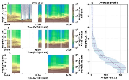
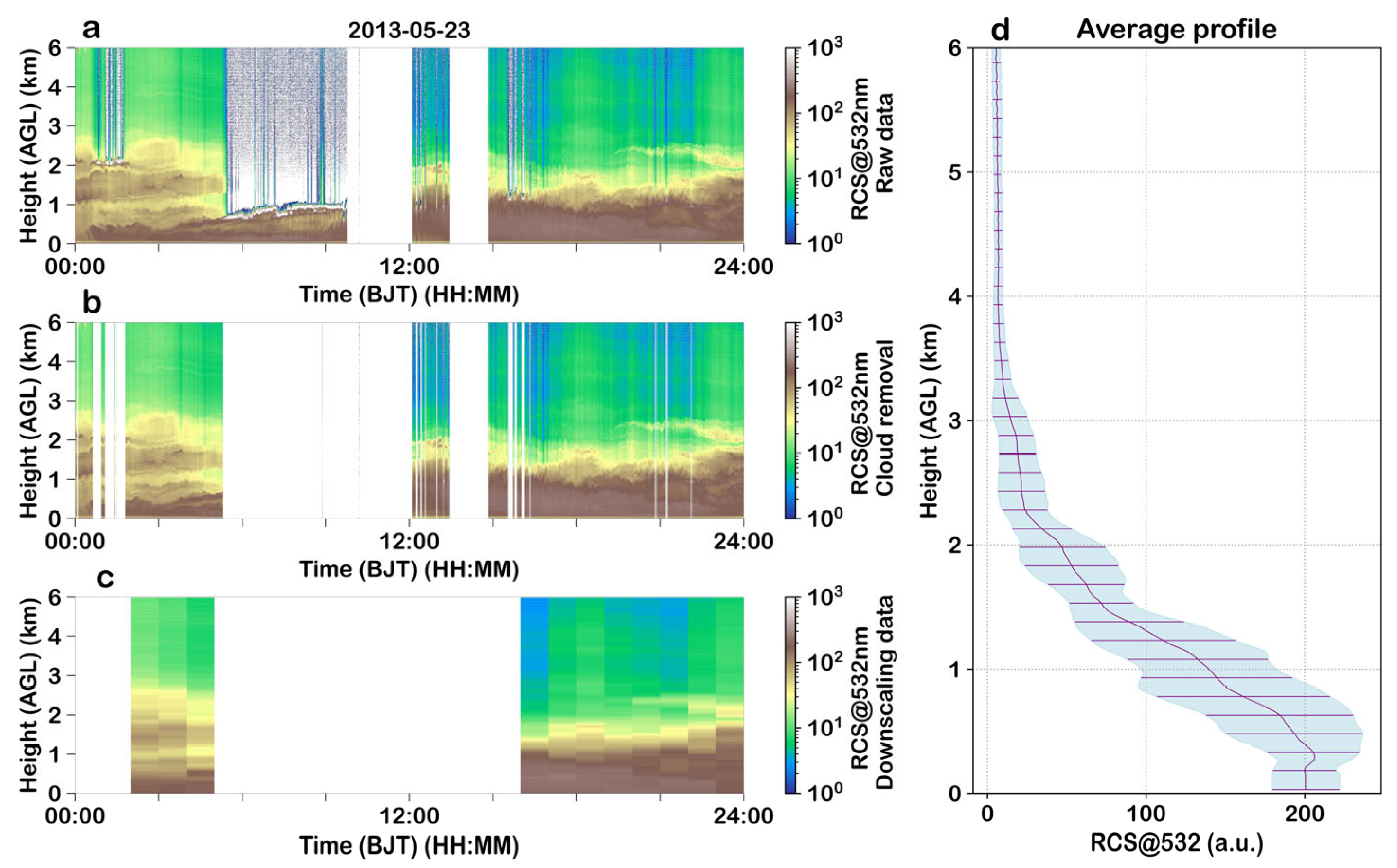
Figure 1a shows the time–height cross-section of the raw range-corrected signal at 532 nm. The data were obtained at Zhejiang Jinhua observation site on 23 May 2013. Time is Beijing local time. Altitude is local altitude. The original resolution of the data is 30 s and 7.5 m, which was converted to 1 h and 30 m after dimensionality reduction processing. The color bar represents the intensity of the range-corrected Mie-scattering signal at the 532 nm wavelength of the lidar in logarithmic scale. The signal intensity is displayed on a logarithmic scale, illustrating the backscatter contributions from aerosols and clouds. After cloud-screening, Figure 1b presents the same cross-section with cloud contamination effectively removed, making the aerosol layering more clearly identifiable. Figure 1c displays the cross-section after temporal averaging and vertical down-sampling, where the reduced resolution enhances the signal-to-noise ratio while retaining key structural features. Figure 1d shows the corresponding daily mean vertical profile. The profile decreases with height, with strong near-surface returns (0–1 km) reflecting high aerosol concentrations, followed by rapid attenuation above 2 km, where the narrower standard deviation range indicates relatively uniform and low aerosol loading aloft.
Figure 1.
Preprocessing and diurnal average variation of lidar atmospheric backscatter signals. (a) Time–height cross-section of raw lidar echo signals. (b) Time–height cross-section of lidar echo signals after cloud-screening processing. (c) Time–height cross-section of lidar echo signals after dimensionality reduction processing. (d) Average vertical profile of lidar echo signals, where the purple solid line represents the average profile and the light blue shadow denotes the standard deviation range of the data.
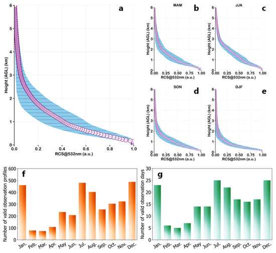
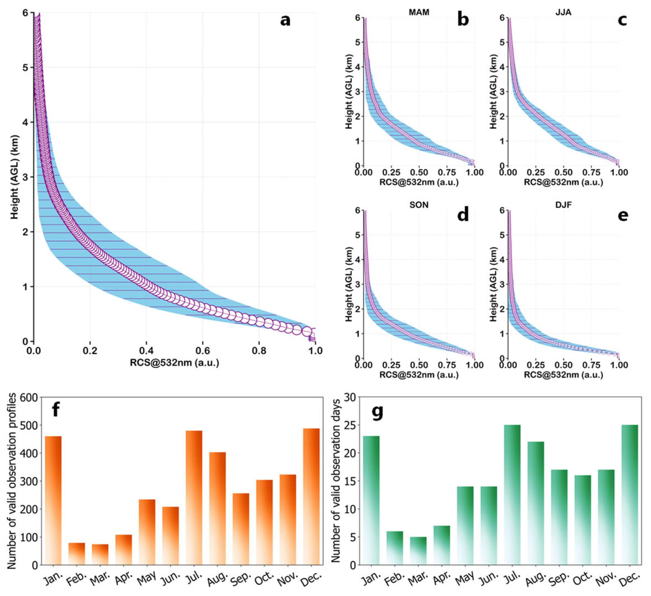
Figure 2a shows the annual mean vertical profile of the 532 nm lidar echo signal. The profile exhibits a typical decreasing pattern with height: strong returns near the surface indicate high aerosol loading, followed by rapid attenuation with increasing altitude. Above 2 km, the signal intensity becomes notably weaker. The standard deviation is largest between 1 and 2 km, suggesting stronger variability in aerosol layering within this height range. Seasonal mean profiles for spring (March-April-May, MAM), summer (June-July-August, JJA), autumn (September-October-November, SON), and winter (December-January-February, DJF) are shown in Figure 2b–e. The seasonal differences are distinct. Summer profiles attenuate more slowly with height, consistent with a higher boundary layer, stronger convection, and more efficient vertical mixing of aerosols. In contrast, winter profiles show faster attenuation and a narrower standard deviation range, reflecting lower boundary-layer heights and the tendency for aerosols to accumulate near the surface.
Figure 2.
Lidar observation sample conditions and seasonal variations of normalized average vertical profiles of 532 nm wavelength echo signals. (a) Annual average vertical profile of lidar echo signals, with blue shadows indicating the standard deviation range. (b–e) Average vertical profiles of lidar echo signals for spring (MAM), summer (JJA), autumn (SON), and winter (DJF), respectively, with blue shadows representing the standard deviation range. (e) Statistics of the number of valid observed profiles per month. (f) Statistics of the number of valid observed profiles per month. (g) Statistics of the number of valid observation days per month.
Figure 2f summarizes the number of valid lidar profiles obtained each month, illustrating the seasonal variability in data availability. Months such as January, July, and December exhibit a larger number of valid profiles, whereas February and early-spring months show fewer profiles due to more frequent precipitation and cloud cover. Figure 2g presents the number of valid observation days per month. January, July, and December record more continuous observations, while February to April have fewer valid days, again reflecting the influence of monthly weather conditions on lidar performance.
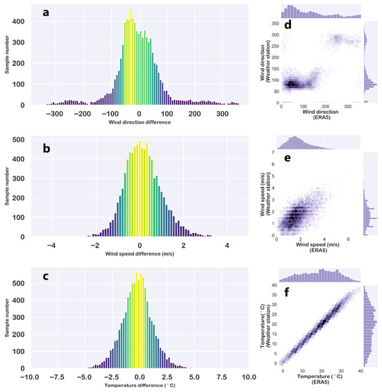
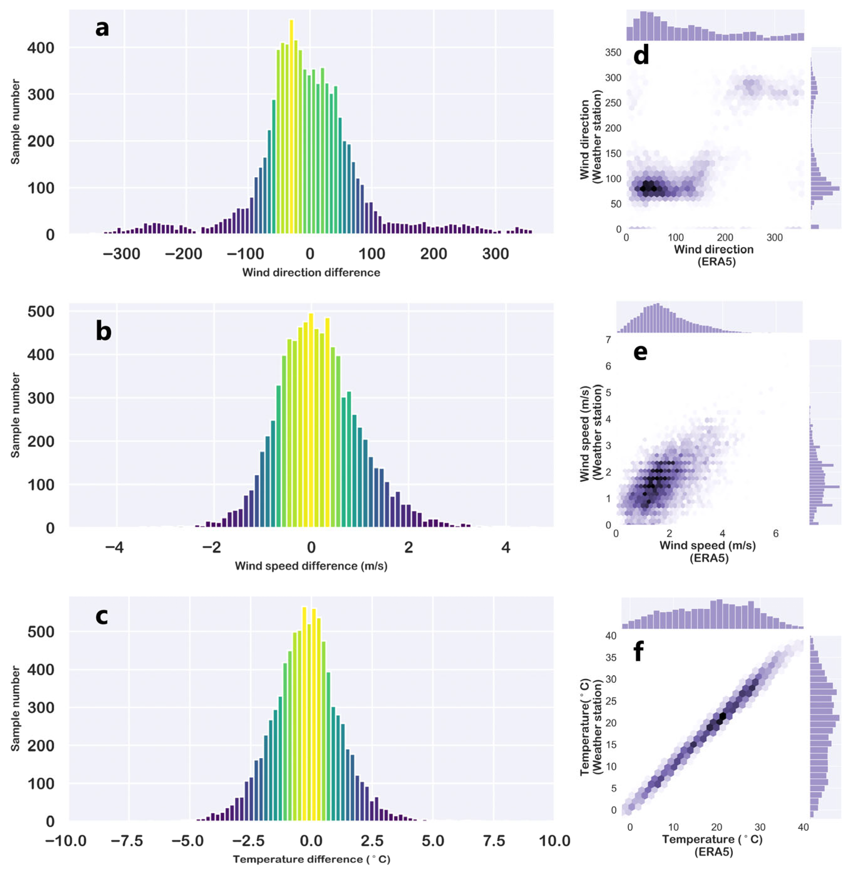
Figure 3 compares ground-based meteorological observations with ERA5 reanalysis data in terms of wind direction, wind speed, and temperature. The histogram of wind direction differences in Figure 3a shows a symmetric distribution centered around 0°, indicating that discrepancies between the two datasets generally fluctuate near zero and are mostly small, demonstrating good consistency in wind direction representation. Similarly, Figure 3b shows wind speed differences concentrated around 0 m/s, suggesting that ERA5 closely reproduces the observed wind speed. Temperature differences in Figure 3c also center around 0 °C, with most values falling within a narrow range, reflecting strong agreement between observed and reanalysis temperature fields.
Figure 3.
Correlation of meteorological elements between meteorological station and ERA5 reanalysis data. (a–c) Histograms of sample number distribution for differences in wind direction, wind speed, and temperature between meteorological station and ERA5 reanalysis data, with the ordinate representing the number of samples. (d–f) Scatter distributions and marginal distributions of wind direction, wind speed, and temperature between meteorological station and ERA5 reanalysis data. Wind direction data are derived from the synthesis of ERA5 u and v wind components.
The corresponding scatterplots in Figure 3d–f, along with their marginal distributions, further illustrate the degree of correspondence. Wind direction points in Figure 3d align broadly along the diagonal, although with slightly larger dispersion compared to the other variables. Wind speed in Figure 3e shows a tighter clustering along the diagonal, indicating stronger agreement. Temperature in Figure 3f exhibits a clear linear relationship with points closely following the diagonal, confirming the high fidelity of ERA5 temperature relative to ground observations. Overall, ERA5 reanalysis data demonstrate strong consistency with surface meteorological station measurements in wind and temperature, supporting their combined use in subsequent analyses.
3.2. Analysis of Aerosol Layer Structure and Meteorological Factors
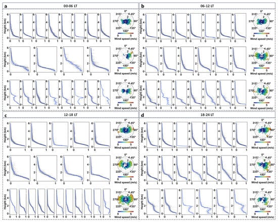
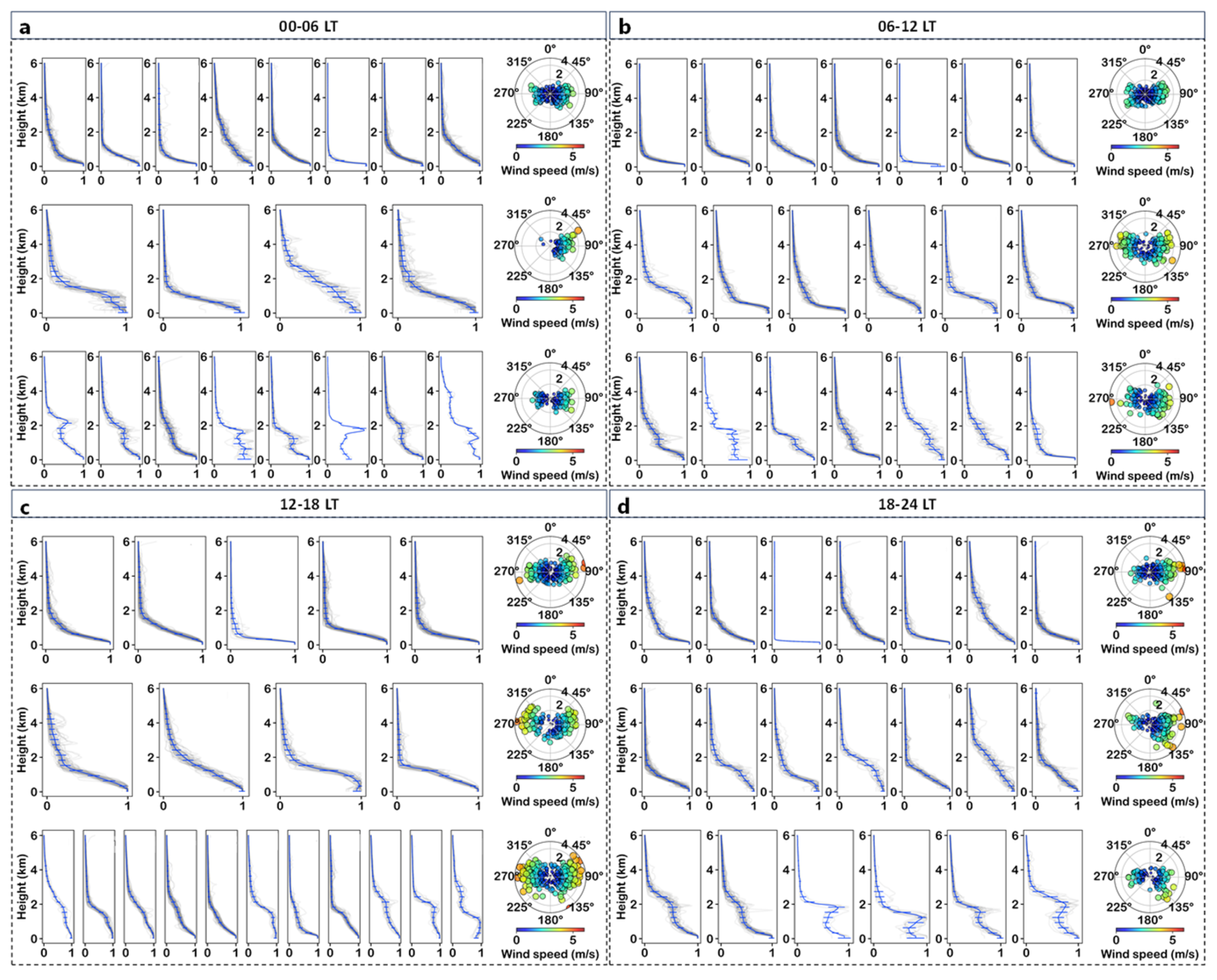
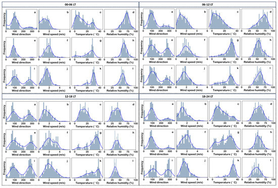
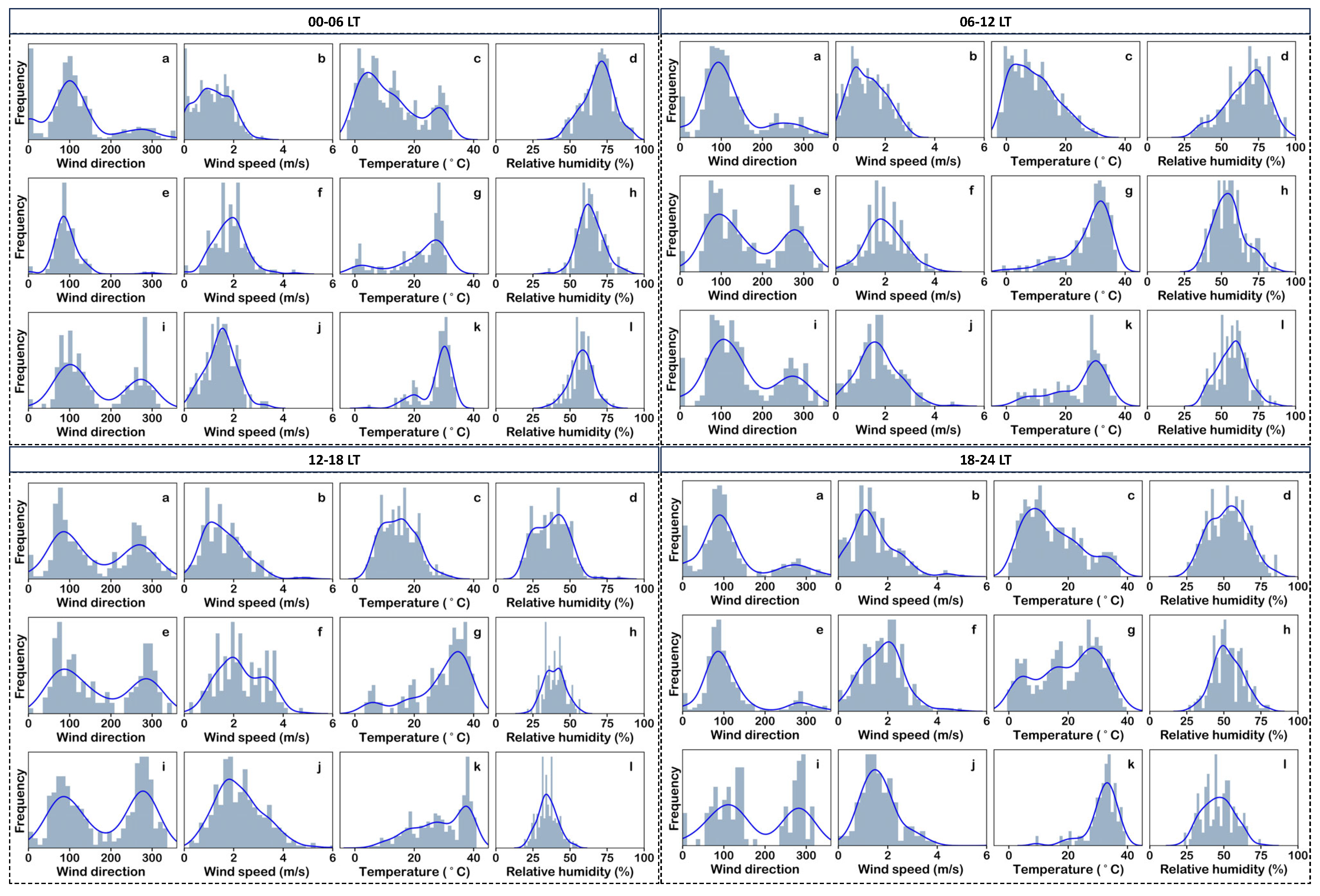
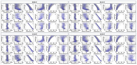
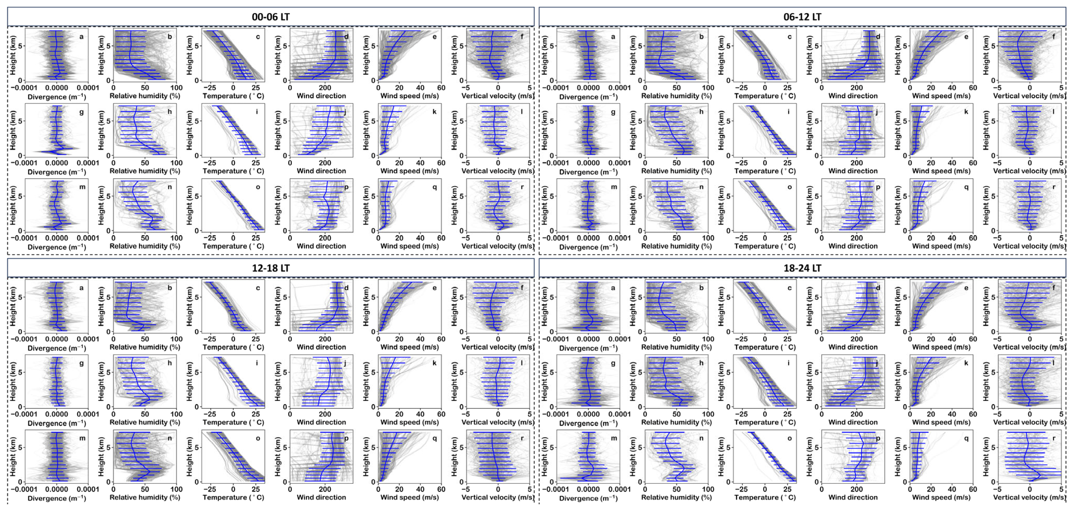
Figure 4, Figure 5 and Figure 6 summarize the relationships between aerosol vertical profile types and corresponding surface and ERA5 meteorological conditions. During the 00–06 LT period, for the single-layer convex aerosol structure, the surface wind field is dominated by easterlies. For the single-layer concave and multi-layer aerosol structures, the surface wind direction exhibits a bimodal distribution, with westerlies appearing in addition to easterlies. Another notable difference lies in the surface temperature: all three aerosol structures show a bimodal temperature distribution. The single-layer convex structure is mainly characterized by a primary peak at 25 °C and a secondary peak at around 0 °C. The single-layer concave structure is dominated by low temperatures. The multi-layer structure is primarily marked by a peak at 25 °C and a secondary peak at 20 °C. The surface wind speed distribution of the single-layer concave structure has a peak at 1 m/s, while the peaks of the other two structures are close to 2 m/s. Based on the vertical distribution of ERA5 meteorological factors, the upper-level wind speed of the single-layer concave structure differs from that of the other two. In contrast, the relative humidity, temperature, and wind direction of the multi-layer structure are distinct from those of the other two.
Figure 4.
Clustering analysis of atmospheric normalized backscatter profiles and ground wind field distribution (a–d). The clustering analysis selects 20 types (represented by curves). Gray represents the vertical distribution of this type of profile, and the blue line represents the distribution of the average profile. According to the distribution of the average profile, the 20 types are further divided into three structures: single-layer concave structure, single-layer convex structure, and multi-layer structure, which are presented in the first, second, and third columns of the figure respectively. The rightmost column of each row corresponds to the distribution characteristics of wind direction and wind speed (represented by scatter plots).
Figure 5.
Frequency distribution of surface meteorological elements. Each row represents the vertical profile of a different structure (a–l), corresponding to Figure 4. The gray bars are frequency statistics, and the blue curves are kernel density estimates.
Figure 6.
Vertical distribution of ERA5 meteorological profiles. Each row represents the vertical profile of a different structure (a–r), corresponding to Figure 4. The gray profiles indicate meteorological factors, and the blue curves are average profiles.
During the 06–12 LT period, surface meteorological factors indicate that the wind direction distribution is bimodal, while other factors mainly show a unimodal distribution. The multi-layer and single-layer convex structures exhibit relatively similar surface meteorological factor distribution characteristics. Meanwhile, the vertical distribution of ERA5 meteorological factors is also highly comparable, with the difference that the divergence of the multi-layer structure shows negative values (convergence) near the surface. The meteorological configuration of the single-layer concave structure during 06–12 LT is relatively consistent with that during 00–06 LT. Similarly, the meteorological configuration of the multi-layer structure in this period is also consistent with that in the 00–06 LT period.
During the 12–18 LT period, surface meteorological factors show that the meteorological configurations corresponding to the three aerosol types are relatively consistent, except for the surface temperature distribution. The surface temperature of the single-layer concave structure presents a unimodal distribution, while the other two types exhibit a bimodal distribution. In terms of ERA5 meteorological factors, the distributions of the three types are relatively consistent, except that the single-layer concave structure has higher upper-level wind speeds.
During the 18–24 LT period, compared with other time periods, the near-surface convergence and divergence motions are enhanced, and the vertical velocity changes are also more significant. Variations in wind speed, relative humidity, wind direction, and temperature all contribute to the formation of the multi-layer aerosol structure.
3.3. Boruta-Based Meteorological Attribution Analysis
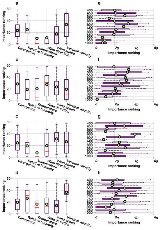
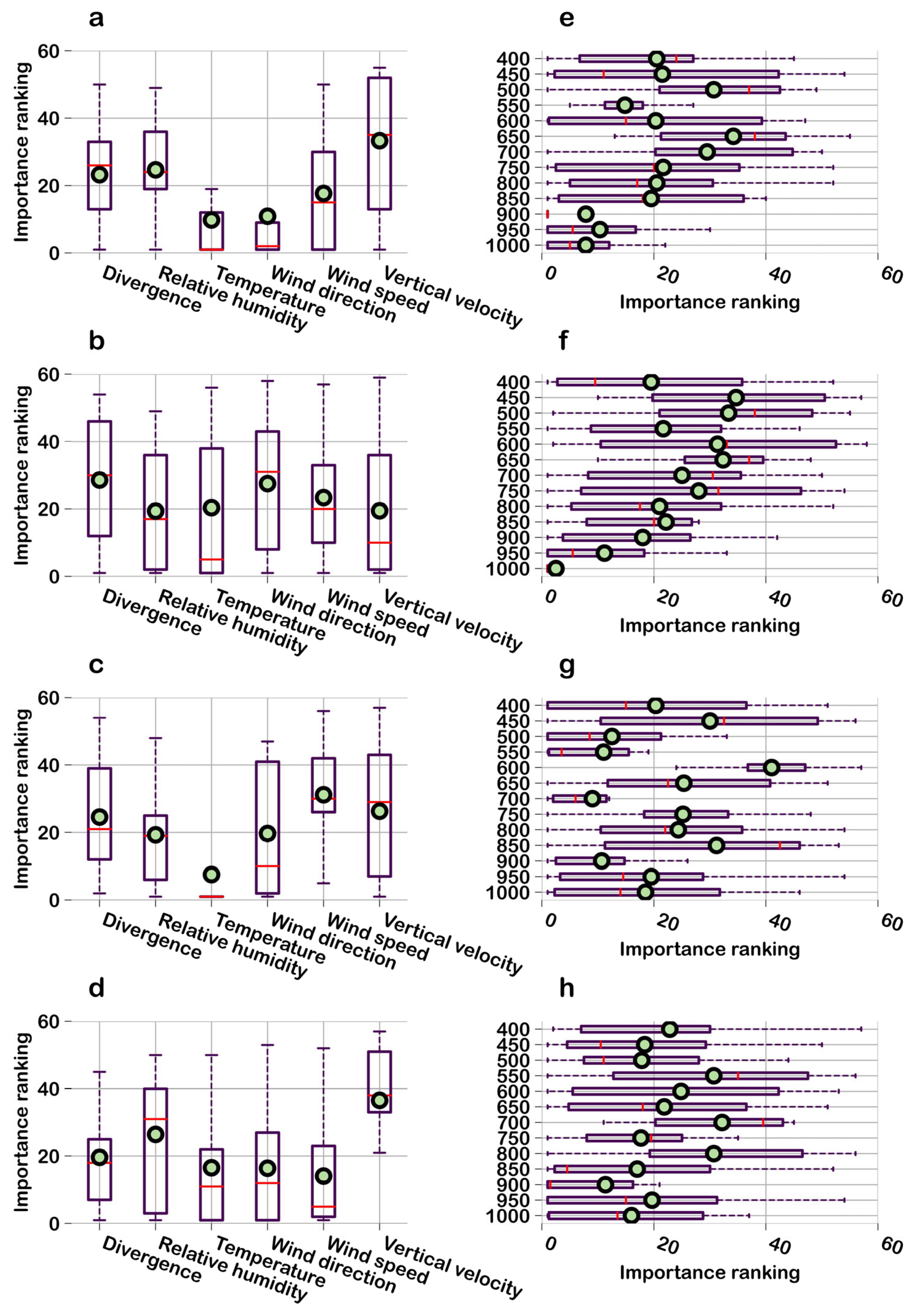
Combining the box plots in Figure 7a–d, the importance of six ERA5 meteorological factors, divergence, relative humidity, temperature, wind direction, wind speed, and vertical velocity, during the periods of 0–6, 6–12, 12–18, and 18–24, was analyzed using the Boruta algorithm. A smaller importance ranking value indicates a more important feature, and a smaller mean value (represented by the dots in the box plot) signifies a more prominent importance of the factor. The dispersion degree of the importance ranking of meteorological factors varies significantly with time periods. In terms of the mean value, this dispersion degree is the smallest during the 6–12 LT period. During this period, relative humidity, vertical velocity, and temperature exhibit the smallest importance ranking values, indicating that these three factors are the primary regulators of aerosol layer structure changes. Between the 0–6 LT and 12–18 LT periods, the key distinction is that wind speed ranks among the top three in the 0–6 LT period, while relative humidity enters the top three in the 12–18 LT period. The distribution patterns of the importance rankings are relatively similar between the 0–6 LT and 18–24 LT periods. Temperature, wind direction, and wind speed all feature in the top three of the importance ranking in both periods; however, wind speed becomes the dominant factor during the 18–24 LT period. Among all meteorological factors, divergence never enters the top three of the importance ranking.
Figure 7.
Boxplot distribution of Boruta importance rankings for the ERA5 six meteorological elements during the periods of 0–6, 6–12, 12–18, and 18–24 ((a–d) represent the importance of meteorological factors, and (e–h) represent the importance of height). The dots represent the mean value of the importance ranking for each element (the smaller the mean value, the more important the element), and the boxplots reflect the central tendency and dispersion of the importance rankings. The left side illustrates the variation of importance with meteorological factors, while the right side illustrates the variation of importance with height (the ordinate represents air pressure in hPa).
Figure 7e–h on the right illustrates the variation characteristics of importance with height (or relevant vertical levels). During the 0–6 LT and 6–12 LT periods, the importance rankings at different heights show a decreasing trend with increasing altitude. This trend is most pronounced in the 6–12 LT period compared to the 0–6 LT period. In the 12–18 LT period, the importance rankings exhibit a relatively disordered state. During the 18–24 LT period, the importance rankings also show a decreasing trend with increasing altitude, but this trend is weaker than that in the 0–6 LT and 6–12 LT periods, as the difference in the mean importance ranking between the lower and upper layers is smaller during the 18–24 LT period.
3.4. Meteorological–Aerosol Interaction Mechanisms
In summary, the single-layer concave aerosol structure is typically associated with lower surface temperature, higher surface relative humidity, and stronger upper-level wind speed. The single-layer convex aerosol structure matches moderate surface temperature, moderate surface relative humidity, and reduced upper-level wind speed. In contrast, the multi-layer aerosol structure is characterized by the highest surface temperature, a stratification of relative humidity at approximately 2 km altitude, and the weakest upper-level wind speed in terms of meteorological factor configuration.
The corresponding meteorological–aerosol mechanisms can be interpreted as follows. Under low surface temperature and high humidity, a surface-based temperature inversion forms, suppressing near-surface buoyancy generation, weakening turbulent kinetic energy, and limiting vertical eddy diffusion of aerosol particles. The enhanced upper-level wind speed induces shear, but this shear remains decoupled from the stagnant near-surface layer, resulting in the accumulation of aerosols within a single, concave-shaped layer.
When the surface undergoes moderate heating, the inversion weakens and shallow convective motions develop. Near-surface convergence and divergence cells begin to emerge, enabling intermittent vertical lifting of aerosols. Reduced upper-level wind speed decreases shear-driven ventilation, causing the vertical profile to become more uniform and convex. Under these conditions, local entrainment at the top of the shallow mixing layer can intermittently transport aerosol plumes upward, but the lack of strong humidity stratification prevents formation of distinct elevated sublayers.
As surface temperature increases further, enhanced buoyancy breaks the residual inversion and deepens the convective boundary layer. At the same time, the prominent stratification of relative humidity at around 2 km altitude promotes aerosol hygroscopic growth and favors formation of elevated aerosol layers through phase transitions and water uptake. Meanwhile, the markedly weakened upper-level wind reduces long-range advection and shear dispersion, which allows lofted aerosols to remain suspended and separate into multiple distinct layers. Vertical velocity perturbations and weak divergence near the surface further facilitate repeated lifting and settling cycles, ultimately yielding a stable multi-layer aerosol structure with humid, lofted layers superimposed above a heated surface layer.
4. Discussion and Conclusions
This study investigates the dynamic characteristics of aerosol vertical distribution within the atmospheric boundary layer by integrating multi-source observational data, including ground meteorological measurements, ERA5 reanalysis, and lidar-derived aerosol vertical profiles. By constructing an analytical framework linking “meteorological factors to aerosol vertical structure,” we exhibited distributions of aerosol profile types and corresponding meteorological variables across different time periods. The Boruta algorithm was then applied to quantitatively assess the relative importance of six key meteorological variables, divergence, relative humidity, temperature, wind direction, wind speed, and vertical velocity, during four characteristic time windows (00–06, 06–12, 12–18, and 18–24 LT).
Through the identification of representative aerosol vertical structures (single-layer concave, single-layer convex, and multi-layer types) and their associated surface and upper-air meteorological conditions, an initial qualitative linkage between aerosol layering and meteorological states was established. The quantitative results from Boruta further reveal pronounced temporal contrasts in the influence of each meteorological factor, reflecting the diurnal evolution of boundary-layer stability, turbulence intensity, and thermodynamic structure. These variations highlight the inherently non–steady-state nature of meteorological controls on aerosol vertical distribution.
However, several limitations remain. First, the analysis focuses on four time periods within a single diurnal cycle and does not incorporate long-term seasonal or interannual variability. Second, the spatial representation is limited to one observational site and may not fully capture regional-scale aerosol–meteorology interactions. Third, the atmospheric environment involves complex nonlinear coupling among meteorological variables and between meteorology and aerosols, and such interactions are only partially captured in the present framework. Fourth, the range-corrected signal incorporates the Rayleigh scattering contribution of atmospheric molecules, which is affected by temperature and thus introduces errors into the analysis of aerosol layer structure. Finally, preprocessing involving cloud-screening and down-sampling affects the number of valid profiles, and it is also found that the number of valid profiles is relatively small in spring, thereby introducing additional errors.
Future work should extend observational and analytical efforts to broader temporal and spatial scales and investigate the nonlinear, multi-factor coupling mechanisms that modulate aerosol vertical structure. Aerosol types will also be incorporated into the analysis. Such efforts would allow for a more comprehensive and accurate understanding of the processes governing aerosol vertical evolution.
Author Contributions
S.Y. contributed to conceptualization, methodology, writing—original draft and writing—reviewing; W.X. contributed to investigation and data curation; D.L. contributed to supervision and resources; P.L. contributed to investigation and validation; T.G. contributed to supervision. All authors have read and agreed to the published version of the manuscript.
Funding
The work is supported by the Dreams Foundation of Jianghuai Advanced Technology Center (No. 2023-ZM01K008).
Data Availability Statement
The data that support the findings of this study are available from the corresponding author upon reasonable request.
Conflicts of Interest
Author Wanyi Xie was employed by the company Jianghuai Advanced Technology Center. The remaining authors declare that the research was conducted in the absence of any commercial or financial relationships that could be construed as a potential conflict of interest.
References
- Khain, A.; Pinsky, M.; Korolev, A. Combined effect of the wegener-bergeron-findeisen mechanism and large eddies on microphysics of mixed-phase stratiform clouds. J. Atmos. Sci. 2022, 79, 383–407. [Google Scholar] [CrossRef] [Scilit]
- Yin, J.; Mao, Z.; Jiang, P.; De Lombaerde, E.; Ye, J.; Fang, S.; Lin, F.; Lu, X.; Wang, X. Seasonal variations in the mechanisms of understory herb diversity in a temperate forest in Northeast China. Ecol. Indic. 2024, 160, 111827. [Google Scholar] [CrossRef] [Scilit]
- Cao, Z.; Zhu, D.; Zhao, Y.; Xiao, H.; Li, R.; Fu, L. Coupling and coordination of rainfall erosivity and aerosols in the pearl river basin under multiple shared socio-economic pathways. Theor. Appl. Climatol. 2024, 155, 6053–6067. [Google Scholar] [CrossRef] [Scilit]
- Li, Y.; Shang, Y.; Zheng, C.; Ma, Z. Estimated acute effects of ozone on mortality in a rural district of Beijing, China, 2005–2013: A time-stratified case-crossover study. Int. J. Environ. Res. Public Health 2018, 15, 2460. [Google Scholar] [CrossRef] [Scilit] [PubMed]
- Joharestani, M.Z.; Cao, C.; Ni, X.; Bashir, B.; Talebiesfandarani, S. PM2.5 prediction based on random forest, xgboost, and deep learning using multisource remote sensing data. Atmosphere 2019, 10, 373. [Google Scholar] [CrossRef] [Scilit]
- He, C.; Kumar, R.; Tang, W.; Pfister, G.; Xu, Y.; Qian, Y.; Brasseur, G. Air pollution interactions with weather and climate extremes: Current knowledge, gaps, and future directions. Curr. Pollut. Rep. 2024, 10, 430–442. [Google Scholar] [CrossRef] [Scilit]
- Li, Y.; Zhang, M.; Ma, G.; Ren, H.; Yu, E. Analysis of primary air pollutants’ spatiotemporal distributions based on satellite imagery and machine-learning techniques. Atmosphere 2024, 15, 287. [Google Scholar] [CrossRef] [Scilit]
- Di, H.; Li, S.; Yuan, Y.; Hua, D.; Wang, J. Observational study of the vertical aerosol and meteorological factor distributions with respect to particulate pollution in Xi’an. Atmos. Environ. 2021, 247, 118215. [Google Scholar] [CrossRef] [Scilit]
- Gidarakou, M.; Papayannis, A.; Kokkalis, P.; Evangeliou, N.; Vratolis, S.; Remoundaki, E.; Zwaaftink, C.G.; Eckhardt, S.; Veselovskii, I.; Mylonaki, M.; et al. Optical and microphysical properties of the aerosols during a rare event of biomass-burning mixed with polluted dust. Atmosphere 2024, 15, 190. [Google Scholar] [CrossRef] [Scilit]
- Griesche, H.J.; Seifert, P.; Engelmann, R.; Radenz, M.; Hofer, J.; Althausen, D.; Walbröl, A.; Barrientos-Velasco, C.; Baars, H.; Dahlke, S.; et al. Cloud micro- and macro-physical properties from ground-based remote sensing during the mosaic drift experiment. Sci. Data 2024, 11, 505. [Google Scholar] [CrossRef] [Scilit]
- Eswaran, K.; Montoux, N.; Chauvigné, A.; Baray, J.-L.; Ancellet, G.; Sellegri, K.; Freney, E.; Rose, C.; Pelon, J. Lidar ratio calculations from in situ aerosol optical, microphysical and chemical measurements: Observations at puy de dome, France and analysis with caliop. Atmos. Res. 2023, 296, 107043. [Google Scholar] [CrossRef] [Scilit]
- Zhang, T.; Zhang, R.; Zhong, J.; Che, H.; Wang, J.; Guo, L. The vertical pollution structure reflected by aerosol optical properties in Beijing and its relation with meteorological conditions in the autumn and winter of 2017–2020. Atmos. Environ. 2023, 308, 119870. [Google Scholar] [CrossRef] [Scilit]
- Sun, W.; Liu, Z.; Zhang, Y.; Zhang, J.; Lv, Z. Contrast observation of aerosol vertical structure by space-borne lidar and ground-based lidar in Yibin area. Environ. Monit. China 2019, 35, 150–160. [Google Scholar]
- Nie, X.; Mao, Q. Study on inversion of atmospheric aerosol nonsphericity based on satellite and ground observations. Atmos. Res. 2023, 283, 106582. [Google Scholar] [CrossRef] [Scilit]
- Wang, L.; Stanic, S.; Eichinger, W.; Mocnik, G.; Drinovec, L.; Gregoric, A. Investigation of aerosol properties and structures in two representative meteorological situations over the vipava valley using polarization Raman lidar. Atmosphere 2019, 10, 128. [Google Scholar] [CrossRef] [Scilit]
- Engelmann, R.; Wandinger, U.; Ansmann, A.; Mueller, D.; Zeromskis, E.; Althausen, D.; Wehner, B. Lidar Observations of the vertical aerosol flux in the planetary boundary layer. J. Atmos. Ocean. Technol. 2008, 25, 1296–1306. [Google Scholar] [CrossRef] [Scilit]
- Schmidt, J.; Ansmann, A.; Buehl, J.; Baars, H.; Wandinger, U.; Mueller, D.; Malinka, A.V. Dual-fov raman and doppler lidar studies of aerosol-cloud interactions: Simultaneous profiling of aerosols, warm-cloud properties, and vertical wind. J. Geophys. Res. Atmos. 2014, 119, 5512–5527. [Google Scholar] [CrossRef] [Scilit]
- Zhang, T.; Che, H.; Gong, Z.; Wang, Y.; Wang, J.; Yang, Y.; Gui, K.; Guo, B. The two-way feedback effect between aerosol pollution and planetary boundary layer structure on the explosive rise of PM2.5 after the “ten statements of atmosphere” in Beijing. Sci. Total Environ. 2020, 709, 136259. [Google Scholar] [CrossRef] [Scilit]
- Pal, S.; Haeffelin, M.; Batchvarova, E. Exploring a geophysical process-based attribution technique for the determination of the atmospheric boundary layer depth using aerosol lidar and near-surface meteorological measurements. J. Geophys. Res. Atmos. 2013, 118, 9277–9295. [Google Scholar] [CrossRef] [Scilit]
- Wang, C.; Jia, M.; Xia, H.; Wu, Y.; Wei, T.; Shang, X.; Yang, C.; Xue, X.; Dou, X. Relationship analysis of PM2.5 and boundary layer height using an aerosol and turbulence detection lidar. Atmos. Meas. Tech. 2019, 12, 3303–3315. [Google Scholar] [CrossRef] [Scilit]
- Devara, P.C.S.; Raj, P.E.; Sharma, S.; Pandithurai, G. Lidar-observed long-term variations in urban aerosol characteristics and their connection with meteorological parameters. Int. J. Climatol. 1994, 14, 581–591. [Google Scholar] [CrossRef] [Scilit]
- Myasnikov, A.V.; Pershin, S.M.; Grishin, M.Y.; Zavozin, V.A.; Makarov, V.S.; Ushakov, A. Estimation of the influence of meteorological factors on the aerosol lidar signal in tunnels above the elbrus volcano chamber. Phys. Wave Phenom. 2022, 30, 119–127. [Google Scholar] [CrossRef] [Scilit]
- Li, X.; Tian, Y.; Yang, M.; Wang, S. Cumulative effects of meteorological factors on low-flow change in the upper yellow river. Theor. Appl. Climatol. 2024, 155, 8717–8730. [Google Scholar] [CrossRef] [Scilit]
- Liu, Y.; Gui, K.; Chen, Q.; Feng, L.; Cai, H.; Zhang, X.; Yao, W.; Zhao, H.; Shang, N.; Li, L.; et al. Three-dimensional structure and transport flux of springtime smoke aerosols over the indochina peninsula. Atmos. Res. 2024, 301, 107293. [Google Scholar] [CrossRef] [Scilit]
- Dong, L.; Wang, M.; Rosenfeld, D.; Zhu, Y.; Wang, Y.; Dong, X.; Liu, Z.; Wang, H.; Zeng, Y.; Cao, Y.; et al. Effects of smoke on marine low clouds and radiation during 2020 western united states wildfires. Atmos. Res. 2024, 302, 107295. [Google Scholar] [CrossRef] [Scilit]
- Noh, Y.M.; Shin, D.H.; Müller, D. Variation of the vertical distribution of nabro volcano aerosol layers in the stratosphere observed by lidar. Atmos. Environ. 2017, 154, 1–8. [Google Scholar] [CrossRef] [Scilit]
- Zhou, T.; Xie, H.; Bi, J.; Huang, Z.; Huang, J.; Shi, J.; Zhang, B.; Zhang, W. Lidar measurements of dust aerosols during three field campaigns in 2010, 2011 and 2012 over Northwestern China. Atmosphere 2018, 9, 173. [Google Scholar] [CrossRef] [Scilit]
- Xiong, Z.; Xu, X.; Yang, Y.; Luo, T. Diurnal vertical distribution and transport of dust aerosol over and around tibetan plateau from lidar on international space station. Atmos. Res. 2023, 294, 106939. [Google Scholar] [CrossRef] [Scilit]
- Li, Z.; Shi, H.; Yang, X.; Tang, H. Investigating the nonlinear relationship between surface solar radiation and its influencing factors in North China plain using interpretable machine learning. Atmos. Res. 2022, 280, 106406. [Google Scholar] [CrossRef] [Scilit]
- Nasonov, S.; Balin, Y.; Klemasheva, M.; Kokhanenko, G.; Novoselov, M.; Penner, I. Peculiarities of the vertical structure of atmospheric aerosol fields in the basin of lake baikal according to lidar observations. Atmosphere 2023, 14, 837. [Google Scholar] [CrossRef] [Scilit]
- Chiang, C.-W.; Das, S.K.; Lin, C.-Y.; Nee, J.B.; Sun, S.-H.; Chiang, H.-W.; Yu, M.-J.; Zhang, S.-T. Multi-year investigations of aerosol layer using lidar measurements at Chung-Li, Taiwan. J. Atmos. Sol.-Terr. Phys. 2012, 89, 40–47. [Google Scholar] [CrossRef] [Scilit]
- Gong, W.; Liu, B.; Ma, Y.; Zhang, M. Mie lidar observations of tropospheric aerosol over Wuhan. Atmosphere 2015, 6, 1129–1140. [Google Scholar] [CrossRef] [Scilit]
- Brakhasi, F.; Hajeb, M.; Mielonen, T.; Matkan, A.; Verbesselt, J. Investigating aerosol vertical distribution using calipso time series over the middle east and North Africa (mena), Europe, and India: A bfast-based gradual and abrupt change detection. Remote Sens. Environ. 2021, 264, 112619. [Google Scholar] [CrossRef] [Scilit]
- Assiri, M.E. Aerosol Types Identification over the Arabian Peninsula Using AERONET Products: Evaluation with Multisource Datasets. Earth Syst. Environ. 2024, 8, 483–499. [Google Scholar] [CrossRef] [Scilit]
- Song, T.; Wang, J.; Yu, X.; de Leeuw, G. Application of Gaussian Mixture Models for aerosol type analysis in China. Atmos. Res. 2023, 294, 106938. [Google Scholar] [CrossRef] [Scilit]
- Krishnaveni, A.S.; Madhavan, B.L.; Ratnam, M.V. Aerosol classification using fuzzy clustering over a tropical rural site. Atmos. Res. 2023, 282, 106518. [Google Scholar] [CrossRef] [Scilit]
- Jorquera, H.; Villalobos, A.M. Combining Cluster Analysis of Air Pollution and Meteorological Data with Receptor Model Results for Ambient PM2.5 and PM10. Int. J. Environ. Res. Public Health 2020, 17, 8455. [Google Scholar] [CrossRef] [Scilit]
- Li, Z.; D’Ambro, E.L.; Schobesberger, S.; Gaston, C.J.; Lopez-Hilfiker, F.D.; Liu, J.; Shilling, J.E.; Thornton, J.A.; Cappa, C.D. A robust clustering algorithm for analysis of composition-dependent organic aerosol thermal desorption measurements. Atmos. Chem. Phys. 2020, 20, 2489–2512. [Google Scholar] [CrossRef] [Scilit]
- Hameed, M.; Yang, F.; Bazai, S.U.; Ghafoor, M.I.; Alshehri, A.; Khan, I.; Ullah, S.; Baryalai, M.; Jaskani, F.H.; Andualem, M. Convolutional Autoencoder-Based Deep Learning Approach for Aerosol Emission Detection Using LiDAR Dataset. J. Sens. 2022, 2022, 3690312. [Google Scholar] [CrossRef] [Scilit]
- Boldeanu, M.; Cucu, H.; Burileanu, C.; Mărmureanu, L. Multi-Input Convolutional Neural Networks for Automatic Pollen Classification. Appl. Sci. 2021, 11, 11707. [Google Scholar] [CrossRef] [Scilit]
- Wang, J.; Liu, Y.; Chen, L.; Liu, Y.; Mi, K.; Gao, S.; Mao, J.; Zhang, H.; Sun, Y.; Ma, Z. Validation and calibration of aerosol optical depth and classification of aerosol types based on multi-source data over China. Sci. Total Environ. 2023, 903, 166603. [Google Scholar] [CrossRef] [Scilit]
- Yu, S.; Liu, D.; Xu, J.; Wang, Z.; Wang, Y. Optical properties and seasonal distribution of aerosol layers observed by lidar over Jinhua, Southeast China. Atmos. Environ. 2021, 257, 118456. [Google Scholar] [CrossRef] [Scilit]
Disclaimer/Publisher’s Note: The statements, opinions and data contained in all publications are solely those of the individual author(s) and contributor(s) and not of MDPI and/or the editor(s). MDPI and/or the editor(s) disclaim responsibility for any injury to people or property resulting from any ideas, methods, instructions or products referred to in the content. |
© 2026 by the authors. Licensee MDPI, Basel, Switzerland. This article is an open access article distributed under the terms and conditions of the Creative Commons Attribution (CC BY) license.