State of the Art in Monitoring Methane Emissions from Arctic–boreal Wetlands and Lakes

Highlights

What are the main findings?

• Arctic–boreal wetlands and lakes are major but highly uncertain methane sources
• Small lakes and winter emissions are poorly captured in current inventories.

What is the implication of the main finding?

• Combining top-down and bottom-up methods reduces methane estimate uncertainty.
• New satellites and explainable AI can strengthen high-latitude methane budgets.

Abstract

Arctic–boreal wetlands and lakes are among the most significant and most uncertain natural sources of atmospheric methane. Rapid Arctic amplification, permafrost thaw, hydrological change, and increasing ecosystem productivity are expected to intensify methane emissions from high-latitude landscapes. Yet, significant uncertainties persist in quantifying their magnitude, seasonality, and spatial distribution. This review synthesizes the current state of the art in monitoring methane emissions from Arctic–boreal wetlands and lakes through complementary bottom-up and top-down approaches. We examine Earth observation (EO) capabilities, including optical, thermal infrared (TIR), and synthetic aperture radar (SAR) missions, as well as new emerging satellite platforms. We also assess in situ measurement networks, wetland and lake inventories, empirical and process-based models, and atmospheric inversion frameworks. Key gaps remain in representing small waterbodies, shoreline heterogeneity, winter emissions, inventory harmonization, and integration between atmospheric retrievals and surface-based flux models. Moreover, advances in multi-sensor data fusion, explainable artificial intelligence (XAI), physics-informed inversion methods, and geospatial foundation models offer strong potential to reduce these uncertainties. A coordinated integration of satellite observations, field measurements, and transparent modeling frameworks is essential to improve Arctic–boreal methane budgets and strengthen projections of climate feedback in a rapidly warming region.

1. Introduction

Atmospheric methane is a potent driver of global warming, contributing nearly one-quarter of the observed warming to date [1]. Methane concentrations have more than tripled from approximately 600–700 parts per billion (ppb) in pre-industrial times to approximately 1930 ppb today [2], accelerating in the 1900s due to intensified agricultural activities and fossil fuel use [3]. Methane has a warming potential 84 times greater than carbon dioxide over a 20-year period. While anthropogenic sources are the dominant contributors to methane emissions related to human activities and the largest source of uncertainty [4], wetlands remain the largest natural source, representing an estimated 20% of global methane emissions [5,6]. Lakes and other inland waterbodies are also significant contributors to the natural methane budget, with aquatic ecosystems collectively accounting for approximately 11% of global natural methane emissions [7].

Wetlands are prominent features of the Arctic–boreal region, where they develop under waterlogged, oxygen-deprived conditions that facilitate the growth of methanogenic microorganisms [8]. Wetlands make up approximately 14% of the Arctic–boreal landscape and are underlain by permafrost (permanently frozen ground) [9,10,11,12]. Wetlands are projected to form the majority of the methane climate feedback by the year 2100 [13], with methane emissions from wetlands and lakes predicted to increase by an estimated 31%, largely as a result of climate warming [7]. The role of Arctic–boreal wetlands in methane emission is becoming more significant as warming in the Arctic is rising four times faster than the global average [14]. As organic-rich permafrost thaws, previously sequestered carbon is released into the atmosphere through increased microbial production of greenhouse gases such as methane and/or carbon dioxide, exacerbating warming and contributing to warming that accelerates the process [15].

Lakes and other waterbodies, while often grouped with wetlands, act as distinct methane sources with unique emission dynamics [16]. Temperature, ice freeze and thaw, water depth, microbial activity, and substrate availability regulate methane production, oxidation, and transport in lakes and other waterbodies [17]. In Arctic–boreal lakes, methane is primarily produced in sediments under anaerobic conditions and is released through ebullition, where gas bubbles containing methane rise to the surface and enter the atmosphere during open water conditions, while winter ice cover traps methane bubbles (e.g., Walter Anthony et al., [18]) with dissolved methane levels increasing until spring ice-out [16]. Although ebullition dominates methane release globally [19], diffusion plays a larger role under certain conditions [20]. Shallow lakes and windy periods cause strong turbulent mixing that carries dissolved methane upward at a fast rate [21]. This short residence time limits oxidation, allowing more methane to reach the surface. Thawing permafrost and warming climates facilitate the migration of methane from deep reservoirs through unfrozen zones (taliks) into lakes [22,23], mixing with biogenic and thermogenic sources [24]. Despite their importance, uncertainties remain in accurately quantifying methane fluxes from these lakes [25].

Wetland and lake extent remains a major source of uncertainty in bottom-up methane modeling [26]. Accurately extracting wetland extent is challenging due to the range of wetland expression [27,28,29], varying qualitative definitions [30], and short- and long-term inundation dynamics [31,32,33]. Some datasets may not distinguish between wetland classes, partly because remote sensing is challenging for extracting accurate wetland spatial information, given complex and shared spectral and spatial characteristics within and amongst different classes [34]. Lake emission estimates face similar challenges, including a lack of separation between wetlands and lakes in existing land cover classification datasets, dynamic uncertainties [35], and the small size of lakes [36,37].

Top-down methodologies rely on atmospheric methane measurements combined with inverse modeling to estimate methane budgets [38]. Satellite-mounted instruments used for this purpose span multiple spectral domains, such as the TROPOspheric Monitoring Instrument (TROPOMI), and various thermal infrared sensors, such as the Infrared Atmospheric Sounding Interferometer (IASI), which enhance these approaches by measuring methane concentrations across large regions, offering frequent observations, though Arctic–boreal applications face challenges. In contrast, bottom-up approaches integrate land cover datasets with methane flux inventories or process-based models to extrapolate emissions across regional scales [39] using techniques such as eddy covariance (EC) [40] and plot-scale chambers. Chambers are simple to deploy and provide local information important for understanding methane emission processes related to microtopography and vegetation [41,42]. They offer limited spatial coverage and frequency of sampling [43]. EC Flux towers provide site-scale ecosystem-scale methane flux data at high temporal resolution, but have a sparse distribution across Arctic–boreal regions due to the need for extensive resources [44]. New approaches applying artificial intelligence (AI) machine learning techniques, such as random forests and neural networks, are being developed to upscale sparse EC measurements and improve spatial coverage of carbon flux estimates (e.g., Skeeter et al., [45] and Jung et al., [46]). Satellite-based observations complement both top-down and bottom-up methods by providing critical biophysical and biogeochemical variables, such as frozen or thawed surface conditions (e.g., lake-ice or snow-cover dynamics, soil moisture and surface temperature, and extents of wetlands and lakes) [47,48,49,50], serving as proxies for methane flux estimation.

Bottom-up approaches frequently yield higher estimates than top-down [51], with disparities arising from diverse emission rates across different sources, atmospheric measurement uncertainties, and atmospheric transport and chemistry complexities [52]. These challenges are further compounded by double-counting, wherein the same emissions are counted multiple times across different models or datasets [17]. Another key issue involves the coarse spatial resolution of many existing satellite-based inventories, which can miss water bodies even though they are recognized as methane emission hotspots [53]. The absence of small features can introduce significant errors and uncertainties into bottom-up inventories, making it difficult to accurately represent the full extent of methane fluxes [37]. Achieving higher-resolution observations and more frequent measurements is therefore crucial for differentiating between emission sources and reducing both double-counting and omission errors in Arctic–boreal methane assessments.

Given recently launched and upcoming satellite missions and advances in AI, this paper aims to summarize what can be expected in future estimates of Arctic–boreal methane emissions. First, a summary of current and upcoming Earth observation (EO) data capable of extracting wetland and lake features relevant to methane monitoring, and of satellites capable of detecting and mapping surface characteristics tied to methane flux. This includes a discussion of the applications of EO data for mapping wetlands and lakes, as well as emerging EO technologies. Second, a summary of current methods for estimating methane in wetlands and lakes using bottom-up techniques, including in situ data collection methods, available wetland and lake inventories, and recent process-based and data-driven models. Third is a summary of top-down models. Finally, a discussion of current knowledge gaps that require further investigation to improve both global and regional estimates of wetland and lake emissions.

2. Earth Observation Data for Wetland and Lake Mapping and Methane Monitoring

EO applications for monitoring methane emissions from lakes and wetlands span two complementary purposes: (1) detection and quantification of atmospheric methane using infrared sensors [38] using optical and thermal satellite sensors, which support top-down emission estimation, and (2) spatial mapping of biophysical features that exert control on methane emission [54], which supports bottom-up approaches.

2.1. Multispectral Satellites

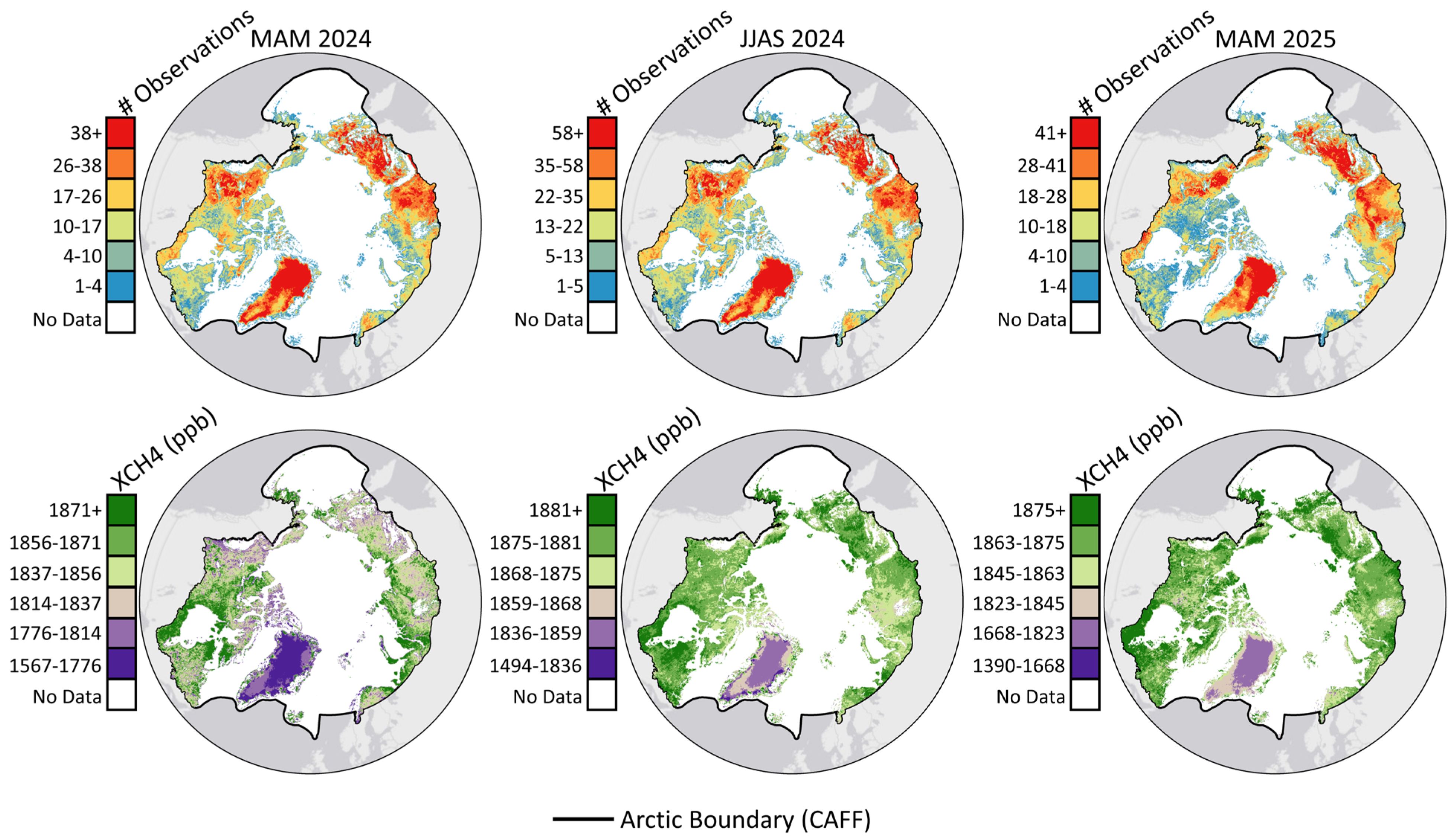
Optical instruments carried by satellites are among the most widely used sources of EO data due to their intuitive interpretation and the widespread, free accessibility of missions such as Sentinel-5P, Sentinel-2, Sentinel-1, and Landsat. Optical instruments used for atmospheric methane detection can be categorized into two types: area flux mappers, such as TROPOMI or GOSAT, and point source imagers, such as Greenhouse Gas Satellite (GHGSat) [55,56]. However, retrieval of data using optical sensors faces numerous challenges in the Arctic–boreal regions that significantly limit year-round monitoring capabilities, including persistent cloud cover and adverse weather conditions that block solar radiation, extended periods of darkness during the winter months, and generally shorter daylight hours, and snow and ice surfaces that impact albedo and retrieval accuracy. The impact of these limitations is illustrated in Figure 1, which presents a seasonal comparison of TROPOMI observations over Arctic–boreal regions, highlighting the availability of methane column measurements across seasons. During winter, many Arctic–boreal areas are entirely missed, receiving no high-quality observations for methane column estimation (i.e., the retrieval of the total amount of methane present in a vertical slice of atmosphere from the Earth’s surface to the top of the atmosphere expressed as a column-averaged dry-air mole fraction). This seasonal limitation indicates a key obstacle for year-round, top-down methane monitoring in high-latitude ecosystems when using optical and short-wave infrared (SWIR); however, thermal infrared (TIR) applications represent a valuable complement to SWIR instruments for year-round monitoring at high latitudes.

Multispectral instruments (10 to 20 broad bands of the electromagnetic spectrum) offer practical advantages, such as lower data volume and moderate processing requirements, though their coarser spectral resolution may reduce sensitivity to subtle spectral features associated with methane absorption. This introduces higher uncertainty and background noise in top-down techniques [56,58]. Moderate to high spatial resolution instruments (30 m to 10 m) such as Landsat and Sentinel-2 are widely researched EO data due to their free availability and depth of historical archive, and have been utilized in research to identify methane point sources [59,60]. These datasets are commonly integrated with Synthetic Aperture Radar (SAR) for wetland and lake mapping, which can then be used to upscale field-measured methane fluxes [61,62,63,64]. Higher spatial-resolution multispectral instruments, including the Worldview series (31 cm to 3.7 m), MAXAR (30 cm to 1.2 m), and PlanetScope (3 m), are similarly used to map ecosystems, providing greater detail within smaller study areas. High-resolution mapping of vegetation is valuable because methane flux can vary across a single wetland due to differences in microtopography and hydrology [65] and can resolve small lakes that disproportionately contribute to methane emissions [54].

Hyperspectral instruments (AVIRIS, PRISMA, and EnMAP) collect data across hundreds of narrow, contiguous spectral bands. This enables detailed spectral characterization of surface and atmospheric features. While not primarily designed for methane monitoring, they show potential for detecting localized plumes under appropriate surface and atmospheric conditions [66,67,68,69]. Hyperspectral data have been used to characterize vegetation composition [70], soil moisture [71], and water quality [72], which are important factors influencing methane emissions from wetlands and lakes [73,74,75,76]. The high spectral resolution of hyperspectral imagery enables improved classification of wetland vegetation and hydrological features, which are key variables influencing methane production and release. However, the collection and use of hyperspectral data are marred by large data volumes, high computation demands, and limited spatial and temporal coverage [77,78].

2.2. Infrared Instruments

SWIR spectrometers are specialized instruments designed to detect trace gases, such as methane, by measuring solar radiation that has reflected off the Earth’s surface and is absorbed by methane within specific SWIR bands [38,79]. These instruments enable column-averaged methane concentration retrievals over land and water surfaces and play a central role in top-down emission monitoring at regional to global scales. Drawbacks include a limited spatial resolution and a sensitivity to surface conditions related to dark surfaces and albedo [55,80].

Table 1. Specifications of selected SWIR and TIR instruments for methane monitoring. Temporal resolutions represent nominal revisit intervals at the equator. Since these satellites operate in near-polar orbits, revisit frequency increases at high latitudes, including Arctic–boreal regions.

Infrared Band	Instrument	Launch Year	Spatial Resolution	Temporal Resolution (Day)	Spectral Range	Coverage
SWIR	GOSAT	2009	10 km	3	1590–1620 nm, 2040–2080 nm	Global
	TROPOMI	2017	5.5 × 7.5 km2	1	~2310–2380 nm	Global
	GOSAT-2	2018	$~$3 km	3	1590–1680 nm	Global
	GOSAT-GW	2023	1–3 km	3	1590–1690 nm	Global + Target
	MethaneSAT	2023	130 × 400 m2	3–4	1590–1675 nm	Targeted Region
	Sentinel-5	2024	7.5 × 7.5 km2	1	~2305–2385 nm	Global
	CO2M	2025	2 × 2 km2	5	1590–1675 nm	Global
	MERLIN	2027	0.1 × 7.5 km2	1.65	1645 nm (LiDAR-based)	Not Specified
	AIRS	2002	13.5 km	1/2	3740–15,400 nm	Global
TIR	MIPAS	2002	30 km	3	4149–14,599 nm	Global
	ACE-FTS	2003	400 km	1	2273–13,333 nm	Global
	IASI	2006	12 km	1/2	3623–15,504 nm	Global
	CrIS	2011	14 km	1/2	3922–15,385 nm	Global
	IASI-NG	2025+	12 km	1/2	3623–15,504 nm	Global

summarizes key specifications of selected SWIR and TIR spectrometer instruments currently used or planned for methane monitoring, including their launch dates, spatial and temporal resolutions, spectral ranges, and coverage.

SWIR spectrometers such as TROPOMI provide daily coverage of the entire globe and have been applied in various studies of atmospheric methane, including specific examination of emissions from wetlands [81,82,83,84] and lake [85] ecosystems. TROPOMI is most often used to identify global patterns in methane emissions and identify areas of high emissions. Schuit et al. [86] identified super emitters with TROPOMI data and machine learning using a convolutional neural network. Lindqvist et al. [87] examined the application of TROPOMI in northern latitudes and found that the TROPOMI operational product had a seasonal bias and lower methane emissions compared to the scientific product. The seasonal bias in the data may impact emission estimates over regions with strong seasonality, such as Arctic–boreal wetlands. GOSAT is an environmental monitoring instrument [88,89], providing global coverage every three days, with data products including level-2 methane column abundances retrieved from the SWIR, as well as level-4 monthly average global methane fluxes and distributions. GOSAT data are frequently used for validation and assimilation in inversion models [55]. For example, GOSAT was used to evaluate the WetCHART’s [90,91] methane emission model [92].

TIR Sounders are specialized instruments primarily designed for weather forecasting that measure thermal radiation emitted by the Earth’s surface and atmosphere that enable the retrieval of atmospheric temperature profiles, water vapor, and trace gases, including methane [93]. Methane is detected through its absorption of TIR radiation. Numerous TIR Sounders have and continue to make substantial contributions to atmospheric methane monitoring, through official operational data products and in research [93].

Key instruments include the IASI onboard the MetOp series of satellites, which provides twice-daily coverage of the globe to trace gases, including methane, in the free troposphere. IASI supports multiple official methane products, including the MUlti-platform remote Sensing of Isotopologues for investigating the Cycle of Atmospheric water (MUSICA) retrieval product, which provides vertical profile information of methane and other trace gases [94]. IASI will be succeeded by IASI-next generation (IASI-NG) and will offer improved spectral resolution and sensitivity. The Atmospheric Infrared Sounder (AIRS) aboard NASA’s Aqua satellite and the Cross-track Infrared Sounder (CrIS) aboard the Suomi NPP and NOAA-20 satellite provide similar tropospheric methane retrievals. The Atmospheric Chemistry Experiment Fourier Transform Spectrometer (ACE-FTS) aboard SCISAT, in solar occultation mode, provides vertical profile information 1, and in the past, the Michelson Interferometer for Passive Atmospheric Sounding (MIPAS) aboard Envisat contributed to long-term methane profile records until 2012 [95].

Because TIR sounders measure thermally emitted radiation from the Earth’s surface and atmosphere rather than reflect solar radiation, they can operate during both day and night, with high temporal resolution and in cloudy conditions, representing a valuable advantage over other types of sensors in high latitude and polar environments [93,96]. However, TIR instruments are more sensitive in the free troposphere than in the lower troposphere and boundary layer, where surface emissions originate. Additionally, the temperature difference between the surface and overlying atmosphere impacts retrieval sensitivity, and when this contrast is low, such as in the Arctic during winter, sensitivity is further reduced [97].

2.3. Synthetic Aperture Radar (SAR)

As an active sensor, SAR is capable of penetrating through clouds [98] and operates day and night with reliable repeat coverage, facilitating comprehensive monitoring of vast Arctic–boreal regions over time. Additionally, SAR’s reliable repeat pass capability allows for frequent observations, crucial for tracking seasonal variations and long-term trends [99]. SAR amplitude (or intensity), SAR polarimetry, and interferometric SAR (InSAR) can be utilized for wetland mapping and classification, water body extraction, water level monitoring, change detection, biomass estimation, and for monitoring changes in soil moisture [98]. SAR has also been used to detect signs of methane gas emission (ebullition) in waterbodies [100,101].

InSAR utilizes the phase-preserving nature of SAR and can be used to track changes in wetland surface height with high precision (cm to mm, depending upon the SAR system). InSAR is particularly valuable for characterizing temporal changes in wetlands, subsidence due to drainage or thawing permafrost, hydrological variability, and vegetation-induced surface dynamics [102]. One of InSAR’s key strengths is its ability to estimate changes in water table height, which is a major driver of methane emissions [103]; so, surface deformation measurements obtained from InSAR can be used as a proxy to improve methane emission estimates [103]. Integrating InSAR-derived data into emission models can improve characterization of wetland dynamics, refine flux estimates, and strengthen the overall methane monitoring framework.

Active SAR sensors operate at different frequencies, producing wavelengths of different sizes between ~1 cm and 100 cm [98,104,105], and the wavelength will affect sensor application and usefulness across different landscapes. The shorter wavelength of C-band SAR is best used when observing non-forested wetland classes, such as open bog, fen, and marsh, and open water areas, and is the most widely used wavelength in wetland research [105]. Well-researched and freely available satellite missions, including European Space Agency (ESA) Sentinel-1 and Canadian Space Agency (CSA) RADARSAT Constellation Mission (RCM), capture data using C-band frequency and have been widely studied in wetland and waterbody ecosystem research [98,105]. Though L-band is preferred for long-term InSAR studies due to its coherence (a measure for the accuracy of the determination of the interferometric phase), C-band is capable of maintaining coherence over short periods through a vegetation canopy, allowing for observing changes in water level, for example, in wetlands and waterbodies [106,107]. L-band SAR, such as ALOS-PALSAR-2, has longer wavelengths better able to penetrate dense and tall vegetation, making it more useful for mapping vegetated wetlands, such as swamps [108]. These data have been used in large-scale mapping of wetlands [61] and freeze–thaw dynamics [109].

2.4. Emerging Satellites and Data Products

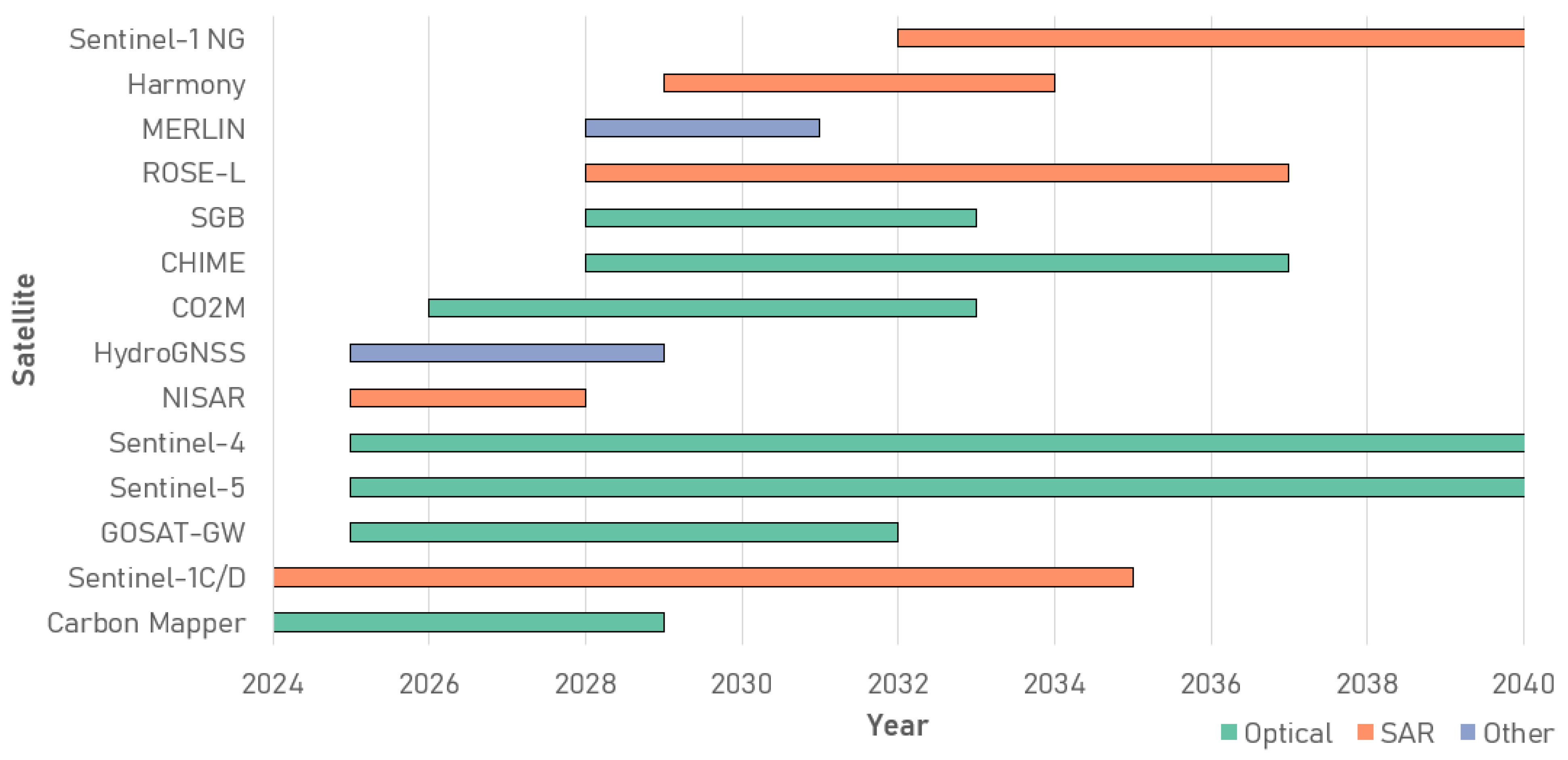
Recent and upcoming EO satellite missions (Figure 2) expand methane monitoring capacity across Arctic–boreal regions by addressing key physical observational constraints at high latitudes, including persistent cloud cover, polar darkness, and low solar angles. These missions improve capacity for addressing these issues through improved spatial resolution and temporal coverage to increase opportunities for cloud-free acquisitions, enhanced retrieval sensitivity under challenging illumination conditions, increasing coverage by active sensors that operate independently of solar illumination, and data continuity [55]. Active sensors such as MERLIN, ROSE-L, and NISAR do not require solar illumination, and missions such as GOSAT and CO2M offer improved revisit frequency and retrieval sensitivity. Several high-resolution optical missions, including Carbon Mapper, the Copernicus Hyperspectral Imaging Mission for the Environment (CHIME), GHGSat, and Spaceborne Gas Imaging Spectrometer (SGB), supply fine spatial and spectral detail. However, their narrow swaths limit the regional applications of wetlands [56]. Area-flux mappers such as the Greenhouse Gases Observing Satellite–Greenhouse gases and Water cycle (GOSAT-GW) [110] and Copernicus Anthropogenic CO₂ Monitoring (CO2M) [111] aim to provide global coverage with revisit intervals of three to five days, sub-nanometer spectral sampling, and expected methane sensitivity near 10 ppb. These missions may reduce persistent observation gaps in high-latitude regions and improve the stability of column retrievals [112].

Additional missions within the Sentinel program extend atmospheric composition monitoring. Sentinel-5 provides SWIR trace-gas retrievals, while the Meteorological Operational Satellite—Second Generation (MetOp-SG) constellation offers daily global coverage and sub-daily revisit at polar latitudes through a suite of meteorological and atmospheric composition instruments [114]. Sentinel-4, launched in 2025, supplies high-frequency ultraviolet, visible, and near-infrared (UV-VIS-NIR) observations over Europe and complements methane-relevant products from Sentinel-5 and Sentinel-5 Precursor (Sentinel-5P, TROPOMI). Several SAR missions strengthen bottom-up methane modeling. The Radar Observing System for Europe in L-band (ROSE-L) [115] and the NASA–ISRO Synthetic Aperture Radar mission (NISAR) [116] provide L-band and S-band data that resolve vegetation structure, freeze–thaw transitions, soil moisture, and surface deformation [98]. The Sentinel-1 Next Generation (NG) mission [117] extends continuity beyond 2032. Harmony, a constellation of passive C-band SAR satellites flying in formation with Sentinel-1, retrieves three-dimensional surface motion fields [118]. The Methane Remote Sensing LiDAR Mission (MERLIN) introduces integrated-path differential absorption (IPDA) LiDAR retrievals, with an expected methane accuracy of below 10 ppb [119]. The Hydrology Global Navigation Satellite System (HydroGNSS) mission contributes soil moisture, inundation, freeze–thaw, and biomass data via GNSS-R [120]. The combined use of these sensors with fused optical products such as the Harmonized Landsat–Sentinel-2 (HLS) dataset [121,122] and Planet Fusion Monitoring [123] may reduce cloud-related data gaps and improve temporal continuity across Arctic–boreal regions. These missions offer new geophysical constraints for hydrology, permafrost processes, wetland dynamics, and atmospheric methane retrieval, supporting more stable top-down inversion inputs and more accurate bottom-up model parameters.

Table 2. Summary of emerging EO missions relevant to methane monitoring in Arctic–boreal regions.

Mission	Orbit	Key Capability	Expected Methane-Related Value
Carbon Mapper, CHIME, GHGSat, SGB	Sun-synchronous	High-resolution optical and hyperspectral imagery	Local-scale detection, vegetation and surface characterization
GOSAT-GW	Sun-synchronous	Enhanced SWIR sampling for methane and water cycle	Improved methane column retrievals
CO2M	Sun-synchronous	Sub-nanometer SWIR sensitivity	Regional and global inversion support
Sentinel-5	Sun-synchronous	Daily SWIR trace-gas retrieval	Higher-frequency methane sampling
MetOp-SG	Sun-synchronous	Atmospheric composition and meteorology	Constraints for methane transport and bottom-up modeling
Sentinel-4	Sun-synchronous	High-frequency UV-VIS-NIR	Complements Sentinel-5 methane-related products
NISAR	Geostationary	Deformation, freeze–thaw, soil moisture	Hydrology and permafrost inputs for bottom-up models
ROSE-L	Sun-synchronous	Vegetation structure, wetland extent	Improved mapping of wetland and lake dynamics
Harmony	Formation with Sentinel-1	3-D motion fields	Permafrost deformation and lake-ice dynamics
MERLIN	Sun-synchronous	IPDA LiDAR methane retrieval	High-accuracy methane columns (<10 ppb)
HydroGNSS	Sun-synchronous	Soil moisture, inundation, freeze–thaw via GNSS-R	Hydrological constraints for wetland and lake modeling
HLS	Sun-synchronous	30 m fused optical reflectance	Better optical continuity in cloudy regions
Planet	Sun-synchronous	Daily gap-free reflectance product	Higher temporal coverage for land-surface dynamics

summarizes the main EO missions relevant to upcoming methane monitoring efforts.

3. Bottom-Up Techniques for Estimating Methane Emissions

Bottom-up techniques estimate methane emissions by integrating land cover datasets with methane flux measurements or process-based models to extrapolate emissions across regional scales [124]. In situ measurements collected by sensors are used to both calibrate and validate bottom-up estimates and constrain top-down inversion models. Methods for detecting methane near and around the ground are diverse and involve measuring methane flux from the atmosphere above or downwind of an emitter. Ground-based measurements provide site-level data for model calibration and validation but have limited spatial and temporal coverage, especially in Arctic–boreal regions, where accessibility and weather pose challenges. The development of regional and global flux networks helps to address this data limitation and accessibility [125]. These networks continue to rapidly expand, including into Arctic–boreal regions.

Table 3. Comparison of ground-based methods for monitoring methane emissions from wetland and lake ecosystems.

Feature	Chambers and Bubble Traps	Spectrometers	Flux Towers
Measurement Type	Enclosure-based flux	Column-integrated concentration	Vertical flux (turbulent transport)
Spatial Scale	Small plot (cm–m)	Site to regional (line of sight)	Ecosystem-scale (hundreds of meters)
Temporal Resolution	Low to high (sporadic manual samples or recurring auto-sampling)	High (for stationary)	High (sub-hourly to daily)
Disturbance to Site	Minimal to Moderate	None	Minimal
Ease of Deployment	Moderate	Moderate to high (TCCON requires infrastructure)	High logistical effort
Suitability for Arctic	Limited by access/weather	High precision, limited coverage	Limited coverage, weather-dependent
Use in Upscaling	Yes, with design	Validation and calibration	Yes, high value in modeling
Used in Validation	Yes	Yes (esp. for satellites)	Yes (esp. for satellite products)

summarizes the three primary ground-based methane monitoring methods: chambers, spectrometers, and flux towers. The comparison highlights their spatial and temporal coverage, measurement approaches, and suitability for monitoring Arctic–boreal wetlands and lakes.

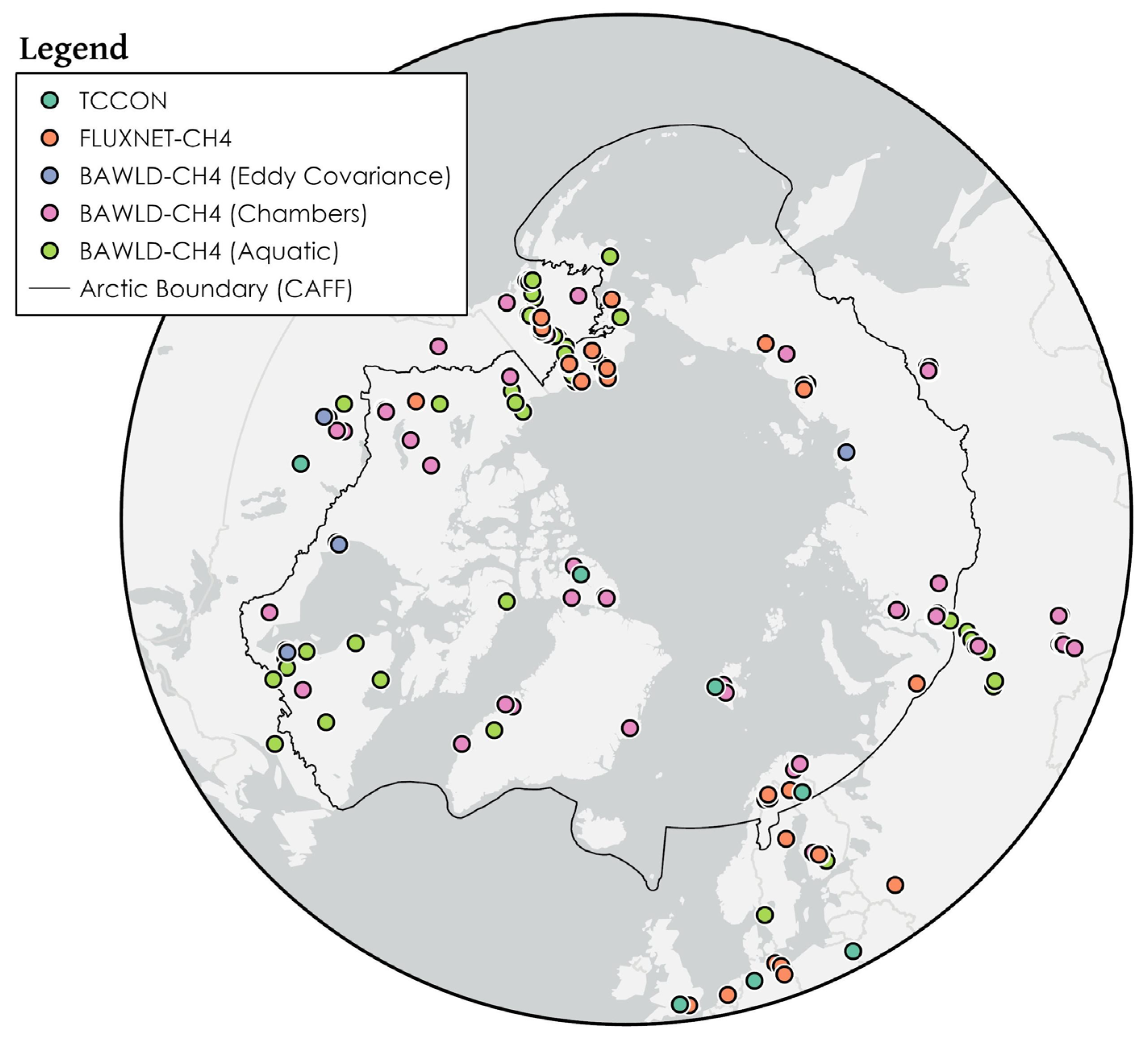
Figure 3 presents the distribution of key site-level methane measurement datasets across the region above 50°N, covering measurement sites with data from 2004 onward. This includes measurements derived from three major datasets: The Boreal Arctic Wetland and Lake Dataset Methane (BAWLD-CH4) [124], available through the National Science Foundation Arctic Data Center [126,127], FLUXNET-CH4 [125,128], available through the FLUXNET data portal [129], and Total Carbon Column Observing Network (TCCON) [130,131], available through the TCCON Data database [132]. The BAWLD-CH4 database covers both aquatic (e.g., lakes) and terrestrial (e.g., wetlands) methane flux observations and includes a variety of measurement techniques. Aquatic fluxes have been monitored at 259 Arctic sites using methods such as floating chambers and bubble traps, while terrestrial sites (wetlands) are primarily based on chamber measurements (82 sites) and a smaller subset of 11 sites using flux towers. The FLUXNET-CH4 network provides 32 Arctic sites with flux towers to measure net ecosystem methane fluxes, while TCCON contributes 8 Arctic stations based on high-precision column-integrated methane retrievals from ground-based Fourier-transform spectrometers.

3.1. Measurement Techniques for Ground-Based Methane Flux

One of the most common approaches for measuring methane flux is using static chambers. These chambers form an enclosure over a surface within which methane concentration is measured at once or over time to determine net flux in and out of that surface [133]. Chambers result in minimal ecosystem disturbance, useful for understanding environmental controls on methane at local scales. Transects and mobile chamber sampling can be used to observe patterns in methane flux across ecosystem units and landscapes. Extrapolation across large geographical and temporal scales should be done with careful consideration and experimental design [133,134,135,136]. While some chambers can detect ebullition, a more direct method is to use manual or automated bubble traps submerged in water or soil. Ebullition often exceeds diffusive methane release in lakes, particularly in Arctic–boreal landscapes where shallow waterbodies favor bubble transport [137].

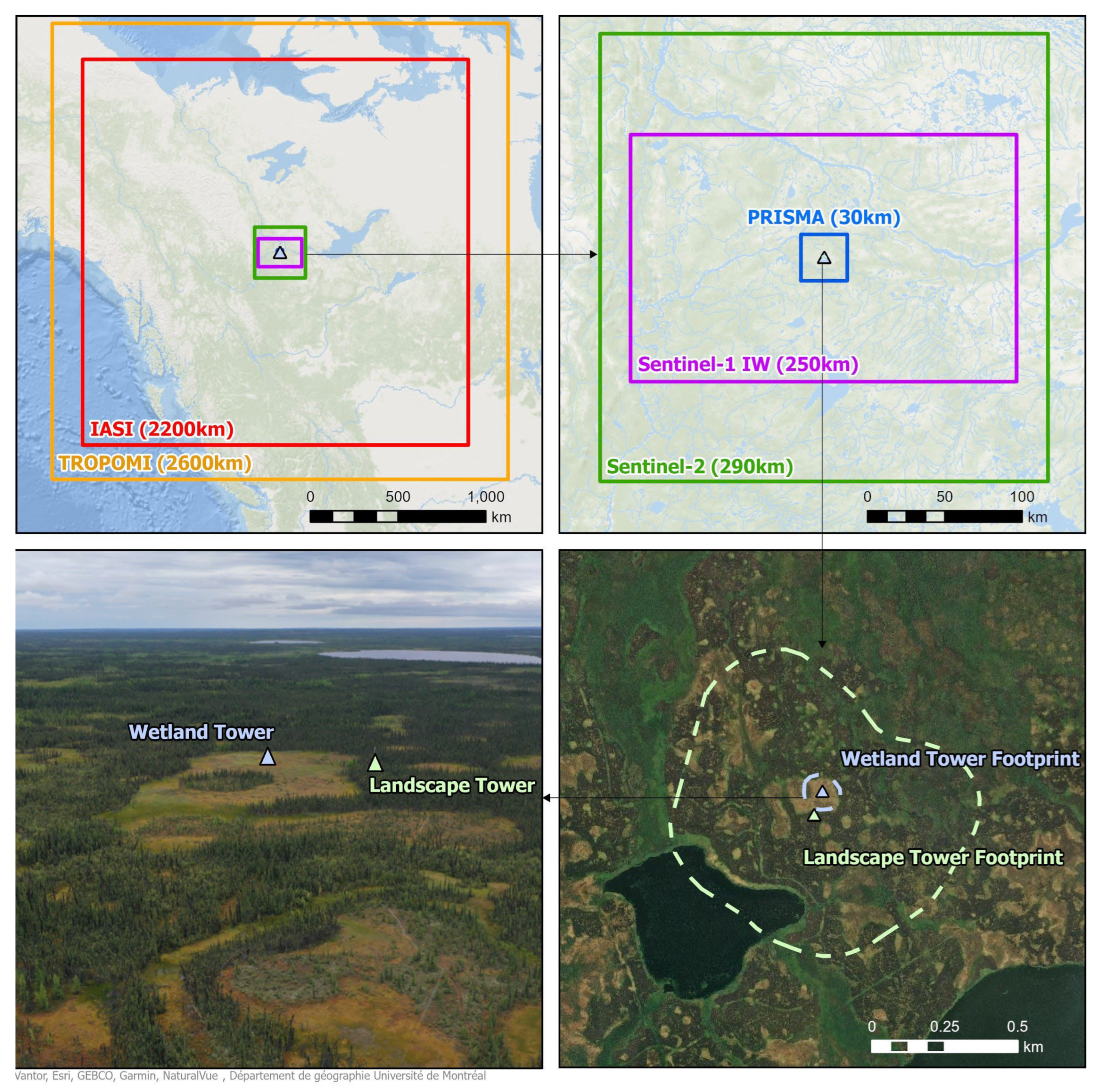
Measuring methane flux at the scale of hundreds of meters is possible using towers equipped with EC instrumentation [138]. EC Flux towers provide long-term, semi-continuous site-level flux data that is valuable for model calibration and validation [139]. High-frequency, continuous EC measurements are particularly valuable for capturing day-to-day variability in methane flux, which has been identified as a large source of uncertainty in annual emission estimates [140]. However, valid measurements require sufficient atmospheric turbulence. During stable night-time conditions or periods of poor weather, EC systems cannot produce reliable fluxes. Recent efforts have been made to better standardize measurements across these towers as demonstrated by the FLUXNET-CH4 network, established in 2019 [125]. FLUXNET-CH4 provides high-frequency, continuous methane flux measurements, capturing diurnal, seasonal, and interannual variations in methane emissions, and employs the EC method, a non-invasive technique that enables direct measurement of methane fluxes in natural ecosystems. This approach provides real-time insight into methane production and uptake dynamics. This dataset plays a key role in validating satellite-based methane retrievals and enhancing global methane monitoring efforts [125]. Despite its strengths, FLUXNET-CH4 has several limitations, particularly regarding spatial coverage (Figure 4). Additionally, the distribution of flux towers is uneven, with a bias towards high emission sites [45], introducing uncertainties in estimating the Arctic–boreal methane budget, where methane emissions are expected to rise due to permafrost thaw and wetland expansion (e.g., Schuur et al. [15]).

Another class of ground-based systems relies on path-integrated absorption spectroscopy. Instruments such as tunable diode laser absorption spectroscopy quantify methane concentration along a horizontal or slanted beam path and can resolve spatial differences across tens to hundreds of meters [136]. These systems fill an intermediate niche between chambers and flux towers by offering greater spatial coverage than chamber networks while still providing landscape-specific information. Although they do not measure flux directly, path-integrated instruments can support flux estimation when combined with wind information or mass-balance methods. Column-integrated spectrometers such as the TCCON do not fall within the bottom-up category because they measure the total atmospheric column rather than surface-attributable exchange. TCCON mainly supports satellite validation and long-term atmospheric monitoring [130,141,142,143,144].

3.2. EO and Inventory Maps

Structured inventories (

Table 4. Geospatial wetland and lake inventories that are frequently used in methane modeling.

Dataset	Spatial Resolution	Spatial Coverage	Temporal Coverage	Advantages	Limitations
HydroLAKES Messager et al. [92]	~500 m (15 arc-s)	Global	Static	Lake shorelines across the globe, with associated geometric and hydrological information. This dataset is integrated with additional hydrological datasets (HydroSHEDS, etc.).	Small waterbodies are underrepresented, limited temporal resolution, and issues around the accuracy of hydrological information.
GLOWABO Verpoorter et al. [146]	14.25 m	Global	Static	Extracts lakes globally using satellite imagery with associated geographical and morphometric characteristics.	Small waterbodies are underrepresented, and limited temporal resolution.
BAWLD Olefeldt et al. [126]	0.5° × 0.5° (~50 km at equator)	>50°N	Static	Classifies wetlands and lakes with a reported confidence interval, addressing issues related to double counting.	Small lakes contribute disproportionally to spatial uncertainty of lake area. The grid-based approach has limited utility for site-specific analysis.
WAD2M Zhang et al. [147]	0.25° × 0.25° (~25 km at equator)	Global	Monthly (2000–2018)	A time series of surface inundation with good agreement with existing wetland inventories.	Coarse resolution and excludes permanent water bodies and coastal wetlands with limited detection in dense vegetation.
GLWD Lehner et al. [12]	15 arc-s (~500 m)	Global	Static	Fractional coverage of wetlands and lakes allowing for multiple classes per grid cell, distinguishing between numerous wetland and waterbody classes.	Static map inheriting inaccuracies of multiple contributing datasets.
GIEMS-2 Prigent et al. [148]	0.25° × 0.25° (~25 km at equator)	Global	Monthly (1992–2020)	Long-term time series of surface water dynamics.	Coarse resolution dataset that overestimates classification results in low vegetation areas.
CCI Land Cover Copernicus Climate Change Service, Climate Data Store [149]	300 m	Global	Annual (1992–2022)	Annual land cover maps classified using a standardized classification framework developed by the United Nations Food and Agriculture Organization and designed to feed specifically into climate models	Coarse spatial resolution and wetland classification is not type-specific.
JRC Global Surface Water Pekel et al. [150]	30 m	Global	Monthly (1984–2021)	High-resolution detection of surface water extent and dynamics, and includes information on occurrence, seasonality, recurrence, and transitions	Significant data gaps (areas with no observations).
SWAMPS Jensen and Mcdonald [151]	0.25° × 0.25° (~25 km at equator)	Global	Daily (1992–2013+)	Daily time series of inundated area fraction, sensitive to surface water and vegetation structure	Coarse resolution, overestimation in arid regions, and cannot detect water under a closed forest canopy.

) provide foundational spatial data for methane flux estimation [24,54,145]. Although these inventories do not include direct methane flux measurements, they offer valuable environmental parameters (such as wetland extent, lake morphometry, surface hydrology, and land cover classification) that inform and improve bottom-up emission estimation approaches. These spatial layers are valuable for validating satellite-based retrievals and constraining process-based models. Most of these inventories are derived from satellite EO data, including optical imagery, active and passive microwave data, and multi-sensor fusion approaches, though some, including the Global Lakes and Wetlands Database (GWLD), are created through the harmonization of various existing datasets.

In addition to static inventories, EO-based mapping approaches offer dynamic and scalable tools for delineating Arctic–boreal wetland and lake ecosystems [10,152]. As a result, remote sensing technologies have become invaluable for mapping and monitoring large regional areas. To enhance the accuracy of wetland and lake classification, researchers are increasingly turning to machine learning and AI (e.g., [153]). Techniques such as object-based image analysis (OBIA) allow for more nuanced interpretation of remote sensing imagery by classifying regions or objects of interest rather than individual pixels [154,155]. By integrating multiple data sources, machine learning algorithms such as Random Forests, Support Vector Machines, Extreme Gradient Boosting, and deep learning models can enhance the classification of wetland and lake types by analyzing spectral, spatial, and temporal data [156,157]. The integration of machine learning techniques with multi-source remote sensing data has proven highly effective for Arctic–boreal ecosystems [158,159,160,161].

The integration of high-resolution satellite instrument data, such as Sentinel-1 (C-band), ALOS PALSAR-2 (L-band), and Sentinel-2, with machine learning classification techniques has significantly improved wetland and lake mapping accuracy in the Arctic–boreal region [61,162]. Nonetheless, several challenges remain, particularly the lack of consistent training data for Arctic–boreal ecosystems and the complexities of classifying highly dynamic landscapes. In particular, the overlap between wetlands and lakes, combined with seasonal variations in water levels and vegetation, complicates classification efforts. Additionally, in situ data, which is essential for validating remote sensing classifications, remains challenging in the Arctic–boreal region due to the remote nature of these ecosystems and the difficulty of conducting field surveys in vast, inaccessible regions.

3.3. Wetland Emission Modeling

Accurately estimating methane emissions from wetlands requires reliable modeling techniques that can scale field-based emission measurements to larger regions. Bottom-up approaches commonly integrate local flux data with broader environmental datasets, such as land cover information. These models typically fall into three main categories: empirical models, process-based models, and data-driven models [26]. While all three approaches leverage relationships between environmental factors and methane emissions, they differ in their underlying methodologies and assumptions.

3.3.1. Empirical and Data-Driven Modeling

Empirical and data-driven approaches estimate methane emissions by establishing statistical relationships between observed fluxes and environmental variables without explicitly simulating underlying biogeochemical processes. These methods are widely used for scaling local measurements to broader regions and perform well when sufficient observational data exist [26].

Traditional empirical models rely on predefined functional forms to represent first-order environmental controls such as soil hydrology, water table depth, and temperature. A prominent example is the global wetland methane emission framework developed by Bloom et al. [90], which integrates satellite-derived wetland extent and surface temperature. This work informed the WetCHARTs ensemble used in many atmospheric inversion systems. Empirical models often employ parameters such as Q10, which reflect the temperature sensitivity of methane emissions. However, Q10 values vary widely due to differences in site conditions and measurement protocols, which can introduce substantial uncertainty when these models are applied across diverse environments [163,164,165].

Data-driven approaches, which include machine learning techniques, extend empirical modeling by allowing more flexible representations of nonlinear relationships across large and heterogeneous datasets [166]. Rather than prescribing a specific equation, these models infer patterns directly from the data and do not impose prior assumptions about the underlying distribution of predictors or responses. Machine learning models integrate field measurements, land cover information, and environmental variables to generate scalable estimates of methane across wetland landscapes. For example, McNicol et al. [167] used a random forest algorithm to upscale FLUXNET-CH4 methane fluxes, while Yuan et al. [168] introduced a causality-guided framework that embeds mechanistic insights into the modeling pipeline to improve generalization in data-sparse Arctic–boreal regions.

Despite their strengths, empirical and data-driven models remain constrained by the availability and representativeness of ground measurements. Spatial biases, limited coverage in remote Arctic–boreal areas, and uncertainties in training data can influence model accuracy. Nonetheless, flexible empirical approaches remain essential components of bottom-up methane emission estimation frameworks, particularly when complemented by process-based models or physically informed constraints.

3.3.2. Process-Based Modeling

Process-based models are designed to simulate the fundamental biogeochemical mechanisms driving methane production in wetlands and lakes [169]. These models incorporate environmental factors such as temperature, soil moisture, and availability of organic matter to represent how methane is generated, oxidized, and transported under varying conditions. Unlike empirical models, they do not rely solely on statistical relationships but instead explicitly simulate physical, chemical, and biological processes, providing a mechanistic understanding of methane fluxes [170].

Process-based models typically resolve major methane pathways, including microbial production in saturated soils, oxidation in aerobic layers, and transport via diffusion, ebullition, and plant aerenchyma. A common approach within process-based modeling combines methane flux estimates (per unit area) with wetland inundation extent to calculate total methane emissions. Wetland extent can be derived from static or dynamic maps, remote sensing products, or hydrological models [26]. Such intercomparison studies have played a central role in global methane budget assessments [1,171].

3.4. Lake Modeling

While wetlands have received considerable attention and have been the subject of modeling efforts in the past few years, lakes remain a notable gap in methane emission modeling [47]. The current methodologies for upscaling lake emissions primarily rely on individual lake area data, which overlooks the complexities of methane production and emission within lakes [37]. Although some modeling efforts incorporate variables such as lake type and chlorophyll, area and temperature remain the most commonly used predictors [54]. Existing global lake inventories (Table 4) suffer from the significant omission of small lakes and ponds, which are prevalent in the Arctic–boreal landscape. Additionally, the role of aquatic vegetation in methane emissions from lakes has been largely overlooked [172]. One possible strategy to reduce the biases and uncertainties in lake methane flux estimation involves carefully selecting and testing the drivers used for upscaling [145]. For example, Deemer and Holgerson [173] employed a dataset [174] that broke down total, diffusive, and ebullitive methane emissions in different waterbodies to identify the best predictors for methane flux. Their findings underscore that the most effective parameters can vary by waterbody type, with morphometric variables such as surface area and maximum depth playing important roles in scaling up lake methane emissions.

Satellite-derived biophysical data offer an expanding set of spatial predictors for major lake emissions via diffusive and ebullitive pathways. Duan et al. [175], for example, demonstrated that chlorophyll a, water surface temperature, and light attenuation retrieved from MODIS can serve as inputs to a random forest model, enabling the reconstruction of an 18-year daily time series of diffusive methane flux in a eutrophic lake, illustrating how satellite observations can substitute for sparse in situ measurements that currently constrain upscaling efforts. Engram et al. [100] demonstrated that L-band SAR backscatter parameters acquired during ice-cover periods can capture the distortion of the ice–water interface caused by trapped ebullitive bubbles, enabling ebullition estimates across thousands of lakes simultaneously. These studies suggest that incorporating satellite-derived inputs into lake emission modeling frameworks can meaningfully expand the model predictor space beyond morphological and climate variables.

Hydrologic Modeling and Routing

Hydrological models are fundamental tools for studying the impact of hydrological changes on local, regional, and global catchment behavior, runoff variability [176,177], and methane emissions. Process-based hydrologic models can represent fundamental hydrologic mechanisms across complex Arctic–boreal lake-dominated landscapes. Such modeling must incorporate spatial and temporal variability of water table, active layer depth, soil moisture, soil temperature, snow cover, lake ice, lake area, lake drainage, and wetland conditions at a high spatial resolution.

Snow plays a key role in controlling many aspects of the Arctic–boreal hydrologic system [178], including lake ice cover, radiation penetration through the ice, ground temperature, and runoff. Therefore, accounting for snow processes is essential for understanding methane release. A novel update of Pomeroy et al. [178] modeling of Arctic–boreal snow is the Canadian Hydrological Model (CHM) [179]. CHM is a high-resolution, physics-based, variable-resolution model that allows modeling of snow cover on lakes and surrounding watersheds with high resolution at key landscape nodes. Snow output from CHM can be input to GEOtop, a high-resolution permafrost-hydrology model that includes key aspects of the hydrology of watersheds, including permafrost, surface energy balance, soil moisture, soil temperature, and runoff [180,181]. Other models useful for applications in complex Arctic–boreal regions include the Topographic Model (TOPMODEL) and the Soil and Water Assessment Tool (SWAT).

Satellite-derived data has an important role in the calibration of hydrological models and routing parameters, particularly within the context of monitoring Arctic–boreal wetlands, lakes, and permafrost freeze–thaw processes [182]. Integrating EO data with hydrological models to simulate water movement across landscapes can provide valuable insights into the factors driving wetland and lake dynamics in the region, which are critical for identifying critical areas where methane emissions are likely to occur and for understanding the factors influencing their release. Moreover, satellite data facilitates calibration of complex hydrological models by integrating data assimilation techniques that account for both model and observation errors. This approach enables more precise estimation of state variables, such as soil moisture and freeze/thaw states, essential for monitoring permafrost dynamics and wetland/lake interactions in Arctic–boreal environments [183].

4. Top-Down Techniques for Estimating Methane Emissions

Top-down approaches do not directly measure methane emissions. Instead, they retrieve atmospheric methane column concentrations from satellite or airborne observations and subsequently infer surface fluxes using atmospheric transport models and inverse modeling frameworks. These inversion systems combine observed methane enhancements with prior emission inventories and meteorological transport simulations to estimate the spatial distribution and magnitude of surface methane emissions.

While this framework has proven effective at constraining methane emissions at regional and global scales, attributing emissions to specific source types depends on the spatial resolution of observations, the accuracy of prior inventories, and the representation of atmospheric transport processes. Diffuse, spatially fragmented sources, such as small Arctic lakes, remain challenging to isolate using top-down approaches alone, as satellite footprints and boundary-layer mixing often aggregate emissions over large areas.

Satellite-based top-down systems retrieve methane column concentrations primarily using instruments operating in the SWIR absorption bands, while TIR instruments provide complementary vertical sensitivity. These approaches provide large-scale coverage and frequent observations, making them particularly valuable for monitoring expansive and remote areas such as Arctic–boreal ecosystems. Compared with bottom-up inventories, which can involve considerable spatial uncertainties, sporadic updates, and limited temporal coverage, top-down satellite instrument observations offer large-scale and frequent measurement opportunities [80,184]. Satellite instruments can provide data at global, regional, and local scales, enabling the monitoring of methane emissions from broad atmospheric patterns down to specific point sources [55].

Wetland methane emissions are typically mapped using area flux instruments that capture large-scale emissions, whereas point-source imagers are designed to detect localized plumes, such as those from oil and gas infrastructure. Given that wetland methane emissions are sparsely distributed, area flux mapping instruments are better suited to characterizing the spatial extent of these sources. Area flux mappers generally estimate methane columns at regional or global scales by applying inversion techniques to satellite instrument observations. For example, TROPOMI measures atmospheric methane at the 2.3 μm SWIR absorption band with a detection limit of around ∼5 t h⁻¹ under ideal conditions [86,185]. This provides a broad, top-down perspective of methane emissions. TIR instruments, such as the IASI, measure methane in the 7.7 μm band and have a spatial resolution of 1 km, collecting data from the mid- to upper troposphere [186,187].

Another method for retrieving methane columns is the carbon dioxide proxy approach, which leverages adjacent absorption features of carbon dioxide and methane in the 1.65 μm band [188,189,190]. This technique is particularly relevant for instruments such as GOSAT, which have only the 1.65 μm band available. The carbon dioxide proxy technique generally exhibits reduced sensitivity to surface and aerosol artifacts. However, it can be more prone to any biases in carbon dioxide columns, or if the same source emits both carbon dioxide and methane [55,83]. Moreover, retrievals at 1.65 μm are constrained by weaker methane absorption lines, potentially limiting sensitivity [55]. Despite these challenges, the GOSAT carbon dioxide proxy achieves a higher retrieval success rate, particularly in regions with high aerosol levels or thin clouds. This method achieves up to a 24% global success rate over land, compared to the roughly 3% success rate reported for TROPOMI inversions [83,190]. Nevertheless, GOSAT’s three-day revisit time, coarser spatial resolution, and widely spaced footprints (approximately 250 km apart) can limit its applicability to capture fine-scale or rapidly changing methane emissions [190].

The inversion techniques rely on forward atmospheric transport models to link satellite instrument observations with the methane column enhancement, optimizing this relationship through iterative adjustments. Goddard Earth Observing System—Chemistry (GEOS-Chem) is one of the most widely used atmospheric chemistry models for this purpose and is typically driven by assimilated meteorological datasets such as GEOS-FP (Goddard Earth Observing System—Forward Processing) and MERRA-2 (Modern-Era Retrospective analysis for Research and Applications, Version 2) [184,190]. By coupling these atmospheric models with satellite instrument measurements, the inversion framework refines prior emission estimates to produce a more accurate representation of methane fluxes. Bayesian inference is commonly employed to optimize inversion techniques, requiring a prior estimate of emissions to guide the solution [191]. Bottom-up methane inventories, which offer a solid initial estimate of methane columns, play a pivotal role here [192]. Sector-specific bottom-up datasets, such as the gridded United Nations Framework Convention on Climate Change (UNFCCC) [193] or Emissions Database for Global Atmospheric Research (EDGAR) inventories [194], provide initial estimates for anthropogenic sources (e.g., fossil fuels), while WetCHART is a frequently used prior inventory for wetland methane emissions [52,90]. These datasets are often used in combination to constrain inversion models, though they are associated with significant uncertainties [195]. Through iterative minimization of the cost function, the inversion framework aligns model-simulated methane columns with satellite-derived observations. This process enables improved estimation of near-real-time methane fluxes.

The Integrated Methane Inversion (IMI) offers significant advantages for inverse modeling and Arctic–boreal wetland and lake methane emission estimation, particularly in the challenging context of remote and hard-to-monitor regions [196]. By using satellite data from the TROPOMI instrument and blending it with GOSAT data, IMI 2.0 enhances the accuracy of methane emission estimates by correcting biases and improving data quality [197]. This blended approach, combined with the ability to incorporate point-source emissions data, provides a comprehensive tool for refining methane fluxes in regions where emissions are dynamic and difficult to quantify using traditional methods. IMI’s high spatial resolution (up to 0.25° × 0.3125°) and its ability to optimize methane emissions at various scales (from regional to global) are especially beneficial for capturing the unique dynamics of Arctic–boreal ecosystems, where methane fluxes fluctuate due to freeze–thaw cycles and other seasonal factors. Furthermore, the IMI enables continuous emission updates via a Kalman filter, enabling near-real-time monitoring of methane emissions. This capability is essential for tracking seasonal and interannual variability in emissions from Arctic–boreal wetlands and lakes, where methane release is highly sensitive to changing environmental conditions. The integration of improved error characterization, adaptive state-vector clustering, and boundary-condition optimization further strengthens IMI’s ability to provide reliable methane flux estimates for these critical ecosystems.

The potential of top-down inversion techniques to yield accurate posterior estimates of methane flux across multiple sectors, including wetlands, has been demonstrated in numerous studies [82,184]. These methods are commonly validated against ground-based measurements from the TCCON or via cross-comparisons with other satellite datasets, such as GOSAT. One notable advancement in this field is the development of the IMI framework, which facilitates methane column estimation for different scenarios and conditions by offering varied inversion configurations [83,196]. Recognizing that GOSAT retrievals often exhibit reduced biases, Balasus et al. [198] developed a blended TROPOMI–GOSAT methane product to refine TROPOMI observations, achieving reduced variable biases. By training machine learning models to capture systematic differences between TROPOMI and GOSAT measurements, bias corrections are applied to TROPOMI retrievals, yielding an enhanced methane column dataset. This blended product shows stronger agreement with TCCON observations than unadjusted TROPOMI data, thereby improving confidence in satellite-based top-down methane estimates.

Despite recent progress in top-down methane estimations for wetlands, several challenges persist, particularly for Arctic–boreal regions. One key limitation stems from the sparse coverage of satellite instrument observations at high latitudes, constrained by persistent cloud cover, low solar angles, and periods of extended darkness [55]. These limitations become more pronounced during winter, further reducing both EO opportunities and the feasibility of deriving methane column measurements from space-based instruments. Additionally, top-down inverse modeling in Arctic–boreal areas is hindered by limited atmospheric measurements, which restrict the precision of the derived flux estimates [199]. Uncertainties embedded within bottom-up inventories can also propagate through the inversion process, affecting the reliability of results. In particular, uneven or minimal data coverage over Arctic–boreal regions can bias the prior estimates used in forward models, ultimately skewing the final posterior emissions [200]. Addressing these challenges is pivotal for refining top-down assessments and achieving more accurate methane budgets in high-latitude ecosystems.

5. Knowledge Gaps

There remains a need for high-quality, accurate spatial data on wetland and lake distribution and dynamics that capture size, shape, and type, as well as inundation depth and duration. Ecosystems such as small lakes [201,202] and marsh wetlands [203] tend to be underestimated in large-geographical-scale datasets such as BAWLD-CH4 and the Canadian Wetland Inventory Map [61,126]. Additionally, waterbody spatial datasets fail to capture defining characteristics of lakes such as shape and size, substrate, and formation, which are tied to methane flux patterns [173,204,205]. Poor resolution of waterbody margins may be particularly detrimental, as these areas often function as methane emission hotspots [206,207]. Shoreline zones are typically shallow and receive high inputs of organic matter from both aquatic and terrestrial sources, creating carbon-rich sediments favorable for methanogenesis. Fluctuating water levels in these transitional environments promote alternating oxic and anoxic conditions, which can enhance microbial methane production while limiting sustained oxidation. In addition, emergent macrophytes common in near-shore areas provide conduits for plant-mediated methane transport, bypassing oxidation in the water column. Shallow depths also facilitate ebullition, as reduced hydrostatic pressure allows methane bubbles to escape more readily to the atmosphere. For example, accounting for shallow, vegetated near-shore areas in Arctic–boreal lakes has been shown to increase total lake methane emission estimates by approximately 21%, underscoring the sensitivity of upscaled flux calculations to shoreline representation [83].

Inundation is a major defining characteristic of seasonality and is a major driver of changes in methane emissions in both wetlands and lakes; however, a majority of wetland and lake geospatial datasets capture these ecosystems for only a snapshot in time [201,208]. These snapshots are typically captured during warmer seasons, resulting in a lack of information related to methane flux during seasons with limited sunlight [84,138]. The BAWLD-CH4 dataset, for example, has limitations in representing methane flux during the autumn and winter months. Seasonal variations in methane emissions from thermokarst lakes remain poorly understood, particularly during ice melt seasons [138]. Information about cold-season emissions is limited in the current process models [209]. Additionally, there remains a lack of consideration towards large-scale weather events such as El Niño [184] and how these events impact methane emission from different ecosystems, both immediately after the weather event, and how these events impact the vegetation and hydrology of the impacted ecosystems over the long term.

There are also significant gaps in the usability and integration of existing wetland and lake methane emission inventories. Many inventories differ in wetland classification schemes, spatial and temporal resolutions, and underlying methodological assumptions, making cross-comparison and integration difficult. Obstacles include inconsistent definitions of wetland types, limited representation of small and dynamic ecosystems, insufficient transparency in metadata, and a general lack of standardization across datasets. These inconsistencies introduce uncertainty when inventories are used for bottom-up methane modeling or when comparing them with satellite observations.

To improve usability, future inventories should prioritize standardized classification systems, higher spatial and temporal resolution, harmonized data structures, clear documentation of methodologies, and robust uncertainty quantification. Developing interoperable, harmonized wetland inventories would significantly enhance their value for estimating methane emissions and broader climate change studies.

Another key challenge in refining methane emission estimates is the uncertainty in model parameters used in bottom-up methane emission models. These models, which simulate methane flux based on environmental drivers, such as temperature, hydroperiod, and microbial communities, require calibration using ground-based observational data. However, current models struggle to account for the substantial variability across wetland types and regions, especially in remote areas. High-frequency methane data, such as that from FLUXNET-CH4, are valuable in providing real-time methane flux measurements that are critical for refining model parameters. Yet, challenges remain in calibrating models across diverse wetland ecosystems.

Satellite remote sensing plays an essential role in validating and constraining bottom-up methane emission estimates. Instruments like GOSAT and TROPOMI, while useful for providing regional methane data, face challenges, including coarse spatial resolution. To address these limitations, new satellites such as MethaneSAT and the upcoming MERLIN LiDAR will offer improved spatial resolution and precision, crucial for tracking methane emissions in wetlands. However, these instruments will still face challenges in capturing methane emissions from highly dynamic ecosystems, such as Arctic–boreal wetlands, where hydrological seasonality significantly affects methane fluxes. Expanding the scope of satellite observations to specifically target wetland emissions, and coupling these measurements with ground-based data, is necessary for more accurate quantification of surface methane fluxes, particularly in wetlands that have a disproportionate impact on global methane emissions.

Finally, there is a general bias in inventories towards high-emitting sites (sources of methane) and a relatively poor capture of sinks, as reported by Voigt et al. [210], noting that the mechanisms controlling methane consumption in dry soils are poorly constrained. Similarly, methane oxidation in the model developed by Zhuang et al. [7] is not based on the observed methane oxidation rate but rather on net lake emission data; the model still found that warming permafrost enhanced methane oxidation in lake water, acting as a sink.

The importance of understanding methane emissions from wetlands and lakes cannot be overstated, especially as these ecosystems are sensitive to climate change and play a key role in global carbon dynamics. In addition to mapping wetland inundation and improving model parameterization, it is essential to continue to improve the capacity of remote sensing technologies to monitor methane fluxes at high spatial and temporal resolutions. Integrating satellite data, in situ measurements, and machine learning models may allow for more accurate estimates of methane emissions and help track the impacts of climate change on wetland dynamics. By addressing these issues, we may significantly enhance our understanding of wetland and lake carbon dynamics and contribute to more effective climate change mitigation strategies.

6. Opportunities

To address current knowledge gaps, state-of-the-art EO data, advanced AI methods, the expanding network of in situ methane measurements, and engagement with the broader methane research community can support the development of more accurate estimates of wetland and lake emissions across the Arctic–boreal region. Producing reliable estimates of wetland and lake extent and dynamics from high-resolution EO imagery and well-tested AI models is essential for monitoring small lakes, reducing double-counting, and characterizing hydrological and ice-related conditions. These features are necessary for representing temperature- and saturation-driven sensitivities in methane emission and can be derived from SAR and GNSS-R techniques. These updated datasets, in combination with in situ data, can then be integrated into two complementary Explainable Artificial Intelligence (XAI) models, where XAI refers to machine-learning approaches that provide transparent and interpretable insights into how predictions are made [211,212].

The first XAI model would estimate total methane emissions from wetlands and lakes by integrating the newly developed wetland and lake extents, dynamic landscape features, in situ flux observations, and hydrological indicators derived from InSAR. Total methane flux incorporates multiple pathways, including diffusion, plant-mediated transport, and ebullition, and the dominant drivers can vary across ecosystem types. A general model is therefore useful for identifying broad emission patterns across wetlands and lakes. The second XAI model would focus specifically on methane emission via ebullition. Ebullition is episodic, threshold-driven, and highly nonlinear, and lake morphology, sediment properties, and pressure variations influence it. These characteristics differ from those of diffusive or plant-mediated fluxes, and a dedicated model enables clearer identification of ebullition-specific controls. This ebullition-focused model could utilize SAR data and object-based machine learning classification to detect bubble signatures at lake surfaces, in conjunction with in situ measurements.

Next, top-down inversion methane estimates can be further improved by integrating the outputs of these XAI models with blended Sentinel-5P TROPOMI and GOSAT methane products and physics-informed neural network (PINN) frameworks. Recent studies [213,214] have demonstrated the application of physics-informed machine learning approaches to thermal infrared retrievals, including IASI methane products, by embedding physical radiative transfer constraints within neural network architectures to improve vertical sensitivity and reduce retrieval biases. Building on these developments, integrating XAI-based bottom-up constraints with PINN-enhanced top-down methane retrievals may improve consistency between surface-attributable emissions and atmospheric column observations. The outputs of the newly developed models could then be compared with established inversion systems and used to refine regional methane baselines for Arctic–boreal monitoring.

Recent advances in geospatial foundational models, such as AlphaEarth Foundations (AEF), have the potential to address critical data gaps, data availability, and accessibility in the Arctic–boreal region, integrating spatial, temporal, and measurement contexts across multiple EO sources into a unified geospatial representation [215]. Additionally, AEF can generate maps over time by learning temporal patterns and relationships between observations, thereby capturing dynamic information [215]. Applications of AEF have demonstrated that machine learning models can leverage the said model to extend labeled dataset information beyond originating geographical regions, by training machine learning models using AEF information as input features and ground truth data as targets, allowing the model to predict labels in data-scarce regions [216]. The integration of AEF into methane emission and land cover classification workflows may enhance accuracy, reduce the need for costly ground-truth data collection, and reduce uncertainty by providing improved training data.

7. Conclusions

Methane emissions from Arctic–boreal wetlands and lakes are critical for understanding climate feedback in a rapidly warming region. This review synthesizes the current state of knowledge on the monitoring and modeling of methane emissions from these ecosystems, highlighting both advancements and persistent obstacles across bottom-up, top-down, and hybrid approaches. EO technologies have made notable progress, particularly through improvements in spatial resolution, enhanced spectral capabilities, and increased temporal coverage. New and upcoming satellite missions, including MERLIN, GOSAT-GW, MethaneSAT, and the next generation of SAR instruments, are expected to reduce key information gaps by providing more accurate, consistent, and year-round atmospheric and surface observations. Multi-sensor fusion of SWIR and TIR observations represents a potential research focus, enabling year-round Arctic coverage with TIR instruments providing diurnal retrievals that complement the high-sensitivity SWIR spectrometer retrievals during sunlit hours. Meanwhile, advances in modeling, including mechanistic process-based models, data-driven approaches, and emerging geospatial AI frameworks, offer opportunities to better capture the complexity of methane flux drivers and to improve regional-to-global estimates.

However, substantial challenges remain. Wetland and lake datasets still struggle with issues such as underrepresentation of small waterbodies, inconsistent wetland classification schemes, and limited temporal resolution. Observational gaps during winter months hinder year-round methane monitoring, particularly at high latitudes where seasonal dynamics play a critical role. Additionally, the limited spatial coverage of flux towers and the sparsity of in situ measurements continue to constrain the accuracy of bottom-up inventories. Discrepancies between top-down and bottom-up approaches, including biases, coarse atmospheric product resolution, and inconsistent priors, further complicate methane budget assessments. Addressing these limitations will require a coordinated approach that integrates multi-source EO data, improves field measurements, enhances inventory harmonization, and enhances modeling frameworks. This includes reconciling inconsistent wetland and lake classification schemes to reduce double-counting, and advanced modeling frameworks for improved detection of small waterbodies, undersampled winter emissions, and seasonal and short-term environmental dynamics.

Looking ahead, the convergence of satellite-based atmospheric retrievals and high-resolution data will reduce uncertainties in Arctic–boreal methane emissions. By leveraging emerging geospatial foundation models, new methane-sensitive satellite missions, and expanded field networks such as FLUXNET-CH4 and TCCON, the research community has an unprecedented opportunity to produce more accurate and spatially resolved methane flux estimates. Integration of lidar data from MERLIN will allow for direct methane column retrievals independent of daylight with reduced sensitivity to methane albedo, which is particularly valuable in snow-covered boreal regions. Due to the limited lidar spatial coverage, this data should be used in tandem with passive spectrometers. Improving radiative transfer and surface reflectance parameterizations in high-albedo snow and ice surfaces and advancing data-driven inversion approaches that better resolve spatially heterogenous Arctic–boreal methane sources should remain a focus of the research. Continued collaboration across disciplines, including remote sensing, atmospheric science, hydrology, biogeochemistry, and machine learning, will be essential to advance monitoring capabilities, improve model representation, and enhance our understanding of methane-climate feedbacks in these critical ecosystems.

References

1. Saunois, M.; Martinez, A.; Poulter, B.; Zhang, Z.; Raymond, P.; Regnier, P.; Canadell, J.G.; Jackson, R.B.; Patra, P.K.; Bousquet, P.; et al. Global Methane Budget 2000–2020. Earth Syst. Sci. Data 2025, 17, 1873–1958. [Google Scholar] [CrossRef]
2. Lan, X.; Thoning, K.W.; Dlugokencky, E.J. Trends in Globally-Averaged CH4, N2O, and SF6 Determined from NOAA Global Monitoring Laboratory Measurements; NOAA Global Monitoring Laboratory: Boulder, CO, USA, 2022. [CrossRef]
3. Turner, A.J.; Frankenberg, C.; Kort, E.A. Interpreting Contemporary Trends in Atmospheric Methane. Proc. Natl. Acad. Sci. USA 2019, 116, 2805–2813. [Google Scholar] [CrossRef]
4. Bridgham, S.D.; Cadillo-Quiroz, H.; Keller, J.K.; Zhuang, Q. Methane Emissions from Wetlands: Biogeochemical, Microbial, and Modeling Perspectives from Local to Global Scales. Glob. Change Biol. 2013, 19, 1325–1346. [Google Scholar] [CrossRef]
5. Saunois, M.; Stavert, A.R.; Poulter, B.; Bousquet, P.; Canadell, J.G.; Jackson, R.B.; Raymond, P.A.; Dlugokencky, E.J.; Houweling, S.; Patra, P.K.; et al. The Global Methane Budget 2000–2017. Earth Syst. Sci. Data 2020, 12, 1561–1623. [Google Scholar] [CrossRef]
6. Peng, S.; Lin, X.; Thompson, R.L.; Xi, Y.; Liu, G.; Hauglustaine, D.; Lan, X.; Poulter, B.; Ramonet, M.; Saunois, M.; et al. Wetland Emission and Atmospheric Sink Changes Explain Methane Growth in 2020. Nature 2022, 612, 477–482. [Google Scholar] [CrossRef]
7. Zhuang, Q.; Guo, M.; Melack, J.M.; Lan, X.; Tan, Z.; Oh, Y.; Leung, L.R. Current and Future Global Lake Methane Emissions: A Process-Based Modeling Analysis. JGR Biogeosci. 2023, 128, e2022JG007137. [Google Scholar] [CrossRef]
8. Cunha-Santino, M.B.D.; Bianchini Júnior, I. Reviewing the Organic Matter Processing by Wetlands. Acta Limnol. Bras. 2023, 35, e19. [Google Scholar] [CrossRef]
9. Avis, C.A.; Weaver, A.J.; Meissner, K.J. Reduction in Areal Extent of High-Latitude Wetlands in Response to Permafrost Thaw. Nat. Geosci. 2011, 4, 444–448. [Google Scholar] [CrossRef]
10. Kåresdotter, E.; Destouni, G.; Ghajarnia, N.; Hugelius, G.; Kalantari, Z. Mapping the Vulnerability of Arctic Wetlands to Global Warming. Earth’s Future 2021, 9, e2020EF001858. [Google Scholar] [CrossRef]
11. Bao, T.; Jia, G.; Xu, X. Weakening Greenhouse Gas Sink of Pristine Wetlands under Warming. Nat. Clim. Change 2023, 13, 462–469. [Google Scholar] [CrossRef]
12. Lehner, B.; Anand, M.; Fluet-Chouinard, E.; Tan, F.; Aires, F.; Allen, G.H.; Bousquet, P.; Canadell, J.G.; Davidson, N.; Ding, M.; et al. Mapping the World’s Inland Surface Waters: An Upgrade to the Global Lakes and Wetlands Database (GLWD V2). Earth Syst. Sci. Data 2025, 17, 2277–2329. [Google Scholar] [CrossRef]
13. Dean, J.F.; Middelburg, J.J.; Röckmann, T.; Aerts, R.; Blauw, L.G.; Egger, M.; Jetten, M.S.M.; De Jong, A.E.E.; Meisel, O.H.; Rasigraf, O.; et al. Methane Feedbacks to the Global Climate System in a Warmer World. Rev. Geophys. 2018, 56, 207–250. [Google Scholar] [CrossRef]
14. Rantanen, M.; Karpechko, A.Y.; Lipponen, A.; Nordling, K.; Hyvärinen, O.; Ruosteenoja, K.; Vihma, T.; Laaksonen, A. The Arctic Has Warmed Nearly Four Times Faster than the Globe since 1979. Commun. Earth Environ. 2022, 3, 168. [Google Scholar] [CrossRef]
15. Schuur, E.A.G.; McGuire, A.D.; Schädel, C.; Grosse, G.; Harden, J.W.; Hayes, D.J.; Hugelius, G.; Koven, C.D.; Kuhry, P.; Lawrence, D.M.; et al. Climate Change and the Permafrost Carbon Feedback. Nature 2015, 520, 171–179. [Google Scholar] [CrossRef]
16. McIntosh Marcek, H.A.; Lesack, L.F.W.; Orcutt, B.N.; Wheat, C.G.; Dallimore, S.R.; Geeves, K.; Lapham, L.L. Continuous Dynamics of Dissolved Methane Over 2 Years and Its Carbon Isotopes (δ13 C, Δ14 C) in a Small Arctic Lake in the Mackenzie Delta. JGR Biogeosci. 2021, 126, e2020JG006038. [Google Scholar] [CrossRef]
17. Thornton, B.F.; Wik, M.; Crill, P.M. Double-counting Challenges the Accuracy of High-latitude Methane Inventories. Geophys. Res. Lett. 2016, 43, 12569–12577. [Google Scholar] [CrossRef]
18. Walter Anthony, K.M.; Vas, D.A.; Brosius, L.; Chapin, F.S.; Zimov, S.A.; Zhuang, Q. Estimating Methane Emissions from Northern Lakes Using Ice-bubble Surveys. Limnol. Oceanogr. Methods 2010, 8, 592–609. [Google Scholar] [CrossRef]
19. Sø, J.S.; Martinsen, K.T.; Kragh, T.; Sand-Jensen, K. Ebullition Dominates High Methane Emissions Globally across All Lake Sizes. Biogeochemistry 2025, 168, 43. [Google Scholar] [CrossRef]
20. DelSontro, T.; Boutet, L.; St-Pierre, A.; Del Giorgio, P.A.; Prairie, Y.T. Methane Ebullition and Diffusion from Northern Ponds and Lakes Regulated by the Interaction between Temperature and System Productivity. Limnol. Oceanogr. 2016, 61, S62–S77. [Google Scholar] [CrossRef]
21. Żygadłowska, O.M.; Venetz, J.; Lenstra, W.K.; Van Helmond, N.A.G.M.; Klomp, R.; Röckmann, T.; Veraart, A.J.; Jetten, M.S.M.; Slomp, C.P. Ebullition Drives High Methane Emissions from a Eutrophic Coastal Basin. Geochim. Cosmochim. Acta 2024, 384, 1–13. [Google Scholar] [CrossRef]
22. Vonk, J.E.; Tank, S.E.; Bowden, W.B.; Laurion, I.; Vincent, W.F.; Alekseychik, P.; Amyot, M.; Billet, M.F.; Canário, J.; Cory, R.M.; et al. Reviews and Syntheses: Effects of Permafrost Thaw on Arctic Aquatic Ecosystems. Biogeosciences 2015, 12, 7129–7167. [Google Scholar] [CrossRef]
23. Dallimore, S.R.; Lapham, L.L.; Côté, M.M.; Bowen, R.; MacLeod, R.; McIntosh Marcek, H.A.; Wheat, C.G.; Collett, T.S. Source, Migration Pathways, and Atmospheric Release of Geologic Methane Associated With the Complex Permafrost Regimes of the Outer Mackenzie River Delta, Northwest Territories, Canada. JGR Earth Surf. 2024, 129, e2023JF007515. [Google Scholar] [CrossRef]
24. Yuan, K.; Li, F.; McNicol, G.; Chen, M.; Hoyt, A.; Knox, S.; Riley, W.J.; Jackson, R.; Zhu, Q. Boreal–Arctic Wetland Methane Emissions Modulated by Warming and Vegetation Activity. Nat. Clim. Change 2024, 14, 282–288. [Google Scholar] [CrossRef]
25. Miner, K.R.; Turetsky, M.R.; Malina, E.; Bartsch, A.; Tamminen, J.; McGuire, A.D.; Fix, A.; Sweeney, C.; Elder, C.D.; Miller, C.E. Permafrost Carbon Emissions in a Changing Arctic. Nat. Rev. Earth Environ. 2022, 3, 55–67. [Google Scholar] [CrossRef]
26. Zhu, Q.; Jacob, D.J.; Yuan, K.; Li, F.; Runkle, B.R.K.; Chen, M.; Bloom, A.A.; Poulter, B.; East, J.D.; Riley, W.J.; et al. Advancements and Opportunities to Improve Bottom–up Estimates of Global Wetland Methane Emissions. Environ. Res. Lett. 2025, 20, 023001. [Google Scholar] [CrossRef]
27. Cowardin, L.M.; Carter, V.; Golet, F.C.; LaRoe, E.T. Classification of Wetlands and Deepwater Habitats of the United States; Northern Prairie Wildlife Research Center: Jamestown, ND, USA, 1979.
28. National Wetlands Working Group. The Canadian Wetland Classification System, 2nd ed.; University of Waterloo: Waterloo, ON, USA, 1997. [Google Scholar]
29. Bengtsson, L.; Herschy, R.W.; Fairbridge, R.W. (Eds.) Encyclopedia of Lakes and Reservoirs; Encyclopedia of Earth Sciences Series; Springer: Dordrecht, The Netherlands, 2012; ISBN 978-1-4020-5616-1. [Google Scholar]
30. Richardson, D.C.; Holgerson, M.A.; Farragher, M.J.; Hoffman, K.K.; King, K.B.S.; Alfonso, M.B.; Andersen, M.R.; Cheruveil, K.S.; Coleman, K.A.; Farruggia, M.J.; et al. A Functional Definition to Distinguish Ponds from Lakes and Wetlands. Sci. Rep. 2022, 12, 10472. [Google Scholar] [CrossRef]
31. Morris, M.; Chew, C.; Reager, J.T.; Shah, R.; Zuffada, C. A Novel Approach to Monitoring Wetland Dynamics Using CYGNSS: Everglades Case Study. Remote Sens. Environ. 2019, 233, 111417. [Google Scholar] [CrossRef]
32. Kreplin, H.N.; Santos Ferreira, C.S.; Destouni, G.; Keesstra, S.D.; Salvati, L.; Kalantari, Z. Arctic Wetland System Dynamics under Climate Warming. WIREs Water 2021, 8, e1526. [Google Scholar] [CrossRef]
33. Huang, C.; Smith, L.C.; Kyzivat, E.D.; Fayne, J.V.; Ming, Y.; Spence, C. Tracking Transient Boreal Wetland Inundation with Sentinel-1 SAR: Peace-Athabasca Delta, Alberta and Yukon Flats, Alaska. GISci. Remote Sens. 2022, 59, 1767–1792. [Google Scholar] [CrossRef]
34. Yuan, S.; Liang, X.; Lin, T.; Chen, S.; Liu, R.; Wang, J.; Zhang, H.; Gong, P. A Comprehensive Review of Remote Sensing in Wetland Classification and Mapping. arXiv 2025, arXiv:2504.10842. [Google Scholar] [CrossRef]
35. Marsh, P.; Russell, M.; Pohl, S.; Haywood, H.; Onclin, C. Changes in Thaw Lake Drainage in the Western Canadian Arctic from 1950 to 2000. Hydrol. Process. 2009, 23, 145–158. [Google Scholar] [CrossRef]
36. Emmerton, C.A.; Lesack, L.F.W.; Marsh, P. Lake Abundance, Potential Water Storage, and Habitat Distribution in the Mackenzie River Delta, Western Canadian Arctic. Water Resour. Res. 2007, 43, 2006WR005139. [Google Scholar] [CrossRef]
37. Pi, X.; Luo, Q.; Feng, L.; Xu, Y.; Tang, J.; Liang, X.; Ma, E.; Cheng, R.; Fensholt, R.; Brandt, M.; et al. Mapping Global Lake Dynamics Reveals the Emerging Roles of Small Lakes. Nat. Commun. 2022, 13, 5777. [Google Scholar] [CrossRef]
38. Jacob, D.J.; Turner, A.J.; Maasakkers, J.D.; Sheng, J.; Sun, K.; Liu, X.; Chance, K.; Aben, I.; McKeever, J.; Frankenberg, C. Satellite Observations of Atmospheric Methane and Their Value for Quantifying Methane Emissions. Atmos. Chem. Phys. 2016, 16, 14371–14396. [Google Scholar] [CrossRef]
39. Ganesan, A.L.; Schwietzke, S.; Poulter, B.; Arnold, T.; Lan, X.; Rigby, M.; Vogel, F.R.; Van Der Werf, G.R.; Janssens-Maenhout, G.; Boesch, H.; et al. Advancing Scientific Understanding of the Global Methane Budget in Support of the Paris Agreement. Glob. Biogeochem. Cycles 2019, 33, 1475–1512. [Google Scholar] [CrossRef]
40. Baldocchi, D.D. How Eddy Covariance Flux Measurements Have Contributed to Our Understanding of Global Change Biology. Glob. Change Biol. 2020, 26, 242–260. [Google Scholar] [CrossRef]
41. Shahan, J.; Chu, H.; Windham-Myers, L.; Matsumura, M.; Carlin, J.; Eichelmann, E.; Stuart-Haentjens, E.; Bergamaschi, B.; Nakatsuka, K.; Sturtevant, C.; et al. Combining Eddy Covariance and Chamber Methods to Better Constrain CO2 and CH4 Fluxes Across a Heterogeneous Restored Tidal Wetland. JGR Biogeosci. 2022, 127, e2022JG007112. [Google Scholar] [CrossRef]
42. Jentzsch, K.; Männistö, E.; Marushchak, M.E.; Rettelbach, T.; Golde, L.; Korrensalo, A.; Hashemi, J.; Van Delden, L.; Tuittila, E.; Knoblauch, C.; et al. Seasonality in Diffusive Methane Emissions Differs Between Bog Microforms. Glob. Change Biol. 2025, 31, e70372. [Google Scholar] [CrossRef]
43. Subke, J.-A.; Kutzbach, L.; Risk, D. Soil Chamber Measurements. In Springer Handbook of Atmospheric Measurements; Foken, T., Ed.; Springer International Publishing: Cham, Switzerland, 2021; pp. 1603–1624. ISBN 978-3-030-52171-4. [Google Scholar]
44. Pallandt, M.M.T.A.; Kumar, J.; Mauritz, M.; Schuur, E.A.G.; Virkkala, A.-M.; Celis, G.; Hoffman, F.M.; Göckede, M. Representativeness Assessment of the Pan-Arctic Eddy Covariance Site Network and Optimized Future Enhancements. Biogeosciences 2022, 19, 559–583. [Google Scholar] [CrossRef]
45. Skeeter, J.; Christen, A.; Henry, G.H.R. Controls on Carbon Dioxide and Methane Fluxes from a Low-Center Polygonal Peatland in the Mackenzie River Delta, Northwest Territories. Arct. Sci. 2022, 8, 471–497. [Google Scholar] [CrossRef]
46. Jung, M.; Schwalm, C.; Migliavacca, M.; Walther, S.; Camps-Valls, G.; Koirala, S.; Anthoni, P.; Besnard, S.; Bodesheim, P.; Carvalhais, N.; et al. Scaling Carbon Fluxes from Eddy Covariance Sites to Globe: Synthesis and Evaluation of the FLUXCOM Approach. Biogeosciences 2020, 17, 1343–1365. [Google Scholar] [CrossRef]
47. Matthews, E.; Johnson, M.S.; Genovese, V.; Du, J.; Bastviken, D. Methane Emission from High Latitude Lakes: Methane-Centric Lake Classification and Satellite-Driven Annual Cycle of Emissions. Sci. Rep. 2020, 10, 12465. [Google Scholar] [CrossRef]
48. Albuhaisi, Y.A.Y.; Van Der Velde, Y.; De Jeu, R.; Zhang, Z.; Houweling, S. High-Resolution Estimation of Methane Emissions from Boreal and Pan-Arctic Wetlands Using Advanced Satellite Data. Remote Sens. 2023, 15, 3433. [Google Scholar] [CrossRef]
49. Mavrovic, A.; Sonnentag, O.; Lemmetyinen, J.; Baltzer, J.L.; Kinnard, C.; Roy, A. Reviews and Syntheses: Recent Advances in Microwave Remote Sensing in Support of Terrestrial Carbon Cycle Science in Arctic–Boreal Regions. Biogeosciences 2023, 20, 2941–2970. [Google Scholar] [CrossRef]
50. Zhang, Z.; Poulter, B.; Melton, J.R.; Riley, W.J.; Allen, G.H.; Beerling, D.J.; Bousquet, P.; Canadell, J.G.; Fluet-Chouinard, E.; Ciais, P.; et al. Ensemble Estimates of Global Wetland Methane Emissions over 2000–2020. Biogeosciences 2025, 22, 305–321. [Google Scholar] [CrossRef]
51. Savignano, M.J.; Kyzivat, E.D.; Smith, L.C.; Engram, M. Geospatial Analysis of Alaskan Lakes Indicates Wetland Fraction and Surface Water Area Are Useful Predictors of Methane Ebullition. Ann. Am. Assoc. Geogr. 2024, 114, 299–313. [Google Scholar] [CrossRef]
52. Solazzo, E.; Crippa, M.; Guizzardi, D.; Muntean, M.; Choulga, M.; Janssens-Maenhout, G. Uncertainties in the Emissions Database for Global Atmospheric Research (EDGAR) Emission Inventory of Greenhouse Gases. Atmos. Chem. Phys. 2021, 21, 5655–5683. [Google Scholar] [CrossRef]
53. Laurion, I.; Vincent, W.F.; MacIntyre, S.; Retamal, L.; Dupont, C.; Francus, P.; Pienitz, R. Variability in Greenhouse Gas Emissions from Permafrost Thaw Ponds. Limnol. Oceanogr. 2010, 55, 115–133. [Google Scholar] [CrossRef]
54. Kyzivat, E.D.; Smith, L.C. A Closer Look at the Effects of Lake Area, Aquatic Vegetation, and Double-Counted Wetlands on Pan-Arctic Lake Methane Emissions Estimates. Geophys. Res. Lett. 2023, 50, e2023GL104825. [Google Scholar] [CrossRef]
55. Jacob, D.J.; Varon, D.J.; Cusworth, D.H.; Dennison, P.E.; Frankenberg, C.; Gautam, R.; Guanter, L.; Kelley, J.; McKeever, J.; Ott, L.E.; et al. Quantifying Methane Emissions from the Global Scale down to Point Sources Using Satellite Observations of Atmospheric Methane. Atmos. Chem. Phys. 2022, 22, 9617–9646. [Google Scholar] [CrossRef]
56. Mohammadimanesh, F.; Mahdianpari, M.; Radman, A.; Varon, D.; Hemati, M.; Marjani, M. Advancements in Satellite-Based Methane Point Source Monitoring: A Systematic Review. ISPRS J. Photogramm. Remote Sens. 2025, 224, 94–112. [Google Scholar] [CrossRef]
57. Conservation of Arctic Flora and Fauna High and Low Arctic Terrestrial Boundaries Were Defined by the Circumpolar Arctic Vegetation Mapping Project—Bioclimatic Subzones (CAVM). Sub Arctic Boundary Was Defined by the Arctic Biodiversity Assessment (ABA). 2001. Available online: https://statics.teams.cdn.office.net/evergreen-assets/safelinks/2/atp-safelinks.html (accessed on 11 March 2026).
58. Rouet-Leduc, B.; Hulbert, C. Automatic Detection of Methane Emissions in Multispectral Satellite Imagery Using a Vision Transformer. Nat. Commun. 2024, 15, 3801. [Google Scholar] [CrossRef]
59. Zortea, M.; De Sousa Almeida, J.L.; Klein, L.; Nogueira Junior, A.C. Detection of Methane Plumes Using Sentinel-2 Satellite Images and Deep Neural Networks Trained on Synthetically Created Label Data. In Proceedings of the 2023 IEEE International Conference on Big Data (BigData); IEEE: Sorrento, Italy, 2023; pp. 3830–3839. [Google Scholar]
60. Varon, D.J.; Jervis, D.; McKeever, J.; Spence, I.; Gains, D.; Jacob, D.J. High-Frequency Monitoring of Anomalous Methane Point Sources with Multispectral Sentinel-2 Satellite Observations. Atmos. Meas. Tech. 2021, 14, 2771–2785. [Google Scholar] [CrossRef]
61. Mahdianpari, M.; Brisco, B.; Granger, J.; Mohammadimanesh, F.; Salehi, B.; Homayouni, S.; Bourgeau-Chavez, L. The Third Generation of Pan-Canadian Wetland Map at 10 m Resolution Using Multisource Earth Observation Data on Cloud Computing Platform. IEEE J. Sel. Top. Appl. Earth Obs. Remote Sens. 2021, 14, 8789–8803. [Google Scholar] [CrossRef]
62. Hosseiny, B.; Mahdianpari, M.; Brisco, B.; Mohammadimanesh, F.; Salehi, B. WetNet: A Spatial–Temporal Ensemble Deep Learning Model for Wetland Classification Using Sentinel-1 and Sentinel-2. IEEE Trans. Geosci. Remote Sens. 2022, 60, 4406014. [Google Scholar] [CrossRef]
63. Marjani, M.; Mahdianpari, M.; Mohammadimanesh, F.; Gill, E.W. CVTNet: A Fusion of Convolutional Neural Networks and Vision Transformer for Wetland Mapping Using Sentinel-1 and Sentinel-2 Satellite Data. Remote Sens. 2024, 16, 2427. [Google Scholar] [CrossRef]
64. Marjani, M.; Mohammadimanesh, F.; Mahdianpari, M.; Gill, E.W. A Novel Spatio-Temporal Vision Transformer Model for Improving Wetland Mapping Using Multi-Seasonal Sentinel Data. Remote Sens. Appl. Soc. Environ. 2025, 37, 101401. [Google Scholar] [CrossRef]
65. Ingle, R.; Habib, W.; Connolly, J.; McCorry, M.; Barry, S.; Saunders, M. Upscaling Methane Fluxes from Peatlands across a Drainage Gradient in Ireland Using PlanetScope Imagery and Machine Learning Tools. Sci. Rep. 2023, 13, 11997. [Google Scholar] [CrossRef]
66. Guanter, L.; Irakulis-Loitxate, I.; Gorroño, J.; Sánchez-García, E.; Cusworth, D.H.; Varon, D.J.; Cogliati, S.; Colombo, R. Mapping Methane Point Emissions with the PRISMA Spaceborne Imaging Spectrometer. Remote Sens. Environ. 2021, 265, 112671. [Google Scholar] [CrossRef]
67. Marjani, M.; Mohammadimanesh, F.; Varon, D.J.; Radman, A.; Mahdianpari, M. PRISMethaNet: A Novel Deep Learning Model for Landfill Methane Detection Using PRISMA Satellite Data. ISPRS J. Photogramm. Remote Sens. 2024, 218, 802–818. [Google Scholar] [CrossRef]
68. Roger, J.; Irakulis-Loitxate, I.; Valverde, A.; Gorroño, J.; Chabrillat, S.; Brell, M.; Guanter, L. High-Resolution Methane Mapping With the EnMAP Satellite Imaging Spectroscopy Mission. IEEE Trans. Geosci. Remote Sens. 2024, 62, 4102012. [Google Scholar] [CrossRef]
69. Ouerghi, E.; Ehret, T.; Facciolo, G.; Meinhardt, E.; Marion, R.; Morel, J.-M. Tightening up Methane Plume Source Rate Estimation in EnMAP and PRISMA Images. Atmos. Meas. Tech. 2025, 18, 4611–4629. [Google Scholar] [CrossRef]
70. Ramsey, E., III; Rangoonwala, A. Hyperspectral Remote Sensing of Wetland Vegetation. In Advanced Applications in Remote Sensing of Agricultural Crops and Natural Vegetation; CRC Press: Boca Raton, FL, USA, 2018; pp. 219–248. [Google Scholar]
71. Jambhali, K.V.; Koirala, B.; Bnoulkacem, Z.; Scheunders, P. Soil Moisture Content Estimation From Hyperspectral Remote Sensing Data. IEEE J. Sel. Top. Appl. Earth Obs. Remote Sens. 2025, 18, 22231–22240. [Google Scholar] [CrossRef]
72. Fabbretto, A.; Pellegrino, A.; Giardino, C.; Bresciani, M.; Alikas, K.; Braga, F.; Vaičiūtė, D.; Lima, T.M.A.D.; Mangano, S.; Ghirardi, N.; et al. Hyperspectral Prisma Data Processing For Water Quality Research And Applications. In Proceedings of the IGARSS 2023—2023 IEEE International Geoscience and Remote Sensing Symposium; IEEE: Pasadena, CA, USA, 2023; pp. 1744–1747. [Google Scholar]
73. Cristóbal, J.; Graham, P.; Prakash, A.; Buchhorn, M.; Gens, R.; Guldager, N.; Bertram, M. Airborne Hyperspectral Data Acquisition and Processing in the Arctic: A Pilot Study Using the Hyspex Imaging Spectrometer for Wetland Mapping. Remote Sens. 2021, 13, 1178. [Google Scholar] [CrossRef]
74. Du, B.; Mao, D.; Wang, Z.; Qiu, Z.; Yan, H.; Feng, K.; Zhang, Z. Mapping Wetland Plant Communities Using Unmanned Aerial Vehicle Hyperspectral Imagery by Comparing Object/Pixel-Based Classifications Combining Multiple Machine-Learning Algorithms. IEEE J. Sel. Top. Appl. Earth Obs. Remote Sens. 2021, 14, 8249–8258. [Google Scholar] [CrossRef]
75. Huang, Y.; Peng, J.; Chen, N.; Sun, W.; Du, Q.; Ren, K.; Huang, K. Cross-Scene Wetland Mapping on Hyperspectral Remote Sensing Images Using Adversarial Domain Adaptation Network. ISPRS J. Photogramm. Remote Sens. 2023, 203, 37–54. [Google Scholar] [CrossRef]
76. Zhuo, W.; Wu, N.; Shi, R.; Liu, P.; Zhang, C.; Fu, X.; Cui, Y. Aboveground Biomass Retrieval of Wetland Vegetation at the Species Level Using UAV Hyperspectral Imagery and Machine Learning. Ecol. Indic. 2024, 166, 112365. [Google Scholar] [CrossRef]
77. Guanter, L.; Kaufmann, H.; Segl, K.; Foerster, S.; Rogass, C.; Chabrillat, S.; Kuester, T.; Hollstein, A.; Rossner, G.; Chlebek, C.; et al. The EnMAP Spaceborne Imaging Spectroscopy Mission for Earth Observation. Remote Sens. 2015, 7, 8830–8857. [Google Scholar] [CrossRef]
78. Transon, J.; D’Andrimont, R.; Maugnard, A.; Defourny, P. Survey of Hyperspectral Earth Observation Applications from Space in the Sentinel-2 Context. Remote Sens. 2018, 10, 157. [Google Scholar] [CrossRef]
79. Frankenberg, C.; Meirink, J.F.; Van Weele, M.; Platt, U.; Wagner, T. Assessing Methane Emissions from Global Space-Borne Observations. Science 2005, 308, 1010–1014. [Google Scholar] [CrossRef]
80. Irakulis-Loitxate, I.; Guanter, L.; Maasakkers, J.D.; Zavala-Araiza, D.; Aben, I. Satellites Detect Abatable Super-Emissions in One of the World’s Largest Methane Hotspot Regions. Environ. Sci. Technol. 2022, 56, 2143–2152. [Google Scholar] [CrossRef]
81. Shaw, J.T.; Allen, G.; Barker, P.; Pitt, J.R.; Pasternak, D.; Bauguitte, S.J.-B.; Lee, J.; Bower, K.N.; Daly, M.C.; Lunt, M.F.; et al. Large Methane Emission Fluxes Observed From Tropical Wetlands in Zambia. Glob. Biogeochem. Cycles 2022, 36, e2021GB007261. [Google Scholar] [CrossRef]
82. Albuhaisi, Y.A.Y.; Van Der Velde, Y.; Pandey, S.; Houweling, S. Integrating Satellite Observations and Hydrological Models to Unravel Large TROPOMI Methane Emissions in South Sudan Wetlands. Remote Sens. 2024, 16, 4744. [Google Scholar] [CrossRef]
83. Hancock, S.E.; Jacob, D.; Chen, Z.; Nesser, H.; Davitt, A.; Varon, D.J.; Sulprizio, M.P.; Balasus, N.; Estrada, L.A.; East, J.D.; et al. Satellite Quantification of Methane Emissions from South American Countries: A High-Resolution Inversion of TROPOMI and GOSAT Observations. Atmos. Chem. Phys. 2025, 25, 797–817. [Google Scholar] [CrossRef]
84. Li, M.; Kort, E.A.; Bloom, A.A.; Wu, D.; Plant, G.; Gerlein-Safdi, C.; Pu, T. Underestimated Dry Season Methane Emissions from Wetlands in the Pantanal. Environ. Sci. Technol. 2024, 58, 3278–3287. [Google Scholar] [CrossRef]
85. Liu, M.; Van Der, A.R.; Liu, R.; Van Weele, M.; Zhang, G.; De Laat, J.; Veefkind, P. Using TROPOMI Observations to Derive Methane Emissions and Its Driving Factors over Lake Chad. In Proceedings of the European Geosciences Union General Assembly 2024 (EGU24), Vienna, Austria, 14–19 April 2024. [Google Scholar]
86. Schuit, B.J.; Maasakkers, J.D.; Bijl, P.; Mahapatra, G.; Van Den Berg, A.-W.; Pandey, S.; Lorente, A.; Borsdorff, T.; Houweling, S.; Varon, D.J.; et al. Automated Detection and Monitoring of Methane Super-Emitters Using Satellite Data. Atmos. Chem. Phys. 2023, 23, 9071–9098. [Google Scholar] [CrossRef]
87. Lindqvist, H.; Kivimäki, E.; Häkkilä, T.; Tsuruta, A.; Schneising, O.; Buchwitz, M.; Lorente, A.; Martinez Velarte, M.; Borsdorff, T.; Alberti, C.; et al. Evaluation of Sentinel-5P TROPOMI Methane Observations at Northern High Latitudes. Remote Sens. 2024, 16, 2979. [Google Scholar] [CrossRef]
88. Japan Aerospace Exploration Agency. GOSAT/IBUKI-2 Data Users Handbook, 1st ed.; Japan Aerospace Exploration Agency: Tsukuba, Japan, 2020.
89. European Space Agency. Earth Online GOSAT-2; European Space Agency: Paris, Frence, 2025. [Google Scholar]
90. Bloom, A.A.; Bowman, K.W.; Lee, M.; Turner, A.J.; Schroeder, R.; Worden, J.R.; Weidner, R.; McDonald, K.C.; Jacob, D.J. A Global Wetland Methane Emissions and Uncertainty Dataset for Atmospheric Chemical Transport Models (WetCHARTs Version 1.0). Geosci. Model Dev. 2017, 10, 2141–2156. [Google Scholar] [CrossRef]
91. Bloom, A.A.; Bowman, K.W.; Lee, M.; Turner, A.J.; Schroeder, R.; Worden, J.R.; Weidner, R.J.; McDonald, K.C.; Jacob, D.J. CMS: Global 0.5-Deg Wetland Methane Emissions and Uncertainty (WetCHARTs v1.3.3); ORNL Distributed Active Archive Center: Oak Ridge, TN, USA, 2024. [CrossRef]
92. Messager, M.L.; Lehner, B.; Grill, G.; Nedeva, I.; Schmitt, O. Estimating the Volume and Age of Water Stored in Global Lakes Using a Geo-Statistical Approach. Nat. Commun. 2016, 7, 13603. [Google Scholar] [CrossRef]
93. Zhou, L.; Warner, J.; Nalli, N.R.; Wei, Z.; Oh, Y.; Bruhwiler, L.; Liu, X.; Divakarla, M.; Pryor, K.; Kalluri, S.; et al. Spatiotemporal Variability of Global Atmospheric Methane Observed from Two Decades of Satellite Hyperspectral Infrared Sounders. Remote Sens. 2023, 15, 2992. [Google Scholar] [CrossRef]
94. Schneider, M.; Ertl, B.; Diekmann, C.J.; Khosrawi, F.; Weber, A.; Hase, F.; Höpfner, M.; García, O.E.; Sepúlveda, E.; Kinnison, D. Design and Description of the MUSICA IASI Full Retrieval Product. Earth Syst. Sci. Data 2022, 14, 709–742. [Google Scholar] [CrossRef]
95. Fischer, H.; Birk, M.; Blom, C.; Carli, B.; Carlotti, M.; Von Clarmann, T.; Delbouille, L.; Dudhia, A.; Ehhalt, D.; Endemann, M.; et al. MIPAS: An Instrument for Atmospheric and Climate Research. Atmos. Chem. Phys. 2008, 8, 2151–2188. [Google Scholar] [CrossRef]
96. De Wachter, E.; Kumps, N.; Vandaele, A.C.; Langerock, B.; De Mazière, M. Retrieval and Validation of MetOp/IASI Methane. Atmos. Meas. Tech. 2017, 10, 4623–4638. [Google Scholar] [CrossRef]
97. Di Gioacchino, T.; Clarisse, L.; Noppen, L.; Van Damme, M.; Bauduin, S.; Coheur, P. Spatial and Temporal Variations of Thermal Contrast in the Planetary Boundary Layer. J. Remote Sens. 2024, 4, 0142. [Google Scholar] [CrossRef]
98. Adeli, S.; Salehi, B.; Mahdianpari, M.; Quackenbush, L.J.; Brisco, B.; Tamiminia, H.; Shaw, S. Wetland Monitoring Using SAR Data: A Meta-Analysis and Comprehensive Review. Remote Sens. 2020, 12, 2190. [Google Scholar] [CrossRef]
99. De La Barreda-Bautista, B.; Boyd, D.S.; Ledger, M.; Siewert, M.B.; Chandler, C.; Bradley, A.V.; Gee, D.; Large, D.J.; Olofsson, J.; Sowter, A.; et al. Towards a Monitoring Approach for Understanding Permafrost Degradation and Linked Subsidence in Arctic Peatlands. Remote Sens. 2022, 14, 444. [Google Scholar] [CrossRef]
100. Engram, M.; Walter Anthony, K.M.; Sachs, T.; Kohnert, K.; Serafimovich, A.; Grosse, G.; Meyer, F.J. Remote Sensing Northern Lake Methane Ebullition. Nat. Clim. Change 2020, 10, 511–517. [Google Scholar] [CrossRef]
101. Pointner, G.; Bartsch, A.; Dvornikov, Y.A.; Kouraev, A.V. Mapping Potential Signs of Gas Emissions in Ice of Lake Neyto, Yamal, Russia, Using Synthetic Aperture Radar and Multispectral Remote Sensing Data. Cryosphere 2021, 15, 1907–1929. [Google Scholar] [CrossRef]
102. Mohammadimanesh, F.; Salehi, B.; Mahdianpari, M.; Brisco, B.; Motagh, M. Wetland Water Level Monitoring Using Interferometric Synthetic Aperture Radar (InSAR): A Review. Can. J. Remote Sens. 2018, 44, 247–262. [Google Scholar] [CrossRef]
103. Hrysiewicz, A.; Williamson, J.; Evans, C.D.; Jovani-Sancho, A.J.; Callaghan, N.; Lyons, J.; White, J.; Kowalska, J.; Menichino, N.; Holohan, E.P. Estimation and Validation of InSAR-Derived Surface Displacements at Temperate Raised Peatlands. Remote Sens. Environ. 2024, 311, 114232. [Google Scholar] [CrossRef]
104. Tsokas, A.; Rysz, M.; Pardalos, P.M.; Dipple, K. SAR Data Applications in Earth Observation: An Overview. Expert Syst. Appl. 2022, 205, 117342. [Google Scholar] [CrossRef]
105. Mahdianpari, M.; Granger, J.E.; Mohammadimanesh, F.; Salehi, B.; Brisco, B.; Homayouni, S.; Gill, E.; Huberty, B.; Lang, M. Meta-Analysis of Wetland Classification Using Remote Sensing: A Systematic Review of a 40-Year Trend in North America. Remote Sens. 2020, 12, 1882. [Google Scholar] [CrossRef]
106. Chen, Z.; Banks, S.; Behnamian, A.; White, L.; Montpetit, B.; Pasher, J.; Duffe, J. Characterizing the Great Lakes Coastal Wetlands with InSAR Observations from X-, C-, and L-Band Sensors. Can. J. Remote Sens. 2020, 46, 765–783. [Google Scholar] [CrossRef]
107. Ledger, M.J.; Sowter, A.; Morrison, K.; Evans, C.D.; Large, D.J.; Athab, A.; Gee, D.; Brown, C.; Sjögersten, S. Potential of APSIS-InSAR for Measuring Surface Oscillations of Tropical Peatlands. PLoS ONE 2024, 19, e0298939. [Google Scholar] [CrossRef]
108. Mahdianpari, M.; Salehi, B.; Mohammadimanesh, F.; Motagh, M. Random Forest Wetland Classification Using ALOS-2 L-Band, RADARSAT-2 C-Band, and TerraSAR-X Imagery. ISPRS J. Photogramm. Remote Sens. 2017, 130, 13–31. [Google Scholar] [CrossRef]
109. Cohen, J.; Lemmetyinen, J.; Jorge Ruiz, J.; Rautiainen, K.; Ikonen, J.; Kontu, A.; Pulliainen, J. Detection of Soil and Canopy Freeze/Thaw State in the Boreal Region with L and C Band Synthetic Aperture Radar. Remote Sens. Environ. 2024, 305, 114102. [Google Scholar] [CrossRef]
110. Tanimoto, H.; Matsunaga, T.; Someya, Y.; Fujinawa, T.; Ohyama, H.; Morino, I.; Yashiro, H.; Sugita, T.; Inomata, S.; Müller, A.; et al. The Greenhouse Gas Observation Mission with Global Observing SATellite for Greenhouse Gases and Water Cycle (GOSAT-GW): Objectives, Conceptual Framework and Scientific Contributions. Prog. Earth Planet. Sci. 2025, 12, 8. [Google Scholar] [CrossRef]
111. Sierk, B.; Fernandez, V.; Bézy, J.-L.; Meijer, Y.; Durand, Y.; Bazalgette Courrèges-Lacoste, G.; Pachot, C.; Löscher, A.; Nett, H.; Minoglou, K.; et al. The Copernicus CO2M Mission for Monitoring Anthropogenic Carbon Dioxide Emissions from Space. In Proceedings of the International Conference on Space Optics—ICSO 2020; Sodnik, Z., Cugny, B., Karafolas, N., Eds.; SPIE: Bellingham, WA, USA, 2021; p. 128. [Google Scholar]
112. Duncan, B.N.; Ott, L.E.; Abshire, J.B.; Brucker, L.; Carroll, M.L.; Carton, J.; Comiso, J.C.; Dinnat, E.P.; Forbes, B.C.; Gonsamo, A.; et al. Space-Based Observations for Understanding Changes in the Arctic-Boreal Zone. Rev. Geophys. 2020, 58, e2019RG000652. [Google Scholar] [CrossRef]
113. eoPortal Satellite Missions Catalogue. 2025. Available online: https://www.eoportal.org/satellite-missions?Mission+type=EO (accessed on 11 March 2026).
114. Bazalgette Courrèges-Lacoste, G.; Bagnasco, G.; Bulsa, G.; Riedl, S.; Smith, D.; Maurer, R.; Sallusti, M.; Veihelmann, B. The Copernicus Sentinel 4 Mission: A Geostationary Imaging UVN Spectrometer for Air Quality Monitoring. In Proceedings of the Sensors, Systems, and Next-Generation Satellites XXI, Warsaw, Poland, 11–14 September 2017; Meynart, R., Neeck, S.P., Shimoda, H., Kimura, T., Bézy, J.-L., Eds.; SPIE: Bellingham, WA, USA, 2017; p. 6. [Google Scholar]
115. Earth and Mission Science Division Copernicus L-Band SAR Mission Requirements Document—Version 2.0. 2018. Available online: https://sentiwiki.copernicus.eu/__attachments/1678167/ESA-EOPSM-CLIS-MRD-3371%20-%20Copernicus%20L-band%20SAR%202018%20-%202.0.pdf?inst-v=d9cdf66c-96ab-4a2c-8d65-cc56a8f018b2 (accessed on 11 March 2026).
116. Rosen, P.; Hensley, S.; Shaffer, S.; Edelstein, W.; Kim, Y.; Kumar, R.; Misra, T.; Bhan, R.; Sagi, R. The NASA-ISRO SAR (NISAR) Mission Dual-Band Radar Instrument Preliminary Design. In Proceedings of the 2017 IEEE International Geoscience and Remote Sensing Symposium (IGARSS); IEEE: Fort Worth, TX, USA, 2017; pp. 3832–3835. [Google Scholar]
117. Chapron, B.; Collard, F.; Ardhuin, F. Direct Measurements of Ocean Surface Velocity from Space: Interpretation and Validation. J. Geophys. Res. 2005, 110, 2004JC002809. [Google Scholar] [CrossRef]
118. Kääb, A.; Mouginot, J.; Prats-Iraola, P.; Rignot, E.; Rabus, B.; Benedikter, A.; Rott, H.; Nagler, T.; Rommen, B.; Lopez-Dekker, P. Potential of the Bi-Static SAR Satellite Companion Mission Harmony for Land-Ice Observations. Remote Sens. 2024, 16, 2918. [Google Scholar] [CrossRef]
119. Ehret, G.; Bousquet, P.; Pierangelo, C.; Alpers, M.; Millet, B.; Abshire, J.; Bovensmann, H.; Burrows, J.; Chevallier, F.; Ciais, P.; et al. MERLIN: A French-German Space Lidar Mission Dedicated to Atmospheric Methane. Remote Sens. 2017, 9, 1052. [Google Scholar] [CrossRef]
120. Unwin, M.J.; Pierdicca, N.; Cardellach, E.; Rautiainen, K.; Foti, G.; Blunt, P.; Guerriero, L.; Santi, E.; Tossaint, M. An Introduction to the HydroGNSS GNSS Reflectometry Remote Sensing Mission. IEEE J. Sel. Top. Appl. Earth Obs. Remote Sens. 2021, 14, 6987–6999. [Google Scholar] [CrossRef]
121. Neigh, C.; Ju, J.; Roger, J.-C.; Skakun, S.; Vermote, E.; Claverie, M.; Dungan, J.; Yin, Z.; Freitag, B.; Justice, C. HLS Sentinel-2 Multi-Spectral Instrument Surface Reflectance Daily Global 30m v2.0. 2021. Available online: https://www.earthdata.nasa.gov/data/catalog/lpcloud-hlsl30-2.0 (accessed on 11 March 2026).
122. Neigh, C.; Ju, J.; Roger, J.-C.; Skakun, S.; Vermote, E.; Claverie, M.; Dungan, J.; Yin, Z.; Freitag, B.; Justice, C. HLS Operational Land Imager Surface Reflectance and TOA Brightness Daily Global 30m v2.0. 2021. Available online: https://www.earthdata.nasa.gov/data/catalog/lpcloud-hlss30-2.0 (accessed on 11 March 2026).
123. Planet. Planet Fusion Monitoring Technical Specification Surface Reflectance; Planet Labs: San Francisco, CA, USA, 2024. [Google Scholar]
124. Kuhn, M.A.; Varner, R.K.; Bastviken, D.; Crill, P.; MacIntyre, S.; Turetsky, M.; Anthony, K.W.; McGuire, A.D.; Olefeldt, D. BAWLD-CH4: Methane Fluxes from Boreal and Arctic Ecosystems. Earth Syst. Sci. Data 2021, 13, 5151–5189. [Google Scholar] [CrossRef]
125. Delwiche, K.B.; Knox, S.H.; Malhotra, A.; Fluet-Chouinard, E.; McNicol, G.; Feron, S.; Ouyang, Z.; Papale, D.; Trotta, C.; Canfora, E.; et al. FLUXNET-CH4: A Global, Multi-Ecosystem Dataset and Analysis of Methane Seasonality from Freshwater Wetlands. Earth Syst. Sci. Data 2021, 13, 3607–3689. [Google Scholar] [CrossRef]
126. Olefeldt, D.; Hovemyr, M.; Kuhn, M.A.; Bastviken, D.; Bohn, T.J.; Connolly, J.; Crill, P.; Euskirchen, E.S.; Finkelstein, S.A.; Genet, H.; et al. The Boreal–Arctic Wetland and Lake Dataset (BAWLD). Earth Syst. Sci. Data 2021, 13, 5127–5149. [Google Scholar] [CrossRef]
127. National Science Foundation NSF Arctic Data Center. 2026. Available online: https://arcticdata.io/ (accessed on 11 March 2026).
128. FLUXNET. FLUXNET Download Data. 2020. Available online: https://fluxnet.org/data/download-data/ (accessed on 11 March 2026).
129. FLUXNET. 2026. Available online: https://fluxnet.org/ (accessed on 11 March 2026).
130. Total Carbon Column Observing Network Total Carbon Column Observing Network Wiki. 2025. Available online: https://tccon-wiki.caltech.edu (accessed on 11 March 2026).
131. Total Carbon Column Observing Network Total Carbon Column Observing Network (TCCON) Data. 2025. Available online: https://tccondata.org/ (accessed on 11 March 2026).
132. Total Carbon Column Observing Network Total Carbon Column Observing Network (TCCON). 2025. Available online: https://tccondata.org/2020 (accessed on 11 March 2026).
133. Bansal, S.; Creed, I.F.; Tangen, B.A.; Bridgham, S.D.; Desai, A.R.; Krauss, K.W.; Neubauer, S.C.; Noe, G.B.; Rosenberry, D.O.; Trettin, C.; et al. Practical Guide to Measuring Wetland Carbon Pools and Fluxes. Wetlands 2023, 43, 105. [Google Scholar] [CrossRef]
134. Koskinen, M.; Minkkinen, K.; Ojanen, P.; Kämäräinen, M.; Laurila, T.; Lohila, A. Measurements of CO2 Exchange with an Automated Chamber System throughout the Year: Challenges in Measuring Night-Time Respiration on Porous Peat Soil. Biogeosciences 2014, 11, 347–363. [Google Scholar] [CrossRef]
135. Järveoja, J.; Nilsson, M.B.; Crill, P.M.; Peichl, M. Bimodal Diel Pattern in Peatland Ecosystem Respiration Rebuts Uniform Temperature Response. Nat. Commun. 2020, 11, 4255. [Google Scholar] [CrossRef]
136. Erland, B.M.; Thorpe, A.K.; Gamon, J.A. Recent Advances Toward Transparent Methane Emissions Monitoring: A Review. Environ. Sci. Technol. 2022, 56, 16567–16581. [Google Scholar] [CrossRef]
137. Muster, S.; Riley, W.J.; Roth, K.; Langer, M.; Cresto Aleina, F.; Koven, C.D.; Lange, S.; Bartsch, A.; Grosse, G.; Wilson, C.J.; et al. Size Distributions of Arctic Waterbodies Reveal Consistent Relations in Their Statistical Moments in Space and Time. Front. Earth Sci. 2019, 7, 5. [Google Scholar] [CrossRef]
138. Wang, H.; Yakir, D.; Rotenberg, E. Assessing the Effectiveness of a Central Flux Tower in Representing the Spatial Variations in Gross Primary Productivity in a Semi-Arid Pine Forest. Agric. For. Meteorol. 2023, 333, 109415. [Google Scholar] [CrossRef]
139. Trembath, J.; Trusilova, K.; Churkina, G. Parameter Estimation and Validation of the Terrestrial Ecosystem Model BIOME-BGC Using Eddy Covariance Flux Measurements; MPI-BGC: Jena, Germany, 2009. [Google Scholar]
140. Zhao, J.; Zhang, M.; Pu, Y.; Jia, L.; Xiao, W.; Zhang, Z.; Ge, P.; Shi, J.; Xiao, Q.; Lee, X. Dynamic and High Methane Emission Flux in Pond and Lake Aquaculture. J. Hydrol. 2025, 653, 132765. [Google Scholar] [CrossRef]
141. Wunch, D.; Toon, G.C.; Blavier, J.-F.L.; Washenfelder, R.A.; Notholt, J.; Connor, B.J.; Griffith, D.W.T.; Sherlock, V.; Wennberg, P.O. The Total Carbon Column Observing Network. Phil. Trans. R. Soc. A 2011, 369, 2087–2112. [Google Scholar] [CrossRef]
142. Laughner, J.L.; Toon, G.C.; Mendonca, J.; Petri, C.; Roche, S.; Wunch, D.; Blavier, J.-F.; Griffith, D.W.T.; Heikkinen, P.; Keeling, R.F.; et al. The Total Carbon Column Observing Network’s GGG2020 Data Version. Earth Syst. Sci. Data 2024, 16, 2197–2260. [Google Scholar] [CrossRef]
143. McNorton, J.; Gloor, E.; Wilson, C.; Hayman, G.D.; Gedney, N.; Comyn-Platt, E.; Marthews, T.; Parker, R.J.; Boesch, H.; Chipperfield, M.P. Role of Regional Wetland Emissions in Atmospheric Methane Variability. Geophys. Res. Lett. 2016, 43, 11433–11444. [Google Scholar] [CrossRef]
144. Lin, X.; Peng, S.; Ciais, P.; Hauglustaine, D.; Lan, X.; Liu, G.; Ramonet, M.; Xi, Y.; Yin, Y.; Zhang, Z.; et al. Recent Methane Surges Reveal Heightened Emissions from Tropical Inundated Areas. Nat. Commun. 2024, 15, 10894. [Google Scholar] [CrossRef]
145. Johnson, M.S.; Matthews, E.; Du, J.; Genovese, V.; Bastviken, D. Methane Emission From Global Lakes: New Spatiotemporal Data and Observation-Driven Modeling of Methane Dynamics Indicates Lower Emissions. JGR Biogeosci. 2022, 127, e2022JG006793. [Google Scholar] [CrossRef]
146. Verpoorter, C.; Kutser, T.; Seekell, D.A.; Tranvik, L.J. A Global Inventory of Lakes Based on High-Resolution Satellite Imagery. Geophys. Res. Lett. 2014, 41, 6396–6402. [Google Scholar] [CrossRef]
147. Zhang, Z.; Fluet-Chouinard, E.; Jensen, K.; McDonald, K.; Hugelius, G.; Gumbricht, T.; Carroll, M.; Prigen, C.; Bartsch, A.; Poulter, B. Development of a Global Dataset of Wetland Area and Dynamics for Methane Modeling (WAD2M) (2.0). Earth Syst. Sci. Data 2021, 13, 2001–2023. [Google Scholar] [CrossRef]
148. Prigent, C.; Jimenez, C.; Bousquet, P. Satellite-Derived Global Surface Water Extent and Dynamics Over the Last 25 Years (GIEMS-2). JGR Atmos. 2020, 125, e2019JD030711. [Google Scholar] [CrossRef]
149. Copernicus Climate Change Service. Climate Data Store Land Cover Classification Gridded Maps from 1992 to Present Derived from Satellite Observation. 2019. Available online: https://cds.climate.copernicus.eu/datasets/satellite-land-cover?tab=overview (accessed on 11 March 2026).
150. Pekel, J.-F.; Cottam, A.; Gorelick, N.; Belward, A.S. High-Resolution Mapping of Global Surface Water and Its Long-Term Changes. Nature 2016, 540, 418–422. [Google Scholar] [CrossRef]
151. Jensen, K.; Mcdonald, K. Surface Water Microwave Product Series Version 3: A Near-Real Time and 25-Year Historical Global Inundated Area Fraction Time Series From Active and Passive Microwave Remote Sensing. IEEE Geosci. Remote Sens. Lett. 2019, 16, 1402–1406. [Google Scholar] [CrossRef]
152. Mahdianpari, M.; Brisco, B.; Salehi, B.; Granger, J.; Mohammadimanesh, F.; Lang, M.; Toure, S. Toward a North American Continental Wetland Map from Space. In Radar Remote Sensing; Elsevier: Amsterdam, The Netherlands, 2022; pp. 357–373. ISBN 978-0-12-823457-0. [Google Scholar]
153. Skeeter, J.; Christen, A.; Henry, G. Modelling Growing Season Carbon Fluxes at a Low-Center Polygon Ecosystem in the Mackenzie River Delta. Arct. Sci. 2023, 9, 689–709. [Google Scholar] [CrossRef]
154. Pande-Chhetri, R.; Abd-Elrahman, A.; Liu, T.; Morton, J.; Wilhelm, V.L. Object-Based Classification of Wetland Vegetation Using Very High-Resolution Unmanned Air System Imagery. Eur. J. Remote Sens. 2017, 50, 564–576. [Google Scholar] [CrossRef]
155. Fu, B.; Wang, Y.; Campbell, A.; Li, Y.; Zhang, B.; Yin, S.; Xing, Z.; Jin, X. Comparison of Object-Based and Pixel-Based Random Forest Algorithm for Wetland Vegetation Mapping Using High Spatial Resolution GF-1 and SAR Data. Ecol. Indic. 2017, 73, 105–117. [Google Scholar] [CrossRef]
156. Salas, E.A.L.; Kumaran, S.S.; Bennett, R.; Willis, L.P.; Mitchell, K. Machine Learning-Based Classification of Small-Sized Wetlands Using Sentinel-2 Images. AIMSGEO 2024, 10, 62–79. [Google Scholar] [CrossRef]
157. Piaser, E.; Villa, P. Evaluating Capabilities of Machine Learning Algorithms for Aquatic Vegetation Classification in Temperate Wetlands Using Multi-Temporal Sentinel-2 Data. Int. J. Appl. Earth Obs. Geoinf. 2023, 117, 103202. [Google Scholar] [CrossRef]
158. Miao, X.; Xie, H.; Ackley, S.F.; Perovich, D.K.; Ke, C. Object-Based Detection of Arctic Sea Ice and Melt Ponds Using High Spatial Resolution Aerial Photographs. Cold Reg. Sci. Technol. 2015, 119, 211–222. [Google Scholar] [CrossRef]
159. Mahdianpari, M.; Salehi, B.; Rezaee, M.; Mohammadimanesh, F.; Zhang, Y. Very Deep Convolutional Neural Networks for Complex Land Cover Mapping Using Multispectral Remote Sensing Imagery. Remote Sens. 2018, 10, 1119. [Google Scholar] [CrossRef]
160. Merchant, M.; Brisco, B.; Mahdianpari, M.; Bourgeau-Chavez, L.; Murnaghan, K.; DeVries, B.; Berg, A. Leveraging Google Earth Engine Cloud Computing for Large-Scale Arctic Wetland Mapping. Int. J. Appl. Earth Obs. Geoinf. 2023, 125, 103589. [Google Scholar] [CrossRef]
161. Zhang, K.; Feng, M.; Sui, Y.; Xu, J.; Yan, D.; Hu, Z.; Han, F.; Sthapit, E. Identifying Thermokarst Lakes Using Deep Learning and High-Resolution Satellite Images. Sci. Remote Sens. 2024, 10, 100175. [Google Scholar] [CrossRef]
162. Bartsch, A.; Efimova, A.; Widhalm, B.; Muri, X.; Von Baeckmann, C.; Bergstedt, H.; Ermokhina, K.; Hugelius, G.; Heim, B.; Leibman, M. Circumarctic Land Cover Diversity Considering Wetness Gradients. Hydrol. Earth Syst. Sci. 2024, 28, 2421–2481. [Google Scholar] [CrossRef]
163. Rinne, J.; Tuittila, E.; Peltola, O.; Li, X.; Raivonen, M.; Alekseychik, P.; Haapanala, S.; Pihlatie, M.; Aurela, M.; Mammarella, I.; et al. Temporal Variation of Ecosystem Scale Methane Emission From a Boreal Fen in Relation to Temperature, Water Table Position, and Carbon Dioxide Fluxes. Glob. Biogeochem. Cycles 2018, 32, 1087–1106. [Google Scholar] [CrossRef]
164. Chang, K.-Y.; Riley, W.J.; Knox, S.H.; Jackson, R.B.; McNicol, G.; Poulter, B.; Aurela, M.; Baldocchi, D.; Bansal, S.; Bohrer, G.; et al. Substantial Hysteresis in Emergent Temperature Sensitivity of Global Wetland CH4 Emissions. Nat. Commun. 2021, 12, 2266. [Google Scholar] [CrossRef]
165. Wu, Q.; Ye, R.; Bridgham, S.D.; Jin, Q. Limitations of the Q10 Coefficient for Quantifying Temperature Sensitivity of Anaerobic Organic Matter Decomposition: A Modeling Based Assessment. JGR Biogeosci. 2021, 126, e2021JG006264. [Google Scholar] [CrossRef]
166. Aalto, T.; Tsuruta, A.; Mäkelä, J.; Müller, J.; Tenkanen, M.; Burke, E.; Chadburn, S.; Gao, Y.; Mannisenaho, V.; Kleinen, T.; et al. Air Temperature and Precipitation Constraining the Modelled Wetland Methane Emissions in a Boreal Region in Northern Europe. Biogeosciences 2025, 22, 323–340. [Google Scholar] [CrossRef]
167. McNicol, G.; Fluet-Chouinard, E.; Ouyang, Z.; Knox, S.; Zhang, Z.; Aalto, T.; Bansal, S.; Chang, K.; Chen, M.; Delwiche, K.; et al. Upscaling Wetland Methane Emissions From the FLUXNET-CH4 Eddy Covariance Network (UpCH4 v1.0): Model Development, Network Assessment, and Budget Comparison. AGU Adv. 2023, 4, e2023AV000956. [Google Scholar] [CrossRef]
168. Yuan, K.; Zhu, Q.; Li, F.; Riley, W.J.; Torn, M.; Chu, H.; McNicol, G.; Chen, M.; Knox, S.; Delwiche, K.; et al. Causality Guided Machine Learning Model on Wetland CH4 Emissions across Global Wetlands. Agric. For. Meteorol. 2022, 324, 109115. [Google Scholar] [CrossRef]
169. Mozafari, B.; Bruen, M.; Donohue, S.; Renou-Wilson, F.; O’Loughlin, F. Peatland Dynamics: A Review of Process-Based Models and Approaches. Sci. Total Environ. 2023, 877, 162890. [Google Scholar] [CrossRef]
170. Shen, L.; Peng, S.; Zhang, Z.; Tong, C.; Lin, J.; Li, Y.; Zhong, H.; Ma, S.; Zhuang, M.; Gauci, V. The Large Role of Declining Atmospheric Sulfate Deposition and Rising CO2 Concentrations in Stimulating Future Wetland CH4 Emissions. Sci. Adv. 2025, 11, eadn1056. [Google Scholar] [CrossRef]
171. Saunois, M.; Bousquet, P.; Poulter, B.; Peregon, A.; Ciais, P.; Canadell, J.G.; Dlugokencky, E.J.; Etiope, G.; Bastviken, D.; Houweling, S.; et al. The Global Methane Budget 2000–2012. Earth Syst. Sci. Data 2016, 8, 697–751. [Google Scholar] [CrossRef]
172. Zhang, M.; Xiao, Q.; Zhang, Z.; Gao, Y.; Zhao, J.; Pu, Y.; Wang, W.; Xiao, W.; Liu, S.; Lee, X. Methane Flux Dynamics in a Submerged Aquatic Vegetation Zone in a Subtropical Lake. Sci. Total Environ. 2019, 672, 400–409. [Google Scholar] [CrossRef]
173. Deemer, B.R.; Holgerson, M.A. Drivers of Methane Flux Differ Between Lakes and Reservoirs, Complicating Global Upscaling Efforts. JGR Biogeosci. 2021, 126, e2019JG005600. [Google Scholar] [CrossRef]
174. Rosentreter, J.A.; Borges, A.V.; Deemer, B.R.; Holgerson, M.A.; Liu, S.; Song, C.; Melack, J.; Raymond, P.A.; Duarte, C.M.; Allen, G.H.; et al. Half of Global Methane Emissions Come from Highly Variable Aquatic Ecosystem Sources. Nat. Geosci. 2021, 14, 225–230. [Google Scholar] [CrossRef]
175. Duan, H.; Xiao, Q.; Qi, T.; Hu, C.; Zhang, M.; Shen, M.; Hu, Z.; Wang, W.; Xiao, W.; Qiu, Y.; et al. Quantification of Diffusive Methane Emissions from a Large Eutrophic Lake with Satellite Imagery. Environ. Sci. Technol. 2023, 57, 13520–13529. [Google Scholar] [CrossRef]
176. Osuch, M.; Wawrzyniak, T.; Nawrot, A. Diagnosis of the Hydrology of a Small Arctic Permafrost Catchment Using HBV Conceptual Rainfall-Runoff Model. Hydrol. Res. 2019, 50, 459–478. [Google Scholar] [CrossRef]
177. Bui, M.T.; Lu, J.; Nie, L. A Review of Hydrological Models Applied in the Permafrost-Dominated Arctic Region. Geosciences 2020, 10, 401. [Google Scholar] [CrossRef]
178. Pomeroy, J.W.; Marsh, P.; Gray, D.M. Application of a Distributed Blowing Snow Model to the Arctic. Hydrol. Process. 1997, 11, 1451–1464. [Google Scholar] [CrossRef]
179. Marsh, C.B.; Pomeroy, J.W.; Wheater, H.S. The Canadian Hydrological Model (CHM) v1.0: A Multi-Scale, Multi-Extent, Variable-Complexity Hydrological Model—Design and Overview. Geosci. Model Dev. 2020, 13, 225–247. [Google Scholar] [CrossRef]
180. Endrizzi, S.; Marsh, P. Observations and Modeling of Turbulent Fluxes during Melt at the Shrub-Tundra Transition Zone 1: Point Scale Variations. Hydrol. Res. 2010, 41, 471–491. [Google Scholar] [CrossRef]
181. Endrizzi, S.; Quinton, W.L.; Marsh, P. Modelling the Spatial Pattern of Ground Thaw in a Small Basin in the Arctic Tundra. Cryosph. Discuss. 2011, 5, 367–400. [Google Scholar]
182. Hiep, N.H.; Luong, N.D.; Viet Nga, T.T.; Hieu, B.T.; Thuy Ha, U.T.; Du Duong, B.; Long, V.D.; Hossain, F.; Lee, H. Hydrological Model Using Ground- and Satellite-Based Data for River Flow Simulation towards Supporting Water Resource Management in the Red River Basin, Vietnam. J. Environ. Manag. 2018, 217, 346–355. [Google Scholar] [CrossRef]
183. Peters, D.L.; Baird, D.J.; Culp, J.; Lento, J.; Monk, W.A.; Shrestha, R.R. Overview of Environmental Flows in Permafrost Regions. In Arctic Hydrology, Permafrost and Ecosystems; Yang, D., Kane, D.L., Eds.; Springer International Publishing: Cham, Switzerland, 2021; pp. 219–261. ISBN 978-3-030-50928-6. [Google Scholar]
184. Yu, X.; Millet, D.B.; Henze, D.K.; Turner, A.J.; Delgado, A.L.; Bloom, A.A.; Sheng, J. A High-Resolution Satellite-Based Map of Global Methane Emissions Reveals Missing Wetland, Fossil Fuel, and Monsoon Sources. Atmos. Chem. Phys. 2023, 23, 3325–3346. [Google Scholar] [CrossRef]
185. The European Space Agency Sentinel-5P Global Air Monitoring for Copernicus. 2025. Available online: https://www.esa.int/Applications/Observing_the_Earth/Copernicus/Sentinel-5P (accessed on 11 March 2026).
186. Siddans, R.; Knappett, D.; Kerridge, B.; Waterfall, A.; Hurley, J.; Latter, B.; Boesch, H.; Parker, R. Global Height-Resolved Methane Retrievals from the Infrared Atmospheric Sounding Interferometer (IASI) on MetOp. Atmos. Meas. Tech. 2017, 10, 4135–4164. [Google Scholar] [CrossRef]
187. Crevoisier, C.; Nobileau, D.; Fiore, A.M.; Armante, R.; Chédin, A.; Scott, N.A. Tropospheric Methane in the Tropics—First Year from IASI Hyperspectral Infrared Observations. Atmos. Chem. Phys. 2009, 9, 6337–6350. [Google Scholar] [CrossRef]
188. Alexe, M.; Bergamaschi, P.; Segers, A.; Detmers, R.; Butz, A.; Hasekamp, O.; Guerlet, S.; Parker, R.; Boesch, H.; Frankenberg, C.; et al. Inverse Modelling of CH4 Emissions for 2010–2011 Using Different Satellite Retrieval Products from GOSAT and SCIAMACHY. Atmos. Chem. Phys. 2015, 15, 113–133. [Google Scholar] [CrossRef]
189. Parker, R.J.; Webb, A.; Boesch, H.; Somkuti, P.; Barrio Guillo, R.; Di Noia, A.; Kalaitzi, N.; Anand, J.S.; Bergamaschi, P.; Chevallier, F.; et al. A Decade of GOSAT Proxy Satellite CH4 Observations. Earth Syst. Sci. Data 2020, 12, 3383–3412. [Google Scholar] [CrossRef]
190. Liang, R.; Zhang, Y.; Chen, W.; Zhang, P.; Liu, J.; Chen, C.; Mao, H.; Shen, G.; Qu, Z.; Chen, Z.; et al. East Asian Methane Emissions Inferred from High-Resolution Inversions of GOSAT and TROPOMI Observations: A Comparative and Evaluative Analysis. Atmos. Chem. Phys. 2023, 23, 8039–8057. [Google Scholar] [CrossRef]
191. Brasseur, G.P.; Jacob, D.J. Modeling of Atmospheric Chemistry, 1st ed.; Cambridge University Press: Cambridge, UK, 2017; ISBN 978-1-316-54475-4. [Google Scholar]
192. Barré, J.; Aben, I.; Agustí-Panareda, A.; Balsamo, G.; Bousserez, N.; Dueben, P.; Engelen, R.; Inness, A.; Lorente, A.; McNorton, J.; et al. Systematic Detection of Local CH4 Anomalies by Combining Satellite Measurements with High-Resolution Forecasts. Atmos. Chem. Phys. 2021, 21, 5117–5136. [Google Scholar] [CrossRef]
193. United Nations Climate Change IFI TWG Harmonized Grid Emission Factor Data Set. 2019. Available online: https://unfccc.int/documents/198197 (accessed on 11 March 2026).
194. Emissions Database for Global Atmospheric Research Data Explorer. 2024. Available online: https://edgar.jrc.ec.europa.eu/dataset_ghg2024 (accessed on 11 March 2026).
195. Cooper, J.; Dubey, L.; Hawkes, A. Methane Detection and Quantification in the Upstream Oil and Gas Sector: The Role of Satellites in Emissions Detection, Reconciling and Reporting. Environ. Sci. Atmos. 2022, 2, 9–23. [Google Scholar] [CrossRef]
196. Varon, D.J.; Jacob, D.J.; Sulprizio, M.; Estrada, L.A.; Downs, W.B.; Shen, L.; Hancock, S.E.; Nesser, H.; Qu, Z.; Penn, E.; et al. Integrated Methane Inversion (IMI 1.0): A User-Friendly, Cloud-Based Facility for Inferring High-Resolution Methane Emissions from TROPOMI Satellite Observations. Geosci. Model Dev. 2022, 15, 5787–5805. [Google Scholar] [CrossRef]
197. Estrada, L.A.; Varon, D.J.; Sulprizio, M.; Nesser, H.; Chen, Z.; Balasus, N.; Hancock, S.E.; He, M.; East, J.D.; Mooring, T.A.; et al. Integrated Methane Inversion (IMI) 2.0: An Improved Research and Stakeholder Tool for Monitoring Total Methane Emissions with High Resolution Worldwide Using TROPOMI Satellite Observations. EGUsphere, 2024; preprinrt. [Google Scholar] [CrossRef]
198. Balasus, N.; Jacob, D.J.; Lorente, A.; Maasakkers, J.D.; Parker, R.J.; Boesch, H.; Chen, Z.; Kelp, M.M.; Nesser, H.; Varon, D.J. A Blended TROPOMI+GOSAT Satellite Data Product for Atmospheric Methane Using Machine Learning to Correct Retrieval Biases. Atmos. Meas. Tech. 2023, 16, 3787–3807. [Google Scholar] [CrossRef]
199. Wittig, S.; Berchet, A.; Pison, I.; Saunois, M.; Paris, J.-D. Surface Networks in the Arctic May Miss a Future Methane Bomb. Atmos. Chem. Phys. 2024, 24, 6359–6373. [Google Scholar] [CrossRef]
200. Tan, Z.; Zhuang, Q.; Henze, D.K.; Frankenberg, C.; Dlugokencky, E.; Sweeney, C.; Turner, A.J.; Sasakawa, M.; Machida, T. Inverse Modeling of Pan-Arctic Methane Emissions at High Spatial Resolution:What Can We Learn from Assimilating Satellite Retrievals and Using Differentprocess-Based Wetland and Lake Biogeochemical Models? Atmos. Chem. Phys. 2016, 16, 12649–12666. [Google Scholar] [CrossRef]
201. Ludwig, S.M.; Natali, S.M.; Schade, J.D.; Powell, M.; Fiske, G.; Schiferl, L.D.; Commane, R. Scaling Waterbody Carbon Dioxide and Methane Fluxes in the Arctic Using an Integrated Terrestrial-Aquatic Approach. Environ. Res. Lett. 2023, 18, 064019. [Google Scholar] [CrossRef]
202. Smufer, F.; Casas-Ruiz, J.P.; St-Pierre, A.; Del Giorgio, P.A. Integrating Beaver Ponds into the Carbon Emission Budget of Boreal Aquatic Networks: A Case Study at the Watershed Scale. Ecosystems 2023, 26, 1309–1325. [Google Scholar] [CrossRef]
203. Erkkilä, A.; Tenkanen, M.; Tsuruta, A.; Rautiainen, K.; Aalto, T. Environmental and Seasonal Variability of High Latitude Methane Emissions Based on Earth Observation Data and Atmospheric Inverse Modelling. Remote Sens. 2023, 15, 5719. [Google Scholar] [CrossRef]
204. Matveev, A.; Laurion, I.; Vincent, W.F. Methane and Carbon Dioxide Emissions from Thermokarst Lakes on Mineral Soils. Arct. Sci. 2018, 4, 584–604. [Google Scholar] [CrossRef]
205. Heslop, J.K.; Walter Anthony, K.M.; Winkel, M.; Sepulveda-Jauregui, A.; Martinez-Cruz, K.; Bondurant, A.; Grosse, G.; Liebner, S. A Synthesis of Methane Dynamics in Thermokarst Lake Environments. Earth-Sci. Rev. 2020, 210, 103365. [Google Scholar] [CrossRef]
206. Kyzivat, E.D.; Smith, L.C.; Garcia-Tigreros, F.; Huang, C.; Wang, C.; Langhorst, T.; Fayne, J.V.; Harlan, M.E.; Ishitsuka, Y.; Feng, D.; et al. The Importance of Lake Emergent Aquatic Vegetation for Estimating Arctic-Boreal Methane Emissions. JGR Biogeosci. 2022, 127, e2021JG006635. [Google Scholar] [CrossRef]
207. Clark, J.A.; Tape, K.D.; Baskaran, L.; Elder, C.; Miller, C.; Miner, K.; O’Donnell, J.A.; Jones, B.M. Do Beaver Ponds Increase Methane Emissions along Arctic Tundra Streams? Environ. Res. Lett. 2023, 18, 075004. [Google Scholar] [CrossRef]
208. Wesley, D.; Dallimore, S.; MacLeod, R.; Sachs, T.; Risk, D. Characterization of Atmospheric Methane Release in the Outer Mackenzie River Delta from Biogenic and Thermogenic Sources. Cryosphere 2023, 17, 5283–5297. [Google Scholar] [CrossRef]
209. Treat, C.C.; Virkkala, A.; Burke, E.; Bruhwiler, L.; Chatterjee, A.; Fisher, J.B.; Hashemi, J.; Parmentier, F.W.; Rogers, B.M.; Westermann, S.; et al. Permafrost Carbon: Progress on Understanding Stocks and Fluxes Across Northern Terrestrial Ecosystems. JGR Biogeosci. 2024, 129, e2023JG007638. [Google Scholar] [CrossRef]
210. Voigt, C.; Virkkala, A.-M.; Hould Gosselin, G.; Bennett, K.A.; Black, T.A.; Detto, M.; Chevrier-Dion, C.; Guggenberger, G.; Hashmi, W.; Kohl, L.; et al. Arctic Soil Methane Sink Increases with Drier Conditions and Higher Ecosystem Respiration. Nat. Clim. Change 2023, 13, 1095–1104. [Google Scholar] [CrossRef]
211. Marjani, M.; Mahdianpari, M.; Ali Ahmadi, S.; Hemmati, E.; Mohammadimanesh, F.; Saadi Mesgari, M. Application of Explainable Artificial Intelligence in Predicting Wildfire Spread: An ASPP-Enabled CNN Approach. IEEE Geosci. Remote Sens. Lett. 2024, 21, 2504005. [Google Scholar] [CrossRef]
212. Marjani, M.; Mahdianpari, M.; Gill, E.W.; Mohammadimanesh, F. Explainable AI for Wetland Mapping Using High-Resolution Remote Sensing Data. In Proceedings of the IGARSS 2025—2025 IEEE International Geoscience and Remote Sensing Symposium; IEEE: Brisbane, Australia, 2025; pp. 3841–3844. [Google Scholar]
213. Giosa, R.; Zaccardo, I.; D’Emilio, M.; Pasquariello, P.; Serio, C.; Ragosta, M.; Carbone, F.; Gencarelli, C.N.; Cassini, L.; De Feis, I.; et al. Application of a Physically Informed Neural Network for the Recovery of Vertical Greenhouse Gas Profiles in the Mediterranean Basin. In Proceedings of the Remote Sensing of Clouds and the Atmosphere XXX; Kassianov, E.I., Lolli, S., Eds.; SPIE: Madrid, Spain, 2025; p. 8. [Google Scholar]
214. Sgattoni, C.; Sgheri, L.; Chung, M. A Physics-Aware Data-Driven Surrogate Approach for Fast Atmospheric Radiative Transfer Inversion. arXiv 2024, arXiv:2410.22609. [Google Scholar]
215. Brown, C.F.; Kazmierski, M.R.; Pasquarella, V.J.; Rucklidge, W.J.; Samsikova, M.; Zhang, C.; Shelhamer, E.; Lahera, E.; Wiles, O.; Ilyushchenko, S.; et al. AlphaEarth Foundations: An Embedding Field Model for Accurate and Efficient Global Mapping from Sparse Label Data. arXiv 2025, arXiv:2507.22291. [Google Scholar] [CrossRef]
216. Houriez, L.; Pilarski, S.; Vahedi, B.; Ahmadalipour, A.; Scully, T.H.; Aflitto, N.; Andre, D.; Jaffe, C.; Wedner, M.; Mazzola, R.; et al. Scalable Geospatial Data Generation Using AlphaEarth Foundations Model. arXiv 2025, arXiv:2508.11739. [Google Scholar] [CrossRef]
Figure 1. Seasonal density of TROPOMI methane column observations over the Arctic–boreal region (above 50°N latitude). The top row shows the number of valid observations during March–May 2024 (MAM 2024), June–September 2024 (JJAS 2024), and March–May 2025 (MAM 2025). The bottom row presents the corresponding spatial distribution of retrieved methane values for each period. Black outlines represent the Arctic–boreal boundary, as defined by CAFF (Conservation of Arctic Flora and Fauna—[57]).
Remotesensing 18 00926 g001
Figure 2. Approximate launch and end-of-life dates for recent and upcoming satellites and satellite missions [113].
Remotesensing 18 00926 g002
Figure 3. Distribution of Arctic ground-based methane flux measurement sites (above 50°N) with data available from 2004 to present, provided by TCCON [130,131], FLUXNET-CH4 [125,128], and BAWLD-CH4 [124].
Remotesensing 18 00926 g003
Figure 4. Relative swath width of various satellite imagery and footprint sizes of two EC towers in Scotty Creek, Northwest Territories, Canada (61°18′32.86″N, 121°17′59.97″W).
Remotesensing 18 00926 g004