


Highlights
What are the main findings?
- We have established, for the first time, an automated RGB-UAV-based analytical workflow that integrates feature engineering, traditional machine learning and deep learning within a unified framework. The results demonstrate that spatial–structural representation learning can compensate for limited spectral information, and that centimeter-scale RGB imagery alone is sufficient for transferable detection of large woody debris in braided river systems.
- Through systematic cross-comparison of pixel-based image analysis, object-based image analysis and deep learning approaches, we show that DeepLabv3+ combined with a two-class classification strategy achieves superior spatial coherence, reduced fragmentation, and robust spatiotemporal generalization across morphologically similar river reaches. And feature engineering also shows a certain necessity, especially for texture and elevation features.
What are the implications of the main findings?
- This research proposes a unified analytical framework based only on RGB imagery, providing a cost-effective and operationally accessible solution for the dynamic monitoring of large woody debris in data-scarce river systems. It reduces reliance on multispectral or LiDAR data while maintaining process-related mapping reliability.
- By enabling spatially continuous, transferable and scalable monitoring of large woody debris, this framework supports ecohydraulic modeling, habitat assessment, and evidence-based river corridor management in dynamic braided river systems.
Abstract
Large woody debris (LWD), a key indicator of riparian vegetation disturbance and river corridor dynamic, plays a crucial role in habitat complexity, geomorphic dynamics and river management. Accurate mapping and monitoring of LWDs are therefore essential for river process analysis and ecosystem assessment, particularly in highly dynamic braided river systems. However, mapping and monitoring LWD remains challenging due to its variable morphology, spectral similarity, and dynamics of braided river. Advancements in artificial intelligence (AI) and unmanned aerial vehicle (UAV) remote sensing offer promising opportunities for addressing these applied geoscience challenges. In this study, we evaluate different AI techniques for the accurate detection of LWD in braided rivers. Specifically, using RGB-UAV imagery, we test two DL models, U-Net and DeepLabv3+, and compare them to other classifiers to identify the most accurate and transferable approach. The results indicate that the DeepLabv3+ method effectively captures the actual spatial distribution of LWD, and two-class classifications were more efficient than multi-class ones. Furthermore, the DL model demonstrated strong transferability when applied to a different spatiotemporal area, highlighting its utility for applied geoscience investigations and river management.
1. Introduction
Riparian vegetation plays an important role in the global carbon cycle and the provision of ecosystem services. For example, floods, fires, or hurricanes can cause great damage to vegetation, resulting in the uprooting of much vegetation [1,2]. Large woody debris (LWD) can be defined as logs with a length ≥1 m and a diameter ≥0.1 m, which are produced by riparian vegetation and dispersed throughout the river due to the scouring action of the river [3,4,5,6], while a LWD cluster is defined when three or more LWD pieces are aggregated [3,7]. LWD and its accumulations play a key role in river hydraulics and morphology, for instance, by promoting pool–riffle sequences, improving sediment retention, and contributing to habitat heterogeneity [8,9]. Ecologically, these structures create essential habitats for aquatic organisms, enhance biodiversity, and contribute to carbon storage and nutrient cycling within fluvial ecosystems [10,11]. Therefore, recording and understanding the spatiotemporal dynamics of LWD is critical to linking riparian vegetation dynamics with riverine ecological processes. Remote sensing provides powerful tools to monitor LWD distribution and mobility on large spatiotemporal scales, enabling quantitative observation of riparian processes and their ecological implications in applied geoscience [12].
Currently, vegetation identification and classification are the subject of intensive research in the fluvial literature, but there is a lack of methodology for the automatic detection of LWD, apart from some works in the past decade [13,14]. Moreover, many current studies focus on smaller river networks, and only a few studies focus on larger river systems, especially braided rivers [15,16,17]. This gap highlights the need for robust and scalable remote sensing methods for the complexity of large dynamic river environments. Early studies were mainly based on field surveys, such as using manual counts and measurement of vegetation shape through plot inventories and transect intercepts [18], or abundance and distribution of LWD [19]. Although methods for monitoring and tracking LWD have advanced rapidly [20,21,22], their practical application remains limited because these approaches are still relatively low in cost-effectiveness [23]. Furthermore, these methods are accurate at plot scale but are extremely labor-intensive and do not necessarily provide good estimates of LWD over large areas, particularly in large rivers [24,25,26,27]. In fact, when field surveys are used as training data for supervised classification, misclassifications may occur due to coregistration inaccuracies between the image and the field survey area [28], especially when matching small features.
In recent years, remote sensing technologies such as Unmanned Aerial Vehicle (UAV), satellite imagery, and LiDAR have been used to monitor the movement and distribution of LWD [11,20,29,30]. However, the automated detection of LWD still faces many challenges due to spatial properties, spectral characteristics, geometrical complexity, and environmental conditions. The spatial resolution of the imagery used in LWD detection studies ranges from 0.07 m to 0.5 m. An inverse linear relationship has been observed between image resolution and the number of LWD pieces detected [31], indicating that coarser imagery reduces detection accuracy. When the resolution is too low, LWD features may blend into the background, and smaller pieces often remain undetected. In addition, LWD exhibits heterogeneous spectral responses that vary with its physical state—for example, whether it is submerged or dry. Because LWD frequently shows similar spectral characteristics with the surrounding, spectral confusion can easily occur, particularly in the absence of additional spectral information, such as near-infrared bands [13,32]. The geometric complexity of LWD further complicates detection: pieces are often irregularly shaped, tilted, stacked, or fractured, which hampers accurate boundary delineation [33]. Environmental factors introduce additional challenges: studies using UAV imagery have reported that shadows and forest canopy obstruction can cause an underestimate or omission of LWD in certain areas [34,35], thus increasing the likelihood of misclassification. The application of LiDAR for LWD detection remains relatively rare due to the high cost of high-density point cloud data acquisition, limited spatial coverage and dependence of detection accuracy on point cloud quality, especially in large braided river environments [34,36,37]. In particular, the addition of LiDAR data has been found to not significantly improve the accuracy of LWD identification under specific conditions [27].
To overcome the challenges discussed above, artificial intelligence (AI) studies have investigated strategies to enhance the detection performance of LWD. Deep learning (DL) and traditional machine learning (ML) methods have been widely used in remote sensing classification tasks. In particular, DL-based semantic segmentation methods have demonstrated increasingly powerful performance in remote sensing image classification [38,39], aiming to assign a category to each pixel in an image, thereby achieving pixel-level classification of the entire image [40,41,42]. Convolutional Neural Networks (CNNs) form the foundation for many advanced deep learning models. Semantic segmentation architectures such as U-Net, Seg-Net and DeepLabv3+ leverage CNNs to automatically extract rich spatial and semantic features from raw imagery. This capability has enabled remarkable performance in pixel-level annotation tasks, significantly advancing the field of image segmentation [39,43]. For example, Bhatnagar compared traditional ML models with DL models in wetland vegetation classification and found that DL models generally outperformed ML models by approximately 4% in accuracy. Among them, the combination of Res-Net and Seg-Net yielded the best results [43]. Gonzalez-Perez evaluated the performance of ML models (SVM, RF) and DL models (U-Net, DeepLabv3+) in coastal wetland classification tasks using high-resolution multispectral imagery, demonstrating the clear advantage of DL methods [44]. DL methods have surpassed traditional ML methods in accuracy in many detection tasks. They have shown excellent performance in vegetation classification, but their effectiveness in applications such as LWD detection remains uncertain. It is also important to note that DL methods typically rely on large, high-quality annotated datasets to achieve robust performance.
As for traditional ML, commonly used methods include Random Forest (RF), Support Vector Machines (SVM), and k-Nearest Neighbors (k-NN). Among these, RF is one of the most widely applied classifiers in remote sensing [27,39,43,44,45,46]. RF has been implemented in both pixel-based image analysis (PBIA) and object-based image analysis (OBIA) frameworks. Early studies demonstrated that PBIA can be used to identify LWD with variable levels of accuracy. For example, Zielewska-Buttner employed a pixel-based RF classifier to detect standing deadwood in 0.5 m-resolution imagery, achieving an accuracy above 80% after post-processing [47]. Similarly, Martinez-Prentice reported an overall accuracy exceeding 95% in classifying coastal wetland vegetation using 0.1 m-resolution images, successfully distinguishing spectrally similar classes [45]. OBIA, on the other hand, is particularly advantageous for detecting objects with well-defined boundaries and regular shapes, such as vegetation patches or buildings, and is less sensitive to spectral noise [48]. Lopes-Queiroz [27] applied an OBIA approach by combining multispectral and LiDAR data over a 6 ha area, classifying the images into five categories (logs, deadwood, water, soil and others). Their method identified 3710 objects, including 364 LWDs, with recall and precision values exceeding 90%. Similarly, Blanchard adopted a simplified three-class OBIA scheme (downed logs, canopy cover, and ground) to analyze approximately 11 ha of LiDAR data, detecting 3547 objects and achieving 73% accuracy for log classification [14]. Duan further demonstrated the potential of integrating binary RF classification with the Hough transform, extracting 33 wind-fallen trees from RGB UAV imagery (20 cm GSD) with 92.5% precision and 76% recall [49]. These results suggest that the complexity of the dataset, classification scheme settings, and method selection can significantly impact the classification performance. Therefore, further experiments are necessary to determine the classification strategy most suitable for specific application scenarios. Despite the advantages of both PBIA and OBIA, these methods still face generalization challenges when dealing with complex occlusions, high spectral similarity, and diverse spatial morphologies. There is an urgent need for more sophisticated and robust methods that combine remote sensing data with image analysis.
In this context, the present study aims to detect, for the first time, LWD in braided rivers using centimeter-scale RGB-UAV imagery and to systematically evaluate the performance of different methods under such data limits. We propose an innovative methodological framework that integrates high spatial resolution UAV imagery with DL and traditional ML methods to develop a new automated approach to LWD identification. Specifically, the main focuses of this study are as follows: (i) developing and training a DL model specifically for LWD detection using only RGB-UAV imagery, and to construct a transferable framework; (ii) systematically comparing the classification performance and robustness of PBIA, OBIA and DL (U-Net and DeepLabv3+) methods; (iii) evaluate the differences between two-class and multi-class classification in order to identify the optimal classification strategy; (iv) enhance the performance of PBIA and OBIA methods using feature engineering applied to RGB-only imagery; (v) testing the transferability of the trained DL model across different spatiotemporal periods to validate its generalization capability, and demonstrating the potential of the proposed framework for operational LWD monitoring in applied geoscience and river management contexts.
2. Materials and Methods
2.1. Study Area
The Tagliamento River is a braided river located in northeast Italy (Figure 1), from its source in the Italian Alps (1195 m above sea level) to its estuary in the Adriatic Sea. The river stretches for about 178 km, its drainage area is about 2900 km2, and its active area is more than 1 km wide. Most of the sandbars are made up of large pieces of gravel [50,51]. The Tagliamento River has not suffered large-scale engineering intervention, so it retains the functional characteristics of a nearly original system and is considered the last morphologically intact river in the Alps [52,53]. Most of the river sections have a multi-line channel pattern and numerous vegetation islands, and LWD can be seen everywhere [50,52,54]. A 1 km stretch of the river in the front section of the Alps (46°06′N, 12°56′E) containing a large number of LWD was selected as the focus of the study. The annual rainfall on the Tagliamento River in this study section is strong and highly variable, ranging from 1000 to 3100 mm. Its flow regime is characterized by floods caused by snow melt and continuous rainfall in spring and fall, respectively. The original branches of the LWDs are mostly intact, more than 75% of the independent LWDs are parallel to the flow direction, and up to 90% of the independent LWDs are characterized by roots facing upstream [22,53,55].
Figure 1.
Overview of the study region. (a) Location of the Tagliamento River in northern Italy, originating from the Italian Alps. (b) The study site corresponds to a 1-km-long reach in the Alpine piedmont, which serves as the test region. (c) A 6 ha subset of the site was selected as the training and validation region.
2.2. Data Gathering and Photogrammetric Processing
UAV data were collected in the study area (217 ha) in March and July 2024. During data acquisition, the flight area for each sampling site was determined. The surveys were carried out using a DJI Matrice 300 RTK multirotor drone (DJI, Shenzhen, China), equipped with a Zenmuse P1 camera (DJI, Shenzhen, China). Data acquisition was conducted using a multiple automatic flight plan with parallel flight lines perpendicular to the river flow (course angle of 100° from North) and a constant relative altitude of 90 m above ground level. The take-off location was chosen to ensure operations within the Visual Line of Sight (VLOS). P1 is an RGB digital camera with a focal length of 35 mm. The UAV was operated with an 80% forward overlap and 70% side overlap. These settings ensured the acquisition of high-quality images suitable for subsequent photogrammetric processing. The final dataset is made up of 3648 images (8192 × 5460 pixels) with a nominal ground sampling distance of 1.46 cm/pixel. The pictures were georeferenced in EPSG:4326 reference system using the the drone-embedded GNSS dual-frequency receiver in Real-Time Kinematic (RTK) mode. Data processing was carried out using Agisoft Metashape Professional software (version 2.1.2 build 18358) which allowed the standard photogrammetric output to be obtained: RGB orthomosaics and digital surface models at 2 cm and 10 cm geometric resolution respectively (Figure 2) [56,57].
Figure 2.
Examples of orthomosaics and DSM. (a) RGB orthomosaics at 2 cm geometric resolution respectively. (b) Digital surface models (DSM) at 10 cm geometric resolution respectively.
2.3. Study Workflow
This paper proposes a new approach to detect LWD in centimeter-scale UAV images using a DL and RF image analysis workflow. The entire analysis process includes the following main steps (Figure 3): (1) Data preparation, including UAV image acquisition and image enhancement to improve overall image quality. (2) Feature engineering, which involves calculating spectral, texture and geometric features for each pixel to enrich classification information and support feature importance analysis. (3) Dataset creation, achieved by constructing training and test datasets based on manually labeled samples, along with data augmentation to enhance model generalization. (4) Model selection and training, performed using DL and RF models to learn features from the training data and classify the imagery. (5) Model validation and evaluation, through quantitative metrics such as IoU and F1-score, aimed at assessing model performance. (6) Reasoning classification, conducted by applying the trained model to the study region and evaluating the initial classification results. (7) Vectorizing the raster, objects shorter than 1 m or with diameter smaller than 0.1 m are excluded based on the LWD definition.
Figure 3.
Flowchart of this study. The process of this study can be divided into three stages: (a) data preparation, (b) model selection (ML and DL) and (c) reasoning classification.
2.4. Data Preprocessing
2.4.1. Feature Engineering
Since the original orthophotos contain only RGB bands and lack additional spectral information such as near-infrared, it is difficult to fully distinguish subtle spectral differences between LWD and background elements (e.g., bare land, soil or pebbles). The visible light bands exhibit a limited spectral response to LWD and high inter-variability [13], which cannot fully reflect physiological and structural characteristics of LWD. Therefore, to improve classification performance, it is necessary to incorporate feature engineering [58,59,60]. In order to improve the original RGB imagery, spatially rich structural and textural information is needed to boost the model’s discriminative ability. Firstly, new features are created from raw data [61], such as spectral features, texture features, and geometric features. Then, features are selected based on their importance to the classification task. Finally, the values of selected features are normalized and combined. The formulas and explanations of the derived features are shown in Table 1.
Table 1.
Explanatory Summary of Features for Feature Engineering. This table is constructed for feature engineering and summarizes the feature types, feature names, the direct formulas or explanatory definitions used to compute each feature, and the relevant notes. The feature types include spectral indices and their derived vegetation indices, texture features and geometric morphological features.
Spectral features: Vegetation indexes are based on existing spectral bands, which effectively characterizes the spectral response characteristics of the objects, such as the normalized red-green index (NGRDI) [62], the normalized blue-green index (NGBDI) [63], visible-band difference vegetation index (VDVI) [64], red-green ratio index (RGRI) [19], excess green index (EXG) [65,66], vegetation index (VEGI) [67,68].
Texture features: Haralick’s graylevel co-occurrence matrix (GLCM) is used to capture the spatial relationship and textural information of the objects. Here, it was used to extract texture features. An 8-bit grayscale image was used as input and eight typical second-order statistical features were calculated, including contrast, entropy, correlation, inverse difference moment (IDM), angular second moment (ASM), cluster shade, cluster prominence, and Haralick’s correlation [69,70,71].
Geometric morphological features: The Sobel operator is employed to extract edge features to enhance the boundary information between LWDs and others. It is a gradient-based edge detection method that detects edges by calculating the first-order spatial derivatives of the image grayscale in the horizontal and vertical directions [72,73]. Additionally, the DSM is utilized to capture elevation information [44].
Notes for texture features formula:
where refers to the normalized GLCM probability; and are marginal mean and standard deviation; and are joint mean and variance.
Seven groups of feature combination experiments were designed, each comprising different types of feature, to evaluate their impact on classification performance and their relative contribution. For model selection, both traditional ML and DL methods were employed. The traditional ML framework included RF based on PBIA and OBIA, whereas the DL framework incorporated two widely adopted semantic segmentation architectures, namely DeepLabv3+ and U-Net. In addition, two classification strategies were implemented: the two-class classification scheme distinguished between LWD and others, while a multi-class classification scheme further subdivided the categories into water, LWD, bare land and pebble, thereby enabling a more refined representation of land cover types. This experimental design facilitated a systematic assessment of the performance differences across feature types, model architectures, and classification strategies in different combinations. Detailed experimental configurations are presented in Table 2.
Table 2.
Different Feature Combination Experiments. PBIA and OBIA were applied to all seven groups, whereas U-Net and DeepLabv3+ were used in the first two groups. All experiments employed both two-class and multi-class classification strategies.
2.4.2. Dataset Generation for the Training–Validation–Test
To construct the classification dataset, we selected two regions, one region was used as the training and validation region, and the other one as the test region. Representative LWDs were selected from the UAV orthophotos with manual pixel-level annotation for subsequent classification experiments. Finally, we determined that the classification system consisted of two-class classification (LWD and others) and multi-class classification (water, LWD, bare land and pebble).
Based on the field survey and the RGB-UAV imagery, the selected areas were visually interpreted using the features of LWD. The boundaries of different classes were delineated on the UAV orthomosaic and rasterized to generate pixel-level labels. These labeled datasets served as the foundation for both ML and DL models development. The pixel statistics of the samples in the training, validation and test datasets are summarized in Table 3, with the two-class and multi-class samples shown separately. The proportions of each class within each dataset are approximately balanced, which helps to prevent model bias toward dominant classes and contributes to more robust classification performance. The training–validation dataset S1 was used to train both DL and ML models. Specifically, for DL models, S1 was randomly split into 80% for training and 20% for validation, serving for model learning and hyperparameter tuning, respectively. An independent test dataset S1 was used to evaluate the performance of both ML and DL models. To address the limitation of insufficient training data in small regions, an additional portion of data from the same area was collected to construct the training–validation dataset S2, which was used for supplementary training and testing. Training–validation and test samples within S1 and S2 were collected from spatially disjoint polygons to ensure spatial independence between training and evaluation samples. Although these datasets originate from the same study area, no pixels used for testing overlap with training–validation samples. Furthermore, two independent test datasets (S3 and S4) were generated from imagery covering a larger area in March and July, respectively, to systematically assess the transferability and generalization of the models at the different temporal points and spatial scales. The orthomosaic was divided into multiple image tiles, each covering an area of 256 × 256 pixels with an overlap of 128 pixels. This overlap minimized edge effects and ensured that objects located at the tile boundaries were adequately represented in multiple tiles. The resulting tiled images and their corresponding labeled data were used to train CNN models (DeepLabv3+ and U-Net). Meanwhile, in order to save computing time and resources, the image tiles containing only LWDs were filtered. The images with labels were rotated and scaled to enrich the dataset and improve classification efficiency.
Table 3.
Pixel counts for training, validation, and test datasets. S1 datasets were used for training and valaidation region, including two-class and multi-class classification schemes. S2 datasets were used for DL in a subset of the full test region. S3 and S4 datasets cover the full test region from March and July, respectively. The pixel counts for the LWD class are identical in the multi-class and two-class schemes because the same LWD ground truth labels were used.
Before OBIA segmentation, the input UAV orthophotos were first enriched with derived features to enhance object separability. These features include spectral indices, edge and texture features and elevation information based on the DSM. Specifically, these features include six spectral indices, one edge feature (Sobel operator), eight texture features based on the gray-level co-occurrence matrix (GLCM) and one DSM band. Segmentation was performed in ArcGIS Pro 3.1.6 using the Mean Shift segmentation algorithm. This algorithm iteratively clusters pixels with similar spectral and spatial characteristics into homogeneous objects, preserving feature boundaries while reducing noise [74,75]. Three key parameters were adjusted during the segmentation process: spectral detail, spatial detail, and minimum segment size. Visual assessment was used to strike a balance between over-segmentation and under-segmentation, ensuring that the resulting objects effectively represented landform units (such as vegetation patches, sandbars, and LWD). Through adjustment and testing, the segmentation parameters were optimized with a spectral detail of 17, spatial detail of 20 and a minimum segment size of 300 pixels, which were found to be the most suitable for the characteristics of the training-validation region. Once segmented, they served as input to the subsequent RF model.
2.5. Model Selection and Training
All classifiers used in this study were trained and validated using the same dataset to ensure consistent and comparable results. DL models were trained and applied using arcpy scripts, enabling automated processing of image data. RF classifications were performed using the ArcGIS Pro interface for supervised classification. The classifiers used in this study and their key parameters are described in the following.
2.5.1. Deep Learning Model
Two CNN architectures—DeepLabv3+ and U-Net with a ResNet-50 backbone—were trained using image patches and pixel-level labels derived from the samples. Two-class classifications were evaluated: (1) a two-class classification distinguishing LWDs from all other surface types, and (2) a multi-class classification including water, LWDs, bare land and pebbles. Once trained, the models were applied to the preprocessed orthomosaic imagery to generate fine-scale spatial maps of LWD distribution.
A major challenge in CNN-based LWD detection is the pronounced class imbalance, as background pixels vastly outnumber those representing LWD. To mitigate this, we used a median frequency-balanced weighted cross-entropy loss function with the Adam optimizer to assign greater importance to underrepresented classes [76,77,78]. Median frequency balancing assigns weights to the class loss based on the ratio between the median class frequency and the frequency of each class [79,80]. The cross-entropy function is given in Equations (9) and (10). In addition, data augmentation techniques such as image rotation and flipping were applied during training to enhance model generalization and robustness. These augmentations increased the size of the effective training dataset and improved the model tolerance to variations in LWD orientation and spatial position.
where N denotes the number of samples in a mini-batch; C represents the set of all classes; corresponds to the label of sample n for class c when the label is given in one-hot encoding; is the softmax probability of sample n being in class c; is the class weight computed using median frequency balancing; and represents the pixel frequency of class c.
Based on previous research and preliminary experiments that verified the stability of model convergence, several key training parameters were carefully selected to optimize performance. The number of epochs—representing a complete pass through the training dataset—was set to 100, with early stopping applied once the validation loss reached a stable plateau to prevent overfitting. This value was chosen because we observed that convergence typically occurred within 90 epochs. The learning rate was fixed at 0.0001, a value commonly adopted in CNN-based remote sensing applications [44,81]. Due to the large dataset size, the choice of a batch size of 64 represents a trade-off between computational efficiency and gradient stability. Following training, the optimized CNN models were used for LWD detection and subsequent spatial analysis.
2.5.2. Random Forest
In addition, to evaluate the effectiveness of different methods, two methods were implemented: PBIA and OBIA. In accordance with common practice, where the number of trees typically ranges from 50 to 2000 [47,49,82,83], this study used 1000 trees to ensure model stability. The maximum tree depth was set to 30, following Gonzalez-Perez et al. [44], to allow the model to capture detailed information while controlling overfitting. The maximum number of samples per class, defining the subset used for training, was fixed at 1000 based on previous experience and methodological recommendations [44,84]. Feature importance was quantified using the Gini impurity index [85,86,87,88]. To ensure the robustness and reliability of the feature importance results, each experiment was repeated ten times, and mean values were reported.
2.6. Accuracy Evaluation Metrics
To evaluate the classification performance, we computed standard metrics based on the confusion matrix, including overall accuracy (OA), precision (user accuracy), recall (producer accuracy), F1-score and Intersection over Union (IoU). For the DL model, the loss rate and dice coefficient were computed. Dice coefficient is a popular indicator of image segmentation and is widely used to quantify the similarity between the predicted segmentation mask and the ground truth [89,90]. Precision refers to the proportion of samples classified as a certain category that actually belong to the category correctly, reflecting the reliability of the classification results (Equation (11)). Recall refers to the proportion of samples that actually belong to a certain category that are correctly classified, reflecting the completeness of category recognition (Equation (12)) [91]. F1-score integrates and balances the accuracy and recall rate indicators to comprehensively evaluate the performance of the model (Equation (13)) [43,92]. IoU is the overlap area between the predicted segmentation and the ground truth divided by their union area (Equation (14)) [93].
where refers to the total area of true positives, which is actual target class objects correctly classified as such. refers to the total area of false positives, which is non-target objects incorrectly classified as the target class. refers to the total area of false negatives, which is actual target class objects incorrectly classified with a different class.
In addition, to enhance the credibility of DL models, we used Gradient-weighted Class Activation Mapping (Grad-CAM) to visualize the model’s decision-making process. Grad-CAM is a method that generates heatmaps by using the feature maps and gradient information of the last convolutional layer of the CNN, thereby highlighting the spatial regions of interest to the model [94,95,96].
3. Results
To evaluate the influence of classification strategies, feature engineering and classification method on UAV image classification performance, a series of comparative experiments were conducted. We have gradually combined spectral features, texture features, and geometric morphological features to evaluate the impact of this feature engineering. We evaluated the DL and RF models using key accuracy metrics and compared their classification results with spatial maps to highlight performance differences. To verify the effectiveness and transferability of DL model, we further tested it in a larger region at two distinct time periods.
3.1. Accuracy Analysis
3.1.1. Assessment Results of RF Classification Under Different Feature Engineering
As shown in Figure 4, the inclusion of each additional feature improved classification accuracy, demonstrating the effectiveness of feature engineering. For classification schemes, the F1-score and OA of the two-class are higher than multi-class. The F1-score and OA of the two-class are exceeded 0.7. It is also shown that classification performance is generally more stable and accurate in the two-class classification compared to the multi-class classification, regardless of whether PBIA or OBIA was used. Based on these results, the two-class classification scheme seems to improve the accuracy of LWD identification.
Figure 4.
Comparison of evaluation metric values. F1-score (a) and OA (b) of PBIA and OBIA classification under different feature engineering.
In terms of classification method, the difference between PBIA and OBIA was minimal in the two-class classification. However, in the more complex multi-class classification, OBIA consistently outperformed PBIA. Notably, with feature groups 6 and 7, OBIA achieved the F1-score exceeding 0.80, highlighting its robustness and discriminative capability in handling complex classification.
An analysis of the performance of feature combination revealed that group 7 has the highest classification accuracy in the PBIA approach, achieving an F1score of 0.80 and an OA of 0.79. As expected, the combination of RGB and edge features (group 3) and the combination of RGB and texture features (group 4) generally outperformed the RGB and vegetation index combination (group 5) across most tasks, which emphasizes the discriminative ability of texture and edge features relative to vegetation indices in classification of LWD. While the DSM features (group 2) contributed only modest improvements, they provided complementary information in certain combinations.
As shown in Figure 5, in PBIA, DSM ranks highest, followed by the Red, Green and Blue spectral bands. Edge features and some vegetation indices (such as VEGI and NGBDI) contribute moderately, while Haralick texture features rank relatively low, with importance values even below 0.04. This indicates that the PBIA model is mainly based on spectral intensity and elevation information. By contrast, although in OBIA classification, DSM remains the most critical feature, the importance of vegetation indices (especially VEGI) increases significantly, even surpassing spectral bands. Meanwhile, the importance values of Haralick texture features (around 0.05) indicate that OBIA effectively represents and utilizes texture information, supporting its principle of grouping pixels with similar textures into homogeneous objects for segmentation and classification. It is worth noting that there is a difference in the importance of edge features in the PBIA and OBIA methods: its importance is higher in PBIA, but relatively weaker in OBIA. This is mainly due to the difference in the way the two classification methods process image information. As an indicator sensitive to local changes, edge features can directly enhance the pixel-level discrimination ability in PBIA, whereas OBIA focuses on overall classification based on objects and has a weaker reliance on local edge responses, so the individual contribution of edge features is small.
Figure 5.
Comparison of feature importance values. Relative features importance of RF in PBIA (left) and OBIA (right) classification.
3.1.2. Assessment Results of DL Classification Under Different Feature Engineering
We compared the classification effects of the two algorithms U-Net and DeepLabv3+ under feature engineering, as well as two-class and multi-class classification (Figure 6). From the F1-score and overall accuracy, the combination of DeepLabv3+, two-class classification, and group 1 will have a better result.
Figure 6.
OA and F1-score of DL models under different feature engineering. The figure shows the performance difference between different experimental groups (Group 1 and Group 2), and the maximum and average F1 scores and OA, as well as their corresponding optimal models and groups.
From the perspective of classification schemes, the two-class classification achieved substantially better performance compared with the multi-class classification. For example, in the DeepLabv3+_2class group, the F1-score reached 0.898 and the OA was as high as 0.989, representing the best results in all settings. In contrast, the performance of both U-Net and DeepLabv3+ decreased in the multi-class setting, with lower F1-scores and OA values. This indicates that the larger number of classes introduces some confusion and raises the difficulty of classification.
From the perspective of model type, DeepLabv3+ consistently outperformed U-Net. In the two-class classification of group 1, DeepLabv3+ achieved an F1-score of 0.898, while U-Net achieved 0.878. This trend was also observed in the multi-class classification tasks. In multi-class classification, the performance gap increased further, with DeepLabv3+ achieving an F1-score of 0.867 compared to U-Net’s 0.836. Overall, DeepLabv3+ maintained superior performance stability and discriminative capabilities across various feature combinations and classification strategies.
From the perspective of feature engineering, the results of group 1 were consistently better than those of group 2. For example, the F1-score of the U-Net_2class group decreased from 0.878 in group 1 to 0.859 in group 2, while the DeepLabv3+_2class group dropped from 0.898 to 0.849. These suggest differences that the feature preparation and data quality in group 1 were more favorable for classification, whereas data from group 2 may have contained more noise or exhibited weaker inter-class separability, thereby limiting model performance.
3.2. Comparison of Feature Engineering Results Between DL and RF
RF and DL models were evaluated using the same independent test dataset S1 derived from the ground truth labels. In addition to precision, recall and F1-score, IoU was reported as a metric to ensure consistent comparison of pixel-level classification performance between methods. Figure 7 illustrates the IoU performance of different models and classification strategies across seven feature groups. Overall, the results reveal certain trends. First, the two-class classification scheme demonstrates greater robustness across models. Whether for DL models (DeepLabv3+ and U-Net) or traditional ML methods, two-class classification generally achieves higher IoU than multi-class classification. In particular, in group 1, the IoU of DeepLabv3+ exceeds 0.8, significantly outperforming other models. This phenomenon reflects that in multi-class classification, with the introduction of multiple land-cover categories such as water, LWD, bare land and pebble, the difficulty of category discrimination increases significantly.
Figure 7.
Performance comparison of all feature combination experiments by IoU value at test region. Each colored dot represents the IoU of experiment, and the dashed line represents the average IoU for each model.
Second, from the performance of different feature groups, the groups integrating spectral, textural and morphological features generally outperform those relying solely on spectral features, indicating the critical role of features in enhancing LWD detection. Moreover, the OBIA outperforms the PBIA in both two-class and multi-class classification. This result suggests that segmentation methods have greater advantages in capturing spatial patterns and contextual information, which are crucial to effectively distinguishing LWD from surrounding land cover types. Furthermore, when comparing different DL approaches, DeepLabv3+ maintains relatively high IoU across most feature groups, demonstrating stronger robustness compared to U-Net.
Table 4 shows the performance of the models that perform best under different feature engineering combinations for RF and DL. Specifically, the optimal result for RF was achieved with the combination of OBIA and group 7 under the two-class classification, while the best result for DL was obtained with the combination of DeepLabv3+ and group 1, also under the two-class classification. In general, the DL results are better than the RF results.
Table 4.
Relative Assessment Values in RF and DL Models. This table lists the two optimal combinations of feature engineering and model configuration—RF_OBIA_2Class (Group 7) and DL_DeepLabv3+ _2Class (Group 1)—along with evaluation values.
A map comparison of the LWD classification results using PBIA, OBIA and DL methods within the study region is presented in Figure 8. The PBIA method exhibited a noticeable “salt and pepper” effect and frequent misclassifications at the pixel level (Figure 8c,d). This effect mainly reflects pixel-level variability caused by the local spectral similarity between LWD and the surrounding substrate materials. The most frequent misclassifications occur along object boundaries and transitional zones, where mixed pixels and subtle reflectance differences lead to scattered false positives and false negatives. In the OBIA results, evident fragmentation was observed, which also impacted the accurate delineation of LWD objects (Figure 8e,f). This fragmentation affects object continuity, while it does not affect pixel-based accuracy metrics. We acknowledge that for applications involving object counting or volume estimation, such fragmentation can introduce bias. Overestimating the number of objects and underestimating the size of individual fragments. These effects may require additional post-processing (e.g., object merging) to restore geometric continuity. Among these approaches, the DL method (Figure 8g,h) produced results that most closely reflected the actual spatial distribution of LWD, consistent with its superior IoU values. Furthermore, although the U-Net model also achieved reasonable delineation of LWD objects, its results presented more fragmented and coarse boundaries than DeepLabv3+. This visual pattern is consistent with the relatively lower IoU of U-Net observed in our experiments.
Figure 8.
A detailed comparison of RGB-UAV-based PBIA, OBIA and DL methods for LWD classification is presented. (a,b) show the original UAV RGB images, whereas (c,d) illustrate the PBIA classification results. (e,f) display the OBIA results, and (g–j) show the outputs of the DL models. The right column presents a zoomed-in view of the white box highlighted in (a).
3.3. Model Transferability Analysis
To systematically assess the generalizability and adaptability of the trained DL model, we applied the model, originally trained in a subarea, to a larger study region to evaluate its transferability across spatial scales. Testing the model only within the same area and time period may not fully reflect its generalization capability. Therefore, inference was also performed on images acquired at different times to evaluate temporal stability and consistency.
3.3.1. Training Model of DL
During the 100 training epochs of the DeepLabv3+ model, the learning process demonstrated stable convergence and continuous performance improvement. However, overfitting can occur during deep learning model training, where the model performs well in the training set, but its generalization ability on the test set or unseen data declines [97]. To avoid overfitting, this study continuously monitored the trends of training loss and validation loss during training. The loss curve illustrates the variation of training and validation losses between epochs, helping to verify the convergence of the loss gradient and identify potential overfitting [43]. The model was considered to have reached its optimal state when both converged and stabilized.
As shown in Figure 9, it shows the performance of model training. Figure 9a illustrates the evolution of the dice coefficient, which increased steadily and reached its maximum value of approximately 0.90 in the final epoch, reflecting the progressively enhanced segmentation ability of the model. Figure 9b presents the joint trends of training loss, validation loss, and accuracy. Both loss curves show a consistent downward trend—from 0.614 to 0.048 for training loss and from 0.535 to 0.053 for validation loss—indicating successful convergence without divergence between the two, suggesting strong generalization performance and the absence of overfitting. Meanwhile, the overall accuracy increased from 0.917 to 0.988, remaining above 0.9 throughout the training. In addition to these training metrics, the model’s segmentation performance was assessed using evaluation metrics. The results indicate a precision of 0.911 and a recall of 0.887, demonstrating a low false positive rate and a strong ability to identify LWD objects. The high F1-score of 0.899 and IoU of 0.816 further confirm the model’s balanced performance and high spatial overlap between predictions and ground truth.
Figure 9.
The model performance of DeepLabv3+ in a training set 2. The epoch on the horizontal axis represents the number of rounds when training the model. (a) shown the dice coefficient evolution. (b) shown the loss and accuracy values.
3.3.2. Transferability and Classification Performance
The model used in this study combines DeepLabv3+ and Group1 and uses a two-class classification scheme to detect LWD. Figure 10 and Table 5 show the inference results for the two time points, March and July 2024. For the March images (Figure 10a–d), the IoU reached 0.756. For July images (Figure 10e–h), the IoU was 0.702. The main accuracy metrics remained high for both time points. The relatively lower recall indicates some missed detections, particularly in July images, which may be attributed to seasonal variations in lighting conditions, water levels, or LWD morphology.
Figure 10.
Examples of LWD classification results using deep learning. (a–d) are the UAV-RGB images and corresponding classification results from March 2024. (e–h) are UAV-RGB images and corresponding classification results from July 2024.
Table 5.
Inference metrics for March and July 2024.
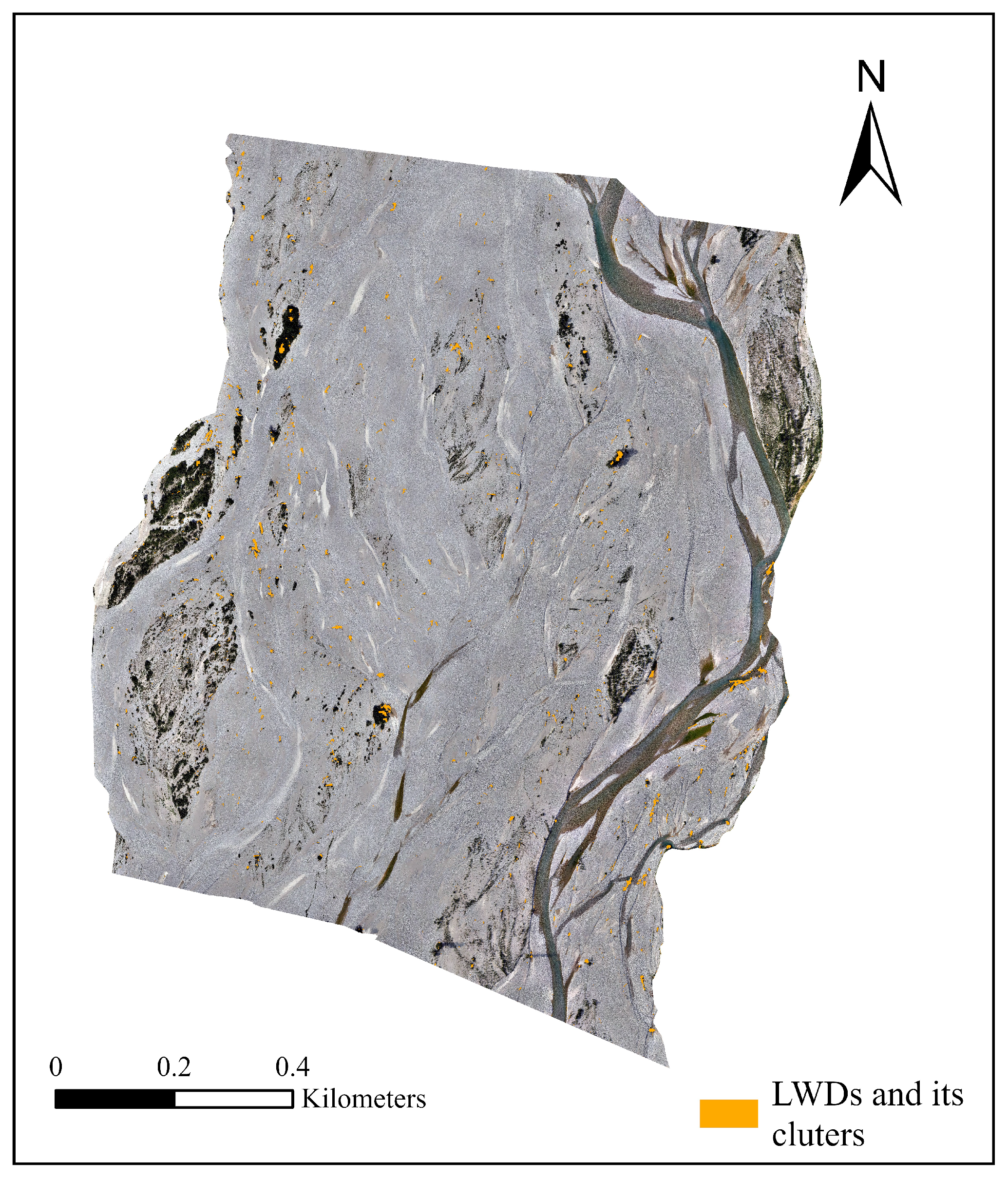
From a spatial perspective, the model successfully identified most of the LWD at both time points, and the predictions closely matched actual ground samples. Despite differences in environmental conditions between the image acquisition dates, the detection of major target areas remained consistent. The model demonstrated high detection accuracy and spatial consistency in larger areas and multiple temporal snapshots, indicating strong transferability and applicability in both spatial and temporal dimensions. The LWDs distribution map for the whole region can be found in Appendix A (Figure A1, Figure A2, Figure A3 and Figure A4), which includes the results for March and July.
In this study, Grad-CAM can be used to visualize the region of interest of the model when detecting LWD, thereby intuitively interpreting the model’s prediction results and verifying the reliability of the DL model in remote sensing object detection. As shown in Figure 11, Grad-CAM heatmap and predicted LWD probability map are analyzed to verify the interpretability of the model. The Grad-CAM heatmap shows that the model’s attention is mainly focused on the strip-like structures of the LWD, while the response to the background region is weak. Compared with the predicted LWD probability map, the model’s attention area is highly consistent with the high-probability region in space, indicating that the model relies on reasonable visual features when determining the location of the LWD, thereby enhancing the interpretability and credibility of the model’s prediction results.
Figure 11.
The interpretability of the model is visualized using Grad-CAM (partial display). The first column is the original RGB image. The second column is the Grad-CAM heatmap showing the visual regions that the model focuses on, brighter (yellow–red) regions indicate stronger activation responses. The third column is the predicted LWD probability map, with high-probability regions corresponding to the locations where the model determines the LWD to be.
4. Discussion
4.1. General Accuracy and Transferability
A model trained in one region can be effectively applied to a distant region, provided that the image and ground conditions remain similar [27]. This assumption forms the basis of the concept of model generalization, namely that the spatial and spectral patterns learned from the training region remain effective in new regions with similar environmental characteristics. In this study, the training and test regions have similar environmental conditions, supporting this assumption.
From an applied remote sensing perspective, such spatial transferability is essential to allow repeatable and scalable monitoring of LWD across river reaches without site-specific model retraining. When the model trained in a limited area was applied to a larger testing region, it achieved completeness and correctness values of 0.811 and 0.918 for March and 0.757 and 0.906 for July, respectively. The relatively lower completeness, particularly in July, may be attributed to several factors. First, increased solar radiation and higher solar zenith angles in July likely altered background reflectance conditions. Stronger illumination enhanced the brightness of exposed and dry gravel surfaces, increasing background heterogeneity, and reducing the spectral and structural contrast between LWD and surrounding substrates. In addition, seasonal drying of the wood surfaces may have modified their RGB reflectance characteristics, making them spectrally more similar to adjacent dry sediments. Second, hydrological differences in the Tagliamento River basin may have contributed to changes in surface moisture conditions. Spring snow melt typically produces higher discharge in March, while July is generally characterized by lower water level and drier climatic conditions. Although lower summer discharge exposes larger areas of gravel bars, the reduced surface moisture may decrease the natural color contrast between LWD and the surrounding substrate, increasing spectral confusion and thus missed detections. Third, phenological changes in the riparian vegetation during summer may have partially obscured LWD, particularly where LWD accumulated near vegetated bars or channel margins.
The accuracy metrics in this study were computed on a pixel basis rather than by counting individual detected objects, which is more appropriate for irregularly shaped or fragmented LWD. Comparable performance has been reported in previous research: Lopes Queiroz et al. [27] obtained completeness and correctness values of 0.769 and 0.870, Duan et al. [49] reported 0.757 and 0.925, and Jiang et al. [36] achieved approximately 0.678 and 0.990. Differences in reported accuracies across studies largely reflect variations in evaluation methods, image sources, data quality, and target characteristics. The results of this study indicate that the trained model demonstrates robust spatial generalization and strong transferability for LWDs mapping in braided river environments, supporting its potential use in operational monitoring.
Furthermore, the slight decrease in performance in the test region compared to the training region may be due to the increased background variability and morphological diversity of target objects when the model is transferred to a larger area. Similarly, if the model is applied to regions with significantly different substrates, water turbidity, or lighting conditions, its performance may decline. To mitigate this issue, the model can be fine-tuned using a small number of samples from the new region, thereby enhancing its robustness and maintaining accuracy under heterogeneous conditions.
4.2. Importance of Predictor Variables
RGB-UAV imagery, which lacks near-infrared and other multispectral bands, often provides limited spectral separability among surface classes when relying solely on spectral information. This limitation reduces the ability to effectively discriminate LWD from surrounding materials. The use of feature engineering helps mitigate this issue by introducing alternative, information-rich variables that enhance class distinction and improve model performance. In this study, both ML and DL models achieved markedly higher accuracy in the two-class classification compared to the more complex multi-class scheme, consistent with the findings of previous research [98,99].
Our results also highlight the critical role of texture features in LWD identification. LWD often exhibits unique linear structures and textural characteristics that cannot be captured by spectral values alone. In OBIA, image segmentation is based primarily on features such as texture. This explains the relatively high classification accuracy observed in the OBIA results, which is consistent with previous research [27,100,101]. PBIA, which classifies on the basis of individual pixel feature values, does not fully utilize the overall morphological and textural structure of LWD. This enables OBIA to detect LWD objects more effectively than PBIA. Furthermore, this also explains why OBIA achieves strong classification results even without the DSM feature combination.
The DSM performs well in the ML model, indicating that it can enhance ground object classification to some extent. However, it does not contribute comparably to the DL model. This discrepancy may be attributed to the stronger representation capacity of deep neural networks, which are able to automatically extract rich spatial and structural features from high-resolution RGB imagery, thereby reducing the reliance on explicit elevation inputs. From an architectural perspective, DeepLabv3+ employs the ASPP module, which extracts multi-scale contextual features through atrous convolutions with different rates. This design enables the network to capture fine-scale spatial patterns directly from RGB imagery, improve boundary delineation, and better preserve object edge information [102,103]. In high-resolution RGB imagery, morphological features such as texture gradients, object shape, and boundary discontinuities are strongly expressed. Similarly to previous studies [39,104], the marginal benefit of explicitly incorporating elevation data under such conditions may therefore be limited. In addition, resolution-related factors may further constrain the contribution of DSM. The DSM used in this study has a spatial resolution of approximately 10 cm, whereas the RGB orthophoto has a ground sampling distance of 2 cm. Although a resolution of 10 cm is theoretically sufficient to capture LWD morphological features at scales exceeding 1 m, the coarser resolution of the DSM may not provide additional effective information gain compared to the rich texture and edge information offered by the 2 cm RGB image. Moreover, potential noise and interpolation artifacts in DSM data may further reduce its effective contribution during deep feature extraction. From an applied perspective, this finding suggests that RGB-only imagery can be sufficient for reliable LWD detection when combined with appropriate spatial feature learning, reducing the dependence on additional elevation information.
Furthermore, analysis shows that RGB-based vegetation indices (such as NGBDI and NGRDI) contribute little to LWD classification in both PBIA and OBIA. This limited contribution may be due to the spectral similarity between LWD and some bare ground or unvegetated surfaces, which makes the vegetation indices less discriminative. Furthermore, this result highlights the importance of incorporating texture and geometric features in LWD classification. Relatively speaking, these features have stronger discriminative potential than traditional spectral indicators in high-resolution RGB images.
4.3. Advantages of DL Models
In this study, DL classification methods achieved the highest overall accuracy among all methods tested, demonstrating their superior ability to capture the complex spatial and spectral patterns associated with LWD distribution. This finding is consistent with previous deep learning studies [39,105], which report that convolutional architectures can effectively detect small irregular objects and that DL methods generally outperform traditional ML approaches.
From the perspective of model types, DeepLabv3+ consistently outperformed other models. In two-class classification tasks, DeepLabv3+ achieved significant improvements in F1-score and OA, demonstrating enhanced robustness and stability even in more challenging multi-class classification tasks. While PBIA and OBIA performed reasonably well in terms of OA, they struggled with misclassification control and were prone to the “salt and pepper effect”. PBIA, due to its pixel-level thresholding approach, is prone to misclassifying isolated or irregularly shaped objects, while OBIA relies heavily on segmentation quality. Although the U-Net model is capable of producing a reasonable boundary for LWD objects, the resulting edges tend to appear slightly fragmented and coarse, likely due to the model’s higher sensitivity to local texture variations. The superior performance of DeepLabv3+ is attributed to its encoder-decoder architecture, which incorporates dilated convolutions and an atrous spatial pyramid pooling (ASPP) module, which enables multi-scale feature extraction and enhances its ability to capture spatial contex [44,106,107]. This enables the model to better handle irregularly shaped and clustered LWD.
From a computational perspective, training DL models requires more powerful computing resources, including a sufficiently powerful GPU and runtime. Training can take tens or even hundreds of hours, while ML models can be completed in just a few hours on a standard CPU. In our experiments, inference over a 1 km river reach with 2 cm resolution imagery using DeepLabv3+ on an NVIDIA GPU required approximately several hours. This inference time is influenced by multiple factors, including image extent, spatial resolution (2 cm), GPU performance, and model complexity. Alternatively, where appropriate, using slightly lower spatial resolution (e.g., 5–10 cm) could substantially reduce processing time while potentially maintaining acceptable detection accuracy. Although DL requires more computing power and longer training times than traditional ML approaches, they provide more reliable and robust outputs. And once trained, its classification performance is excellent, capable of processing large numbers of pixels simultaneously, typically producing better results than traditional ML approaches [81]. Their advantages extend beyond improved accuracy to sensor utilization. High classification accuracy can be achieved even with only three visible bands, highlighting the potential of using only inexpensive visible-band cameras, eliminating the need for more expensive multispectral cameras.
In general, the classification results of the deep learning model closely reflect the actual spatial distribution of LWD observed in the field, including its morphology, density, and direction. This not only demonstrates quantitative reliability but also high spatial reliability, which is crucial for applications such as ecological monitoring and ecohydraulic modeling.
4.4. Limitation and Future Work
The reliability of the proposed method depends on the quality of the data which it is based. Various image artifacts, such as cloud shadows, illumination changes, and occlusion by vegetation or others, can interfere with the accurate identification of LWD. In particular, small objects may be missed due to image resolution limitations. Current sample data are based on manual interpretation, which may result in blurred boundaries and missing samples. Incorrect samples can also decrease training accuracy. Additionally, although labeling the entire region is not required, a large number of samples are still needed to ensure the effectiveness of model training. Therefore, while the model performs well overall, caution should be exercised in its application, especially in areas with complex environmental conditions or limited image quality.
Future work will focus on improving robustness by integrating multi-temporal imagery to mitigate the impact of transient noise such as shadows or seasonal changes. Integrating higher resolution data or combining optical imagery with complementary data sources may also enhance detection capabilities, especially for small or occluded objects. Future studies could also evaluate the model under extreme conditions, such as strong shadows, low-light environments, or partially submerged LWD, which may reduce the spectral and structural contrast between LWD and the surrounding background. In addition, expanding the training dataset to cover a wider range of scenarios and improving post-processing steps are also potential ways to reduce uncertainty and improve overall reliability.
5. Conclusions
This study developed and evaluated a robust deep learning framework for identifying and classifying large woody debris in braided river networks using centimeter-resolution RGB-UAV imagery. The performance of this framework was systematically compared with conventional pixel-based and object-based image analysis methods based on OA, F1-score, and IoU. The main conclusions are as follows.
1. The proposed deep learning framework exhibits strong generalizability. Using only RGB spectral information, the model effectively processes high-resolution UAV imagery and successfully transfers to different spatiotemporal areas with similar geomorphic characteristics, confirming its robustness and spatiotemporal adaptability in data-limited scenarios.
2. Superior spatial coherence of deep learning. Although OBIA slightly outperformed PBIA in accuracy, both traditional methods were affected by the “salt-and-pepper” effect, resulting in fragmented classifications. In contrast, the deep learning approach captured the spatial distribution patterns of large woody debris more continuously and accurately. Such spatial coherence is critical for applied studies that rely on realistic representations of LWDs distribution, including ecohydraulic and geomorphological analyzes.
3. Feature engineering in traditional methods shows clear benefits but inherent limitations. Although the combination of multiple features significantly improved the classification performance of both PBIA and OBIA, these methods remained prone to misclassification and noise in complex riparian environments. Texture features were more informative in OBIA, whereas vegetation indices such as NGBDI and NGRDI contributed minimally. Additionally, two-class classification consistently achieved higher accuracy and computational efficiency compared to multi-class classification.
The developed framework offers an efficient and automated tool for monitoring large woody debris and supporting the assessment of its eco-geomorphological functions in fluvial systems.
Author Contributions
Conceptualization, L.S. and C.C.; methodology, Q.H., E.B. and C.C.; software, Q.H.; validation, Q.H. and C.C.; formal analysis, Q.H. and E.B.; investigation, Q.H., L.S. and C.C.; resources, C.C.; data curation, Q.H., L.S. and U.M.d.C.; writing—original draft preparation, Q.H.; writing—review and editing, U.M.d.C., E.B. and C.C.; visualization, Q.H.; supervision, E.B. and C.C.; project administration, C.C.; funding acquisition, C.C. All authors have read and agreed to the published version of the manuscript.
Funding
This study was carried out within the project of “Eco–geomorphic carbon pumping from rivers to blue carbon Ecosystems (e–Capture)”—funded by the European Union—Next Generation EU within the PRIN 2022 program (D.D. 104 – 02/02/2022 Ministero dell’Università e della Ricerca; CUP E53D23004070006), by the European Union (Project Grant Agreement n.101185000–CONCERTO–HORIZON–CL5–2024–D1–01) and by the China Scholarship Council. Views and opinions expressed are however those of the author(s) only and do not necessarily reflect those of the European Union or the European Climate, Infrastructure and Environment Executive Agency (CINEA). Neither the European Union nor the granting authority can be held responsible for them.
Data Availability Statement
The training and evaluation samples used in this study are available at https://doi.org/10.5281/zenodo.17650507 (accessed on 30 December 2025) and python manipulation codes are available at https://github.com/qhan66/Detection-of-Large-woody-debris.git (accessed on 30 December 2025).
Acknowledgments
The authors sincerely thank all colleagues and collaborators who provided helpful comments and constructive feedback during the development of this study. The authors are also grateful to the anonymous reviewers for their valuable suggestions, which contributed to the improvement of this paper.
Conflicts of Interest
The authors declare that they have no known competing financial interests or personal relationships that could have appeared to influence the work reported in this paper.
Abbreviations
The following abbreviations are used in this manuscript:
| Acronym | Meaning |
| AI | artificial intelligence |
| CNN | Convolutional Neural Network |
| DL | Deep Learning |
| DSM | Digital Surface Model |
| EXG | Excess Green Index |
| FN | False Negatives |
| FP | False Positives |
| GLCM | Gray-level Co-occurrence Matrix |
| Grad-CAM | Gradient-weighted Class Activation Mapping |
| IoU | Intersection over Union |
| LWD | Large Woody Debris |
| ML | Machine Learning |
| NGBDI | Normalized Blue-green Index |
| NGRDI | Normalized Red-green Index |
| OA | Overall Accuracy |
| OBIA | Object-based Image Analyses |
| PBIA | Pixel-based Image Analyses |
| RF | Random Forest |
| RGRI | Red-Green Ratio Index |
| TP | True Positives |
| UAV | Unmanned Aerial Vehicle |
| VDVI | Visible-Band Difference Vegetation Index |
| VEGI | Vegetation Index |
Appendix A
Figure A1.
UAV-RGB images acquired in March 2024. This image served as the input data for the subsequent image classification process.
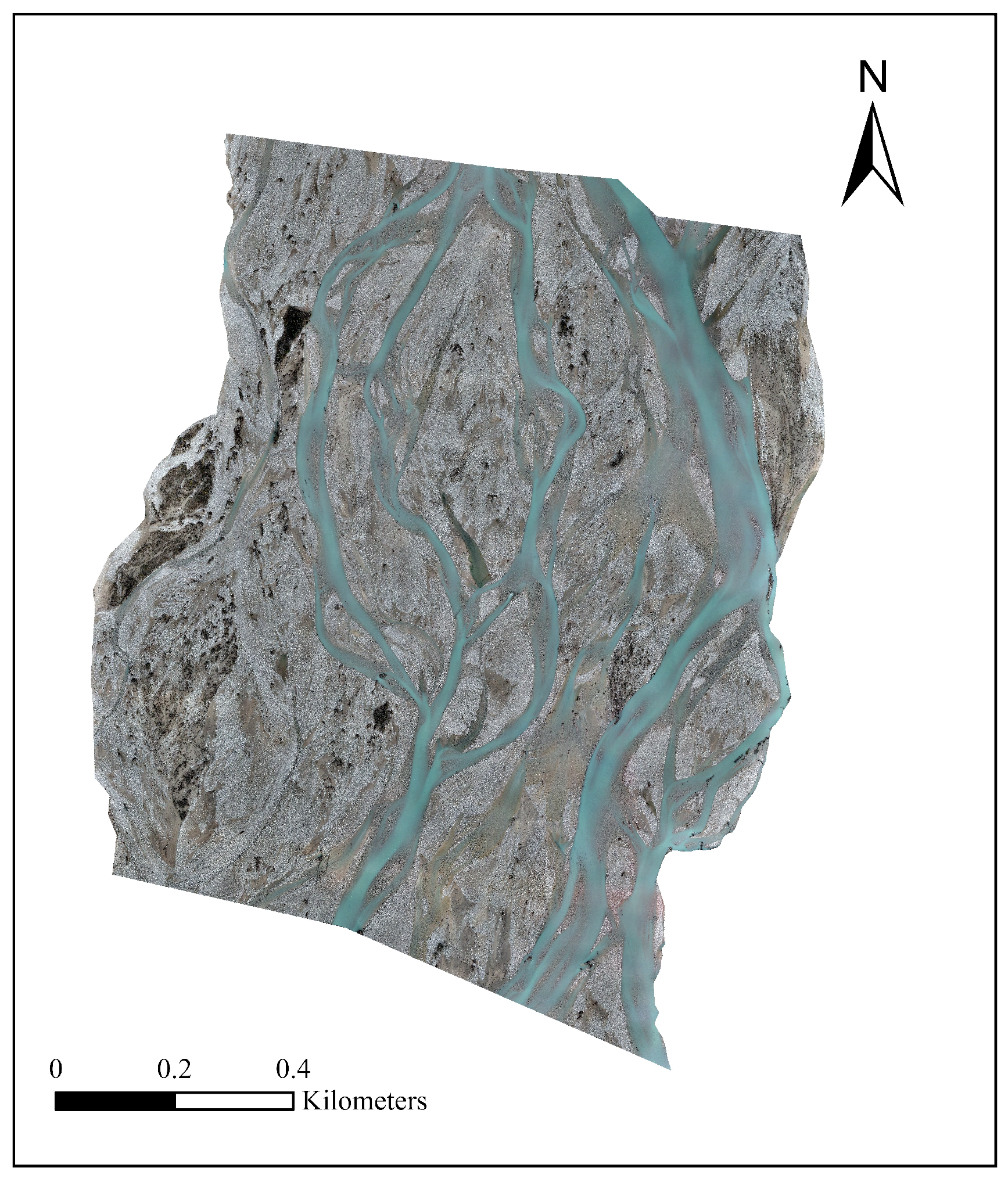
Figure A2.
Classification results for March 2024. The figure presents the output generated by the DeepLabv3+-based two-class classification model trained on UAV-RGB imagery, showing the spatial distribution of large woody debris.
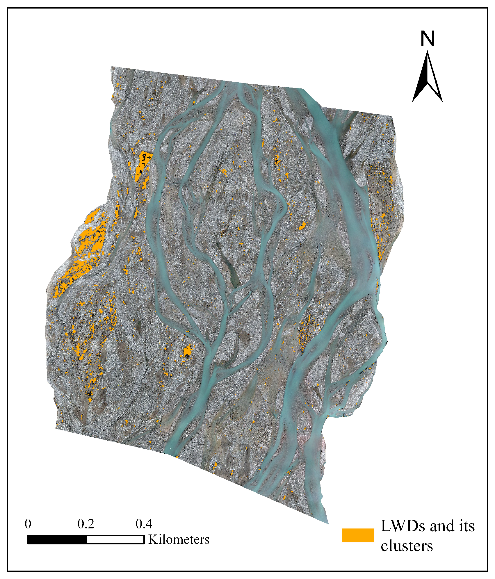
Figure A3.
UAV-RGB images acquired in July 2024. This image served as the input data for the subsequent image classification process.
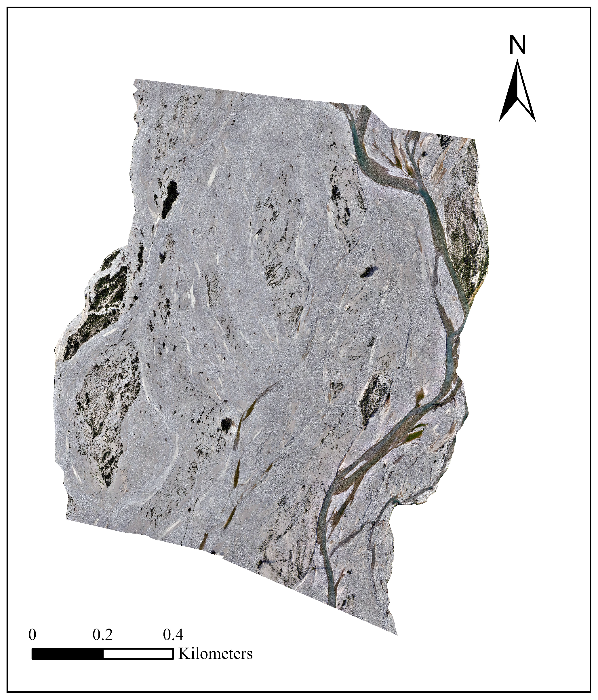
Figure A4.
Classification results for July 2024. The figure presents the output generated by the DeepLabv3+-based two-class classification model trained on UAV-RGB imagery, showing the spatial distribution of large woody debris.
References
- Gurnell, A.; England, J.; Burgess-Gamble, L. Trees and wood: Working with natural river processes. Water Environ. J. 2019, 33, 342–352. [Google Scholar] [CrossRef] [Scilit]
- Ravazzolo, D.; Spreitzer, G.; Tunnicliffe, J.; Friedrich, H. The effect of large wood accumulations with rootwads on local geomorphic changes. Water Resour. Res. 2022, 58, e2021WR031403. [Google Scholar] [CrossRef] [Scilit]
- Gurnell, A.M. Trees, wood and river morphodynamics: Results from 15 years research on the Tagliamento River, Italy. In River Science: Research and Management for the 21st Century; John Wiley & Sons, Ltd.: Hoboken, NJ, USA, 2016; pp. 132–155. [Google Scholar]
- Schalko, I.; Weitbrecht, V. Impact of large wood on river ecosystems. Water 2022, 14, 784. [Google Scholar] [CrossRef] [Scilit]
- Sanhueza, D.; Picco, L.; Paredes, A.; Iroumé, A. A Faster. Approach to Quantify Large Wood Using UAVs. Drones 2022, 6, 218. [Google Scholar] [CrossRef] [Scilit]
- Verdonschot, P.F.; Verdonschot, R.C. Ecological functions and management of large wood in fluvial systems. Curr. For. Rep. 2024, 10, 39–55. [Google Scholar]
- Wohl, E.; Kramer, N.; Ruiz-Villanueva, V.; Scott, D.N.; Comiti, F.; Gurnell, A.M.; Fausch, K.D. The natural wood regime in rivers. BioScience 2019, 69, 259–273. [Google Scholar] [CrossRef] [Scilit]
- Comiti, F.; Andreoli, A.; Lenzi, M.; Mao, L. Spatial density and characteristics of woody debris in five mountain rivers of the Dolomites (Italian Alps). Geomorphology 2006, 78, 44–63. [Google Scholar] [CrossRef] [Scilit]
- Lucía, A.; Comiti, F.; Borga, M.; Cavalli, M.; Marchi, L. Dynamics of large wood during a flash flood in two mountain catchments. Nat. Hazards Earth Syst. Sci. 2015, 15, 1741–1755. [Google Scholar] [CrossRef] [Scilit]
- Kramer, N.; Wohl, E.; Hess-Homeier, B.; Leisz, S. The pulse of driftwood export from a very large forested river basin over multiple time scales, Slave River, Canada. Water Resour. Res. 2017, 53, 1928–1947. [Google Scholar] [CrossRef] [Scilit]
- Sanhueza, D.; Picco, L.; Ruiz-Villanueva, V.; Iroumé, A.; Ulloa, H.; Barrientos, G. Quantification of fluvial wood using UAVs and structure from motion. Geomorphology 2019, 345, 106837. [Google Scholar] [CrossRef] [Scilit]
- Smikrud, K.M.; Prakash, A. Monitoring Large Woody Debris Dynamics in the Unuk River, Alaska Using Digital Aerial Photography. GIScience Remote Sens. 2006, 43, 142–154. [Google Scholar] [CrossRef] [Scilit]
- Marcus, W.A.; Legleiter, C.J.; Aspinall, R.J.; Boardman, J.W.; Crabtree, R.L. High spatial resolution hyperspectral mapping of in-stream habitats, depths, and woody debris in mountain streams. Geomorphology 2003, 55, 363–380. [Google Scholar] [CrossRef] [Scilit]
- Blanchard, S.D.; Jakubowski, M.K.; Kelly, M. Object-Based Image Analysis of Downed Logs in Disturbed Forested Landscapes Using Lidar. Remote Sens. 2011, 3, 2420–2439. [Google Scholar] [CrossRef] [Scilit]
- Abbe, T.B.; Montgomery, D.R. Large Woody Debris Jams, Channel Hydraulics and Habitat Formation in Large Rivers. Regul. Rivers Res. Manag. 1996, 12, 201–221. [Google Scholar] [CrossRef]
- Piégay, H. Dynamics of Wood in Large Rivers. Am. Fish. Soc. Symp. 2003, 37, 109–133. [Google Scholar]
- Comiti, F.; Pecorari, E.; Mao, L.; Picco, L.; Rigon, E.; Lenzi, M.A. New Methods for Determining Wood Storage and Mobility in Large Gravel-Bed Rivers—Deliverable D20bis; Technical Report; University of Padova: Padua, Italy, 2008. [Google Scholar]
- Ståhl, G.; Ringvall, A.; Fridman, J. Assessment of Coarse Woody Debris: A Methodological Overview. Ecol. Bull. 2001, 49, 57–70. [Google Scholar]
- Waser, L.T.; Küchler, M.; Jütte, K.; Stampfer, T. Evaluating the potential of WorldView-2 data to classify tree species and different levels of ash mortality. Remote Sens. 2014, 6, 4515–4545. [Google Scholar] [CrossRef] [Scilit]
- Ruiz-Villanueva, V.; Piégay, H.; Gurnell, A.M.; Marston, R.A.; Stoffel, M. Recent advances quantifying the large wood dynamics in river basins: New methods and remaining challenges. Rev. Geophys. 2016, 54, 611–652. [Google Scholar] [CrossRef] [Scilit]
- MacVicar, B.; Piégay, H. Implementation and validation of video monitoring for wood budgeting in a wandering piedmont river, the Ain River (France). Earth Surf. Process. Landf. 2012, 37, 1272–1289. [Google Scholar] [CrossRef] [Scilit]
- Ravazzolo, D.; Mao, L.; Picco, L.; Lenzi, M.A. Tracking log displacement during floods in the Tagliamento River using RFID and GPS tracker devices. Geomorphology 2015, 228, 226–233. [Google Scholar] [CrossRef] [Scilit]
- Iroumé, A.; Mao, L.; Ulloa, H.; Ruz, C.; Andreoli, A. Large wood volume and longitudinal distribution in channel segments draining catchments with different land use. Open J. Mod. Hydrol. 2014, 4, 57–66. [Google Scholar]
- Marcus, W.A.; Marston, R.A.; Colvard, C.R.; Gray, R.D. Mapping the spatial and temporal distributions of large woody debris in rivers of the Greater Yellowstone Ecosystem, U.S.A. Geomorphology 2002, 44, 323–335. [Google Scholar] [CrossRef] [Scilit]
- MacVicar, B.J.; Piégay, H.; Henderson, A.; Comiti, F.; Oberlin, C.; Pecorari, E. Quantifying the temporal dynamics of wood in large rivers: Field trials of wood surveying, dating, tracking, and monitoring techniques. Earth Surf. Process. Landf. 2009, 34, 2031–2046. [Google Scholar]
- Richardson, J.J.; Moskal, L.M. An integrated approach for monitoring contemporary and recruitable large woody debris. Remote Sens. 2016, 8, 778. [Google Scholar] [CrossRef] [Scilit]
- Lopes Queiroz, G.; McDermid, G.J.; Castilla, G.; Linke, J.; Rahman, M.M. Mapping coarse woody debris with random forest classification of centimetric aerial imagery. Forests 2019, 10, 471. [Google Scholar] [CrossRef] [Scilit]
- Wright, A.; Marcus, W.A.; Aspinall, R.J. Evaluation of Multispectral, Fine Scale Digital Imagery. Geomorphology 2000, 33, 107–120. [Google Scholar] [CrossRef] [Scilit]
- Truksa, T.; Bowman, J.; Goode, J. Can drones measure LWD?: High resolution aerial imagery and structure from motion as a method for quantifying instream wood. Geol. Soc. Am. Abstr. 2017, 49, 308662. [Google Scholar]
- Zhang, Z.; Huang, L.; Wang, Q.; Jiang, L.; Qi, Y.; Wang, S.; Shen, T.; Tang, B.H.; Gu, Y. UAV Hyperspectral Remote Sensing Image Classification: A Systematic Review. IEEE J. Sel. Top. Appl. Earth Obs. Remote Sens. 2025, 18, 3099–3124. [Google Scholar] [CrossRef] [Scilit]
- Hortobágyi, B.; Petit, S.; Marteau, B.; Melun, G.; Piégay, H. A high-resolution inter-annual framework for exploring hydrological drivers of large wood dynamics. River Res. Appl. 2024, 40, 958–975. [Google Scholar] [CrossRef] [Scilit]
- Liang, M.C.; Tfwala, S.S.; Chen, S.C. The evaluation of color spaces for large woody debris detection in rivers using XGBoost algorithm. Remote Sens. 2022, 14, 998. [Google Scholar] [CrossRef] [Scilit]
- Dos Santos, R.C.; Shin, S.Y.; Manish, R.; Zhou, T.; Fei, S.; Habib, A. General Approach for Forest Woody Debris Detection in Multi-Platform LiDAR Data. Remote Sens. 2025, 17, 651. [Google Scholar] [CrossRef] [Scilit]
- Windrim, L.; Bryson, M.; McLean, M.; Randle, J.; Stone, C. Automated mapping of woody debris over harvested forest plantations using UAVs, high-resolution imagery, and machine learning. Remote Sens. 2019, 11, 733. [Google Scholar] [CrossRef] [Scilit]
- Nakata, Y.; Hayamizu, M.; Ishiyama, N. Spatiotemporal Monitoring of Large Woody Debris Mobility and Distribution Using Unmanned Aerial Vehicles Along the Oshirarika River, Northern Japan. Drones 2025, 9, 655. [Google Scholar] [CrossRef] [Scilit]
- Jiang, S.; Yao, W.; Heurich, M. Dead wood detection based on semantic segmentation of VHR aerial CIR imagery using optimized FCN-Densenet. Int. Arch. Photogramm. Remote Sens. Spat. Inf. Sci. 2019, 42, 127–133. [Google Scholar] [CrossRef] [Scilit]
- Blackburn, R.C.; Buscaglia, R.; Sánchez Meador, A.J.; Moore, M.M.; Sankey, T.; Sesnie, S.E. Eigenfeature-enhanced deep learning: Advancing tree species classification in mixed conifer forests with lidar. Remote Sens. Ecol. Conserv. 2025, 11, 670–685. [Google Scholar]
- Osco, L.P.; Junior, J.M.; Ramos, A.P.M.; Jorge, L.A.C.; Fatholahi, S.N.; Silva, J.A.; Matsubara, E.T.; Pistori, H.; Gonçalves, W.N.; Li, J. A Review on Deep Learning in UAV Remote Sensing. arXiv 2021, arXiv:2101.10861. [Google Scholar] [CrossRef] [Scilit]
- Zheng, J.Y.; Hao, Y.Y.; Wang, Y.C.; Zhou, S.Q.; Wu, W.B.; Yuan, Q.; Zhao, B. Coastal wetland vegetation classification using pixel-based, object-based and deep learning methods based on RGB-UAV. Land 2022, 11, 2039. [Google Scholar] [CrossRef] [Scilit]
- Emek Soylu, B.; Guzel, M.S.; Bostanci, G.E.; Ekinci, F.; Asuroglu, T.; Acici, K. Deep-learning-based approaches for semantic segmentation of natural scene images: A review. Electronics 2023, 12, 2730. [Google Scholar] [CrossRef] [Scilit]
- Likó, S.B.; Holb, I.J.; Oláh, V.; Burai, P.; Szabó, S. Deep learning-based training data augmentation combined with post-classification improves the classification accuracy for dominant and scattered invasive forest tree species. Remote Sens. Ecol. Conserv. 2024, 10, 203–219. [Google Scholar] [CrossRef] [Scilit]
- Zhao, Q.; Cao, J.; Ge, J.; Zhu, Q.; Chen, X.; Liu, W. Multi-UNet: An effective Multi-U convolutional networks for semantic segmentation. Knowl.-Based Syst. 2025, 309, 112854. [Google Scholar]
- Bhatnagar, S.; Gill, L.; Ghosh, B. Drone image segmentation using machine and deep learning for mapping raised bog vegetation communities. Remote Sens. 2020, 12, 2602. [Google Scholar]
- Gonzalez-Perez, A.; Abd-Elrahman, A.; Wilkinson, B.; Johnson, D.J.; Carthy, R.R. Deep and machine learning image classification of coastal wetlands using unpiloted aircraft system multispectral images and lidar datasets. Remote Sens. 2022, 14, 3937. [Google Scholar] [CrossRef] [Scilit]
- Martínez Prentice, R.; Villoslada Peciña, M.; Ward, R.D.; Bergamo, T.F.; Joyce, C.B.; Sepp, K. Machine Learning Classification and Accuracy Assessment from High-Resolution Images of Coastal Wetlands. Remote Sens. 2021, 13, 3669. [Google Scholar] [CrossRef] [Scilit]
- Chaturvedi, P.; Johenneken, M.; Drak, A.; Houben, S.; Asteroth, A. Object-Based Tree Stump Detection Fusing RGB and Multispectral Data. In 2023 International Conference on Software, Telecommunications and Computer Networks (SoftCOM); IEEE: New York, NY, USA, 2023; pp. 1–6. [Google Scholar]
- Zielewska-Büttner, K.; Adler, P.; Kolbe, S.; Beck, R.; Ganter, L.M.; Koch, B.; Braunisch, V. Detection of standing deadwood from aerial imagery products: Two methods for addressing the bare ground misclassification issue. Forests 2020, 11, 801. [Google Scholar] [CrossRef] [Scilit]
- Blaschke, T. Object based image analysis for remote sensing. ISPRS J. Photogramm. Remote Sens. 2010, 65, 2–16. [Google Scholar]
- Duan, F.; Wan, Y.; Deng, L. A novel approach for coarse-to-fine windthrown tree extraction based on unmanned aerial vehicle images. Remote Sens. 2017, 9, 306. [Google Scholar]
- Francis, R.A.; Tibaldeschi, P.; McDougall, L. Fluvially-deposited large wood and riparian plant diversity. Wetl. Ecol. Manag. 2008, 16, 371–382. [Google Scholar] [CrossRef] [Scilit]
- Petts, G.E.; Gurnell, A.M.; Gerrard, A.J.; Hannah, D.M.; Hansford, B.; Morrissey, I.; Edwards, P.J.; Kollmann, J.; Ward, J.V.; Tockner, K.; et al. Longitudinal variations in exposed riverine sediments: A context for the ecology of the Fiume Tagliamento, Italy. Aquat. Conserv. Mar. Freshw. Ecosyst. 2000, 10, 249–266. [Google Scholar] [CrossRef] [Scilit]
- Tockner, K.; Ward, J.V.; Arscott, D.B.; Edwards, P.J.; Kollmann, J.; Gurnell, A.M.; Petts, G.E.; Maiolini, B. The Tagliamento River: A model ecosystem of European importance. Aquat. Sci. 2003, 65, 239–253. [Google Scholar] [CrossRef] [Scilit]
- Ward, J.V.; Tockner, K.; Edwards, P.J.; Kollmann, J.; Bretschko, G.; Gurnell, A.M.; Petts, G.E.; Rossaro, B. A reference system for the Alps: The ‘Fiume Tagliamento’. Regul. Rivers: Res. Manag. 1999, 15, 63–75. [Google Scholar] [CrossRef] [Scilit]
- Gurnell, A.M.; Petts, G.E.; Hannah, D.M.; Smith, B.P.G.; Edwards, P.J.; Kollmann, J.; Ward, J.V.; Tockner, K. Island formation along the gravel-bed Fiume Tagliamento, Italy. Earth Surf. Process. Landf. 2001, 26, 31–62. [Google Scholar] [CrossRef] [Scilit]
- Mao, L.; Ravazzolo, D.; Picco, L.; Rigon, E.; Lenzi, M.A. Types and volume of in-channel wood in three Italian gravel bed rivers suffering from different degrees of human disturbances. In Proceedings of the International Conference on Integrative Sciences and Sustainable Development of Rivers, Lyon, France, 26–28 June 2012; pp. 26–28. [Google Scholar]
- Lastilla, L.; Ravanelli, R.; Crespi, M. First test of Agisoft Metashape satellite image processing for DSM generation: A case study in Trento with Pléiades imagery. In IGARSS 2020–2020 IEEE International Geoscience and Remote Sensing Symposium; IEEE: New York, NY, USA, 2020; pp. 897–900. [Google Scholar]
- Agisoft LLC. Agisoft Metashape User Manual: Professional Edition. Version 2.1. Available online: https://www.agisoft.com/downloads/user-manuals/ (accessed on 1 July 2024).
- Nargesian, F.; Samulowitz, H.; Khurana, U.; Khalil, E.B.; Turaga, D.S. Learning Feature Engineering for Classification. In Proceedings of the International Joint Conference on Artificial Intelligence (IJCAI-17), Melbourne, Australia, 19–25 August 2017; pp. 2529–2535. [Google Scholar]
- Zhong, Z.; Li, J.; Luo, Z.; Chapman, M. Spectral–Spatial Residual Network for Hyperspectral Image Classification: A 3-D Deep Learning Framework. IEEE Trans. Geosci. Remote Sens. 2018, 56, 847–858. [Google Scholar] [CrossRef] [Scilit]
- Zheng, A.; Casari, A. Feature Engineering for Machine Learning: Principles and Techniques for Data Scientists; O’Reilly Media: Sebastopol, CA, USA, 2018. [Google Scholar]
- Jia, X.; Kuo, B.-C.; Crawford, M.M. Feature Mining for Hyperspectral Image Classification. Proc. IEEE 2013, 101, 676–697. [Google Scholar] [CrossRef] [Scilit]
- Torres-Sánchez, J.; Peña, J.M.; de Castro, A.I.; López-Granados, F. Multi-Temporal Mapping of the Vegetation Fraction in Early-Season Wheat Fields Using Images from UAV. Comput. Electron. Agric. 2014, 103, 104–113. [Google Scholar] [CrossRef] [Scilit]
- Du, M.; Noguchi, N. Monitoring of Wheat Growth Status and Mapping of Wheat Yield’s Within-Field Spatial Variations Using Color Images Acquired from UAV-Camera System. Remote Sens. 2017, 9, 289. [Google Scholar] [CrossRef] [Scilit]
- Wang, X.; Wang, M.; Wang, S.; Wu, Y. Extraction of vegetation information from visible unmanned aerial vehicle images. Trans. Chin. Soc. Agric. Eng. 2015, 31, 152–159. [Google Scholar]
- Lee, M.K.; Golzarian, M.R.; Kim, I.A. A new color index for vegetation segmentation and classification. Precis. Agric. 2021, 22, 179–204. [Google Scholar] [CrossRef] [Scilit]
- Woebbecke, D.M.; Meyer, G.E.; VanBargen, K.; Mortensen, D.A. Color Indices for Weed Identification Under Various Soil, Residue, and Lighting Conditions. Trans. ASAE 1995, 38, 259–269. [Google Scholar] [CrossRef] [Scilit]
- Marchant, J.A.; Onyango, C.M. Shadow-Invariant Classification for Scenes Illuminated by Daylight. J. Opt. Soc. Am. A 2000, 17, 1952. [Google Scholar] [CrossRef] [Scilit] [PubMed]
- Hague, T.; Tillett, N.D.; Wheeler, H.J.P.A. Automated crop and weed monitoring in widely spaced cereals. Precis. Agric. 2006, 7, 21–32. [Google Scholar] [CrossRef] [Scilit]
- Haralick, R.M.; Shanmugam, K. Textural features for image classification. IEEE Trans. Syst. Man Cybern. 1973, 6, 610–621. [Google Scholar] [CrossRef] [Scilit]
- Reed, B.; Brown, J.; Vanderzee, D.; Loveland, T.; Merchant, J.; Ohlen, D. Measuring Phenological Variability from Satellite Imagery. J. Veg. Sci. 1994, 5, 703–714. [Google Scholar] [CrossRef] [Scilit]
- Christophe, E.; Inglada, J.; Giros, A. Orfeo toolbox: A complete solution for mapping from high resolution satellite images. Int. Arch. Photogramm. Remote Sens. Spat. Inf. Sci. 2008, 37, 1263–1268. [Google Scholar]
- Szantoi, Z.; Malone, S.; Escobedo, F.; Misas, O.; Smith, S.; Dewitt, B. A tool for rapid post-hurricane urban tree debris estimates using high resolution aerial imagery. Int. J. Appl. Earth Obs. Geoinf. 2012, 18, 548–556. [Google Scholar] [CrossRef] [Scilit]
- Belcore, E.; Piras, M.; Pezzoli, A. Land Cover Classification from Very High-Resolution UAS Data for Flood Risk Mapping. Sensors 2022, 22, 5622. [Google Scholar] [CrossRef] [Scilit]
- Baatz, M. Multiresolution segmentation: An optimization approach for high quality multi-scale image segmentation. In Angewandte Geographische Informationsverarbeitung XII; Wichmann: Karlsruhe, Germany, 2000; pp. 12–23. [Google Scholar]
- Hossain, M.D.; Chen, D. Segmentation for Object-Based Image Analysis (OBIA): A Review of Algorithms and Challenges from Remote Sensing Perspective. ISPRS J. Photogramm. Remote Sens. 2019, 150, 115–134. [Google Scholar] [CrossRef] [Scilit]
- Kingma, D.P.; Ba, J. Adam: A Method for Stochastic Optimization. arXiv 2014, arXiv:1412.6980. [Google Scholar]
- Kattenborn, T.; Leitloff, J.; Schiefer, F.; Hinz, S. Review on Convolutional Neural Networks (CNN) in vegetation remote sensing. ISPRS J. Photogramm. Remote Sens. 2021, 173, 24–49. [Google Scholar] [CrossRef] [Scilit]
- Vakalopoulou, M.; Christodoulidis, S.; Burgos, N.; Colliot, O.; Lepetit, V. Deep learning: Basics and convolutional neural networks (CNNs). In Machine Learning for Brain Disorders; Springer: Berlin/Heidelberg, Germany, 2023; pp. 77–115. [Google Scholar]
- Badrinarayanan, V.; Kendall, A.; Cipolla, R. SegNet: A Deep Convolutional Encoder-Decoder Architecture for Image Segmentation. IEEE Trans. Pattern Anal. Mach. Intell. 2017, 39, 2481–2495. [Google Scholar] [CrossRef] [Scilit]
- Eigen, D.; Fergus, R. Predicting Depth, Surface Normals and Semantic Labels with a Common Multi-Scale Convolutional Architecture. In Proceedings of the IEEE International Conference on Computer Vision (ICCV), Santiago, Chile, 7–13 December 2015; pp. 2650–2658. [Google Scholar]
- Kislov, D.E.; Korznikov, K.A.; Altman, J.; Vozmishcheva, A.S.; Krestov, P.V. Extending deep learning approaches for forest disturbance segmentation on very high-resolution satellite images. Remote Sens. Ecol. Conserv. 2021, 7, 355–368. [Google Scholar] [CrossRef] [Scilit]
- Michez, A.; Piégay, H.; Lisein, J.; Claessens, H.; Lejeune, P. Classification of riparian forest species and health condition using multi-temporal and hyperspatial imagery from unmanned aerial system. Environ. Monit. Assess. 2016, 188, 146. [Google Scholar] [CrossRef] [Scilit] [PubMed]
- Aldous, A.; Schill, S.; Raber, G.; Paiz, M.C.; Mambela, E.; Stévart, T. Mapping complex coastal wetland mosaics in Gabon for informed ecosystem management: Use of object-based classification. Remote Sens. Ecol. Conserv. 2021, 7, 64–79. [Google Scholar] [CrossRef] [Scilit]
- Esri. Train Random Trees Classifier (Image Analyst). Available online: https://doc.arcgis.com/en/allsource/1.3/analysis/geoprocessing-tools/image-analyst/train-random-trees-classifier.htm (accessed on 23 October 2025).
- Menze, B.H.; Kelm, B.M.; Masuch, R.; Himmelreich, U.; Bachert, P.; Petrich, W.; Hamprecht, F.A. A comparison of random forest and its Gini importance with standard chemometric methods for the feature selection and classification of spectral data. BMC Bioinform. 2009, 10, 213. [Google Scholar] [CrossRef] [Scilit]
- Breiman, L.; Friedman, J.; Olshen, R.A.; Stone, C.J. Classification and Regression Trees; Routledge: Abingdon, UK, 2017. [Google Scholar]
- Tan, K.; Zhang, Y.; Wang, X.; Chen, Y. Object-Based Change Detection Using Multiple Classifiers and Multi-Scale Uncertainty Analysis. Remote Sens. 2019, 11, 359. [Google Scholar] [CrossRef] [Scilit]
- Galia, T.; Poledniková, Z.; Kapustová, V.; Ruiz-Villanueva, V.; Škarpich, V. Interannual spatial distribution and dynamics of large wood in a meandering river. J. Hydrol. 2025, 659, 133302. [Google Scholar] [CrossRef] [Scilit]
- Dice, L.R. Measures of the Amount of Ecologic Association Between Species. Ecology 1945, 26, 297–302. [Google Scholar] [CrossRef] [Scilit]
- Huang, L.; Jiang, B.; Lv, S.; Liu, Y.; Fu, Y. Deep-learning-based semantic segmentation of remote sensing images: A survey. IEEE J. Sel. Top. Appl. Earth Obs. Remote Sens. 2023, 17, 8370–8396. [Google Scholar] [CrossRef] [Scilit]
- Latella, M.; Sola, F.; Camporeale, C. A Density-Based Algorithm for the Detection of Individual Trees from LiDAR Data. Remote Sens. 2021, 13, 322. [Google Scholar] [CrossRef] [Scilit]
- Goutte, C.; Gaussier, E. A Probabilistic Interpretation of Precision, Recall and F-Score, with Implication for Evaluation. In Advances in Information Retrieval; Springer: Berlin/Heidelberg, Germany, 2005; pp. 345–359. [Google Scholar]
- Rahman, M.A.; Wang, Y. Optimizing Intersection-Over-Union in Deep Neural Networks for Image Segmentation. In Advances in Visual Computing. ISVC 2016; Lecture Notes in Computer Science; Springer: Berlin/Heidelberg, Germany, 2016; p. 10072. [Google Scholar] [CrossRef] [Scilit]
- Selvaraju, R.R.; Cogswell, M.; Das, A.; Vedantam, R.; Parikh, D.; Batra, D. Grad-CAM: Visual Explanations from Deep Networks via Gradient-Based Localization. In Proceedings of the 2017 IEEE International Conference on Computer Vision (ICCV), Venice, Italy, 22–29 October 2017; pp. 618–626. [Google Scholar] [CrossRef] [Scilit]
- Ebrahimi, S.; Kumar, S. What Helps to Detect What? Explainable AI and Multisensor Fusion for Semantic Segmentation of Simultaneous Crop and Land Cover Land Use Delineation. IEEE J. Sel. Top. Appl. Earth Obs. Remote Sens. 2025, 18, 5423–5444. [Google Scholar] [CrossRef] [Scilit]
- Ahad, T.; Kibria, H.B.; Mehemud, M.Y. MultiClass Classification of Chest Diseases using CXR Images with DenseNet201+CNN and Grad CAM Visualization. In Proceedings of the 2024 IEEE International Conference on Power, Electrical, Electronics and Industrial Applications (PEEIACON), Rajshahi, Bangladesh, 12–13 September 2024; pp. 368–372. [Google Scholar] [CrossRef] [Scilit]
- Srivastava, N.; Hinton, G.; Krizhevsky, A.; Sutskever, I.; Salakhutdinov, R. Dropout: A simple way to prevent neural networks from overfitting. J. Mach. Learn. Res. 2014, 15, 1929–1958. [Google Scholar]
- Luo, C.; Li, X.; Yin, J.; He, J.; Li, D.; Zhou, J. How does the data set and the number of categories affect CNN-based image classification performance? J. Softw. 2019, 14, 168–181. [Google Scholar] [CrossRef] [Scilit]
- Van Thinh, T.; Duong, P.C.; Nasahara, K.N.; Tadono, T. How does land use/land cover map’s accuracy depend on number of classification classes? SOLA 2019, 15, 28–31. [Google Scholar] [CrossRef] [Scilit]
- Zhou, R.; Yang, C.; Li, E.; Cai, X.; Yang, J.; Xia, Y. Object-based wetland vegetation classification using multi-feature selection of unoccupied aerial vehicle RGB imagery. Remote Sens. 2021, 13, 4910. [Google Scholar] [CrossRef] [Scilit]
- Feng, S.; Li, W.; Xu, J.; Liang, T.; Ma, X.; Wang, W.; Yu, H. Land use/land cover mapping based on GEE for the monitoring of changes in ecosystem types in the upper Yellow River basin over the Tibetan Plateau. Remote Sens. 2022, 14, 5361. [Google Scholar] [CrossRef] [Scilit]
- Du, S.; Du, S.; Liu, B.; Zhang, X. Incorporating DeepLabv3+ and object-based image analysis for semantic segmentation of very high resolution remote sensing images. Int. J. Digit. Earth 2021, 14, 357–378. [Google Scholar] [CrossRef] [Scilit]
- Wang, Y.; Yang, L.; Liu, X.; Yan, P. An improved semantic segmentation algorithm for high-resolution remote sensing images based on DeepLabv3+. Sci. Rep. 2024, 14, 9716. [Google Scholar] [CrossRef] [Scilit]
- Paredes, A.; Martini, L.; Sanchéz, K.; Iroumé, A.; Picco, L. Automatic detection of in-channel wood using UAV-based deep learning: A scalable approach for river monitoring. Geomorphology 2026, 500, 110223. [Google Scholar] [CrossRef] [Scilit]
- Fang, W.; Wang, C.; Chen, X.; Wan, W.; Li, H.; Zhu, S.; Fang, Y.; Liu, B.; Hong, Y. Recognizing global reservoirs from Landsat 8 images: A deep learning approach. IEEE J. Sel. Top. Appl. Earth Obs. Remote Sens. 2019, 12, 3168–3177. [Google Scholar] [CrossRef] [Scilit]
- Chen, L.-C.; Zhu, Y.; Papandreou, G.; Schroff, F.; Adam, H. Encoder-Decoder with Atrous Separable Convolution for Semantic Image Segmentation. In Computer Vision—ECCV 2018; Springer: Berlin/Heidelberg, Germany, 2018; pp. 801–818. [Google Scholar] [CrossRef] [Scilit]
- Wei, D.; Xie, H.; Li, P.; Xu, Y. A Learning Framework with Multispectral Band-Differentiated Encoding for Remote Sensing Water Body Detection. IEEE J. Sel. Top. Appl. Earth Obs. Remote Sens. 2024, 17, 6278–6289. [Google Scholar] [CrossRef] [Scilit]
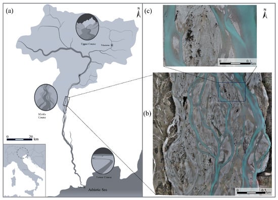
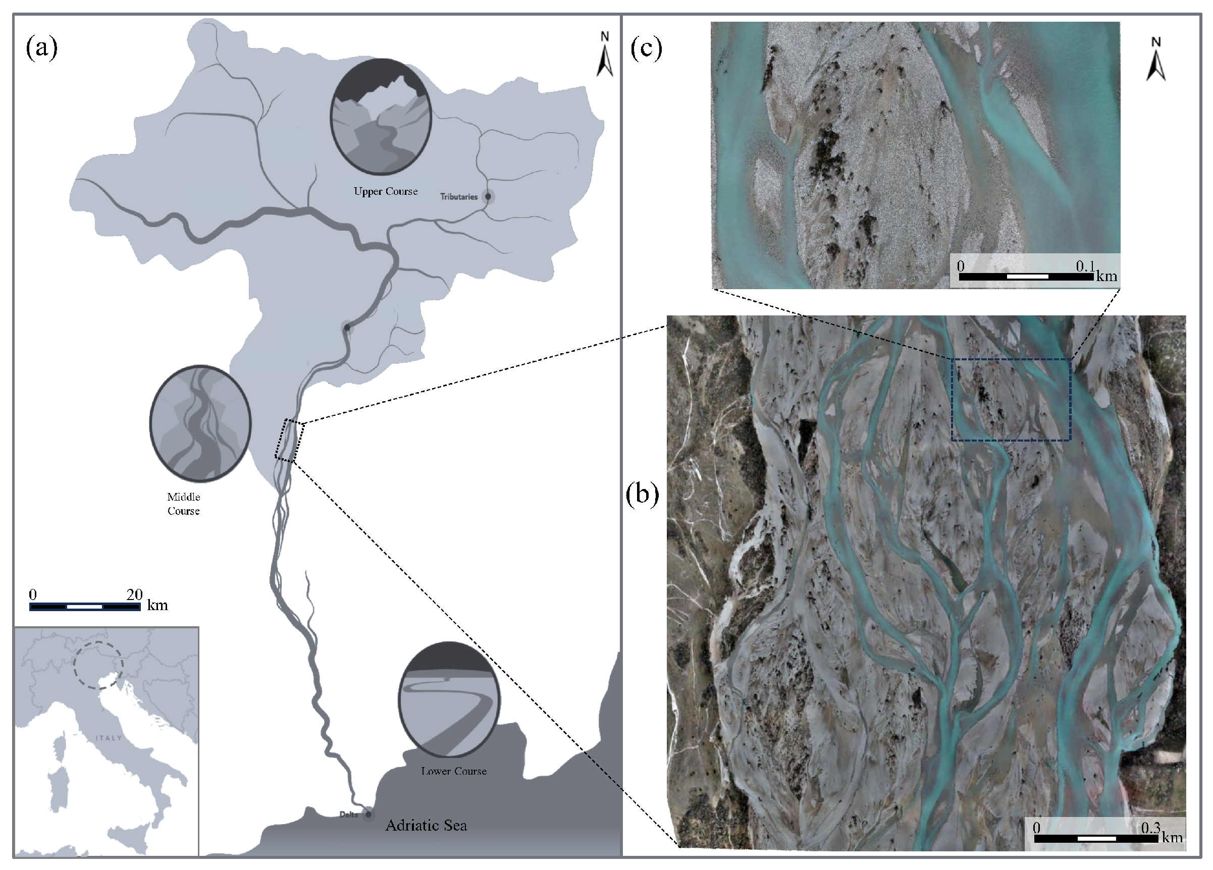
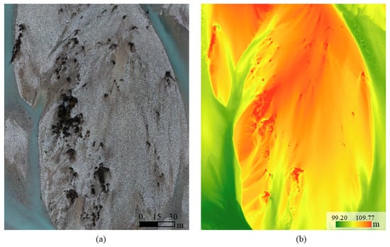
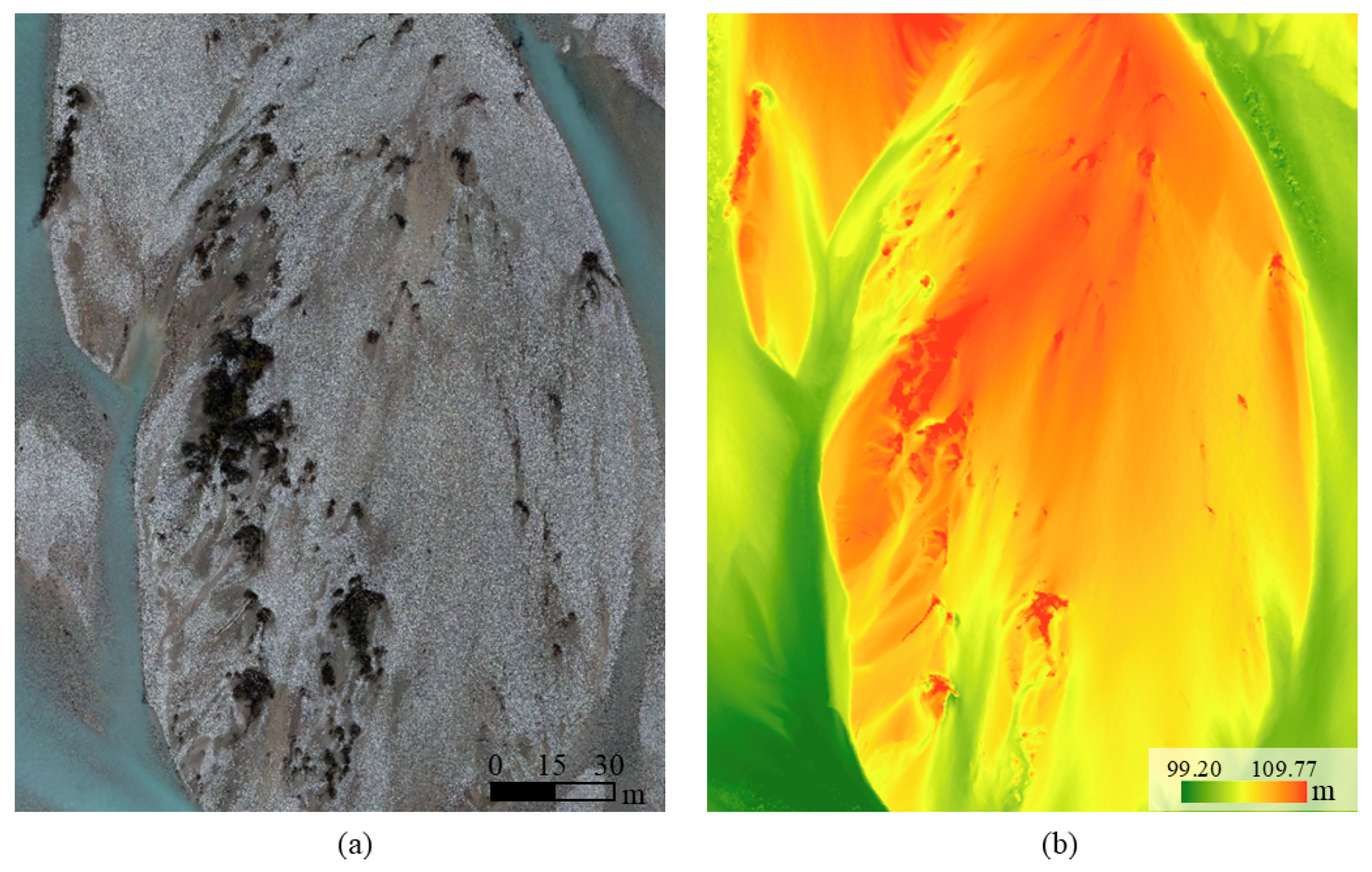
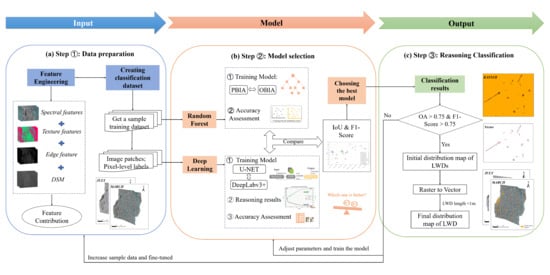
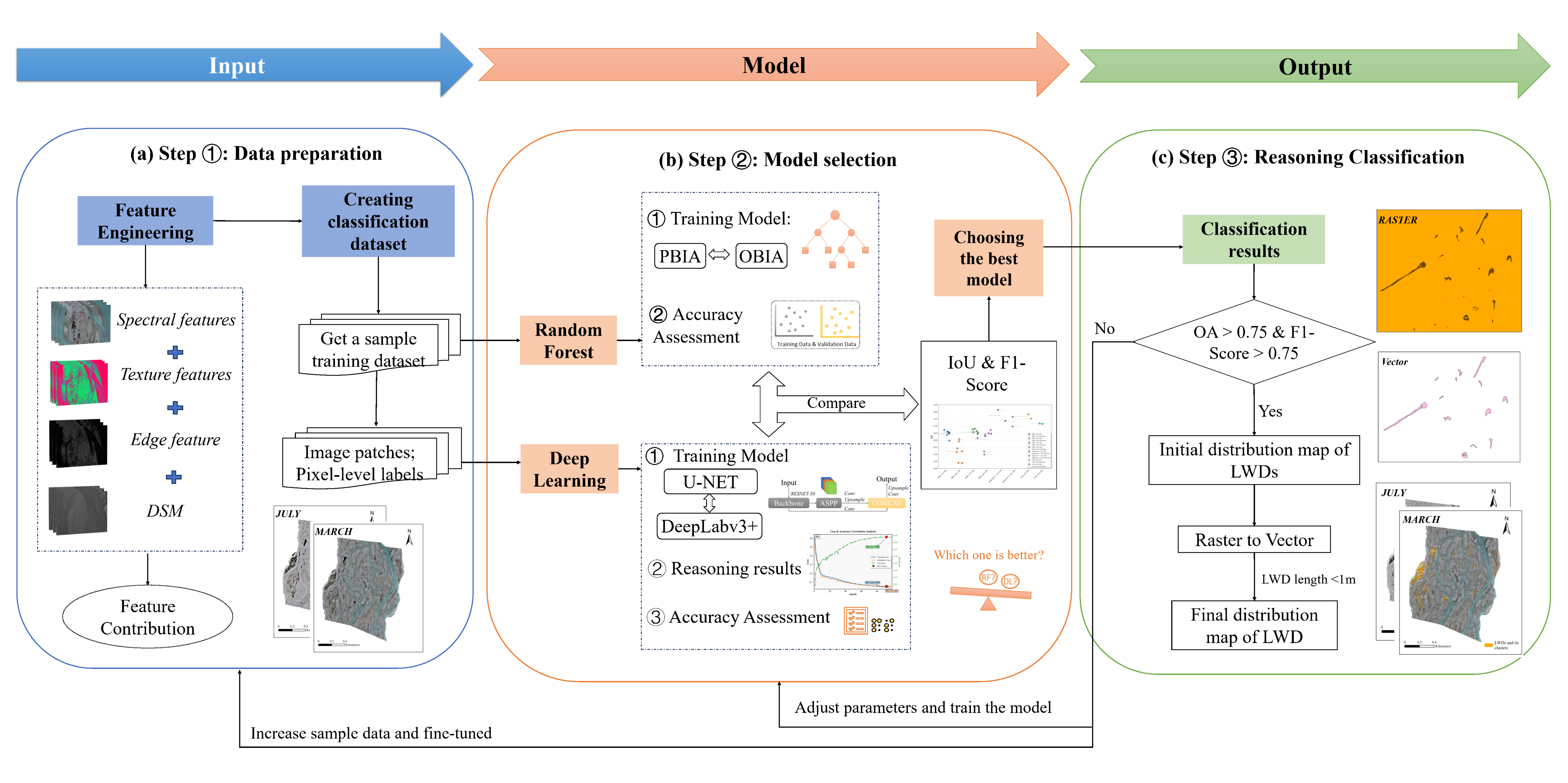
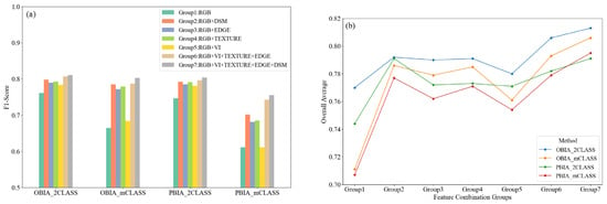
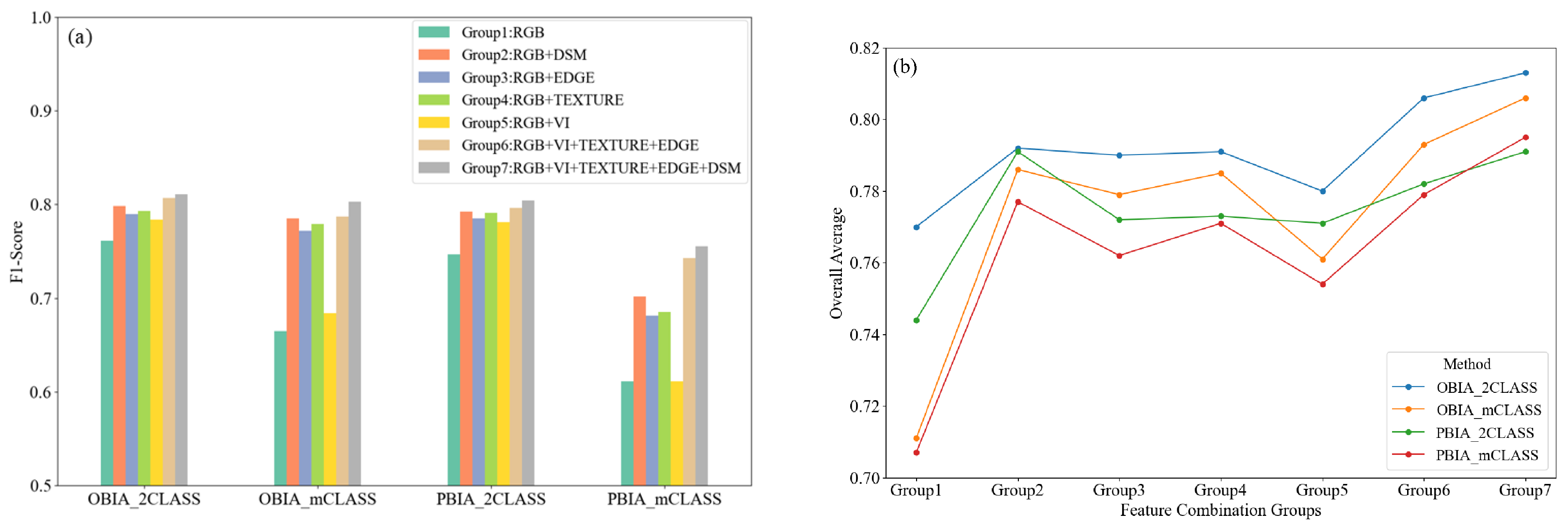
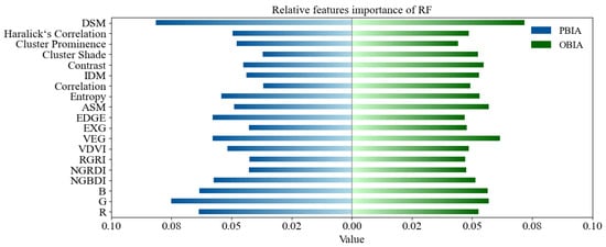
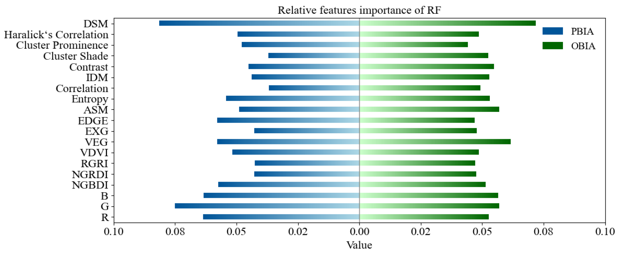
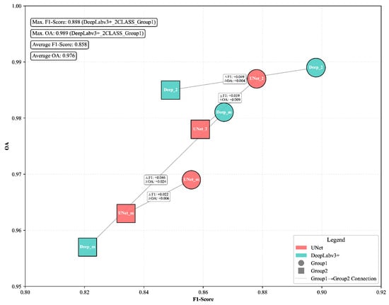
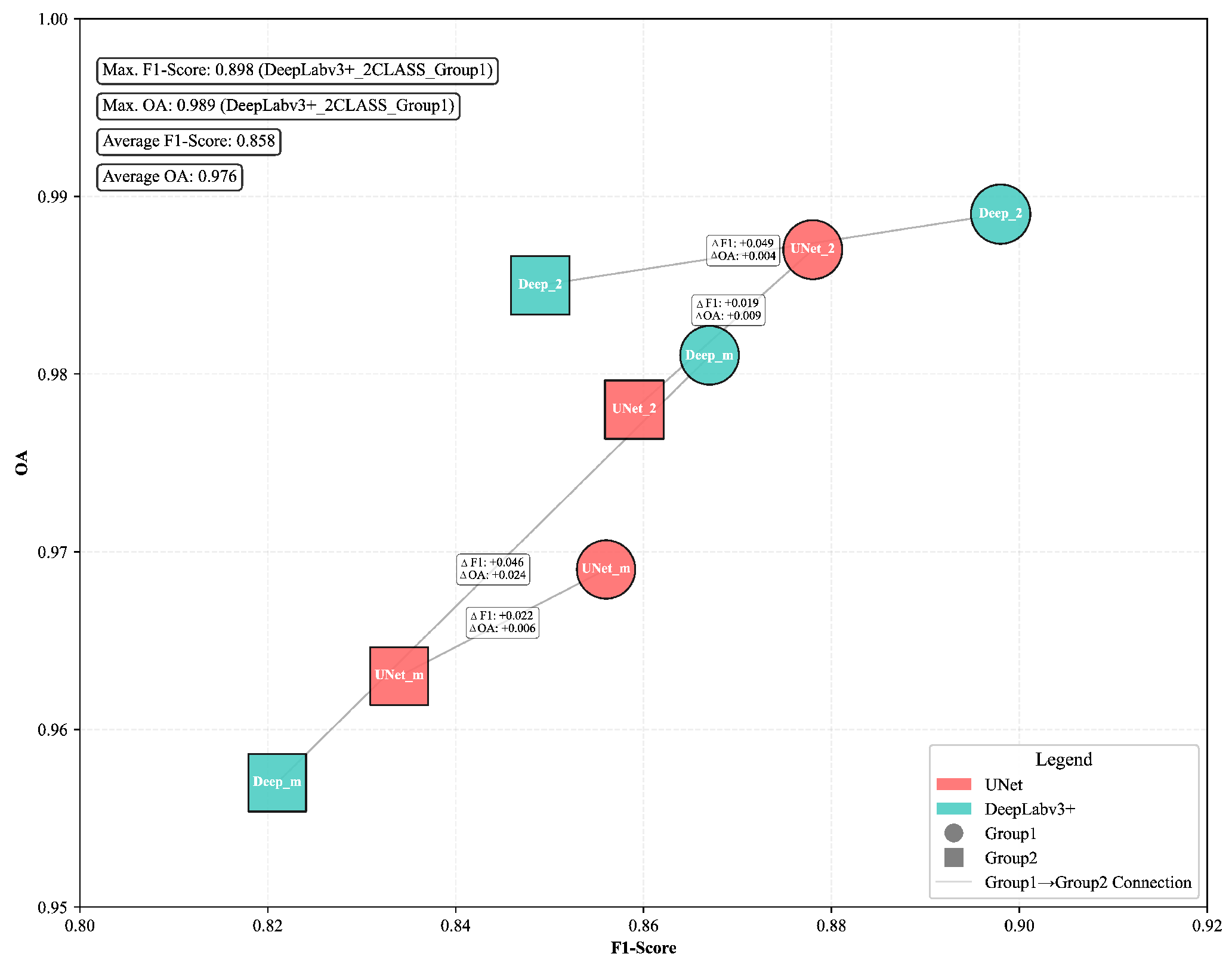
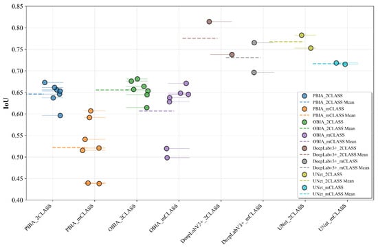
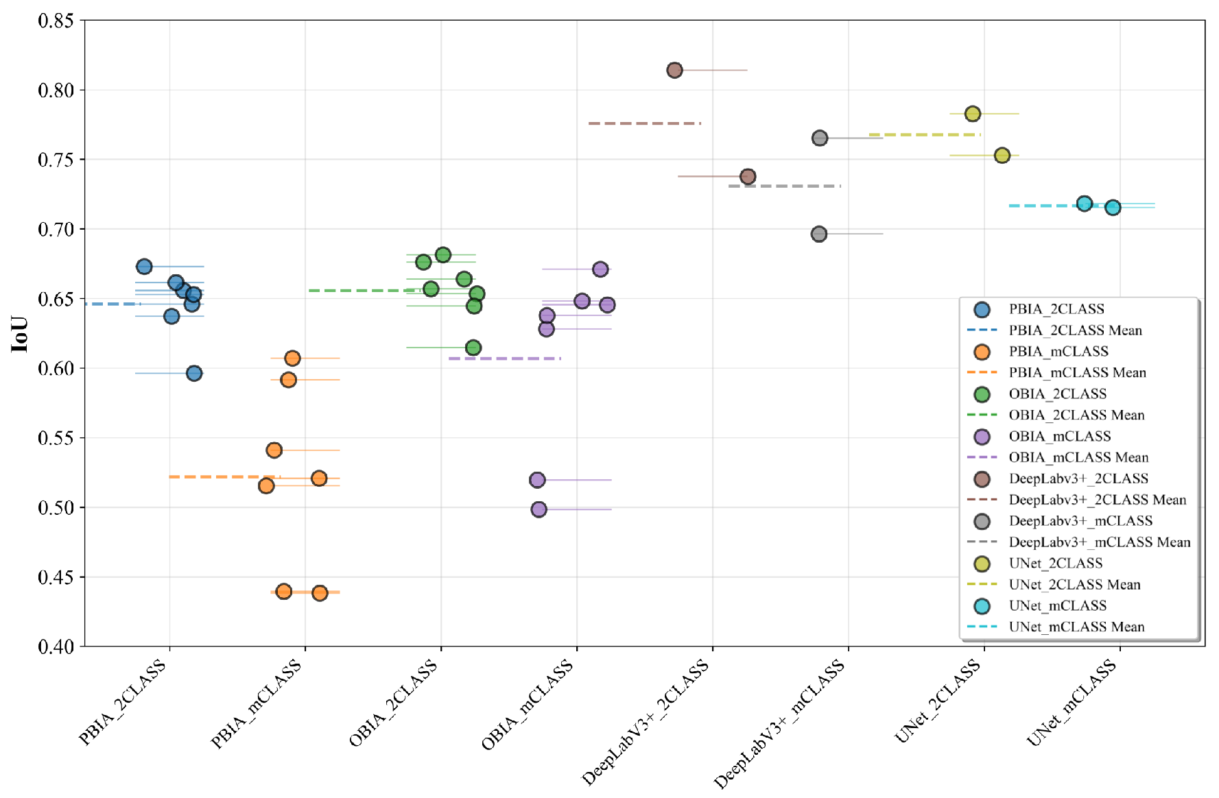
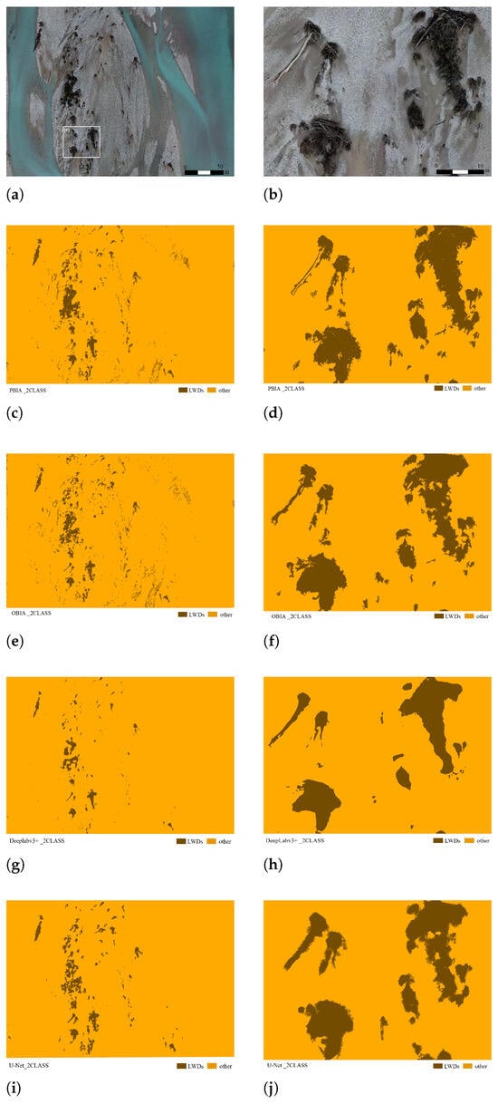
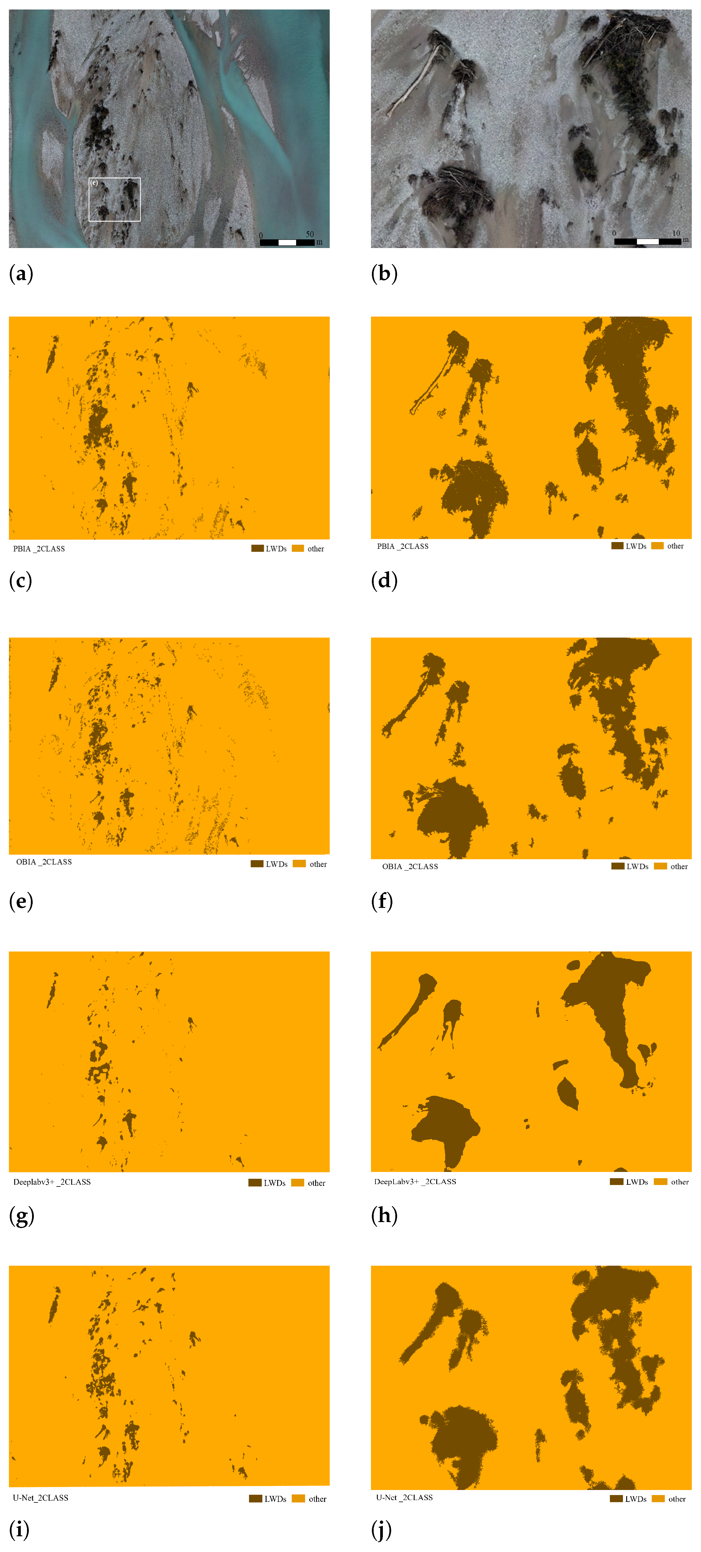
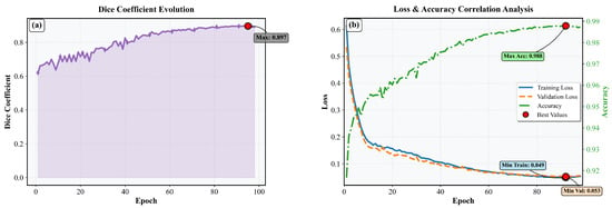
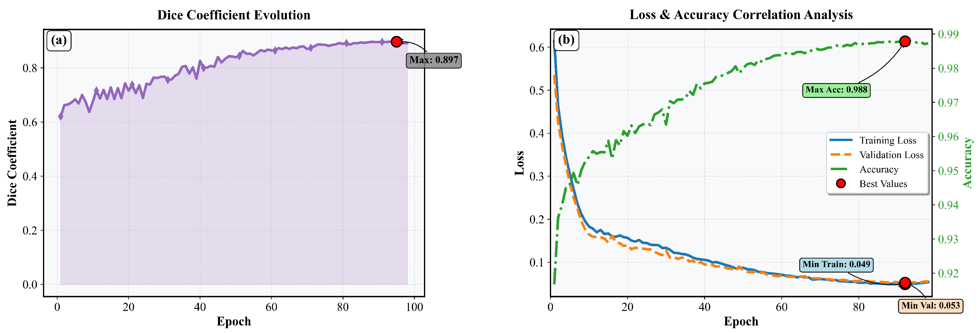
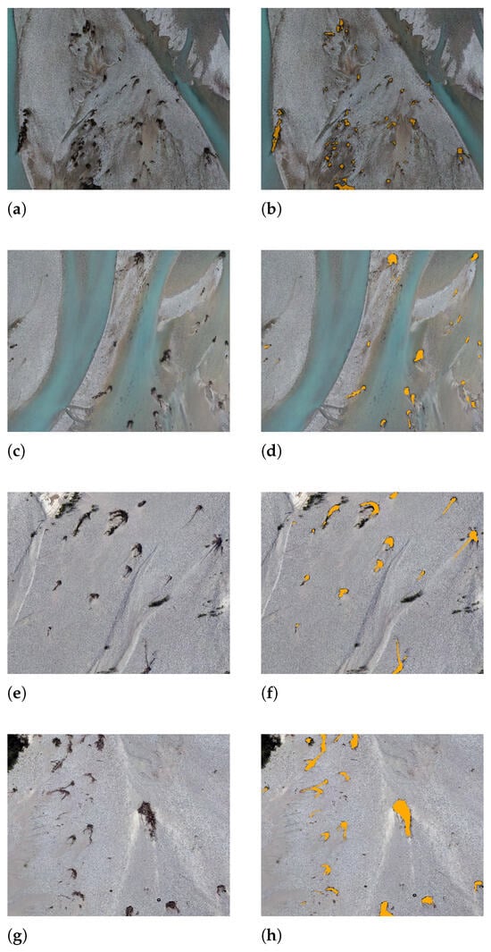
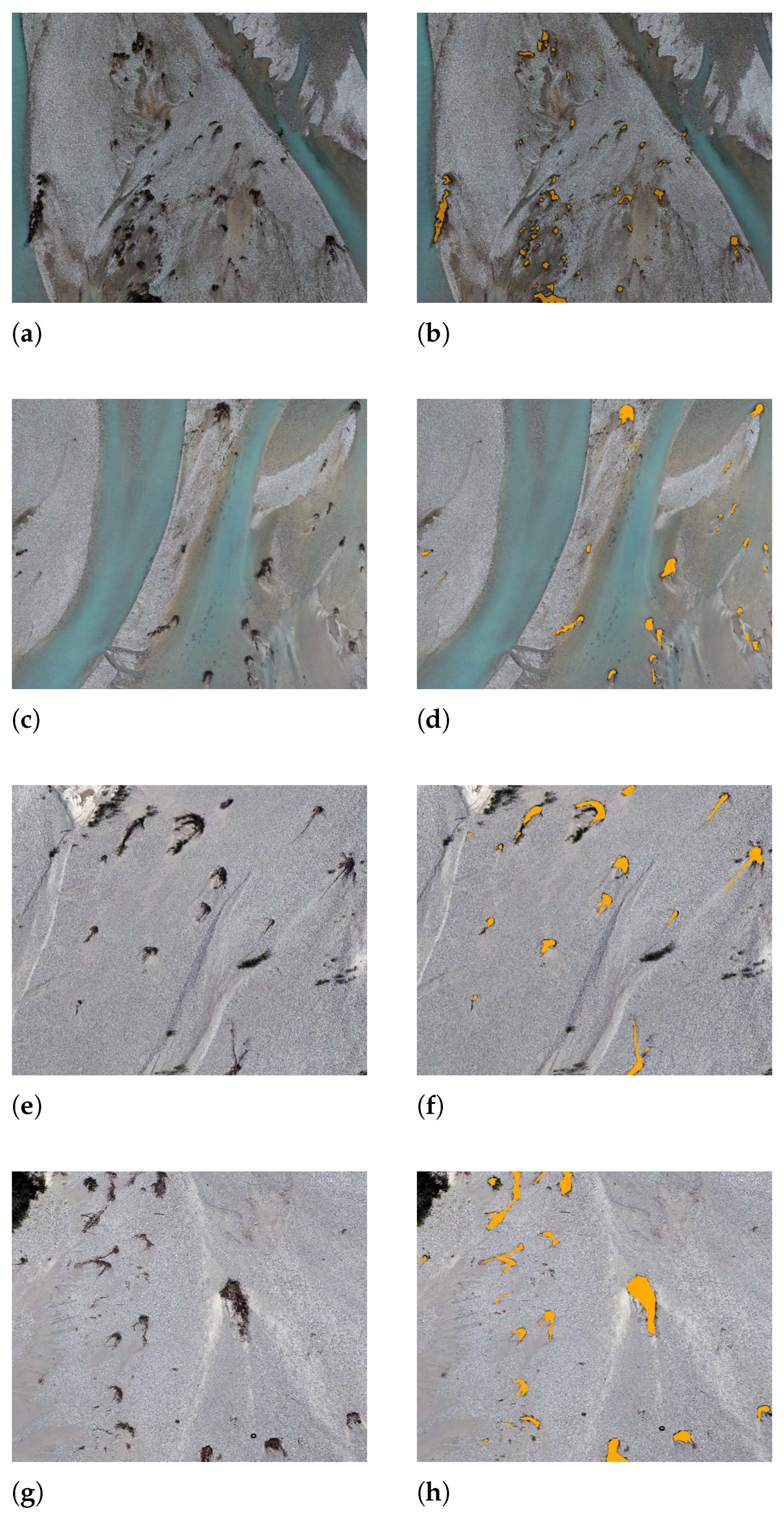
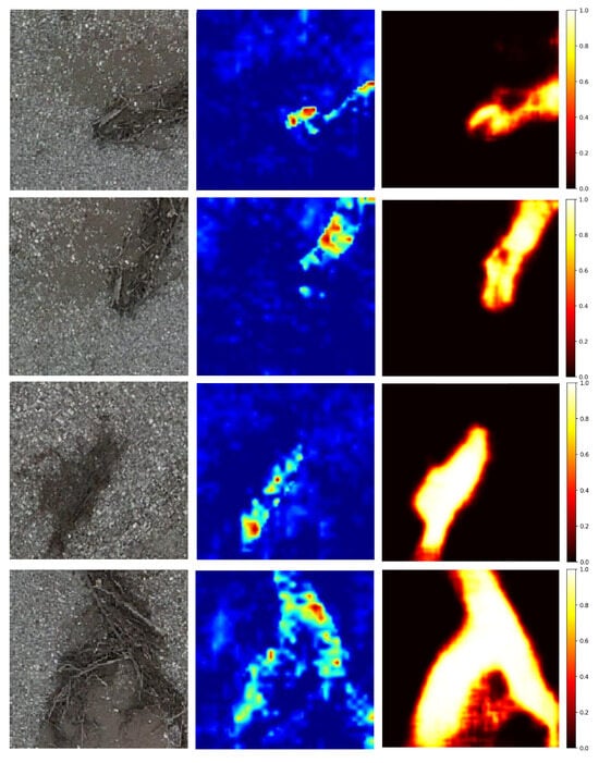
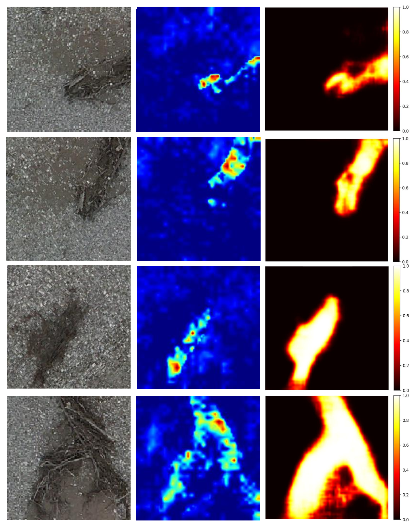

Disclaimer/Publisher’s Note: The statements, opinions and data contained in all publications are solely those of the individual author(s) and contributor(s) and not of MDPI and/or the editor(s). MDPI and/or the editor(s) disclaim responsibility for any injury to people or property resulting from any ideas, methods, instructions or products referred to in the content. |
© 2026 by the authors. Licensee MDPI, Basel, Switzerland. This article is an open access article distributed under the terms and conditions of the Creative Commons Attribution (CC BY) license.