A Process-Oriented Spatiotemporal Graph Framework for Analyzing Land-Cover Change from Remote Sensing Time Series

Highlights

What are the main findings?

• A geographical process object-based spatiotemporal graph (GPO-STG) framework was developed to model continuous land-cover change processes from remote sensing time series.
• Multilevel analysis of the NX-LCC-GPO-STG identified the key landscape processes, dominant interaction mechanisms, and sequential evolutionary patterns.

What are the implications of the main findings?

• The GPO-STG framework provides an effective and feasible alternative to conventional pixel- and object-based methods for characterizing complex spatiotemporal land-cover dynamics.
• The proposed multi-scale graph analysis confirms a “utilization–recovery” dynamic, revealing a dominant sequential transition from agricultural expansion to ecological restoration.

Abstract

Remote sensing time series (RSTS) are essential for monitoring land surface dynamics, yet existing pixel- or object-based methods often treat changes as isolated snapshots, failing to capture continuous spatiotemporal interactions. To address this, this study proposes the geographical process object-based spatiotemporal graph (GPO-STG) framework, which models land-cover changes as continuous geographical process objects (GPOs) connected by spatiotemporal topological relationships (STTRs). We applied this framework to the China Land Cover Dataset (CLCD) for the central arid and semi-arid region of the Ningxia Hui Autonomous Region (1991–2020) and conducted a systematic multilevel analysis. At the node level, degree centrality analysis identified key processes, revealing that grassland growing acts as the high centrality backbone of the regional landscape structure. At the edge level, interaction pattern analysis quantified the relationships between land-cover types and evolutionary states, uncovering a dominant coupling between grassland growing and cropland fluctuating. At the subgraph level, chain pattern extraction traced sequential evolutionary trajectories, confirming a “utilization–recovery” dynamic characterized by a transition from agricultural expansion to ecological restoration. The results demonstrate that the GPO-STG framework effectively characterizes complex land-cover changes that are often missed by pixel- or object-based methods.

1. Introduction

The Earth’s surface is a dynamic and complex system that undergoes continuous transformations due to various natural processes and human activities [1,2]. Remote sensing time series (RSTS) data holds immeasurable value for monitoring and analyzing the spatiotemporal patterns of Earth’s surface dynamics [3,4]. By providing sequential observations, RSTS data enable researchers to examine landscape dynamics across time, offering detailed insights into processes that drive changes [5,6,7].

RSTS data analysis methods can be categorized into two types: pixel-based [4,6,8,9,10,11] and object-based approaches [12,13,14]. While effective at quantifying the magnitude and location of change, these methods face a fundamental limitation: they treat landscape dynamics as a sequence of isolated states rather than continuous processes. Pixel-based methods lack spatial context, and while object-based methods incorporate spatial homogeneity [15], they still rely on comparing static snapshots. To enhance the semantic depth of these analyses, ontology-driven geographic object-based image analysis (O-GEOBIA) has emerged as a significant advancement [16]. By integrating formal knowledge representations, O-GEOBIA facilitates the transition from low-level pixels to high-level geographical entities with semantic meaning. This approach has proven particularly effective in characterizing complex ecological phenomena, such as forest-type mapping and the identification of ecological patterns [17,18], by providing a structured vocabulary for land-cover categories and their interrelationships. Furthermore, the connection between ontology and spatiotemporal graphs in a hierarchical structure allows for contextualizing landscape dynamics within the fundamentals of remote sensing hierarchy and topology [19,20]. However, even within an ontological framework, capturing the fluidity of processes remains a challenge. Consequently, they fail to capture the underlying spatiotemporal interactions among evolving objects [21,22]. For instance, how an ecological restoration process in one area might drive or constrain land-cover fluctuations in its neighborhood.

To address relational complexity, graph-based RSTS analysis has gained attention [23,24,25]. Early pioneering work by Cheung et al. [26] demonstrated the superiority of graph theory over traditional data lattices for landscape monitoring. Building upon this foundation, researchers have proposed methods for linking spatial objects over time to enable in-depth temporal analysis [27], enhanced graph simplification and clustering algorithms [28,29], and spatiotemporal structural graph techniques for comprehensive land-cover change analysis [30]. Moreover, methods for extracting spatial roles, adjacency types, temporal transitions, and evolution trajectories have been proposed [31,32]. Advanced models, such as hybrid spatiotemporal graph convolutional networks, have been introduced to capture complex interactions between landscape elements [33], and state-and-evolution detection models facilitate continuous detection of long-term evolution patterns [34,35].

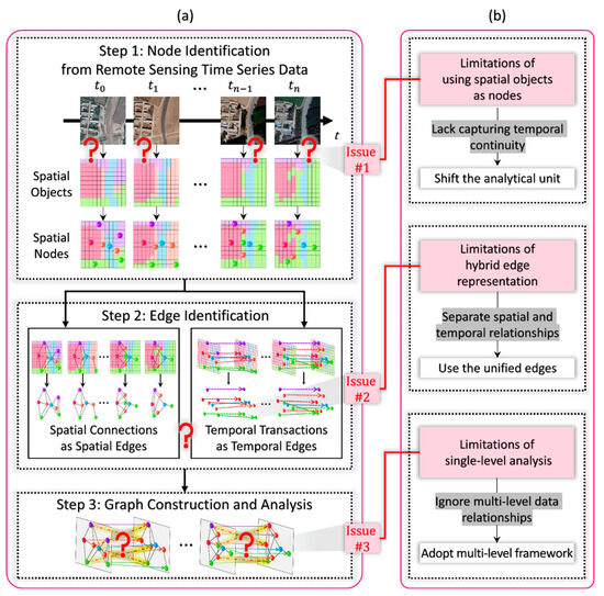
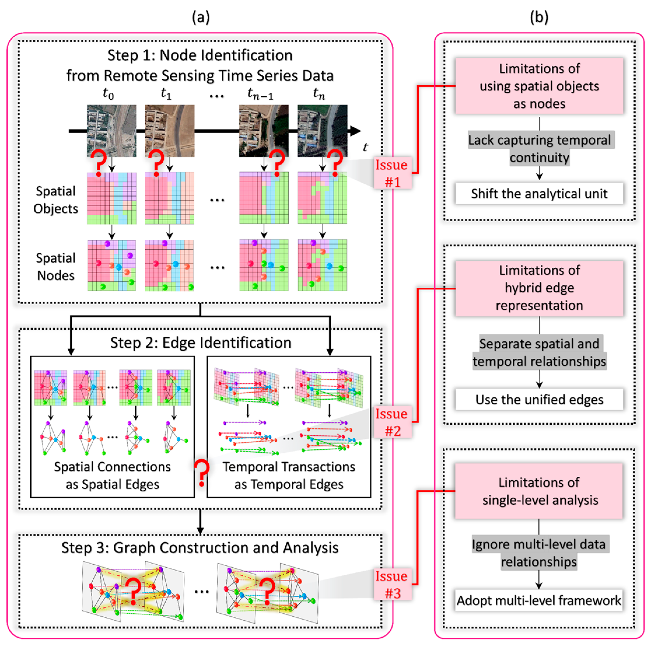
However, existing graph methods often adopt a “divide-and-conquer” strategy that fragments the spatiotemporal continuity of geographical processes. As illustrated in Figure 1a, typical graph-based RSTS workflows involve three main steps: (1) extracting spatial objects as nodes from each time step in RSTS data, (2) establishing spatial connections as spatial edges and temporal transitions as temporal edges, and (3) forming a spatiotemporal graph by linking nodes using a combination of undirected spatial edges and directed temporal edges [36,37]. This fragmentation results in three specific limitations, as summarized in Figure 1b.

Figure 1. Concepts, limitations and solutions of current graph-based RSTS data analysis methods: (a) three steps of current methods; (b) identified limitations (pink), core issues (gray), and potential solutions (white).

Limitations of using spatial objects as nodes: Existing methods handle RSTS data frame by frame, segmenting each image into spatial objects. Although these spatial objects exhibit spatial homogeneity and connectivity, they lack temporal considerations and fail to capture the inherent spatiotemporal heterogeneity and autocorrelation of geographical phenomena [38,39]. To address this, guided by principles of process-based spatiotemporal analysis [40], we hypothesize shifting the analytical unit from static spatial objects to geographical process objects (GPOs). GPOs are continuous in both space and time and represent Earth’s surface processes throughout their entire lifecycle [41]. This process-based approach may offer a more integrated perspective of the Earth’s surface dynamics.

Limitations of hybrid edge representation: Current graph-based RSTS analysis methods combine directed temporal edges and undirected spatial edges [3]. This hybrid representation introduces analytical constraints by treating spatial connections and temporal transitions as independent aspects [42]. We consider another hypothesis: we use a unified edge representation embedded with spatiotemporal attributes instead. By adopting this unified approach, all analyses are based on edges that inherently capture both spatial and temporal relations, eliminating fragmentation and simplifying the spatiotemporal graph.

Limitations of single-level analysis: Owing to the distinction between temporal and spatial edges, existing methods focus on capturing spatial dependencies between objects at a single time or temporal dependencies of the same object across time. This single-level focus overlooks the intricate multilevel spatiotemporal relations embedded within the data, such as interactions at the subgraph or global levels and emergent patterns arising from the collective behavior of multiple objects [43]. By overlooking these relations at different levels, current methods fail to capture the full complexity of Earth’s system processes. Informed by multilevel analysis theory [44], we hypothesize an analytical framework that examines a graph across multiple levels (node, edge, and subgraph), enabling a layered understanding of spatiotemporal dynamics [45].

Based on these hypotheses, we propose the geographical process object-based spatiotemporal graph (GPO-STG) framework. This framework introduces three key shifts: (1) shifting the analytical unit to GPOs, entities that represent the continuous lifecycle of Earth’s surface processes [41]; (2) employing a unified edge representation embedded with spatiotemporal attributes to explicitly model interactions; and (3) adopting a multilevel analysis to reveal dynamics from local to global patterns. We apply this framework to the central arid and semi-arid region of the Ningxia Hui Autonomous Region using the China Land Cover Dataset (CLCD) [46] to validate the capability of GPO-STG.

2. Materials and Methods

2.1. Study Area and Data

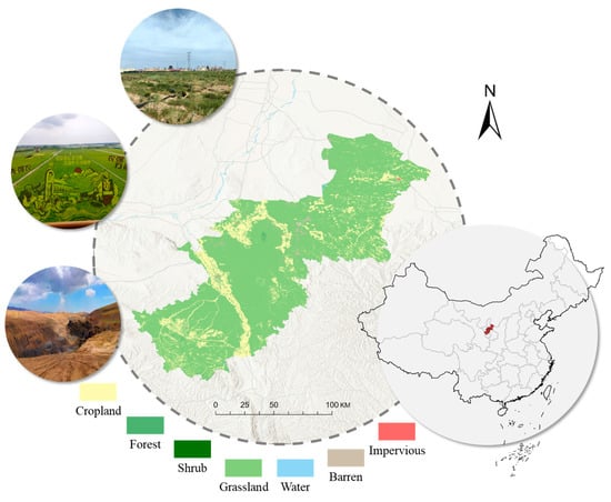
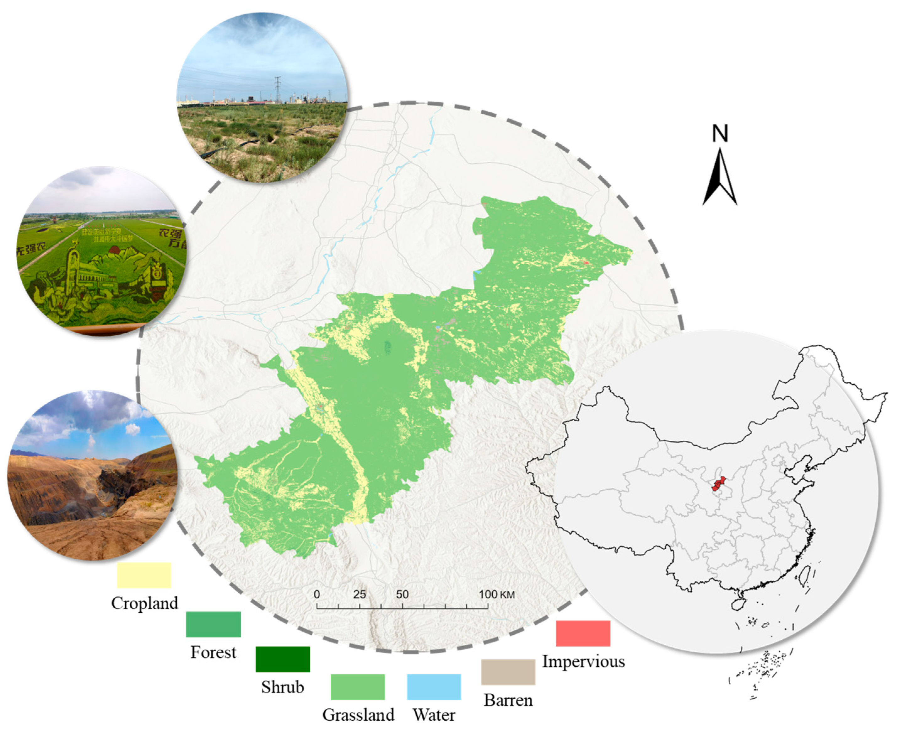
The study focuses on the central arid and semi-arid region of the Ningxia Hui Autonomous Region (as shown in Figure 2), ranging from 104°17′E to 107°39′E and from 36°00′N to 38°10′N. Situated in the agro-pastoral ecotone of Northern China, the region transitions between the Loess Plateau and the Tengger Desert. This typical ecologically fragile zone is characterized by a temperate continental monsoon climate with intense evaporation and sparse vegetation, rendering the ecosystem highly sensitive to both climatic variations and human activities. The landscape features a complex mosaic of cropland, forest, shrub, grassland, water, barren land, and impervious surfaces. Natural vegetation is dominated by dry and desert steppes, while agriculture primarily relies on dryland farming, supplemented by “Yanghuang” (Yellow River lifting) and well irrigation. Since the late 1990s, the region has undergone significant land-cover transformations driven by major ecological projects, including the “Three-North Shelterbelt”, “Grain for Green”, and ecological migration programs. These interventions have profoundly altered regional landscape patterns through water resource regulation, land use management, and ecosystem restructuring.

Figure 2. Study area.

This study leverages the CLCD [46], which provides continuous annual land-cover classifications from 1985 onward at a high spatiotemporal resolution. It provides detailed categorization, including the categories of cropland, forest, shrub, grassland, water, snow/ice, barren, impervious surface, and wetland. CLCD enables the detection of fine-scale landscape fragmentation and inter-annual dynamics, serving as the basis for GPO extraction. Specifically, we utilize CLCD data covering central Ningxia from 1991 to 2020 as the direct input for spatiotemporal cube segmentation and graph construction.

2.2. Identifying and Characterizing GPOs

2.2.1. GPO Identification Using Spatiotemporal Cube Segmentation

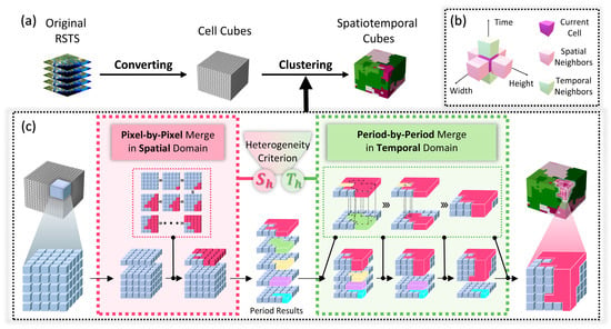
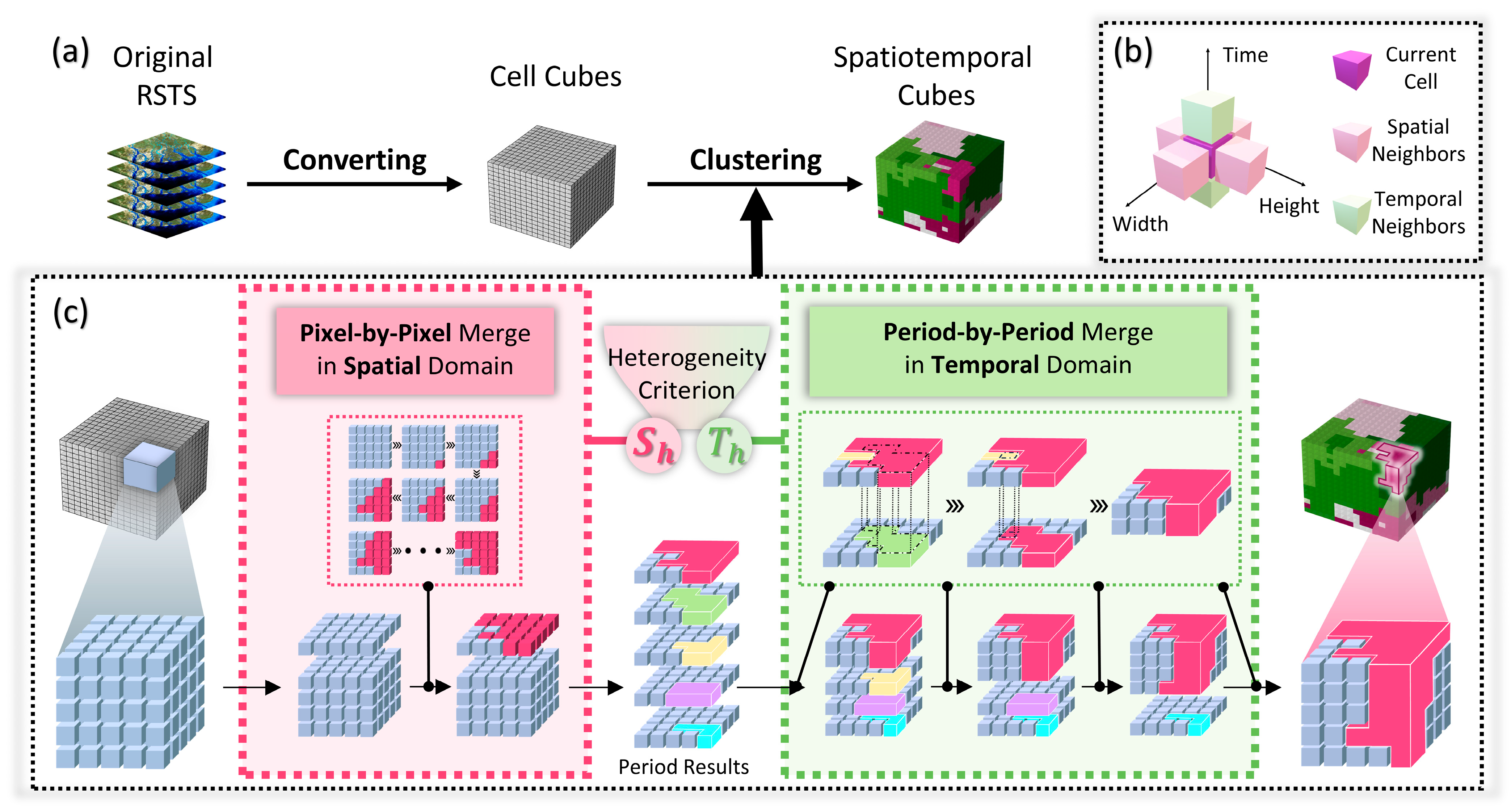
GPOs are extracted using a spatiotemporal cube segmentation method that partitions RSTS data into continuous spatiotemporal cubes, each capturing a distinct process across both space and time (Figure 3a). Each cube represents a segment of a GPO within a contiguous region, maintaining continuity in both the space and time dimensions. For each spatiotemporal cube, potential merging candidates are identified based on their spatiotemporal neighbors, classified as spatial or temporal (Figure 3b). Spatial neighbors are cubes directly adjacent in space with overlapping temporal periods, whereas temporal neighbors are adjacent in time with overlapping spatial regions. As shown in Figure 3c, the spatial clustering rule $S_h$ is first applied to perform pixel-by-pixel merging in the spatial domain. Subsequently, the temporal clustering rule $T_h$ is applied to perform period-by-period merging in the temporal domain. The specific mathematical formulation for the heterogeneity criterion is detailed in Appendix A. Specifically, the heterogeneity thresholds for both $S_h$ and $T_h$ were set to zero, enforcing strict label consistency where a merge operation is executed if and only if the subject cube and its spatiotemporal neighbors possess an identical land-cover class code. This ensures that each identified GPO represents a spatially and temporally continuous entity of a single land-cover type.

Figure 3. GPO identification using spatiotemporal cube segmentation: (a) conversion of data into 3D voxels as cell cubes and clustering based on predefined rules to generate spatiotemporal cubes, (b) concept of spatiotemporal neighbors, (c) merging process for spatial (pixel-by-pixel) and temporal (period-by-period) domains using heterogeneity criterion.

2.2.2. Multi-Dimensional Feature Representation of GPOs

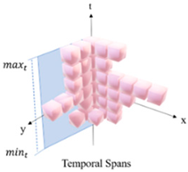
The multi-dimensional characteristics of GPOs are categorized into three domains: location, morphology, and evolution. Collectively, these dimensions comprehensively characterize the spatiotemporal attributes and dynamics of GPOs by addressing “where they are”, “what form they take”, and “how they evolve”. Specifically, location features provide explicit spatiotemporal positioning, defining the fundamental boundaries of the object within the spatial and temporal domains. Morphological features quantify their geometric shape and complexity within the 3D space, capturing structural variations in the object’s external form across different timestamps. Evolutionary features, centered on the temporal dimension, reveal dynamic trends and patterns, characterizing processes such as expansion, contraction, or fluctuation over specific periods. Detailed definitions and calculation methods for these features are provided in Appendix B.

2.3. Establishing and Characterizing STTRs Among GPOs

2.3.1. STTR Establishment Using Spatiotemporal Topology Computation

The interactions and connections between GPOs are analyzed in detail in this study using STTRs as a distinguishing tool. Spatiotemporal topology effectively represents the interactions and connections among GPOs across spatial and temporal dimensions [47,48]. They establish a comprehensive framework for analyzing how GPOs are positioned and evolve within a multi-dimensional continuum, integrating both temporal and spatial dynamics. For robust analyses of GPOs within specified temporal and spatial constraints [49], the interplay between temporal topology (transition of objects over time) and spatial topology (connection of objects in space) should be considered [50].

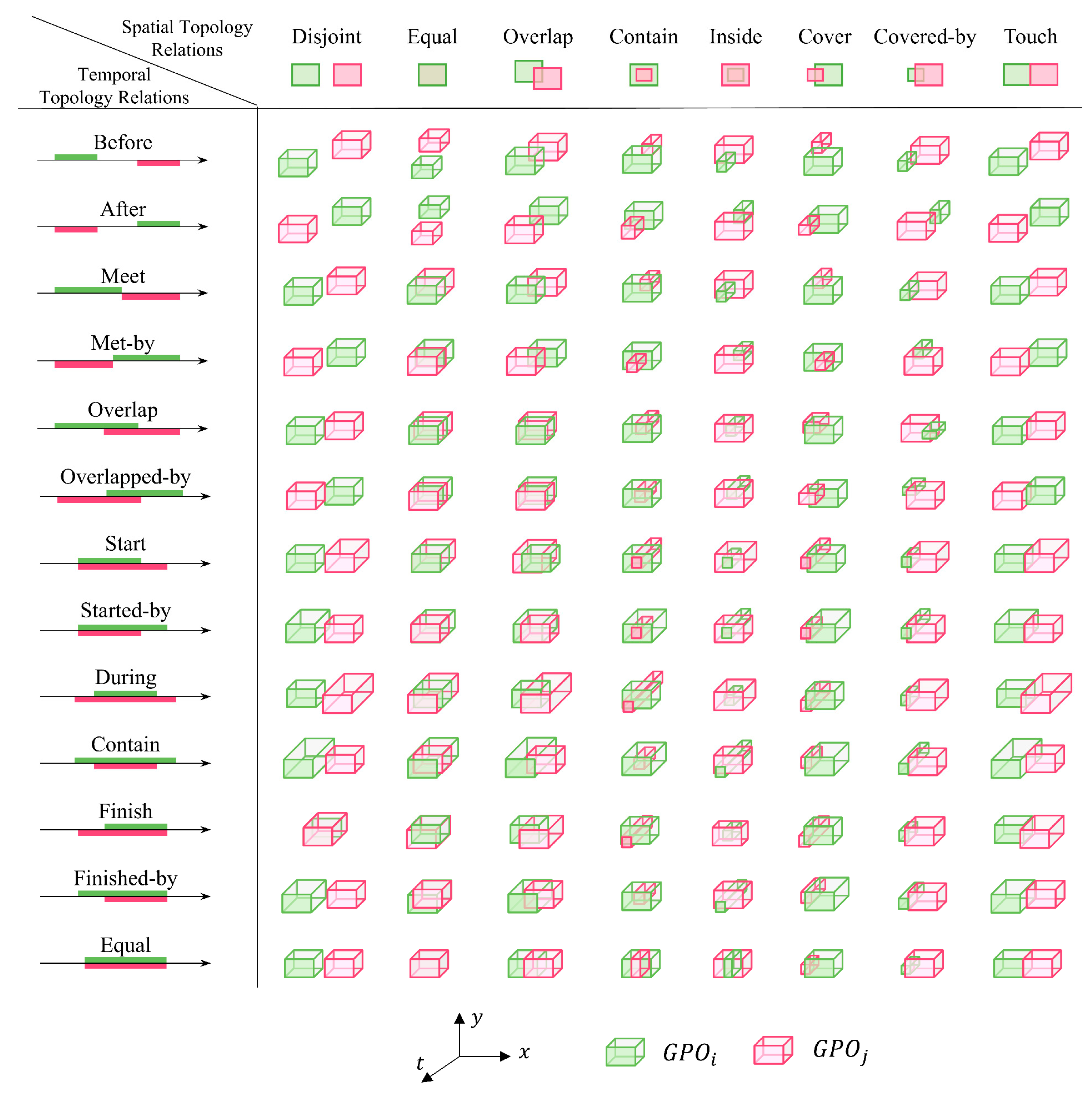
Temporal topology relations, as defined by Allen’s interval algebra [51], provide a systematic framework for categorizing the relative positions and sequences between time intervals into 13 distinct types: before, after, meets, met by, overlaps, overlapped by, during, contains, starts, started by, finishes, finished by, and equal. Spatial topology relations, which delineate the arrangement of two GPOs in space [52], are classified into 8 distinct types: disjoint, equal, overlap, contain, inside, cover, covered by, and touch. Theoretically, these combine to form 104 distinct spatiotemporal topological relations.

Although these 104 combinations provide a complete theoretical framework, a simplified scheme based on 3D voxel adjacency was adopted for the practical analysis in this study. In this scheme, an edge is defined as a physical contact relationship between two GPOs within the 3D spatiotemporal array, representing coplanarity. This simplified approach focuses on the direct physical interaction between GPOs, determined by retrieving heterogeneous neighboring voxels across the temporal and spatial axes. They are mathematically expressed in Appendix C.

2.3.2. Quantitative Representation of STTRs

Following the qualitative description of spatiotemporal topological relations, it is necessary to translate these relationships into quantifiable metrics to deeply analyze the interaction mechanisms between GPOs. Accordingly, this study quantifies spatiotemporal topological relations using four dimensions: distance, azimuth, degree of overlap, and connection intensity.

(1)

Distance

Let ($x_i,y_i,t_i$) and ($x_j,y_j,t_j$) denote the spatiotemporal centroids of ${GPO}_i$ and ${GPO}_j$, respectively. The Euclidean distance between them is defined as Equation (1). This metric quantifies the overall distributional divergence of two GPOs within the spatiotemporal coordinate system, where a smaller distance indicates greater proximity in space-time.

$$d_{ij}=\sqrt{{\left(x_j-x_i\right)}^2+{\left(y_j-y_i\right)}^2+{\left(t_j-t_i\right)}^2}$$

(1)

(2)

Azimuth

Let ${\theta }_{\mathrm{i}}$ and ${\theta }_{\mathrm{j}}$ represent the overall orientation vectors of ${GPO}_i$ and ${GPO}_j$, respectively. The directional difference is defined as Equation (2). This azimuth metric reflects the deviation of the GPOs relative to the time axis in the spatiotemporal graph; a smaller directional difference implies a higher consistency in their evolutionary trajectories.

$${\theta }_{ij}=\left\{\begin{array}{c}\left|{\theta }_i-{\theta }_j\right|\\ 360°-\left|{\theta }_i-{\theta }_j\right|\end{array}\right.$$

(2)

(3)

Degree of Overlap

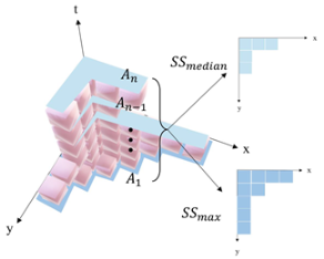
To quantify interaction within the spatiotemporal domain, we utilize both spatial projection overlap and temporal span overlap. Let $A_{median}$ and $A_{max}$ represent the median and maximum projection areas of the GPOs at different timestamps, respectively; and let $TS\left({GPO}_i\right)$ and $TS\left({GPO}_j\right)$ represent their respective temporal spans. The degree of overlap ($O_{ij}$) is defined as Equation (3):

$$O_{ij}=\alpha \times \left({\displaystyle \frac{A_{median}\left({GPO}_i\right)\cup A_{median}\left({GPO}_j\right)}{A\left({GPO}_i\right)+A\left({GPO}_j\right)}}\right)+\beta \times \left({\displaystyle \frac{A_{max}\left({GPO}_i\right)\cup A_{max}\left({GPO}_j\right)}{A\left({GPO}_i\right)+A\left({GPO}_j\right)}}\right)+(1-\alpha -\beta )\times \left({\displaystyle \frac{TS\left({GPO}_i\right)\cup TS\left({GPO}_j\right)}{TS\left({GPO}_i\right)+TS\left({GPO}_j\right)}}\right)$$

(3)

Here, $\alpha$ and $\beta$ are weight coefficients. In this study, an equal weighting strategy ($\alpha =\beta ={\displaystyle \frac{1}{3}}$) is adopted, assuming that spatial coverage and temporal persistence contribute equally to the interaction intensity. This heuristic balance avoids a priori bias and allows the framework to simultaneously capture diverse dynamics, such as instantaneous intense changes and long-term subtle variations. This metric provides a comprehensive assessment of spatiotemporal interaction, where a higher value indicates a greater degree of overlap.

(4)

Connection Intensity

Based on the centroid distance, the connection intensity ($I_{ij}$) is defined as Equation (4). A smaller centroid distance yields a higher connection intensity, indicating a tighter spatiotemporal interaction or a higher potential for interplay between the two GPOs.

$$I_{ij}={\displaystyle \frac{1}{{\mathrm{d}}_{ij}}}$$

(4)

2.4. Construction and Analysis of GPO-STG

2.4.1. Construction of the GPO-STG

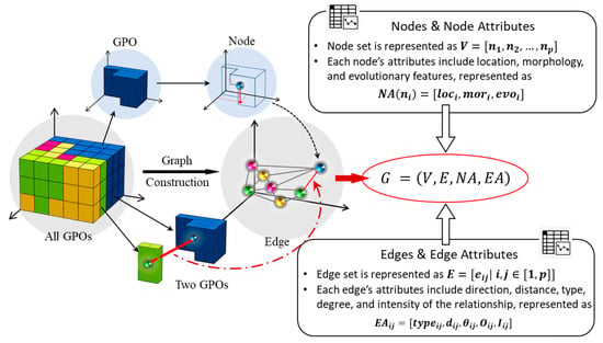
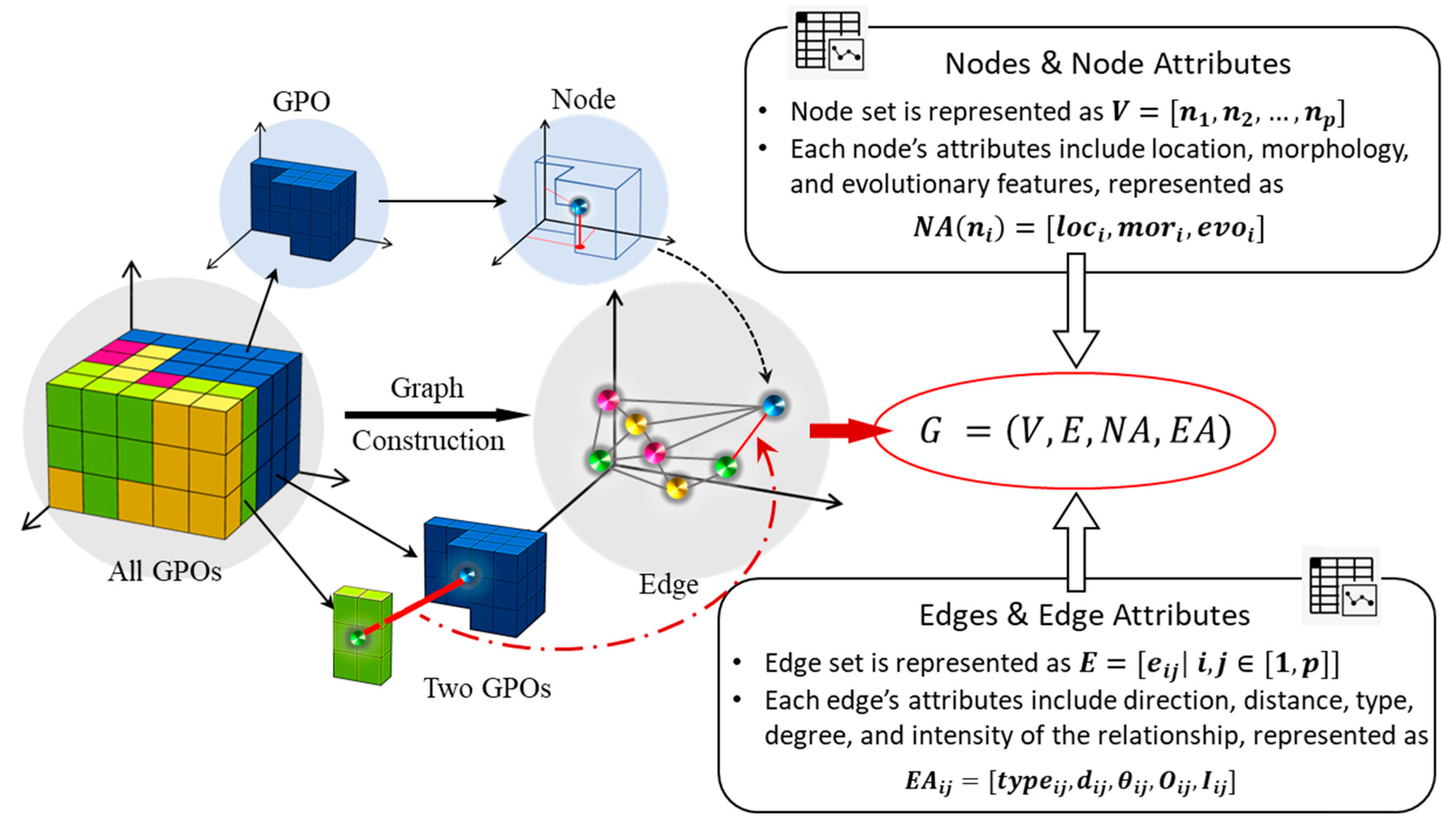
To systematically quantify the complex interactions within RSTS, we developed the GPO-STG framework. As shown in Figure 4, the GPO-STG maps the identified GPOs and their interactions into a graph structure. The construction process consists of three main steps. First, each GPO in the global set is abstracted as a node $n_i$ within the node set V. These nodes are assigned attributes $NA\left(n_i\right)=[{loc}_i,{mor}_i,{evo}_i]$ representing their spatial location, morphology, and evolutionary characteristics. Second, the interactions between any two GPOs are evaluated to determine the presence of an edge $e_{ij}$ in the edge set $E$. An edge is established if a spatiotemporal relationship is identified, with corresponding attributes ${EA}_{ij}=[{type}_{ij},{d_{ij},{\theta }_{ij},O}_{ij},I_{ij}]$ quantifying the strength and nature of the interaction. Finally, these components are integrated into the formal graph structure, formally defined as a quadruple (Equation (5)):

$$G=(V,E,NA,EA)$$

(5)

where V (nodes) represents the set of identified GPOs. E (edges) represents the set of STTRs between nodes. NA (node attributes) is denoted as $NA\left(n_i\right)=[{loc}_i,{mor}_i,{evo}_i]$; these attributes describe the intrinsic spatiotemporal characteristics of each GPO (Section 2.2.2). EA (edge attributes) is denoted as ${EA}_{ij}=[{type}_{ij},{d_{ij},{\theta }_{ij},O}_{ij},I_{ij}]$; these attributes quantify the strength and nature of the interactions (Section 2.3.2).

Figure 4. The construction workflow of the GPO-STG framework, illustrating the transformation of all identified GPOs into nodes $V$ with attributes $NA$ and the evaluation of interactions between two GPOs to establish edges $E$ with attributes $EA$.

2.4.2. Analysis of the GPO-STG

We implemented a multilevel analysis framework to interpret the GPO-STG from three perspectives: the node level (investigating individual roles and centrality), the edge level (analyzing interaction mechanisms and transitions), and the subgraph level (identifying local evolutionary motifs).

(1)

Node-Level Analysis

We employ degree centrality to evaluate the centrality of specific land-cover process. Degree centrality measures the number of direct interactions a geographic process object has with its neighbors. It reflects the immediate influence of a node within the graph. Let $deg\left(v\right)$ be the number of edges connected to node $v_i$ and $N$ be the total number of nodes in the graph. The degree centrality $C_D\left(v_i\right)$ is defined as Equation (6):

$$C_D\left(v_i\right)={\displaystyle \frac{deg\left(v_i\right)}{N-1}}$$

(6)

(2)

Edge-Level Analysis

To systematically characterize node interactions, we propose three categories of edge-level analysis patterns based on structural graph queries: land-cover type, evolutionary state, and composite attribute interactions. Land-cover type interaction maps adjacency relationships between distinct land-cover classifications. By quantifying specific edge combinations (e.g., “cropland–shrub”), this analysis may reveal direct spatial linkages and potential conversion pathways between different categories. Evolutionary state interaction investigates temporal dynamics by identifying state-transition motifs (e.g., “stable–growing” or “fluctuating–fluctuating”). Analyzing the frequency and distribution of these pairings may elucidate co-evolutionary characteristics and the propagation mechanisms of dynamic changes across the landscape. Composite attribute interaction integrates both land-cover type and evolutionary states to capture complex synergies. By examining interactions between composite node attributes (e.g., “grassland growing–barren stable”), this approach may uncover the underlying multi-dimensional logic driving land-cover change.

(3)

Subgraph-Level Analysis

Subgraph extraction isolates subsets with specific structures from the complete graph to identify local network features. We specifically utilize chain patterns to identify sequential evolutionary processes. These patterns may reveal the cascading effects of land-cover transformation. Methodologically, we employ a strategy combining breadth-first traversal with bidirectional neighborhood search. The chain pattern detection process begins by traversing all existing edges $(a,b)$ in the spatiotemporal graph. For each identified edge, the algorithm extracts the neighborhood of the target node $b$. To ensure the directionality of the chain and avoid cycles, any reverse connections pointing back to the starting node $a$ are explicitly removed from this neighborhood set. Let $N\left(b\right)$ denote the valid neighbor set of $b$. We then construct a set of candidate triples defined as $\left[\right(a,b,c)\mid c\in N(b\left)\right]$. Subsequently, a temporal constraint is applied to each candidate triple to ensure the logical sequence of evolution. Let ${STC}_{t_a}$, ${STC}_{t_b}$ and ${STC}_{t_c}$ represent the spatiotemporal center times of nodes $a$, $b$, and $c$, respectively. A valid chain pattern is identified only if the nodes satisfy the following strict sequential condition, namely ${STC}_{t_a}<{STC}_{t_b}<{STC}_{t_c}$. Finally, the algorithm outputs all triples satisfying these requirements.

3. Results

Using the CLCD data spanning the period of 1991 to 2020, we constructed the GPO-STG for the land-cover change analysis in the central arid and semi-arid of the Ningxia Hui Autonomous Region (hereinafter referred to as NX-LCC-GPO-STG). Based on the NX-LCC-GPO-STG, we conducted a systematic multilevel analysis to uncover the spatiotemporal dynamics of the regional landscape. First, we characterize the overall graph characteristics and visualize the spatiotemporal complexity of the land-cover changes (Section 3.1). Subsequently, we identify the key processes acting as the backbone of the landscape structure through node centrality analysis (Section 3.2). We then investigate the interaction mechanisms between land-cover types and evolutionary states at the edge level (Section 3.3). Finally, we reveal the sequential evolutionary trajectories and the “utilization–recovery” dynamic patterns through subgraph chain analysis (Section 3.4).

3.1. Graph Characteristics of Land-Cover Change in Ningxia

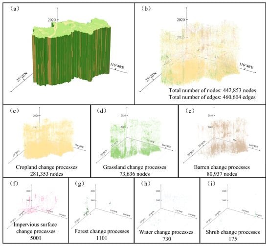
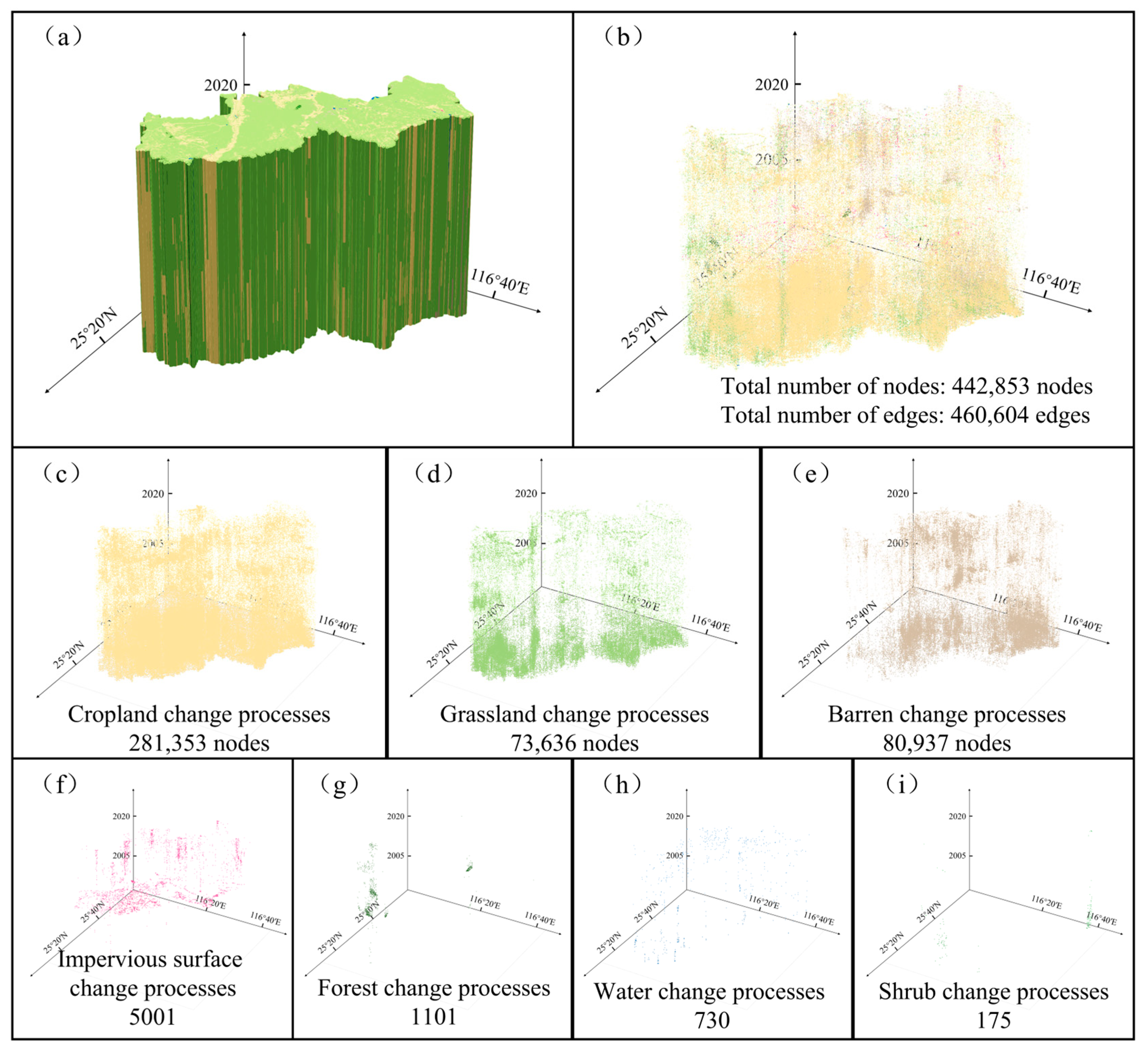
The constructed NX-LCC-GPO-STG reveals a highly complex high-dimensional network structure, comprising 442,852 process nodes and 460,604 interaction edges. The three-dimensional spatiotemporal cube visualization in Figure 5a intuitively depicts the spatiotemporal trajectories of land-cover change in the arid and semi-arid region of Central Ningxia from 1991 to 2020. The vertical axis represents temporal evolution, while the planar coordinates denote geographic location; the intertwined network of lines vividly illustrates the transition pathways of specific land parcels between different land-cover types over time. Figure 5b displays the resulting complete spatiotemporal graph structure, where its highly dense connectivity reflects extensive and complex spatiotemporal entanglement among land-cover change processes within the study area. Figure 5c–i further reveal structural disparities among the change processes of different land-cover types. A prominent feature is that the process graphs for cropland (Figure 5c), grassland (Figure 5d), and barren land (Figure 5e) exhibit extremely high node density and widespread spatial distribution. In contrast, the process graphs for impervious surfaces (Figure 5f), forest (Figure 5g), water bodies (Figure 5h), and shrubland (Figure 5i) appear relatively sparse and localized.

Figure 5. Spatiotemporal graph of land-cover change process in the arid and semi-arid region of Central Ningxia from 1991 to 2020. (a) Continuous evolutionary processes in the 3D spatiotemporal cube; (b) the constructed spatiotemporal graph structure; (c–i) detailed visualization of change processes for cropland, grassland, barren, impervious surfaces, forest, water, and shrub.

These graph characteristics are not merely descriptive statistics, but hold significant geospatial and methodological implications. The sheer scale of 442,852 process nodes and 460,604 interaction edges quantifies the complexity of the landscape dynamics that traditional pixel-based or object-based change detection methods typically fail to capture. Conventional approaches often analyze changes as discrete, independent events or patches, treating a conversion from grassland to cropland, for instance, as an isolated occurrence. In contrast, the GPO-STG method constructs a unified topological network where each node is a unique spatiotemporal process and each edge represents a potential interaction or adjacency. This structure allows us to move beyond simple change matrices and reveal the systemic property of landscape evolution. The highly dense connectivity observed, particularly for cropland, grassland, and barren land, signifies that these are not merely the most abundant land-cover types but constitute the structural matrix of change, acting as hubs within the network of landscape dynamics. This finding, which would be impossible to derive from traditional methods lacking a spatiotemporal topological framework, demonstrates that landscape changes in this arid region are highly structured and ecologically organized, rather than randomly distributed.

3.2. Node-Scale Analysis for Identification of Key Processes

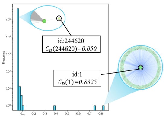
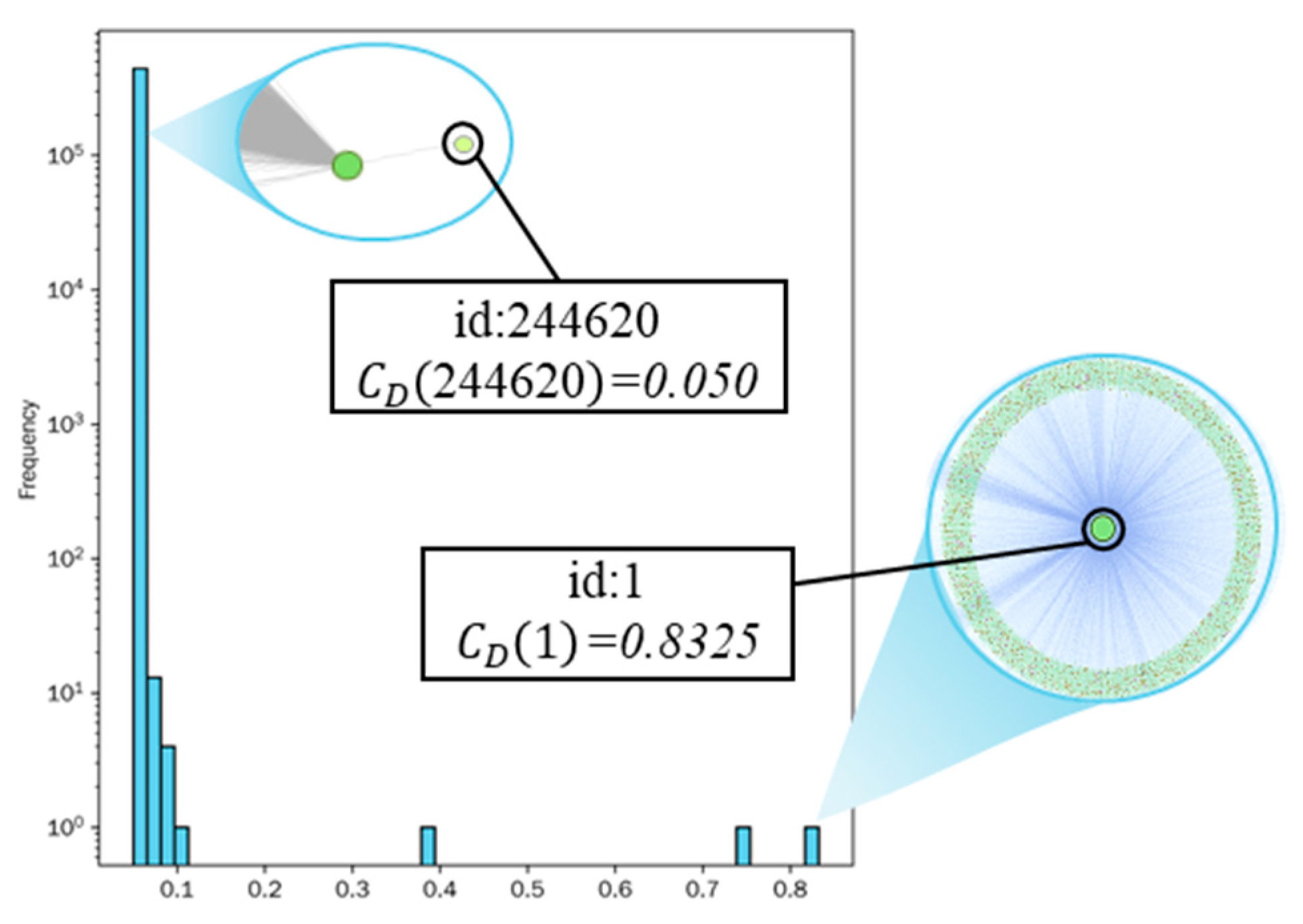
The distribution of degree centrality for all nodes within the NX-LCC-GPO-STG evaluates the influence of specific land-cover change processes. As illustrated in Figure 6, the results exhibit a pronounced heavy-tailed distribution characteristic. To clarify the structural differences between typical processes, the figure includes magnified callouts of nodes with contrasting centrality levels. Specifically, the vast majority of nodes in the graph possess extremely low centrality values under 0.1, representing isolated change processes characterized by small spatial extents or marginal locations. For instance, node 244620 exhibits a low degree centrality of 0.050, indicating limited interaction with other processes. In contrast, a select few nodes demonstrate exceptionally high connectivity.

Figure 6. Statistical distribution and topological visualization of node degree centrality in the NX-LCC-GPO-STG, where the histogram shows a heavy-tailed distribution and the inset callouts contrast an isolated process (node 244620) with a central backbone process (node 1).

Quantitative analysis identifies processes such as the long-term grassland growing process at the head of the distribution. This is exemplified by node 1, which maintains a degree centrality as high as 0.8325 and acts as a central hub connecting numerous surrounding processes. These processes are characterized by large spatial extents and long durations. Their high centrality indicates extensive spatiotemporal adjacency and feedback relationships with a wide array of other land-cover changes.

The highly skewed distribution of node centrality reveals a significant hierarchical structure and unevenness in the dynamics of land-cover evolution within the study area. Regional landscape dynamics are not driven collectively by a multitude of homogeneous micro-changes, but are highly dependent on a few dominant key processes. These key processes constitute the spatiotemporal backbone of regional change, exerting profound radiating influence and organizational capacity on the surrounding landscape.

3.3. Edge-Scale Analysis for Examination of Interaction Mechanisms

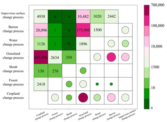
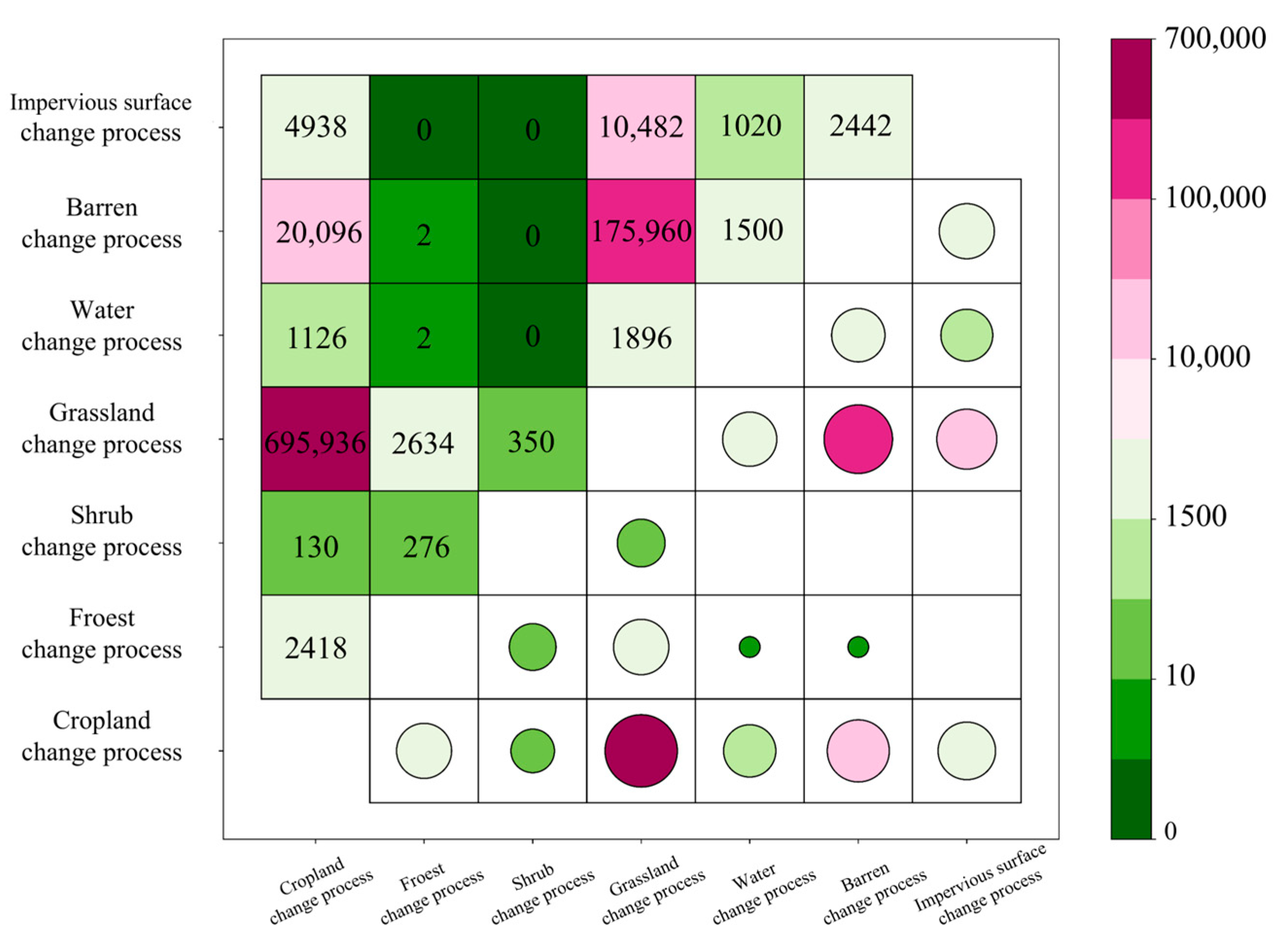
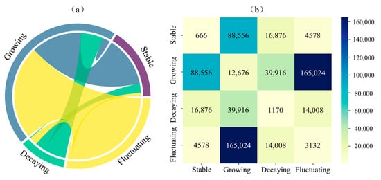
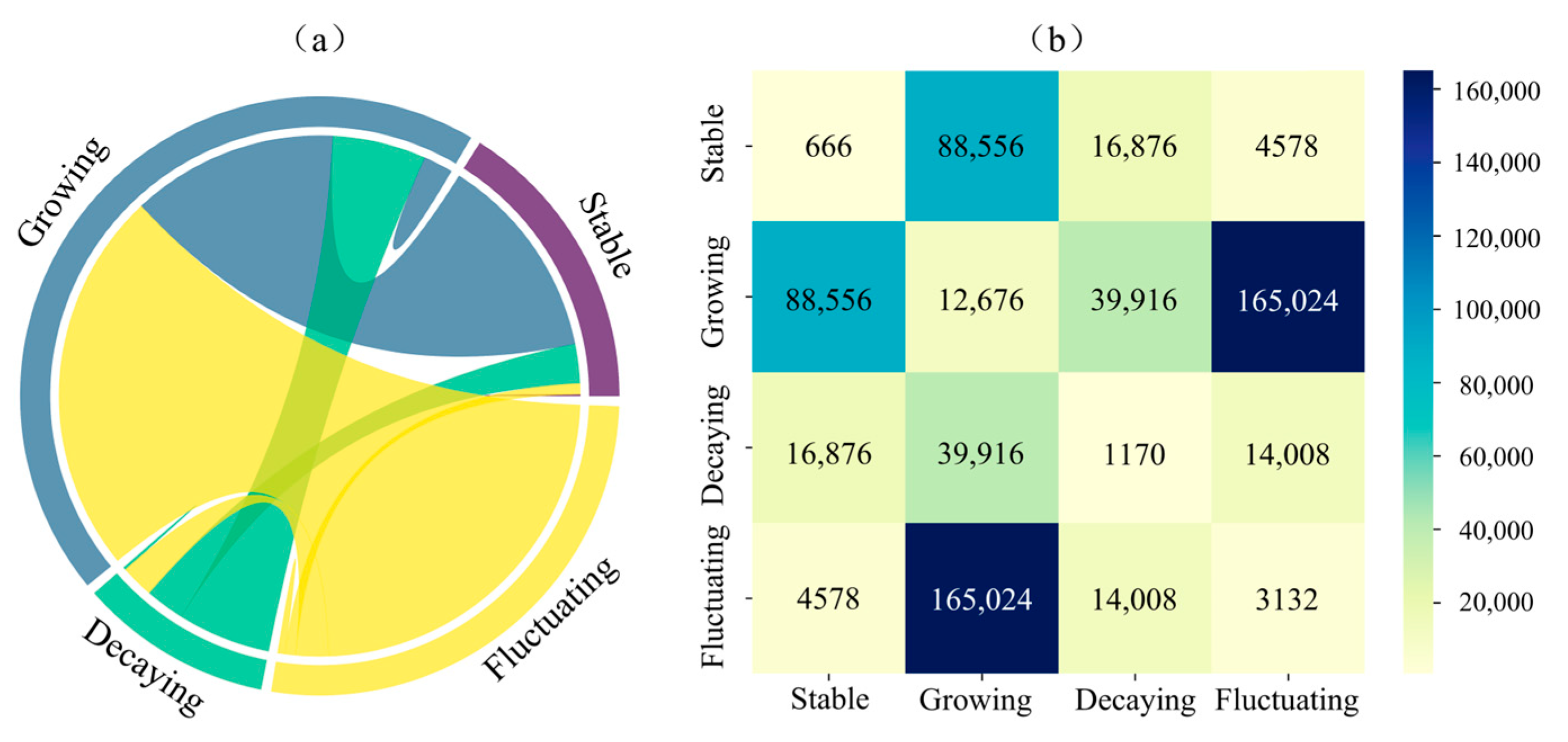
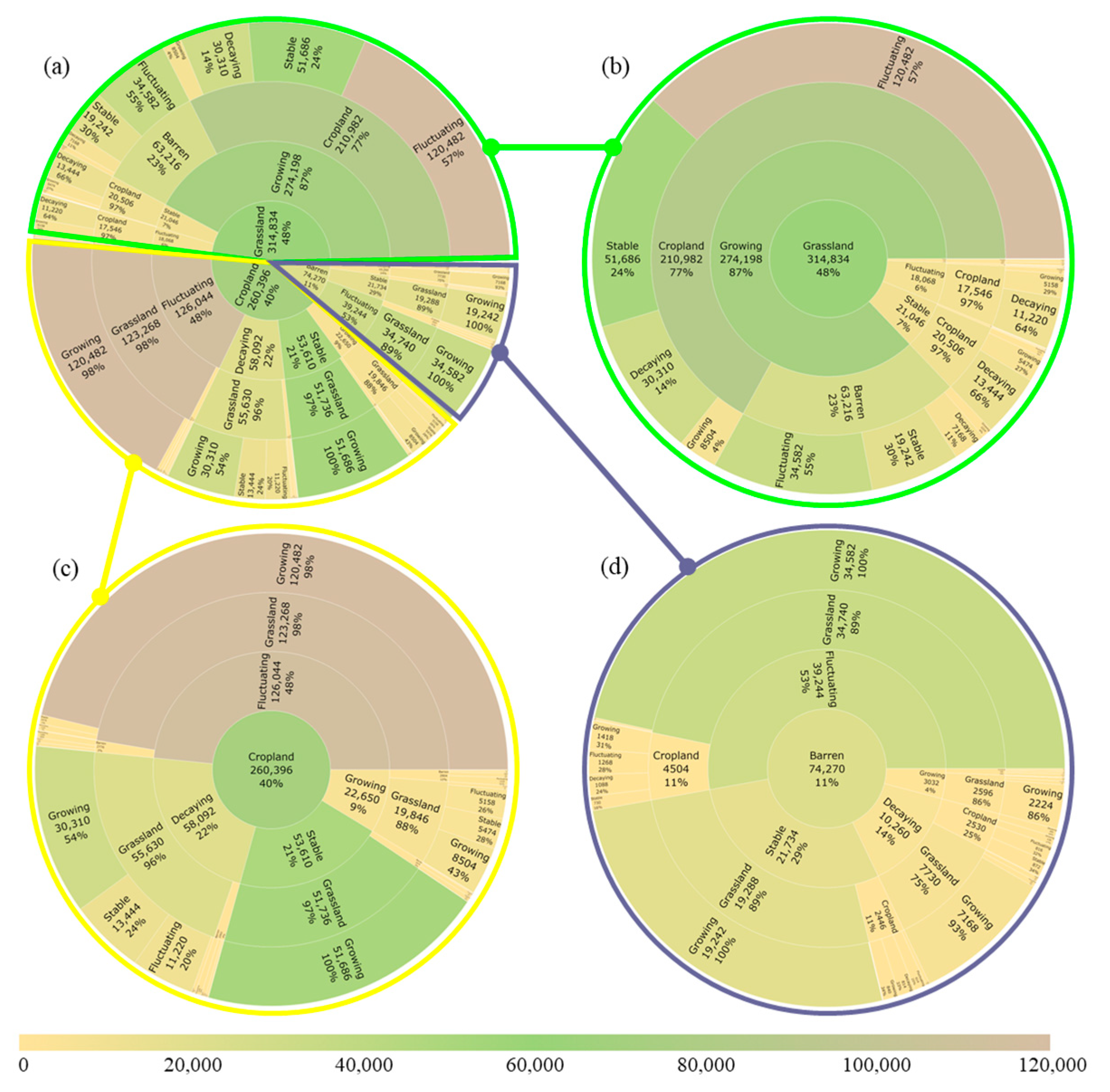
The edge-scale analysis examined interaction mechanisms based on land-cover type, evolutionary state, and composite attributes (Figure 7, Figure 8 and Figure 9).

Figure 7. Edge-scale analysis of land-cover type interaction patterns.

Figure 8. Edge-scale analysis of evolutionary state interaction patterns. (a) Chord diagram of interaction intensity; (b) interaction matrix, where values indicate the number of edges between states.

Figure 9. The interaction patterns between land-cover types and evolutionary states, considered as composite attributes within the NX-LCC-GPO-STG. (a) Multilevel sunburst chart showing the hierarchical distribution of interaction frequencies where integers indicate absolute edge counts and percentages represent the relative share within the parent category; (b–d) detailed connection structures highlighting the primary adjacent combinations for cropland, grassland, and barren change processes, respectively.

Based on the edge-scale analysis of land-cover type interaction patterns (Figure 7), the spatial structure of the study area is primarily shaped by two critical ecological socioeconomic interfaces. First, the dominant high-frequency interactions between cropland change processes and grassland change processes (695,936 edges) indicate that spatial competition and coexistence between agricultural activities and grassland ecosystems constitute the core manifestation of human–environment relationships in the region. Such an extensive contact zone implies extreme sensitivity to drivers like agricultural policy adjustments, climate change, and grazing intensity, making it a focal area for land use conflict and coordination. Second, the interactions between grassland change processes and barren land change processes (175,960 edges) highlight strong ecological tension between vegetation dynamics and desertification processes. This interface embodies ecological vulnerability, indicating that grassland ecosystems are at the forefront of resisting desertification expansion.

The interaction matrix of evolutionary states (Figure 8) reveals a high degree of non-equilibrium, with interactions between growing processes and fluctuating processes dominating the network (165,024 edges). This statistic indicates that active expansion is spatially entangled with high instability, suggesting that growing processes typically occur at the margins of unstable areas or potentially trigger neighboring fluctuations. Conversely, interactions among homogeneous states are extremely rare, as reflected by the low frequency of interactions between stable processes (666 edges) and between decaying processes (1170 edges). This pattern confirms that regional landscape evolution is not defined by synchronous stability or static equilibrium, but is predominantly driven by intense interactions between GPOs exhibiting divergent or opposing evolutionary trajectories.

Figure 9 illustrates the interaction patterns between land-cover types and evolutionary states, considered composite attributes, within the NX-LCC-GPO-STG. This sunburst chart visualizes the hierarchical distribution of edge counts and percentages across four concentric levels including the source land cover, source evolutionary state, target land cover, and target evolutionary state. Specifically, the center and inner rings represent the source attributes while the outer rings detail the target characteristics, with integers denoting absolute edge counts and percentages signifying the relative share within each parent category. These elucidate the spatiotemporal linkages and connectivity relationships among the major land-cover types (grassland, cropland, and barren) and their four evolutionary states (stable, growing, decaying, and fluctuating) within the study area. Statistical results from the global interaction matrix (Figure 9a) and local edge structures (Figure 9b–d) indicate that the combination of the grassland growing process and the cropland fluctuating process ranks first, recording 120,482 edges. This dominant pairing is followed by the interaction between the grassland growing and cropland stable processes (51,686 edges) and the connection between the barren fluctuating and grassland growing processes (34,582 edges).

These interaction patterns reveal a mechanism of land-cover change characterized by high asymmetry and state dependence. The strong reciprocal feedback between grassland growing and cropland fluctuating constitutes the core driving axis of regional dynamics, suggesting that large-scale ecological restoration is intrinsically coupled with agricultural instability, wherein restoration efforts often border or trigger fluctuations in cropland utilization. Furthermore, the significant transitions from barren fluctuating and cropland decaying processes toward grassland growing processes identify grassland as the primary ecological sink and restoration target.

3.4. Subgraph-Scale Analysis for Discovery of Evolution Patterns

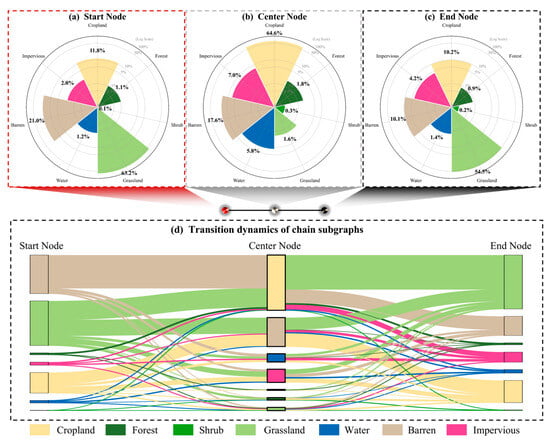
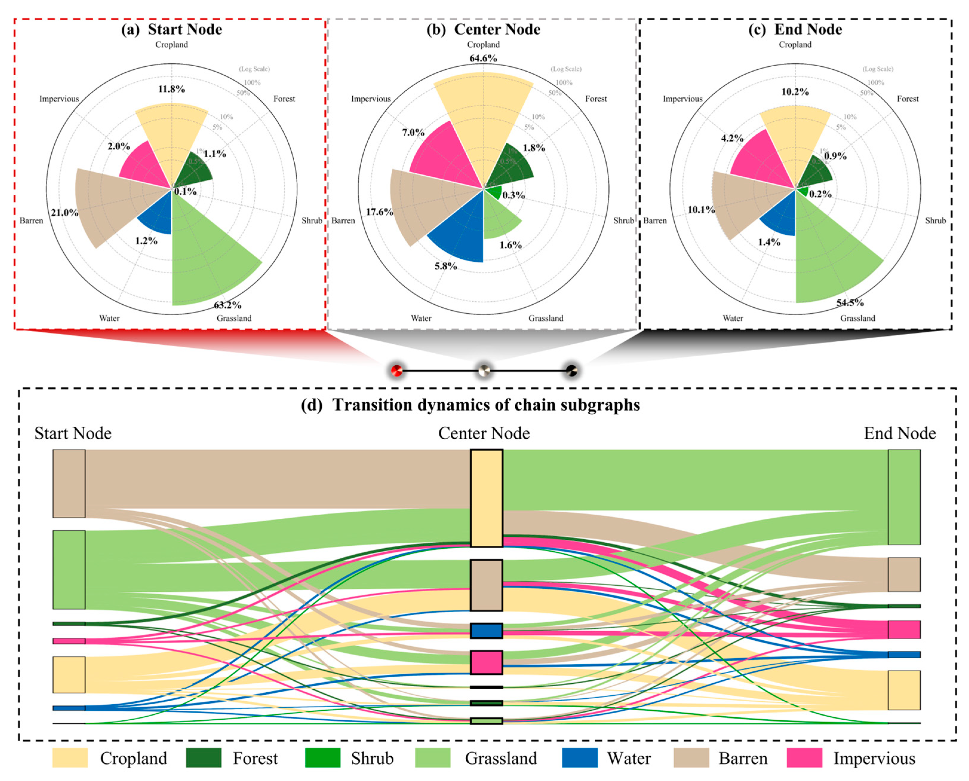
Three-node chain subgraphs were extracted from the NX-LCC-GPO-STG, revealing the sequential evolutionary progression of land-cover change processes across distinct stages. Figure 10 illustrates the substantial shifts in the proportional composition of these change processes observed throughout this evolution.

Figure 10. Proportional composition and transition flows of land-cover change processes across the three-node chain evolution patterns. (a–c) The distribution of land-cover types at the start, center, and end nodes. (d) The transitional flows between these stages.

Examining the proportional composition across the three evolutionary stages, the starting point (Figure 10a) represents relatively natural baseline conditions. Nodes characterized as grassland change processes exert absolute dominance, accounting for 63.21% of the processes, which, combined with barren change processes (20.97%), constitutes the primary foundation of the evolving landscapes. However, the intermediate stage (Figure 10b) marks a dramatic transformation. The proportion of nodes representing grassland change processes collapses to nearly zero (1.61%), replaced by a surge in cropland change processes, which rise sharply to dominance at 64.58%. This indicates that during this phase, the affected areas underwent intense anthropogenic modification, characterized primarily by large-scale agricultural reclamation processes. Significantly, the terminal stage (Figure 10c) reveals that the high-intensity agricultural expansion observed in the intermediate phase was often transient rather than sustained. At this endpoint, the dominance of cropland change processes recedes substantially to 10.17%, coinciding with a marked resurgence of grassland change processes, which reclaim a majority share of 54.48%. The Sankey diagram (Figure 10d) visualizes the transitional flows underpinning these shifts between change processes. The dominant bands illustrate a massive initial conversion from natural starting processes into cropland change processes at the intermediate stage, followed by a significant subsequent flow of cropland reverting back to semi-natural vegetative states (such as grassland change processes) at the terminal stage.

Conclusively, the identified chain patterns reveal a characteristic “utilization–recovery” dynamic trajectory among land-cover change processes. The results demonstrate that significant portions of the study area experienced a transient yet intense peak in agricultural expansion processes (transforming from natural baselines to cropland), followed by a phase of contraction and ecological recovery processes (potentially attributable to cropland abandonment or policy-driven restoration).

4. Discussion

4.1. From State-Based Observation to Process-Oriented Interaction Modeling

The primary contribution of this study is the methodological transition from characterizing “what changed” to understanding “how changes interact”. Conventional approaches often treat landscape evolution as a series of discrete snapshots, which can limit the analysis of causal connectivity between temporal events. The GPO-STG framework builds upon the foundational principles of geographic object-based image analysis (GEOBIA) by extending its spatial logic into the temporal dimension [53,54]. This adaptation involves three specific adjustments to object formation, classification, and topological representation.

Regarding object formation, standard GEOBIA typically derives objects from single-date images based on spatial homogeneity. In this study, GPOs are formed by clustering spatiotemporally contiguous voxels from an annual time series. This approach treats entities as 3D spatiotemporal units rather than 2D spatial patches, allowing for the representation of a process from emergence to disappearance. This modification is intended to address the multi-scale nature of high-resolution imagery where meaningful entities may be better captured across both space and time [53]. Furthermore, the framework adjusts the application of classification and object attributes. Traditional GEOBIA classifies objects based on intrinsic spectral or geometric features to represent the landscape state at a given moment. Building on the use of ontologies to model composite classes [54], the GPO-STG framework incorporates these attributes into graph nodes to facilitate the analysis of STTRs. This transition allows for the quantification of interactions between processes alongside the classification of object states, providing a more integrated view of how different landscape elements influence one another over time. Finally, while traditional GEOBIA often handles temporal analysis through post-classification comparison, our approach integrates spatial and temporal topology within a unified graph structure. By defining edges through quantified relations such as distance, direction, and intensity, the framework models the feedback mechanisms associated with landscape evolution. This integration provides a method to identify coupling patterns, such as the relationship between grassland growing and cropland fluctuating, which may be less apparent when analyzing static snapshots independently. Ultimately, representing the landscape as a network of interacting processes offers a complementary perspective to traditional object-based methods for analyzing land-cover dynamics in dense time series.

4.2. Mechanisms of Landscape Evolution

The application of GPO-STG (NX-LCC-GPO-STG) revealed that landscape evolution is driven by the tension between expansion and instability, rather than synchronous equilibrium. The identification of the dominant interaction between grassland growing processes and cropland fluctuating processes provides quantitative evidence for the utilization–recovery coupling. This pairing suggests that ecological restoration in this region is not an isolated natural recovery, but is intrinsically linked to the instability of agricultural margins. This coupling is likely driven by the synergy between policy-led land conversion and high-frequency climatic variability. Specifically, the implementation of the Grain for Green program enforces a structured replacement of marginal croplands with grasslands, while the inherent precipitation instability in arid zones triggers cyclical feedback where stressed agricultural patches are abandoned and subsequently integrated into the restoration network. Such interactions create a dynamic edge effect where the ecological resilience of grasslands is functionally tethered to the economic vulnerability of croplands. The GPO-STG results demonstrate robust external validity when cross referenced with independent policy records in Ningxia. The framework successfully captured a significant chain of landscape evolution where grassland change processes exert absolute dominance as the natural background before being replaced by a surge in cropland change processes, which finally recede to a minor share of 10.17% as grassland processes reclaim a majority share of 54.48%. This identified sequence aligns precisely with the historical timeline of major regional interventions. The initial agricultural expansion corresponds to the 1978 Shelterbelt Development Program and the requisition compensation balance policy implemented since 1997 to control cultivated land reserves through reclamation [55,56]. The subsequent shift towards ecological restoration matches the 2003 Grazing Ban Policy in Ningxia which forced a reversal of grassland degradation [57]. Furthermore, the marked resurgence of grassland detected between 2011 and 2015 aligns with the large-scale Ecological Migration Project in the Xihaigu region which relocated approximately 350,000 residents and led to widespread farmland abandonment [58]. The capability of the framework to capture these spatiotemporal turning points without prior policy knowledge confirms that this pattern-level validation effectively projects macro-scale socioecological interactions into geographic space. While this study quantifies the strength of these interactions, the specific causal attribution between anthropogenic policy signals and biophysical climate drivers remains a critical frontier for future research.

4.3. Parameter Sensitivity and Optimization in GPO Extraction

The granularity and spatiotemporal integrity of the extracted GPOs are fundamentally governed by the heterogeneity thresholds employed during the segmentation process. These parameters determine the boundary conditions under which local spatiotemporal voxels are aggregated into coherent process objects.

In the context of this study, which utilizes the categorical CLCD, the parameter selection follows a deterministic logic driven by label consistency. Since the semantic definition of a land-cover process relies on the continuity of a single category (e.g., a forest change process must consist strictly of forest pixels). This hard constraint eliminates the ambiguity typically associated with threshold selection, rendering the segmentation results insensitive to parameter fluctuations within the categorical domain. Consequently, the resulting GPOs achieve maximal internal homogeneity, ensuring that the derived evolutionary patterns reflect genuine land-cover transitions rather than artifacts of loose segmentation.

However, the GPO-STG framework is designed to be data-agnostic, and parameter sensitivity becomes a critical consideration when applied to continuous remote sensing data, such as NDVI or surface temperature time series. In such scenarios, the heterogeneity threshold acts as a scale filter: a threshold that is too low may result in the over segmentation of a cohesive process into fragmented patches, whereas a threshold that is too high might merge distinct, albeit similar, processes into a meaningless aggregate. To address this in future applications involving continuous variables, we recommend an adaptive optimization strategy. Statistical methods, such as Otsu’s method or variance-based clustering validation indices, can be employed to dynamically determine the optimal heterogeneity thresholds value. This approach would balance the trade-off between the internal compactness of the GPO and its external separability from the background, thereby ensuring that the extracted processes are physically meaningful and statistically robust.

4.4. Limitations and Future Work

However, this study has limitations that warrant further investigation. The accuracy of GPO extraction is inherently dependent on the quality and temporal consistency of the underlying input data. In this study, we employed the CLCD, which achieves an overall accuracy of 79.31% based on visual interpretation samples and demonstrates superior performance compared to other global land-cover products in independent assessments [46]. However, classification accuracy varies considerably across land-cover types. According to the original validation results, shrubland and grassland exhibit relatively low F1 scores, for instance, 5.30% and 23.98%, respectively, in one validation set, indicating higher uncertainty in these categories. Given that many GPOs are associated with shrub- or grass-dominated ecosystems, such classification uncertainties may propagate into the GPO extraction process, potentially leading to underestimation or omission of certain GPO types. Furthermore, the stability of the generated graph structure is potentially sensitive to the selection of segmentation parameters and the presence of classification noise in the input time series. Although the GPO definition incorporates spatiotemporal constraints to filter out transient pixel-level variations, fluctuations in land-cover labels could still influence the resulting interaction edges. While the current research focuses on establishing the conceptual GPO-STG framework, future work should incorporate systematic parameter sensitivity tests and robustness experiments to further delineate the boundaries of topological stability across diverse landscape conditions. Additionally, while the topological relationships quantify the structure of interactions, they do not explicitly model the physical or socioeconomic drivers (e.g., precipitation anomalies or specific policy enactment dates) behind these edges.

Future work can be advanced by enriching and integrating more attributes. These attributes should encompass diverse environmental and socioeconomic factors. This integration helps clarify the specific driving mechanisms behind the edges. Furthermore, the analysis can be expanded using more graph theory or Graph Neural Network (GNN) methods. These methods effectively mine high-order spatiotemporal patterns within the graph. They significantly enhance the capability to model complex landscape evolution dynamics.

5. Conclusions

The GPO-STG framework was proposed and validated in this study. The analytical unit was shifted from static objects to dynamic GPOs. A unified spatiotemporal edge representation was employed. Consequently, we applied it to the Ningxia Hui Autonomous Region using the CLCD to construct the NX-LCC-GPO-STG, thereby validating the capability of the proposed method.

First, the node-scale analysis revealed that regional landscape dynamics are organized by a small number of high-centrality key processes. Specifically, grassland growing processes act as the key process of the ecosystem, exerting influence on the surrounding landscape organization.

Second, the edge-scale analysis identified a coupling mechanism of restoration and disturbance. The landscape is driven by the intense spatiotemporal interaction between active grassland growing and cropland fluctuating rather than by stable equilibrium.

Third, the subgraph-scale analysis revealed a clear utilization and recovery sequential chain. This finding quantitatively confirms the transition from agricultural expansion to ecological restoration.

Collectively, this study demonstrates the potential of the GPO-STG framework in characterizing the spatiotemporal interactions of RSTS, providing a tool for monitoring land-cover dynamics.

Appendix B.1. Location Feature Extraction

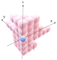
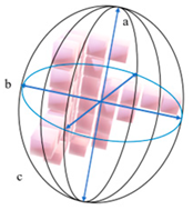
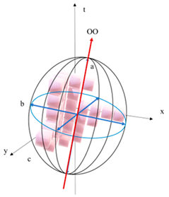
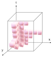
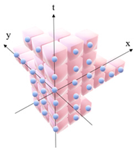
Accurately pinpointing the location of GPOs is vital for effective analysis. This is achieved using various location features, such as the spatiotemporal centroid (STC), overall shape (OS), overall orientation (OO), dimensional range box (DRB), temporal span (TS), and spatial span (SS). Given GPOs are represented by a set of voxel coordinates $[\left(x_1,y_1,t_1\right),\dots ,\left(x_i,y_i,t_i\right),\dots \left(x_m,y_m,t_m\right)]$, with $m$ being the total number of voxels, the details of these metrics are presented in Table A1.

Table A1. Location features of GPOs.

Location Features (Abbreviation)	Equation	Figure	Description
Spatiotemporal Centroid (STC)	$STC=\left({STC}_x,{STC}_y,{STC}_t\right)$ ${STC}_x={\displaystyle \frac{1}{m}}{\displaystyle \sum _{i=1}^m}{x}_i,$ ${STC}_y={\displaystyle \frac{1}{m}}{\displaystyle \sum _{i=1}^m}{y}_i,$ ${STC}_t={\displaystyle \frac{1}{m}}{\displaystyle \sum _{i=1}^m}{t}_i$		Serves as the central reference for spatial analyses of a GPO. It is calculated as the arithmetic mean of voxel coordinates.
Overall Shape (OS)	$OS=(a,b,c)$ $\mathrm{where} a$$\mathrm{is} \mathrm{the} \mathrm{major} \mathrm{principal} \mathrm{axis}. b$$\mathrm{is} \mathrm{the} \mathrm{intermediate} \mathrm{principal} \mathrm{axis}. c$ is the minor principal axis.		Defines a GPO’s spatial configuration using the principal axes of the minimum bounding ellipsoid.
Overall Orientation (OO)	$OO=\mathrm{a}\mathrm{r}\mathrm{c}\mathrm{c}\mathrm{o}\mathrm{s}\left({\displaystyle \frac{a\cdot z}{‖z‖‖z‖}}\right)$ $\mathrm{where} z=\left(\mathrm{0,0},1\right)$$\mathrm{is} \mathrm{the} \mathrm{direction} \mathrm{vector} \mathrm{of} \mathrm{the} \text{t-axis}, ‖a‖$$\mathrm{and} ‖z‖$$\mathrm{represent} \mathrm{the} \mathrm{magnitudes} \mathrm{of} \mathrm{vectors} a$$\mathrm{and} z$.		Determines the angle between the major axis of the minimum bounding ellipsoid and the temporal axis.
Dimensional Range Box (DRB)	$DRB=[x_{min},x_{max},y_{min},$ $y_{max},t_{min},t_{max}]$		Marks the object’s maximum physical boundaries. It defines the smallest three-dimensional envelope containing the GPO.
Temporal Spans (TS)	$TS={t_{max}-t}_{min}$		Indicates the temporal persistence of a GPO. It represents the duration between the earliest and latest points of a GPO’s occurrence.
Spatial Spans (SS)	${SS}_{median}=median\left(A_1,A_2,\dots ,A_n\right),$ ${SS}_{max}=max\left(A_1,A_2,\dots ,A_n\right)$ $\mathrm{where} A_1,A_2,\dots ,A_n$ $\mathrm{are} \mathrm{the} \mathrm{areas} \mathrm{observed} \mathrm{at} \mathrm{different} \mathrm{times} t_1,t_2,\dots ,t_n$.		Quantifies the variations in the spatial footprint of the GPO over time. It is calculated from the median and maximum area projections observed at different time points.

Table A1. Location features of GPOs.

Location Features (Abbreviation)	Equation	Figure	Description
Spatiotemporal Centroid (STC)	$STC=\left({STC}_x,{STC}_y,{STC}_t\right)$ ${STC}_x={\displaystyle \frac{1}{m}}{\displaystyle \sum _{i=1}^m}{x}_i,$ ${STC}_y={\displaystyle \frac{1}{m}}{\displaystyle \sum _{i=1}^m}{y}_i,$ ${STC}_t={\displaystyle \frac{1}{m}}{\displaystyle \sum _{i=1}^m}{t}_i$		Serves as the central reference for spatial analyses of a GPO. It is calculated as the arithmetic mean of voxel coordinates.
Overall Shape (OS)	$OS=(a,b,c)$ $\mathrm{where} a$$\mathrm{is} \mathrm{the} \mathrm{major} \mathrm{principal} \mathrm{axis}. b$$\mathrm{is} \mathrm{the} \mathrm{intermediate} \mathrm{principal} \mathrm{axis}. c$ is the minor principal axis.		Defines a GPO’s spatial configuration using the principal axes of the minimum bounding ellipsoid.
Overall Orientation (OO)	$OO=\mathrm{a}\mathrm{r}\mathrm{c}\mathrm{c}\mathrm{o}\mathrm{s}\left({\displaystyle \frac{a\cdot z}{‖z‖‖z‖}}\right)$ $\mathrm{where} z=\left(\mathrm{0,0},1\right)$$\mathrm{is} \mathrm{the} \mathrm{direction} \mathrm{vector} \mathrm{of} \mathrm{the} \text{t-axis}, ‖a‖$$\mathrm{and} ‖z‖$$\mathrm{represent} \mathrm{the} \mathrm{magnitudes} \mathrm{of} \mathrm{vectors} a$$\mathrm{and} z$.		Determines the angle between the major axis of the minimum bounding ellipsoid and the temporal axis.
Dimensional Range Box (DRB)	$DRB=[x_{min},x_{max},y_{min},$ $y_{max},t_{min},t_{max}]$		Marks the object’s maximum physical boundaries. It defines the smallest three-dimensional envelope containing the GPO.
Temporal Spans (TS)	$TS={t_{max}-t}_{min}$		Indicates the temporal persistence of a GPO. It represents the duration between the earliest and latest points of a GPO’s occurrence.
Spatial Spans (SS)	${SS}_{median}=median\left(A_1,A_2,\dots ,A_n\right),$ ${SS}_{max}=max\left(A_1,A_2,\dots ,A_n\right)$ $\mathrm{where} A_1,A_2,\dots ,A_n$ $\mathrm{are} \mathrm{the} \mathrm{areas} \mathrm{observed} \mathrm{at} \mathrm{different} \mathrm{times} t_1,t_2,\dots ,t_n$.		Quantifies the variations in the spatial footprint of the GPO over time. It is calculated from the median and maximum area projections observed at different time points.

Appendix B.2. Morphological Feature Extraction

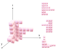
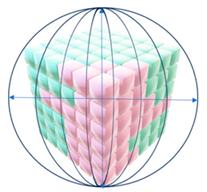
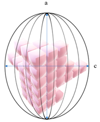
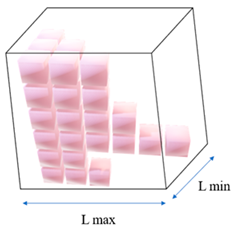
Morphological feature extraction is crucial for delineating the geometric and structural features of GPOs. Morphological features include volume ($Vo$), surface area ($A$), sphericity ($\Psi$), eccentricity ($\epsilon$), and elongation ($L$) (Table A2).

Table A2. Morphological features of GPOs.

Morphological Features (Abbreviation)	Equation	Figure	Description
Volume $(\mathit{V}\mathit{o}$)	$Vo=m\times v_0$ $\mathrm{where} m$$\mathrm{represents} \mathrm{the} \mathrm{number} \mathrm{of} \mathrm{voxels}, \mathrm{and} v_0$ is the volume of each voxel.		Measures the evolutionary duration and extent of a GPO over time, reflecting a GPO’s changes and development in the temporal dimension.
Surface Area $(\mathit{A}$)	$A=6m{a}_0-2s{a}_0$ $\mathrm{where} a_0$$\mathrm{is} \mathrm{the} \mathrm{surface} \mathrm{area} \mathrm{per} \mathrm{face}, \mathrm{and} s$ is the number of adjacent voxels.		Quantifies the geometric complexity of a GPO, where larger surface areas indicate higher complexity and interaction with the surrounding environment.
Sphericity (Ψ)	$\Psi ={\displaystyle \frac{\pi \frac{1}{3}{\left(6Vo\right)}^{\frac{2}{3}}}{A}}$		Quantifies the extent to which a GPO resembles a perfect sphere, with higher values indicating greater sphericity and compactness.
$\mathrm{Eccentricity} (\mathit{\epsilon }$)	$\epsilon =\sqrt{1-{\displaystyle \frac{{\left|c\right|}^2}{{\left|a\right|}^2}}}$		Characterizes the elongation or flatness of a GPO, with higher values indicating a greater departure from a perfect sphere.
Elongation (L)	$L={\displaystyle \frac{L_{max}}{L_{min}}}$		Quantifies the relative length of a GPO in its primary extension direction, with higher values indicating greater elongation.

Table A2. Morphological features of GPOs.

Morphological Features (Abbreviation)	Equation	Figure	Description
Volume $(\mathit{V}\mathit{o}$)	$Vo=m\times v_0$ $\mathrm{where} m$$\mathrm{represents} \mathrm{the} \mathrm{number} \mathrm{of} \mathrm{voxels}, \mathrm{and} v_0$ is the volume of each voxel.		Measures the evolutionary duration and extent of a GPO over time, reflecting a GPO’s changes and development in the temporal dimension.
Surface Area $(\mathit{A}$)	$A=6m{a}_0-2s{a}_0$ $\mathrm{where} a_0$$\mathrm{is} \mathrm{the} \mathrm{surface} \mathrm{area} \mathrm{per} \mathrm{face}, \mathrm{and} s$ is the number of adjacent voxels.		Quantifies the geometric complexity of a GPO, where larger surface areas indicate higher complexity and interaction with the surrounding environment.
Sphericity (Ψ)	$\Psi ={\displaystyle \frac{\pi \frac{1}{3}{\left(6Vo\right)}^{\frac{2}{3}}}{A}}$		Quantifies the extent to which a GPO resembles a perfect sphere, with higher values indicating greater sphericity and compactness.
$\mathrm{Eccentricity} (\mathit{\epsilon }$)	$\epsilon =\sqrt{1-{\displaystyle \frac{{\left|c\right|}^2}{{\left|a\right|}^2}}}$		Characterizes the elongation or flatness of a GPO, with higher values indicating a greater departure from a perfect sphere.
Elongation (L)	$L={\displaystyle \frac{L_{max}}{L_{min}}}$		Quantifies the relative length of a GPO in its primary extension direction, with higher values indicating greater elongation.

Appendix B.3. Evolutionary Feature Extraction

Evolutionary features capture how GPOs change over time, thereby clarifying their dynamic nature. This requires explicitly representing the inherent temporal information in GPOs to elucidate their evolutionary patterns.

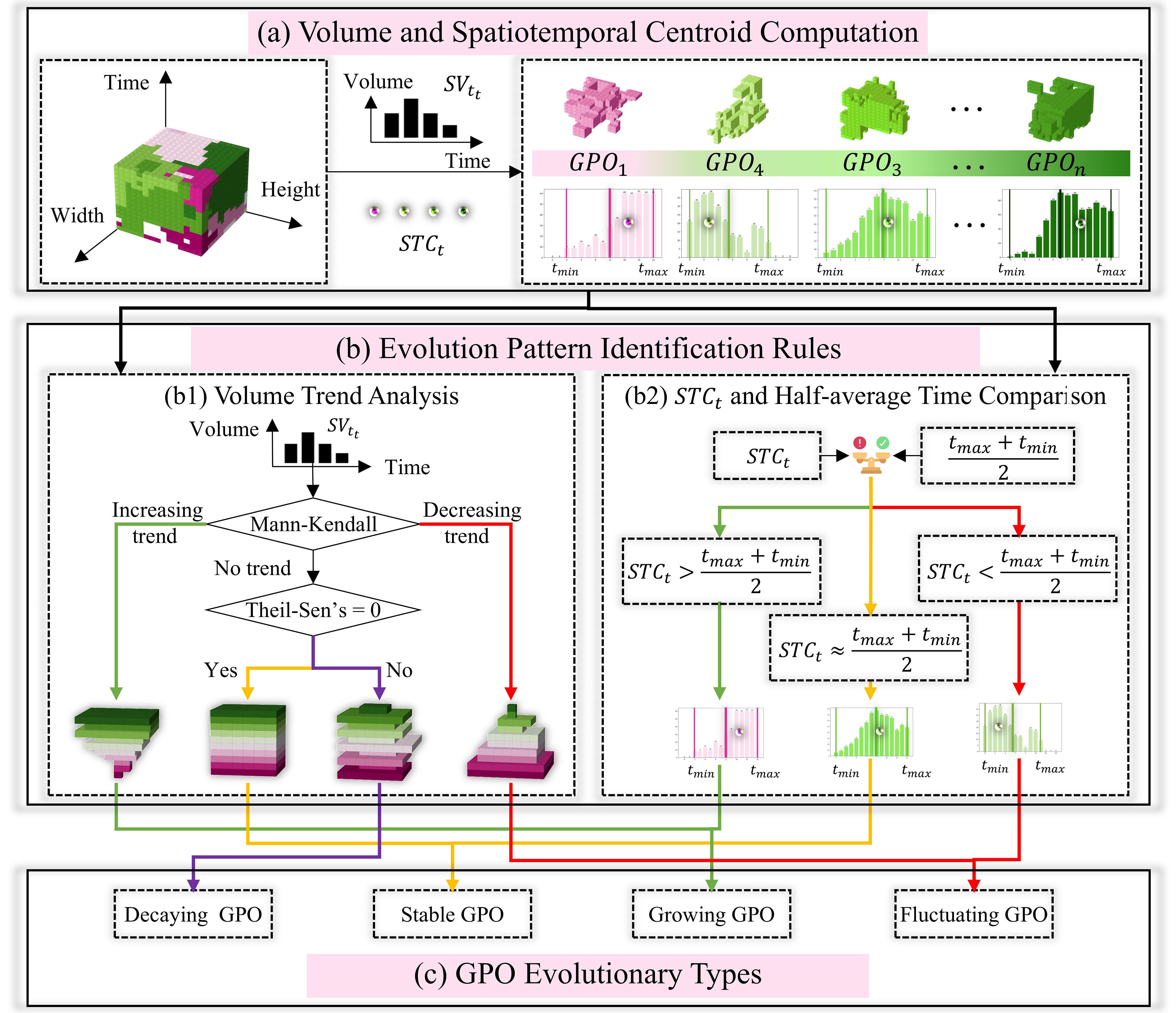
Figure A1 shows a rule-based method for identifying the evolution dynamics of GPOs. This method comprises three main steps. The first step involves computing the volume (${SV}_{t_t}$) and the time component of STC (${STC}_t$) for each GPO (Figure A1a). ${SV}_{t_t}$ represents the total volume of the object at time step ${\mathrm{t}}_{\mathrm{t}}$, and ${STC}_t$ denotes the average location of the object (Table A1). The second step involves identifying the GPO’s evolution patterns (Figure A1b). This involves two main analyses. First, volume trend analysis (Figure A1(b1)) is performed using the Mann–Kendall trend test to assess the trend of the GPO volume over time. A statistically significant positive (negative) trend from the Mann–Kendall test indicates that the object is growing (decaying). If no statistically significant trend is detected, then the Theil–Sen slope is evaluated. A zero (nonzero) slope implies that the object is stable (fluctuating). Second, ${STC}_t$ is compared with the half-average time (Figure A1(b2)), which represents the median time step of the object’s existence. If ${STC}_t$ is larger (smaller) than the half-average time, then the object is growing (decaying). An ${STC}_t$ close to the half-average time indicates that the object is stable. The final step (Figure A1c), which combines volume trend analysis and ${STC}_t$ comparison to determine the evolution type, integrates the information obtained from both analyses to ascertain the overall GPO evolution type. An object is considered stable if the volume trend is insignificant and ${STC}_t$ is close to the half-average time; it is considered growing if the volume trend is positive and ${STC}_t$ is larger than the half-average time. It is deemed decaying if the volume trend is negative and the ${STC}_t$ is smaller than the half-average time; if the volume trend is not consistently positive or negative and ${STC}_t$ does not exhibit a clear pattern relative to the half-average time, then the object is classified as fluctuating.

Figure A1. Rule-based identification of GPO evolution types: (a) Computation of volume (${SV}_{t_t}$) and time component of STC (${STC}_t$) for each GPO, (b) GPO evolution pattern recognition rules, subdivided into (b1) volume trend analysis (using Mann–Kendall trend test and Theil–Sen slope estimation) and (b2) comparison of ${STC}_t$ and half-average time, and (c) determination of four GPO evolution types (decaying, stable, growing, and fluctuating).

Figure A1. Rule-based identification of GPO evolution types: (a) Computation of volume (${SV}_{t_t}$) and time component of STC (${STC}_t$) for each GPO, (b) GPO evolution pattern recognition rules, subdivided into (b1) volume trend analysis (using Mann–Kendall trend test and Theil–Sen slope estimation) and (b2) comparison of ${STC}_t$ and half-average time, and (c) determination of four GPO evolution types (decaying, stable, growing, and fluctuating).

References

- Pettorelli, N.; Vik, J.O.; Mysterud, A.; Gaillard, J.-M.; Tucker, C.J.; Stenseth, N.C. Using the satellite-derived NDVI to assess ecological responses to environmental change. Trends Ecol. Evol. 2005, 20, 503–510. [Google Scholar] [CrossRef] [Scilit] [PubMed]
- Berra, E.F.; Fontana, D.C.; Yin, F.; Breunig, F.M. Harmonized Landsat and Sentinel-2 Data with Google Earth Engine. Remote Sens. 2024, 16, 2695. [Google Scholar] [CrossRef] [Scilit]
- Wulder, M.A.; Coops, N.C. Satellites: Make Earth observations open access. Nature 2014, 513, 30–31. [Google Scholar] [CrossRef] [Scilit] [PubMed]
- Zhu, Z.; Woodcock, C.E. Continuous change detection and classification of land cover using all available Landsat data. Remote Sens. Environ. 2014, 144, 152–171. [Google Scholar] [CrossRef] [Scilit]
- Chen, L.; Sun, R.; Lu, Y. A conceptual model for a process-oriented landscape pattern analysis. Sci. China Earth Sci. 2019, 62, 2050–2057. [Google Scholar] [CrossRef] [Scilit]
- Verbesselt, J.; Hyndman, R.; Newnham, G.; Culvenor, D. Detecting trend and seasonal changes in satellite image time series. Remote Sens. Environ. 2010, 114, 106–115. [Google Scholar] [CrossRef] [Scilit]
- Xue, C.; Su, F.; He, Y. Process: A New View of Geographical Spatiotemporal Dynamic Analysis. Adv. Earth Sci. 2022, 37, 65–79. [Google Scholar] [CrossRef]
- Verbesselt, J.; Hyndman, R.; Zeileis, A.; Culvenor, D. Phenological change detection while accounting for abrupt and gradual trends in satellite image time series. Remote Sens. Environ. 2010, 114, 2970–2980. [Google Scholar] [CrossRef] [Scilit]
- Kennedy, R.E.; Yang, Z.; Cohen, W.B. Detecting trends in forest disturbance and recovery using yearly Landsat time series: 1. LandTrendr—Temporal segmentation algorithms. Remote Sens. Environ. 2010, 114, 2897–2910. [Google Scholar] [CrossRef] [Scilit]
- Ye, S.; Zhu, Z.; Cao, G. Object-based continuous monitoring of land disturbances from dense Landsat time series. Remote Sens. Environ. 2023, 287, 113462. [Google Scholar] [CrossRef] [Scilit]
- Huang, C.; Goward, S.N.; Masek, J.G.; Thomas, N.; Zhu, Z.; Vogelmann, J.E. An automated approach for reconstructing recent forest disturbance history using dense Landsat time series stacks. Remote Sens. Environ. 2010, 114, 183–198. [Google Scholar] [CrossRef] [Scilit]
- Yan, Z.; Ma, L.; He, W.; Zhou, L.; Lu, H.; Liu, G.; Huang, G. Comparing Object-Based and Pixel-Based Methods for Local Climate Zones Mapping with Multi-Source Data. Remote Sens. 2022, 14, 3744. [Google Scholar] [CrossRef] [Scilit]
- Bhatt, A.; Ghosh, S.K.; Kumar, A. Spectral indices based object oriented classification for change detection using satellite data. Int. J. Syst. Assur. Eng. Manag. 2018, 9, 33–42. [Google Scholar] [CrossRef] [Scilit]
- Huang, F.; Chen, L.; Yin, K.; Huang, J.; Gui, L. Object-oriented change detection and damage assessment using high-resolution remote sensing images, Tangjiao Landslide, Three Gorges Reservoir, China. Environ. Earth Sci. 2018, 77, 183. [Google Scholar] [CrossRef] [Scilit]
- Wu, L.; Liu, X.; Liu, M.; Yang, J.; Zhu, L.; Zhou, B. Online Forest Disturbance Detection at the Sub-Annual Scale Using Spatial Context From Sparse Landsat Time Series. IEEE Trans. Geosci. Remote Sens. 2022, 60, 1–14. [Google Scholar] [CrossRef] [Scilit]
- Rajbhandari, S. Methodological Framework for Ontology-Driven Geographic Object-Based Image Analysis (O-GEOBIA). Ph.D. Thesis, University of Tasmania, Sandy Bay, Australia, 2019. [Google Scholar]
- Rajbhandari, S.; Aryal, J.; Osborn, J.; Lucieer, A.; Musk, R. Leveraging Machine Learning to Extend Ontology-Driven Geographic Object-Based Image Analysis (O-GEOBIA): A Case Study in Forest-Type Mapping. Remote Sens. 2019, 11, 503. [Google Scholar] [CrossRef] [Scilit]
- Şener, Z.; Uzar, M.; Musaoglu, N.; Basaraner, M. Using Ontology in Object Based Image Classification. In Proceedings of the International Symposium on Applied Geoinformatics (ISAG-2019), Istanbul, Turkey, 7–9 November 2019. [Google Scholar]
- Yuan, F.; Zhang, P.; Zhang, Q.; Zhang, Y.; Wang, A. Representing the Spatiotemporal State Evolution of Geographic Entities as a Multi-Level Graph. Remote Sens. 2025, 14, 252. [Google Scholar] [CrossRef] [Scilit]
- Oliva Santos, R.; Maciá Pérez, F.; Garea Llano, E. Ontology-based topological representation of remote-sensing images. ISPRS Int. J. Geo-Inf. 2014, 35, 16–28. [Google Scholar] [CrossRef] [Scilit]
- Sui, H.; Feng, W.; Li, W.; Sun, K.; Xu, C. Review of Change Detection Methods for Multi-temporal Remote Sensing Imagery. Geomat. Inf. Sci. Wuhan Univ. 2018, 43, 1885–1898. [Google Scholar] [CrossRef]
- Zhang, L.; Wang, S.; Zhu, M.; Liu, H.; Gao, L.; Lin, Y.; Wang, J.; Tong, Q. From Spectrum to Spectrotemporal: Research on Time Series Change Detection of Remote Sensing. Geomat. Inf. Sci. Wuhan Univ. 2021, 46, 451–468. [Google Scholar] [CrossRef]
- Cheung, A.K.L.; Brierley, G.; O’Sullivan, D. Landscape structure and dynamics on the Qinghai-Tibetan Plateau. Ecol. Model. 2016, 339, 7–22. [Google Scholar] [CrossRef] [Scilit]
- Hong, D.; Gao, L.; Yao, J.; Zhang, B.; Plaza, A.; Chanussot, J. Graph Convolutional Networks for Hyperspectral Image Classification. IEEE Trans. Geosci. Remote Sens. 2021, 59, 5966–5978. [Google Scholar] [CrossRef] [Scilit]
- Dufourg, C.; Pelletier, C.; May, S.; Lefèvre, S. On the Use of Graphs for Satellite Image Time Series: A comprehensive review. IEEE Geosci. Remote Sens. Mag. 2025, 14, 205–244. [Google Scholar] [CrossRef] [Scilit]
- Cheung, A.K.L.; O’Sullivan, D.; Brierley, G. Graph-assisted landscape monitoring. Int. J. Geogr. Inf. Sci. 2015, 29, 580–605. [Google Scholar] [CrossRef] [Scilit]
- Guttler, F.; Ienco, D.; Nin, J.; Teisseire, M.; Poncelet, P. A graph-based approach to detect spatiotemporal dynamics in satellite image time series. ISPRS J. Photogramm. Remote Sens. 2017, 130, 92–107. [Google Scholar] [CrossRef] [Scilit]
- Khiali, L.; Ienco, D.; Teisseire, M. Object-oriented satellite image time series analysis using a graph-based representation. Ecol. Inform. 2018, 43, 52–64. [Google Scholar] [CrossRef] [Scilit]
- Khiali, L.; Ndiath, M.; Alleaume, S.; Ienco, D.; Ose, K.; Teisseire, M. Detection of spatio-temporal evolutions on multi-annual satellite image time series: A clustering based approach. Int. J. Appl. Earth Obs. Geoinf. 2019, 74, 103–119. [Google Scholar] [CrossRef] [Scilit]
- Wu, B.; Yu, B.; Shu, S.; Wu, Q.; Zhao, Y.; Wu, J. A spatiotemporal structural graph for characterizing land cover changes. Int. J. Geogr. Inf. Sci. 2021, 35, 397–425. [Google Scholar] [CrossRef] [Scilit]
- Zou, X.; Liu, X.; Liu, M.; Tian, L.; Zhu, L.; Zhang, Q. Spatiotemporal graph-based analysis of land cover evolution using remote sensing time series data. Int. J. Geogr. Inf. Sci. 2023, 37, 1009–1040. [Google Scholar] [CrossRef] [Scilit]
- Wen, Y.; Liu, M.; Wu, Z.; Zhang, Q.; Su, J.; Hu, Z. Spatiotemporal graph for detecting evolution characteristics of karst rocky desertification from long time-series Landsat images. Catena 2026, 262, 109697. [Google Scholar] [CrossRef] [Scilit]
- Liu, M.; Liu, X.; Wu, L.; Peng, T.; Zhang, Q.; Zou, X.; Tian, L.; Wang, X. Hybrid Spatiotemporal Graph Convolutional Network for Detecting Landscape Pattern Evolution From Long-Term Remote Sensing Images. IEEE Trans. Geosci. Remote Sens. 2022, 60, 1–16. [Google Scholar] [CrossRef] [Scilit]
- Tian, L.; Liu, X.; Liu, M.; Wu, L. State-and-Evolution Detection Models: A Framework for Continuously Monitoring Landscape Pattern Change. IEEE Trans. Geosci. Remote Sens. 2021, 60, 1–14. [Google Scholar] [CrossRef] [Scilit]
- Tian, L.; Meng, Y.; Zhu, L.; Zou, X.; Liu, X. Graph-based spatial pattern multi-type change detection. ISPRS J. Photogramm. Remote Sens. 2023, 199, 258–271. [Google Scholar] [CrossRef] [Scilit]
- Li, L.; Xu, Y.; Xue, C.; Fu, Y.; Zhang, Y. A Process-Oriented Approach to Identify Evolutions of Sea Surface Temperature Anomalies with a Time-Series of a Raster Dataset. ISPRS Int. J. Geo-Inf. 2021, 10, 500. [Google Scholar] [CrossRef] [Scilit]
- Peuquet, D.J. Making space for time: Issues in space-time data representation. GeoInformatica 2001, 5, 11–32. [Google Scholar] [CrossRef] [Scilit]
- Xi, W.; Du, S.; Wang, Y.-C.; Zhang, X. A spatiotemporal cube model for analyzing satellite image time series: Application to land-cover mapping and change detection. Remote Sens. Environ. 2019, 231, 111212. [Google Scholar] [CrossRef] [Scilit]
- Bach, B.; Dragicevic, P.; Archambault, D.; Hurter, C.; Carpendale, S. A Descriptive Framework for Temporal Data Visualizations Based on Generalized Space-Time Cubes. Comput. Graph. Forum 2017, 36, 36–61. [Google Scholar] [CrossRef] [Scilit]
- Zhang, H.; Zhou, X.; Yang, Y.; Wang, H.; Ye, X.; Tang, G. Advancing Process-Oriented Geographical Regionalization Model. Ann. Am. Assoc. Geogr. 2024, 114, 2388–2413. [Google Scholar] [CrossRef] [Scilit]
- Wang, N.; Li, W.; Tao, R.; Du, Q. Graph-based block-level urban change detection using Sentinel-2 time series. Remote Sens. Environ. 2022, 274, 112993. [Google Scholar] [CrossRef] [Scilit]
- Roy, A.; Roy, K.K.; Ali, A.A.; Amin, M.A.; Rahman, A.K.M.M. Unified Spatio-Temporal Modeling for Traffic Forecasting using Graph Neural Network. In Proceedings of the 2021 International Joint Conference on Neural Networks (IJCNN), Shenzhen, China, 18–22 July 2021; pp. 1–8. [Google Scholar]
- Luo, J.; Wu, T.; Wu, Z.; Zhou, Y.; Gao, L.; Sun, Y.; Wu, W.; Yang, Y.; Hu, X.; Zhang, X.; et al. Methods of Intelligent Computation and Pattern Mining based on Geo-parcels. J. Geo-Inf. Sci. 2020, 22, 57–75. [Google Scholar] [CrossRef]
- Zhou, X.; Zhang, H.; Ye, X. A multi-hierarchical method to extract spatial network structures from large-scale origin-destination flow data. Int. J. Geogr. Inf. Sci. 2024, 38, 577–602. [Google Scholar] [CrossRef] [Scilit]
- Domenico, M.D. More is different in real-world multilayer networks. Nat. Phys. 2023, 19, 1247–1262. [Google Scholar] [CrossRef] [Scilit]
- Yang, J.; Huang, X. The 30 m annual land cover dataset and its dynamics in China from 1990 to 2019. Earth Syst. Sci. Data 2021, 13, 3907–3925. [Google Scholar] [CrossRef] [Scilit]
- Belussi, A.; Migliorini, S.; Negri, M. A framework for evaluating 3D topological relations based on a vector data model. GeoInformatica 2020, 24, 915–950. [Google Scholar] [CrossRef] [Scilit]
- Sisi, Z. Topological Relationships and Their Use. 2015. Available online: https://onlinelibrary.wiley.com/doi/epdf/10.1111/j.1461-0248.2008.01271.x (accessed on 1 January 2024).
- Zanin, M.; Belkoura, S.; Gomez, J.; Alfaro, C.; Cano, J. Topological structures are consistently overestimated in functional complex networks. Sci. Rep. 2018, 8, 11980. [Google Scholar] [CrossRef] [Scilit]
- Leopold, J.L.; Sabharwal, C.L.; Ward, K.J. Spatial relations between 3D objects: The association between natural language, topology, and metrics. J. Vis. Lang. Comput. 2015, 27, 29–37. [Google Scholar] [CrossRef] [Scilit]
- Allen, J.F. Maintaining Knowledge about Temporal Intervals. In Readings in Qualitative Reasoning About Physical Systems; Morgan Kaufmann: San Francisco, CA, USA, 1990; Volume 26, pp. 361–372. [Google Scholar]
- Egenhofer, M.J.; Herring, J.R. Categorizing binary topological relations between regions, lines and points in geographic databases. Stat. Inf. Forum 1990, 9, 76. [Google Scholar]
- Blaschke, T. Object based image analysis for remote sensing. ISPRS J. Photogramm. Remote Sens. 2010, 65, 2–16. [Google Scholar] [CrossRef] [Scilit]
- Blaschke, T.; Hay, G.J.; Kelly, M.; Lang, S.; Hofmann, P.; Addink, E.; Queiroz Feitosa, R.; van der Meer, F.; van der Werff, H.; van Coillie, F.; et al. Geographic Object-Based Image Analysis—Towards a new paradigm. ISPRS J. Photogramm. Remote Sens. 2014, 87, 180–191. [Google Scholar] [CrossRef] [Scilit]
- Li, W.; Wang, D.; Liu, S.; Zhu, Y.; Yan, Z. Reclamation of Cultivated Land Reserves in Northeast China: Indigenous Ecological Insecurity Underlying National Food Security. Int. J. Environ. Res. Public Health 2020, 17, 1211. [Google Scholar] [CrossRef] [Scilit] [PubMed]
- Mitchell, D.J.; Fullen, M.A.; Trueman, I.C.; Fearnehough, W. Sustainability of reclaimed desertified land in Ningxia, China. J. Arid. Environ. 1998, 39, 239–251. [Google Scholar] [CrossRef] [Scilit]
- Chen, Y.; Zhou, L. Farmers’ Perception of the Decade-Long Grazing Ban Policy in Northern China: A Case Study of Yanchi County. Sustainability 2016, 8, 1113. [Google Scholar] [CrossRef] [Scilit]
- Zheng, Y.; Meng, H.; Xie, X.; Shi, S. Dynamics of Climate Change, Drought and Migration: A Mixed Method Research in Ningxia. Chn. J. Urb. Environ.Stud. 2017, 5, 1750021. [Google Scholar] [CrossRef] [Scilit]
- Zhang, Y.; Liu, X.; Liu, M.; Zou, X.; Zhang, Q.; Peng, T. Multi-Scale Spatiotemporal Change Characteristics Analysis of High-Frequency Disturbance Forest Ecosystem Based on Improved Spatiotemporal Cube Model. Remote Sens. 2021, 13, 2537. [Google Scholar] [CrossRef] [Scilit]
- Gray, J.; Chaudhuri, S.; Bosworth, A.; Layman, A.; Reichart, D.; Venkatrao, M.; Pellow, F.; Pirahesh, H. Data cube: A relational aggregation operator generalizing group-by, cross-tab, and sub-totals. Data Min. Knowl. Discov. 1997, 1, 29–53. [Google Scholar] [CrossRef] [Scilit]
- Wang, Y.; Zhang, F. An Unified CGA-Based Formal Expression of Spatio-Temporal Topological Relations for Computation and Analysis of Geographic Objects. Adv. Appl. Clifford Algebr. 2019, 29, 59. [Google Scholar] [CrossRef] [Scilit]
Disclaimer/Publisher’s Note: The statements, opinions and data contained in all publications are solely those of the individual author(s) and contributor(s) and not of MDPI and/or the editor(s). MDPI and/or the editor(s) disclaim responsibility for any injury to people or property resulting from any ideas, methods, instructions or products referred to in the content. |
© 2026 by the authors. Licensee MDPI, Basel, Switzerland. This article is an open access article distributed under the terms and conditions of the Creative Commons Attribution (CC BY) license.